Diagnosing failures of fairness transfer across distribution shift in real-world medical settings

Abstract

Diagnosing and mitigating changes in model fairness under distribution shift is an important component of the safe deployment of machine learning in healthcare settings. Importantly, the success of any mitigation strategy strongly depends on the structure of the shift. Despite this, there has been little discussion of how to empirically assess the structure of a distribution shift that one is encountering in practice. In this work, we adopt a causal framing to motivate conditional independence tests as a key tool for characterizing distribution shifts. Using our approach in two medical applications, we show that this knowledge can help diagnose failures of fairness transfer, including cases where real-world shifts are more complex than is often assumed in the literature. Based on these results, we discuss potential remedies at each step of the machine learning pipeline.

1 Introduction

As progress is made to integrate machine learning (ML) systems in real-world applications, one concern is how the ML model’s behaviour might be affected by changes in the data distribution. While extensive work has investigated the effect of distribution shift on ML model performance [see 50, 80, 22, 77, for reviews], recent work has also highlighted that fairness properties that are satisfied on the data used to develop a model might not always hold if the data distribution changes [36, 32]. In high-risk domains like healthcare, this can translate to ‘if a model satisfies fairness criteria when trained in “Hospital A”, it may not satisfy them when tested in “Hospital B”’. Fueled by this observation, a new field of research is emerging to understand the relationship between ML fairness and robustness to distribution shift [e.g. 64, 1, 75, 16, 88, 68] and to provide mitigation techniques for obtaining robustly fair ML models [e.g. 67, 70, 69, 89, 15].

Importantly, the success of robustly fair machine learning depends strongly on the nature of the distribution shifts that the system will encounter in practice. This point has been made elegantly in existing work as a motivation to use causal structure to provide fairness guarantees for specified distribution shifts [67, 70]. However, to the best of our knowledge, few methods can diagnose the nature of the shift and guide towards an appropriate mitigation strategy [69].

In this work, we design statistical tests that can, based on a simplified causal graph of an application and a small target dataset, assess the structure of the distribution shift encountered by the system and identify aspects of the data that hinder the transfer of fairness properties. Using applications in dermatology and Electronic Health Records (EHR), we show that this analysis is crucial for selecting an appropriate mitigation strategy. Further, our work also reveals that clinically plausible shifts are often more complex than can be handled by current mitigation techniques, highlighting the need for additional research into a broader set of remedies across the entire ML pipeline.

2 Background

Notation

We consider problems where we are given variables $X$, $A$, $Y$, where $X$ is a set of features, $A$ is one or more sensitive attributes, and $Y$ is an outcome or label to be predicted. Our goal is to build a classification or regression model $f(X^{\prime})$, where, depending on the context, $X^{\prime}:=(X,A)$ or $X^{\prime}:=X$. We are concerned with the fairness properties of $f$, both on the training distribution and in one or more deployed environments. Depending on the setting, we focus on several statistical definitions of fairness [5]: gaps in subgroup accuracy, demographic parity, and equalized odds. See the Supplement for their formulation.

Formally, we represent distribution shifts using the so-called Joint Causal Inference (JCI) framework of Mooij et al. [45]. We represent causal relationships between elements of $A$, $X$, $Y$ in a causal Bayesian network (CBN, see the Supplement for an introduction). In a CBN, a node $U^{i}$ with an arrow into $U^{j}$ is called a direct cause of $U^{j}$. We call all direct causes of a node $U^{i}$ its causal parents, and denote them ${\text{pa}}(U^{i})$. To represent shifts, we augment the CBN with an environment variable $S$, where the event $S=0$ indicates data from the source environment and $S=1$ denotes data from the target environment, so that source data are distributed according to $P(A,X,Y\mid S=0)$ and the target data to $P(A,X,Y\mid S=1)$. This is called the joint causal graph. In the joint causal graph, arrows from $S$ denote changes to statistical relationships that are induced by the shift. Specifically, an arrow from $S$ to some variable $U$ indicates that the conditional distribution of that variable given its causal parents could change between training and deployment environments, while the absence of such an arrow would indicate that the conditional distribution remains the same, i.e. $P(U\mid{\text{pa}}(U),S=0)=P(U\mid{\text{pa}}(U),S=1)$.

Components of Distribution Shifts

In JCI formalism, the components of a distribution shift are represented by direct arrows from the shift variable $S$ to variables $A$, $Y$, and $X$. Here, we briefly summarize how these arrows can be interpreted. $S\rightarrow A$ arrows represent demographic shifts, implying $P(A\mid S=s)$ changes for different values of $s$. An example of such a shift is a difference in the age distribution of patients in $S=0$ versus $S=1$. $S\rightarrow X$ arrows represent covariate shifts, where the conditional distribution of input features $P(X\mid{\text{pa}}(X),S=s)$ changes for different values of $s$. For example such a shift could result form using different cameras or views to acquire an image in $S=0$ and $S=1$ (c.f., acquisition shift in Castro and Glocker [7]). Finally, $S\rightarrow Y$ arrows represent label shifts, where the conditional distribution of labels $P(Y\mid{\text{pa}}(Y),S=s)$ changes for different values of $s$. A label shift can occur through different disease prevalences, or different strategies for obtaining labels, across $S=0$ and $S=1$ (c.f., prevalence shift and annotation shift, respectively, in Castro and Glocker [7]).

In real-world applications, distribution shifts often include multiple components, where there are multiple arrows from $S$ to $\{A,X,Y\}$. We call such shifts compound. Compound shifts often occur when there is an unobserved variable that affects multiple variables whose distribution changes between source and target. An example is that of a new device on the market [24]. Such a device could create qualitatively different images $X$, but it could also change the observed patient population by being made more available to certain subsets of demographic groups that tend to be more or less healthy. In this case, the shift induced by introducing the device simultaneously affects $A,X$ and $Y$.

Shift Structure and Fairness Transfer

The transfer of fairness depends on the causal structure of the application and the structure of the shift [67, 68]. In particular, implications for fairness transfer can be directly read off of conditional independences with respect to the shift $S$ in the joint causal graph. For example, for classifiers that take a set of variables $\{\mathbf{V}\}$ as input, the following metrics are known to be invariant across the shift under the following conditional independence conditions:

• Classification error ($P(Y\neq f(\mathbf{V})\mid\mathbf{V},S)$) is invariant if $Y\mathrel{\perp\mspace{-10.0mu}\perp}S\,|\,\{\mathbf{V}\}$ [41, 67].

• Demographic parity gap ($\max_{a\in\mathcal{A}}E[f(\mathbf{V})\mid S,A=a]-\min_{a\in\mathcal{A}}E[f(\mathbf{V})\mid S,A=a]$) is invariant if $\{\mathbf{V}\}\mathrel{\perp\mspace{-10.0mu}\perp}S\,|\,A$ [67].

• Equality of odds gap ($\max_{a,y\in\mathcal{A}x\mathcal{Y}}E[f(\mathbf{V})\mid S,A=a,Y=y]-\min_{a,y\in\mathcal{A}x\mathcal{Y}}E[f(\mathbf{V})\mid S,A=a,Y=y]$) is invariant if $\{\mathbf{V}\}\mathrel{\perp\mspace{-10.0mu}\perp}S\,|\,Y,A$ [67].

In JCI formalism, the above conditions imply that fairness transfer requires certain arrows from $S$ to $\{A,X,Y\}$ to be missing. The nature of the shift also strongly influences which mitigation strategies are applicable. We discuss implications for mitigation strategies in more detail in Sec.5.

3 Empirical tests for assessing shift structure

Algorithm 1 (Conditional) independence testing assessing the nature of shift $S$ on a single variable $U\in\mathcal{G}$. $U$ represents the feature values or its summary if high-dimensional. $\odot$ is the Hadamard product.

source dataset $\mathcal{D}$, target dataset $\mathcal{D^{\prime}}$, a joint causal graph $\mathcal{G}$

Split $\mathcal{D}$ into $\mathcal{D}_{w}$, $\mathcal{D}_{t}$; Split $\mathcal{D^{\prime}}$ into $\mathcal{D^{\prime}}_{w}$, $\mathcal{D^{\prime}}_{t}$

for 1:$n_{bootstrap}$ do

     Sample $\mathcal{V}$ from $\mathcal{D}_{t}^{n_{0}\times l}$ and $\mathcal{V^{\prime}}$ from $\mathcal{D^{\prime}}_{t}^{n_{1}\times l}$

     Set $w_{s}=1^{n_{s}}$ for $s\in\{0,1\}$.

     

     if ${\text{pa}}(U)\hskip 2.84526pt\texttt{not}\hskip 2.84526pt\emptyset$ then $\triangleright$ Compute balancing weights

         Sample dataset ${\cal Q}=\{{\text{pa}}(U)|S=0\}$ from $\mathcal{D}_{w}$ and ${\cal Q^{\prime}}=\{{\text{pa}}(U)|S=1\}$ from $\mathcal{D^{\prime}}_{w}$

         Build predictor $P(S|{\text{pa}}(U))$ classifying ${\cal Q}$ from ${\cal Q^{\prime}}$

         $w_{s}({\text{pa}}(U))\propto P({\text{pa}}(U)\mid S=s)^{-1}\in\mathcal{R}^{n_{s}}$ for $s\in\{0,1\}$.

     end if

     Compute t-statistic between $[w_{0}\odot\mathcal{V}(U);-w_{1}\odot\mathcal{V^{\prime}}(U)]$ and 0

end for

Compute p-value from t-test of bootstrapped t-statistics against 0

return p-value$\triangleright$ The p-value that $U\mathrel{\perp\mspace{-10.0mu}\perp}S\mid{\text{pa}}(U)$

Given the central role of distribution shift structure in fairness transfer, our main methodological proposal is to investigate the structure of shifts empirically when fairness fails to transfer. In this section, we outline a general strategy for testing which components of a shift are present, given data from source and target distributions, and a BCN for the application.

Approach. For each variable $U$ in the graph (i.e. each $A$, $X$ and $Y$), we assess whether there is a direct effect of the environment $S$ on $U$. We test the null hypothesis $H_{0}$: $P(U\mid{\text{pa}}(U),S=0)=P(U\mid{\text{pa}}(U),S=1)$. Rejecting this hypothesis implies an arrow $S\rightarrow U$ in the joint causal graph. If the marginal distribution of $U$ differs across source and target distributions, this comparison can be challenging. To isolate the direct effect of $S$, we compute weights that balance the causal parents ${\text{pa}}(U)$ across environments [58, 29]. We then test the hypothesis that the reweighted distributions of $U$ match across the environments $S$. For simplicity, we test whether the reweighted means are equal, and in cases where the dimensionality of $U$ is high, we conduct this test on functions of $U$ that reduce the dimensionality, following strategies in Rabanser et al. [56]. This procedure is described in Algorithm 1 and detailed in the Supplement.

Validation. We conduct three validation experiments for our testing procedure using data from our dermatology application in the Supplement. We first assess Type I error in an experiment where we test random splits of the same data against each other. Our test displays a false positive rate similar to our threshold of $5\%$ for hypothesis testing. We however note that the variance of this result increases with smaller numbers of samples. We then confirm non-trivial power in an experiment where we introduce a shift by subsampling younger patients with a particular skin condition in the source dataset (a shift on $A$ and $Y$). Our testing approach correctly identifies the dimensions of $A$ and $Y$ that were affected by $S$ due to the engineered shift. We replicate this test for a shift in $Y$ only, with the same result.

4 Distribution shifts in real-world healthcare applications

Here, we present two case studies from the healthcare domain in dermatology and in clinical risk prediction using Electronic Health Records in which fairness does not transfer (Fig. 1). As per [33], we consider the setting of ‘dataset shift’, whereby a model is developed on the source data and tested on the target data, which is a common setting in medical applications [81, 87, 33].

4.1 Predicting skin conditions in dermatology

In this task, we predict common skin conditions (26 conditions plus an additional ‘other’ category to capture the long tail), based on one or multiple images of the pathology of interest and additional metadata [40]. The data used as source is a subset of the data described in Liu et al. [40]. Briefly, it consists of de-identified retrospective adult cases from a teledermatology service serving 17 sites from 2 states in the United States. Each case contained 1-6 clinical photographs of the affected skin areas as well as patient demographic information and medical history (see Table S1 of [40]). We split the source data such that it comprises 12,024 cases for training, 1,925 for validation and hyper-parameter tuning and 1,924 for testing.

We consider how the fairness properties of a model trained in this setting transfer to a target dataset, unobserved at model development time, consisting of 1,843 labelled teledermatology cases from Colombia. In the Supplement, we consider transfer to a second target from skin cancer clinics in Australia, as well as the properties of a model jointly trained on the source and the second target, and deployed on the first target data. The model we consider is a ResNet architecture, as in [40, 60].

(a) Dermatology

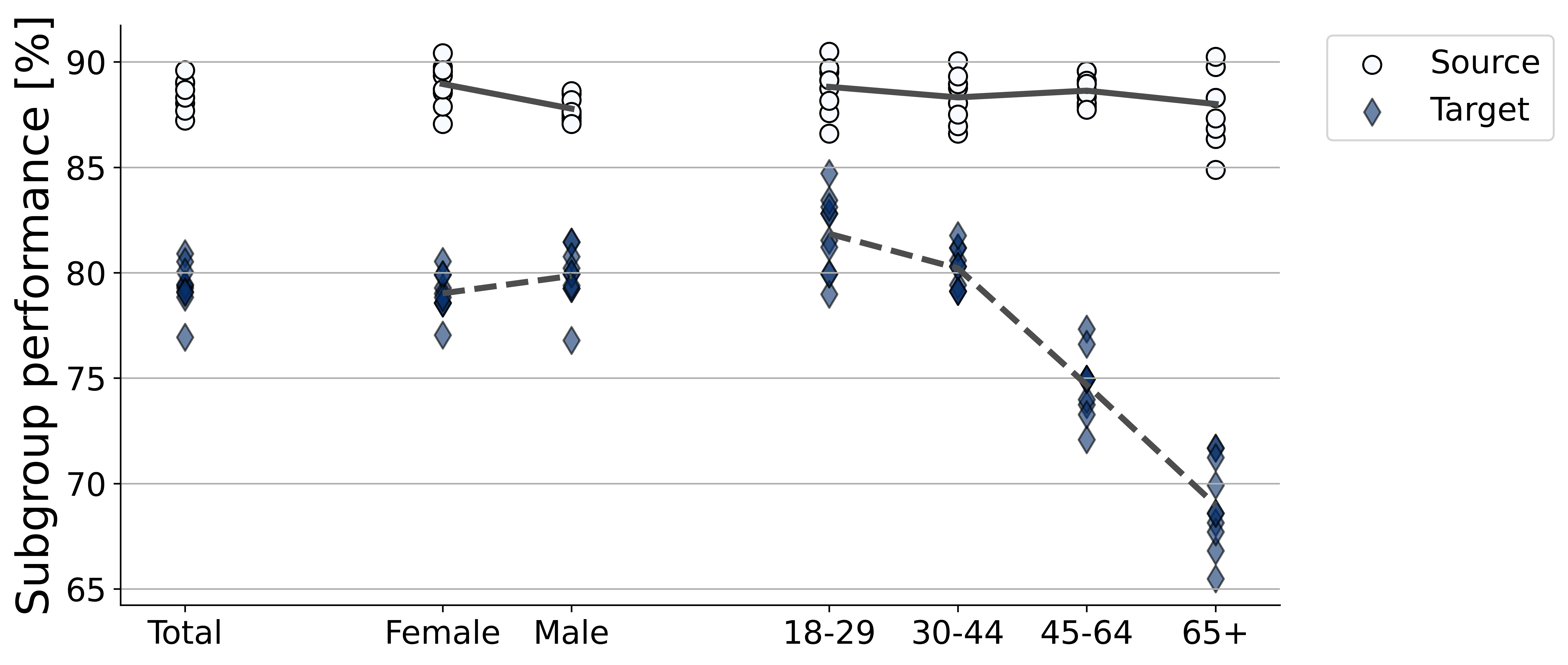
(b) EHR

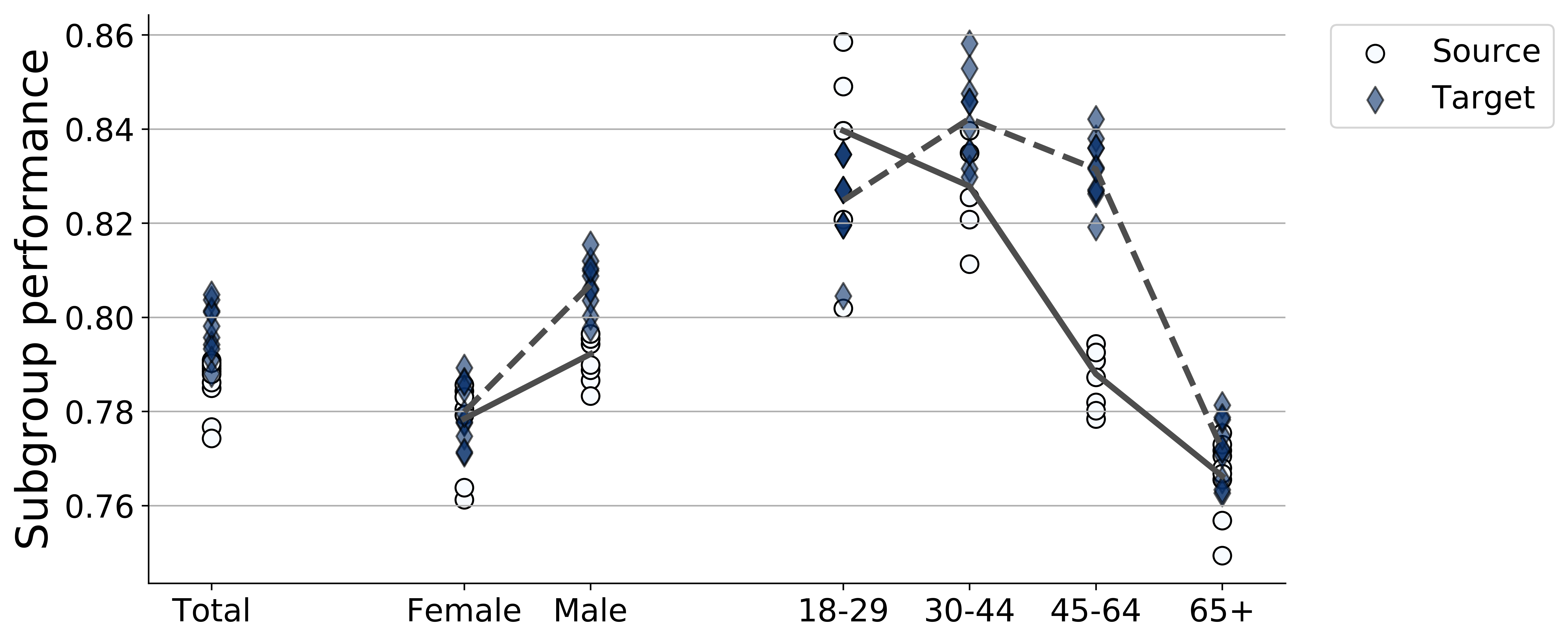
Figure 1: Model performance across subgroups (age and sex) on the source (circles with plain line) and target (diamonds with dashed line). Each marker represents one replicate of the model. (a) Top-3 accuracy (in %) in the dermatology application. (b) Accuracy in EHR.

We assess model performance and fairness across 10 replicates of the model on the source and on the target (Fig. 1). On the source data, the model performs similarly across all subgroups and could reasonably be assessed as ‘fair’. However, the maximum gap between age groups increases starkly on the target (from $1.05\%$ to $12.86\%$).

To understand the failure of fairness transfer in this context, we investigate the structure of the shift by referring to Algorithm 1. We begin by drawing a simplified causal graph $\mathcal{G}$ of the dermatology task at hand (Fig.2(a)). We consider this an anti-causal learning task [63], in which the skin condition label $Y$ is a cause of the input image $X$, and consider demographic information $A$ to be a causal parent of both $X$ and $Y$. We omit variables that are unobserved in either the source or target data.

We now test whether the shift $S$ has direct effects on $A$, $Y$, or $X$. Overall, we find that the shift is compound, and affects all three aspects of the data distribution. We begin with $A$, which comprises age and sex. Because $A$ has no causal parents in our graph (besides, potentially, $S$) we directly assess differences in age and sex across environments using classical tests. Age has a different distribution across the two datasets (see Fig. 2(b)), with the population in the source data being typically younger (median: 40 years old, 25$\%$ quantile: 27, 75$\%$ quantile: 54) than in the target data (median: 44 years old, 25$\%$ quantile: 30, 75$\%$ quantile: 59). Sex distributions are well matched across the source and target. These results suggest a direct effect of $S$ on $A$, and we add this relationship to the causal graph (Fig. 2(a), in purple).

(a)

(b)

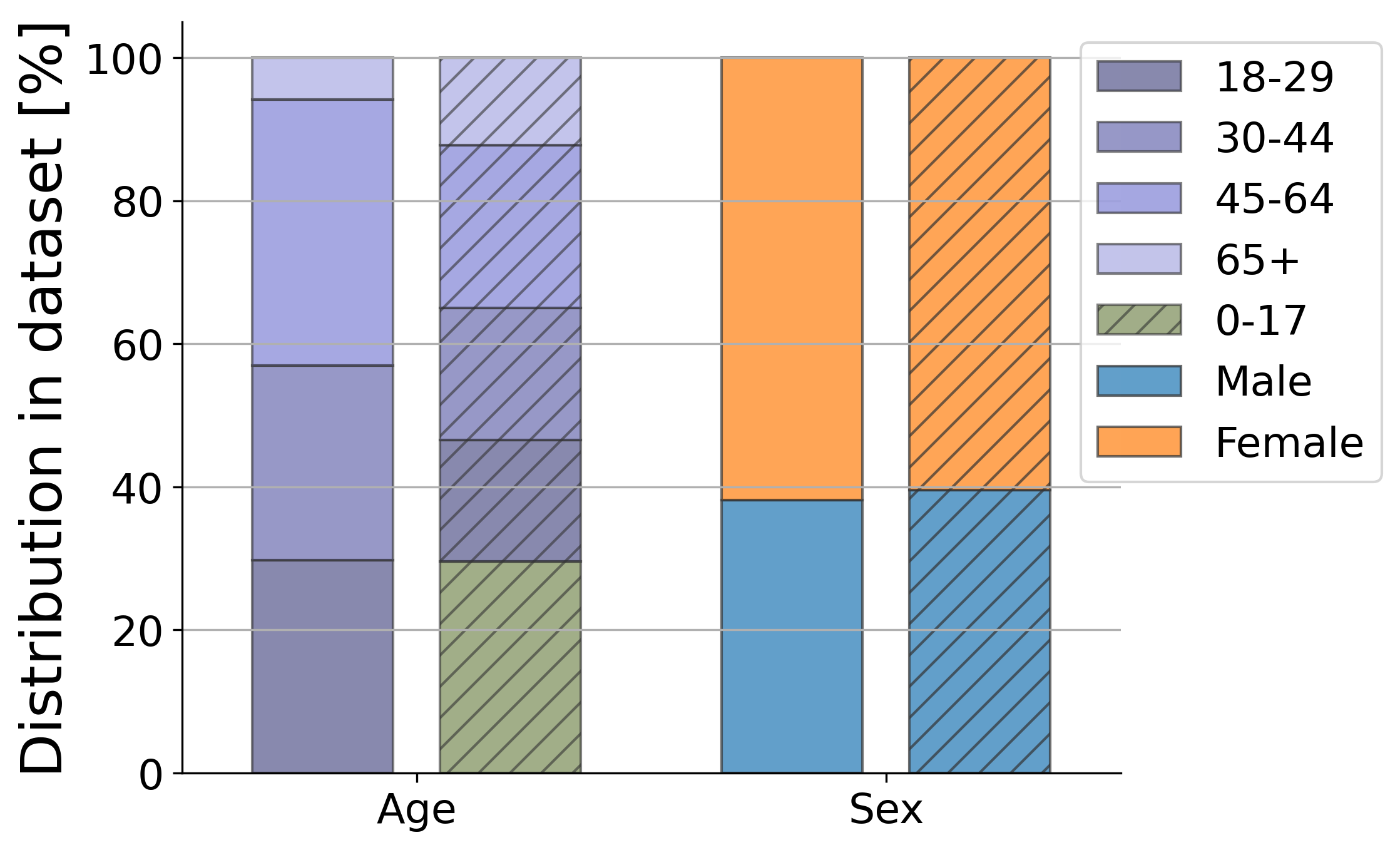
(c)

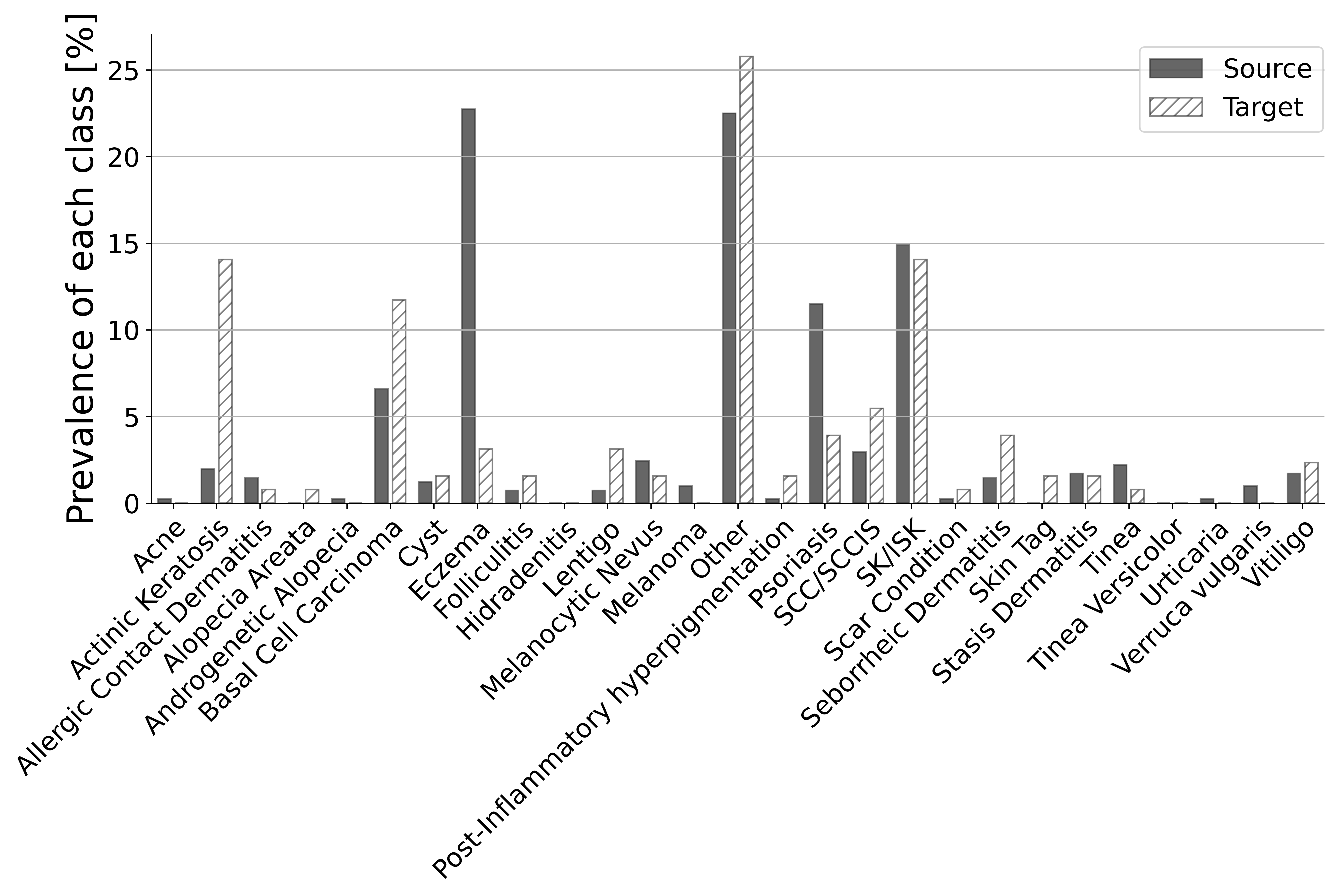
(d)

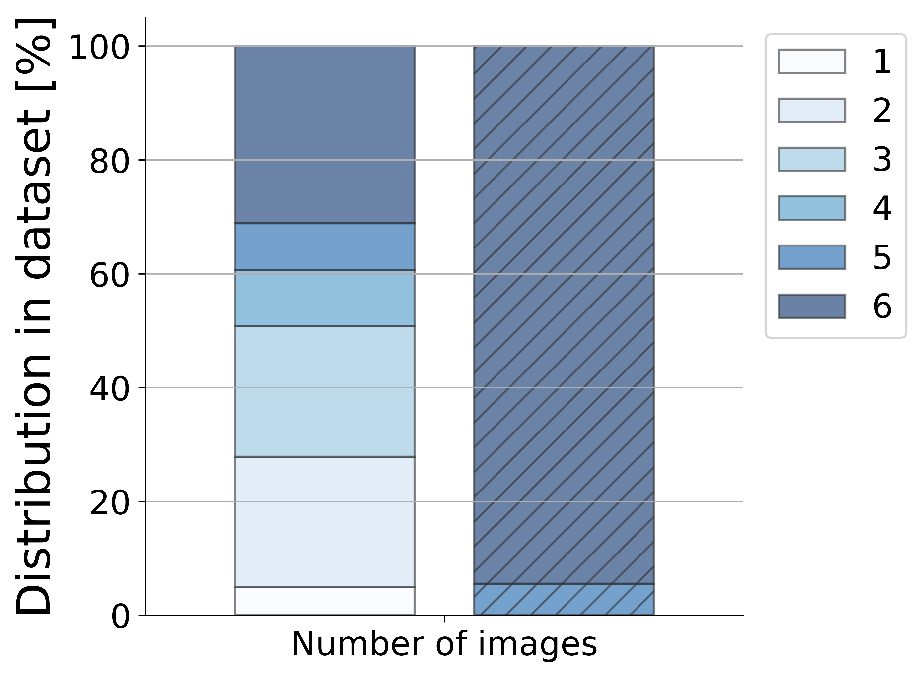
Figure 2: A compound shift in dermatology. (a) Simplified causal structure of the application (see text for variable description). Colored arrows represent statistical dependence as identified by Algorithm 1. (b) Distribution in the source and in the target dataset of the sensitive attributes, computed in terms of percentage of pre-defined subgroups. (c) Prevalence of each condition for female patients over 65 years of age. (d) Distribution of the number of images in cases labelled as ‘SK/ISK’ in older females. Each case includes min. 1, max. 6 images whose embeddings are then averaged. The distributions in the source data are presented on the left, and their corresponding distributions in the target data on their immediate right with a hashed pattern.

We then assess whether $S$ directly affects the labels $Y$. In our graph, $A$ is a causal parent of $Y$, so following our testing strategy in Algorithm 1, we test whether $P(Y\mid A,S=0)=P(Y\mid A,S=1)$. (Recall that conditioning on $A$ isolates the direct effect of $S$ on $Y$.) Using 27 univariate tests (one per condition, [56]), we obtain significant differences between $P(Y\mid A,S=0)$ and $P(Y\mid A,S=1)$ for 3 conditions ($p<0.05$, Bonferroni corrected). Fig.2(c) illustrates the label shift in a specific age and sex subgroup (here females aged 65+, 409 cases in the source, 128 in the target data). We see that the source data includes more cases of ‘eczema’ and ‘psoriasis’ while conditions like ‘actinic keratosis’ and ‘seborrheic dermatitis’ are more represented in the target. These results suggest that the environment also directly affects the labels (orange link in Fig.2(a)).

Finally, we consider whether the features of the images themselves (designated by $X$) are directly affected by $S$. Conditioning on causal parents of $X$, we test whether $P(X\mid Y,A,S=0)=P(X\mid Y,A,S=1)$. We summarize $X$ by training a model $f(X)\rightarrow Y$ on the source, a strategy proposed in Rabanser et al. [56]. Our weighted tests suggest a significant difference between the two distributions ($p<0.05$ corrected on 1 dimension). Fig.2(d) illustrates this difference by computing the number of images per case in the group of older females considered above with cases labelled as ‘SK/ISK’ ( source median: 3, $n=61$, target median: 5, $n=18$). This result suggests the existence of the direct path $S\rightarrow X$ and we add this relationship to the graph (green link in Fig.2(a)).

Based on these results, we observe that all aspects of the data are affected by the environment. Thus, none of the conditional independence conditions for fairness transfer hold in this setting. However, we also see that some conditions might display invariance once controlled for demographics, which suggests possible mitigations that we explore in Section 5. The Supplement includes experimental details and further results on the second target and the joint training.

4.2 Clinical risk prediction from Electronic Health Records

In this application, we predict the clinical outcomes of patients based on EHRs. EHRs record the time series of interactions between a patient and the clinical system (e.g. medication, labs, vitals, …). Distribution shift is a major concern for systems that consume EHR data, which can be heterogeneous across centers [82, 68], and even within a single system [47]. As an example, over half of hospitals in the US with intensive care units (ICUs) only have a single unit where all critically ill patients (medical, surgical, cardiac, etc.) are admitted . Risk scores, such as the Acute Physiology and Chronic Health Evaluation II (APACHE II) score are used to evaluate all critically ill patients, but do not perform equally across clinical subgroups, e.g. underperforming on patients with cardiac disease [55]. It would be desirable to avoid such issues with risk scores constructed through machine learning. We use the open access, de-identified Medical Information Mart for Intensive Care III (MIMIC-III) dataset [30], which consists of data from admissions to ICUs at the Beth Israel Deaconess Medical Center between 2001 and 2012. This clinical system has the benefit of having separate specialized ICUs and allows to assess the generalizability of risk scores estimated in one clinical population to another. Based on clinical input, we consider the Medical ICU (MICU), Surgical ICU (SICU) and Trauma Surgical ICU (TSICU) to be generalist ICUs (source data); whereas the Cardiac Surgery Recovery Unit (CSRU) and Coronary Care Unit (CCU) are specialized ICUs (target data). This split leads to 17,641 patients included in the source dataset and 10,442 patients in the target dataset, after selecting adult patients with a length of stay of minimum one day and with a recorded care unit. Our goal is to obtain a robustly fair model that predicts prolonged ICU stay (i.e. length of stay $>3$ days, as in [78, 54]) using data from the first 24 hours of first ICU admission and a recurrent architecture [72, 73, 61]. The model is trained on $80\%$ of the source data, tuned using a separate split of $10\%$ and tested on the remaining $10\%$. See the Supplement for further details. Noteworthy, the model does not have access to the ‘reason for visit’.

Figure 1(b) shows that the fairness properties of this model, as measured by gaps in subgroup performance, demographic parity (DP) and equalized odds (EO), do not transfer across ICU types. The model displays unfairness w.r.t. age in both datasets (maximum gap $\sim 7\%$, similar DP and EO scores). However, the pattern of unfairness is different in the two datasets, with e.g. the 45-64 years old subgroup being under-served in the source but over-served in the target. The performance gap between sex groups increases from $1\%$ in the source (DP: $0.002\pm 0.002$) to $2.7\%$ (DP: $0.016\pm 0.003$) on the target.

To understand this failure of fairness transfer, we examine the structure of the shift. First, we draw a causal graph for the variables in this problem, building on the work in Singh et al. [67]. Here, we incorporate demographics $A$ as age and self-reported sex, comorbidities $M$ as previous medical history defined by ICD-9 codes [9, 18, 28, 37], observed features $X$ as all labs and vitals, and $Y$ as our prolonged length of stay label. As a more comprehensive feature set leads to better predictive performance [61], we use all 59,351 features at our disposal and add ‘treatments’ $T$ (e.g. medications) to the graph (Fig. 3(a)). In our graph, $S$ represents the ICU unit type that a patient is admitted to.

We now test whether the shift $S$ has direct effects on the variables in this problem using our proposed approach. Beginning with $A$, which has no causal parents, we test whether $P(A\mid S=0)=P(A\mid S=1)$. We estimate the distribution of age and sex in each dataset (Fig. 3(b)). We observe that the population in the source is typically younger than the population in the target (t-test: $p<0.0001$). In addition, the proportion of males in the source and target differ (source: 50%, target: 65%). Therefore, $S\rightarrow A$.

(a)

(b)

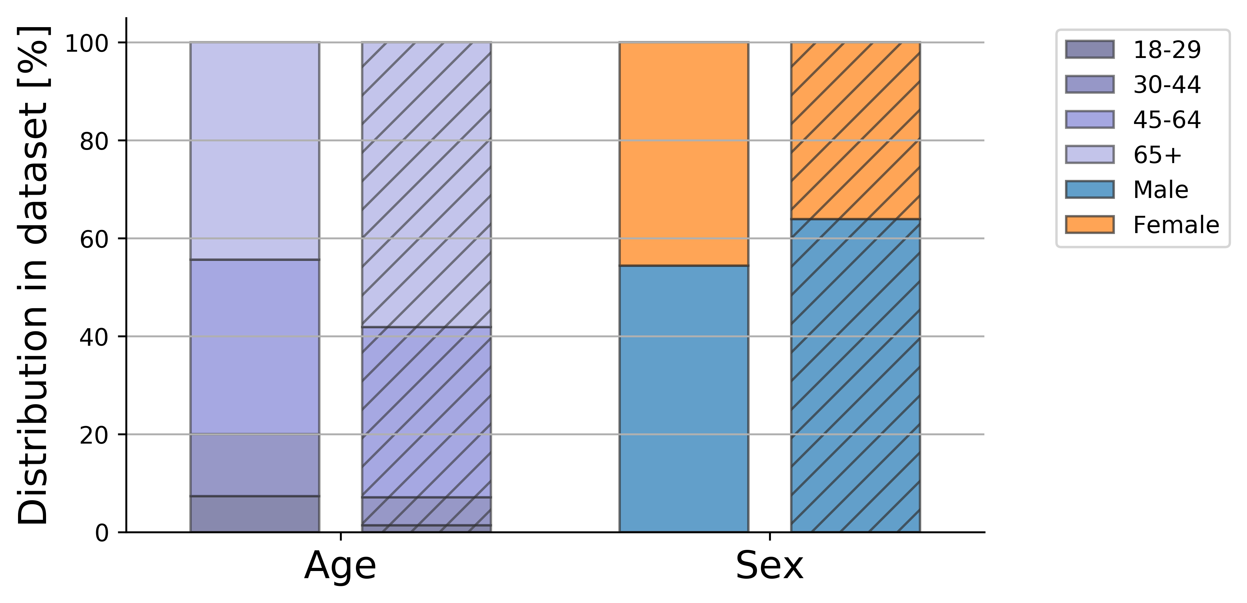
(c)

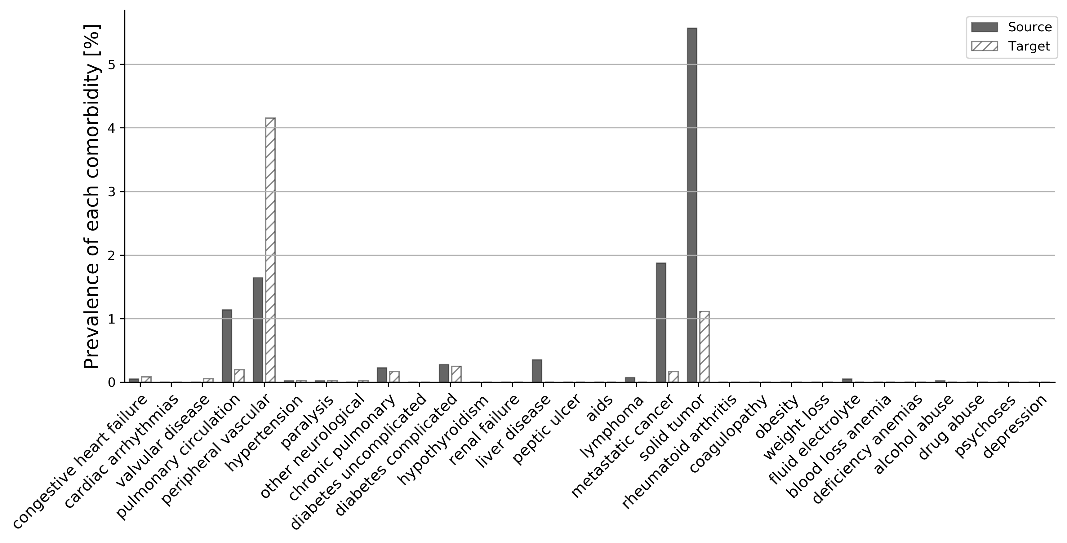
(d)

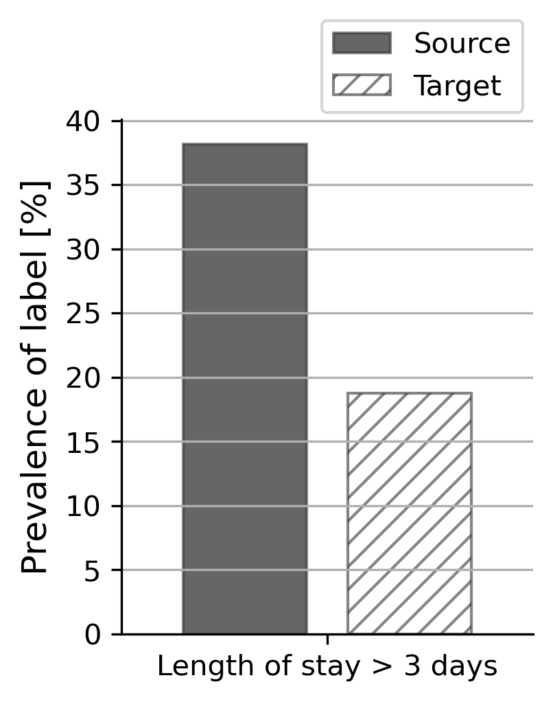
Figure 3: A compound shift in EHR. (a) Causal graph for this application (see text for variable description). Colored arrows represent statistical dependence as identified by Algorithm 1. (b) Distribution of the sensitive attributes, computed in terms of percentage of pre-defined subgroups. (c) Prevalence of comorbidities for male patients over 65 years of age. (d) Prevalence of the label for male patients over 65 with a solid tumor comorbidity and under vasopressors/inotropes. The distributions in the source are represented on the left, and their corresponding distributions in the target on their immediate right with a hashed pattern.

To assess the shift’s effect on comorbidities $M$, we refer to Elixhauser and Vanwalraven scores [21, 74] computed on the source and target data [31]. Figure 3(c) displays the distribution of the 30 comorbidities for older males ($n=3,951$ in source and $n=3,588$ in target). As expected, even after adjusting for the causal parent $A$, patients in the target data have a higher prevalence of comorbidities related to the peripheral vascular system than in the source data and $M\centernot{\mathrel{\perp\mspace{-10.0mu}\perp}}S\,|\,A$ for 5 comorbidities (weighted tests: $p<0.05$, Bonferroni corrected).

We repeat the analysis to assess the direct effect of $S$ on the treatments ($P(T\,|\,A,M,S=0)=P(T\,|\,A,M,S=1):p<0.05$), on the labs and vitals ($P(X\,|\,A,M,T,S=0)=P(X\,|\,A,M,T,S=1):p>0.05$) and on the label ($P(Y|A,M,T,S=0)=P(Y\,|\,A,M,T,S=1):p>0.05$) in the Supplement. Figure 3(d) displays the prevalence of prolonged length of stay for older males with a solid tumor comorbidity and receiving vasopressors/inotropes ($n=55$ in source and $n=16$ in target).

Our results suggest that the shift is compound, i.e. the ICU unit a patient is admitted to changes the relationships between multiple variables in our causal graph. We note that this conclusion is not surprising clinically, given that the environment $S$ is correlated with the reason for their ICU admission, and that this reason for admission (unobserved) is a main driver for all variables. As in the dermatology case, the compound shift leads to multiple paths for $S$ and $A$ to affect the covariates $M$ and $X$ and the label $Y$, explaining the failure of fairness transfer.

5 Mitigation and related work

A variety of fairness, robustness and robustly fair mitigation strategies have been proposed. We contextualize a number of methods in terms of anti-causal and causal learning tasks [63] in the Supplement, and highlight how understanding the nature of the distribution shift can guide mitigation.

Fairness mitigation. Pre-, in- and post-processing techniques for mitigating unfairness have been proposed [see 5, 48, for overviews]. Fairness metrics and mitigation techniques currently used in real-world applications are typically evaluated on a single learning task or data distribution [e.g. 90, 2, 79, 54, 11]. More similar to our settings, the work by Creager et al. [15] addresses fairness in dynamical systems, although only for low-dimensionality variables. Based on our causal framing, applying fairness mitigations in the source domain could potentially aid in fairness transfer by cutting some edges in the underlying CBN [75]. However, fairness mitigation on the source only leads to provable fairness transfer in specific settings, i.e. mostly when the shift is demographic (Supplement).

Based on this analysis, performing fairness mitigation in the presence of a compound shift would fail to provide a fair result on the target. Considering the applications above, a reasonable option would be to perform fairness mitigation for the EHR task based on age. We perform post-processing of the predictions to enforce either demographic parity or equalized odds across age subgroup using the method in Alabdulmohsin and Lučić [3]. This results in a decrease in demographic parity to value $10^{-5}$ in the source, but to (slightly) increase to value $0.078\pm 0.025$ in the target data. Similarly, equalized odds decrease to value $10^{-5}$ and the gap in model accuracy between groups is reduced from 7% to 0.8% (Fig. 4) in the source, but increases from $0.05\pm 0.008$ to $0.16\pm 0.04$ on the target data, and the gap between age groups increases to 11.4%. We therefore observe that mitigating for either demographic parity or equalized odds on the source leads to no improvement, or even worsening of the fairness properties on the target, as predicted by our analysis.

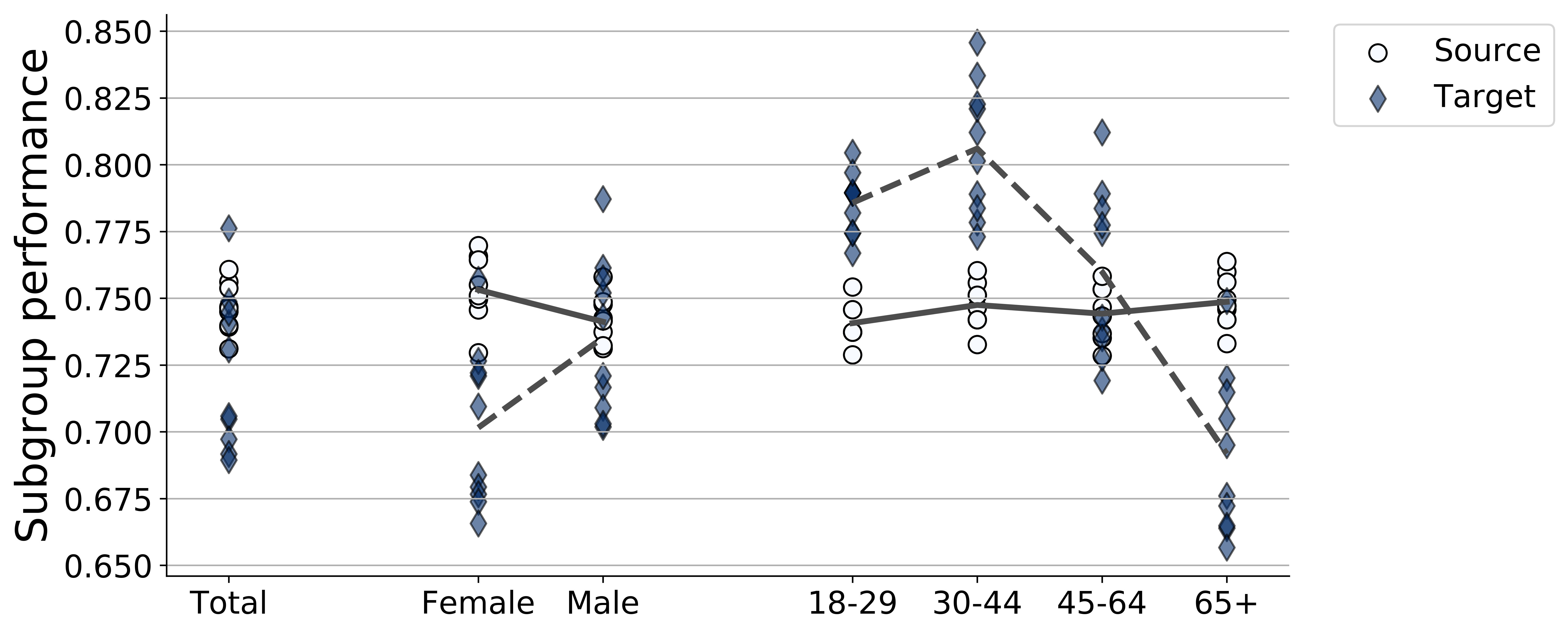
Figure 4: EHR model accuracy across subgroups after post-processing of the predictions for equalized odds based on age.

Robustness mitigation: Relations between robustness guarantees and individual and group fairness have been studied in [85, 46, 83, 84] and [75] respectively. [1, 16, 88] have investigated the relationship between fairness and distribution shift experimentally by studying how robustness mitigation strategies affect fairness metrics. These works do not provide provable robustly fair models.

Robustly fair mitigation. Work explicitly investigating fairness properties under distribution shift can mostly be divided into methods that provide a priori guarantees or bounds [e.g. 64, 67, 70] and methods that adapt to the new distribution [e.g. 13, 49, 69, 89, 32, 19, 71].

Recent work by Singh et al. [67] suggests a straightforward mitigation with guarantees, based on selecting features that satisfy the fairness transfer criteria outlined in Section 2. However, this approach is limited under compound shifts with complex data. Most notably, it cannot be used in cases where there is a label shift ($S\rightarrow Y$). However, even when there is no label shift, under compound shifts the criteria for feature selection can yield a trivial predictor where no observed variables can be used. This is the case in our EHR example under the joint causal graph in Fig. 3(a). We discuss the applicability of [67] across different causal scenarios in the Supplement. In addition, feature selection approaches are more suited for semantic features and, while it is technically feasible, would not lead to insightful results in non-semantic features such as pixels. In computer vision, masking has been used previously as an approximation to feature selection to constrain the learning towards specific areas of the image [59, 66]. While this technique has shown some promise with chest x-rays [76], it is impractical due to the additional requirement of a mask for all training images. In addition, it increases the ratio of signal of interest compared to undesirable signal, but does not exclude such signals and comes with no guarantee.

Another line of work considers adapting transfer learning and meta-learning algorithms to consider fairness constraints and therefore ensure generalization to new tasks also in terms of fairness [13, 49, 69, 89]. Specifically, Coston et al. [13] modify the standard approach to transfer learning under covariate shift by adding a constraint to the weight learning objective that enforces closeness between all pairs of protected groups. Schumann et al. [64] provide bounds on fairness transfer by adding adversarial heads on both the in-source attribute $A$ and the environment $S$. When we cast this work into our causal framework, we notice that it would provide a robustly fair model under an exclusive covariate shift in an anti-causal learning task. Slack et al. [69] propose meta-learning with a regularizer that imposes demographic parity or equalized odds to improve the transfer of fairness. The method requires a small set of labelled target data (K-shot learning) and multiple tasks, and comes with no guarantees. Work on fine-tuning and transfer learning [49, 89] leverages task similarity to learn fair representations that provably generalize to unseen tasks, similarly requiring a small set of labelled target data. Importantly, these methods generate one tuned model per environment, which is not suitable for all real-world deployments of ML. It is also unclear whether these techniques could handle more complex tasks, e.g. predictions from sparse multivariate timeseries as in the case of EHR.

Shift detection. Many methods exist to detect covariate shift [e.g. 42, 8] or label shift [39, 25]. They however often rely on the assumption that other variables are not affected by the shift. For instance, Lipton et al. [39] relies on the assumption that $X\mathrel{\perp\mspace{-10.0mu}\perp}S\,|\,Y$. On the other hand, Slack et al. [69] introduce a technique to identify mean shifts that could lead to unfairness. While the method is an interesting step towards ‘fairness transfer warnings’, this strategy does not allow to guide the selection of mitigation. Recently, Singh et al. [68] investigate differences in source and target distributions using squared maximum mean discrepancy [27], but do not take the causal structure into account. To differentiate direct from indirect effects of $S$ on variables $U$, they perform causal inference and visually inspect the obtained graph. This method can only be applied to low-dimensionality datasets.

6 Discussion

In this work, we applied statistical tests within a joint causal framework [45] to better understand failures of fairness transfer across distribution shift. Our approach tests for direct effects of the environment on every random variable in a task. We use this technique to characterize distribution shifts that result in two real world failures of fairness transfer in the healthcare domain. We show that this knowledge can then guide the choice of an appropriate mitigation strategy, when applicable.

Our work highlights real-world challenges that prevent the development of robustly fair models. Given that each task leads to different complexities in terms of causal graph, expected shifts, and fairness requirements, these findings support looking beyond purely algorithmic solutions. Considering the whole ML pipeline, we can re-interpret the remedies discussed in Chen et al. [10] for fairness transfer:

1. Problem selection. Consider focusing on tasks with lower anticipated harms or clinical/policy safeguards against ML unfairness.

2. Data collection. Consider early data collection from anticipated deployment environments in which distribution shifts are suspected. This would allow to perform (conditional) independence tests to guide further mitigation.

3. Outcome definition. Consider intermediate outcomes for which unfairness under distribution shift might be less consequential (e.g. image segmentation compared to diagnosis).

4. Algorithm development. Based on (2), some strategies can be used if their assumptions are satisfied. In addition, in the present work we used a causal framework. However, techniques that are not easily cast into this framework exist. For instance, manual feature engineering has been used to improve the robustness of EHR models to distribution shift [47]. While this work has not evaluated the fairness of the model in the source and target distributions, we believe that feature engineering might be a promising avenue to enforce specific inductive biases during learning while reducing the risks of distribution shifts. We however note that our work does not assess the impact of model architecture or different training strategies, which might lead to compounded bias and/or poor generalization.

5. Post-deployment. Further safeguards may be envisaged to safely deploy ML systems, e.g. with a prospective observational (non-interventional) integration [24]. Transfer learning or retraining with site-specific updates might then be considered as necessary prior to interventional deployment. Finally, those deployments may be accompanied with robust post-market surveillance to continuously monitor fairness.

Limitations and future work. The power of our diagnosis method depends on the number and quality of the samples. Therefore, it should be perceived as displaying potentially problematic aspects of the data, rather than assessing invariant features. This is a common limitation in shift detection [39] and mitigation [67]. Furthermore, the data at hand usually represents a set of proxies for the underlying variables. Therefore, even if a shift seems to satisfy some invariance assumptions, there are no sharp guarantees [23]. This is especially true for demographic factors: features such as ethnicity, age or sex only approximate sensitive attributes. We are also limited by which factors are observed across all environments and cannot assess changes in unobserved variables (e.g. social determinants of health).

While our work covers different types of shift, future work should investigate further sources of shift and biases, such as sampling biases or missingness [7, 88]. In addition, extending the testing strategy to compare multiple (discrete or continuous) versions of the environment $S$ would be valuable.

By specifying causal graphs for each problem, we make assumptions about the relationships between variables. These assumptions might not represent the true underlying data generation process. In addition, the effects of $A$ could potentially be divided into ‘fair’ and ‘unfair’ effects, as proposed in [12, 44]. For real-world applications, further assumptions were made, e.g. considering the silver standard label in dermatology as a good approximation for the gold standard label (hence an anti-causal task) [7]. The value of these graphs is purely illustrative and should not be considered for medical applications without validation.

In terms of metrics, we have focused mostly on demographic parity and equalized odds, due to their recent causal grounding [75]. Different metrics might, however, be affected differently, and it is possible that some metrics are more or less ‘sensitive’ to distribution shift. Similarly, different fairness mitigation strategies might be affected differently by distribution shift, although none provides guarantees under distribution shift. We also note that ‘fairness’ in the healthcare domain is an active discussion, and that equalized odds or demographic parity metrics do not consider factors such as social determinants of health or health equity. As discussed in [54], considering human elicited metrics might be an avenue forward. Similarly, ‘fairness’ might change depending on the context [62] and different metrics might be relevant in different environments.

1. For all authors…

   1. Do the main claims made in the abstract and introduction accurately reflect the paper’s contributions and scope? [Yes] We clearly describe that our main contribution is to provide a method that assesses the structure of a distribution shift.

   2. Did you describe the limitations of your work? [Yes] Please see the separate subsection in the Discussion.

   3. Did you discuss any potential negative societal impacts of your work? [Yes] In the limitation section, we discuss how algorithmic fairness is a set of mathematical formulations and does not ensure fairness in outcomes or health equity.

   4. Have you read the ethics review guidelines and ensured that your paper conforms to them? [Yes]

2. If you are including theoretical results…

   1. Did you state the full set of assumptions of all theoretical results? [Yes] Assumptions are most relevant for our statistical tests and the simplified causal graphs we propose. We clearly mention these in the text, as well as in the discussion.

   2. Did you include complete proofs of all theoretical results? [N/A]

3. If you ran experiments…

   1. Did you include the code, data, and instructions needed to reproduce the main experimental results (either in the supplemental material or as a URL)? [Yes] The main contribution of this work is the statistical tests. Algorithm 1 and the Supplement provide detailed instructions to re-implement the approach, including practical tips.

   2. Did you specify all the training details (e.g., data splits, hyperparameters, how they were chosen)? [Yes]

   3. Did you report error bars (e.g., with respect to the random seed after running experiments multiple times)? [Yes] We report our results on 10 seeds of each model.

   4. Did you include the total amount of compute and the type of resources used (e.g., type of GPUs, internal cluster, or cloud provider)? [Yes] Computational resources are discussed in the Supplement.

4. If you are using existing assets (e.g., code, data, models) or curating/releasing new assets…

   1. If your work uses existing assets, did you cite the creators? [Yes] We cite the creators of both healthcare datasets and refer to the code we used or took inspiration from throughout the text and in the Supplement.

   2. Did you mention the license of the assets? [Yes] Where available.

   3. Did you include any new assets either in the supplemental material or as a URL? [No]

   4. Did you discuss whether and how consent was obtained from people whose data you’re using/curating? [No]

   5. Did you discuss whether the data you are using/curating contains personally identifiable information or offensive content? [Yes] See Supplement.

5. If you used crowdsourcing or conducted research with human subjects…

   1. Did you include the full text of instructions given to participants and screenshots, if applicable? [N/A]

   2. Did you describe any potential participant risks, with links to Institutional Review Board (IRB) approvals, if applicable? [Yes] We discuss the ethical reviews for the dermatology datasets in the Supplement.

   3. Did you include the estimated hourly wage paid to participants and the total amount spent on participant compensation? [N/A]

Appendix

Appendix A Methods

In this section, we provide further details on the methods, including the mathematical definitions of our metrics and an in-depth description of our testing procedure.

A.1 Fairness metrics

Our work focuses on statistical group definitions of fairness [5]. In particular, we frame the discussion around demographic parity in which the model’s output is statistically independent of the sensitive attribute, i.e. $f(X^{\prime})\,\mathrel{\perp\mspace{-10.0mu}\perp}\,A$, and equalized odds in which the independence holds conditionally on the outcome, i.e. $f(X^{\prime})\,\mathrel{\perp\mspace{-10.0mu}\perp}\,A\,|\,Y$. In the experiments, these metrics are computed for binary tasks. We also compute the gap in subgroup accuracy. For all fairness metrics, the lower, the better.

We define demographic parity for a predictor $f$ as [20, 86, 43, 3]:

$$\max_{a\in\mathcal{A}}\,\mathbb{E}_{\mathbf{x}}[f(\mathbf{x})\,|\,A=a]\,-\,\min_{a\in\mathcal{A}}\,\mathbb{E}_{\mathbf{x}}[f(\mathbf{x})\,|\,A=a]$$ (1)

Equalized odds is computed in a similar fashion by conditioning on the positive and negative classes, taking the average of the discrepancies across classes.

Subgroup performance is computed as the accuracy (top-1 or top-3 in the case of dermatology, accuracy for EHR) within each subgroup. When the sensitive attribute is non-binary, we compute the maximum difference between any pair of subgroups.

A.2 Causal framework

A Bayesian network [14, 35, 51, 52] is a directed acyclic graph (DAG) ${\mathcal{G}}$ whose nodes $X^{1},\ldots,X^{D}$ represent random variables and links express statistical dependencies among them. Each node $X^{d}$ is associated with a conditional probability distribution (CPD) $p(X^{d}\,|\,{\text{pa}}(X^{d}))$, where ${\text{pa}}(X^{d})$ denote the parents of $X^{d}$, namely the nodes with a link into $X^{d}$. The joint distribution of all nodes is given by the product of all CPDs, i.e. $p(X^{1},\dots,X^{D}\,|\,{\mathcal{G}})=\prod_{d=1}^{D}p(X^{d}\,|\,{\text{pa}}(X^{d}))$. This function is assumed to be invariant across distributions. A path from $X_{i}$ to $X_{j}$ is a sequence of linked nodes starting at $X_{i}$ and ending at $X_{j}$. A path is called directed if the links point from preceding towards following nodes in the sequence. A node $X_{i}$ is an ancestor of a node $X_{j}$ if there exists a directed path from $X_{i}$ to $X_{j}$. In this case, $X_{j}$ is a descendant of $X_{i}$. We say that a set of nodes {$X^{i},\ldots,X^{j}$} d-separates two random variables $U$ and $W$ if $U\mathrel{\perp\mspace{-10.0mu}\perp}W\,|\,{\{X^{i},\ldots,X^{j}\}}$. A causal Bayesian network is a Bayesian network in which a link expresses causal influence rather than statistical dependence. In causal Bayesian networks, directed paths are called causal paths.

A.3 Assessing the causal structure of shifts

A.3.1 General Strategy

To assess the causal structure of a shift, we examine whether there is a direct effect of the shift $S$ on a focal variable $U$. This requires controlling for all other pathways by which $U$ may depend on $S$. To do this, we select a set of variables $\mathbf{V}$ such that {$\mathbf{V}$} blocks all indirect paths from $S$ to $U$. We then test the following equality in conditional distributions: $P(U\mid\mathbf{V},S=0)=P(U\mid\mathbf{V},S=1)$ almost everywhere.

To test the equality of conditional distributions, we reduce the problem to testing whether the means of the two marginal distributions of $U$ are equal when the distributions of the background variables $\mathbf{V}$ are adjusted to follow the same distribution. Using observed data from environments $S=0$ and $S=1$, we can perform such an apples-to-apples comparison using importance weighting. In particular, for any distribution $\pi(\mathbf{V})$,

$$P(U|\mathbf{V},S=0) =P(U|\mathbf{V},S=1)\quad\text{for almost all }\mathbf{V}\quad\implies$$ (2)

$$\int E[U\mid\mathbf{V}\mid S=0]\pi(\mathbf{V})d\mathbf{V} =\int E[U\mid\mathbf{V}\mid S=1]\pi(\mathbf{V})d\mathbf{V}\quad\implies$$ (3)

$$E\left[\frac{\pi(\mathbf{V})}{P(\mathbf{V}\mid S=0)}E[U\mid\mathbf{V}\mid S=0]\mid S=0\right] =E\left[\frac{\pi(\mathbf{V})}{P(\mathbf{V}\mid S=1)}E[U\mid\mathbf{V}\mid S=1]\mid S=1\right]\implies$$ (4)

$$E\left[\frac{\pi(\mathbf{V})}{P(\mathbf{V}\mid S=0)}U\mid S=0\right] =E\left[\frac{\pi(\mathbf{V})}{P(\mathbf{V}\mid S=1)}U\mid S=1\right]$$ (5)

Define the weights $w_{0}(\mathbf{V}):=\frac{\pi(\mathbf{V})}{P(\mathbf{V}\mid S=0)}$, and $w_{1}(\mathbf{V}):=\frac{\pi(\mathbf{V})}{P(\mathbf{V}\mid S=1)}$. This result shows that we can test the equality of the conditional distributions by testing the implication that the mean of weighted outcomes is the same.

This leaves a degree of freedom for choosing the test distribution $\pi(\mathbf{V})$ on which the conditional distributions will be compared. This distribution then determines the weighting scheme that will be used. We define $\pi(\mathbf{V})$ to be a constant, i.e., uniform. Then the weights are

$$w_{0}(\mathbf{V})\propto P(\mathbf{V}\mid S=0)^{-1}\quad\text{and}\quad w_{1}(\mathbf{V})\propto P(\mathbf{V}\mid S=1)^{-1}.$$

This weighting scheme is known as inverse probability weighting or IPW [58, 29], and is a popular choice. We however note that other weighting schemes could be considered, e.g. overlap weights [38] or permutation weighting [4].

In practice, the likelihoods $P(\mathbf{V}\mid S=s)$ used to define the weights need to be learned from data. Usefully, because of how the weights are normalized, the likelihoods can be replaced with classification scores that estimate $P(S=s\mid\mathbf{V})$, leading to estimated weights $\hat{w}_{0}$ and $\hat{w}_{1}$. The choice of the classifier can be informed by the expected relationships between {$\mathbf{V}$} and $S$: for instance, logistic regression can be considered in the case of simple relationships, while more expressive classifiers such as gradient boosted trees can be considered in the case of non-linear relationships [4]. As discussed in Arbour et al. [4], all classifiers are tuned (C for logistic regression, number of trees, tree depth and learning rate for boosted trees) in a cross-validation setup.

We then use a standard t-test to test the null hypothesis

$$H_{0}:E[\hat{w}_{0}U\mid S=0]-E[\hat{w}_{1}U\mid S=1]=0.$$

To decrease the variance in the obtained t-statistics, we bootstrap the weighting and testing procedure. The final p-value associated with $H_{0}:P(U\mid\mathbf{V},S=0)=P(U\mid\mathbf{V},S=1)$ is the p-value of a two-sided $\mathcal{Z}$-test on the t-statistics obtained from each bootstrap.

Observations and tips From our observations, we note that it is best to allocate the largest available sample to estimate the likelihood ratio, compared to performing the final statistical test. We also observed that gradient boosted trees can lead to extreme weights in some cases. This results in an increased variance and non-significant results. We therefore clipped the weights to a maximum of 10 (arbitrary choice) to mitigate this effect.

A.3.2 Testing with High-Dimensional $U$

If $U$ has low dimensionality, Rabanser et al. [56] show that multiple one-dimensional tests can be used with correction for multiple comparisons (here Bonferroni). On the other hand, if $U$ has higher dimensionality (e.g. an image), summaries of $U$ can be constructed and the test can be performed on these lower-dimensional summaries. The validity of this approach follows from the fact that if the conditional distributions of $U$ are the same, then so will the conditional distributions of any summary $f(U)$. The trade-off is that the test loses all power to detect distributional differences that are compressed out by the summary $f(U)$, or to highlight specific dimensions in $U$ that are more or less affected by $S$. To define a summary that is relevant to the problem, Lipton et al. [39] suggest defining $f(U)$ to be the output of a model the predicts some variable of interest (say the outcome $Y$) using $U$. As reported in Rabanser et al. [56], other summarizing techniques could be considered.

A.3.3 Sanity checks with engineered shifts

We assess the specificity and sensitivity of our testing procedure (see Algorithm 1) using engineered shifts on the dermatology data. To estimate Type I error, we compare the source data to itself, which should lead to all variables being independent of the environment. More specifically, we select $10,000$ random samples from the dataset to compute the weights, and another $1,000$ random samples to apply the weights on and perform the weighted test. These sets are boostrapped 100 times (separately for the source and target sets) and we assess the proportion of false positives that is obtained for each variable $U$. We expect that we will obtain $~{}5\%$ of false positives, as defined by our hypothesis testing threshold. As we do not expect any relationship between {$\mathbf{V}$} and $S$, we use a logistic regression to estimate $P(S=s\mid\mathbf{V})$.

When comparing $P(Y\mid A,S=0)$ to $P(Y\mid A,S=1)$, we observe that the accuracy of the classifier mirrors the chance level of $50\%$ and that the proportion of false positives varies between $2$ and $8.5\%$ (Figure 5(a)). Similarly, comparing $P(X\mid Y,A,S=0)$ to $P(X\mid Y,A,S=1)$ when using a model $f(X)\rightarrow Y$ to summarize $X$ leads to a proportion of false positives between 2 and $7\%$ (Figure 5(b)).

As the number of samples used to compute the weights is an important component of our testing approach, we repeat the process while varying the number of samples from 100 to 5,000. Figure 5(c) displays that the variance on Type I error (here across conditions) decreases when the number of samples to fit the $P(S=s\mid\mathbf{V})$ classifier increases.

(a)

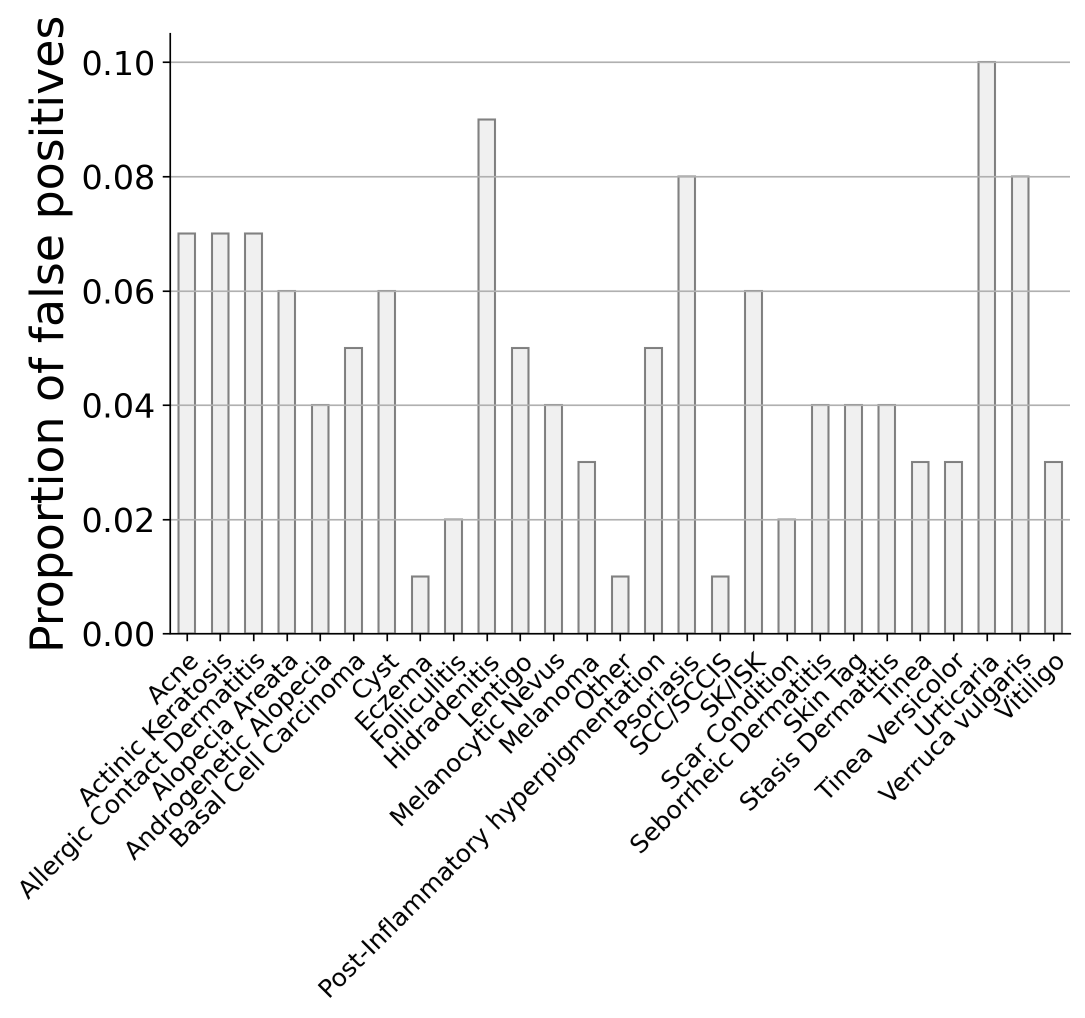
(b)

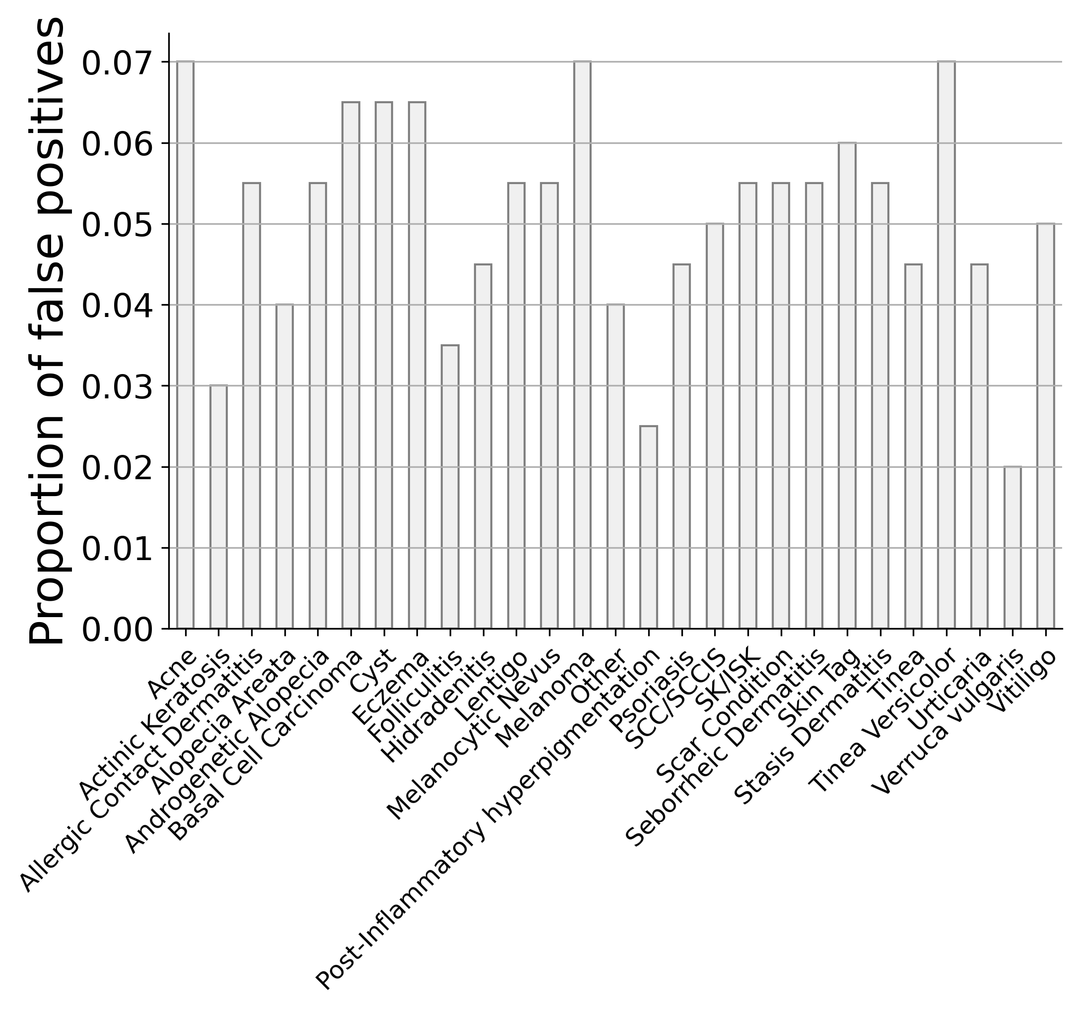
(c)

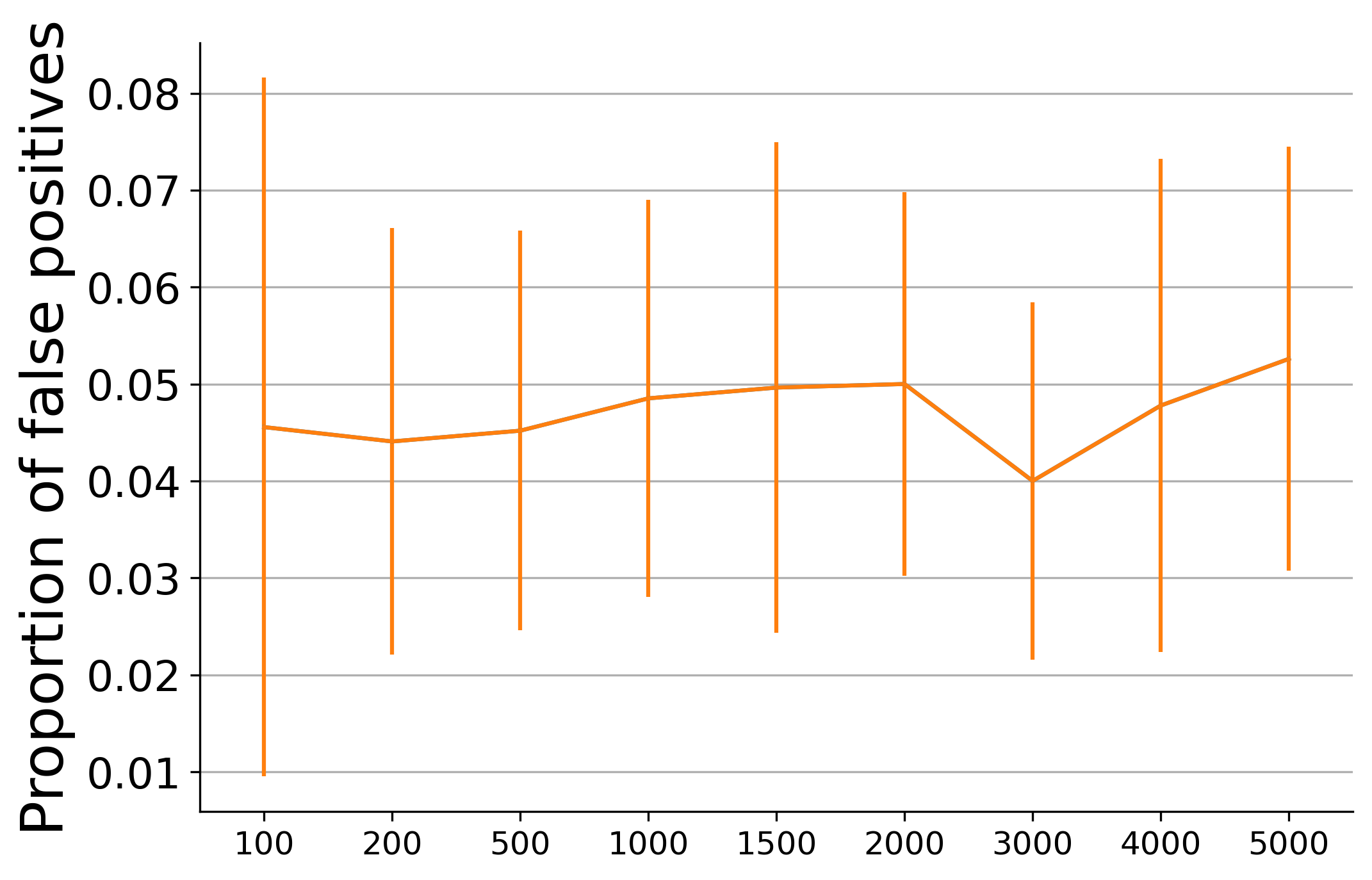
Figure 5: Proportions of false positives when comparing the source data to itself. (a) $P(Y\mid A,S=0)$ vs $P(Y\mid A,S=1)$. (b) $P(X\mid Y,A,S=0)$ vs $P(X\mid Y,A,S=1)$. (c) $P(Y\mid A,S=0)$ vs $P(Y\mid A,S=1)$ when varying the number of samples to estimate $P(S\mid\{\mathbf{V}\})$. In this case, the results are averaged across conditions (with standard deviation).

To assess sensitivity, we then engineer a shift on the data that discards samples based on their age and condition (here Acne). More specifically, we subsample data in order to decrease the bias for younger age in the Acne condition, leading to an increase in age for Acne samples of approximately 10 years. Given that Acne is one of the most prevalent conditions in the dataset, we expect a significant change on age, as well as on $Y$. On the other hand, the images are not modified and hence $P(X\mid Y,A,S=0)$ and $P(X\mid Y,A,S=1)$ should not display significant changes.

We observe a significant change in age between $S=0$ and $S=1$. There is no significant effect of $S$ on other demographic factors. We do observe a direct effect of $S$ on $Y$, with a strong effect on Acne as expected. On the other hand, no tests display significant differences when comparing $P(X\mid Y,A,S=0)$ with $P(X\mid Y,A,S=1)$. This latter result was obtained with both a logistic regression and gradient boosted trees (given the more complex relationship between age and Acne). Therefore, the testing approaches produces a causal graph that mirrors the graph used to engineer the shift, and our procedure is considered faithful.

Finally, we randomly shuffled the labels $y_{k}$ across the 27 conditions, for each case independently. At the population level, this results in a change in $P(Y)$. As expected, there was no effect of $S$ on $A$. For $Y$, we observed significant differences in $P(Y\mid A,S=0)$ and $P(Y\mid A,S=1)$ for 19 conditions out of 27 (Bonferroni corrected). Thanks to the correction, and given that the images were not modified, there are no significant differences between $P(X|Y,A,S=0)$ and $P(X|Y,A,S=1)$.

Overall, our tests are sensitive enough to detect the presence of changes on the affected dimensions, while not displaying an excessive amount of false positives.

Appendix B Causal framing of related works

In this section, we review how various transferable fairness approaches that have been proposed in the literature interact with different causal structures of domain shift depicted in Figures 6 and 7. We assume the same sensitive attributes $A$ in the source and target environments, and consider different relationships between the environment and other variables. As in [7, 75], we split the analysis into causal or anti-causal prediction tasks [63]. A prediction task is causal if the features $X$ are causes of the outcome $Y$, and anti-causal if the outcome $Y$ is a cause of the features $X$. Many risk prediction problems are causal, where risk factors may cause an adverse outcome, while many diagnostic problems are anti-causal, where the underlying disease may cause symptoms [7].

A takeaway from this review is that most methods are tailored to particular restricted shift structures, and their useful properties can break down under compound shifts.

B.1 Anti-causal prediction tasks

First, we consider anti-causal prediction tasks, in which the outcome $Y$ is a direct cause of the features $X$, and that the sensitive attribute $A$ is a direct cause of $X$ and $Y$ (the reality will likely be more complex and involve other variables in the paths (observed or not)). The assumption that $A$ is a cause of $X$ and $Y$ is a reasonable approximation in healthcare settings: e.g. on average, skin images from men are more hairy than those of women, breasts are visible in chest x-rays, and comorbidities are different across sexes and age ranges. Sensitive attributes can also be related to the label, as prevalence can vary across subgroups (e.g. baldness is more prevalent in older patients) and some conditions might present differently across attributes (e.g. a heart attack in men vs women).

In this context, we consider strategies for learning robustly fair models under exclusive demographic, exclusive covariate, exclusive label and compound distribution shift scenarios represented in the causal graphs of Fig. 6:

(a)                              (b)                              (c)                              (d)

Figure 6: Causal graphs under different distribution shifts when considering an anti-causal prediction task. (a) Exclusive demographic shift where the demographics $A$ are directly affected by $S$. (b) Exclusive covariate shift where the $X$ is directly affected by $S$. (c) Exclusive label shift where $Y$ is directly affected by $S$. (d) Compound shift given by the combination of demographic, covariate, and label shifts.

a) Exclusive demographic shift. In Fig. 6(a), we consider an exclusive demographic shift through the direct path $S\rightarrow A$. In this case, the effects of $S$ on $Y$ and $X$ are intercepted by $A$. Therefore, training a fair model based on $X$ (either via imposing equalized odds [67] or counterfactual invariance with respect to $A$ [75]) leads to a robustly fair model.

b) Exclusive covariate shift. In Fig. 6(b), we consider an exclusive covariate shift through the direct path $S\rightarrow X$. In this case, there are multiple causal arrows into $X$ that need to be addressed: $A\rightarrow X$ for fairness, and term $S\rightarrow X$ for robustness to distribution shift. In the case where some labeled target domain data is available, Schumann et al. [64] implement separate independence regularizers to address each path, and demonstrate its effectiveness in settings that match this causal structure. In the fully unlabeled domain adaptation case, the shift is harder to account for. For example, the set of features that satisfy the selection criteria of Singh et al. [67] would only include $A$, leading to a predictor that relies solely on demographics data (Sec. B.3).

c) Exclusive label shift. Lipton et al. [39] propose a technique to detect an exclusive label shift, as well as mitigate it through reweighting, requiring unlabelled target data. This technique can be used in addition to a fairness mitigation technique to lead to a robustly fair model.

d) Compound shift. Such a shift leads to multiple factors being affected by $S$, and current techniques would either be ineffective or degenerate to the trivial predictor. While Fig. 6(d) represents the worst case scenario, even simpler combinations of shifts would lead to similar results in practice. For instance, adding a correlation between $S$ and $A$ to Fig. 6(b) leads to a compound shift. In this specific case, mitigation might be possible by taking all intersections of $A$ and $S$ when using [64]. In practice, if the attribute or the shift have multiple discrete values, this will quickly become intractable, especially if distribution matching needs to be applied within each mini-batch. When considering feature selection, [67] would return an empty set for both equalized odds or demographic parity, leading to a trivial predictor. (Partial) mitigation might be obtained through the use of an adaptation technique as proposed in [69, 49].

B.2 Causal prediction tasks

We repeat the analysis above for the simplest causal prediction task in which $X$ is a direct cause of $Y$, and assuming that $A$ is a direct cause of $X$ and $Y$. We then consider the following distribution shift scenarios represented in Fig. 7:

(a)                              (b)                              (c)                              (d)

Figure 7: Causal graphs under different distribution shifts when considering a causal prediction task. (a) Exclusive demographic shift, (b) Exclusive covariate Shift, (c) Exclusive label shift, and (d) Compound shift.

a) Exclusive demographic shift. As in the anti-causal case, the relationship between $X$ and $Y$ is not affected by $S$ if we impose invariance of $Y$ on $A$. To this end, training a fair model based on the set {$X,A$} would lead to a robustly fair model [67].

b) Exclusive covariate shift. In this setting, note that $(Y,A)\mathrel{\perp\mspace{-10.0mu}\perp}S\,|\,X$. Thus, fairness and robustness to distribution shift guarantees can be obtained independently. This setting corresponds to the classic covariate shift scenario treated in much of the domain adaptation literature, where potential solutions are to match the distributions of $X$ across environments by strategies such as reweighting [e.g. 65] or invariant representation learning [e.g. 6]. The advantage of such a techniques is that they only require unlabelled target data.

c) Exclusive label shift. While solutions are investigated for anti-causal prediction tasks, label shifts on causal prediction tasks are understudied and the absence of a direct path $S\rightarrow Y$ is often an assumption for mitigation techniques [67, 75]. To the best of our knowledge, there is no method proposing formal fairness guarantees under exclusive label shift in causal prediction tasks.

d) Compound shift. As for the anticausal case, a compound shift would lead to insufficient or trivial predictors.

B.3 Feature selection mitigation strategies

We summarize the results for feature selection, and in particular the method proposed in [67] in Table 1. We observe that exclusive covariate and label shifts cannot be mitigated without excluding the signal, leading to an empty set $\{\mathbf{V}\}$ in some of our simplified cases.

Table 1: Review of the coverage of [67] across different prediction tasks including both $A$ and $S$. We refer to equalized odds for the anti-causal predictive case, and demographic parity for the causal predictive case, as in [75]. Here, $\{\mathbf{V}\}$ is the set of variables to include as inputs to the model.

Predictive task	Shift	$\{\mathbf{V}\}$
Anti-causal	demographic	$\{X\}$
	covariate	$\{A\}$
	label	$\emptyset$
	compound	$\emptyset$
Causal	demographic	$\{X,A\}$
	covariate	$\emptyset$
	label	$\emptyset$
	compound	$\emptyset$

Appendix C Data and method availability

The dermatology data is not available to the public. The de-identified EHR data is available based on a user agreement at Physionet [26]. The code for extracting Elixhauser and van Walren comorbidity scores from MIMIC-III is available at https://doi.org/10.5281/zenodo.821872 [31]. We take inspiration from the code made publicly by the authors of [73, 73] and available at https://github.com/google/ehr-predictions. We use scikit-learn [53] to estimate the balancing weights.

Appendix D Computational resources

Our statistical tests include two main components:

• Estimation of $P(S\mid\{\mathbf{V}\})$: logistic regression or boosted gradient trees are trained 100 times (number of bootstrap samples) for each test. At a maximum, this operation uses 12 Gb of RAM and 2 Gb of memory. All such model trainings are performed in notebooks.

• Summary of $U$: when the dimensionality $l$ of $U$ is larger than a couple of dozens, we summarize $U$ by training a model $f(U)\rightarrow Y$. For dermatology, a model training and tuning requires 28 TPU resources over 24-30 hours. For EHR, a model training requires 2 CPU for $\sim$1 hour.

To assess model performance and fairness across multiple distribution shifts, we train 10 replicates of a dermatology model $f(X,A)\rightarrow Y$ on the source data, and 10 replicates of an EHR model $f(M,X,T)\rightarrow Y$. We also train 10 replicates for the joint training in dermatology.

The training of larger models is performed on an internal cluster.

Appendix E Dermatology

E.1 Ethics approval and data availability

The images and metadata were de-identified according to Health Insurance Portability and Accountability Act (HIPAA) Safe Harbor prior to transfer to study investigators. The protocol was reviewed by Advarra IRB (Columbia, MD), which determined that it was exempt from further review under 45 CFR 46. The dermatology data is not available to the public.

E.2 Model and performance

E.2.1 Model architecture

We train 10 replicates from different random seeds of a deep learning model to predict skin conditions from the images $X$, age and sex, with an approach similar to [40, 60]. To train the model, we consider all images pertaining to a case (min 1, max 6). Each image is resized to $448\times 448$ pixels and encoded with a wide ResNet-101$\times$3 feature extractor initialised using BiT-L pretraining checkpoints [34]. The embeddings are then averaged across images and concatenated with the metadata (here age and sex) before passing through a fully connected layer which is followed by classification heads predicting the 26 + 1 conditions [40, 60]. An additional classification head covering a more fine-grained set of 419 conditions, defined on the same examples, is used at train time only.

E.2.2 Fairness properties are affected by the environment

Detailed top-3 and top-1 model performance can be found in Tables 2 and 3, respectively. For top-1 accuracy, we observe similar results as for top-3 accuracy: model performance is relatively similar between groups on the source data, but differences become apparent on the target data (Figure 8), especially for age. Interestingly, the target includes 544 paediatric cases, on which the model performs better than in other age groups (top-3: $85.28\pm 1.32\%$, top-1: $51.53\pm 1.81\%$).

Table 2: Top-3 model accuracy (in %) in the source and target data, on average across model runs.

Group	Source	Target
Total	$88.52\pm 0.68$	$79.35\pm 1.02$
Female	$88.95\pm 0.93$ (n=1,221)	$79.02\pm 0.92$ (n=1,115)
Male	$87.78\pm 0.52$ (n=703)	$79.85\pm 1.28$ (n=728)
$[18,30)$	$88.51\pm 1.11$ (n=563)	$81.85\pm 1.74$ (n=314)
$[30,45)$	$88.38\pm 1.02$ (n=548)	$80.21\pm 0.93$ (n=340)
$[45,65)$	$88.89\pm 0.70$ (n=619)	$74.68\pm 1.45$ (n=419)
$[65,90)$	$87.84\pm 1.70$ (n=194)	$68.98\pm 2.00$ (n=226)

Table 3: Top-1 model accuracy (in %) in the source and target data, on average across model runs.

Group	Source	Target
Total	$53.62\pm 0.88$	$47.18\pm 0.56$
Female	$53.62\pm 0.88$	$46.29\pm 0.77$
Male	$55.09\pm 1.05$	$48.54\pm 0.86$
$[18,30)$	$54.49\pm 1.73$	$49.68\pm 1.41$
$[30,45)$	$53.12\pm 1.14$	$48.26\pm 0.82$
$[45,65)$	$52.68\pm 0.92$	$43.63\pm 1.12$
$[65,90)$	$55.52\pm 2.00$	$38.19\pm 1.83$

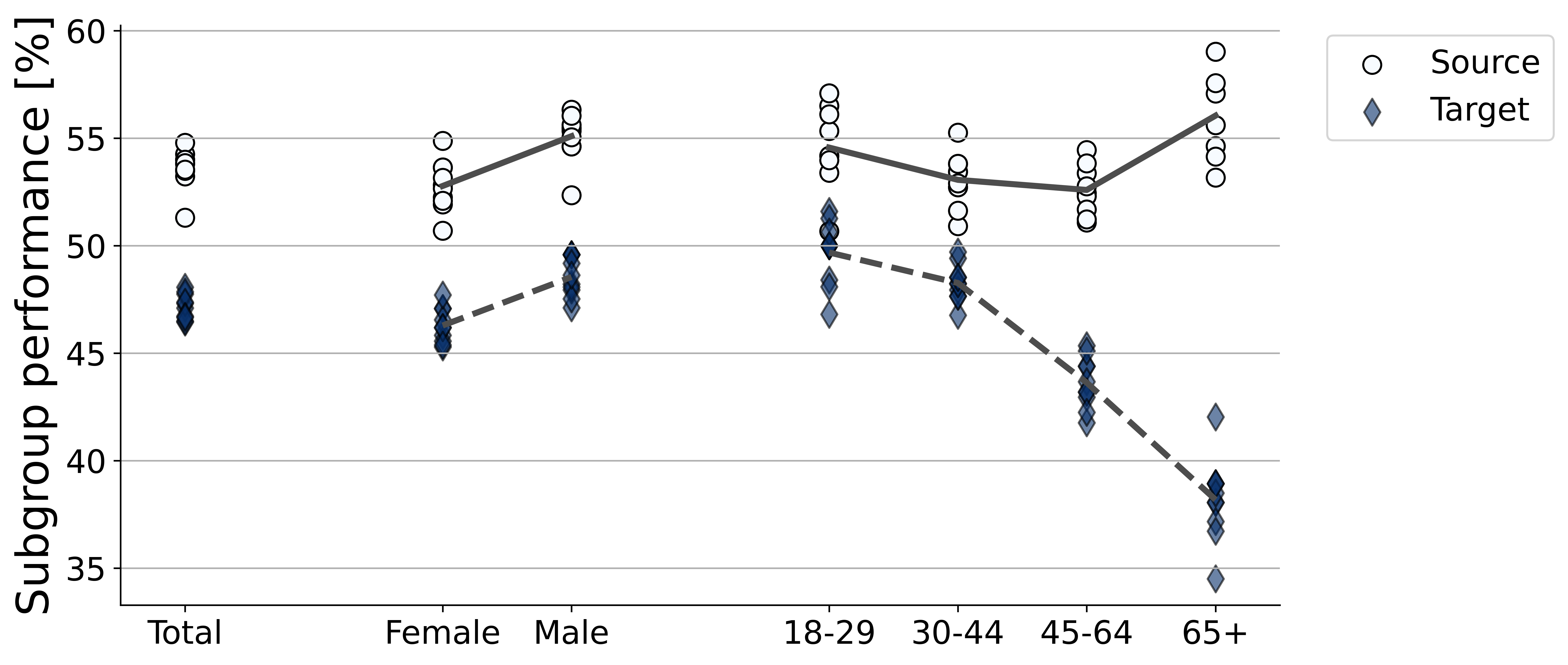
Figure 8: Model performance in dermatology, as estimated via Top-1 accuracy (in %). The plot displays the total performance, as well as performance stratified by sex and by age on the source (circles with plain line) and target (diamonds with dashed line) data. Each marker represents one replicate of the model.

E.2.3 Per condition model performance

We further compute model performance per condition when enough data samples are available both in the source and target data. We first observe that the tail of other conditions (‘other’, Figure 9(a)) shows more similarity with the source, and even improved performance. The fairness patterns for Melanocytic Nevus also seem to be similar across datasets, decreasing with age. On the other hand, SK/ISK shows an increase in performance with age in the target, but not in the source. This last result highlights that the changes in fairness patterns do not only result from changes in condition prevalence. We note that the analyses in this section include relatively low number of samples per subgroup.

(a)

(b)

(c)

Figure 9: Per condition model performance in dermatology, as estimated by top-3 accuracy (in %). (a) ’Other’. (b) Melanocytic Nevus. (c) SK/ISK.

E.2.4 Fitzpatrick’s skin type

In this target dataset, skin type is available as an attribute. We therefore perform similar analyses as performed for age and sex. We first observe that the proportions of cases across the different skin types are different across the source and target datasets (Figure 10(a), t-test: $p<0.001$).

(a)

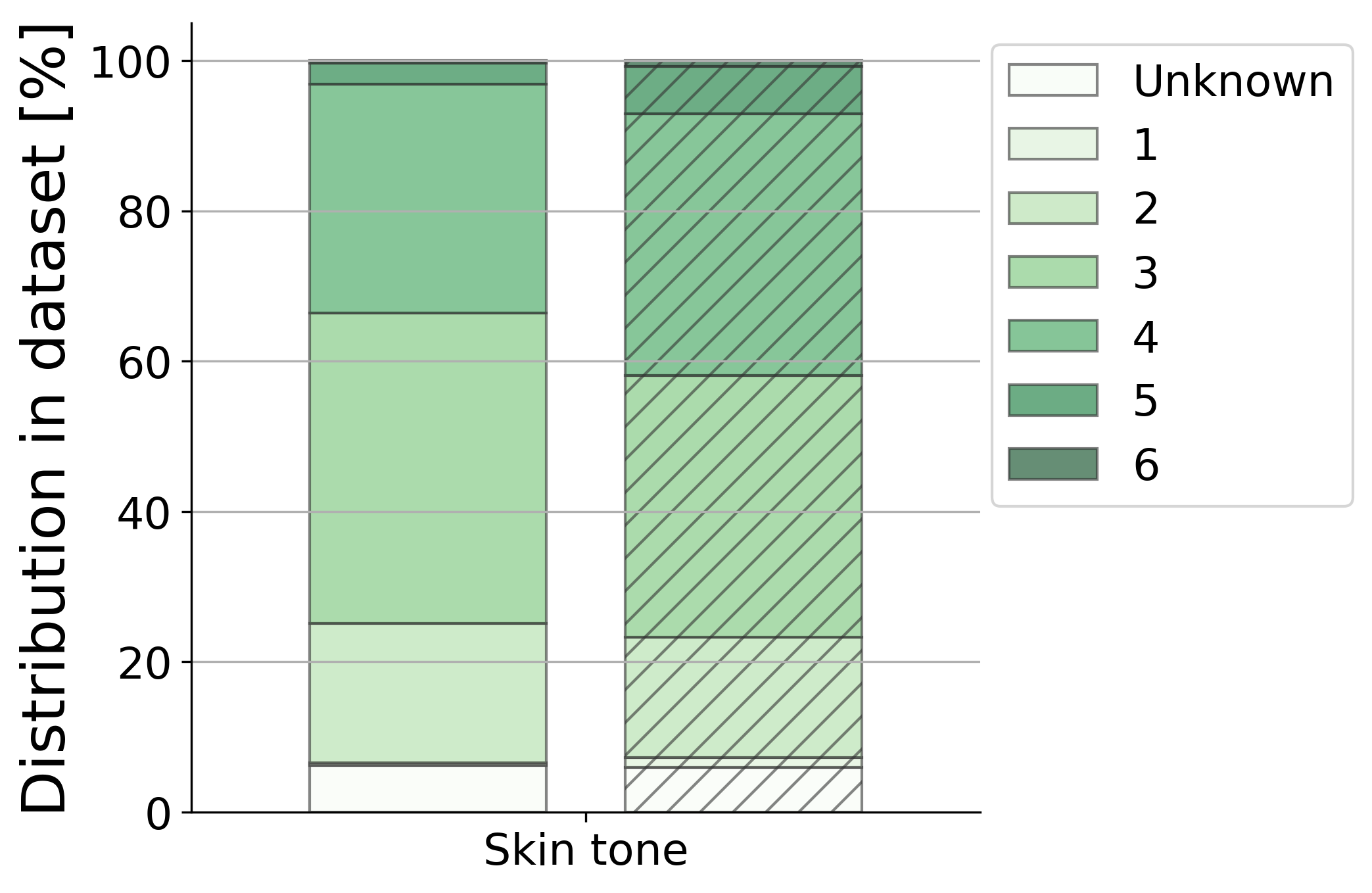
(b)

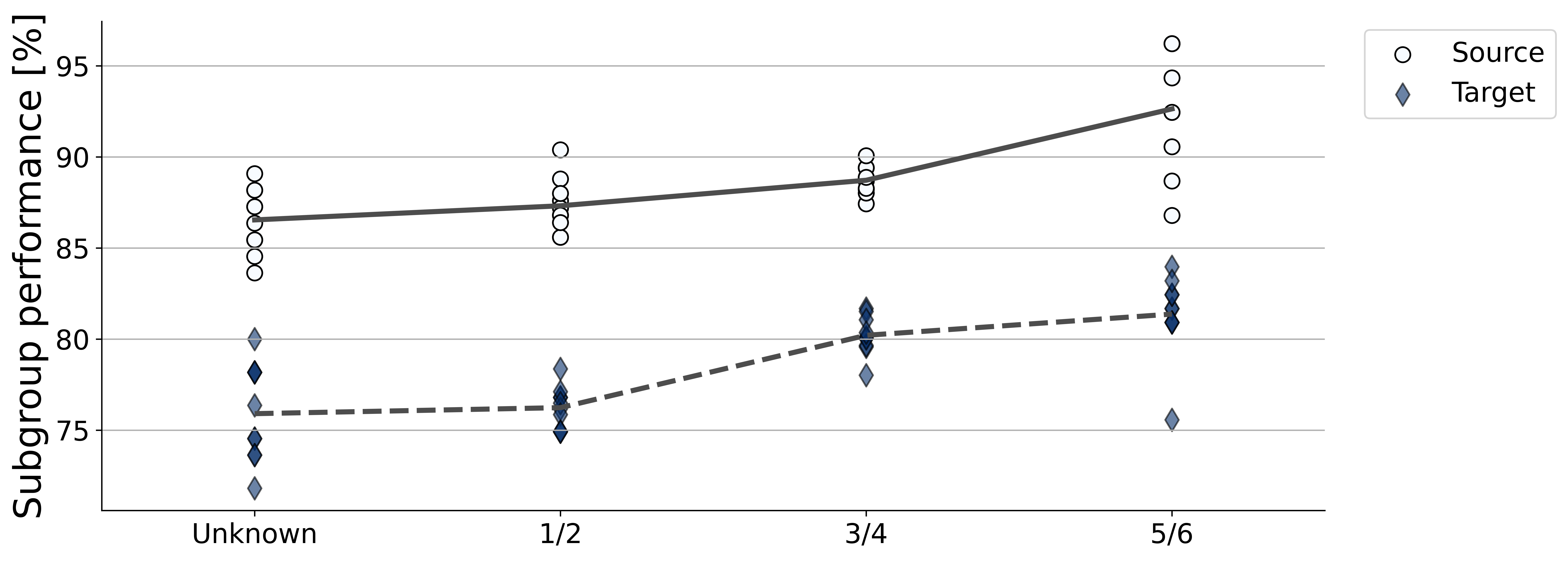
Figure 10: (a) Prevalence of the six Fitzpatrick’s skin types in each dataset (left: source, right: target). (b) Top-3 model performance for each subgroup in the source and in the target.

Due to a low number of examples for skin types 1 and 6 (in both datasets), we group skin types according to ‘unknown’, ‘1/2’, ‘3/4’ and ‘5/6’ before assessing top-3 performance per subgroup. We observe that model performance is relatively similar across the different subgroups, with the maximum pairwise difference being 6% on the source and 5.5% on the target (Figure 10(b)). We however note that, despite the groupings, the number of examples in group 5/6 remains low (source: $n=53$, target: $n=131$). Performance results in this group are hence to take with a grain of salt (as displayed by large variability across seeds), and single conditions cannot be investigated.

E.3 Second target dataset: skin cancer clinics in Australia

In this section, we repeat the analyses performed in the main text for another target dataset from skin cancer clinics in Australia and New Zealand that was partially labelled, leading to 21,661 cases used for model evaluation.

E.3.1 Fairness properties are affected by the environment

Detailed top-3 and top-1 model performance can be found in Tables 4 and 5, respectively. For top-1 accuracy, we observe similar results as for top-3 accuracy: model performance is relatively similar between groups on the source data, but differences become apparent on the target data (Figure 11).

Table 4: Top-3 model accuracy (in %) in the source and target data, on average across model runs.

Group	Source	Target
Total	$88.52\pm 0.68$	$70.87\pm 0.85$
Female	$88.95\pm 0.93$ (n=1,221)	$72.11\pm 0.98$ (n=10,195)
Male	$87.78\pm 0.52$ (n=703)	$69.77\pm 0.80$ (n=11,466)
$[18,30)$	$88.51\pm 1.11$ (n=563)	$87.52\pm 1.15$ (n=1,434)
$[30,45)$	$88.38\pm 1.02$ (n=548)	$77.64\pm 0.79$ (n=4,365)
$[45,65)$	$88.89\pm 0.70$ (n=619)	$68.39\pm 0.97$ (n=8,355)
$[65,90)$	$87.84\pm 1.70$ (n=194)	$66.20\pm 1.44$ (n=7,401)

Table 5: Top-1 model accuracy (in %) in the source and target data, on average across model runs.

Group	Source	Target
Total	$53.62\pm 0.88$	$32.14\pm 0.99$
Female	$53.62\pm 0.88$	$32.34\pm 1.14$
Male	$55.09\pm 1.05$	$31.96\pm 0.91$
$[18,30)$	$54.49\pm 1.73$	$45.80\pm 2.14$
$[30,45)$	$53.12\pm 1.14$	$36.63\pm 1.45$
$[45,65)$	$52.68\pm 0.92$	$29.32\pm 1.01$
$[65,90)$	$55.52\pm 2.00$	$29.72\pm 1.05$

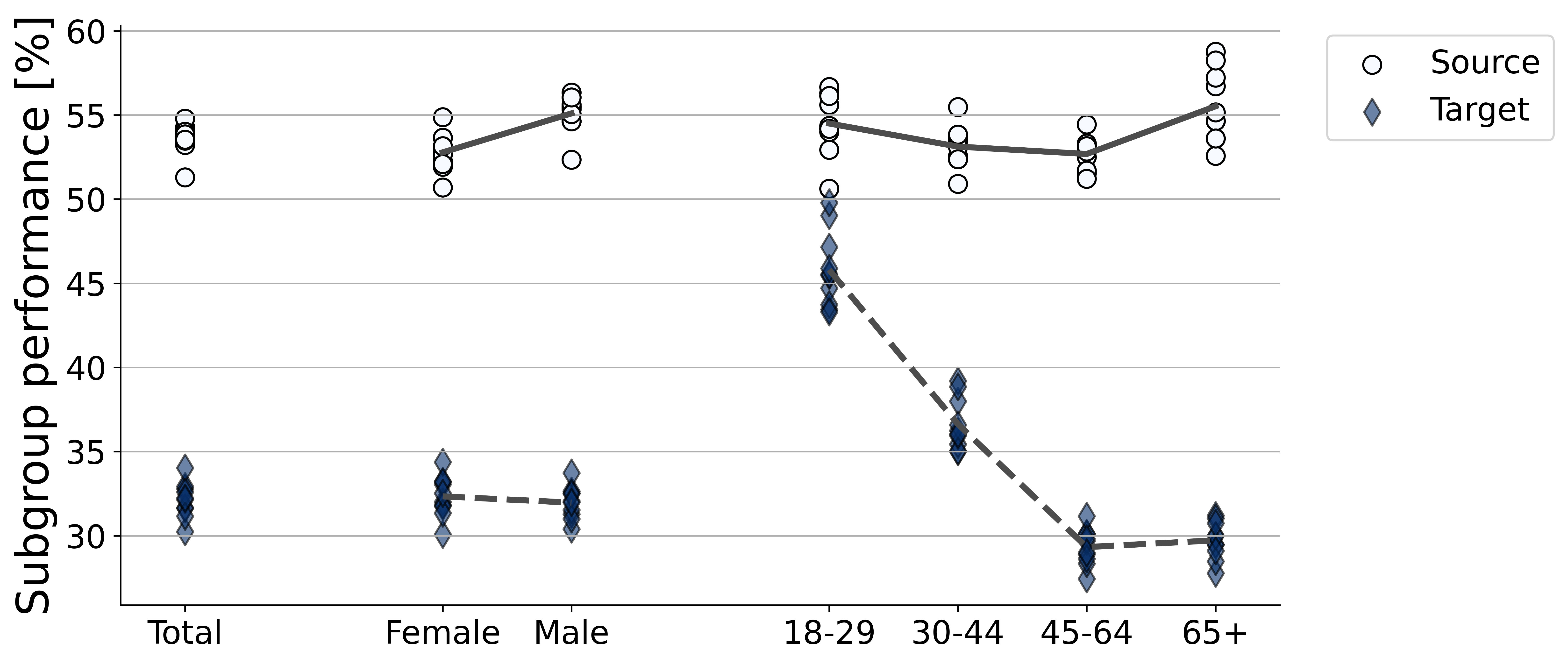
Figure 11: Model performance in dermatology, as estimated via Top-1 accuracy (in %). The plot displays the total performance, as well as performance stratified by sex and by age on the source (circles with plain line) and target (diamonds with dashed line) data. Each marker represents one replicate of the model.

E.3.2 Per condition model performance

We repeat the analyses for the same conditions depicted in Section E.2.3. We observe that the gaps between groups vary based on the condition, with the long tail of conditions (represented as a single ‘other’ condition in our task) being seemingly ‘fair’ on the source, but not on the target (Figure 12(a)). Some conditions like Melanocytic Nevus present disparities across age groups in both datasets (with the caveat of few test samples in the source data), with performance decreasing with increasing age (max gap in source: 24.47%, in target: 39.00%, Figure 12(b)). On the other hand, the SK/ISK condition displays similar performance across age groups in the source, but increasing performance with increasing age in the target (max gap in source: 4.00%, max gap in target: 31.78%, Figure 12(c)). Where the sample size allowed for comparisons, we therefore observe that the gaps across groups are not reproducible between the source and target data.

(a)

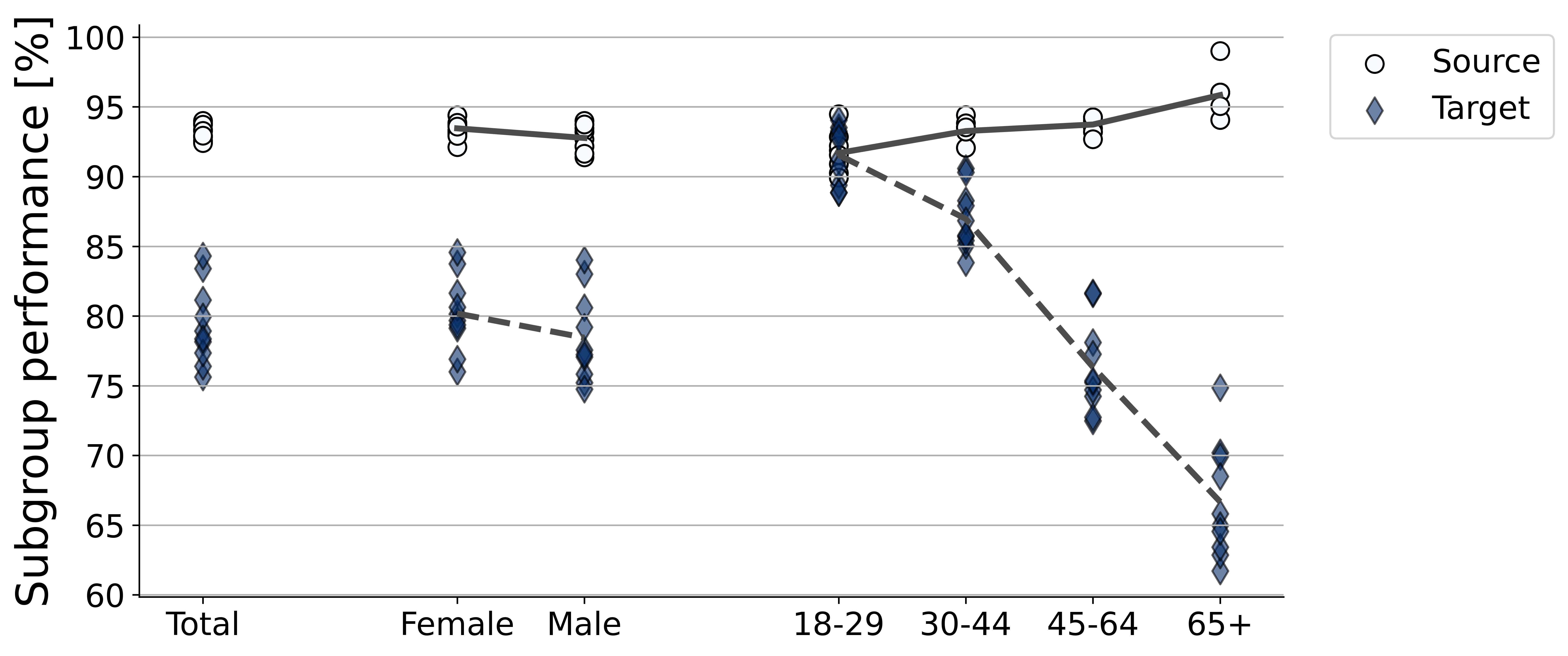
(b)

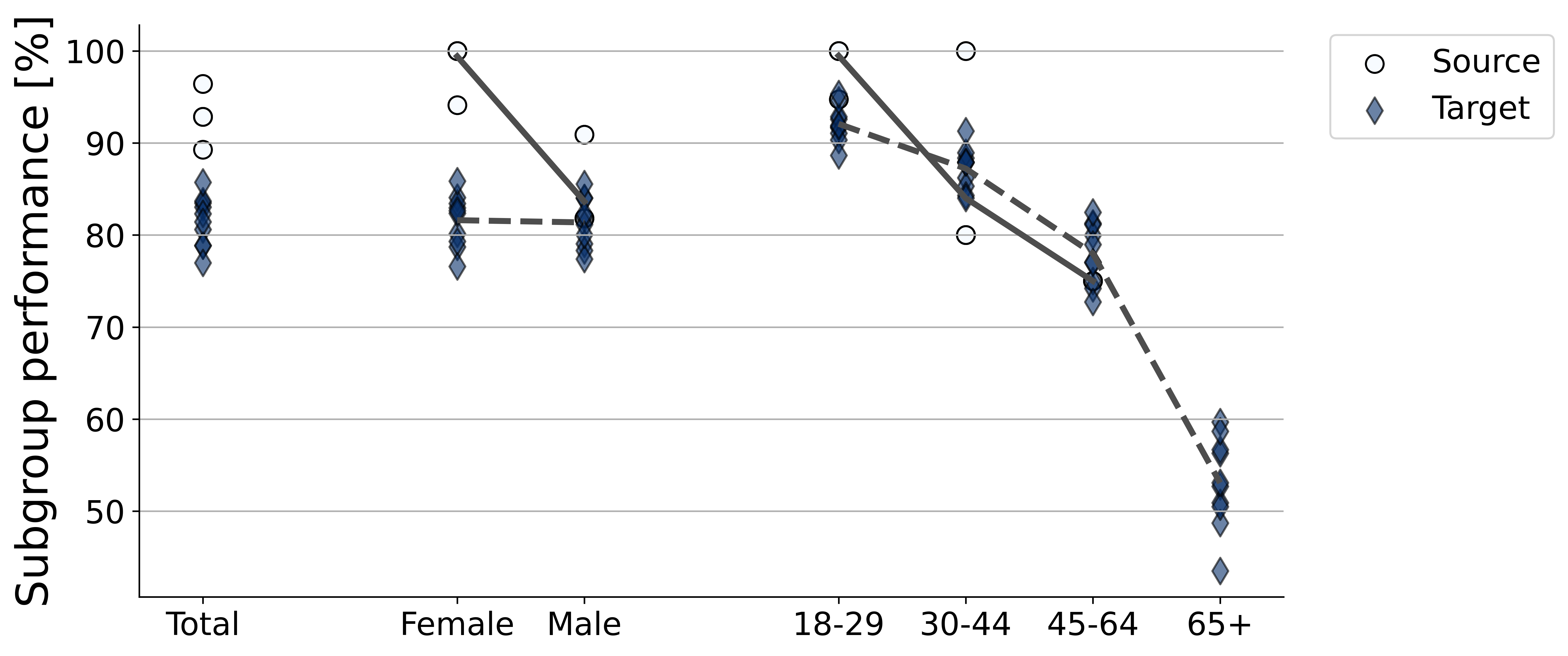
(c)

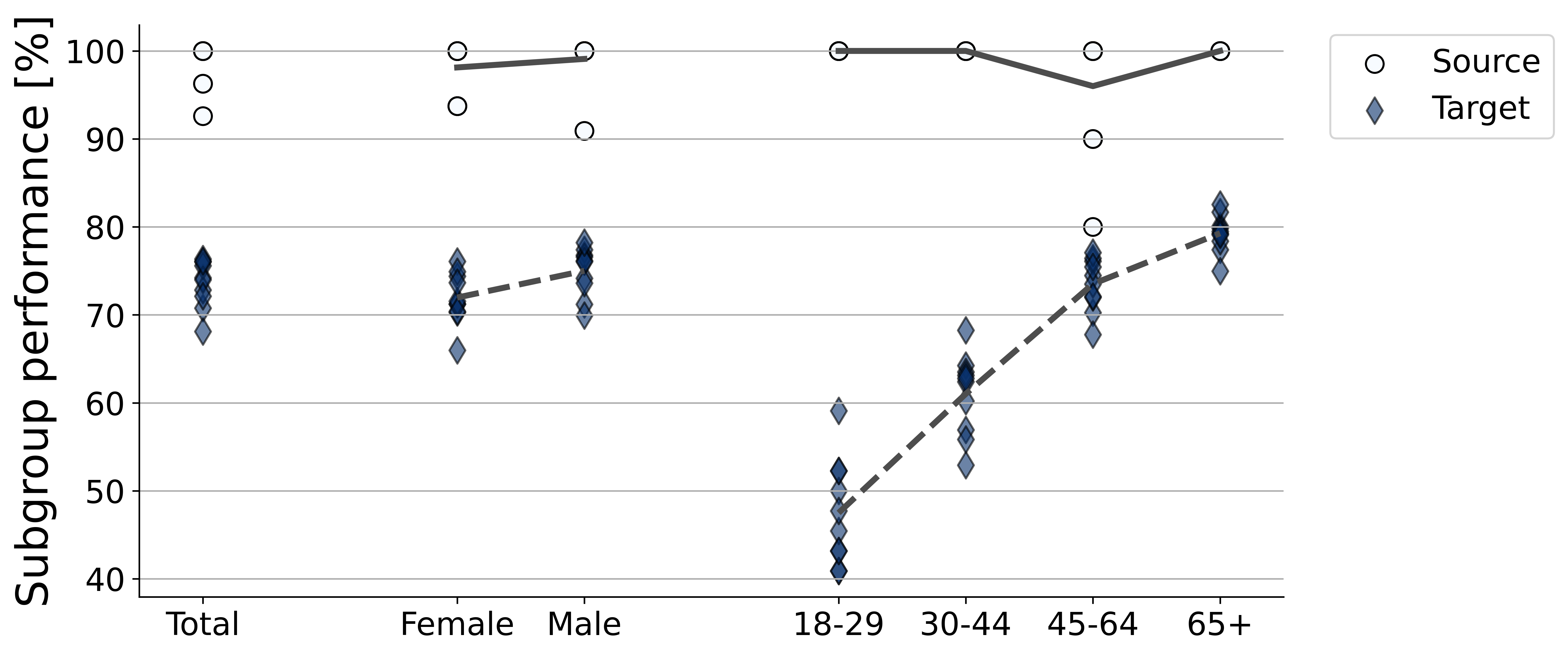
Figure 12: Per condition model performance in dermatology, as estimated by top-3 accuracy (in %). (a) ’Other’. (b) Melanocytic Nevus. (c) SK/ISK.

E.3.3 A compound shift

Referring to the same causal graph as in the main text, we apply our testing procedure to this second target set.

(a)

(b)

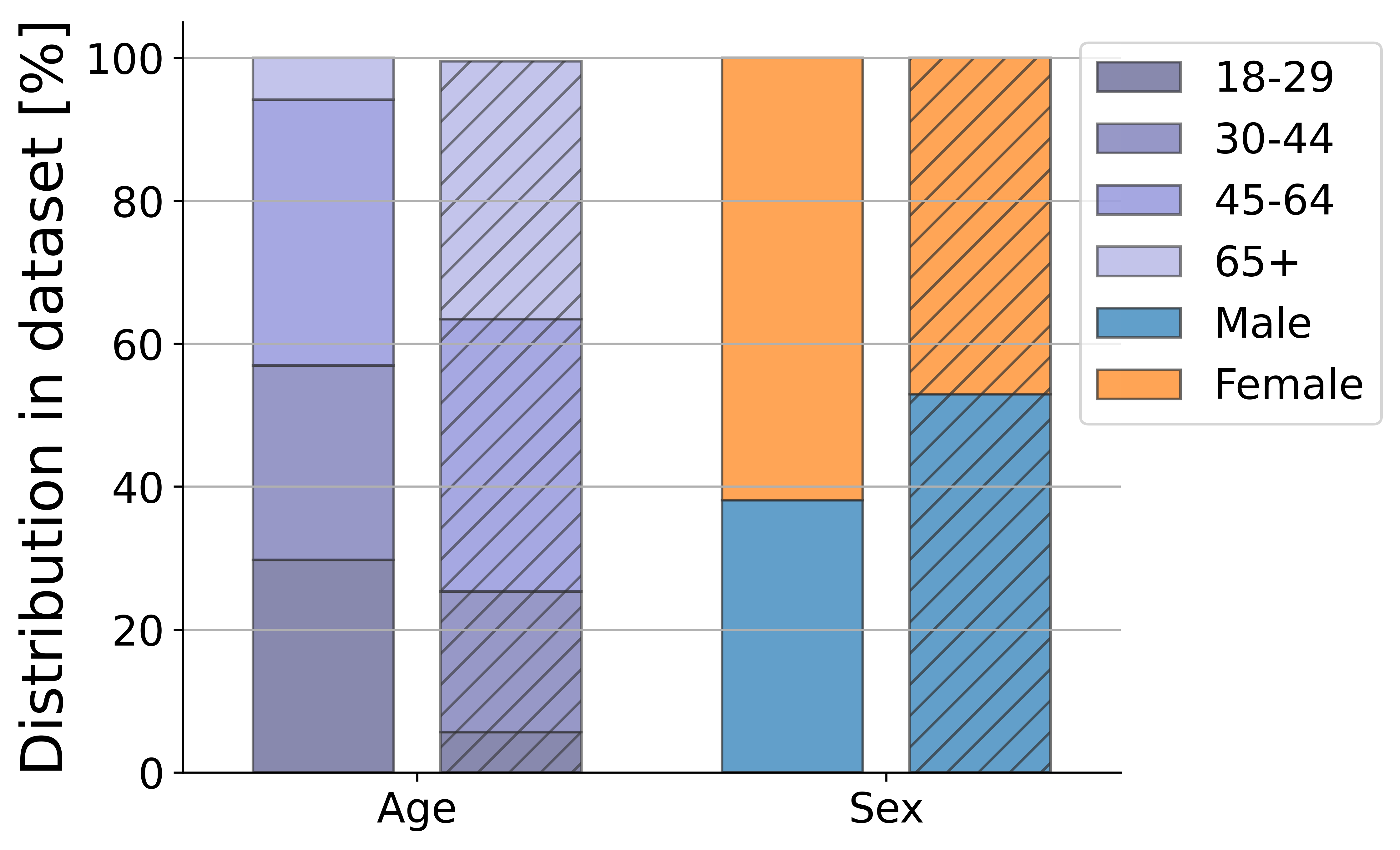
(c)

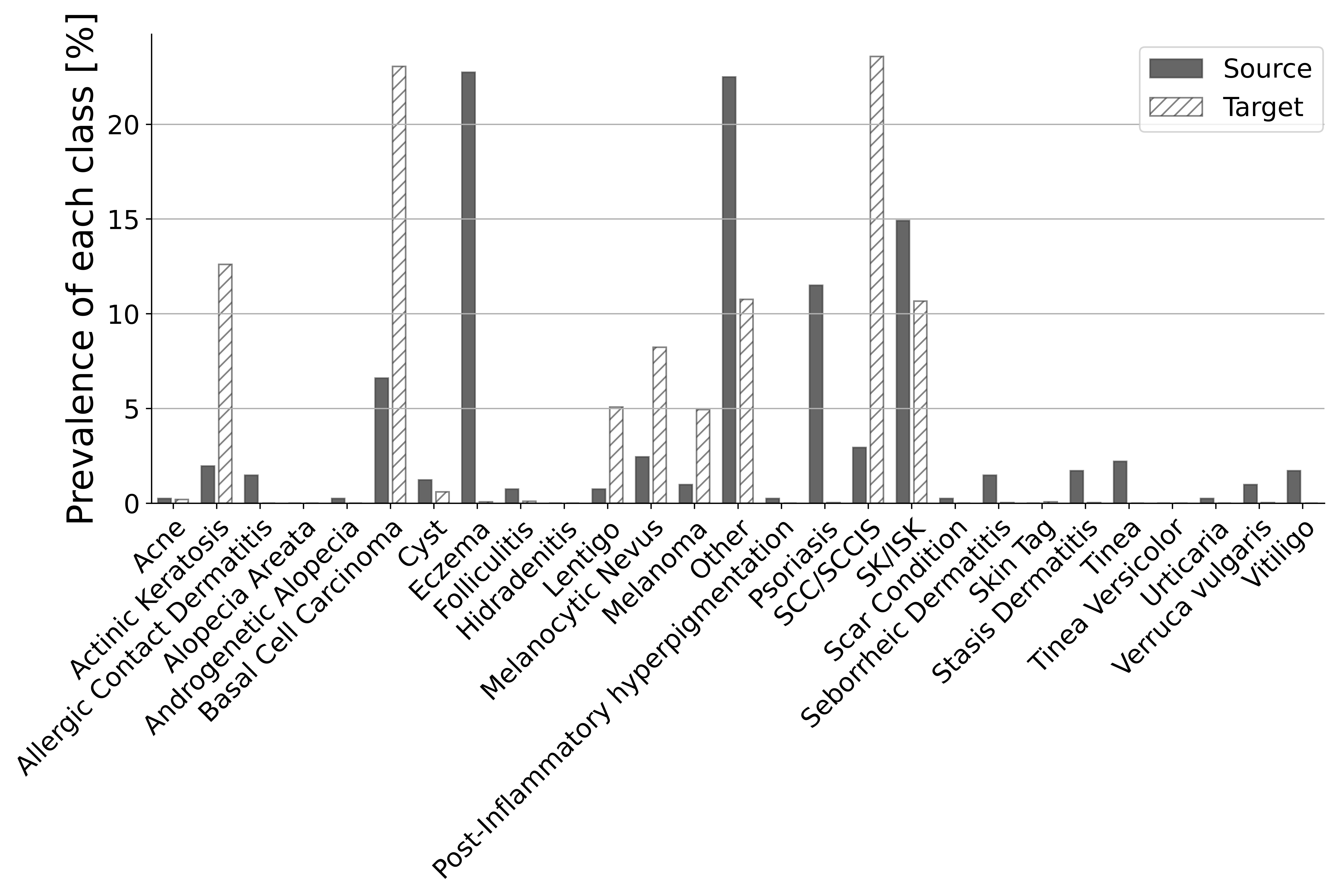
(d)

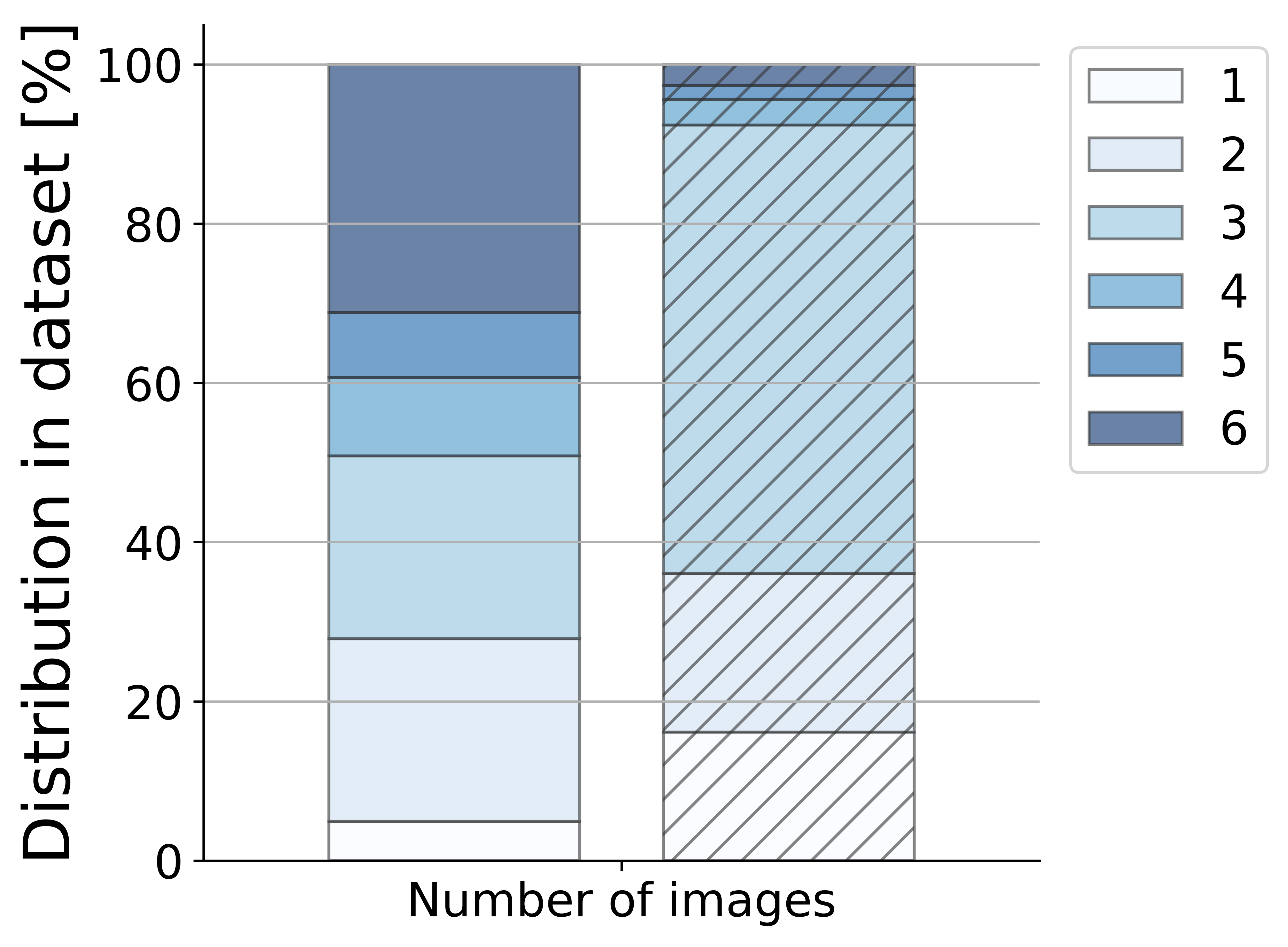
Figure 13: A compound shift in dermatology. (a) Simplified causal structure of the application. $A$ refers to demographic metadata, $Y$ to the skin condition as labelled by clinicians and $X$ represents the set of pictures of the skin pathology. In our setup, the environment $S$ directly affects all variables in the graph. (b) Distribution in the source train and in the target dataset of the sensitive attributes, computed in terms of percentage of pre-defined subgroups. (c) Prevalence of each condition in cases where the patients are female and over 65 years of age. (d) Distribution of the number of images in cases labelled as ‘SK/ISK’ in older females. The distributions in the source data are represented on the left, and their corresponding distributions in the target data on their immediate right with a hashed pattern.

Only age and sex are available in both datasets. These features have different distributions across the two datasets (see Fig. 13(b)), with the population in the source data being typically younger (median age: 40 years old, 25$\%$ quantile: 27, 75$\%$ quantile: 54) than in the target data (median age: 58 years old, 25$\%$ quantile: 44, 75$\%$ quantile: 70). The source distribution also includes more female patients than the target data (62$\%$, compared to 47$\%$). We therefore see direct effects of $S$ on $A$ (Fig. 13a, in purple).

We then assess whether $S$ directly affects the labels. Based on our testing procedure ($\{\mathbf{V}\}=\{A\}$), we obtain significant differences between $P(Y\,|\,A,S=0)$ and $P(Y\,|\,A,S=1)$ for 25 conditions ($p<0.05$, Bonferroni corrected). Fig.13(c) illustrates the label shift in a specific age and sex subgroup (here females aged 65+, 409 cases in the source, 3,198 in the target data). We see that the source data includes more cases of ‘eczema’ and ‘psoriasis’ and that cancerous conditions such as ‘basal cell carcinoma’ and ‘melanoma’ are more prevalent in the target data. Our results suggest that the environment also directly affects the labels (orange link in Fig.13(a)). We note that this analysis is limited to the distribution of labels and cannot assess differences in their quality: for instance, the labels for the source data were sourced from multiple clinicians, while some target labels were verified by biopsies. This is an added difference between the two environments (known as annotation shift, [7]) that only in-depth dataset knowledge can bring.

Finally, we consider whether the features of the images themselves (designated by $X$) are directly affected by $S$. Our weighted tests suggest a significant difference between these two distributions ($p<0.05$ on 21 dimensions, corrected). Fig.13(d) illustrates this difference by computing the number of images per case in the group of older females considered above with cases labelled as ‘SK/ISK’ ( source median: 3, $n=61$, target median: 2, $n=341$). This result suggests the existence of the direct path $S\rightarrow X$ and we add this relationship to the graph (green link in Fig.13(a)).

Based on these different analyses, we conclude that the environment is affecting all the variables in our simplified causal graph.

E.4 Joint training

In this section, we test whether joint training across datasets improves the transfer of fairness. We select the setup where the second target dataset (skin cancer clinics in Australia) is available for model development and add it to the source data, while we aim to obtain a robustly fair model on the first target dataset (teledermatology clinics in Colombia). This provides a training set that approximately doubles in size and now includes many more examples of cancer-related conditions.

We first assess whether the distributions of this joint source more closely match the distribution of the target. To this end, we perform the same statistical tests as previously but select half of the source data from each dataset. This simulates an equal proportion of each dataset in the joint distribution.

We observe that $A$, $Y|A$ (5 conditions with $p<0.05$ corrected) and $X|A,Y$ (2 conditions with $p<0.05$ corrected) display effects of the environment. Interestingly, the joint source introduces an effect of $S$ on different dimensions than previously. For instance, we now notice a difference in the distribution of cancer-related conditions between the joint source and the target that was not noticeable when comparing the original source (teledermatology clinics in the US) to the target.

In terms of model training, we observe that combining the two datasets for joint training is non-trivial. This is due to the datasets being very different (see section E.3). We take the simple approach of sampling a batch of each dataset with equal probability. This will oversample the data from the least represented dataset (here the original source). We note that this probability could be optimized over.

We report the results on the test set of the original source, on the test set of the joint source (randomly sampling $1,500$ cases from each dataset), and on the target set (Fig.14). We first observe that the overall performance gap between the source and the target has decreased. However, the fairness gap between source and target remains important, especially for age (max gap between groups: joint source = $4.33\%$, target = $11.4\%$).

a

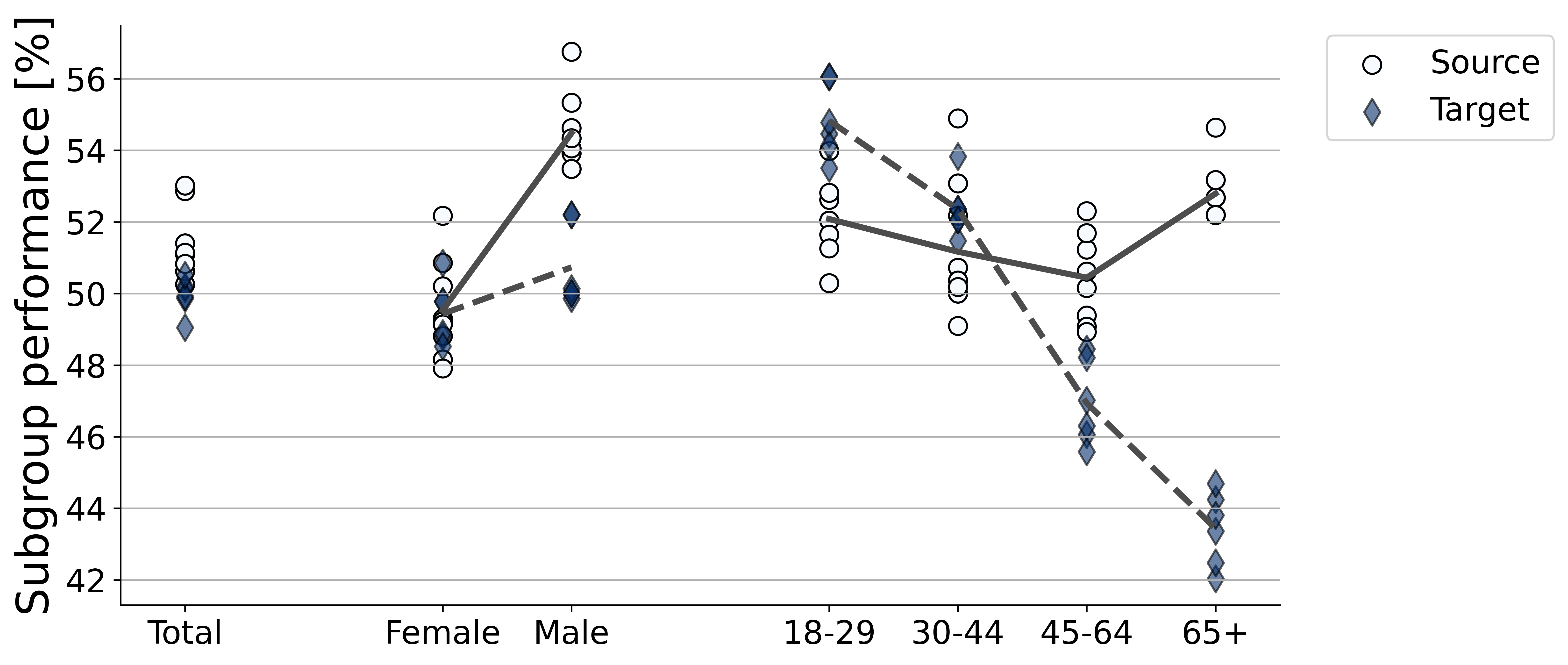
b

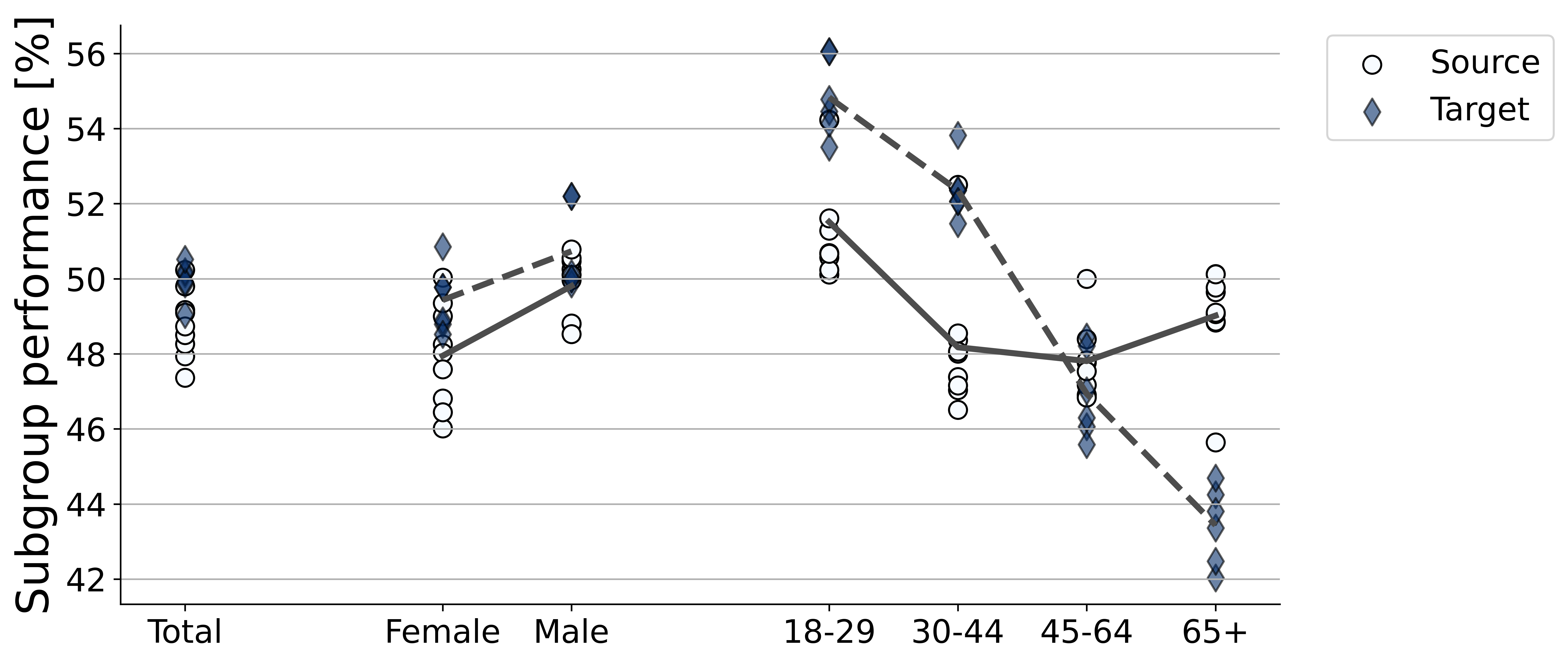
Figure 14: Model performance (top-1 accuracy) after joint training on the source data (circles) and target data (diamonds). (a) Original source test set. (b) Joint source test set.

We therefore conclude that joint training, as it does not introduce invariances to the environment here, does not guarantee an improvement in the transfer of fairness.

Appendix F Electronic health records

F.1 Dataset

Data availability: The de-identified EHR data is available based on a user agreement at Physionet [26].

Cohort selection: Our cohort includes patients with age $>$ 18 at time of admission and ICU length of stay (LOS) $>$ 1 day. We restrict the patient sequences to the first ICU admission, as in the MIMIC-Extract project [78], and additionally restrict to only those admissions with a FIRST_CAREUNIT defined in the MIMIC-III icustays table. This procedure results in a cohort of 28,083 patients.

Feature and target definition: The full feature set from [61] is used, leading to 31,303 binary features and 28,048 numeric features. The target is defined as a binary outcome, i.e. remaining ICU LOS $>$ 3 days, following the approach used in [78, 54].

Patient demographics are used as metadata for fairness mitigation and evaluation. For illustration, we focus on sex and age (bucketed as in the dermatology application).

Data splits: The FIRST_CAREUNIT defined in the MIMIC-III icustays table is used to split the dataset into a source dataset with 17,641 patients (MICU, SICU and TSICU) and target set with 10,442 patients (CCU, CSRU). The source dataset is then randomly split into training (80%), validation (5%), calibration (5%) and test (10%) sets.

F.2 Model and performance

As performed in [61, 72, 73], each patient’s medical history is converted to a time series of one-hour aggregates including the different structured data elements (medication, labs, vitals, …) represented by numerical and binary variables. Based on the first 24 hourly aggregates, we predict the binary label for prolonged length of stay using a recurrent network architecture [72, 73]. We then estimate model performance in terms of accuracy across patients and per sex and age subgroups. In addition to per-group metrics, we compute demographic parity and equalized odds.

Table 6 displays the detailed model performance on the source and on the target. On the source data, the model performs to $78.6\pm 0.7\%$ accuracy, with $\sim 1\%$ performance gap between sex groups and a gap of $7.4\%$ between age subgroups. Performance increases slightly between the two environments, with the model reaching $79.7\pm 0.9\%$. The gap between sexes increases to $2.7\%$ on the target data while it remains similar for age (7%). In terms of fairness metrics, demographic parity is $0.002\pm 0.002$ for sex on the source, and $0.016\pm 0.003$ on the target. It is $0.05\pm 0.006$ for age on the source, and $0.066\pm 0.010$ on the target. For both attributes, we hence observe an increase in demographic parity between the source and the target. Equalized odds do not display a significant difference between the two environments, for age or sex.

Table 6: Model accuracy (in %) in the source and target data, on average across model runs.

Group	Source	Target
Total	$78.6\pm 0.7$	$79.7\pm 0.9$
Female	$77.8\pm 0.8$	$78.0\pm 0.6$
Male	$79.2\pm 0.5$	$80.7\pm 0.5$
$[18,30)$	$84.0\pm 1.6$	$82.5\pm 0.9$
$[30,45)$	$82.8\pm 0.9$	$84.2\pm 0.9$
$[45,65)$	$78.8\pm 0.5$	$83.2\pm 0.6$
$[65,90)$	$76.6\pm 0.7$	$77.2\pm 0.6$

F.3 A compound shift

F.3.1 The ICU unit $S$ affects the comorbidities $M$

We define comorbidities according to [21, 74] using code in [31], obtaining a set of 30 comorbidities associated with each patient (multi-label). In this work, we refer to comorbidities as a ‘summary’ of ICD codes that represent the patient’s medical history prior to the current admission.

Statistical testing: We define IPW weights based on a logistic regression that predicts the environment based on 5,000 admissions from the source and 5,000 admissions from the target data. The classifier performs with an accuracy of 58.6% on a left-out test set comprising 20% of the data. For each comorbidity, we assess whether its prevalence is significantly affected by the environment using weighted tests. We observe that 5 comorbidities lead to significant results (after Bonferroni correction for multiple comparisons): pulmonary circulation, peripheral vascular, liver disease, metastatic cancer and solid tumor. We however caveat this analysis by the low number of patients whom have recorded comorbidities prior to admission, leading to many tests being invalid.

F.3.2 The ICU unit $S$ affects the treatments $T$

Definition of treatments: We identify treatments based on the ‘MedicationRequest’ field in the FHIR representation [57] of MIMIC. For each of those treatments, we construct a summary by counting the number of hourly requests in the first 24 hours after admission. This summary is used for illustrating specific medications (beta-blockers, vasopressors/inotropes and ACE inhibitors) and to control for treatments in section F.3.3. Given that this representation includes 5,873 dimensions, we build a further 1-dimensional summary [39] by training a model that predicts LOS from the time series of the medication requests on the source training split. This model reaches an accuracy of 76.9% (AUPRC: 0.54, AUROC: 0.75) on the source test split.

Statistical testing: We assess whether treatments are directly affected by $S$ by computing weights to balance $\{A,M\}$. We note that this analysis is limited as comorbidities are not reported for all patients. Nevertheless, a binary model discriminating between environments based on $\{A,M\}$ leads to 62% accuracy. Given the dimensionality of treatments, we perform a weighted test on the summary of treatments. Considering all medication, we observe that patients receive different treatments in different units (weighted test, $p=0.015$), hence $T\centernot{\mathrel{\perp\mspace{-10.0mu}\perp}}S|\{A,M\}$.

As an illustration, we estimate what proportion of patients receives treatments such as beta-blockers, vasopressors/inotropes and/or ACE inhibitors (Figure 15) for patients with (a) vascular comorbidities, and (b) tumor history.

a

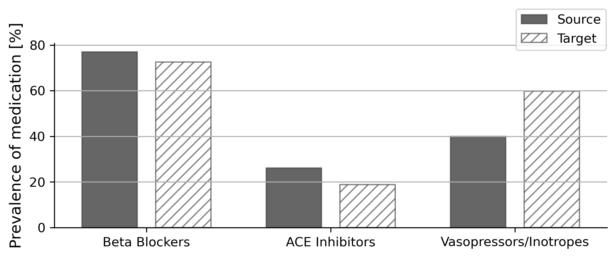
b

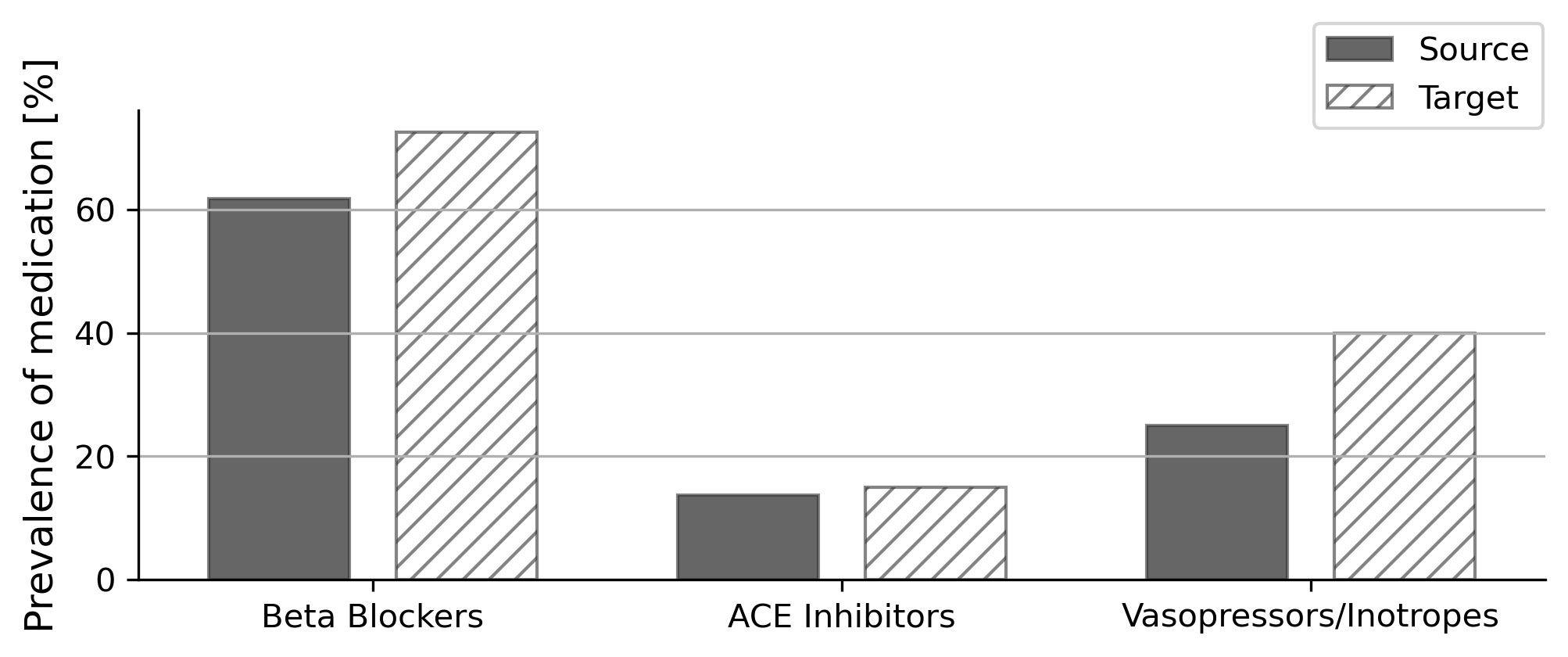
Figure 15: Per comorbity prevalence of treatment (in %). (a) Peripheral vascular comorbidities. (b) Solid tumor.

F.3.3 The ICU unit $S$ does not affect the length of stay $Y$

We refer to the summary of treatments of dimension 5,873 built above to define $T$ and build the feature set $\{A,M,T\}$ to estimate overlap weights such that we can test whether $P(Y|A,M,T,S=0)=P(Y|A,M,T,S=1)$. The treatment features with non-null values are normalized to be in the range [0, 1] before we build a classifier that distinguishes between the two environments. The model achieves $87.2\%$ accuracy in predicting the environment. We derive the weights for each data point in the two environments and assess with a weighted t-test whether the prevalence in the two environments is similar. Our results show that the ICU unit might not affect the prevalence of the length of stay ($p=0.18$). We however note that our analysis is limited by the large dimensionality of $\{A,M,T\}$ to build the weights. Indeed, the gradient boosted tree model $P(S|A,M,T)$ can then rely on many different signals to build its predictions [17] and display high variance across bootstraps. This would result in an under-powered test.

F.3.4 The ICU unit $S$ does not affect the labs and vitals $X$

Based on the causal graph, we use the same IPW weights as in Section F.3.3. We build a summary of $X$ by predicting $Y$ from all features that are not comorbidities, demographics or treatments. This recurrent model reaches 77.84% accuracy (AUPRC: 0.62, AUROC: 0.80) on the source test split. Based on this summary, we observe that labs and vitals do not display evidence of being affected by the environment ($p=0.45$).

References

- Adragna et al. [2020] Robert Adragna, Elliot Creager, David Madras, and Richard Zemel. Fairness and robustness in invariant learning: A case study in toxicity classification. November 2020.
- Agarwal et al. [2018] Alekh Agarwal, Alina Beygelzimer, Miroslav Dudik, John Langford, and Hanna Wallach. A reductions approach to fair classification. In Jennifer Dy and Andreas Krause, editors, Proceedings of the 35th International Conference on Machine Learning, volume 80 of Proceedings of Machine Learning Research, pages 60–69. PMLR, 10–15 Jul 2018. URL https://proceedings.mlr.press/v80/agarwal18a.html.
- Alabdulmohsin and Lučić [2021] Ibrahim Alabdulmohsin and Mario Lučić. A near-optimal algorithm for debiasing trained machine learning models. In 35th Conference on Neural Information Processing Systems, 2021. URL https://arxiv.org/abs/2106.12887.
- Arbour et al. [2021] David Arbour, Drew Dimmery, and Arjun Sondhi. Permutation weighting. 139:331–341, 2021.
- Barocas et al. [2019] Solon Barocas, Moritz Hardt, and Arvind Narayanan. Fairness and machine learning. fairmlbook.org, 2019.
- Ben-David et al. [2010] Shai Ben-David, John Blitzer, Koby Crammer, Alex Kulesza, Fernando Pereira, and Jennifer Wortman Vaughan. A theory of learning from different domains. Mach. Learn., 79(1):151–175, May 2010.
- Castro and Glocker [2020] Walker Ian Castro, Daniel C. and Ben Glocker. Causality matters in medical imaging. Nature Communications, 11, 2020.
- Chandola et al. [2009] Varun Chandola, Arindam Banerjee, and Vipin Kumar. Anomaly detection: A survey. ACM Comput. Surv., 41(3):1–58, July 2009.
- Charlson et al. [1987] M E Charlson, P Pompei, K L Ales, and C R MacKenzie. A new method of classifying prognostic comorbidity in longitudinal studies: development and validation. J. Chronic Dis., 40(5):373–383, 1987.
- Chen et al. [2021] Irene Y Chen, Emma Pierson, Sherri Rose, Shalmali Joshi, Kadija Ferryman, and Marzyeh Ghassemi. Ethical machine learning in healthcare. Annu Rev Biomed Data Sci, 4:123–144, July 2021.
- Cherepanova et al. [2021] Valeriia Cherepanova, Vedant Nanda, Micah Goldblum, John P Dickerson, and Tom Goldstein. Technical challenges for training fair neural networks. February 2021.
- Chiappa [2019] Silvia Chiappa. Path-Specific counterfactual fairness. AAAI, 33(01):7801–7808, July 2019.
- Coston et al. [2019] Amanda Coston, Karthikeyan Natesan Ramamurthy, Dennis Wei, Kush R. Varshney, Skyler Speakman, Zairah Mustahsan, and Supriyo Chakraborty. Fair transfer learning with missing protected attributes. In AAAI/ACM Conference on AI, Ethics, and Society, pages 91–98, 2019.
- Cowell et al. [2007] Robert G. Cowell, A. Philip Dawid, Steffen Lauritzen, and David J. Spiegelhalter. Probabilistic Networks and Expert Systems, Exact Computational Methods for Bayesian Networks. Springer-Verlag, 2007.
- Creager et al. [2020] Elliot Creager, David Madras, Toniann Pitassi, and Richard Zemel. Causal modeling for fairness in dynamical systems. 119:2185–2195, 2020.
- Creager et al. [2021] Elliot Creager, Joern-Henrik Jacobsen, and Richard Zemel. Environment inference for invariant learning. In Marina Meila and Tong Zhang, editors, Proceedings of the 38th International Conference on Machine Learning, volume 139 of Proceedings of Machine Learning Research, pages 2189–2200. PMLR, 2021.
- D’Amour et al. [2020] Alexander D’Amour, Katherine Heller, Dan Moldovan, Ben Adlam, Babak Alipanahi, Alex Beutel, Christina Chen, Jonathan Deaton, Jacob Eisenstein, Matthew D Hoffman, Farhad Hormozdiari, Neil Houlsby, Shaobo Hou, Ghassen Jerfel, Alan Karthikesalingam, Mario Lucic, Yian Ma, Cory McLean, Diana Mincu, Akinori Mitani, Andrea Montanari, Zachary Nado, Vivek Natarajan, Christopher Nielson, Thomas F Osborne, Rajiv Raman, Kim Ramasamy, Rory Sayres, Jessica Schrouff, Martin Seneviratne, Shannon Sequeira, Harini Suresh, Victor Veitch, Max Vladymyrov, Xuezhi Wang, Kellie Webster, Steve Yadlowsky, Taedong Yun, Xiaohua Zhai, and D Sculley. Underspecification presents challenges for credibility in modern machine learning. November 2020.
- Deyo et al. [1992] R A Deyo, D C Cherkin, and M A Ciol. Adapting a clinical comorbidity index for use with ICD-9-CM administrative databases. J. Clin. Epidemiol., 45(6):613–619, June 1992.
- Du and Wu [2021] Wei Du and Xintao Wu. Fair and robust classification under sample selection bias. In ACM International Conference on Information & Knowledge Management, pages 2999–3003, 2021.
- Dwork et al. [2012] Cynthia Dwork, Moritz Hardt, Toniann Pitassi, Omer Reingold, and Richard Zemel. Fairness through awareness. In Innovations in Theoretical Computer Science, 2012.
- Elixhauser et al. [1998] A Elixhauser, C Steiner, D R Harris, and R M Coffey. Comorbidity measures for use with administrative data. Med. Care, 36(1):8–27, January 1998.
- Farahani et al. [2020] Abolfazl Farahani, Sahar Voghoei, Khaled Rasheed, and Hamid R Arabnia. A brief review of domain adaptation. October 2020.
- Finkelstein et al. [2021] Noam Finkelstein, Roy Adams, Suchi Saria, and Ilya Shpitser. Partial identifiability in discrete data with measurement error. In Proceedings of 37th Conference on Uncertainty in Artificial Intelligence, July 2021.
- Finlayson et al. [2021] Samuel G Finlayson, Adarsh Subbaswamy, Karandeep Singh, John Bowers, Annabel Kupke, Jonathan Zittrain, Isaac S Kohane, and Suchi Saria. The clinician and dataset shift in artificial intelligence. N. Engl. J. Med., 385(3):283–286, July 2021.
- Garg et al. [2020] Saurabh Garg, Yifan Wu, Sivaraman Balakrishnan, and Zachary Lipton. A unified view of label shift estimation. In H Larochelle, M Ranzato, R Hadsell, M F Balcan, and H Lin, editors, Advances in Neural Information Processing Systems, volume 33, pages 3290–3300. Curran Associates, Inc., 2020.
- Goldberger et al. [2000] A L Goldberger, L A Amaral, L Glass, J M Hausdorff, P C Ivanov, R G Mark, J E Mietus, G B Moody, C K Peng, and H E Stanley. PhysioBank, PhysioToolkit, and PhysioNet: components of a new research resource for complex physiologic signals. Circulation, 101(23):E215–20, June 2000.
- Gretton et al. [2012] Arthur Gretton, Karsten M Borgwardt, Malte J Rasch, and Bernhard Scholkopf. A kernel Two-Sample test. J. Mach. Learn. Res., 13(25):723–773, 2012.
- Halfon et al. [2002] Patricia Halfon, Yves Eggli, Guy van Melle, Julia Chevalier, Jean Blaise Wasserfallen, and Bernard Burnand. Measuring potentially avoidable hospital readmissions. J. Clin. Epidemiol., 55(6):573–587, June 2002.
- Imai and van Dyk [2004] Kosuke Imai and David A van Dyk. Causal inference with general treatment regimes. J. Am. Stat. Assoc., 99(467):854–866, September 2004.
- Johnson et al. [2016] Alistair E W Johnson, Tom J Pollard, Lu Shen, Li-Wei H Lehman, Mengling Feng, Mohammad Ghassemi, Benjamin Moody, Peter Szolovits, Leo Anthony Celi, and Roger G Mark. MIMIC-III, a freely accessible critical care database. Sci Data, 3:160035, May 2016.
- Johnson et al. [2018] Alistair Ew Johnson, David J Stone, Leo A Celi, and Tom J Pollard. The MIMIC code repository: enabling reproducibility in critical care research. J. Am. Med. Inform. Assoc., 25(1):32–39, January 2018.
- Kallus and Zhou [2018] Nathan Kallus and Angela Zhou. Residual unfairness in fair machine learning from prejudiced data. In International Conference on Machine Learning, pages 2439–2448, 2018.
- Koh et al. [2020] Pang Wei Koh, Shiori Sagawa, Henrik Marklund, Sang Michael Xie, Marvin Zhang, Akshay Balsubramani, Weihua Hu, Michihiro Yasunaga, Richard Lanas Phillips, Irena Gao, Tony Lee, Etienne David, Ian Stavness, Wei Guo, Berton A Earnshaw, Imran S Haque, Sara Beery, Jure Leskovec, Anshul Kundaje, Emma Pierson, Sergey Levine, Chelsea Finn, and Percy Liang. WILDS: A benchmark of in-the-wild distribution shifts. December 2020.
- Kolesnikov et al. [2020] Alexander Kolesnikov, Lucas Beyer, Xiaohua Zhai, Joan Puigcerver, Jessica Yung, Sylvain Gelly, and Neil Houlsby. Big transfer (BiT): General visual representation learning. In ECCV, 2020.
- Koller and Friedman [2009] Daphne Koller and Nir Friedman. Probabilistic Graphical Models: Principles and Techniques. MIT Press, 2009.
- Lan and Huan [2017] Chao Lan and Jun Huan. Discriminatory transfer. July 2017.
- Li et al. [2008] Bing Li, Dewey Evans, Peter Faris, Stafford Dean, and Hude Quan. Risk adjustment performance of charlson and elixhauser comorbidities in ICD-9 and ICD-10 administrative databases. BMC Health Serv. Res., 8:12, January 2008.
- Li et al. [2019] Fan Li, Laine E Thomas, and Fan Li. Addressing extreme propensity scores via the overlap weights. Am. J. Epidemiol., 188(1):250–257, January 2019.
- Lipton et al. [2018] Zachary Lipton, Yu-Xiang Wang, and Alexander Smola. Detecting and correcting for label shift with black box predictors. In Jennifer Dy and Andreas Krause, editors, Proceedings of the 35th International Conference on Machine Learning, volume 80 of Proceedings of Machine Learning Research, pages 3122–3130. PMLR, 2018.
- Liu et al. [2020] Yuan Liu, Ayush Jain, Clara Eng, David H Way, Kang Lee, Peggy Bui, Kimberly Kanada, Guilherme de Oliveira Marinho, Jessica Gallegos, Sara Gabriele, Vishakha Gupta, Nalini Singh, Vivek Natarajan, Rainer Hofmann-Wellenhof, Greg S Corrado, Lily H Peng, Dale R Webster, Dennis Ai, Susan J Huang, Yun Liu, R Carter Dunn, and David Coz. A deep learning system for differential diagnosis of skin diseases. Nat. Med., 26(6):900–908, June 2020.
- Magliacane et al. [2018] Sara Magliacane, Thijs van Ommen, Tom Claassen, Stephan Bongers, Philip Versteeg, and Joris M Mooij. Domain adaptation by using causal inference to predict invariant conditional distributions. In S Bengio, H Wallach, H Larochelle, K Grauman, N Cesa-Bianchi, and R Garnett, editors, Advances in Neural Information Processing Systems, volume 31. Curran Associates, Inc., 2018.
- Markou and Singh [2003] Markos Markou and Sameer Singh. Novelty detection: a review—part 1: statistical approaches. Signal Processing, 83(12):2481–2497, December 2003.
- Mehrabi et al. [2019] Ninareh Mehrabi, Fred Morstatter, Nripsuta Saxena, Kristina Lerman, and Aram Galstyan. A survey on bias and fairness in machine learning. arXiv preprint arXiv:1908.09635, 2019.
- Mhasawade et al. [2020] Vishwali Mhasawade, Nabeel Abdur Rehman, and Rumi Chunara. Population-aware hierarchical bayesian domain adaptation via multi-component invariant learning. In Proceedings of the ACM Conference on Health, Inference, and Learning, CHIL ’20, pages 182–192, New York, NY, USA, April 2020. Association for Computing Machinery.
- Mooij et al. [2020] Joris M Mooij, Sara Magliacane, and Tom Claassen. Joint causal inference from multiple contexts. J. Mach. Learn. Res., 21(99):1–108, 2020.
- Nanda et al. [2021] Vedant Nanda, Samuel Dooley, Sahil Singla, Soheil Feizi, and John P Dickerson. Fairness through robustness: Investigating robustness disparity in deep learning. In Proceedings of the 2021 ACM Conference on Fairness, Accountability, and Transparency, FAccT ’21, pages 466–477, New York, NY, USA, March 2021. Association for Computing Machinery.
- Nestor et al. [2019] Bret Nestor, Matthew B A McDermott, Willie Boag, Gabriela Berner, Tristan Naumann, Michael C Hughes, Anna Goldenberg, and Marzyeh Ghassemi. Feature robustness in non-stationary health records: Caveats to deployable model performance in common clinical machine learning tasks. In Finale Doshi-Velez, Jim Fackler, Ken Jung, David Kale, Rajesh Ranganath, Byron Wallace, and Jenna Wiens, editors, Proceedings of the 4th Machine Learning for Healthcare Conference, volume 106 of Proceedings of Machine Learning Research, pages 381–405, Ann Arbor, Michigan, 2019. PMLR.
- Oneto and Chiappa [2020] Luca Oneto and Silvia Chiappa. Fairness in machine learning. In L. Oneto, N. Navarin, A. Sperduti, and D. Anguita, editors, Recent Trends in Learning From Data. Studies in Computational Intelligence, volume 896. Springer, Cham, 2020.
- Oneto et al. [2019] Luca Oneto, Michele Donini, A. Maurer, and Massimiliano Pontil. Learning fair and transferable representations, 2019.
- Pan and Yang [2010] Sinno Jialin Pan and Qiang Yang. A survey on transfer learning. IEEE Trans. Knowl. Data Eng., 22(10):1345–1359, October 2010.
- Pearl [1988] Judea Pearl. Probabilistic Reasoning in Intelligent Systems: Networks of Plausible Inference. Morgan Kaufmann Publishers Inc., 1988.
- Pearl [2000] Judea Pearl. Causality: Models, Reasoning, and Inference. Cambridge University Press, 2000.
- Pedregosa et al. [2011] F. Pedregosa, G. Varoquaux, A. Gramfort, V. Michel, B. Thirion, O. Grisel, M. Blondel, P. Prettenhofer, R. Weiss, V. Dubourg, J. Vanderplas, A. Passos, D. Cournapeau, M. Brucher, M. Perrot, and E. Duchesnay. Scikit-learn: Machine learning in Python. Journal of Machine Learning Research, 12:2825–2830, 2011.
- Pfohl et al. [2021] Stephen R Pfohl, Agata Foryciarz, and Nigam H Shah. An empirical characterization of fair machine learning for clinical risk prediction. J. Biomed. Inform., 113:103621, January 2021.
- Pierpont and Parenti [1999] G L Pierpont and C M Parenti. Physician risk assessment and APACHE scores in cardiac care units. Clin. Cardiol., 22(5):366–368, May 1999.
- Rabanser et al. [2019] Stephan Rabanser, Stephan Günnemann, and Zachary C Lipton. Failing loudly: An empirical study of methods for detecting dataset shift. In 33rd Conference on Neural Information Processing Systems, 2019.
- Rajkomar et al. [2018] Alvin Rajkomar, Eyal Oren, Kai Chen, Andrew M Dai, Nissan Hajaj, Michaela Hardt, Peter J Liu, Xiaobing Liu, Jake Marcus, Mimi Sun, Patrik Sundberg, Hector Yee, Kun Zhang, Yi Zhang, Gerardo Flores, Gavin E Duggan, Jamie Irvine, Quoc Le, Kurt Litsch, Alexander Mossin, Justin Tansuwan, De Wang, James Wexler, Jimbo Wilson, Dana Ludwig, Samuel L Volchenboum, Katherine Chou, Michael Pearson, Srinivasan Madabushi, Nigam H Shah, Atul J Butte, Michael D Howell, Claire Cui, Greg S Corrado, and Jeffrey Dean. Scalable and accurate deep learning with electronic health records. NPJ Digit Med, 1:18, May 2018.
- Rosenbaum and Rubin [1983] Paul R Rosenbaum and Donald B Rubin. The central role of the propensity score in observational studies for causal effects. Biometrika, 70(1):41–55, April 1983.
- Ross et al. [2017] Andrew Slavin Ross, Michael C Hughes, and Finale Doshi-Velez. Right for the right reasons: Training differentiable models by constraining their explanations. In Proceedings of the Twenty-Sixth International Joint Conference on Artificial Intelligence, pages 2662–2670, California, August 2017. International Joint Conferences on Artificial Intelligence Organization.
- Roy et al. [2021a] Abhijit Guha Roy, Jie Ren, Shekoofeh Azizi, Aaron Loh, Vivek Natarajan, Basil Mustafa, Nick Pawlowski, Jan Freyberg, Yuan Liu, Zach Beaver, Nam Vo, Peggy Bui, Samantha Winter, Patricia MacWilliams, Greg S Corrado, Umesh Telang, Yun Liu, Taylan Cemgil, Alan Karthikesalingam, Balaji Lakshminarayanan, and Jim Winkens. Does your dermatology classifier know what it doesn’t know? detecting the Long-Tail of unseen conditions. April 2021a.
- Roy et al. [2021b] Subhrajit Roy, Diana Mincu, Eric Loreaux, Anne Mottram, Ivan Protsyuk, Natalie Harris, Yuan Xue, Jessica Schrouff, Hugh Montgomery, Alistair Connell, Nenad Tomasev, Alan Karthikesalingam, and Martin Seneviratne. Multitask prediction of organ dysfunction in the intensive care unit using sequential subnetwork routing. J. Am. Med. Inform. Assoc., June 2021b.
- Sambasivan et al. [2021] Nithya Sambasivan, Erin Arnesen, Ben Hutchinson, Tulsee Doshi, and Vinodkumar Prabhakaran. Re-imagining algorithmic fairness in india and beyond. January 2021.
- Schölkopf et al. [2012] Bernhard Schölkopf, Dominik Janzing, Jonas Peters, Eleni Sgouritsa, Kun Zhang, and Joris Mooij. On causal and anticausal learning. In International Conference on Machine Learning, pages 459–466, 2012.
- Schumann et al. [2019] Candice Schumann, Xuezhi Wang, Alex Beutel, Jilin Chen, Hai Qian, and Ed H Chi. Transfer of machine learning fairness across domains. June 2019.
- Shimodaira [2000] Hidetoshi Shimodaira. Improving predictive inference under covariate shift by weighting the log-likelihood function. Journal of statistical planning and inference, 90(2):227–244, 2000.
- Simpson et al. [2019] Becks Simpson, Francis Dutil, Yoshua Bengio, and Joseph Paul Cohen. GradMask: Reduce overfitting by regularizing saliency. April 2019.
- Singh et al. [2021] Harvineet Singh, Rina Singh, Vishwali Mhasawade, and Rumi Chunara. Fairness violations and mitigation under covariate shift. In Proceedings of the 2021 ACM Conference on Fairness, Accountability, and Transparency, pages 3–13. Association for Computing Machinery, New York, NY, USA, March 2021.
- Singh et al. [2022] Harvineet Singh, Vishwali Mhasawade, and Rumi Chunara. Generalizability challenges of mortality risk prediction models: A retrospective analysis on a multi-center database. PLOS Digital Health, 1(4):e0000023, April 2022.
- Slack et al. [2020] Dylan Slack, Sorelle A Friedler, and Emile Givental. Fairness warnings and fair-MAML: learning fairly with minimal data. In Proceedings of the 2020 Conference on Fairness, Accountability, and Transparency, FAT* ’20, pages 200–209, New York, NY, USA, January 2020. Association for Computing Machinery.
- Subbaswamy et al. [2020] Adarsh Subbaswamy, Roy Adams, and Suchi Saria. Evaluating model robustness and stability to dataset shift. October 2020.
- Taskesen et al. [2020] Bahar Taskesen, Viet Anh Nguyen, Daniel Kuhn, and José H. Blanchet. A distributionally robust approach to fair classification, 2020.
- Tomašev et al. [2019] Nenad Tomašev, Xavier Glorot, Jack W Rae, Michal Zielinski, Harry Askham, Andre Saraiva, Anne Mottram, Clemens Meyer, Suman Ravuri, Ivan Protsyuk, Alistair Connell, Cían O Hughes, Alan Karthikesalingam, Julien Cornebise, Hugh Montgomery, Geraint Rees, Chris Laing, Clifton R Baker, Kelly Peterson, Ruth Reeves, Demis Hassabis, Dominic King, Mustafa Suleyman, Trevor Back, Christopher Nielson, Joseph R Ledsam, and Shakir Mohamed. A clinically applicable approach to continuous prediction of future acute kidney injury. Nature, 572(7767):116–119, August 2019.
- Tomašev et al. [2021] Nenad Tomašev, Natalie Harris, Sebastien Baur, Anne Mottram, Xavier Glorot, Jack W Rae, Michal Zielinski, Harry Askham, Andre Saraiva, Valerio Magliulo, Clemens Meyer, Suman Ravuri, Ivan Protsyuk, Alistair Connell, Cían O Hughes, Alan Karthikesalingam, Julien Cornebise, Hugh Montgomery, Geraint Rees, Chris Laing, Clifton R Baker, Thomas F Osborne, Ruth Reeves, Demis Hassabis, Dominic King, Mustafa Suleyman, Trevor Back, Christopher Nielson, Martin G Seneviratne, Joseph R Ledsam, and Shakir Mohamed. Use of deep learning to develop continuous-risk models for adverse event prediction from electronic health records. Nat. Protoc., 16(6):2765–2787, June 2021.
- van Walraven et al. [2009] Carl van Walraven, Peter C Austin, Alison Jennings, Hude Quan, and Alan J Forster. A modification of the elixhauser comorbidity measures into a point system for hospital death using administrative data. Med. Care, 47(6):626–633, June 2009.
- Veitch et al. [2021] Victor Veitch, Alexander D’Amour, Steve Yadlowsky, and Jacob Eisenstein. Counterfactual invariance to spurious correlations: Why and how to pass stress tests. May 2021.
- Viviano et al. [2019] Joseph D Viviano, Becks Simpson, Francis Dutil, Yoshua Bengio, and Joseph Paul Cohen. Saliency is a possible red herring when diagnosing poor generalization. October 2019.
- Wang et al. [2021] Jindong Wang, Cuiling Lan, Chang Liu, Yidong Ouyang, Wenjun Zeng, and Tao Qin. Generalizing to unseen domains: A survey on domain generalization. March 2021.
- Wang et al. [2019] Shirly Wang, Matthew B A McDermott, Geeticka Chauhan, Michael C Hughes, Tristan Naumann, and Marzyeh Ghassemi. MIMIC-Extract: A data extraction, preprocessing, and representation pipeline for MIMIC-III. July 2019.
- Wang et al. [2020] Zeyu Wang, Klint Qinami, Ioannis Christos Karakozis, Kyle Genova, Prem Nair, Kenji Hata, and Olga Russakovsky. Towards fairness in visual recognition: Effective strategies for bias mitigation. In 2020 IEEE/CVF Conference on Computer Vision and Pattern Recognition (CVPR), pages 8916–8925, June 2020.
- Weiss et al. [2016] Karl Weiss, Taghi M Khoshgoftaar, and Dingding Wang. A survey of transfer learning. Journal of Big Data, 3(1):1–40, May 2016.
- Wiens et al. [2014] Jenna Wiens, John Guttag, and Eric Horvitz. A study in transfer learning: leveraging data from multiple hospitals to enhance hospital-specific predictions. J. Am. Med. Inform. Assoc., 21(4):699–706, July 2014.
- Wilson et al. [2021] F Perry Wilson, Melissa Martin, Yu Yamamoto, Caitlin Partridge, Erica Moreira, Tanima Arora, Aditya Biswas, Harold Feldman, Amit X Garg, Jason H Greenberg, Monique Hinchcliff, Stephen Latham, Fan Li, Haiqun Lin, Sherry G Mansour, Dennis G Moledina, Paul M Palevsky, Chirag R Parikh, Michael Simonov, Jeffrey Testani, and Ugochukwu Ugwuowo. Electronic health record alerts for acute kidney injury: multicenter, randomized clinical trial. BMJ, 372:m4786, January 2021.
- Xu et al. [2021] Han Xu, Xiaorui Liu, Yaxin Li, Anil Jain, and Jiliang Tang. To be robust or to be fair: Towards fairness in adversarial training. In Marina Meila and Tong Zhang, editors, Proceedings of the 38th International Conference on Machine Learning, volume 139 of Proceedings of Machine Learning Research, pages 11492–11501. PMLR, 2021.
- Yeom and Fredrikson [2020] Samuel Yeom and Matt Fredrikson. Individual fairness revisited: Transferring techniques from adversarial robustness. In Proceedings of the Twenty-Ninth International Joint Conference on Artificial Intelligence, California, July 2020. International Joint Conferences on Artificial Intelligence Organization.
- Yurochkin et al. [2019] Mikhail Yurochkin, Amanda Bower, and Yuekai Sun. Training individually fair ML models with sensitive subspace robustness. June 2019.
- Zafar et al. [2017] Muhammad Bilal Zafar, Isabel Valera, Manuel Gomez Rodriguez, and Krishna P Gummadi. Fairness beyond disparate treatment & disparate impact: Learning classification without disparate mistreatment. In International Conference on World Wide Web, 2017.
- Zech et al. [2018] John R Zech, Marcus A Badgeley, Manway Liu, Anthony B Costa, Joseph J Titano, and Eric Karl Oermann. Variable generalization performance of a deep learning model to detect pneumonia in chest radiographs: A cross-sectional study. PLoS Med., 15(11):e1002683, November 2018.
- Zhang et al. [2021] Haoran Zhang, Natalie Dullerud, Laleh Seyyed-Kalantari, Quaid Morris, Shalmali Joshi, and Marzyeh Ghassemi. An empirical framework for domain generalization in clinical settings. In Proceedings of the Conference on Health, Inference, and Learning, CHIL ’21, pages 279–290, New York, NY, USA, April 2021. Association for Computing Machinery.
- Zhao et al. [2020] Chen Zhao, Changbin Li, Jincheng Li, and Feng Chen. Fair meta-learning for few-shot classification. In IEEE International Conference on Knowledge Graph, pages 275–282, 2020.
- Zhao et al. [2017] Jieyu Zhao, Tianlu Wang, Mark Yatskar, Vicente Ordonez, and Kai-Wei Chang. Men also like shopping: Reducing gender bias amplification using corpus-level constraints. In Proceedings of the 2017 Conference on Empirical Methods in Natural Language Processing, pages 2979–2989, Copenhagen, Denmark, September 2017. Association for Computational Linguistics.
-
1.
For all authors…
-
(a)
Do the main claims made in the abstract and introduction accurately reflect the paper’s contributions and scope? [Yes] We clearly describe that our main contribution is to provide a method that assesses the structure of a distribution shift.
-
(b)
Did you describe the limitations of your work? [Yes] Please see the separate subsection in the Discussion.
-
(c)
Did you discuss any potential negative societal impacts of your work? [Yes] In the limitation section, we discuss how algorithmic fairness is a set of mathematical formulations and does not ensure fairness in outcomes or health equity.
-
(d)
Have you read the ethics review guidelines and ensured that your paper conforms to them? [Yes]
-
(a)
-
2.
If you are including theoretical results…
-
(a)
Did you state the full set of assumptions of all theoretical results? [Yes] Assumptions are most relevant for our statistical tests and the simplified causal graphs we propose. We clearly mention these in the text, as well as in the discussion.
-
(b)
Did you include complete proofs of all theoretical results? [N/A]
-
(a)
-
3.
If you ran experiments…
-
(a)
Did you include the code, data, and instructions needed to reproduce the main experimental results (either in the supplemental material or as a URL)? [Yes] The main contribution of this work is the statistical tests. Algorithm 1 and the Supplement provide detailed instructions to re-implement the approach, including practical tips.
-
(b)
Did you specify all the training details (e.g., data splits, hyperparameters, how they were chosen)? [Yes]
-
(c)
Did you report error bars (e.g., with respect to the random seed after running experiments multiple times)? [Yes] We report our results on 10 seeds of each model.
-
(d)
Did you include the total amount of compute and the type of resources used (e.g., type of GPUs, internal cluster, or cloud provider)? [Yes] Computational resources are discussed in the Supplement.
-
(a)
-
4.
If you are using existing assets (e.g., code, data, models) or curating/releasing new assets…
-
(a)
If your work uses existing assets, did you cite the creators? [Yes] We cite the creators of both healthcare datasets and refer to the code we used or took inspiration from throughout the text and in the Supplement.
-
(b)
Did you mention the license of the assets? [Yes] Where available.
-
(c)
Did you include any new assets either in the supplemental material or as a URL? [No]
-
(d)
Did you discuss whether and how consent was obtained from people whose data you’re using/curating? [No]
-
(e)
Did you discuss whether the data you are using/curating contains personally identifiable information or offensive content? [Yes] See Supplement.
-
(a)
-
5.
If you used crowdsourcing or conducted research with human subjects…
-
(a)
Did you include the full text of instructions given to participants and screenshots, if applicable? [N/A]
-
(b)
Did you describe any potential participant risks, with links to Institutional Review Board (IRB) approvals, if applicable? [Yes] We discuss the ethical reviews for the dermatology datasets in the Supplement.
-
(c)
Did you include the estimated hourly wage paid to participants and the total amount spent on participant compensation? [N/A]
-
(a)