Evidence of fluctuation-induced first-order phase transition in active matter

Abstract

We study the properties of the Malthusian Toner-Tu theory in its near ordering phase. Because of the birth/death process, characteristic of this Malthusian model, density fluctuations are partially suppressed. We study this model using the perturbative renormalization group. At one loop we find that the renormalization group flow drives the system in an unstable region, suggesting a fluctuation-induced first-order phase transition.

Despite its simple definition, the Vicsek model Vicsek et al. (1995); Vicsek and Zafeiris (2012) represents a challenging problem. Its rich phenomenology and complexity arise from the combined effect of the particles’ ferromagnetic/alignment interaction and activity, that is particles’ self-propulsion. The consequent rewiring of the interaction network implies feedback between density and velocity fluctuations, which turns an equilibrium second-order phase transition into an off-equilibrium first-order phase transition Baglietto and Albano (2009); Chaté et al. (2008). The nature of this phase transition can be understood as a liquid-gas phase transition Solon et al. (2015) and both numerical simulations and theoretical studies show that density fluctuations play a crucial role in determining the properties of the transitions in active matter Baglietto et al. (2012); Ginelli (2016); Martin et al. (2021); Mishra and Mishra (2022); Cates and Tailleur (2015).

A possible way to tackle this problem, and study the transition in the Vicsek model, consists of considering its corresponding hydrodynamic theory: the Toner-Tu (TT) theory Toner and Tu (1998). However, precisely because of the velocity-density coupling, deriving the properties of the TT theory in its near-critical regime is a highly complicated task. In the seminal paper Chen et al. (2015), Chen et al. studied the critical dynamics of the TT theory in the incompressible limit (ITT) using the perturbative renormalization group (RG) - one of the first RG calculations showing that active matter systems can belong to a universality class of their own. They found that, if density fluctuations are completely suppressed, the phase transition is second-order, and a novel active off-equilibrium fixed-point rules the critical dynamics Chen et al. (2015); Cavagna et al. (2021). If, on the one hand, this calculation shows the relevance of activity in the critical dynamics, on the other hand, it ignores completely density-velocity coupling; for this reason, it cannot explain why, and how, the order/disorder phase transition becomes first order.

A renormalization group calculation that explains the role of density fluctuations in turning the phase transition from second to first order is still missing. Here, we try to address this problem by studying the critical dynamics of a modification of the TT theory, namely the Malthusian Toner-Tu (MTT) theory Toner (2012a). In the MTT theory, density fluctuations are partially suppressed, and in this sense, MTT theory poses in between the ITT and the TT theories. This theory is easy enough to be studied with perturbative renormalization group techniques, but it is still rich enough to produce a behavior qualitatively different from the one of the incompressible theory.

The MTT theory, introduced by J. Toner in Toner (2012a), is a model for self-propelled agents that reproduce and die. In its hydrodynamic description the equations of motion (EOM) for the velocity field $\bm{v}$ and the density field $\rho$, as introduced in Toner (2012a), are:

$$\partial_{t}\bm{v}+\gamma_{1}\bm{v}\cdot\nabla\bm{v} =-\frac{dV[\bm{v}]}{d\bm{v}}+\Gamma_{0}\nabla^{2}\bm{v}-\nabla P+\bm{f}+\dots$$ (1)

$$\partial_{t}\rho+\nabla\cdot(\rho\bm{v}) =g(\rho)\quad\ V[\bm{v}]=\int d^{d}x\ \frac{1}{2}m_{0}\bm{v}^{2}+\frac{1}{4}J_{0}\bm{v}^{4}$$ (2)

where $P$ is a pressure term, $\bm{f}$ is a Gaussian white noise with variance $2D_{0}$, and $(\bm{v}\cdot\nabla)\bm{v}$ is the standard material derivative Landau and Lifshitz (1987). The term $g(\rho)$ accounts for the birth/death process and it tends to keep density near to a fixed value $\rho_{0}$ Toner (2012a); Chen et al. (2020a). Near to $\rho_{0}$ the function $g(\rho)$ acts as a harmonic restoring force, $\partial_{t}\rho=g^{\prime}(\rho_{0})\delta\rho$, where $\delta\rho=\rho-\rho_{0}$, $g(\rho_{0})=0$, and $g^{\prime}(\rho_{0})<0$. At first glance the birth/death mechanism seems to further complicate the problem, but in fact it is a significant simplification. Because of the term $g(\rho)$, density is not a conserved field Toner (2012a), $\partial_{t}\rho(\bm{k}=0,t)\neq 0$, and in this sense $\rho$ is not an hydrodynamic variable anymore Ramaswamy (2010). Following Toner (2012a); Chen et al. (2020b, c), from the continuity equation (2) it is possible to derive a linear relation between density and velocity fluctuations:

$$\delta\rho(\bm{x},t)=-\frac{\rho_{0}}{|g^{\prime}(\rho_{0})|}\ \nabla\cdot\bm{v}(\bm{x},t)$$ (3)

The force term $\bm{F}(\bm{v})=-dV/d\bm{v}$ is responsible for the order/disorder phase transition, and it arises from the imitation/ferromagnetic interaction. The state of the system depends on the values of $m_{0}$ and $J_{0}$ Toner et al. (2005). While the coupling $J_{0}$ must be positive - otherwise the potential $V$ would be unbounded - the sign of $m_{0}$ determines, at the mean-field level, whether or not the system is in a polarized phase $\langle\bm{v}\rangle\neq 0$. Precisely, if $m_{0}<0$ the average polarization of the system is non-zero, $|\langle\bm{v}\rangle|=\sqrt{-m_{0}/J_{0}}$.

Before proceeding with the explicit derivation of the EOM, a remark is in order. In general, the TT theory breaks Galilean invariance Landau and Lifshitz (1987); Toner (2012b), and the Malthusian TT theory is no exception; for this reason, we must include in the model all the possible terms with one derivative and two fields, namely $\bm{v}\nabla\cdot\bm{v}$ and $\nabla\bm{v}^{2}$ Toner (2012b). The first of these two terms can be interpreted as a density-dependent alignment force Martin et al. (2021); assuming that the alignment force $m_{0}\bm{v}$ depends on density, and using the relation (3), leads to:

$$m(\rho)\bm{v}=m(\rho_{0})\bm{v}-m^{\prime}(\rho_{0})\frac{\rho_{0}}{|g^{\prime}(\rho_{0})|}\bm{v}\nabla\cdot\bm{v}$$ (4)

where $m(\rho_{0})$ is simply $m_{0}$, and the second term reproduces the expected structure $\bm{v}\nabla\cdot\bm{v}$. The second non-Galilean-invariant term can be interpreted as a non-linear pressure term of the kind $P\sim-\gamma_{3}\bm{v}^{2}$. This would lead to the following pressure force,

$$-\nabla P(\rho,\bm{v})=-\nabla P(\rho)+\gamma_{3}\nabla\bm{v}^{2}\ \ ,$$ (5)

which reproduces the structure of the second non-Galilean-invariant term, $\nabla\bm{v}^{2}$.

To derive the EOM of the model we need an explicit expression for the pressure force $\nabla P$. Following the literature on active matter theories Toner et al. (2005), the pressure term $P$ can be expressed as a series in powers of density fluctuations:

$$P(\rho)=\sum_{n=1}\sigma_{n}\delta\rho^{n}\ .$$ (6)

Using equation (3), the pressure force, at the leading order in the fluctuations, reduces to

$$P\simeq\sigma_{1}\delta\rho=-\sigma_{1}\frac{\rho_{0}}{|g^{\prime}(\rho_{0})|}\nabla\cdot\bm{v}(\bm{x},t)\ \ .$$ (7)

This leads to the following EOM for the velocity field,

$$\begin{split}&\partial_{t}\bm{v}+\gamma_{1}(\bm{v}\cdot\nabla)\bm{v}=-(m_{0}+J_{0}\bm{v}^{2})\bm{v}+\Gamma_{0}\nabla^{2}\bm{v}\\ &+\gamma_{2}(\nabla\cdot\bm{v})\bm{v}+\gamma_{3}\nabla v^{2}+\sigma_{1}\frac{\rho_{0}}{|g^{\prime}(\rho_{0})|}\nabla(\nabla\cdot\bm{v})+\bm{f}\ \ ,\end{split}$$ (8)

$$\langle f_{\alpha}(\bm{x},t)f_{\beta}(\bm{x}^{\prime},t^{\prime})\rangle=2D_{0}\delta^{d}(\bm{x}-\bm{x}^{\prime})\delta(t-t^{\prime})\ \ .$$ (9)

We remark that we obtained an EOM for the sole velocity field; however, a relic of the coupling with density is hidden in the parameter $\gamma_{2}$, whose interpretation is that of a density-dependent ferromagnetic interaction. Equation (8) is the starting point of the perturbative renormalization group calculation.

Before starting to study the properties of the Malthusian theory near the transition, it is helpful to study its linear limit. The linearized EOM, in Fourier ($\bm{k},t$) space, is:

$$\begin{split}\partial_{t}v_{\alpha}(\bm{k},t)=-m_{0}v_{\alpha}(\bm{k},t)-\Gamma_{0}\bm{k}^{2}v_{\alpha}(\bm{k},t)\\ -\sigma_{1}\frac{\rho_{0}}{|g^{\prime}(\rho_{0})|}k_{\alpha}k_{\beta}v_{\beta}(\bm{k},t)+f_{\alpha}(\bm{k},t)\end{split}$$ (10)

It is evident that, even at the liner level, the EOM (10) is anisotropic. A part of the force is in the direction of the field $v_{\alpha}$, while another part of the force is in the direction of the wave-vector $k_{\alpha}$. For this reason, we have to distinguish between longitudinal and transverse fluctuations, namely fluctuations parallel and orthogonal to the $\hat{\bm{k}}$ direction. We define the transverse $P^{\perp}_{\alpha\beta}(k)$ and longitudinal $P^{\parallel}_{\alpha\beta}(k)$ projection operators:

$$P^{\perp}_{\alpha\beta}(\bm{k})=\delta_{\alpha\beta}-{k_{\alpha}k_{\beta}}/{k^{2}}\qquad,\quad P^{\parallel}_{\alpha\beta}(\bm{k})={k_{\alpha}k_{\beta}}/{k^{2}}\ \mbox{,}$$ (11)

We define also the longitudinal $\Gamma_{0}^{\parallel}$ and transverse $\Gamma_{0}^{\perp}$ kinetic coefficients,

$$\Gamma_{0}^{\perp}=\Gamma_{0}\qquad\quad\quad\Gamma_{0}^{\parallel}=\Gamma_{0}+\sigma_{1}\frac{\rho_{0}}{|g^{\prime}(\rho_{0})|}\ \mbox{,}$$ (12)

which in general are not equal. The responsible for their difference is the pressure force, indeed $(\Gamma_{0}^{\parallel}-\Gamma_{0}^{\perp})$ is proportional to $\sigma_{1}$. Intuitively, since longitudinal fluctuations are coupled to density fluctuations, as shown in equation (3), they relax faster than transverse fluctuations and $\Gamma_{0}^{\parallel}>\Gamma_{0}^{\perp}$. From the equation of motion (10) it is possible to derive the linear response and correlation functions $G_{\alpha\beta}^{0}(\bm{k},\omega)$ and $C_{\alpha\beta}^{0}(\bm{k},\omega)$.

$$G^{0}_{\alpha\beta}(\bm{k},\omega) =G_{0}^{\perp}(\bm{k},\omega)P^{\perp}_{\alpha\beta}(\bm{k})+G^{\parallel}_{0}(\bm{k},\omega)P^{\parallel}_{\alpha\beta}(\bm{k})$$ (13)

$$C^{0}_{\alpha\beta}(\bm{k},\omega) =C_{0}^{\perp}(\bm{k},\omega)P^{\perp}_{\alpha\beta}(\bm{k})+C_{0}^{\parallel}(\bm{k},\omega)P^{\parallel}_{\alpha\beta}(\bm{k})$$ (14)

where the functions $G_{0}^{\parallel,\perp}(\bm{k},\omega)$ and $C_{0}^{\parallel,\perp}(\bm{k},\omega)$ are defined as follows

$$G^{\perp,\parallel}_{0}(\bm{k},\omega) =\frac{1}{-i\omega+\Gamma^{\perp,\parallel}_{0}\bm{k}^{2}+m_{0}}$$ (15)

$$C^{\perp,\parallel}_{0}(\bm{k},\omega) =\frac{2D_{0}}{\omega^{2}+(\Gamma^{\perp,\parallel}_{0}\bm{k}^{2}+m_{0})^{2}}\ \mbox{.}$$ (16)

These expressions, (15) and (16), can be obtained with standard procedures Cardy (1996), and a detailed derivation can be found in the SM.

The ITT theory Chen et al. (2015) can be formally recovered in the $\Gamma^{\parallel}_{0}\gg\Gamma^{\perp}_{0}$ limit; in this regime, both $G_{0}^{\parallel}$ and $C_{0}^{\parallel}$ are negligible, and the bare correlation and response functions are proportional to $P_{\alpha\beta}^{\perp}(\bm{k})$, as in incompressible theories Chen et al. (2015); Forster et al. (1977).

Renromalization group equations - The momentum-shell RG approach Cardy (1996) unfolds through two stages: i) integrating out small length-scale details, on the so-called momentum shell $\Lambda/b<k<\Lambda$, where $b\simeq 1$; ii) rescaling of momenta, $\bm{k}^{\prime}=\bm{k}/b$, frequencies, $\omega^{\prime}=\omega/b^{z}$, and fields, $\bm{v}^{\prime}(\bm{k},\omega)=b^{d_{v}}\bm{v}(b^{-1}\bm{k},b^{-z}\omega)$. The effect of step ii is to rescale each parameter by its corresponding naive dimension. The effect of step i is to provide each parameter with a perturbative scaling dimension, which is computed using the Feynman diagrams technique (the technical details can be found in the SM). Combining the perturbative and the naive scaling dimensions leads to the following set of recursion relations, which determine how the parameters of the model change when we observe the system at larger and larger length scales Cardy (1996):

$$m_{b}=m_{0}\ b^{z}(1+\delta m\ln b)$$ (17)

$$\Gamma^{\parallel,\perp}_{b}=\Gamma_{0}^{\parallel,\perp}\ b^{z-2-\eta}(1+\delta\Gamma^{\parallel,\perp}\ln b)$$ (18)

$$\gamma_{i,b}=\gamma_{i,0}\ b^{d_{v}-d-1-\eta}(1+\delta\gamma_{i}\ln b)$$ (19)

$$J_{b}=J_{0}\ b^{2d_{v}-z-2d-\eta}(1+\delta J\ln b)$$ (20)

$$D_{b}=D_{0}\ b^{-2d_{v}+d+z-2\eta}(1+\delta D\ln b)$$ (21)

Here, $\delta X$ represents the perturbative correction to the parameter $X$, and $\eta$ is the perturbative anomalous dimension of the field. A set of 15 Feynman diagrams determines the perturbative contributions - their explicit expressions can be found in the SM. Iterating the RG transformation results in a flow in the space of theories: the renormalization group flow.

It is particularly useful to define a set of effective parameters and coupling constants,

$$\begin{split}g_{1,0}&=\frac{\gamma_{1,0}}{\Gamma_{0}^{\perp}}\sqrt{\frac{D_{0}}{\Gamma_{0}^{\perp}}}\ \quad g_{2,0}=\frac{\gamma_{2,0}}{\Gamma_{0}^{\perp}}\sqrt{\frac{D_{0}}{\Gamma_{0}^{\perp}}}\ \quad g_{3,0}=\frac{\gamma_{3,0}}{\Gamma_{0}^{\perp}}\sqrt{\frac{D_{0}}{\Gamma_{0}^{\perp}}}\\ u_{0}&=\frac{J_{0}}{\Gamma_{0}^{\perp}}\frac{D_{0}}{\Gamma_{0}^{\perp}}\ \ \qquad\qquad\mu_{0}=\frac{\Gamma_{0}^{\parallel}}{\Gamma_{0}^{\perp}}\qquad\ \ \ \ r_{0}=\frac{m_{0}}{\Gamma^{\perp}_{0}}\end{split}$$ (22)

where $r_{0}$ and $u_{0}$ are the effective couplings relative to the force term $m_{0}\bm{v}+J_{0}\bm{v}^{2}\bm{v}$, and $g_{i,0}$ are the effective couplings relative to the three non-linearities, $\bm{v}\cdot\nabla\bm{v}$, $\bm{v}\nabla\cdot\bm{v}$ and $\nabla\bm{v}^{2}$. The parameter $\mu$ is the ratio between the longitudinal and transverse kinetic coefficients, and it determines how the longitudinal fluctuations relax faster than the transverse fluctuations. The renormalization group flow of these parameters determines the large scale properties of the system. The recursion relations for the effective parameters can be derived by the relations (17)-(21):

$$r_{b}=r_{0}b^{2}\left[1+(\delta m_{0}-\delta\Gamma^{\perp})\ln b\right]$$ (23)

$$\mu_{b}=\mu_{0}\left[1+(\delta\Gamma^{\parallel}-\delta\Gamma^{\perp})\ln b\right]$$ (24)

$$u_{b}=u_{0}b^{\epsilon}\left[1+(\delta J+\delta D-2\delta\Gamma^{\perp}-\eta)\ln b\right]$$ (25)

$$g_{i,b}=g_{i,0}b^{\frac{\epsilon}{2}}\left[1+\left(\delta\gamma_{i}+\frac{1}{2}\delta D-\frac{3}{2}\delta\Gamma^{\perp}-\eta\right)\ln b\right]$$ (26)

The naive scaling dimensions of the effective parameters are:

$$d_{u}^{(n)}=\epsilon\qquad d_{g}^{(n)}=\epsilon/2\qquad d_{\mu}^{(n)}=0\ \mbox{,}$$ (27)

where $\epsilon$ is the distance from the upper critical dimension $\epsilon=4-d$. This means that in dimension $d<4$ both $u$ and the constants $g_{i}$ are relevant in the renormalization group sense.

Incompressible case - In the $\Gamma^{\parallel}\gg\Gamma^{\perp}$ limit, the bare correlation functions of the Malthusian TT theory coincide with the ones of an incompressible theory Forster et al. (1977); Chen et al. (2015). Therefore, in this limit it is reasonable to expect that the transition is ruled by the exponents of incompressible active matter found in Chen et al. (2015). For $\Gamma^{\parallel}\gg\Gamma^{\perp}$, which implies $\mu\to\infty$, the recursion relations (15)-(16) reduce to the ones of Chen et al. (2015) (see SM). The large scale behavior for $\mu\to\infty$ is thus ruled by the critical exponents,

$$z=2-\frac{31}{113}\epsilon\quad\qquad\beta=\frac{1}{2}-\frac{6}{113}\epsilon\qquad\nu=\frac{1}{2}+\frac{29}{226}\epsilon\ ,$$ (28)

which coincide with the ones of incompressible active matter Chen et al. (2015). However, for large but finite values of $\mu$, namely in the neighborhood of the incompressible fixed point, the recursion relation of $\mu$ is

$$\mu_{b}=\mu_{0}\left[1-\frac{g_{1}^{2}}{4}\ln b\right]=\mu_{0}b^{-g_{1}^{2}/4}\quad\quad\mbox{as}\ \ \ \mu\gg 1\ \mbox{,}$$ (29)

revealing that the incompressible fixed point is unstable under a small deviation from incompressibility. This means that, for large but finite $\mu$, the RG flow escapes this fixed point. Moreover, the larger $\mu$, the longer the RG flow lingers near the incompressible active matter fixed point; this structure gives rise to a crossover Cardy (1996). To determine whether or not the critical dynamics is ruled by the incompressible fixed point we must consider the stopping condition of the RG flow. The RG flow stops when the correlation length, which trivially scales as $\xi_{b}=\xi/b$, is of the order of the inverse cutoff $\Lambda^{-1}$, namely when $\xi_{\mathrm{stop}}=\Lambda^{-1}$, where $l_{\mathrm{stop}}=\log_{b}(\Lambda\xi)$ is the number of RG iterations before stopping. If at the end of the RG flow $\mu_{\mathrm{stop}}$ is still large, the incompressible active matter fixed point rules the critical dynamics. For small enough correlation length, $\xi\ll\mu_{0}^{\phi}$, the critical dynamics is ruled by the incompressible active matter fixed point (28) - where the crossover exponent Cardy (1996) is

$$\phi=\frac{31}{113}\epsilon.$$ (30)

In finite systems the correlation length is always bounded by the system size $L$. Hence, if $L\ll\mu^{\phi}$ the critical dynamics is ruled by the incompressible fixed point, meaning that the results of Chen et al. Chen et al. (2015) also hold in sufficiently small systems with mild density fluctuations $\mu\gg 1$. Conversely, if the system size is large enough, $L\gg\mu^{\phi}$, its properties at the transition point are not described by the incompressible active matter fixed point. In that case we must study the recursion relations for finite $\mu$. We remark that $\mu$ can be measured by looking at the system’s transverse and longitudinal correlation functions, and, at least in principle, it could be measured both in numerical simulations and real experiments.

Fluctuation-induced first-order phase transition - The properties of the Malthusian TT theory in the vicinity of the transition are determined by the recursion relation (24)-(26), see SM. These recursion relations are complicated, and it is not possible to study them analytically. For this reason, we choose a set of initial values of the parameters and simulate the recursion relations (24)-(26) numerically. Usually, this procedure leads the system’s parameters to an infrared-stable fixed point; however, things are more complicated in this model. In figure 1 we show the renormalization group flow obtained by numerical integration; we chose a large initial value of $\mu$, meaning that the RG flow starts in a neighborhood of the incompressible active matter fixed point. As soon as the flow escapes this fixed point - which means that the longitudinal fluctuations, along with density fluctuations, become relevant - the RG flow enters an unstable region, where the ferromagnetic coupling $u_{b}$ becomes negative. Moreover, after that, the RG flow is characterized by run-away trajectories, and the couplings blow up to larger and larger values. The condition $u>0$ ensures that the pseudo-potential $V(\bm{v})$ is bounded, and as shown in figure 1 after the potential enters the $u_{b}<0$ region, the potential becomes unbounded.

To have an idea of what is happening, we consider how the pseudo-potential $V(\bm{v})$ changes along the RG flow. At the beginning of the RG flow, the pseudo-potential $V(\bm{v})$ takes a double-well shape, characteristic of $\lambda\varphi^{4}$ theories Cardy (1996), guaranteeing that the order parameter is small. However, if the flow enters the $u_{b}<0$ region, the pseudo-potential becomes unbounded. In this regime, the order parameter is clearly not fluctuating around zero anymore, suggesting a breakdown of the perturbative expansion. The situation may seem puzzling: all the theories along an RG trajectory describe the same system, which means that if the system is stable at the beginning of the flow, it must remain stable along the whole RG trajectory, but figure 1 clearly shows the contrary.

We can solve this apparent contradiction considering that the RG transformation may generate additional couplings that grant the stability of the theory also in the $u_{b}<0$ region.

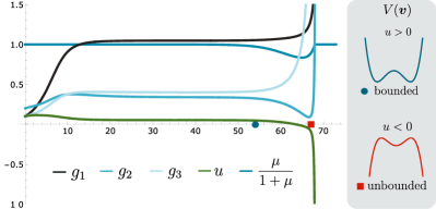
Figure 1: Renormalization group flow of the Malthusian Toner-Tu theory. In this example, the flow starts in the nearly incompressible regime, $\mu\gg 1$ and $\mu/(1+\mu)\simeq 1$; as soon as the flow escapes from the incompressible regime, the ferromagnetic coupling $u_{b}$ (green curve) becomes negative, and then the flow is characterized by run-away trajectories. In the $u_{b}<0$ regime the system is unstable. In the inserts we show qualitatively how the pseudo-potential $V(\bm{v})$ changes before (blue dot) and after (red square) the flow enters the unstable region; when $u_{b}$ becomes negative the pseudo-potential is unbounded.

In figure 2 (right) we show two Feynman diagrams that generate a $\bm{v}^{4}\bm{v}$ term in the equation of motion, which may stabilize the system in the $u_{b}<0$ region. Even if the coefficient $J_{b}$ becomes negative , a force term $-\mathcal{K}\bm{v}^{4}\bm{v}$ could still guarantee the stability of the equation of motion, provided that $\mathcal{K}>0$. Adding this novel force term in the equation of motion is equivalent to modifying the pseudo-potential $V_{\mathrm{new}}(\bm{v})$ as follows:

$$V_{\mathrm{new}}(\bm{v})=\frac{1}{2}m_{0}\bm{v}^{2}+\frac{1}{4}J_{0}\bm{v}^{4}+\frac{1}{6}\mathcal{K}_{0}\bm{v}^{6}$$ (31)

If $\mathcal{K}_{0}$ is zero, the potential $V(\bm{v})$ develops a non-zero minimum only for $m_{0}<0$; moreover, these minima are arbitrarily close to zero provided that $m_{0}$ is small enough. This scenario gives rise to the phenomenology of a second-order phase transition. Conversely, if $\mathcal{K}_{0}>0$, the potential $V$ may develop a minimum which is not close to zero when $J_{0}$ becomes negative. As shown in figure 2, when the constant $J_{0}$ becomes negative the potential may develop a global minimum far from $\bm{v}=0$, provided that both $m_{0}$ and $\mathcal{K}_{0}$ remain positive; this would result in a discontinuous, first-order, phase transition.

In the literature, this scenario, where one or more couplings become negative and then run away, is often, but not always Toner (1982); Dasgupta and Halperin (1981), related to a fluctuation-induced first-order transition. The Heisenberg model with cubic anisotropy and the scalar electrodynamics Amit and Martin-Mayor (2005) are two paradigmatic examples in which run-away trajectories result in a first-order phase transition. Non-perturbative techniques are often needed to prove that a run-away RG trajectory results in a first-order phase transition Oerding et al. (2000); Amit and Martin-Mayor (2005), but this is beyond the purposes of this perturbative RG calculation.

The stopping condition of the RG equations is determined by the correlation length $\xi$, or by the system size $L$. Depending on $\xi$, the RG flow may enter or not the unstable region. If the correlation length, or the system size, is small the RG flow does not enter the unstable region, and the system displays the phenomenology of a second-order phase transition, ruled by the incompressible active matter fixed point. Conversely, if the correlation length is large enough, the RG flow enters the $u_{b}<0$ region; when it happens because of the strong fluctuations, a phase transition, that should be second-order, becomes first-order Amit and Martin-Mayor (2005). In this sense, we call this phase transition a fluctuation-induced first-order phase transition Amit and Martin-Mayor (2005).

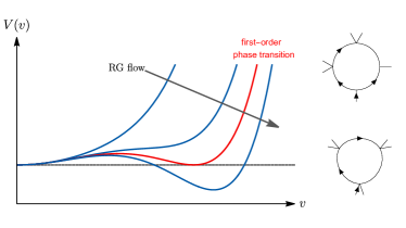
Figure 2: Left - An idea of how the inclusion of the $\bm{v}^{6}$ term in the potential, $V_{b}(\bm{v})=\frac{1}{2}m_{b}\bm{v}^{2}+\frac{1}{4}J_{b}\bm{v}^{4}+\frac{1}{6}\mathcal{K}_{b}\bm{v}^{6}$, may affect the renormalization group flow of the Malthusian Toner-Tu theory. $J_{b}$ becoming negative, while both $m_{b}$ and $\mathcal{K}_{b}$ staying positive, could lead to a first-order phase transition phenomenology. When the RG flow enters the $u_{b}<0$ region (red curve), the perturbative expansion breaks down. Right - Two of the 39 possible Feynman diagrams contributing to the generation of the coupling $\mathcal{K}_{0}\bm{v}^{4}\bm{v}$.

Conclusions - We computed the renormalization group flow for the Malthusian Toner-Tu theory. In the incompressible limit this calculation reproduces the results found in incompressible active matter Chen et al. (2015). Thus, in agreement with the numerical evidences Cavagna et al. (2021), the critical exponents found in Chen et al. (2015) hold also for systems with mild density fluctuations, provided that the correlation length (or the system size) is not too large. Furthermore, we found a relation between two measurable parameters, $\mu$ and the correlation length $\xi$ (or the size of the system $L$) that determines whether or not the critical dynamics is ruled by the incompressible active matter fixed point. If the system size is large enough, the RG flow escapes the incompressible active matter fixed point, and enters an unstable region. This suggests that, for large enough systems size $L$ and correlation length $\xi$, a fluctuation-induced first-order phase transition may occur; corroborating the idea that fluctuations and renormalization of parameters play a crucial role in determining the order of the phase transition Martin et al. (2021). We believe that even though, in MTT theory, density fluctuations are partially suppressed, they are still strong enough to turn the second-order phase transition into a first-order phase transition. Further studies are needed to clarify the situation; two strategies are including other couplings in the equation of motion or using non-perturbative techniques. This calculation provides one of the first RG evidence that the phase transition in active matter is first-order for large enough systems.

We thank A. Cavagna, I Giardina, and T. Grigera for discussions. We thank J. Toner and A. Maitra for comments. This work was supported by ERC grant RG.BIO (Grant No. 785932). L. Di Carlo designed the study, L. Di Carlo and M. Scandolo performed the RG computation.

References

- Vicsek et al. (1995) T. Vicsek, A. Czirók, E. Ben-Jacob, I. Cohen, and O. Shochet, Phys. Rev. Lett. 75, 1226 (1995).
- Vicsek and Zafeiris (2012) T. Vicsek and A. Zafeiris, Phys. Rep. 517, 71 (2012).
- Baglietto and Albano (2009) G. Baglietto and E. V. Albano, Phys. Rev. E 80, 50103 (2009).
- Chaté et al. (2008) H. Chaté, F. Ginelli, G. Grégoire, and F. Raynaud, Phys Rev E Stat Nonlin Soft Matter Phys 77, 46113 (2008).
- Solon et al. (2015) A. P. Solon, H. Chaté, and J. Tailleur, Phys. Rev. Lett. 114, 068101 (2015).
- Baglietto et al. (2012) G. Baglietto, E. V. Albano, and J. Candia, Interface Focus 2, 708 (2012).
- Ginelli (2016) F. Ginelli, Eur. Phys. J.: Spec. Top. 225, 2099 (2016).
- Martin et al. (2021) D. Martin, H. Chaté, C. Nardini, A. Solon, J. Tailleur, and F. Van Wijland, Phys. Rev. Lett. 126, 148001 (2021).
- Mishra and Mishra (2022) P. K. Mishra and S. Mishra, Active polar flock with birth and death (2022), arXiv:2201.10234 [cond-mat.soft] .
- Cates and Tailleur (2015) M. E. Cates and J. Tailleur, Annu. Rev. Condens. Matter Phys. 6, 219 (2015).
- Toner and Tu (1998) J. Toner and Y. Tu, Phys. Rev. E 58, 4828 (1998).
- Chen et al. (2015) L. Chen, J. Toner, and C. F. Lee, New J. Phys. 17, 42002 (2015).
- Cavagna et al. (2021) A. Cavagna, L. Di Carlo, I. Giardina, T. S. Grigera, and G. Pisegna, Phys. Rev. Res. 3, 10.1103/physrevresearch.3.013210 (2021).
- Toner (2012a) J. Toner, Phys. Rev. Lett. 108, 88102 (2012a).
- Landau and Lifshitz (1987) L. D. Landau and E. M. Lifshitz, Fluid mechanics: Landau and Lifshitz: course of theoretical physics (1987).
- Chen et al. (2020a) L. Chen, C. F. Lee, and J. Toner, Phys. Rev. E 102, 22610 (2020a).
- Ramaswamy (2010) S. Ramaswamy, Annu. Rev. Condens. Matter Phys. 1, 323 (2010).
- Chen et al. (2020b) L. Chen, C. F. Lee, J. Toner, and Others, Phys. Rev. Lett. 125, 98003 (2020b).
- Chen et al. (2020c) L. Chen, C. F. Lee, J. Toner, et al., Physical Review Letters 125, 098003 (2020c).
- Toner et al. (2005) J. Toner, Y. Tu, and S. Ramaswamy, Ann. Phys. 318, 170 (2005).
- Toner (2012b) J. Toner, Phys. Rev. E. Stat Nonlin Soft Matter Phys 86, 31918 (2012b).
- Cardy (1996) J. Cardy, Scaling and renormalization in statistical physics, Vol. 5 (Cambridge university press, 1996).
- Forster et al. (1977) D. Forster, D. R. Nelson, and M. J. Stephen, Phys. Rev. A 16, 10.1103/PhysRevA.16.732 (1977).
- Note (1) The effective coupling constant is linked to the coupling by the simple relation (22\@@italiccorr); therefore and have the same sign.
- Toner (1982) J. Toner, Phys. Rev. B 26, 462 (1982).
- Dasgupta and Halperin (1981) C. Dasgupta and B. I. Halperin, Phys. Rev. Lett. 47, 1556 (1981).
- Amit and Martin-Mayor (2005) D. J. Amit and V. Martin-Mayor, Field Theory, the Renormalization Group, and Critical Phenomena: Graphs to Computers Third Edition (World Scientific Publishing Company, 2005).
- Oerding et al. (2000) K. Oerding, F. Van Wijland, J. P. Leroy, and H. J. Hilhorst, J. Stat. Phys. 99, 1365 (2000), arXiv:9910351 [cond-mat] .