3PC: Three Point Compressors for Communication-Efficient Distributed Training and a Better Theory for Lazy Aggregation

Abstract

We propose and study a new class of gradient communication mechanisms for communication-efficient training—three point compressors (3PC)—as well as efficient distributed nonconvex optimization algorithms that can take advantage of them. Unlike most established approaches, which rely on a static compressor choice (e.g., Top-$K$), our class allows the compressors to evolve throughout the training process, with the aim of improving the theoretical communication complexity and practical efficiency of the underlying methods. We show that our general approach can recover the recently proposed state-of-the-art error feedback mechanism EF21 (Richtárik et al., 2021) and its theoretical properties as a special case, but also leads to a number of new efficient methods. Notably, our approach allows us to improve upon the state of the art in the algorithmic and theoretical foundations of the lazy aggregation literature (Chen et al., 2018). As a by-product that may be of independent interest, we provide a new and fundamental link between the lazy aggregation and error feedback literature. A special feature of our work is that we do not require the compressors to be unbiased.

1 Introduction

It has become apparent in the last decade that, other things equal, the practical utility of modern machine learning models grows with their size and with the amount of data points used in the training process. This big model and big data approach, however, comes with increased demands on the hardware, algorithms, systems and software involved in the training process.

1.1 Big data and the need for distributed systems

In order to handle the large volumes of data involved in training SOTA models, it is now absolutely necessary to rely on (often massively) distributed computing systems Dean et al. (2012); Khirirat et al. (2018); Lin et al. (2018). Indeed, due to storage and compute capacity limitations, large-enough training data sets can no longer be stored on a single machine, and instead need to be distributed across and processed by an often large number of parallel workers.

In particular, in this work we consider distributed supervised learning problems of the form

$$\textstyle\min\limits_{x\in\mathbb{R}^{d}}\left[f(x):=\frac{1}{n}\sum\limits_{i=1}^{n}f_{i}(x)\right],$$ (1)

where $n$ is the number of parallel workers/devices/clients, $x$ is a vector representing the $d$ parameters of a machine learning model (e.g., the weights in a neural network), and $f_{i}(x)$ is the loss of model $x$ on the training data stored on client $i\in[n]:=\{1,2,\dots,n\}$.

In some applications, as in federated learning (FL) McMahan et al. (2016); Konečný et al. (2016b; a); McMahan et al. (2017), the training data is captured in a distributed fashion in the first place, and there are reasons to process it in this decentralized fashion as well, as opposed to first moving it to a centralized location, such as a datacenter, and subsequently processing it there. Indeed, FL refers to machine learning in the environment where a large collection of highly heterogeneous clients (e.g., mobile devices, smart home appliances or corporations) tries to collaboratively train a model using the diverse data stored on these devices, but without compromising the clients’ data privacy.

1.2 Big model and the need for communication reduction

While distributing the data across several workers certainly alleviates the per-client storage and compute bottlenecks, the training task is obviously not fully decomposed this way. Indeed, the $n$ clients still need to work together to train the model, and working together means communication.

Since currently the most efficient training mechanisms rely on gradient-type methods Bottou (2012); Kingma & Ba (2014); Gorbunov et al. (2021), and since these operate by iteratively updating all the $d$ parameters describing the model, relying on big models leads to the need to communicate large-dimensional gradient vectors, which is expensive. For this reason, modern distributed methods need to rely on mechanisms that alleviate this communication burden.

Several orthogonal algorithmic approaches have been proposed in the literature to tackle this issue. One strain of methods, particularly popular in FL, is based on richer local training (e.g., LocalSGD), which typically means going beyond a single local gradient step before communication/aggregation across the workers is performed. This strategy is based on the hope that richer local training will ultimately lead to a dramatic reduction in the number of communication rounds without increasing the local computation time by much (Stich, 2020; Khaled et al., 2020; Woodworth et al., 2020). Another notable strain of methods is based on communication compression (e.g., QSGD), which means applying a lossy transformation to the communicated gradient information. This strategy is based on the hope that communication compression will lead to a dramatic reduction in the communication time within each round without affecting the number of communication rounds by much Khirirat et al. (2018); Alistarh et al. (2018); Mishchenko et al. (2019); Li et al. (2020); Li & Richtárik (2020; 2021).

1.3 Gradient descent with compressed communication

In this work we focus on algorithms based on the latter line of work: communication compression.

Perhaps conceptually the simplest yet versatile gradient-based method for solving the distributed problem (1) employing communication compression is distributed compressed gradient descent (DCGD) Khirirat et al. (2018). Given a sequence $\{\gamma^{t}\}$ of learning rates, DCGD performs the iterations

$$\textstyle x^{t+1}=x^{t}-\gamma^{t}\frac{1}{n}\sum\limits_{i=1}^{n}g_{i}^{t},\quad g_{i}^{t}={\cal M}_{i}^{t}(\nabla f_{i}(x^{t})).$$ (2)

Above, ${\cal M}_{i}^{t}$ represents any suitable gradient communication mechanism for mapping the possibly dense, high-dimensional, and hence hard-to-communicate gradient $\nabla f_{i}(x^{t})\in\mathbb{R}^{d}$ into a vector of equal dimension, but one that can hopefully be communicated using much fewer bits.

Table 1: Summary of the methods fitting our general 3PC framework. For each method we give the formula for the 3PC compressor $\mathcal{C}_{h,y}(x)$, its parameters ${\color[rgb]{0.75390625,0.18359375,0.09765625}A}$, ${\color[rgb]{0.75390625,0.18359375,0.09765625}B}$, and the ratio $\nicefrac{{{\color[rgb]{0.75390625,0.18359375,0.09765625}B}}}{{{\color[rgb]{0.75390625,0.18359375,0.09765625}A}}}$ appearing in the convergence rate. Notation: $\alpha$ = parameter of the contractive compressor $\mathcal{C}$, $\omega$ = parameter of the unbiased compressor $\mathcal{Q}$, ${\color[rgb]{0.75390625,0.18359375,0.09765625}A}_{1},{\color[rgb]{0.75390625,0.18359375,0.09765625}B}_{1}$ = parameters of three points compressor $\mathcal{C}_{h,y}^{1}(x)$, $\bar{\alpha}=1-(1-\alpha_{1})(1-\alpha_{2})$, where $\alpha_{1},\alpha_{2}$ are the parameters of the contractive compressors $\mathcal{C}_{1},\mathcal{C}_{2}$, respectively.

Variant of 3PC (Alg. 1)	Alg. #	$\mathcal{C}_{h,y}(x)=$	${\color[rgb]{0.75390625,0.18359375,0.09765625}A}$	${\color[rgb]{0.75390625,0.18359375,0.09765625}B}$	$\frac{{\color[rgb]{0.75390625,0.18359375,0.09765625}B}}{{\color[rgb]{0.75390625,0.18359375,0.09765625}A}}$
EF21 (Richtárik et al., 2021)	Alg. 2	$h+\mathcal{C}(x-h)$	$1-\sqrt{1-\alpha}$	$\frac{1-\alpha}{1-\sqrt{1-\alpha}}$	${\cal O}\left(\frac{1-\alpha}{\alpha^{2}}\right)$
LAG (Chen et al., 2018) (3)	Alg. 3	$\begin{cases}x,&\text{if }(\ast),\\ h,&\text{otherwise,}\end{cases}$ $(*)$ means $\|x-h\|^{2}>\zeta\|x-y\|^{2}$	$1$	$\zeta$	${\cal O}\left(\zeta\right)$
CLAG (NEW)	Alg. 4	$\begin{cases}h+\mathcal{C}(x-h),&\text{if }(\ast),\\ h,&\text{otherwise,}\end{cases}$ $(*)$ means $\|x-h\|^{2}>\zeta\|x-y\|^{2}$	$1-\sqrt{1-\alpha}$	$\max\left\{\frac{1-\alpha}{1-\sqrt{1-\alpha}},\zeta\right\}$	${\cal O}\left(\max\left\{\frac{1-\alpha}{\alpha^{2}},\frac{\zeta}{\alpha}\right\}\right)$
3PCv1 (NEW)	Alg. 5	$y+\mathcal{C}(x-y)$(1)	$1$	$1-\alpha$	$1-\alpha$
3PCv2 (NEW)	Alg. 6	$b+\mathcal{C}\left(x-b\right)$, where $b=h+\mathcal{Q}(x-y)$	$\alpha$	$(1-\alpha)\omega$	$\frac{(1-\alpha)\omega}{\alpha}$
3PCv3 (NEW)	Alg. 7	$b+\mathcal{C}\left(x-b\right)$, where $b=\mathcal{C}_{h,y}^{1}(x)$	$1-(1-\alpha)(1-{\color[rgb]{0.75390625,0.18359375,0.09765625}A}_{1})$	$(1-\alpha){\color[rgb]{0.75390625,0.18359375,0.09765625}B}_{1}$	$\frac{(1-\alpha){\color[rgb]{0.75390625,0.18359375,0.09765625}B}_{1}}{1-(1-\alpha)(1-{\color[rgb]{0.75390625,0.18359375,0.09765625}A}_{1})}$
3PCv4 (NEW)	Alg. 8	$b+\mathcal{C}_{1}\left(x-b\right)$, where $b=h+\mathcal{C}_{2}(x-h)$	$1-\sqrt{1-\bar{\alpha}}$	$\frac{1-\bar{\alpha}}{1-\sqrt{1-\bar{\alpha}}}$	${\cal O}\left(\frac{1-\bar{\alpha}}{\bar{\alpha}^{2}}\right)$
3PCv5 (NEW)	Alg. 9	$\begin{cases}x,&\text{w.p.\ }p\\ h+\mathcal{C}(x-y),&\text{w.p.\ }1-p\end{cases}$	$1-\sqrt{1-p}$	$\frac{(1-p)(1-\alpha)}{1-\sqrt{1-p}}$	${\cal O}\left(\frac{(1-p)(1-\alpha)}{p^{2}}\right)$
MARINA (Gorbunov et al., 2021)	Alg. 10	N/A(2)	$p$	$\frac{(1-p)\omega}{n}$	$\frac{(1-p)\omega}{np}$

• 3PCv1 requires communication of uncompressed vectors ($\nabla f_{i}(x^{t})$). Therefore, the method is impractical. We include it as an idealized version of EF21.

• MARINA does not fit the definition of three points compressor from (6). However, it satisfies (16) with $G^{t}=\|g^{t}-\nabla f(x^{t})\|^{2}$ and shown parameters ${\color[rgb]{0.75390625,0.18359375,0.09765625}A}$ and ${\color[rgb]{0.75390625,0.18359375,0.09765625}B}$, i.e., MARINA can be analyzed via our theoretical framework.

• LAG presented in our work is a (massively) simplified version of LAG considered by Chen et al. (2018). However, we have decided to use the same name.

Table 2: Comparison of exisiting and proposed theoretically-supported methods employing lazy aggregation. In the rates for our methods, $M_{1}=L_{-}+L_{+}\sqrt{\nicefrac{{{\color[rgb]{0.75390625,0.18359375,0.09765625}B}}}{{{\color[rgb]{0.75390625,0.18359375,0.09765625}A}}}}$ and $M_{2}=\max\left\{L_{-}+L_{+}\sqrt{\nicefrac{{2{\color[rgb]{0.75390625,0.18359375,0.09765625}B}}}{{{\color[rgb]{0.75390625,0.18359375,0.09765625}A}}}},\nicefrac{{{\color[rgb]{0.75390625,0.18359375,0.09765625}A}}}{{2\mu}}\right\}$.

Method	Simple method?	Uses a contractive compressor $\mathcal{C}$?	Strongly convex rate	PŁ nonconvex rate	General nonconvex rate
LAG (Chen et al., 2018)	✓	✗	linear (9)	✗	✗
LAQ (Sun et al., 2019)	✗	✓(1)	linear (3)	✗	✗
LENA (Ghadikolaei et al., 2021) (7)	✓(4)	✓(8)	${\cal O}(G^{4}/T^{2}\mu^{2})$ (5), (6)	${\cal O}(G^{4}/T^{2}\mu^{2})$ (5), (6)	${\cal O}(G^{4/3}/T^{2/3})$ (6)
LAG (NEW, 2022)	✓	✗	${\cal O}(\exp(-T\mu/M_{2}))$	${\cal O}(\exp(-T\mu/M_{2}))$	${\cal O}(M_{1}/T)$
CLAG (NEW, 2022)	✓	✓(2)	${\cal O}(\exp(-T\mu/M_{2}))$	${\cal O}(\exp(-T\mu/M_{2}))$	${\cal O}(M_{1}/T)$

• They consider a specific form of quantization only.

• Works with any contractive compressor, including low rank approximation, Top-$K$, Rand-$K$, quantization, and more.

• Their Theorem 1 does not present any explicit linear rate.

• LENA employs the classical EF mechanism, but it is not clear what is this mechanism supposed to do.

• They consider an assumption ($\mu$-quasi-strong convexity) that is slightly stronger than our PŁ assumption. Both are weaker than strong convexity.

• They assume the local gradients to be bounded by $G$ ($\|\nabla f_{i}(x)\|\leq G$ for all $x$). We do not need such a strong assumption.

• They also consider the $0$-quasi-strong convex case (slight generalization of convexity); we do not consider the convex case. Moreover, they consider the stochastic case as well, we do not. We specialized all their results to the deterministic (i.e., full gradient) case for the purposes of this table.

• Their contractive compressor depends on the trigger.

• It is possible to specialize their method and proof so as to recover LAG as presented in our work, and to recover a rate similar to ours.

2 Motivation and Background

Our work is motivated by several methodological, theoretical and algorithmic issues and open problems arising in the literature related to two orthogonal approaches to designing gradient communication mechanisms ${\cal M}_{i}^{t}$:

• contractive compressors Karimireddy et al. (2019); Stich et al. (2018); Alistarh et al. (2018); Koloskova et al. (2020); Beznosikov et al. (2020), and

• lazy aggregation Chen et al. (2018); Sun et al. (2019); Ghadikolaei et al. (2021).

The motivation for our work starts with several critical observations related to these two mechanisms.

2.1 Contractive compression operators

Arguably, the simplest class of communication mechanisms is based on the (as we shall see, naive) application of contractive compression operators (or, contractive compressors for short) Koloskova et al. (2020); Beznosikov et al. (2020). In this approach, one sets

$${\cal M}_{i}^{t}(x)\equiv\mathcal{C}(x),$$ (3)

where $\mathcal{C}:\mathbb{R}^{d}\to\mathbb{R}^{d}$ is a (possibly randomized) mapping with the property

$${\mathbb{E}}\left[\left\|\mathcal{C}(x)-x\right\|^{2}\right]\leq(1-\alpha)\left\|x\right\|^{2},\quad\forall x\in\mathbb{R}^{d},$$ (4)

where $0<\alpha\leq 1$ is the contraction parameter, and the expectation ${\mathbb{E}}\left[\cdot\right]$ is taken w.r.t. the randomness inherent in $\mathcal{C}$. For examples of contractive compressors (e.g., Top-$K$ and Rand-$K$ sparsifiers), please refer to Section A, and Table 1 in (Safaryan et al., 2021b; Beznosikov et al., 2020).

The algorithmic literature on contractive compressors (i.e., mappings $\mathcal{C}$ satisfying (4)) is relatively much more developed, and dates back to at least 2014 with the work of Seide et al. (2014), who proposed the error feedback (EF) mechanism for fixing certain divergence issues which arise empirically with the naive approach based on (3).

Despite several advances in our theoretical understanding of EF over the last few years Stich et al. (2018); Karimireddy et al. (2019); Horváth & Richtárik (2021); Tang et al. (2020); Gorbunov et al. (2020), a satisfactory grasp of EF remained elusive. Recently, Richtárik et al. (2021) proposed EF21, which is a new algorithmic and analysis approach to error feedback, effectively fixing the previous weaknesses. In particular, while previous results offered weak ${\cal O}(1/T^{2/3})$ rates (for smooth nonconvex problems), and did so under strong and often unrealistic assumptions (e.g., boundedness of the gradients), the EF21 approach offers GD-like ${\cal O}(1/T)$ rates, with standard assumptions only.

The heart of the EF21 method is a new communication mechanism ${\cal M}_{i}^{t}$, generated from a contractive compressor $\mathcal{C}$, which fixes (in a theoretically and practically superior way to the standard fix offered by classical EF) the above mentioned divergence issues. Their construction is synthetic: is starts with the choice of $\mathcal{C}$ preferred by the user, and then constructs a new and adaptive communication mechanism based on it. We will describe this method in Section 4.

2.2 Lazy aggregation

An orthogonal approach to applying contractive operators, whether with or without error feedback, is “skipping” communication. The basic idea of the lazy aggregation communication mechanism is for each worker $i$ to communicate its local gradient only if it differs “significantly” from the last gradient communicated before.

In its simplest form, the LAG method of Chen et al. (2018) is initialized with $g_{i}^{0}=\nabla f_{i}(x^{0})$ for all $i\in[n]$, which means that all the workers communicate their gradients at the start. In all subsequent iterations, each worker $i\in[n]$ defines $g_{i}^{t+1}$, which may be interpreted as a “compressed” version of the true gradient $\nabla f_{i}(x^{t+1})$, via the lazy aggregation rule

$$g_{i}^{t+1}=\begin{cases}\nabla f_{i}(x^{t+1})&\text{if }\|g_{i}^{t}-\nabla f_{i}(x^{t+1})\|^{2}>\zeta D_{i}^{t},\\ g_{i}^{t}&\text{otherwise,}\end{cases}$$ (5)

where $D_{i}^{t}:=\|\nabla f_{i}(x^{t+1})-\nabla f_{i}(x^{t})\|^{2}$ and $\zeta>0$ is the trigger. The smaller the trigger $\zeta$, the more likely it is for the condition $\|g_{i}^{t}-\nabla f_{i}(x^{t+1})\|^{2}>\zeta D_{i}^{t}$, which triggers communication, to be satisfied. On the other hand, if $\zeta$ is very large, most iterations will skip communication and thus reuse the past gradient. Since the trigger fires dynamically based on conditions that change in time, it is hard to theoretically estimate how often communication skipping occurs. In fact, there are no results on this in the literature. Nevertheless, the lazy aggregation mechanism is empirically useful when compared to vanilla GD (Chen et al., 2018).

Lazy aggregation is a much less studied and a much less understood communication mechanism than contractive compressors. Indeed, only a handful of papers offer any convergence guarantees (Chen et al., 2018; Sun et al., 2019; Ghadikolaei et al., 2021), and the results presented in the first two of these papers are hard to penetrate. For example, no simple proof exists for the simple LAG variant presented above. The best known rate in the smooth nonconvex regime is ${\cal O}(1/T^{2/3})$, which differs from the ${\cal O}(1/T)$ rate of GD. The known rates in the strongly convex regime are also highly problematic: they are either not explicit (Chen et al., 2018; Sun et al., 2019), or sublinear (Ghadikolaei et al., 2021). Furthermore, it is not clear whether an EF mechanism is needed to stabilize lazy aggregation methods, which is a necessity in the case of contractive compressors. While Ghadikolaei et al. (2021) proposed a combination of LAG and EF, their analysis leads to weak rates (see Table 2), and does not seem to point to theoretical advantages due to EF.

3 Summary of Contributions

We now summarize our main contributions:

$\bullet$ Unification through the 3PC method. At present, the two communication mechanisms outlined above, contractive compressors and lazy aggregation, are viewed as different approaches to the same problem—reducing the communication overhead in distributed gradient-type methods—requiring different tools, and facing different theoretical challenges. We propose a unified method—which we call 3PC (Algorithm 1)—which includes EF21 (Algorithm 2) and LAG (Algorithm 3) as special cases.

$\bullet$ Several new methods. The 3PC method is much more general than either EF21 or LAG, and includes a number of new specific methods. For example, we propose CLAG, which is a combination of EF21 and LAG benefiting from both contractive compressors and lazy aggregation. We show experimentally that CLAG can be better than both EF21 and LAG: that is, we obtain combined benefits of both approaches. We obtain a number of other new methods, such as 3PCv2, 3PCv3 and 3PCv4. We show experimentally that 3PCv2 can outperform EF21. See Table 1 for a summary of the proposed methods.

$\bullet$ Three point compressors. Our proposed method, 3PC, can be viewed as DCGD with a new class of communication mechanisms, based on the new notion of a three point compressor (3PC); see Section 4 for details. By design, and in contrast to contractive compressors, our communication mechanism based on the 3PC compressor is able to “evolve” and thus improve throughout the iterations. In particular, its compression error decays, which is the key reason behind its superior theoretical properties. In summary, the properties defining the 3PC compressor distill the important characteristics of a theoretically well performing communication mechanism, and this is the first time such characteristics have been explicitly identified and formalized.

The observation that lazy aggregation is a 3PC compressor explains why error feedback is not needed to stabilize LAG and similar methods.

$\bullet$ Strong rates. We prove an ${\cal O}(1/T)$ rate for 3PC for smooth nonconvex problems, which up to constants matches the rate of GD. Furthermore, we prove a GD-like linear convergence rate under the Polyak-Łojasiewicz condition. Our general theory recovers the EF21 rates proved by Richtárik et al. (2021) exactly. Our rates for lazily aggregated methods (LAG and CLAG) are new, and better than the results obtained by Chen et al. (2018); Sun et al. (2019) and Ghadikolaei et al. (2021) in all regimes considered. In the general smooth nonconvex regime, only Ghadikolaei et al. (2021) obtain rates. However, they require strong assumptions (gradients bounded by a constant $G$), and their rate is ${\cal O}(G^{4/3}/T^{2/3})$, whereas we do not need such assumptions and obtain the GD-like rate ${\cal O}(M_{1}/T)$. In the strongly convex regime, Chen et al. (2018) and Sun et al. (2019) obtain non-specific linear rates, while Ghadikolaei et al. (2021) obtain the sublinear rate ${\cal O}(G^{4}/T^{2}\mu^{2})$. In contrast, we obtain explicit GD-like linear rates under the weaker PŁ condition.

Furthermore, our variant of LAG, and our convergence theory and proofs, are much simpler than those presented in (Chen et al., 2018). In fact, it is not clear to us whether the many additional features employed by Chen et al. (2018) have any theoretical or practical benefits. We believe that our simple treatment can be useful for other researchers to further advance the field.

For a detailed comparison of rates, please refer to Table 2.

Algorithm 1 3PC (DCGD method using the 3PC communication mechanism)

1:  Input: starting point $x^{0}\in\mathbb{R}^{d}$ (on all workers), stepsize $\gamma>0$, number of iterations $T$, starting vectors $g_{i}^{0}\in\mathbb{R}^{d}$ for $i\in[n]$ (known to the server and all workers)

2:  Initialization: $g^{0}=\frac{1}{n}\sum_{i=1}^{n}g_{i}^{0}$ (Server aggregates initial gradient estimates)

3:  for $t=0,1,\ldots,T-1$ do

4:     Broadcast $g^{t}$ to all workers

5:     for $i=1,\ldots,n$ in parallel do

6:        $x^{t+1}=x^{t}-\gamma g^{t}$ (Take a gradient-type step)

7:        Set $g_{i}^{t+1}={\cal M}_{i}^{t+1}(\nabla f_{i}(x^{t+1})):=\mathcal{C}_{g_{i}^{t},\nabla f_{i}(x^{t})}(\nabla f_{i}(x^{t+1}))$ (Apply 3PC to compress the latest gradient)

8:        Communicate $g_{i}^{t+1}$ to the server

9:     end for

10:     Server aggregates received messages: $g^{t+1}=\tfrac{1}{n}\sum_{i=1}^{n}g_{i}^{t+1}$

11:  end for

12:  Return: $\hat{x}^{T}$ chosen uniformly at random from $\{x^{t}\}_{t=0}^{T-1}$

4 Three Point Compressors

We now formally introduce the concept of a three point compressor (3PC).

Definition 4.1 (Three point compressor).

We say that a (possibly randomized) map

$$\mathcal{C}_{h,y}(x):\underbrace{\mathbb{R}^{d}}_{h\in}\times\underbrace{\mathbb{R}^{d}}_{y\in}\times\underbrace{\mathbb{R}^{d}}_{x\in}\rightarrow\mathbb{R}^{d}$$

is a three point compressor (3PC) if there exist constants $0<{\color[rgb]{0.75390625,0.18359375,0.09765625}A}\leq 1$ and ${\color[rgb]{0.75390625,0.18359375,0.09765625}B}\geq 0$ such that the following relation holds for all $x,y,h\in\mathbb{R}^{d}$

$${\mathbb{E}}\left[\left\|\mathcal{C}_{h,y}(x)-x\right\|^{2}\right] \leq (1-{\color[rgb]{0.75390625,0.18359375,0.09765625}A})\left\|h-y\right\|^{2}$$ (6)

$$\quad+{\color[rgb]{0.75390625,0.18359375,0.09765625}B}\left\|x-y\right\|^{2}.$$

The vectors $y\in\mathbb{R}^{d}$ and $h\in\mathbb{R}^{d}$ are parameters defining the compressor. Once fixed, $\mathcal{C}_{h,y}:\mathbb{R}^{d}\to\mathbb{R}^{d}$ is the compression mapping used to compress vector $x\in\mathbb{R}^{d}$.

4.1 Connection with contractive compressors

Note that if we set $h=0$ and $y=x$, then inequality (6) specializes to

$${\mathbb{E}}\left[\left\|\mathcal{C}_{0,x}(x)-x\right\|^{2}\right] \leq (1-{\color[rgb]{0.75390625,0.18359375,0.09765625}A})\left\|x\right\|^{2},$$ (7)

which is the inequality defining a contractive compressor. In other words, a particular restriction of the parameters of any 3PC compressor is necessarily a contractive compressor.

However, this is not the restriction we will use to design our compression mechanism. Instead, as we shall describe next, we will choose the sequence of vectors $h$ and $y$ in an adaptive fashion, based on the path generated by DCGD.

4.2 Designing a communication mechanism using a 3PC compressor

We now describe our proposal for how to use a 3PC compressor to design a good communication mechanism $\{{\cal M}_{i}^{k}\}$ to be used within DCGD. Recall from (2) that all we need to do is to define the mapping

$${\cal M}_{i}^{t}:\nabla f_{i}(x^{t})\mapsto g_{i}^{t}.$$

First, we allow the initial compressed gradients $\{g_{i}^{0}\}_{i=1}^{n}$ to be chosen arbitrarily. Here are some examples of possible choices: a) Full gradients: $g_{i}^{0}=\nabla f_{i}(x^{0})$ for all $i\in[n]$. The benefit of this choice is that no information is loss at the start of the process. On the other hand, the full $d$-dimensional gradients need to be sent by the workers to the server, which is potentially an expensive pre-processing step. b) Compressed gradients: $g_{i}^{0}=\mathcal{C}(\nabla f_{i}(x^{0}))$ for all $i\in[n]$, where $\mathcal{C}$ is an arbitrary compression mapping (e.g., a contractive compressor). While some information is lost right at the start of the process (compared to a GD step), the benefit of this choice is that no full dimensional vectors need to be communicated. c) Zero preprocessing: $g_{i}^{0}=0$ for all $i\in[n]$.

Having chosen $g_{i}^{0},\dots,g_{i}^{0}$ for all $i\in[n]$, it remains to define the communication mechanism ${\cal M}_{i}^{t}$ for $t\geq 1$. We will do this on-the-fly as DCGD is run, with the help of the parameters $h$ and $y$, which we choose adaptively. Consider the viewpoint of a worker $i\in[n]$ in iteration $t+1$, with $t\geq 0$. In this iteration, worker $i$ wishes to compress the vector $x=\nabla f_{i}(x^{t+1})$. Let $g_{i}^{t}$ denote the compressed version of the vector $\nabla f_{i}(x^{t})$, i.e., $g_{i}^{t}={\cal M}_{i}^{t}(\nabla f_{i}(x^{t}))$. We choose

$$y=\nabla f_{i}(x^{t})\qquad\text{and}\qquad h=g_{i}^{t}.$$

With these parameter choices, we define the compressed version of $x=\nabla f_{i}(x^{t+1})$ by setting

$${\cal M}_{i}^{t+1}(\nabla f_{i}(x^{t+1}))\overset{\eqref{eq:DCGD}}{=}g_{i}^{t+1}:=\mathcal{C}_{g_{i}^{t},\nabla f_{i}(x^{t})}(\nabla f_{i}(x^{t+1})).$$ (8)

Our porposed 3PC method (Algorithm 1) is just DCGD with the compression mechanism described above.

4.3 The 3PC inequality

For the parameter choices made above, (6) specializes to

$${\mathbb{E}}\left[E_{i}^{t+1}\;|\;x^{t},g_{i}^{t}\right]\leq(1-{\color[rgb]{0.75390625,0.18359375,0.09765625}A})E_{i}^{t}+{\color[rgb]{0.75390625,0.18359375,0.09765625}B}D_{i}^{t},$$ (9)

where

$$E_{i}^{t}:=\left\|g_{i}^{t}-\nabla f_{i}(x^{t})\right\|^{2}$$

and

$$D_{i}^{t}:=\left\|\nabla f_{i}(x^{t+1})-\nabla f_{i}(x^{t})\right\|^{2}.$$

This inequality has a natural interpretation. It enforces the compression error $E_{i}^{t}$ to shrink by the factor of $1-{\color[rgb]{0.75390625,0.18359375,0.09765625}A}$ in each communication round, subject to an additive penalty proportional to $D_{i}^{t}$. If the iterates converge, then the penalty will eventually vanish as well provided that the gradient of $f_{i}$ is continuous. Intuitively speaking, this forces the compression error $E^{t}$ to improve in time.

We note that applying a simple contractive compressor in place of ${\cal M}_{i}^{t}$ does not have this favorable property, and this is what causes the convergence issues in existing literature on this topic. This is what the EF literature was trying to solve since 2014, and what the EF21 mechanism resolved in 2021. However, no such progress happened in the lazy aggregation literature yet, and one of the key contributions of our work is to remedy this situation.

4.4 EF21 mechanism is a 3PC compressor

We will now show that the compression mechanism ${\cal M}_{i}^{t}$ employed in EF21 comes from a 3PC compressor. Let $\mathcal{C}:\mathbb{R}^{d}\to\mathbb{R}^{d}$ be a contractive compressor with contraction parameter $\alpha$, and define

$$\mathcal{C}_{h,y}(x):=h+\mathcal{C}(x-h).$$ (10)

If we use this mapping to define a compression mechanism ${\cal M}_{i}^{t}$ via (8), use this within DCGD, we obtain the EF21 method of Richtárik et al. (2021). Indeed, observe that Algorithm 2 (EF21) is a special case of Algorithm 1 (3PC).

The next lemma shows that (10) is a 3PC compressor.

Lemma 4.2.

The mapping (10) satisfies (6) with ${\color[rgb]{0.75390625,0.18359375,0.09765625}A}:=1-(1-\alpha)(1+s)$ and ${\color[rgb]{0.75390625,0.18359375,0.09765625}B}:=(1-\alpha)\left(1+s^{-1}\right)$, where $s>0$ is any scalar satisfying $(1-\alpha)\left(1+s\right)<1$.

4.5 LAG mechanism is a 3PC compressor

We will now show that the compression mechanism ${\cal M}_{i}^{t}$ employed in LAG comes from a 3PC compressor. In fact, let us define CLAG, and recover LAG from it as a special case. Let $\mathcal{C}:\mathbb{R}^{d}\to\mathbb{R}^{d}$ be a contractive compressor with contraction parameter $\alpha$. Choose a trigger $\zeta>0$, and define

$$\mathcal{C}_{h,y}(x):=\begin{cases}h+\mathcal{C}(x-h),&\text{if }\|x-h\|^{2}>\zeta\|x-y\|^{2},\\ h,&\text{otherwise,}\end{cases}$$ (11)

If we use this mapping to define a compression mechanism ${\cal M}_{i}^{t}$ via (8), use this within DCGD, we obtain our new CLAG method. Indeed, observe that Algorithm 4 (CLAG) is a special case of Algorithm 1 (3PC).

The next lemma shows that (11) is a 3PC compressor.

Lemma 4.3.

The mapping (11) satisfies (6) with ${\color[rgb]{0.75390625,0.18359375,0.09765625}A}:=1-(1-\alpha)(1+s)$ and ${\color[rgb]{0.75390625,0.18359375,0.09765625}B}:=\max\left\{(1-\alpha)\left(1+s^{-1}\right),\zeta\right\}$, where $s>0$ is any scalar satisfying $(1-\alpha)\left(1+s\right)<1$.

The LAG method is obtained as a special case of CLAG by choosing $\mathcal{C}$ to be the identity mapping (for which $\alpha=1$).

4.6 Further 3PC compressors and methods

In Table 1 we summarize several further 3PC compressors and the new algorithms they lead to (e.g., 3PCv1–3PCv5). The details are given the in the appendix.

5 Theory

We are now ready to present our theoretical convergence results for the 3PC method (Algorithm 1), the main steps of which are

$$\textstyle x^{t+1}=x^{t}-\gamma g^{t},\quad g^{t}=\frac{1}{n}\sum\limits_{i=1}^{n}g_{i}^{t},$$ (12)

$$g_{i}^{t+1}=\mathcal{C}_{g_{i}^{t},\nabla f_{i}(x^{t})}(\nabla f_{i}(x^{t+1})).$$ (13)

Recall that the 3PC method is DCGD with a particular choice of the communication mechanism $\{{\cal M}_{i}^{t}\}$ based on an arbitrary 3PC compressor $\mathcal{C}_{h,y}(x)$.

5.1 Assumptions

We rely on the following standard assumptions.

Assumption 5.1.

The functions $f_{1},\dots,f_{n}:\mathbb{R}^{d}\to\mathbb{R}$ are differentiable. Moreover, $f$ is lower bounded, i.e., there exists $f^{\inf}\in\mathbb{R}$ such that $f(x)\geq f^{\inf}$ for all $x\in\mathbb{R}^{d}$.

Assumption 5.2.

The function $f:\mathbb{R}^{d}\to\mathbb{R}$ is $L_{-}$-smooth, i.e., it is differentibale and its gradient satisfies

$$\|\nabla f(x)-\nabla f(y)\|\leq L_{-}\|x-y\|\quad\forall x,y\in\mathbb{R}^{d}.$$ (14)

Assumption 5.3.

There is a constant $L_{+}>0$ such that $\frac{1}{n}\sum_{i=1}^{n}\left\|\nabla f_{i}(x)-\nabla f_{i}(y)\right\|^{2}\leq L^{2}_{+}\left\|x-y\right\|^{2}$ for all $x,y\in\mathbb{R}^{d}$. Let $L_{+}$ be the smallest such number.

It is easy to see that $L_{-}\leq L_{+}$. We borrow this notation for the smoothness constants from (Szlendak et al., 2021).

5.2 Convergence for general nonconvex functions

The following lemma is based on the properties of the 3PC compressor. It establishes the key inequality for the convergence analysis. The proof follows easily from the definition of a 3PC compressor and Assumption 5.3.

Lemma 5.4.

Let Assumption 5.3 hold. Consider the 3PC method. Then, the sequence

$$\textstyle G^{t}:=\frac{1}{n}\sum\limits_{i=1}^{n}\left\|g_{i}^{t}-\nabla f_{i}(x^{t})\right\|^{2}$$ (15)

for all $t\geq 0$ satisfies

$$\textstyle{\mathbb{E}}\left[G^{t+1}\right]\leq(1-{\color[rgb]{0.75390625,0.18359375,0.09765625}A}){\mathbb{E}}\left[G^{t}\right]+{\color[rgb]{0.75390625,0.18359375,0.09765625}B}L_{+}^{2}{\mathbb{E}}\left[\left\|x^{t+1}-x^{t}\right\|^{2}\right].$$ (16)

Using this lemma and arguments from the analysis of SGD for non-convex problems (Li et al., 2021; Richtárik et al., 2021), we derive the following result.

Theorem 5.5.

Let Assumptions 5.1, 5.2, 5.3 hold. Assume that the stepsize $\gamma$ of the 3PC method satisfies $0\leq\gamma\leq\nicefrac{{1}}{{M_{1}}}$, where $M_{1}=L_{-}+L_{+}\sqrt{\nicefrac{{{\color[rgb]{0.75390625,0.18359375,0.09765625}B}}}{{{\color[rgb]{0.75390625,0.18359375,0.09765625}A}}}}$. Then, for any $T\geq 1$ we have

$$\textstyle{\mathbb{E}}\left[\left\|\nabla f(\hat{x}^{T})\right\|^{2}\right]\leq\frac{2\Delta^{0}}{\gamma T}+\frac{{\mathbb{E}}\left[G^{0}\right]}{{\color[rgb]{0.75390625,0.18359375,0.09765625}A}T},$$ (17)

where $\hat{x}^{T}$ is sampled uniformly at random from the points $\{x^{0},x^{1},\ldots,x^{T-1}\}$ produced by 3PC , $\Delta^{0}:=f(x^{0})-f^{\inf}$, and $G^{0}$ is defined in (15).

The theorem implies the following fact.

Corollary 5.6.

Let the assumptions of Theorem 5.5 hold and choose the stepsize

$$\textstyle\gamma=\frac{1}{L_{-}+L_{+}\sqrt{\nicefrac{{{\color[rgb]{0.75390625,0.18359375,0.09765625}B}}}{{{\color[rgb]{0.75390625,0.18359375,0.09765625}A}}}}}.$$

Then for any $T\geq 1$ we have

$$\textstyle{\mathbb{E}}\left[\left\|\nabla f(\hat{x}^{T})\right\|^{2}\right]\leq\frac{2\Delta^{0}\left(L_{-}+L_{+}\sqrt{\nicefrac{{{\color[rgb]{0.75390625,0.18359375,0.09765625}B}}}{{{\color[rgb]{0.75390625,0.18359375,0.09765625}A}}}}\right)}{T}+\frac{{\mathbb{E}}\left[G^{0}\right]}{{\color[rgb]{0.75390625,0.18359375,0.09765625}A}T}.$$

That is, to achieve ${\mathbb{E}}\left[\left\|\nabla f(\hat{x}^{T})\right\|^{2}\right]\leq\varepsilon^{2}$ for some $\varepsilon>0$, the 3PC method requires

$$\textstyle T={\cal O}\left(\frac{\Delta^{0}\left(L_{-}+L_{+}\sqrt{\nicefrac{{{\color[rgb]{0.75390625,0.18359375,0.09765625}B}}}{{{\color[rgb]{0.75390625,0.18359375,0.09765625}A}}}}\right)}{\varepsilon^{2}}+\frac{{\mathbb{E}}\left[G^{0}\right]}{{\color[rgb]{0.75390625,0.18359375,0.09765625}A}\varepsilon^{2}}\right)$$ (18)

iterations (=communication rounds).

5.3 Convergence under the PŁ condition

In this part we provide our main convergence result under the Polyak-Łojasiewicz (PŁ) condition.

Assumption 5.7 (PŁ condition).

Function $f:\mathbb{R}^{d}\to\mathbb{R}$ satisfies the Polyak-Łojasiewicz (PŁ) condition with parameter $\mu>0$, i.e.,

$$\|\nabla f(x)\|^{2}\geq 2\mu\left(f(x)-f^{*}\right),\quad\forall x\in\mathbb{R}^{d},$$ (19)

where $x^{*}:=\operatorname*{arg\,min}_{x\in\mathbb{R}^{d}}f(x)$ and $f^{*}:=f(x^{*})$.

In this setting, we get the following result.

Theorem 5.8.

Let Assumptions 5.1, 5.2, 5.3, 5.7 hold. Assume that the stepsize $\gamma$ of the 3PC method satisfies $0\leq\gamma\leq\nicefrac{{1}}{{M_{2}}}$, where $M_{2}=\max\left\{L_{-}+L_{+}\sqrt{\nicefrac{{2{\color[rgb]{0.75390625,0.18359375,0.09765625}B}}}{{{\color[rgb]{0.75390625,0.18359375,0.09765625}A}}}},\nicefrac{{{\color[rgb]{0.75390625,0.18359375,0.09765625}A}}}{{2\mu}}\right\}$. Then, for any $T\geq 0$ and $\Delta^{0}:=f(x^{0})-f(x^{*})$ we have

$$\textstyle{\mathbb{E}}\left[f(x^{T})\right]-f^{*}\leq\left(1-\gamma\mu\right)^{T}\left(\Delta^{0}+\frac{\gamma}{{\color[rgb]{0.75390625,0.18359375,0.09765625}A}}{\mathbb{E}}\left[G^{0}\right]\right).$$ (20)

The theorem implies the following fact.

Corollary 5.9.

Let the assumptions of Theorem 5.8 hold and choose the stepsize

$$\textstyle\gamma=\min\left\{\frac{1}{L_{-}+L_{+}\sqrt{\nicefrac{{2{\color[rgb]{0.75390625,0.18359375,0.09765625}B}}}{{{\color[rgb]{0.75390625,0.18359375,0.09765625}A}}}}},\frac{{\color[rgb]{0.75390625,0.18359375,0.09765625}A}}{2\mu}\right\}.$$

Then to achieve ${\mathbb{E}}\left[f(x^{T})\right]-f^{*}\leq\varepsilon$ for some $\varepsilon>0$ the method requires

$$\textstyle{\cal O}\left(\max\left\{\frac{L_{-}+L_{+}\sqrt{\nicefrac{{{\color[rgb]{0.75390625,0.18359375,0.09765625}B}}}{{{\color[rgb]{0.75390625,0.18359375,0.09765625}A}}}}}{\mu},{\color[rgb]{0.75390625,0.18359375,0.09765625}A}\right\}\log\frac{\Delta^{0}+{\mathbb{E}}\left[G^{0}\right]\nicefrac{{\gamma}}{{{\color[rgb]{0.75390625,0.18359375,0.09765625}A}}}}{\varepsilon}\right)$$ (21)

iterations (=communication rounds).

5.4 Commentary

As mentioned in the contributions section, the above rates match those of GD in the considered regimes, up to constants factors, and at present constitute the new best-known rates for methods based on lazy aggregation. They recover the best known rates for error feedback since they match the rate of EF21.

6 Experiments

Now we empirically test the new variants of 3PC in two expriments. In the first experiment, we focus on compressed lazy aggregation mechanism and study the behavior of CLAG (Algorithm 4) combined with Top-$K$ compressor. In the second one, we compare 3PCv2 (Algorithm 6) to EF21 with Top-$K$ on a practical task of learning a representation of MNIST dataset LeCun et al. (2010).

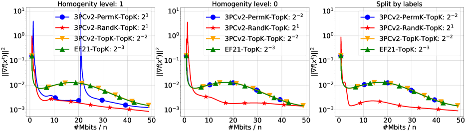
Figure 1: Comparison of 3PCv2 with Perm-$K$, Rand-$K$ and Top-$K$ as the first compressor. Top-$K$ is used as the second compressor. Number of clients $n=100$, compression level $K=251$. EF21 with Top-$K$ is provided for the reference.

6.1 Is CLAG better than LAG and EF21?

Consider solving the non-convex logistic regression problem

$$\textstyle\min\limits_{x\in\mathbb{R}^{d}}\left[f(x):=\frac{1}{N}\sum\limits_{i=1}^{N}\log(1+e^{-y_{i}a_{i}^{\top}x})+\lambda\sum\limits_{j=1}^{d}\frac{x_{j}^{2}}{1+x_{j}^{2}}\right],$$

where $a_{i}\in\mathbb{R}^{d}$, $y_{i}\in\{-1,1\}$ are the training data and labels, and $\lambda>0$ is a regularization parameter, which is fixed to $\lambda=0.1$. We use four LIBSVM Chang & Lin (2011) datasets phishing, w6a, a9a, ijcnn1 as training data. Each dataset is shuffled and split into $n=20$ equal parts.

We vary two parameters of CLAG, $K$ and $\zeta$, and report the number of bits (per worker) sent from clients to the server to achieve $\|\nabla f(x^{t})\|<10^{-2}$. For each pair ($K$, $\zeta$), we fine-tune the stepsize of CLAG with multiples ($1,2^{1},2^{2},\dots,2^{11}$) of the theoretical stepsize. We report the results on a heatmap (see Figure 2) for the representative dataset ijcnn1. Other datasets are included in Appendix E. On the heatmap, we vary $\zeta$ along rows and $K$ along columns. Notice that CLAG reduces to LAG when $K=d$ (bottom row) and to EF21 when $\zeta=0$ (left column).

The experiment shows that the minimum communication complexity is attained at a combination of $(K,\zeta)$, which does not reduce CLAG to its special cases: EF21 or LAG. This empirically confirms that CLAG has better communication complexity than EF21 and LAG.

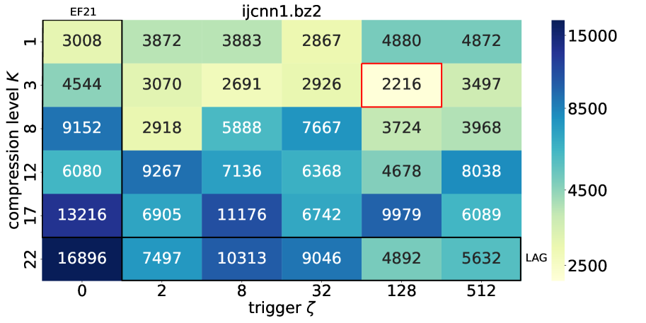
Figure 2: Heatmap of communication complexities of CLAG for different combination of compression levels $K$ and triggers $\zeta$ with tuned stepsizes on ijcnn1 dataset. We contour cells corresponding to EF21 and LAG, as special cases of CLAG, by black rectangles. The red-contoured cell indicates the experiment with the smallest communication cost.

Additional experiments validating the performance of CLAG are reported in Appendix E

6.2 Other 3PC variants

We consider the objective

$$\min_{\boldsymbol{D}\in\mathbb{R}^{d_{f}\times d_{e}},\boldsymbol{E}\in\mathbb{R}^{d_{e}\times d_{f}}}\left[f(\boldsymbol{D},\boldsymbol{E}):=\frac{1}{N}\sum_{i=1}^{N}\left\|\boldsymbol{D}\boldsymbol{E}a_{i}-a_{i}\right\|^{2}\right],$$

where $a_{i}$ are flattened represenations of images with $d_{f}=784$, $\boldsymbol{D}$ and $\boldsymbol{E}$ are learned parameters of the autoencoder model. We fix the encoding dimensions as $d_{e}=16$ and distribute the data samples across $n=100$ clients. In order to control the heterogenity of this distribution, we consider three cases. First, each client owns the same data (“homogeneity level: $1$”). Second, the data is randomly split among client (“homogeneity level: $0$”). Finally, we consider an extremely heterogeneous case, where the images are “split by labels”. $K$ is set to $\nicefrac{{d}}{{n}}$, where $d=2\cdot d_{f}\cdot d_{e}=25088$ is the total dimension of learning parameters $\boldsymbol{D}$ and $\boldsymbol{E}$. We apply three different sparsifiers (Top-$K$, Rand-$K$, Perm-$K$) for the first compressor of 3PCv2 (Algorithm 6) and fix the second one as Top-$K$. 3PCv2 method communicates two sparse sequences at each communication round, while EF21 only one. To account for this, we select $K_{1},K_{2}$ from the set $\{\nicefrac{{K}}{{2}},K\}$, that is there are four possible choices for compression levels $K_{1},K_{2}$ of two sparsifiers in 3PCv2. Then we select the pair which works best. We fine-tune every method with the stepsizes from the set $\{2^{-12},2^{-11},\dots,2^{5}\}$ and select the best run based on the value of $\left\|\nabla f(x^{t})\right\|^{2}$ at the last iterate. The stepsize for each method is indicated in the legend of each plot.

Figure 1 demonstrates that 3PCv2 is competitive with the EF21 method and, in some cases, superior. The improvement is particularly prominent in the heterogeneous regime. Experiments with other variants, 3PCv1–3PCv5, including the experiments on a carefully designed syntetic quadratic problem, are reported in Appendix E.

APPENDIX

Table of Contents

1. 1 Introduction
   1. 1.1 Big data and the need for distributed systems
   2. 1.2 Big model and the need for communication reduction
   3. 1.3 Gradient descent with compressed communication
2. 2 Motivation and Background
   1. 2.1 Contractive compression operators
   2. 2.2 Lazy aggregation
3. 3 Summary of Contributions
4. 4 Three Point Compressors
   1. 4.1 Connection with contractive compressors
   2. 4.2 Designing a communication mechanism using a 3PC compressor
   3. 4.3 The 3PC inequality
   4. 4.4 EF21 mechanism is a 3PC compressor
   5. 4.5 LAG mechanism is a 3PC compressor
   6. 4.6 Further 3PC compressors and methods
5. 5 Theory
   1. 5.1 Assumptions
   2. 5.2 Convergence for general nonconvex functions
   3. 5.3 Convergence under the PŁ condition
   4. 5.4 Commentary
6. 6 Experiments
   1. 6.1 Is CLAG better than LAG and EF21?
   2. 6.2 Other 3PC variants
7. A Examples of Contractive Compressors
   1. A.1 Top-$K$
   2. A.2 Rand-$K$
   3. A.3 cRand-$K$
   4. A.4 Perm-$K$ and cPerm-$K$
   5. A.5 Unbiased compressors
   6. A.6 Further examples
8. B Proofs of The Main Results
   1. B.1 Three Lemmas
   2. B.2 General Non-Convex Functions
   3. B.3 PŁ Functions
9. C Three Point Compressor: Special Cases
   1. C.1 Error Feedback 2021: EF21
   2. C.2 LAG: Lazily Aggregated Gradient
   3. C.3 CLAG: Compressed Lazily Aggregated Gradient (NEW)
   4. C.4 3PCv1 (NEW)
   5. C.5 3PCv2 (NEW)
   6. C.6 3PCv3 (NEW)
   7. C.7 3PCv4 (NEW)
   8. C.8 3PCv5 (NEW)
10. D MARINA
11. E More Experiments
    1. E.1 Learning autoencoder model
    2. E.2 Solving synthetic quadratic problem
    3. E.3 Testing compressed lazy aggregation (CLAG)

Appendix A Examples of Contractive Compressors

The simplest example of a contractive compressor is the identity mapping, $\mathcal{C}(x)\equiv x$, which satisfies (4) with $\alpha=1$, and using which DCGD reduces to (distributed) gradient descent.

A.1 Top-$K$

A typical non-trivial example of a contractive compressor is the Top-$K$ sparsification operator Alistarh et al. (2018), which is a deterministic mapping characterized by a parameter $1\leq K\leq d$ defining the required level of sparsification. The smaller this parameter is, the higher compression level is applied, and the smaller the contraction parameter $\alpha$ becomes, which indicates that there is a larger error between the message $x$ we wanted to send, and the compressed message $\mathcal{C}(x)$ we actually sent. In the extreme case $K=d$, we have $\mathcal{C}(x)=x$, and the input vector is left intact, and hence uncompressed. In this case, $\alpha=1$. If $K=1$, then all entries of $x$ are zeroed out, except for the largest entry in absolute value, breaking ties arbitrarily. This choice offers a $d:1$ compression ratio, which can be dramatic if $d$ is large, which is the case when working with big models. In this case, $\alpha=1/d$. The general choice of $K$ leaves just $K$ nonzero entries intact, those that are largest in absolute value (again, breaking ties arbitrarily), with the remaining $d-K$ entries zeroed out. This offers a $(d-K):1$ compression ratio, with contraction factor $\alpha=K/d$.

A.2 Rand-$K$

One of the simplest randomized sparsification operators is Rand-$K$ Khirirat et al. (2018). It is similar to Top-$K$, with the exception that the $K$ entries that are retained are chosen uniformly at random rather than greedily. Just like in the case of Top-$K$, the worst-case (expected) error produced by Rand-$K$ is characterized by $\alpha=K/d$. However, on inputs $x$ that are not worse-case, which naturally happens often throughout the training process, the empirical error of the greedy Top-$K$ sparsifier can be much smaller than that of its randomized cousin. This has been observed in practice, and this is one of the reasons why greedy compressors, such as Top-$K$, are often preferred to their randomized counterparts.

A.3 cRand-$K$

Contractive Rand-$K$ operator applied to vector $x\in\mathbb{R}^{d}$ uniformly at random chooses $K$ entries out of $d$ but, unlike Rand-$K$, does not scale the resulting vector. In this case, the resulting vector is no more unbiased but it still satisfies the definition of the contractive operator. Indeed, let $\mathcal{S}$ be a set of indices of size $K$. Then,

$${\mathbb{E}}\left[\|\mathcal{C}(x)-x\|^{2}_{2}\right]={\mathbb{E}}\left[\sum\limits_{i=1}^{d}1_{i\notin\mathcal{S}}x_{i}^{2}\right]=\sum\limits_{i=1}^{d}{\mathbb{E}}\left[1_{i\notin\mathcal{S}}x_{i}^{2}\right]=\sum\limits_{i=1}^{d}\left(1-\frac{K}{d}\right)x_{i}^{2}=\left(1-\frac{K}{d}\right)\|x\|^{2}_{2}.$$

A.4 Perm-$K$ and cPerm-$K$

Permutation compressor (Perm-$K$) is described in Szlendak et al. (2021) (case $d>n$, Definition 2 in the original paper). Contractive permutation compressor (cPerm-$K$) on top of Perm-$K$ scales the resulting vector by factor $\frac{1}{1+\omega}$.

A.5 Unbiased compressors

Rand-$K$, as defined above, arises from a more general class of compressors, which we now present, by appropriate scaling.

Definition A.1 (Unbiased Compressor).

We say that a randomized map $\mathcal{Q}:\mathbb{R}^{d}\rightarrow\mathbb{R}^{d}$ is an unbiased compression operator, or simply just unbiased compressor, if there exists a constant $\omega\geq 0$ such that

$${\mathbb{E}}\left[\mathcal{Q}(x)\right]=x,\quad{\mathbb{E}}\left[\|\mathcal{Q}(x)-x\|^{2}\right]\leq\omega\|x\|^{2},\quad\forall x\in\mathbb{R}^{d}.$$ (22)

Its is well known and trivial to check that for any unbiased compressor $\mathcal{Q}$, the compressor $\frac{1}{\omega+1}\mathcal{Q}$ is contractive, with contraction parameter $\alpha=\frac{1}{\omega+1}$. It is easy to see that the contractive Rand-$K$ operator defined above becomes unbiased once it is scaled by the factor $\frac{d}{K}$.

A.6 Further examples

For further examples of contractive compressors (e.g., quantization-based, rank-based), we refer the reader to Beznosikov et al. (2020) and Safaryan et al. (2021b; a).

Appendix B Proofs of The Main Results

B.1 Three Lemmas

We will rely on two lemmas, one from (Richtárik et al., 2021), and one from (Li et al., 2021). The first lemma will allow us to simplify the expression for the maximal allowable stepsize in our method (at the cost of being suboptimal by the factor of 2 at most), and the second forms an important step in our convergence proof.

Lemma B.1 (Lemma 5 of (Richtárik et al., 2021)).

If $0\leq\gamma\leq\frac{1}{\sqrt{a}+b}$, then $a\gamma^{2}+b\gamma\leq 1$. Moreover, the bound is tight up to the factor of 2 since $\frac{1}{\sqrt{a}+b}\leq\min\left\{\frac{1}{\sqrt{a}},\frac{1}{b}\right\}\leq\frac{2}{\sqrt{a}+b}$.

Lemma B.2 (Lemma 2 of (Li et al., 2021)).

Suppose that function $f$ is $L_{-}$-smooth and let $x^{t+1}:=x^{t}-\gamma g^{t},$ where $g^{t}\in\mathbb{R}^{d}$ is any vector, and $\gamma>0$ is any scalar. Then we have

$$f(x^{t+1})\leq f(x^{t})-\frac{\gamma}{2}\left\|\nabla f(x^{t})\right\|^{2}-\left(\frac{1}{2\gamma}-\frac{L_{-}}{2}\right)\left\|x^{t+1}-x^{t}\right\|^{2}+\frac{\gamma}{2}\left\|g^{t}-\nabla f(x^{t})\right\|^{2}.$$ (23)

We now state and derive the main technical lemma.

Lemma B.3 (Lemma 5.4).

Let Assumption 5.3 hold. Consider the method from (12)–(13). Then, for all $t\geq 0$ the sequence

$$G^{t}:=\frac{1}{n}\sum\limits_{i=1}^{n}\left\|g_{i}^{t}-\nabla f_{i}(x^{t})\right\|^{2}$$ (24)

satisfies

$${\mathbb{E}}\left[G^{t+1}\right]\leq(1-{\color[rgb]{0.75390625,0.18359375,0.09765625}A}){\mathbb{E}}\left[G^{t}\right]+{\color[rgb]{0.75390625,0.18359375,0.09765625}B}L_{+}^{2}{\mathbb{E}}\left[\left\|x^{t+1}-x^{t}\right\|^{2}\right].$$ (25)

Proof.

By definition of $G^{t}$ and three points compressor we have

$${\mathbb{E}}\left[G^{t+1}\right] = \frac{1}{n}\sum\limits_{i=1}^{n}{\mathbb{E}}\left[\left\|g_{i}^{t+1}-\nabla f_{i}(x^{t+1})\right\|^{2}\right]$$

$$\overset{\eqref{eq:CGD_2},\eqref{eq:ttp}}{\leq} \frac{1-{\color[rgb]{0.75390625,0.18359375,0.09765625}A}}{n}\sum\limits_{i=1}^{n}{\mathbb{E}}\left[\left\|g_{i}^{t}-\nabla f_{i}(x^{t})\right\|^{2}\right]+\frac{{\color[rgb]{0.75390625,0.18359375,0.09765625}B}}{n}\sum\limits_{i=1}^{n}\left\|\nabla f_{i}(x^{t+1})-\nabla f_{i}(x^{t})\right\|^{2}$$

$$= (1-{\color[rgb]{0.75390625,0.18359375,0.09765625}A}){\mathbb{E}}\left[G^{t}\right]+\frac{{\color[rgb]{0.75390625,0.18359375,0.09765625}B}}{n}\sum\limits_{i=1}^{n}\left\|\nabla f_{i}(x^{t+1})-\nabla f_{i}(x^{t})\right\|^{2}.$$

Using Assumption 5.3, we upper bound the last term by ${\color[rgb]{0.75390625,0.18359375,0.09765625}B}L_{+}^{2}{\mathbb{E}}\left[\left\|x^{t+1}-x^{t}\right\|^{2}\right]$ and get the result. ∎

B.2 General Non-Convex Functions

Below we restate the main result for general non-convex functions and provide the full proof.

Theorem B.4 (Theorem 5.5).

Let Assumptions 5.1, 5.2, 5.3 hold. Assume that the stepsize $\gamma$ of the method from (12)–(13) satisfies $0\leq\gamma\leq\nicefrac{{1}}{{M}}$, where $M=L_{-}+L_{+}\sqrt{\nicefrac{{{\color[rgb]{0.75390625,0.18359375,0.09765625}B}}}{{{\color[rgb]{0.75390625,0.18359375,0.09765625}A}}}}$. Then, for any $T\geq 0$ we have

$${\mathbb{E}}\left[\left\|\nabla f(\hat{x}^{T})\right\|^{2}\right]\leq\frac{2\Delta^{0}}{\gamma T}+\frac{{\mathbb{E}}\left[G^{0}\right]}{{\color[rgb]{0.75390625,0.18359375,0.09765625}A}T},$$ (26)

where $\hat{x}^{T}$ is sampled uniformly at random from the points $\{x^{0},x^{1},\ldots,x^{T-1}\}$ produced by (12)–(13), $\Delta^{0}=f(x^{0})-f^{\inf}$, and $G^{0}$ is defined in (15).

Proof.

Using Lemma B.2 and Jensen’s inequality applied of the squared norm, we get

$$f(x^{t+1}) \stackrel{{\scriptstyle\text{\eqref{eq:aux_smooth_lemma}}}}{{\leq}} f(x^{t})-\frac{\gamma}{2}\left\|\nabla f(x^{t})\right\|^{2}-\left(\frac{1}{2\gamma}-\frac{L_{-}}{2}\right)\left\|x^{t+1}-x^{t}\right\|^{2}+\frac{\gamma}{2}\left\|\frac{1}{n}\sum_{i=1}^{n}\left(g_{i}^{t}-\nabla f_{i}(x^{t})\right)\right\|^{2}$$ (27)

$$\overset{\eqref{eq:G^t}}{\leq} f(x^{t})-\frac{\gamma}{2}\left\|\nabla f(x^{t})\right\|^{2}-\left(\frac{1}{2\gamma}-\frac{L_{-}}{2}\right)\left\|x^{t+1}-x^{t}\right\|^{2}+\frac{\gamma}{2}G^{t}.$$

Subtracting $f^{\text{inf }}$ from both sides of (27) and taking expectation, we get

$${\mathbb{E}}\left[f(x^{t+1})-f^{\mathrm{inf}}\right] \leq \quad{\mathbb{E}}\left[f(x^{t})-f^{\mathrm{inf}}\right]-\frac{\gamma}{2}{\mathbb{E}}\left[\left\|\nabla f(x^{t})\right\|^{2}\right]$$ (28)

$$\qquad-\left(\frac{1}{2\gamma}-\frac{L_{-}}{2}\right){\mathbb{E}}\left[\left\|x^{t+1}-x^{t}\right\|^{2}\right]+\frac{\gamma}{2}{\mathbb{E}}\left[G^{t}\right].$$

Next, we add (28) to a $\frac{\gamma}{2{\color[rgb]{0.75390625,0.18359375,0.09765625}A}}$ multiple of (16) and derive

$${\mathbb{E}}\left[f(x^{t+1})-f^{\mathrm{inf}}\right]+\frac{\gamma}{2{\color[rgb]{0.75390625,0.18359375,0.09765625}A}}{\mathbb{E}}\left[G^{t+1}\right] \leq {\mathbb{E}}\left[f(x^{t})-f^{\mathrm{inf}}\right]-\frac{\gamma}{2}{\mathbb{E}}\left[\left\|\nabla f(x^{t})\right\|^{2}\right]-\left(\frac{1}{2\gamma}-\frac{L_{-}}{2}\right){\mathbb{E}}\left[\left\|x^{t+1}-x^{t}\right\|^{2}\right]$$

$$\qquad+\frac{\gamma}{2}{\mathbb{E}}\left[G^{t}\right]+\frac{\gamma}{2{\color[rgb]{0.75390625,0.18359375,0.09765625}A}}\left((1-{\color[rgb]{0.75390625,0.18359375,0.09765625}A}){\mathbb{E}}\left[G^{t}\right]+{\color[rgb]{0.75390625,0.18359375,0.09765625}B}L_{+}^{2}{\mathbb{E}}\left[\left\|x^{t+1}-x^{t}\right\|^{2}\right]\right)$$

$$= {\mathbb{E}}\left[f(x^{t})-f^{\mathrm{inf}}\right]+\frac{\gamma}{2{\color[rgb]{0.75390625,0.18359375,0.09765625}A}}{\mathbb{E}}\left[G^{t}\right]-\frac{\gamma}{2}{\mathbb{E}}\left[\left\|\nabla f(x^{t})\right\|^{2}\right]$$

$$\qquad-\left(\frac{1}{2\gamma}-\frac{L_{-}}{2}-\frac{\gamma{\color[rgb]{0.75390625,0.18359375,0.09765625}B}L_{+}^{2}}{2{\color[rgb]{0.75390625,0.18359375,0.09765625}A}}\right){\mathbb{E}}\left[\left\|x^{t+1}-x^{t}\right\|^{2}\right]$$

$$\leq {\mathbb{E}}\left[f(x^{t})-f^{\mathrm{inf}}\right]+\frac{\gamma}{2{\color[rgb]{0.75390625,0.18359375,0.09765625}A}}{\mathbb{E}}\left[G^{t}\right]-\frac{\gamma}{2}{\mathbb{E}}\left[\left\|\nabla f(x^{t})\right\|^{2}\right],$$

where the last inequality follows from the bound $\gamma^{2}\frac{{\color[rgb]{0.75390625,0.18359375,0.09765625}B}L_{+}^{2}}{{\color[rgb]{0.75390625,0.18359375,0.09765625}A}}+L_{-}\gamma\leq 1,$ which holds because of Lemma B.1 and our assumption on the stepsize. Summing up inequalities for $t=0,\ldots,T-1,$ we get

$$0\leq{\mathbb{E}}\left[f(x^{T})-f^{\mathrm{inf}}\right]+\frac{\gamma}{2{\color[rgb]{0.75390625,0.18359375,0.09765625}A}}{\mathbb{E}}\left[G^{T}\right]\leq{\mathbb{E}}\left[f(x^{0})-f^{\mathrm{inf}}\right]+\frac{\gamma}{2{\color[rgb]{0.75390625,0.18359375,0.09765625}A}}{\mathbb{E}}\left[G^{0}\right]-\frac{\gamma}{2}\sum_{t=0}^{T-1}{\mathbb{E}}\left[\left\|\nabla f(x^{t})\right\|^{2}\right].$$

Multiplying both sides by $\frac{2}{\gamma T}$, after rearranging we obtain

$$\sum_{t=0}^{T-1}\frac{1}{T}{\mathbb{E}}\left[\left\|\nabla f(x^{t})\right\|^{2}\right]\leq\frac{2\Delta^{0}}{\gamma T}+\frac{{\mathbb{E}}\left[G^{0}\right]}{{\color[rgb]{0.75390625,0.18359375,0.09765625}A}T},$$

where $\Delta^{0}=f(x^{0})-f^{\inf}$. It remains to notice that the left hand side can be interpreted as ${\mathbb{E}}\left[\left\|\nabla f(\hat{x}^{T})\right\|^{2}\right]$, where $\hat{x}^{T}$ is chosen from $x^{0},x^{1},\ldots,x^{T-1}$ uniformly at random. ∎

B.3 PŁ Functions

Below we restate the main result for PŁ functions and provide the full proof.

Theorem B.5 (Theorem 5.8).

Let Assumptions 5.1, 5.2, 5.3, 5.7 hold. Assume that the stepsize $\gamma$ of the method from (12)–(13) satisfies $0\leq\gamma\leq\nicefrac{{1}}{{M}}$, where $M=\max\left\{L_{-}+L_{+}\sqrt{\nicefrac{{2{\color[rgb]{0.75390625,0.18359375,0.09765625}B}}}{{{\color[rgb]{0.75390625,0.18359375,0.09765625}A}}}},\nicefrac{{{\color[rgb]{0.75390625,0.18359375,0.09765625}A}}}{{2\mu}}\right\}$. Then, for any $T\geq 0$ and $\Delta^{0}=f(x^{0})-f(x^{*})$ we have

$${\mathbb{E}}\left[f(x^{T})-f(x^{*})\right]\leq\left(1-\gamma\mu\right)^{T}\left(\Delta^{0}+\frac{\gamma}{{\color[rgb]{0.75390625,0.18359375,0.09765625}A}}{\mathbb{E}}\left[G^{0}\right]\right).$$ (29)

Proof.

First of all, we notice that (28) holds in this case as well. Therefore, using PŁ condition we derive

$${\mathbb{E}}\left[f(x^{t+1})-f^{\mathrm{inf}}\right] \overset{\eqref{eq:func_diff_distrib}}{\leq} \quad{\mathbb{E}}\left[f(x^{t})-f(x^{*})\right]-\frac{\gamma}{2}{\mathbb{E}}\left[\left\|\nabla f(x^{t})\right\|^{2}\right]$$ (30)

$$\qquad-\left(\frac{1}{2\gamma}-\frac{L_{-}}{2}\right){\mathbb{E}}\left[\left\|x^{t+1}-x^{t}\right\|^{2}\right]+\frac{\gamma}{2}{\mathbb{E}}\left[G^{t}\right]$$

$$\overset{\eqref{eq:PL}}{\leq} (1-\gamma\mu){\mathbb{E}}\left[f(x^{t})-f(x^{*})\right]-\left(\frac{1}{2\gamma}-\frac{L_{-}}{2}\right){\mathbb{E}}\left[\left\|x^{t+1}-x^{t}\right\|^{2}\right]+\frac{\gamma}{2}{\mathbb{E}}\left[G^{t}\right].$$

Next, we add (28) to a $\frac{\gamma}{{\color[rgb]{0.75390625,0.18359375,0.09765625}A}}$ multiple of (16) and derive

$${\mathbb{E}}\left[f(x^{t+1})-f(x^{*})+\frac{\gamma}{{\color[rgb]{0.75390625,0.18359375,0.09765625}A}}G^{t+1}\right] \leq (1-\gamma\mu){\mathbb{E}}\left[f(x^{t})-f(x^{*})\right]-\left(\frac{1}{2\gamma}-\frac{L_{-}}{2}\right){\mathbb{E}}\left[\left\|x^{t+1}-x^{t}\right\|^{2}\right]$$

$$\qquad+\frac{\gamma}{2}{\mathbb{E}}\left[G^{t}\right]+\frac{\gamma}{{\color[rgb]{0.75390625,0.18359375,0.09765625}A}}\left((1-{\color[rgb]{0.75390625,0.18359375,0.09765625}A}){\mathbb{E}}\left[G^{t}\right]+{\color[rgb]{0.75390625,0.18359375,0.09765625}B}L_{+}^{2}{\mathbb{E}}\left[\left\|x^{t+1}-x^{t}\right\|^{2}\right]\right)$$

$$= (1-\gamma\mu){\mathbb{E}}\left[f(x^{t})-f(x^{*})\right]+\left(1-\frac{{\color[rgb]{0.75390625,0.18359375,0.09765625}A}}{2}\right)\frac{\gamma}{{\color[rgb]{0.75390625,0.18359375,0.09765625}A}}{\mathbb{E}}\left[G^{t}\right]$$

$$\qquad-\left(\frac{1}{2\gamma}-\frac{L_{-}}{2}-\frac{\gamma{\color[rgb]{0.75390625,0.18359375,0.09765625}B}L_{+}^{2}}{{\color[rgb]{0.75390625,0.18359375,0.09765625}A}}\right){\mathbb{E}}\left[\left\|x^{t+1}-x^{t}\right\|^{2}\right]$$

$$\leq (1-\gamma\mu){\mathbb{E}}\left[f(x^{t})-f(x^{*})+\frac{\gamma}{{\color[rgb]{0.75390625,0.18359375,0.09765625}A}}G^{t}\right],$$

where the last inequality follows from the bound $\gamma^{2}\frac{2{\color[rgb]{0.75390625,0.18359375,0.09765625}B}L_{+}^{2}}{{\color[rgb]{0.75390625,0.18359375,0.09765625}A}}+L_{-}\gamma\leq 1$ and $1-\nicefrac{{{\color[rgb]{0.75390625,0.18359375,0.09765625}A}}}{{2}}\leq 1-\gamma\mu$, which holds because of our assumption on the stepsize and Lemma B.1. Unrolling the recurrence, we obtain

$${\mathbb{E}}\left[f(x^{T})-f(x^{*})\right]\leq{\mathbb{E}}\left[f(x^{T})-f(x^{*})+\frac{\gamma}{{\color[rgb]{0.75390625,0.18359375,0.09765625}A}}G^{T}\right]\leq(1-\gamma\mu)^{T}\left(\Delta^{0}+{\mathbb{E}}\left[\frac{\gamma}{{\color[rgb]{0.75390625,0.18359375,0.09765625}A}}G^{0}\right]\right).$$

∎

Appendix C Three Point Compressor: Special Cases

In this section, we show that several known approaches to compressed communication can be viewed as special cases of our framework (12)–(13). Moreover, we design several new methods fitting our scheme. Please refer to Table 1 for an overview.

C.1 Error Feedback 2021: EF21

Algorithm 2 Error Feedback 2021 (EF21)

1:  Input: starting point $x^{0}$, stepsize $\gamma$, number of iterations $T$, starting vectors $g_{i}^{0}$, $i\in[n]$

2:  for $t=0,1,\ldots,T-1$ do

3:     Broadcast $g^{t}$ to all workers

4:     for $i=1,\ldots,n$ in parallel do

5:        $x^{t+1}=x^{t}-\gamma g^{t}$

6:        Set $g_{i}^{t+1}=g_{i}^{t}+\mathcal{C}(\nabla f_{i}(x^{t+1})-g_{i}^{t})$

7:     end for

8:     $g^{t+1}=\tfrac{1}{n}\sum_{i=1}^{n}g_{i}^{t+1}=g^{t}+\tfrac{1}{n}\sum_{i=1}^{n}\mathcal{C}(\nabla f_{i}(x^{t+1})-g_{i}^{t})$

9:  end for

10:  Return: $\hat{x}^{T}$ chosen uniformly at random from $\{x^{t}\}_{t=0}^{T-1}$

The next lemma shows that EF21 uses a special three point compressor.

Lemma C.1.

The compressor

$$\mathcal{C}_{h,y}(x):=h+\mathcal{C}(x-h),$$ (31)

satisfies (6) with ${\color[rgb]{0.75390625,0.18359375,0.09765625}A}:=1-(1-\alpha)(1+s)$ and ${\color[rgb]{0.75390625,0.18359375,0.09765625}B}:=(1-\alpha)\left(1+s^{-1}\right)$, where $s>0$ is such that $(1-\alpha)\left(1+s\right)<1$.

Proof.

By definition of $\mathcal{C}_{h,y}(x)$ and $\mathcal{C}$ we have

$${\mathbb{E}}\left[\left\|\mathcal{C}_{h,y}(x)-x\right\|^{2}\right] = {\mathbb{E}}\left[\left\|\mathcal{C}(x-h)-(x-h)\right\|^{2}\right]$$

$$\leq (1-\alpha)\left\|x-h\right\|^{2}$$

$$= (1-\alpha)\left\|(x-y)+(y-h)\right\|^{2}$$

$$\leq (1-\alpha)\left(1+{s}\right)\left\|h-y\right\|^{2}+(1-\alpha)\left(1+s^{-1}\right)\left\|x-y\right\|^{2}.$$

∎

Therefore, EF21 fits our framework. Using our general analysis (Theorems 5.5 and 5.8) we derive the following result.

Theorem C.2.

EF21 is a special case of the method from (12)–(13) with $\mathcal{C}_{h,y}(x)$ defined in (31) and ${\color[rgb]{0.75390625,0.18359375,0.09765625}A}=\alpha-s(1-\alpha)$ and ${\color[rgb]{0.75390625,0.18359375,0.09765625}B}=(1-\alpha)\left(1+s^{-1}\right)$, where $s>0$ is such that $(1-\alpha)(1+s)<1$.

1. If Assumptions 5.1, 5.2, 5.3 hold and the stepsize $\gamma$ satisfies $0\leq\gamma\leq\nicefrac{{1}}{{M}}$, where $M=L_{-}+L_{+}\sqrt{\nicefrac{{(1-\alpha)\left(1+s^{-1}\right)}}{{(\alpha-s(1-\alpha))}}}$, then for any $T\geq 0$ we have

   $${\mathbb{E}}\left[\left\|\nabla f(\hat{x}^{T})\right\|^{2}\right]\leq\frac{2\Delta^{0}}{\gamma T}+\frac{{\mathbb{E}}\left[G^{0}\right]}{(\alpha-s(1-\alpha))T},$$ (32)

   where $\hat{x}^{T}$ is sampled uniformly at random from the points $\{x^{0},x^{1},\ldots,x^{T-1}\}$ produced by EF21, $\Delta^{0}=f(x^{0})-f^{\inf}$, and $G^{0}$ is defined in (15).

2. If additionaly Assumption 5.7 hold and $0\leq\gamma\leq\nicefrac{{1}}{{M}}$ for $M=\max\left\{L_{-}+L_{+}\sqrt{\nicefrac{{2(1-\alpha)\left(1+s^{-1}\right)}}{{(\alpha-s(1-\alpha))}}},\nicefrac{{(\alpha-s(1-\alpha))}}{{2\mu}}\right\}$, then for any $T\geq 0$ we have

   $${\mathbb{E}}\left[f(x^{T})-f(x^{*})\right]\leq\left(1-\gamma\mu\right)^{T}\left(\Delta^{0}+\frac{\gamma}{\alpha-s(1-\alpha)}{\mathbb{E}}\left[G^{0}\right]\right).$$ (33)

Guided by exactly the same arguments as we use in the anlysis pf 3PCv5, we consider $\nicefrac{{{\color[rgb]{0.75390625,0.18359375,0.09765625}B}}}{{{\color[rgb]{0.75390625,0.18359375,0.09765625}A}}}$ as a function of $s$ and optimizing this function in $s$ and find the optimal value of this ratio.

Lemma C.3.

The optimal value of

$$\frac{{\color[rgb]{0.75390625,0.18359375,0.09765625}B}}{{\color[rgb]{0.75390625,0.18359375,0.09765625}A}}(s)=\frac{(1-\alpha)\left(1+s^{-1}\right)}{(\alpha-s(1-\alpha))}$$

under the constraint $0<s<\nicefrac{{\alpha}}{{(1-\alpha)}}$ equals

$$\frac{{\color[rgb]{0.75390625,0.18359375,0.09765625}B}}{{\color[rgb]{0.75390625,0.18359375,0.09765625}A}}(s_{*})=\frac{(1-\alpha)}{(1-\sqrt{1-\alpha})^{2}}\leq\frac{4(1-\alpha)}{\alpha^{2}}$$

and it is achieved at $s^{*}=-1+\sqrt{\nicefrac{{1}}{{(1-\alpha)}}}$.

Proof.

First of all, we find the derivative of the considered function:

$$\left(\frac{{\color[rgb]{0.75390625,0.18359375,0.09765625}B}}{{\color[rgb]{0.75390625,0.18359375,0.09765625}A}}(s)\right)^{\prime} = (1-\alpha)\frac{(1-\alpha)s^{2}+2(1-\alpha)s-\alpha}{(\alpha s-s^{2}(1-\alpha))^{2}}.$$

The function has 2 critical points: $-1\pm\sqrt{\nicefrac{{1}}{{(1-\alpha)}}}$. Moreover, the derivative is non-positive for $s\in(0,-1+\sqrt{\nicefrac{{1}}{{(1-\alpha)}}}]$ and negative for $s\in(-1+\sqrt{\nicefrac{{1}}{{(1-\alpha)}}},+\infty)$. This implies that the optimal value on the interval $s\in(0,\nicefrac{{\alpha}}{{(1-\alpha)}})$ is achieved at $s_{*}=-1+\sqrt{\nicefrac{{1}}{{(1-\alpha)}}}$. Via simple computations one can verify that

$$\frac{{\color[rgb]{0.75390625,0.18359375,0.09765625}B}}{{\color[rgb]{0.75390625,0.18359375,0.09765625}A}}(s_{*})=\frac{(1-\alpha)}{(1-\sqrt{1-\alpha})^{2}}.$$

Finally, since $1-\sqrt{1-\alpha}\geq\nicefrac{{\alpha}}{{2}}$, we have

$$\frac{{\color[rgb]{0.75390625,0.18359375,0.09765625}B}}{{\color[rgb]{0.75390625,0.18359375,0.09765625}A}}(s_{*})\leq\frac{4(1-\alpha)}{\alpha^{2}}.$$

∎

Using this and Corollaries 5.6, 5.9, we get the following complexity results.

Corollary C.4.

1. Let the assumptions from the first part of Theorem C.2 hold, $s=s_{*}=-1+\sqrt{\nicefrac{{1}}{{(1-\alpha)}}}$, and

   $$\gamma=\frac{1}{L_{-}+L_{+}\sqrt{\nicefrac{{(1-\alpha)}}{{(1-\sqrt{1-\alpha})^{2}}}}}.$$

   Then for any $T$ we have

   $${\mathbb{E}}\left[\left\|\nabla f(\hat{x}^{T})\right\|^{2}\right]\leq\frac{2\Delta^{0}\left(L_{-}+L_{+}\sqrt{\nicefrac{{(1-\alpha)}}{{(1-\sqrt{1-\alpha})^{2}}}}\right)}{T}+\frac{{\mathbb{E}}\left[G^{0}\right]}{(1-\sqrt{1-\alpha})T},$$

   i.e., to achieve ${\mathbb{E}}\left[\left\|\nabla f(\hat{x}^{T})\right\|^{2}\right]\leq\varepsilon^{2}$ for some $\varepsilon>0$ the method requires

   $$T={\cal O}\left(\frac{\Delta^{0}\left(L_{-}+L_{+}\sqrt{\nicefrac{{(1-\alpha)}}{{\alpha^{2}}}}\right)}{\varepsilon^{2}}+\frac{{\mathbb{E}}\left[G^{0}\right]}{\alpha\varepsilon^{2}}\right)$$ (34)

   iterations/communication rounds.

2. Let the assumptions from the second part of Theorem C.2 hold and

   $$\gamma=\min\left\{\frac{1}{L_{-}+L_{+}\sqrt{\nicefrac{{2(1-\alpha)}}{{(1-\sqrt{1-\alpha})^{2}}}}},\frac{1-\sqrt{1-\alpha}}{2\mu}\right\}.$$

   Then to achieve ${\mathbb{E}}\left[f(x^{T})-f(x^{*})\right]\leq\varepsilon$ for some $\varepsilon>0$ the method requires

   $${\cal O}\left(\max\left\{\frac{L_{-}+L_{+}\sqrt{\nicefrac{{(1-\alpha)}}{{\alpha^{2}}}}}{\mu},\alpha\right\}\log\frac{\Delta^{0}+{\mathbb{E}}\left[G^{0}\right]\nicefrac{{\gamma}}{{\alpha}}}{\varepsilon}\right)$$ (35)

   iterations/communication rounds.

C.2 LAG: Lazily Aggregated Gradient

Algorithm 3 LAG: Lazily Aggregated Gradient

1:  Input: starting point $x^{0}$, stepsize $\gamma$, number of iterations $T$, starting vectors $g_{i}^{0}$, $i\in[n]$, trigger parameter $\zeta>0$

2:  for $t=0,1,\ldots,T-1$ do

3:     Broadcast $g^{t}$ to all workers

4:     for $i=1,\ldots,n$ in parallel do

5:        $x^{t+1}=x^{t}-\gamma g^{t}$

6:        Set $g_{i}^{t+1}=\begin{cases}\nabla f_{i}(x^{t+1}),&\text{if }\|\nabla f_{i}(x^{t+1})-g_{i}^{t}\|^{2}>\zeta\|\nabla f_{i}(x^{t+1})-\nabla f_{i}(x^{t})\|^{2},\\ g_{i}^{t},&\text{otherwise}\end{cases}$

7:     end for

8:     $g^{t+1}=\tfrac{1}{n}\sum_{i=1}^{n}g_{i}^{t+1}$

9:  end for

10:  Return: $\hat{x}^{T}$ chosen uniformly at random from $\{x^{t}\}_{t=0}^{T-1}$

The next lemma shows that LAG is a special three point compressor.

Lemma C.5.

The compressor

$$\mathcal{C}_{h,y}(x):=\begin{cases}x,&\text{if }\|x-h\|^{2}>\zeta\|x-y\|^{2},\\ h,&\text{otherwise,}\end{cases}$$ (36)

satisfies (6) with ${\color[rgb]{0.75390625,0.18359375,0.09765625}A}:=1$ and ${\color[rgb]{0.75390625,0.18359375,0.09765625}B}:=\zeta$.

Proof.

If $\|x-h\|^{2}\leq\zeta\|x-y\|^{2}$, then we have

$$\left\|\mathcal{C}_{h,y}(x)-x\right\|^{2}=\left\|h-x\right\|^{2}\leq\zeta\left\|x-y\right\|^{2}.$$

Otherwise,

$$\left\|\mathcal{C}_{h,y}(x)-x\right\|^{2}=\left\|x-x\right\|^{2}=0\leq\zeta\left\|x-y\right\|^{2}.$$

∎

Therefore, LAG fits our framework. Using our general analysis (Theorems 5.5 and 5.8) we derive the following result.

Theorem C.6.

LAG is a special case of the method from (12)–(13) with $\mathcal{C}_{h,y}(x)$ defined in (36) and ${\color[rgb]{0.75390625,0.18359375,0.09765625}A}=1$ and ${\color[rgb]{0.75390625,0.18359375,0.09765625}B}=\zeta$.

1. If Assumptions 5.1, 5.2, 5.3 hold and the stepsize $\gamma$ satisfies $0\leq\gamma\leq\nicefrac{{1}}{{M}}$, where $M=L_{-}+L_{+}\sqrt{\zeta}$, then for any $T\geq 0$ we have

   $${\mathbb{E}}\left[\left\|\nabla f(\hat{x}^{T})\right\|^{2}\right]\leq\frac{2\Delta^{0}}{\gamma T}+\frac{{\mathbb{E}}\left[G^{0}\right]}{T},$$ (37)

   where $\hat{x}^{T}$ is sampled uniformly at random from the points $\{x^{0},x^{1},\ldots,x^{T-1}\}$ produced by LAG, $\Delta^{0}=f(x^{0})-f^{\inf}$, and $G^{0}$ is defined in (15).

2. If additionaly Assumption 5.7 hold and $0\leq\gamma\leq\nicefrac{{1}}{{M}}$ for $M=\max\left\{L_{-}+L_{+}\sqrt{2\zeta},\nicefrac{{1}}{{2\mu}}\right\}$, then for any $T\geq 0$ we have

   $${\mathbb{E}}\left[f(x^{T})-f(x^{*})\right]\leq\left(1-\gamma\mu\right)^{T}\left(\Delta^{0}+\gamma{\mathbb{E}}\left[G^{0}\right]\right).$$ (38)

Using this and Corollaries 5.6, 5.9, we get the following complexity results.

Corollary C.7.

1. Let the assumptions from the first part of Theorem C.6 hold, and

   $$\gamma=\frac{1}{L_{-}+L_{+}\sqrt{\zeta}}.$$

   Then for any $T>1$ we have

   $${\mathbb{E}}\left[\left\|\nabla f(\hat{x}^{T})\right\|^{2}\right]\leq\frac{2\Delta^{0}(L_{-}+L_{+}\sqrt{\zeta})}{T}+\frac{{\mathbb{E}}\left[G^{0}\right]}{T},$$

   i.e., to achieve ${\mathbb{E}}\left[\left\|\nabla f(\hat{x}^{T})\right\|^{2}\right]\leq\varepsilon^{2}$ for some $\varepsilon>0$ the method requires

   $$T={\cal O}\left(\frac{\Delta^{0}(L_{-}+L_{+}\sqrt{\zeta})}{\varepsilon^{2}}+\frac{{\mathbb{E}}\left[G^{0}\right]}{\varepsilon^{2}}\right)$$ (39)

   iterations/communication rounds.

2. Let the assumptions from the second part of Theorem C.6 hold and

   $$\gamma=\min\left\{\frac{1}{L_{-}+L_{+}\sqrt{\zeta}},\frac{1}{2\mu}\right\}.$$

   Then to achieve ${\mathbb{E}}\left[f(x^{T})-f(x^{*})\right]\leq\varepsilon$ for some $\varepsilon>0$ the method requires

   $${\cal O}\left(\frac{L_{-}+L_{+}\sqrt{\zeta}}{\mu}\log\frac{\Delta^{0}+{\mathbb{E}}\left[G^{0}\right]\gamma}{\varepsilon}\right)$$ (40)

   iterations/communication rounds.

Proof.

Both claims are straight-forward applications of Corollaries 5.6, 5.9. In the second claim, we used that

$$\frac{L_{-}+L_{+}\sqrt{\zeta}}{\mu}\geq\frac{L_{-}}{\mu}\geq 1,$$

where the second inequality holds since $L_{-}\geq\mu$ Nesterov et al. (2018). ∎

C.3 CLAG: Compressed Lazily Aggregated Gradient (NEW)

Algorithm 4 CLAG: Compressed Lazily Aggregated Gradient

1:  Input: starting point $x^{0}$, stepsize $\gamma$, number of iterations $T$, starting vectors $g_{i}^{0}$, $i\in[n]$, trigger parameter $\zeta>0$

2:  for $t=0,1,\ldots,T-1$ do

3:     Broadcast $g^{t}$ to all workers

4:     for $i=1,\ldots,n$ in parallel do

5:        $x^{t+1}=x^{t}-\gamma g^{t}$

6:        Set $g_{i}^{t+1}=\begin{cases}g_{i}^{t}+\mathcal{C}\left(\nabla f_{i}(x^{t+1})-g_{i}^{t}\right),&\text{if }\|\nabla f_{i}(x^{t+1})-g_{i}^{t}\|^{2}>\zeta\|\nabla f_{i}(x^{t+1})-\nabla f_{i}(x^{t})\|^{2},\\ g_{i}^{t},&\text{otherwise}\end{cases}$

7:     end for

8:     $g^{t+1}=\tfrac{1}{n}\sum_{i=1}^{n}g_{i}^{t+1}$

9:  end for

10:  Return: $\hat{x}^{T}$ chosen uniformly at random from $\{x^{t}\}_{t=0}^{T-1}$

The next lemma shows that CLAG uses a special three points compressor.

Lemma C.8.

The compressor

$$\mathcal{C}_{h,y}(x):=\begin{cases}h+\mathcal{C}(x-h),&\text{if }\|x-h\|^{2}>\zeta\|x-y\|^{2},\\ h,&\text{otherwise,}\end{cases}$$ (41)

satisfies (6) with ${\color[rgb]{0.75390625,0.18359375,0.09765625}A}:=1-(1-\alpha)(1+s)$ and ${\color[rgb]{0.75390625,0.18359375,0.09765625}B}:=\max\left\{(1-\alpha)\left(1+s^{-1}\right),\zeta\right\}$, where $s>0$ is such that $(1-\alpha)\left(1+s\right)<1$.

Proof.

First of all, if $\|x-h\|^{2}\leq\zeta\|x-y\|^{2}$, then we have

$${\mathbb{E}}\left[\left\|\mathcal{C}_{h,y}(x)-x\right\|^{2}\right] = \left\|h-x\right\|^{2}\leq\zeta\left\|x-y\right\|^{2}.$$

Next, if $\|x-h\|^{2}>\zeta\|x-y\|^{2}$, then using the definition of $\mathcal{C}_{h,y}(x)$ and $\mathcal{C}$, we derive

$${\mathbb{E}}\left[\left\|\mathcal{C}_{h,y}(x)-x\right\|^{2}\right] = {\mathbb{E}}\left[\left\|\mathcal{C}(x-h)-(x-h)\right\|^{2}\right]$$

$$\leq (1-\alpha)\left\|x-h\right\|^{2}$$

$$= (1-\alpha)\left\|(x-y)+(y-h)\right\|^{2}$$

$$\leq (1-\alpha)\left(1+{s}\right)\left\|h-y\right\|^{2}+(1-\alpha)\left(1+s^{-1}\right)\left\|x-y\right\|^{2}.$$

∎

Therefore, CLAG fits our framework. Using our general analysis (Theorems 5.5 and 5.8) we derive the following result.

Theorem C.9.

CLAG is a special case of the method from (12)–(13) with $\mathcal{C}_{h,y}(x)$ defined in (41) and ${\color[rgb]{0.75390625,0.18359375,0.09765625}A}=\alpha-s(1-\alpha)$ and ${\color[rgb]{0.75390625,0.18359375,0.09765625}B}=\max\left\{(1-\alpha)\left(1+s^{-1}\right),\zeta\right\}$, where $s>0$ is such that $(1-\alpha)(1+s)<1$.

1. If Assumptions 5.1, 5.2, 5.3 hold and the stepsize $\gamma$ satisfies $0\leq\gamma\leq\nicefrac{{1}}{{M}}$, where $M=L_{-}+L_{+}\sqrt{\nicefrac{{\max\left\{(1-\alpha)\left(1+s^{-1}\right),\zeta\right\}}}{{(\alpha-s(1-\alpha))}}}$, then for any $T\geq 0$ we have

   $${\mathbb{E}}\left[\left\|\nabla f(\hat{x}^{T})\right\|^{2}\right]\leq\frac{2\Delta^{0}}{\gamma T}+\frac{{\mathbb{E}}\left[G^{0}\right]}{(\alpha-s(1-\alpha))T},$$ (42)

   where $\hat{x}^{T}$ is sampled uniformly at random from the points $\{x^{0},x^{1},\ldots,x^{T-1}\}$ produced by CLAG, $\Delta^{0}=f(x^{0})-f^{\inf}$, and $G^{0}$ is defined in (15).

2. If additionaly Assumption 5.7 hold and $0\leq\gamma\leq\nicefrac{{1}}{{M}}$ for $M=\max\left\{L_{-}+L_{+}\sqrt{\nicefrac{{2\max\left\{(1-\alpha)\left(1+s^{-1}\right),\zeta\right\}}}{{(\alpha-s(1-\alpha))}}},\nicefrac{{(\alpha-s(1-\alpha))}}{{2\mu}}\right\}$, then for any $T\geq 0$ we have

   $${\mathbb{E}}\left[f(x^{T})-f(x^{*})\right]\leq\left(1-\gamma\mu\right)^{T}\left(\Delta^{0}+\frac{\gamma}{\alpha-s(1-\alpha)}{\mathbb{E}}\left[G^{0}\right]\right).$$ (43)

Using this and Corollaries 5.6, 5.9, we get the following complexity results.

Corollary C.10.

1. Let the assumptions from the first part of Theorem C.9 hold, $s=s_{*}=-1+\sqrt{\nicefrac{{1}}{{(1-\alpha)}}}$, and

   $$\gamma=\frac{1}{L_{-}+L_{+}\sqrt{\max\left\{\tfrac{(1-\alpha)}{(1-\sqrt{1-\alpha})^{2}},\tfrac{\zeta}{1-\sqrt{1-\alpha}}\right\}}}.$$

   Then for any $T$ we have

   $${\mathbb{E}}\left[\left\|\nabla f(\hat{x}^{T})\right\|^{2}\right]\leq\frac{2\Delta^{0}\left(L_{-}+L_{+}\sqrt{\max\left\{\tfrac{(1-\alpha)}{(1-\sqrt{1-\alpha})^{2}},\tfrac{\zeta}{1-\sqrt{1-\alpha}}\right\}}\right)}{T}+\frac{{\mathbb{E}}\left[G^{0}\right]}{(1-\sqrt{1-\alpha})T},$$

   i.e., to achieve ${\mathbb{E}}\left[\left\|\nabla f(\hat{x}^{T})\right\|^{2}\right]\leq\varepsilon^{2}$ for some $\varepsilon>0$ the method requires

   $$T={\cal O}\left(\frac{\Delta^{0}\left(L_{-}+L_{+}\sqrt{\max\left\{\tfrac{(1-\alpha)}{\alpha^{2}},\tfrac{\zeta}{\alpha}\right\}}\right)}{\varepsilon^{2}}+\frac{{\mathbb{E}}\left[G^{0}\right]}{\alpha\varepsilon^{2}}\right)$$ (44)

   iterations/communication rounds.

2. Let the assumptions from the second part of Theorem C.9 hold and

   $$\gamma=\min\left\{\frac{1}{L_{-}+L_{+}\sqrt{\max\left\{\tfrac{2(1-\alpha)}{(1-\sqrt{1-\alpha})^{2}},\tfrac{\zeta}{1-\sqrt{1-\alpha}}\right\}}},\frac{1-\sqrt{1-\alpha}}{2\mu}\right\}.$$

   Then to achieve ${\mathbb{E}}\left[f(x^{T})-f(x^{*})\right]\leq\varepsilon$ for some $\varepsilon>0$ the method requires

   $${\cal O}\left(\max\left\{\frac{L_{-}+L_{+}\sqrt{\max\left\{\tfrac{(1-\alpha)}{\alpha^{2}},\tfrac{\zeta}{\alpha}\right\}}}{\mu},\alpha\right\}\log\frac{\Delta^{0}+{\mathbb{E}}\left[G^{0}\right]\nicefrac{{\gamma}}{{\alpha}}}{\varepsilon}\right)$$ (45)

   iterations/communication rounds.

C.4 3PCv1 (NEW)

Out of theoretical curiosity, we consider the following theoretical method.

Algorithm 5 Error Feedback 2021 – gradient shift version (3PCv1)

1:  Input: starting point $x^{0}$, stepsize $\gamma$, number of iterations $T$, starting vectors $g_{i}^{0}$, $i\in[n]$

2:  for $t=0,1,\ldots,T-1$ do

3:     Broadcast $g^{t}$ to all workers

4:     for $i=1,\ldots,n$ in parallel do

5:        $x^{t+1}=x^{t}-\gamma g^{t}$

6:        Set $g_{i}^{t+1}=\nabla f_{i}(x^{t})+\mathcal{C}(\nabla f_{i}(x^{t+1})-\nabla f_{i}(x^{t}))$

7:     end for

8:     $g^{t+1}=\tfrac{1}{n}\sum_{i=1}^{n}g_{i}^{t+1}$

9:  end for

10:  Return: $\hat{x}^{T}$ chosen uniformly at random from $\{x^{t}\}_{t=0}^{T-1}$

3PCv1 is impractical since the the compression does not help to reduce the cost of one iteration. Indeed, the server does not know the shifts $\nabla f_{i}(x^{t})$ and the workers have to send them as well at each iteration.

Nevertheless, one can consider 3PCv1 as an ideal version of EF21. To illustrate that we derive the following lemma.

Lemma C.11.

The compressor

$$\mathcal{C}_{h,y}(x):=y+\mathcal{C}(x-y),$$ (46)

satisfies (6) with ${\color[rgb]{0.75390625,0.18359375,0.09765625}A}:=1$ and ${\color[rgb]{0.75390625,0.18359375,0.09765625}B}:=1-\alpha$.

Proof.

By definition of $\mathcal{C}_{h,y}(x)$ and $\mathcal{C}$ we have

$${\mathbb{E}}\left[\left\|\mathcal{C}_{h,y}(x)-x\right\|^{2}\right] = {\mathbb{E}}\left[\left\|\mathcal{C}(x-y)-(x-y)\right\|^{2}\right]$$

$$\leq (1-\alpha)\left\|x-y\right\|^{2}.$$

∎

Therefore, 3PCv1 fits our framework. Using our general analysis (Theorems 5.5 and 5.8) we derive the following result.

Theorem C.12.

3PCv1 is a special case of the method from (12)–(13) with $\mathcal{C}_{h,y}(x)$ defined in (46) and ${\color[rgb]{0.75390625,0.18359375,0.09765625}A}=1$ and ${\color[rgb]{0.75390625,0.18359375,0.09765625}B}=1-\alpha$.

1. If Assumptions 5.1, 5.2, 5.3 hold and the stepsize $\gamma$ satisfies $0\leq\gamma\leq\nicefrac{{1}}{{M}}$, where $M=L_{-}+L_{+}\sqrt{1-\alpha}$, then for any $T\geq 0$ we have

   $${\mathbb{E}}\left[\left\|\nabla f(\hat{x}^{T})\right\|^{2}\right]\leq\frac{2\Delta^{0}}{\gamma T}+\frac{{\mathbb{E}}\left[G^{0}\right]}{T},$$ (47)

   where $\hat{x}^{T}$ is sampled uniformly at random from the points $\{x^{0},x^{1},\ldots,x^{T-1}\}$ produced by 3PCv1, $\Delta^{0}=f(x^{0})-f^{\inf}$, and $G^{0}$ is defined in (15).

2. If additionaly Assumption 5.7 hold and $0\leq\gamma\leq\nicefrac{{1}}{{M}}$ for $M=\max\left\{L_{-}+L_{+}\sqrt{2(1-\alpha)},\nicefrac{{1}}{{2\mu}}\right\}$, then for any $T\geq 0$ we have

   $${\mathbb{E}}\left[f(x^{T})-f(x^{*})\right]\leq\left(1-\gamma\mu\right)^{T}\left(\Delta^{0}+\gamma{\mathbb{E}}\left[G^{0}\right]\right).$$ (48)

Using this and Corollaries 5.6, 5.9, we get the following complexity results.

Corollary C.13.

1. Let the assumptions from the first part of Theorem C.12 hold and

   $$\gamma=\frac{1}{L_{-}+L_{+}\sqrt{1-\alpha}}.$$

   Then for any $T$ we have

   $${\mathbb{E}}\left[\left\|\nabla f(\hat{x}^{T})\right\|^{2}\right]\leq\frac{2\Delta^{0}\left(L_{-}+L_{+}\sqrt{1-\alpha}\right)}{T}+\frac{{\mathbb{E}}\left[G^{0}\right]}{T},$$

   i.e., to achieve ${\mathbb{E}}\left[\left\|\nabla f(\hat{x}^{T})\right\|^{2}\right]\leq\varepsilon^{2}$ for some $\varepsilon>0$ the method requires

   $$T={\cal O}\left(\frac{\Delta^{0}\left(L_{-}+L_{+}\sqrt{1-\alpha}\right)}{\varepsilon^{2}}+\frac{{\mathbb{E}}\left[G^{0}\right]}{\varepsilon^{2}}\right)$$ (49)

   iterations/communication rounds.

2. Let the assumptions from the second part of Theorem C.12 hold and

   $$\gamma=\min\left\{\frac{1}{L_{-}+L_{+}\sqrt{2(1-\alpha)}},\frac{1}{2\mu}\right\}.$$

   Then to achieve ${\mathbb{E}}\left[f(x^{T})-f(x^{*})\right]\leq\varepsilon$ for some $\varepsilon>0$ the method requires

   $${\cal O}\left(\frac{L_{-}+L_{+}\sqrt{1-\alpha}}{\mu}\log\frac{\Delta^{0}+\gamma{\mathbb{E}}\left[G^{0}\right]}{\varepsilon}\right)$$ (50)

   iterations/communication rounds.

C.5 3PCv2 (NEW)

Algorithm 6 3PCv2

1:  Input: starting point $x^{0}$, stepsize $\gamma$, number of iterations $T$, starting vectors $g_{i}^{0}$, $i\in[n]$

2:  for $t=0,1,\ldots,T-1$ do

3:     Broadcast $g^{t}$ to all workers

4:     for $i=1,\ldots,n$ in parallel do

5:        $x^{t+1}=x^{t}-\gamma g^{t}$

6:        Compute $b_{i}^{t}=g_{i}^{t}+\mathcal{Q}(\nabla f_{i}(x^{t+1})-\nabla f_{i}(x^{t}))$

7:        Set $g_{i}^{t+1}=b_{i}^{t}+\mathcal{C}\left(\nabla f_{i}(x^{t+1})-b_{i}^{t}\right)$

8:     end for

9:     $g^{t+1}=\tfrac{1}{n}\sum_{i=1}^{n}g_{i}^{t+1}$

10:  end for

11:  Return: $\hat{x}^{T}$ chosen uniformly at random from $\{x^{t}\}_{k=0}^{T-1}$

Lemma C.14.

The compressor

$$\mathcal{C}_{h,y}(x):=b+\mathcal{C}\left(x-b\right),\quad\text{where}\quad b=h+\mathcal{Q}(x-y),$$ (51)

satisfies (6) with ${\color[rgb]{0.75390625,0.18359375,0.09765625}A}:=\alpha$ and ${\color[rgb]{0.75390625,0.18359375,0.09765625}B}:=(1-\alpha)\omega$.

Proof.

By definition of $\mathcal{C}_{h,y}(x)$, $\mathcal{C}$, and $\mathcal{Q}$ we have

$${\mathbb{E}}\left[\left\|\mathcal{C}_{h,y}(x)-x\right\|^{2}\right] = {\mathbb{E}}\left[{\mathbb{E}}\left[\left\|\mathcal{C}_{h,y}(x)-x\right\|^{2}\;|\;b\right]\right]$$

$$= {\mathbb{E}}\left[{\mathbb{E}}\left[\left\|b+\mathcal{C}(x-b)-x\right\|^{2}\;|\;b\right]\right]$$

$$\leq {\mathbb{E}}\left[(1-\alpha)\left\|x-b\right\|^{2}\right]$$

$$= (1-\alpha){\mathbb{E}}\left[\left\|\mathcal{Q}(x-y)-(x-h)\right\|^{2}\right]$$

$$= (1-\alpha)\left[{\mathbb{E}}\left[\left\|\mathcal{Q}(x-y)-(x-y)\right\|^{2}\right]+\left\|h-y\right\|^{2}\right]$$

$$\leq (1-\alpha)\left\|h-y\right\|^{2}+(1-\alpha)\omega\left\|x-y\right\|^{2}.$$

∎

Therefore, 3PCv2 fits our framework. Before we formulate the main results for 3PCv2, we make several remarks on the proposed method. First of all, with 3PCv2, we need to communicate two compressed vectors: $\mathcal{Q}(x-y)$ and $\mathcal{C}\left(x-(h+\mathcal{Q}(x-y))\right)$. This is similar to how the induced compressor works (Horváth & Richtárik, 2020), but 3PCv2 compressor is not unbiased. If we set $\mathcal{Q}\equiv 0$ (this compressor is not unbiased, so the above formulas for ${\color[rgb]{0.75390625,0.18359375,0.09765625}A}$ and ${\color[rgb]{0.75390625,0.18359375,0.09765625}B}$ do not apply) and allow $\mathcal{C}$ to be arbitrary, we obtain EF21 (Richtárik et al., 2021). Next, if we set

$$\mathcal{C}(x)=\begin{cases}x&\text{with probability}\quad p\\ 0&\text{with probability}\quad 1-p\end{cases},$$ (52)

and allow $\mathcal{Q}$ to be arbitrary, we obtain MARINA (Gorbunov et al., 2021). Note that $\mathcal{C}$ defined above is biased since ${\mathbb{E}}\left[\mathcal{C}(x)\right]=px$, and the variance inequality is satisfied as an identity: ${\mathbb{E}}\left[\left\|\mathcal{C}(x)-x\right\|^{2}\right]=(1-p)\left\|x\right\|^{2}$. By choosing a different biased compressor $\mathcal{C}$, e.g., Top-$K$, we obtain a new variant of MARINA. In particular, unlike MARINA, this compressor never needs to communicate full gradients, which can be important in some cases.

Using our general analysis (Theorems 5.5 and 5.8) we derive the following result.

Theorem C.15.

3PCv2 is a special case of the method from (12)–(13) with $\mathcal{C}_{h,y}(x)$ defined in (51) and ${\color[rgb]{0.75390625,0.18359375,0.09765625}A}=\alpha$ and ${\color[rgb]{0.75390625,0.18359375,0.09765625}B}=(1-\alpha)\omega$.

1. If Assumptions 5.1, 5.2, 5.3 hold and the stepsize $\gamma$ satisfies $0\leq\gamma\leq\nicefrac{{1}}{{M}}$, where $M=L_{-}+L_{+}\sqrt{\nicefrac{{(1-\alpha)\omega}}{{\alpha}}}$, then for any $T\geq 0$ we have

   $${\mathbb{E}}\left[\left\|\nabla f(\hat{x}^{T})\right\|^{2}\right]\leq\frac{2\Delta^{0}}{\gamma T}+\frac{{\mathbb{E}}\left[G^{0}\right]}{\alpha T},$$ (53)

   where $\hat{x}^{T}$ is sampled uniformly at random from the points $\{x^{0},x^{1},\ldots,x^{T-1}\}$ produced by 3PCv2, $\Delta^{0}=f(x^{0})-f^{\inf}$, and $G^{0}$ is defined in (15).

2. If additionaly Assumption 5.7 hold and $0\leq\gamma\leq\nicefrac{{1}}{{M}}$ for $M=\max\left\{L_{-}+L_{+}\sqrt{\nicefrac{{2(1-\alpha)\omega}}{{\alpha}}},\nicefrac{{\alpha}}{{2\mu}}\right\}$, then for any $T\geq 0$ we have

   $${\mathbb{E}}\left[f(x^{T})-f(x^{*})\right]\leq\left(1-\gamma\mu\right)^{T}\left(\Delta^{0}+\frac{\gamma}{\alpha}{\mathbb{E}}\left[G^{0}\right]\right).$$ (54)

Using this and Corollaries 5.6, 5.9, we get the following complexity results.

Corollary C.16.

1. Let the assumptions from the first part of Theorem C.15 hold and

   $$\gamma=\frac{1}{L_{-}+L_{+}\sqrt{\nicefrac{{(1-\alpha)\omega}}{{\alpha}}}}.$$

   Then for any $T$ we have

   $${\mathbb{E}}\left[\left\|\nabla f(\hat{x}^{T})\right\|^{2}\right]\leq\frac{2\Delta^{0}\left(L_{-}+L_{+}\sqrt{\nicefrac{{(1-\alpha)\omega}}{{\alpha}}}\right)}{T}+\frac{{\mathbb{E}}\left[G^{0}\right]}{\alpha T},$$

   i.e., to achieve ${\mathbb{E}}\left[\left\|\nabla f(\hat{x}^{T})\right\|^{2}\right]\leq\varepsilon^{2}$ for some $\varepsilon>0$ the method requires

   $$T={\cal O}\left(\frac{\Delta^{0}\left(L_{-}+L_{+}\sqrt{\nicefrac{{(1-\alpha)\omega}}{{\alpha}}}\right)}{\varepsilon^{2}}+\frac{{\mathbb{E}}\left[G^{0}\right]}{\alpha\varepsilon^{2}}\right)$$ (55)

   iterations/communication rounds.

2. Let the assumptions from the second part of Theorem C.15 hold and

   $$\gamma=\min\left\{\frac{1}{L_{-}+L_{+}\sqrt{\nicefrac{{2(1-\alpha)\omega}}{{\alpha}}}},\frac{\alpha}{2\mu}\right\}.$$

   Then to achieve ${\mathbb{E}}\left[f(x^{T})-f(x^{*})\right]\leq\varepsilon$ for some $\varepsilon>0$ the method requires

   $${\cal O}\left(\max\left\{\frac{L_{-}+L_{+}\sqrt{\nicefrac{{2(1-\alpha)\omega}}{{\alpha}}}}{\mu},\alpha\right\}\log\frac{\Delta^{0}+{\mathbb{E}}\left[G^{0}\right]\nicefrac{{\gamma}}{{\alpha}}}{\varepsilon}\right)$$ (56)

   iterations/communication rounds.

C.6 3PCv3 (NEW)

In this section, we introduce a new method called 3PCv3. It can be seen as a combination of any 3PC compressor with some biased compressor. We also notice that 3PCv2 cannot be obtained as a special case of 3PCv3 as $h+\mathcal{Q}(x-y)$ does not satisfy (6).

Algorithm 7 3PCv3

1:  Input: starting point $x^{0}$, stepsize $\gamma$, number of iterations $T$, starting vectors $g_{i}^{0}$, $i\in[n]$

2:  for $t=0,1,\ldots,T-1$ do

3:     Broadcast $g^{t}$ to all workers

4:     for $i=1,\ldots,n$ in parallel do

5:        $x^{t+1}=x^{t}-\gamma g^{t}$

6:        Compute $b_{i}^{t}=\mathcal{C}_{g_{i}^{t},\nabla f_{i}(x^{t})}^{1}(\nabla f_{i}(x^{t+1}))$

7:        Set $g_{i}^{t+1}=b_{i}^{t}+\mathcal{C}\left(\nabla f_{i}(x^{t+1})-b_{i}^{t}\right)$

8:     end for

9:     $g^{t+1}=\tfrac{1}{n}\sum_{i=1}^{n}g_{i}^{t+1}$

10:  end for

11:  Return: $\hat{x}^{T}$ chosen uniformly at random from $\{x^{t}\}_{t=0}^{T-1}$

Lemma C.17.

Consider the compressor defined as

$$\mathcal{C}_{h,y}(x):=b+\mathcal{C}(x-b),\quad\text{where}\quad b=\mathcal{C}^{1}_{h,y}(x)$$ (57)

and $\mathcal{C}^{1}_{h,y}(x)$ satisfies (6) with some ${\color[rgb]{0.75390625,0.18359375,0.09765625}A}_{1}$ and ${\color[rgb]{0.75390625,0.18359375,0.09765625}B}_{1}$. Then $\mathcal{C}_{h,y}(x)$ satisfies (6) with ${\color[rgb]{0.75390625,0.18359375,0.09765625}A}:=1-(1-\alpha)(1-{\color[rgb]{0.75390625,0.18359375,0.09765625}A}_{1})$ and ${\color[rgb]{0.75390625,0.18359375,0.09765625}B}:=(1-\alpha){\color[rgb]{0.75390625,0.18359375,0.09765625}B}_{1}$.

Proof.

By definition of $\mathcal{C}_{h,y}^{1}(x)$ and $\mathcal{C}$ we have

$${\mathbb{E}}\left[\left\|\mathcal{C}_{h,y}(x)-x\right\|^{2}\right] = {\mathbb{E}}\left[{\mathbb{E}}\left[\left\|b+\mathcal{C}(x-b)-x\right\|^{2}\mid b\right]\right]$$

$$\leq (1-\alpha){\mathbb{E}}\left[\left\|x-b\right\|^{2}\right]$$

$$= (1-\alpha){\mathbb{E}}\left[\left\|\mathcal{C}_{h,y}^{1}(x)-x\right\|^{2}\right]$$

$$\leq (1-\alpha)(1-{\color[rgb]{0.75390625,0.18359375,0.09765625}A}_{1})\|h-y\|^{2}+(1-\alpha){\color[rgb]{0.75390625,0.18359375,0.09765625}B}_{1}\|x-y\|^{2}.$$

∎

Therefore, 3PCv3 fits our framework. Using our general analysis (Theorems 5.5 and 5.8) we derive the following result.

Theorem C.18.

3PCv3 is a special case of the method from (12)–(13) with $\mathcal{C}_{h,y}(x)$ defined in (57) and ${\color[rgb]{0.75390625,0.18359375,0.09765625}A}:=1-(1-\alpha)(1-{\color[rgb]{0.75390625,0.18359375,0.09765625}A}_{1})$ and ${\color[rgb]{0.75390625,0.18359375,0.09765625}B}:=(1-\alpha){\color[rgb]{0.75390625,0.18359375,0.09765625}B}_{1}$.

1. If Assumptions 5.1, 5.2, 5.3 hold and the stepsize $\gamma$ satisfies $0\leq\gamma\leq\nicefrac{{1}}{{M}}$, where $M=L_{-}+L_{+}\sqrt{\nicefrac{{(1-\alpha){\color[rgb]{0.75390625,0.18359375,0.09765625}B}_{1}}}{{(1-(1-\alpha)(1-{\color[rgb]{0.75390625,0.18359375,0.09765625}A}_{1}))}}}$, then for any $T\geq 0$ we have

   $${\mathbb{E}}\left[\left\|\nabla f(\hat{x}^{T})\right\|^{2}\right]\leq\frac{2\Delta^{0}}{\gamma T}+\frac{{\mathbb{E}}\left[G^{0}\right]}{(1-(1-\alpha)(1-{\color[rgb]{0.75390625,0.18359375,0.09765625}A}_{1}))T},$$ (58)

   where $\hat{x}^{T}$ is sampled uniformly at random from the points $\{x^{0},x^{1},\ldots,x^{T-1}\}$ produced by 3PCv3, $\Delta^{0}=f(x^{0})-f^{\inf}$, and $G^{0}$ is defined in (15).

2. If additionaly Assumption 5.7 hold and $0\leq\gamma\leq\nicefrac{{1}}{{M}}$ for $M=\max\left\{L_{-}+L_{+}\sqrt{\nicefrac{{2(1-\alpha){\color[rgb]{0.75390625,0.18359375,0.09765625}B}_{1}}}{{(1-(1-\alpha)(1-{\color[rgb]{0.75390625,0.18359375,0.09765625}A}_{1}))}}},\nicefrac{{1-(1-\alpha)(1-{\color[rgb]{0.75390625,0.18359375,0.09765625}A}_{1})}}{{2\mu}}\right\}$, then for any $T\geq 0$ we have

   $${\mathbb{E}}\left[f(x^{T})-f(x^{*})\right]\leq\left(1-\gamma\mu\right)^{T}\left(\Delta^{0}+\frac{\gamma}{1-(1-\alpha)(1-{\color[rgb]{0.75390625,0.18359375,0.09765625}A}_{1})}{\mathbb{E}}\left[G^{0}\right]\right).$$ (59)

Using this and Corollaries 5.6, 5.9, we get the following complexity results.

Corollary C.19.

1. Let the assumptions from the first part of Theorem C.18 hold and

   $$\gamma=\frac{1}{L_{-}+L_{+}\sqrt{\frac{(1-\alpha){\color[rgb]{0.75390625,0.18359375,0.09765625}B}_{1}}{1-(1-\alpha)(1-{\color[rgb]{0.75390625,0.18359375,0.09765625}A}_{1})}}}.$$

   Then for any $T$ we have

   $${\mathbb{E}}\left[\left\|\nabla f(\hat{x}^{T})\right\|^{2}\right]\leq\frac{2\Delta^{0}\left(L_{-}+L_{+}\sqrt{\frac{(1-\alpha){\color[rgb]{0.75390625,0.18359375,0.09765625}B}_{1}}{1-(1-\alpha)(1-{\color[rgb]{0.75390625,0.18359375,0.09765625}A}_{1})}}\right)}{T}+\frac{{\mathbb{E}}\left[G^{0}\right]}{(1-(1-\alpha)(1-{\color[rgb]{0.75390625,0.18359375,0.09765625}A}_{1}))T},$$

   i.e., to achieve ${\mathbb{E}}\left[\left\|\nabla f(\hat{x}^{T})\right\|^{2}\right]\leq\varepsilon^{2}$ for some $\varepsilon>0$ the method requires

   $$T={\cal O}\left(\frac{\Delta^{0}\left(L_{-}+L_{+}\sqrt{\nicefrac{{(1-\alpha)\omega}}{{\alpha}}}\right)}{\varepsilon^{2}}+\frac{{\mathbb{E}}\left[G^{0}\right]}{(1-(1-\alpha)(1-{\color[rgb]{0.75390625,0.18359375,0.09765625}A}_{1}))\varepsilon^{2}}\right)$$ (60)

   iterations/communication rounds.

2. Let the assumptions from the second part of Theorem C.18 hold and

   $$\gamma=\min\left\{\frac{1}{L_{-}+L_{+}\sqrt{\frac{2(1-\alpha){\color[rgb]{0.75390625,0.18359375,0.09765625}B}_{1}}{1-(1-\alpha)(1-{\color[rgb]{0.75390625,0.18359375,0.09765625}A}_{1})}}},\frac{1-(1-\alpha)(1-{\color[rgb]{0.75390625,0.18359375,0.09765625}A}_{1})}{2\mu}\right\}.$$

   Then to achieve ${\mathbb{E}}\left[f(x^{T})-f(x^{*})\right]\leq\varepsilon$ for some $\varepsilon>0$ the method requires

   $${\cal O}\left(\max\left\{\frac{L_{-}+L_{+}\sqrt{\frac{(1-\alpha){\color[rgb]{0.75390625,0.18359375,0.09765625}B}_{1}}{1-(1-\alpha)(1-{\color[rgb]{0.75390625,0.18359375,0.09765625}A}_{1})}}}{\mu},1-(1-\alpha)(1-{\color[rgb]{0.75390625,0.18359375,0.09765625}A}_{1})\right\}\log\frac{\Delta^{0}+{\mathbb{E}}\left[G^{0}\right]\tfrac{\gamma}{1-(1-\alpha)(1-{\color[rgb]{0.75390625,0.18359375,0.09765625}A}_{1})}}{\varepsilon}\right)$$ (61)

   iterations/communication rounds.

C.7 3PCv4 (NEW)

We now present another special case of 3PC compressor – 3PCv4. This compressor can be seen as modification of 3PCv2 that uses only biased compression operators.

Algorithm 8 3PCv4

1:  Input: starting point $x^{0}$, stepsize $\gamma$, number of iterations $T$, starting vectors $g_{i}^{0}$, $i\in[n]$

2:  for $t=0,1,\ldots,T-1$ do

3:     Broadcast $g^{t}$ to all workers

4:     for $i=1,\ldots,n$ in parallel do

5:        $x^{t+1}=x^{t}-\gamma g^{t}$

6:        Compute $b_{i}^{t}=g_{i}^{t}+\mathcal{C}_{2}(\nabla f_{i}(x^{t+1})-g_{i}^{t})$

7:        Set $g_{i}^{t+1}=b_{i}^{t}+\mathcal{C}_{1}\left(\nabla f_{i}(x^{t+1})-b_{i}^{t}\right)$

8:     end for

9:     $g^{t+1}=\tfrac{1}{n}\sum_{i=1}^{n}g_{i}^{t+1}$

10:  end for

11:  Return: $\hat{x}^{T}$ chosen uniformly at random from $\{x^{t}\}_{t=0}^{T-1}$

Lemma C.20.

Let $\mathcal{C}_{1}$ and $\mathcal{C}_{2}$ are the contracive compressors with constants $\alpha_{1}$ and $\alpha_{2}$ respectively. Then the compressor defined as

$$\mathcal{C}_{h,y}(x):=h+\mathcal{C}_{2}(x-h)+\mathcal{C}_{1}\left(x-(h+\mathcal{C}_{2}(x-h)))\right),$$ (62)

which satisfies (6) with ${\color[rgb]{0.75390625,0.18359375,0.09765625}A}:=1-\sqrt{1-\bar{\alpha}}$ and ${\color[rgb]{0.75390625,0.18359375,0.09765625}B}:=\frac{1-\bar{\alpha}}{1-\sqrt{1-\bar{\alpha}}}$, where $\bar{\alpha}:=1-(1-\alpha_{1})(1-\alpha_{2})$.

Proof.

Let $a:=h+\mathcal{C}_{2}(x-h)$. Then

$${\mathbb{E}}\left[\left\|\mathcal{C}_{h,y}(x)-x\right\|^{2}\right] = {\mathbb{E}}\left[{\mathbb{E}}\left[\left\|\mathcal{C}_{h,y}(x)-x\right\|^{2}\mid a\right]\right]$$

$$= {\mathbb{E}}\left[{\mathbb{E}}\left[\left\|a+\mathcal{C}_{1}(x-a)-x\right\|^{2}\mid a\right]\right]$$

$$\leq (1-\alpha_{1}){\mathbb{E}}\left[\left\|x-a\right\|^{2}\right]$$

$$= (1-\alpha_{1}){\mathbb{E}}\left[\left\|x-\left(h+\mathcal{C}_{2}(x-h)\right)\right\|^{2}\right]$$

$$\leq (1-\alpha_{1})(1-\alpha_{2}){\mathbb{E}}\left[\left\|x-h\right\|^{2}\right]$$

$$\leq (1-\alpha_{1})(1-\alpha_{2})(1+s)\left\|h-y\right\|^{2}+(1-\alpha_{1})(1-\alpha_{2})\left(1+s^{-1}\right)\left\|x-y\right\|^{2}$$

Optimal $s$ parameter can be found by direct minimization of the fraction (see Lemma C.3)

$$\frac{{\color[rgb]{0.75390625,0.18359375,0.09765625}B}(s)}{{\color[rgb]{0.75390625,0.18359375,0.09765625}A}(s)}=\frac{(1-\bar{\alpha})\left(1+s^{-1}\right)}{1-(1-\bar{\alpha})(1+s)},$$

where $\bar{\alpha}:=1-(1-\alpha_{1})(1-\alpha_{2})$. Using Lemma C.3 we finally obtain ${\color[rgb]{0.75390625,0.18359375,0.09765625}A}(s_{*}):=1-\sqrt{1-\bar{\alpha}}$ and ${\color[rgb]{0.75390625,0.18359375,0.09765625}B}(s_{*}):=\frac{1-\bar{\alpha}}{1-\sqrt{1-\bar{\alpha}}}$ ∎

Therefore, 3PCv4 fits our framework. Using our general analysis (Theorems 5.5 and 5.8) we derive the following result.

Theorem C.21.

3PCv4 is a special case of the method from (12)–(13) with $\mathcal{C}_{h,y}(x)$ defined in (51) and ${\color[rgb]{0.75390625,0.18359375,0.09765625}A}:=1-\sqrt{1-\bar{\alpha}}$ and ${\color[rgb]{0.75390625,0.18359375,0.09765625}B}:=\frac{1-\bar{\alpha}}{1-\sqrt{1-\bar{\alpha}}}$, where $\bar{\alpha}:=1-(1-\alpha_{1})(1-\alpha_{2})$.

1. If Assumptions 5.1, 5.2, 5.3 hold and the stepsize $\gamma$ satisfies $0\leq\gamma\leq\nicefrac{{1}}{{M}}$, where $M=L_{-}+L_{+}\sqrt{\nicefrac{{(1-\bar{\alpha})}}{{(1-\sqrt{1-\bar{\alpha}})^{2}}}}$, then for any $T\geq 0$ we have

   $${\mathbb{E}}\left[\left\|\nabla f(\hat{x}^{T})\right\|^{2}\right]\leq\frac{2\Delta^{0}}{\gamma T}+\frac{{\mathbb{E}}\left[G^{0}\right]}{(1-\sqrt{1-\bar{\alpha}})T},$$ (64)

   where $\hat{x}^{T}$ is sampled uniformly at random from the points $\{x^{0},x^{1},\ldots,x^{T-1}\}$ produced by 3PCv4, $\Delta^{0}=f(x^{0})-f^{\inf}$, and $G^{0}$ is defined in (15).

2. If additionaly Assumption 5.7 hold and $0\leq\gamma\leq\nicefrac{{1}}{{M}}$ for $M=\max\left\{L_{-}+L_{+}\sqrt{\nicefrac{{2(1-\bar{\alpha})}}{{(1-\sqrt{1-\bar{\alpha}})^{2}}}},\nicefrac{{1-\sqrt{1-\bar{\alpha}}}}{{2\mu}}\right\}$, then for any $T\geq 0$ we have

   $${\mathbb{E}}\left[f(x^{T})-f(x^{*})\right]\leq\left(1-\gamma\mu\right)^{T}\left(\Delta^{0}+\frac{\gamma}{1-\sqrt{1-\bar{\alpha}}}{\mathbb{E}}\left[G^{0}\right]\right).$$ (65)

Using this and Corollaries 5.6, 5.9, we get the following complexity results.

Corollary C.22.

1. Let the assumptions from the first part of Theorem C.21 hold and

   $$\gamma=\frac{1}{L_{-}+L_{+}\sqrt{\nicefrac{{(1-\bar{\alpha})}}{{(1-\sqrt{1-\bar{\alpha}})^{2}}}}}.$$

   Then for any $T$ we have

   $${\mathbb{E}}\left[\left\|\nabla f(\hat{x}^{T})\right\|^{2}\right]\leq\frac{2\Delta^{0}\left(L_{-}+L_{+}\sqrt{\nicefrac{{(1-\bar{\alpha})}}{{(1-\sqrt{1-\bar{\alpha}})^{2}}}}\right)}{T}+\frac{{\mathbb{E}}\left[G^{0}\right]}{(1-\sqrt{1-\bar{\alpha}})T},$$

   i.e., to achieve ${\mathbb{E}}\left[\left\|\nabla f(\hat{x}^{T})\right\|^{2}\right]\leq\varepsilon^{2}$ for some $\varepsilon>0$ the method requires

   $$T={\cal O}\left(\frac{\Delta^{0}\left(L_{-}+L_{+}\sqrt{\nicefrac{{(1-\bar{\alpha})}}{{\bar{\alpha}^{2}}}}\right)}{\varepsilon^{2}}+\frac{{\mathbb{E}}\left[G^{0}\right]}{\bar{\alpha}\varepsilon^{2}}\right)$$ (66)

   iterations/communication rounds.

2. Let the assumptions from the second part of Theorem C.21 hold and

   $$\gamma=\min\left\{\frac{1}{L_{-}+L_{+}\sqrt{\nicefrac{{2(1-\bar{\alpha})}}{{(1-\sqrt{1-\bar{\alpha}})^{2}}}}},\frac{1-\sqrt{1-\bar{\alpha}}}{2\mu}\right\}.$$

   Then to achieve ${\mathbb{E}}\left[f(x^{T})-f(x^{*})\right]\leq\varepsilon$ for some $\varepsilon>0$ the method requires

   $${\cal O}\left(\max\left\{\frac{L_{-}+L_{+}\sqrt{\nicefrac{{(1-\bar{\alpha})}}{{\bar{\alpha}^{2}}}}}{\mu},\bar{\alpha}\right\}\log\frac{\Delta^{0}+{\mathbb{E}}\left[G^{0}\right]\nicefrac{{\gamma}}{{\bar{\alpha}}}}{\varepsilon}\right)$$ (67)

   iterations/communication rounds.

C.8 3PCv5 (NEW)

In this section, we consider a version of MARINA that uses biased compression instead of unbiased one.

Algorithm 9 Biased MARINA (3PCv5)

1:  Input: starting point $x^{0}$, stepsize $\gamma$, probability $p\in(0,1]$, number of iterations $T$, starting vectors $g_{i}^{0}$, $i\in[n]$

2:  for $t=0,1,\ldots,T-1$ do

3:     Sample $c_{t}\sim\text{Be}(p)$

4:     Broadcast $g^{t}$ to all workers

5:     for $i=1,\ldots,n$ in parallel do

6:        $x^{t+1}=x^{t}-\gamma g^{t}$

7:        Set $g_{i}^{t+1}=\begin{cases}\nabla f_{i}(x^{t+1}),&\text{if }c_{t}=1,\\ g_{i}^{t}+\mathcal{C}\left(\nabla f_{i}(x^{t+1})-\nabla f_{i}(x^{t}))\right),&\text{if }c_{t}=0\end{cases}$

8:     end for

9:     $g^{t+1}=\tfrac{1}{n}\sum_{i=1}^{n}g_{i}^{t+1}$

10:  end for

11:  Return: $\hat{x}^{T}$ chosen uniformly at random from $\{x^{t}\}_{t=0}^{T-1}$

The next lemma shows that 3PCv5 uses a special three points compressor.

Lemma C.23.

The compressor

$$\mathcal{C}_{h,y}(x)=\begin{cases}x,&\text{w.p.\ }p\\ h+\mathcal{C}(x-y),&\text{w.p.\ }1-p\end{cases}$$ (68)

satisfies (6) with ${\color[rgb]{0.75390625,0.18359375,0.09765625}A}=p-s(1-p)$ and ${\color[rgb]{0.75390625,0.18359375,0.09765625}B}=(1-p)\left(1+s^{-1}\right)(1-\alpha)$, where $s>0$ is such that $(1-p)(1+s)<1$.

Proof.

By definition of $\mathcal{C}_{h,y}(x)$ and $\mathcal{C}$ we have

$${\mathbb{E}}\left[\left\|\mathcal{C}_{h,y}(x)-x\right\|^{2}\right] \overset{\eqref{eq:b_marina_compressor}}{=} (1-p){\mathbb{E}}\left[\left\|h+\mathcal{C}(x-y)-x\right\|^{2}\right]$$

$$= (1-p){\mathbb{E}}\left[\left\|h-y+\mathcal{C}(x-y)-(x-y)\right\|^{2}\right]$$

$$\leq (1-p)(1+s)\left\|h-y\right\|^{2}+(1-p)\left(1+s^{-1}\right){\mathbb{E}}\left[\left\|\mathcal{C}(x-y)-(x-y)\right\|^{2}\right]$$

$$\leq (1-p)(1+s)\left\|h-y\right\|^{2}+(1-p)\left(1+s^{-1}\right)\left(1-\alpha\right)\left\|x-y\right\|^{2},$$

where in the third row we use that $\|a+b\|^{2}\leq(1+s)\|a\|^{2}+(1+s^{-1})\|b\|^{2}$ for all $s>0$, $a,b\in\mathbb{R}^{d}$. Assuming $(1-p)(1+s)<1$, we get the result. ∎

Therefore, 3PCv5 fits our framework. Using our general analysis (Theorems 5.5 and 5.8) we derive the following result.

Theorem C.24.

3PCv5 is a special case of the method from (12)–(13) with $\mathcal{C}_{h,y}(x)$ defined in (68) and ${\color[rgb]{0.75390625,0.18359375,0.09765625}A}=p-s(1-p)$ and ${\color[rgb]{0.75390625,0.18359375,0.09765625}B}=(1-p)\left(1+s^{-1}\right)(1-\alpha)$, where $s>0$ is such that $(1-p)(1+s)<1$.

1. If Assumptions 5.1, 5.2, 5.3 hold and the stepsize $\gamma$ satisfies $0\leq\gamma\leq\nicefrac{{1}}{{M}}$, where $M=L_{-}+L_{+}\sqrt{\nicefrac{{(1-p)\left(1+s^{-1}\right)(1-\alpha)}}{{(p-s(1-p))}}}$, then for any $T\geq 0$ we have

   $${\mathbb{E}}\left[\left\|\nabla f(\hat{x}^{T})\right\|^{2}\right]\leq\frac{2\Delta^{0}}{\gamma T}+\frac{{\mathbb{E}}\left[G^{0}\right]}{(p-s(1-p))T},$$ (69)

   where $\hat{x}^{T}$ is sampled uniformly at random from the points $\{x^{0},x^{1},\ldots,x^{T-1}\}$ produced by 3PCv5, $\Delta^{0}=f(x^{0})-f^{\inf}$, and $G^{0}$ is defined in (15).

2. If additionaly Assumption 5.7 hold and $0\leq\gamma\leq\nicefrac{{1}}{{M}}$ for $M=\max\left\{L_{-}+L_{+}\sqrt{\nicefrac{{2(1-p)\left(1+s^{-1}\right)(1-\alpha)}}{{(p-s(1-p))}}},\nicefrac{{(p-s(1-p))}}{{2\mu}}\right\}$, then for any $T\geq 0$ we have

   $${\mathbb{E}}\left[f(x^{T})-f(x^{*})\right]\leq\left(1-\gamma\mu\right)^{T}\left(\Delta^{0}+\frac{\gamma}{p-s(1-p)}{\mathbb{E}}\left[G^{0}\right]\right).$$ (70)

Neglecting the term that depends on $G^{0}$ (for simplicity, one can assume that $g_{i}^{0}=\nabla f_{i}(x^{0})$ for $i\in[n]$), one can notice that the smaller $\nicefrac{{{\color[rgb]{0.75390625,0.18359375,0.09765625}B}}}{{{\color[rgb]{0.75390625,0.18359375,0.09765625}A}}}$, the better the rate. Considering $\nicefrac{{{\color[rgb]{0.75390625,0.18359375,0.09765625}B}}}{{{\color[rgb]{0.75390625,0.18359375,0.09765625}A}}}$ as a function of $s$ and optimizing this function in $s$, we find the optimal value of this ratio.

Lemma C.25.

The optimal value of

$$\frac{{\color[rgb]{0.75390625,0.18359375,0.09765625}B}}{{\color[rgb]{0.75390625,0.18359375,0.09765625}A}}(s)=\frac{(1-p)\left(1+s^{-1}\right)(1-\alpha)}{(p-s(1-p))}$$

under the constraint $0<s<\nicefrac{{p}}{{(1-p)}}$ equals

$$\frac{{\color[rgb]{0.75390625,0.18359375,0.09765625}B}}{{\color[rgb]{0.75390625,0.18359375,0.09765625}A}}(s_{*})=\frac{(1-p)(1-\alpha)}{(1-\sqrt{1-p})^{2}}\leq\frac{4(1-p)(1-\alpha)}{p^{2}}$$

and it is achieved at $s^{*}=-1+\sqrt{\nicefrac{{1}}{{(1-p)}}}$.

Proof.

First of all, we find the derivative of the considered function:

$$\left(\frac{{\color[rgb]{0.75390625,0.18359375,0.09765625}B}}{{\color[rgb]{0.75390625,0.18359375,0.09765625}A}}(s)\right)^{\prime} = (1-p)(1-\alpha)\frac{(1-p)s^{2}+2(1-p)s-p}{(ps-s^{2}(1-p))^{2}}.$$

The function has 2 critical points: $-1\pm\sqrt{\nicefrac{{1}}{{(1-p)}}}$. Moreover, the derivative is non-positive for $s\in(0,-1+\sqrt{\nicefrac{{1}}{{(1-p)}}}]$ and negative for $s\in(-1+\sqrt{\nicefrac{{1}}{{(1-p)}}},+\infty)$. This implies that the optimal value on the interval $s\in(0,\nicefrac{{p}}{{(1-p)}})$ is achieved at $s_{*}=-1+\sqrt{\nicefrac{{1}}{{(1-p)}}}$. Via simple computations one can verify that

$$\frac{{\color[rgb]{0.75390625,0.18359375,0.09765625}B}}{{\color[rgb]{0.75390625,0.18359375,0.09765625}A}}(s_{*})=\frac{(1-p)(1-\alpha)}{(1-\sqrt{1-p})^{2}}.$$

Finally, since $1-\sqrt{1-p}\geq\nicefrac{{p}}{{2}}$, we have

$$\frac{{\color[rgb]{0.75390625,0.18359375,0.09765625}B}}{{\color[rgb]{0.75390625,0.18359375,0.09765625}A}}(s_{*})\leq\frac{4(1-p)(1-\alpha)}{p^{2}}.$$

∎

Using this and Corollaries 5.6, 5.9, we get the following complexity results.

Corollary C.26.

1. Let the assumptions from the first part of Theorem C.24 hold, $s=s_{*}=-1+\sqrt{\nicefrac{{1}}{{(1-p)}}}$, and

   $$\gamma=\frac{1}{L_{-}+L_{+}\sqrt{\nicefrac{{(1-p)(1-\alpha)}}{{(1-\sqrt{1-p})^{2}}}}}.$$

   Then for any $T$ we have

   $${\mathbb{E}}\left[\left\|\nabla f(\hat{x}^{T})\right\|^{2}\right]\leq\frac{2\Delta^{0}\left(L_{-}+L_{+}\sqrt{\nicefrac{{(1-p)(1-\alpha)}}{{(1-\sqrt{1-p})^{2}}}}\right)}{T}+\frac{{\mathbb{E}}\left[G^{0}\right]}{(1-\sqrt{1-p})T},$$

   i.e., to achieve ${\mathbb{E}}\left[\left\|\nabla f(\hat{x}^{T})\right\|^{2}\right]\leq\varepsilon^{2}$ for some $\varepsilon>0$ the method requires

   $$T={\cal O}\left(\frac{\Delta^{0}\left(L_{-}+L_{+}\sqrt{\nicefrac{{(1-p)(1-\alpha)}}{{p^{2}}}}\right)}{\varepsilon^{2}}+\frac{{\mathbb{E}}\left[G^{0}\right]}{p\varepsilon^{2}}\right)$$ (71)

   iterations/communication rounds.

2. Let the assumptions from the second part of Theorem C.24 hold and

   $$\gamma=\min\left\{\frac{1}{L_{-}+L_{+}\sqrt{\nicefrac{{2(1-p)(1-\alpha)}}{{(1-\sqrt{1-p})^{2}}}}},\frac{1-\sqrt{1-p}}{2\mu}\right\}.$$

   Then to achieve ${\mathbb{E}}\left[f(x^{T})-f(x^{*})\right]\leq\varepsilon$ for some $\varepsilon>0$ the method requires

   $${\cal O}\left(\max\left\{\frac{L_{-}+L_{+}\sqrt{\nicefrac{{(1-p)(1-\alpha)}}{{p^{2}}}}}{\mu},p\right\}\log\frac{\Delta^{0}+{\mathbb{E}}\left[G^{0}\right]\nicefrac{{\gamma}}{{p}}}{\varepsilon}\right)$$ (72)

   iterations/communication rounds.

Appendix D MARINA

In this section, we show that MARINA (Gorbunov et al., 2021) can be analyzed using a similar proof technique that we use for the methods based on three points compressors.

Algorithm 10 MARINA (Gorbunov et al., 2021)

1:  Input: starting point $x^{0}$, stepsize $\gamma$, probability $p\in(0,1]$, number of iterations $T$

2:  Initialize $g^{0}=\nabla f(x^{0})$

3:  for $t=0,1,\ldots,T-1$ do

4:     Sample $c_{t}\sim\text{Be}(p)$

5:     Broadcast $g^{t}$ to all workers

6:     for $i=1,\ldots,n$ in parallel do

7:        $x^{t+1}=x^{t}-\gamma g^{t}$

8:        Set $g_{i}^{t+1}=\begin{cases}\nabla f_{i}(x^{t+1}),&\text{if }c_{t}=1,\\ g_{i}^{t}+\mathcal{Q}\left(\nabla f_{i}(x^{t+1})-\nabla f_{i}(x^{t}))\right),&\text{if }c_{t}=0\end{cases}$

9:     end for

10:     $g^{t+1}=\tfrac{1}{n}\sum_{i=1}^{n}g_{i}^{t+1}$

11:  end for

12:  Return: $\hat{x}^{T}$ chosen uniformly at random from $\{x^{t}\}_{t=0}^{T-1}$

The next lemma casts MARINA to our theoretical framework.

Lemma D.1.

Let Assumption 5.3 hold. Then, MARINA satisfies inequality (16) with $G^{t}=\|g^{t}-\nabla f(x^{t})\|^{2},$ ${\color[rgb]{0.75390625,0.18359375,0.09765625}A}=p$, and ${\color[rgb]{0.75390625,0.18359375,0.09765625}B}=\nicefrac{{(1-p)\omega}}{{n}}$.

Proof.

The formula for $g_{i}^{t+1}$ implies that

$$g^{t+1}=\begin{cases}\nabla f(x^{t+1}),&\text{if }c_{t}=1,\\ g^{t}+\frac{1}{n}\sum\limits_{i=1}^{n}\mathcal{Q}\left(\nabla f_{i}(x^{t+1})-\nabla f_{i}(x^{t}))\right),&\text{if }c_{t}=0.\end{cases}$$

Using this and independence of $\mathcal{Q}\left(\nabla f_{i}(x^{t+1})-\nabla f_{i}(x^{t}))\right)$ for $i\in[n]$ and fixed $x^{t},x^{t+1}$, we derive

$${\mathbb{E}}\left[G^{t+1}\right] = {\mathbb{E}}\left[\left\|g^{t+1}-\nabla f(x^{t+1})\right\|^{2}\right]$$

$$= (1-p){\mathbb{E}}\left[\left\|g^{t}+\frac{1}{n}\sum\limits_{i=1}^{n}\mathcal{Q}\left(\nabla f_{i}(x^{t+1})-\nabla f_{i}(x^{t}))\right)-\nabla f(x^{t+1})\right\|^{2}\right]$$

$$= (1-p){\mathbb{E}}\left[\left\|g^{t}-\nabla f(x^{t})+\frac{1}{n}\sum\limits_{i=1}^{n}\mathcal{Q}\left(\nabla f_{i}(x^{t+1})-\nabla f_{i}(x^{t}))\right)-\left(\nabla f(x^{t+1})-\nabla f(x^{t})\right)\right\|^{2}\right]$$

$$\overset{\eqref{eq:unb_compressor}}{=} (1-p){\mathbb{E}}\left[\left\|g^{t}-\nabla f(x^{t})\right\|^{2}\right]$$

$$\qquad+(1-p){\mathbb{E}}\left[\left\|\frac{1}{n}\sum\limits_{i=1}^{n}\left(\mathcal{Q}\left(\nabla f_{i}(x^{t+1})-\nabla f_{i}(x^{t}))\right)-\left(\nabla f_{i}(x^{t+1})-\nabla f_{i}(x^{t})\right)\right)\right\|^{2}\right]$$

$$= (1-p){\mathbb{E}}\left[G^{t}\right]+\frac{1-p}{n^{2}}\sum\limits_{i=1}^{n}{\mathbb{E}}\left[\left\|\mathcal{Q}\left(\nabla f_{i}(x^{t+1})-\nabla f_{i}(x^{t}))\right)-\left(\nabla f_{i}(x^{t+1})-\nabla f_{i}(x^{t})\right)\right\|^{2}\right]$$

$$\overset{\eqref{eq:unb_compressor}}{=} (1-p){\mathbb{E}}\left[G^{t}\right]+\frac{(1-p)\omega}{n^{2}}\sum\limits_{i=1}^{n}{\mathbb{E}}\left[\left\|\nabla f_{i}(x^{t+1})-\nabla f_{i}(x^{t})\right\|^{2}\right].$$

It remains to apply Assumption 5.3 to get the result. ∎

We notice that the proofs of Theorems 5.5 and 5.8 rely only on the inequality (16), the update rule $x^{t+1}=x^{t}-\gamma g^{t}$, and the fact that $G^{t}\geq\|g^{t}-\nabla f(x^{t})\|^{2}.$ Therefore, using Lemma D.1 and our general results (Theorems 5.5 and 5.8), we recover the rates for MARINA from Gorbunov et al. (2021).

Theorem D.2.

1. If Assumptions 5.1, 5.2, 5.3 hold and the stepsize $\gamma$ satisfies $0\leq\gamma\leq\nicefrac{{1}}{{M}}$, where $M=L_{-}+L_{+}\sqrt{\nicefrac{{(1-p)\omega}}{{np}}}$, then for any $T\geq 0$ we have

   $${\mathbb{E}}\left[\left\|\nabla f(\hat{x}^{T})\right\|^{2}\right]\leq\frac{2\Delta^{0}}{\gamma T}+\frac{{\mathbb{E}}\left[G^{0}\right]}{pT},$$ (73)

   where $\hat{x}^{T}$ is sampled uniformly at random from the points $\{x^{0},x^{1},\ldots,x^{T-1}\}$ produced by MARINA, $\Delta^{0}=f(x^{0})-f^{\inf}$, and $G^{0}$ is defined in (15).

2. If additionaly Assumption 5.7 hold and $0\leq\gamma\leq\nicefrac{{1}}{{M}}$ for $M=\max\left\{L_{-}+L_{+}\sqrt{\nicefrac{{2(1-p)\omega}}{{np}}},\nicefrac{{p}}{{2\mu}}\right\}$, then for any $T\geq 0$ we have

   $${\mathbb{E}}\left[f(x^{T})-f(x^{*})\right]\leq\left(1-\gamma\mu\right)^{T}\left(\Delta^{0}+\frac{\gamma}{p}{\mathbb{E}}\left[G^{0}\right]\right).$$ (74)

Next, this theorem and Corollaries 5.6 and 5.9 imply the following complexity results.

Corollary D.3.

1. Let the assumptions from the first part of Theorem D.2 hold and

   $$\gamma=\frac{1}{L_{-}+L_{+}\sqrt{\nicefrac{{(1-p)\omega}}{{np}}}}.$$

   Then for any $T$ we have

   $${\mathbb{E}}\left[\left\|\nabla f(\hat{x}^{T})\right\|^{2}\right]\leq\frac{2\Delta^{0}\left(L_{-}+L_{+}\sqrt{\nicefrac{{(1-p)\omega}}{{np}}}\right)}{T}+\frac{{\mathbb{E}}\left[G^{0}\right]}{pT},$$

   i.e., to achieve ${\mathbb{E}}\left[\left\|\nabla f(\hat{x}^{T})\right\|^{2}\right]\leq\varepsilon^{2}$ for some $\varepsilon>0$ the method requires

   $$T={\cal O}\left(\frac{\Delta^{0}\left(L_{-}+L_{+}\sqrt{\nicefrac{{(1-p)\omega}}{{np}}}\right)}{\varepsilon^{2}}+\frac{{\mathbb{E}}\left[G^{0}\right]}{p\varepsilon^{2}}\right)$$ (75)

   iterations/communication rounds.

2. Let the assumptions from the second part of Theorem D.2 hold and

   $$\gamma=\min\left\{\frac{1}{L_{-}+L_{+}\sqrt{\nicefrac{{2(1-p)\omega}}{{np}}}},\frac{p}{2\mu}\right\}.$$

   Then to achieve ${\mathbb{E}}\left[f(x^{T})-f(x^{*})\right]\leq\varepsilon$ for some $\varepsilon>0$ the method requires

   $${\cal O}\left(\max\left\{\frac{L_{-}+L_{+}\sqrt{\nicefrac{{(1-p)\omega}}{{np}}}}{\mu},p\right\}\log\frac{\Delta^{0}+{\mathbb{E}}\left[G^{0}\right]\nicefrac{{\gamma}}{{p}}}{\varepsilon}\right)$$ (76)

   iterations/communication rounds.

Appendix E More Experiments

This section is organized as follows. We report more details on the experiment with autoencoder in Section E.1. In Section E.2, we validate the new methods 3PCv1, …, 3PCv5 on a synthetic quadratic problem with a careful control of heterogenity level. Finally, in Section E.3, we provide additional experiments with compressed lazy aggregation CLAG. We refer the reader to Appendices C and A for a formal definition of the algorithms and compressors.

All methods are implemented in Python 3.8 and run on 3 different CPU cluster nodes

• AMD EPYC 7702 64-Core;

• Intel(R) Xeon(R) Gold 6148 CPU @ 2.40GHz;

• Intel(R) Xeon(R) Gold 6248 CPU @ 2.50GHz.

Communication between server and clients is emulated in one computing node.

E.1 Learning autoencoder model

In this set of experiments, we test the proposed optimization methods on the task of learning a representation of MNIST dataset LeCun et al. (2010). We recall that we consider the following optimization problem

$$\min_{\boldsymbol{D}\in\mathbb{R}^{d_{f}\times d_{e}},\boldsymbol{E}\in\mathbb{R}^{d_{e}\times d_{f}}}\left[f(\boldsymbol{D},\boldsymbol{E}):=\frac{1}{N}\sum_{i=1}^{N}\left\|\boldsymbol{D}\boldsymbol{E}a_{i}-a_{i}\right\|^{2}\right],$$ (77)

where $a_{i}$ are flattened represenations of images with $d_{f}=784$, $\boldsymbol{D}$ and $\boldsymbol{E}$ are learned parameters of the autoencoder model. We fix the encoding dimensions as $d_{e}=16$ and distribute the data samples across $n=10,100$, or $1000$ clients. In order to control the heterogenity of this distribution, we use the following randomized procedure. First, split the dataset randomly into $n+1$ equal parts $D_{0},D_{1},\dots,D_{n}$ and fix the homogenity level parameter $0\leq\hat{p}\leq 1$. Then let the $i$-th client take $D_{0}$ with probability $\hat{p}$ or $D_{i}$ otherwise. If $\hat{p}=1$, we are in homogeneous regime. If $\hat{p}=0$, all clients have different randomly shuffled data samples. Additionally, we study even more heterogeneous setting where we perform the split by labels. This means that the clients from $1$ to $\nicefrac{{n}}{{10}}$ own the images corresponding to the first class, nodes from $\nicefrac{{n}}{{10}}+1$ to $\nicefrac{{2n}}{{10}}$ own the images corresponding to the second class and so on (MNIST dataset has $10$ different classes).

In this section, we choose $K=\nicefrac{{d}}{{n}}$, where $d=2\cdot d_{f}\cdot d_{e}=25088$ is the total dimension of learning parameters $\boldsymbol{D}$ and $\boldsymbol{E}$. It is argued by Szlendak et al. (2021) that this is a suitable choice for MARINA method with Rand-$K$ or Perm-$K$ sparsifiers. Methods involving two compressor such as 3PCv2, require to communicate two sparse sequences at every communication round. To account for this, we select $K_{1},K_{2}$ from the set $\{\nicefrac{{K}}{{2}},K\}$, that is there are four possible choices for compression levels $K_{1},K_{2}$ of two sparsifiers in 3PCv2. Then we select the pair which works best.

We fine-tune every method with the step-sizes from the set $\{2^{-12},2^{-11},\dots,2^{5}\}$ and select the best run based on the value of $\left\|\nabla f(x^{t})\right\|^{2}$ at the last iterate. The step-size for each method is indicated in the legend of each plot.

EF21 embraces different sparsifiers.

Since Seide et al. (2014) proposed the error feedback style scheme, it has been successfully used in distributed training combined with some contractive compressor. A popular choice is Top-$K$, which preserves the ”most important” coordinates and shows empirical superiority. However, a natural question arises:

Is the success of EF21 with Top-$K$ attributed to a careful algorithm design or to a greedy sparsifier in use?

We compare EF21 with three different compressors: Top-$K$, cPerm-$K$, cRand-$K$ in Figure 3. MARINA with Perm-$K$ is added for the reference. In all cases, Top-$K$ demonstrates fast improvement in the first communication rounds. When $n=10$, the randomized compressors (cPerm-$K$ and cRand-$K$) work best for EF21. When $n=100$ the picture is similar, but cPerm-$K$ shows better performance than cRand-$K$ when homogenity level is high ($1$ or $0.5$). Finally, Top-$K$ wins in the competition for $n=1000$.

Takeaway $1$: EF21 is well designed and works well with different contractive compressors, including the randomized ones.

Takeaway $2$: EF21 combined with Top-$K$ is particularly useful if

• we are interested in the progress during the initial phase of training;

• agressive sparsification is applied ($\nicefrac{{k}}{{d}}\ll 1\%$) and $n$ is large; or

• nodes own very different parts of dataset, i.e., we are in heterogeneous regime.

Figure 3: Comparison of EF21 with Top-$K$, cPerm-$K$ and cRand-$K$ compressors. MARINA with Perm-$K$ is provided for the reference.

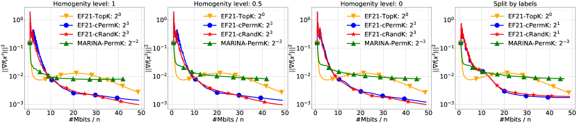
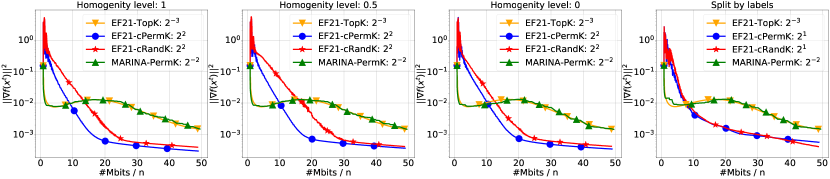
Number of clients $n=10$, compression level $K=2509$. Number of clients $n=100$, compression level $K=251$. Number of clients $n=1000$, compression level $K=25$.

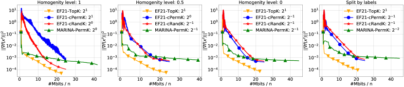
MARINA and greedy sparsification (3PCv5)

We now draw our attention to one of the newly proposed methods: MARINA combined with biased compression operators (named as 3PCv5 in Algorithm 9 and Table 1). According to our theory, see Table 1, 3PCv5 has the same compexity as EF21. In this experiment, we aim to validate the proposed method with greedy Top-$K$ sparsifier. We compare it to MARINA with Perm-$K$ and Rand-$K$ and include EF21 as a reference method. Interestingly, Top-$K$ improves over Perm-$K$ and Rand-$K$ when $n=10$; in homogeneus case, the behavior of Top-$K$ and Perm-$K$ is similar, see Figure 4. However, this improvement vanishes when $n$ is increased ($n=100,1000$) and sparsification is more agressive; MARINA with Top-$K$ requires much smaller step-sizes to converge. In all cases, EF21 with Top-$K$ is faster.

Figure 4: Comparison of MARINA with Perm-$K$, Rand-$K$ and 3PCv5 with Top-$K$.

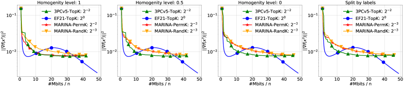
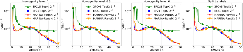
Number of clients $n=10$, compression level $K=2509$. Number of clients $n=100$, compression level $K=251$. Number of clients $n=1000$, compression level $K=25$.

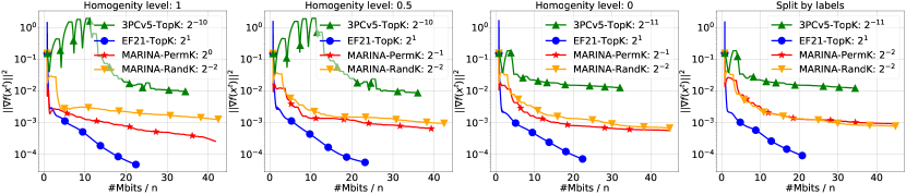
Other 3PC variants

Motivated by the success of greedy sparsification and favorable properties of randomized sparsifiers, we aim to investigate if one can combine the two in a nontrivial way and obtain even faster method. One possible way to do so is to look more closely to one of the special cases of 3PC named 3PCv2. With 3PCv2 (Algorithm 6), we have more freedom because it has two compressors. In our experiments, we consider three different sparsifiers (Top-$K$, Rand-$K$, Perm-$K$) as for the first compressor and fix the second one as Top-$K$, see Figure 5.

For $n=10$, the performance of 3PCv2 with Rand-$K$-Top-$K$ and Top-$K$-Top-$K$ is very similar to the one of EF21 with Top-$K$. Interestingly, 3PCv2-Rand-$K$-Top-$K$ becomes superior for $n=100$ converging even faster than EF21. The difference is especially prominent in heterogeneous setting. Finally, EF21 shows slightly beter performance in the experiments with $1000$ nodes. We can conclude that:

• 3PCv2 can outperform EF21 in some cases, for example, Figure 5,

• EF21 is still superior when $n$ is large.

However, more emprirical evidence is needed to investigate the behavior of 3PCv2 and other new methods fitting 3PC framework.

Figure 5: Comparison of 3PCv2 with Perm-$K$, Rand-$K$ and Top-$K$ as the first compressor. Top-$K$ is used as the second compressor. EF21 with Top-$K$ is provided for the reference.

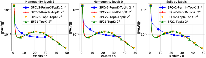
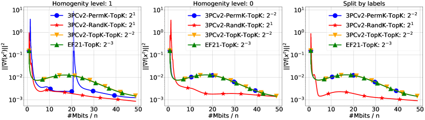
Number of clients $n=10$, compression level $K=2509$. Number of clients $n=100$, compression level $K=251$. Number of clients $n=100$, compression level $K=25$.

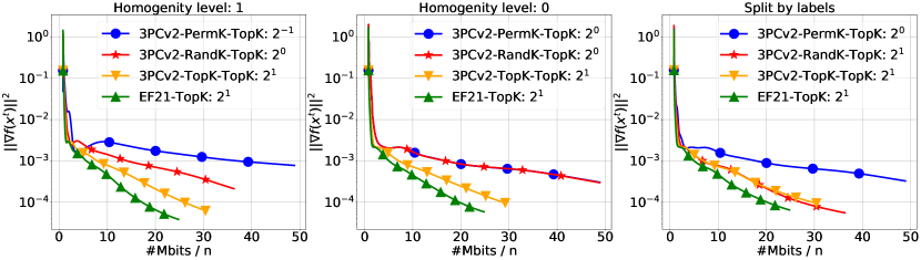
E.2 Solving synthetic quadratic problem

In this experimental section we compare practical performance of the proposed methods 3PCv1, 3PCv2, 3PCv4, 3PCv5 against existing state-of-the-art methods for compressed distributed optimization MARINA and EF21. For this comparison we set up the similar setting that was introduced in Szlendak et al. (2021). Firstly, let us describe the experimental setup in detail. We consider the finite sum function $f(x)=\frac{1}{n}\sum_{i=1}^{n}f_{i}(x)$, consisting of synthetic quadratic functions

$$f_{i}(x)=\frac{1}{2}x^{\top}\mathbf{A}_{i}x-x^{\top}b_{i},$$ (78)

where $\mathbf{A}_{i}\in\mathbb{R}^{d\times d}$, $b_{i}\in\mathbb{R}^{d},$ and $\mathbf{A}_{i}=\mathbf{A}_{i}^{\top}$ is the training data that belongs to the device/worker $i$. In all experiments of this section, we have $d=1000$ and generated $\mathbf{A}_{i}$ in a such way that $f$ is $\lambda$–strongly convex ( i.e., $\frac{1}{n}\sum_{i=1}^{n}\mathbf{A}_{i}\succcurlyeq\lambda\mathbf{I}$ for $\lambda>0$) with $\lambda=1\mathrm{e}^{-6}$. We now present Algorithm 11 which is used to generate these synthetic matrices (training data).

Algorithm 11 Quadratic optimization task generation (Szlendak et al., 2021)

1:  Parameters: number nodes $n$, dimension $d$, regularizer $\lambda$, and noise scale $s$.

2:  for $i=1,\dots,n$ do

3:     Generate random noises $\nu_{i}^{s}=1+s\xi_{i}^{s}$ and $\nu_{i}^{b}=s\xi_{i}^{b},$ i.i.d. $\xi_{i}^{s},\xi_{i}^{b}\sim\mathcal{N}(0,1)$

4:     Take vector $b_{i}=\frac{\nu_{i}^{s}}{4}(-1+\nu_{i}^{b},0,\cdots,0)\in\mathbb{R}^{d}$

5:     Take the initial tridiagonal matrix

$$\mathbf{A}_{i}=\frac{\nu_{i}^{s}}{4}\left(\begin{array}[]{cccc}2&-1&&0\\ -1&\ddots&\ddots&\\ &\ddots&\ddots&-1\\ 0&&-1&2\end{array}\right)\in\mathbb{R}^{d\times d}$$

6:  end for

7:  Take the mean of matrices $\mathbf{A}=\frac{1}{n}\sum_{i=1}^{n}\mathbf{A}_{i}$

8:  Find the minimum eigenvalue $\lambda_{\min}(\mathbf{A})$

9:  for $i=1,\dots,n$ do

10:     Update matrix $\mathbf{A}_{i}=\mathbf{A}_{i}+(\lambda-\lambda_{\min}(\mathbf{A}))\mathbf{I}$

11:  end for

12:  Take starting point $x^{0}=(\sqrt{d},0,\cdots,0)$

13:  Output: matrices $\mathbf{A}_{1},\cdots,\mathbf{A}_{n}$, vectors $b_{1},\cdots,b_{n}$, starting point $x^{0}$

We generated optimization tasks having different number of nodes $n=\left\{10,100,1000\right\}$ and capturing various data-heterogeneity regimes that are controlled by so-called Hessian variance term:

Definition E.1 (Hessian variance (Szlendak et al., 2021)).

Let $L_{\pm}\geq 0$ be the smallest quantity such that

$$\textstyle\frac{1}{n}\sum\limits_{i=1}^{n}\left\|\nabla f_{i}(x)-\nabla f_{i}(y)\right\|^{2}-\left\|\nabla f(x)-\nabla f(y)\right\|^{2}\leq L^{2}_{\pm}\left\|x-y\right\|^{2},\quad\forall x,y\in\mathbb{R}^{d}.$$ (79)

We refer to the quantity $L_{\pm}^{2}$ by the name Hessian variance.

From the definition , it follows that the case of similar (or even identical) functions $f_{i}$ relates to the small (or even $0$) Hessian variance, whereas in the case of completely different $f_{i}$ (which relate to heterogeneous data regime) $L_{\pm}$ can be large.

In our experiments, homogeneity of each optimizations task is controlled by noise scale $s$ introduced in the Algorithm 11. Indeed, for the noise scale $s=0$, all matrices $\mathbf{A}_{i}$ are equal, whereas with the increase of the noise scale, functions become less “similar” and $L_{\pm}$ rises. We take noise scales $s\in\left\{0.0,0.05,0.8,1.6,6.4\right\}$. A summary of the $L_{\pm}$ and $L_{-}$ values corresponding to these noise scales is given in the Tables 3 and 4. For the considered quadratic problem $L_{\pm}$ can be analytically expressed as $L_{\pm}=\sqrt{\lambda_{\max}\left(\frac{1}{n}\sum_{i=1}^{n}\mathbf{A}_{i}^{2}-\left(\frac{1}{n}\sum_{i=1}^{n}\mathbf{A}_{i}\right)^{2}\right)}$.

Table 3: Summary of the Hessian variance terms $L_{\pm}$ for different number of nodes $n$ various noise scales $s$.

	$0$	$0.05$	$0.8$	$1.6$	$6.4$
$10$	$0$	$0.06$	$0.9$	$1.79$	$7.17$
$100$	$0$	$0.05$	$0.82$	$1.65$	$6.58$
$1000$	$0$	$0.05$	$0.81$	$1.62$	$6.48$

Table 4: Summary of the Hessian variance terms $L_{-}$ for different number of nodes $n$ various noise scales $s$.

	$0$	$0.05$	$0.8$	$1.6$	$6.4$
$10$	$1.0$	$1.02$	$1.35$	$1.7$	$3.82$
$100$	$1.0$	$1.0$	$0.97$	$0.94$	$0.77$
$1000$	$1.0$	$1.0$	$0.97$	$0.95$	$0.78$

For all algorithms, at each iteration we compute the squared norm of the exact/full gradient for comparison of the methods performance. We terminate our algorithms either if they reach the certain number of iterations or the following stopping criterion is satisfied: $\left\|\nabla f(x^{t})\right\|^{2}\leq 10^{-7}$.

In all experiments, the stepsize of each method is set to the largest theoreticaly possible stepsize multiplied by some constant multiplier which was individually tuned in all cases within powers of $2$ : $\left\{2,4,8,16,32,64,128,256,512,1024,2048,4096,8192,16384,32768\right\}$ .

EF21 and different compressors

Following the same order as in the section E.1 we start by comparing existing SOTA methods (MARINA with Perm-$K$ and EF21 with Top-$K$) against EF21 with cPerm-$K$ and cRand-$K$. In Figure 6, paramater $K=\nicefrac{{d}}{{n}}$ is fixed for each row. Each column corresponds to a heterogeneity levels defined by the averaged $L_{\pm}$ and $L_{-}$ per values $n$ (averaged per column in the Tables 3 and 4).

Figure 6: Comparison of MARINA with Perm-$K$, EF21 with Top-$K$, cPerm-$K$ and cRand-$K$ with $K=\nicefrac{{d}}{{n}}$ and tuned stepsizes. By $1\times,2\times,4\times$ (and so on) we indicate that the stepsize is set to a multiple of the largest stepsize predicted by theory. $L_{\pm}^{avg}$ and $L_{-}^{avg}$ are the averaged constants $L_{\pm}$ and $L_{-}$ per column.

These experiments shows that, in low Hessian variance regime EF21 with cPerm-$K$ and cRand-$K$ in some cases improves MARINA with Perm-$K$ for $n=10,100$, whereas for $n=1000$ MARINA with cPerm-$K$ still dominates. Moreover, even in big Hessian variance regime ${\sf\color[rgb]{0.15234375,0.51171875,0.26171875}EF21}$ methods converges faster than MARINA with cPerm-$K$ but not as fast as EF21 with Top-$K$. We are not aware of any prior empirical study for EF21 combined with cPerm-$K$ or cRand-$K$.

MARINA and different compressors

In this section, we keep the same setting and compare a new method 3PCv5 with Top-$K$ against MARINA with Perm-$K$, Rand-$K$ and EF21 with Top-$K$. In Figure 7, one can see that 3PCv5 with Top-$K$ outperforms MARINA methods only in a couple of cases for $n=10$, whereas for the most of the regimes it converges slower than other methods.

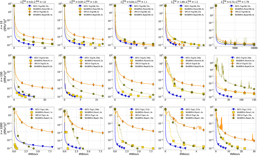
Figure 7: Comparison of MARINA with Perm-$K$, Rand-$K$, EF21 with Top-$K$ and 3PCv5 with $K=\nicefrac{{d}}{{n}}$ and tuned stepsizes. By $1\times,2\times,4\times$ (and so on) we indicate that the stepsize is set to a multiple of the largest stepsize predicted by theory. $L_{\pm}^{avg}$ and $L_{-}^{avg}$ are the averaged constants $L_{\pm}$ and $L_{-}$ per column.

3PCv2 beat SOTA methods in the most cases!

In this series of experiments, we stick to the previous setting and append the results of the new method 3PCv2 with 2 different combinataion of compressors: Rand$K_{1}$-Top$K_{2}$ and Rand$K_{1}$ $*$Perm$K$ -Top$K_{2}$, where Rand$K_{1}$ $*$Perm-$K$ is the composition of Rand-$K_{1}$ and Perm-$K$. For both methods, constants $K_{1}$ and $K_{2}$ were extensively tuned over the set of $9$ different pairs (see Figures 10 and 12 for details). In the Figure 8 it is shown that both variants 3PCv2 methods converge quickly for $n=100$ in all heterogeneity regimes, outperforming MARINA and EF21. In the big Hessian variance regime and $n=10$, 3PCv2 also converges faster than EF21 with Top-$K$, however, for even more homogeneous cases 3PCv2 slightly looses to EF21 with cPerm-$K$ or cRand-$K$. We also would like to note that we excluded 3PCv4 with Top$K_{1}$-Top$K_{2}$ from our comparison here since in practice for $K=\nicefrac{{d}}{{n}}$ it coincides with EF21 with Top-$K$ (see Figure 14 for more details)

Figure 8: Comparison of MARINA, EF21, 3PCv2 and 3PCv5 with various compressors , $K=\nicefrac{{d}}{{n}}$ and tuned stepsizes. By $1\times,2\times,4\times$ (and so on) we indicate that the stepsize is set to a multiple of the largest stepsize predicted by theory. $L_{\pm}^{avg}$ and $L_{-}^{avg}$ are the averaged constants $L_{\pm}$ and $L_{-}$ per column.

We further continue with the setting where $\nicefrac{{K}}{{d}}=0.02$ is fixed for each $n$. In the Figure 9 illustrates that 3PCv2 remaines the best choice for $n=10$ and $n=100$, whereas in the homogeneous regime and $n=1000$ EF21 with cRand-$K$ can reach the desired tolerance a bit faster. However, for big Hessian varince regime 3PCv2 as again preferable.

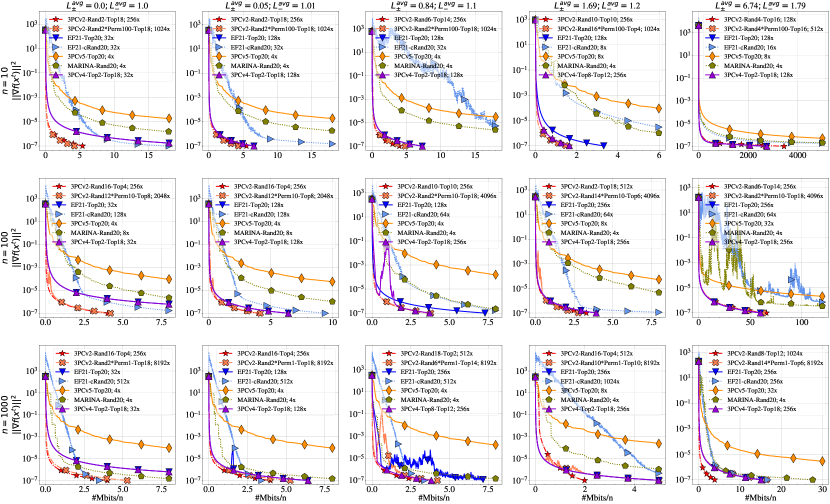
Figure 9: Comparison of MARINA, EF21, 3PCv2, 3PCv5 and 3PCv5 with various compressors , $K=0.02{d}$ and tuned stepsizes. By $1\times,2\times,4\times$ (and so on) we indicate that the stepsize is set to a multiple of the largest stepsize predicted by theory. $L_{\pm}^{avg}$ and $L_{-}^{avg}$ are the averaged constants $L_{\pm}$ and $L_{-}$ per column.

Fine-tuning of $(K_{1},K_{2})$ pairs for 3PCv2 and 3PCv4

In this section we provide with some auxillary results on the demonstration of the tuning $(K_{1},K_{2})$ pairs for 3PCv2 and 3PCv4 on different compressors. In the $K=\nicefrac{{d}}{{n}}$ scenario (see Figure 10), in all cases the best performance of 3PCv2 with Rand$K_{1}$-Top$K_{2}$ is achieved when $K_{2}>K_{1}$, whereas for the case when $\nicefrac{{K}}{{d}}=0.02$ (see Figure 11) there is a dependence on $n$; for $n=10$, the choice when $K_{2}>K_{1}$ is preferable in all cases, whereas for $n=100$ and $n=1000$ it is the case only in big Hessian variance regime. At the same time, for optimal pairs $(K_{1},K_{2})$ of the method 3PCv2 with Rand$K_{1}*$Perm$K$-Top$K_{2}$ we observe that the choice is $K_{2}>K_{1}$ (see Figures 12, 13).

Figure 10: Comparison of 3PCv2 with methods with Rand$K_{1}$-Top$K_{2}$ with $K_{1}+K_{2}=\nicefrac{{d}}{{n}}$ and tuned stepsizes. By $1\times,2\times,4\times$ (and so on) we indicate that the stepsize is set to a multiple of the largest stepsize predicted by theory. $L_{\pm}^{avg}$ and $L_{-}^{avg}$ are the averaged constants $L_{\pm}$ and $L_{-}$ per column.

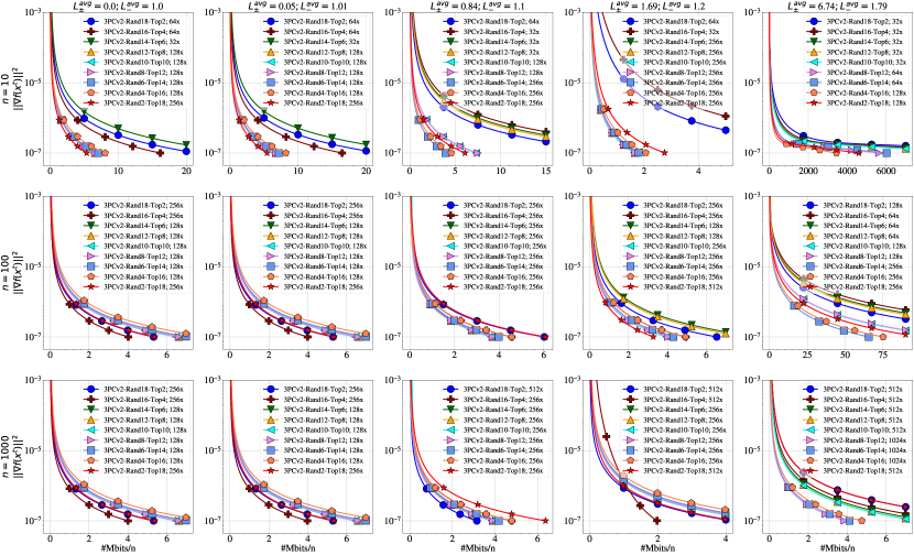
Figure 11: Comparison of 3PCv2 with methods with Rand$K_{1}$-Top$K_{2}$ with $K_{1}+K_{2}=0.02{d}$ and tuned stepsizes. By $1\times,2\times,4\times$ (and so on) we indicate that the stepsize is set to a multiple of the largest stepsize predicted by theory. $L_{\pm}^{avg}$ and $L_{-}^{avg}$ are the averaged constants $L_{\pm}$ and $L_{-}$ per column.

Figure 12: Comparison of 3PCv2 with methods with Rand$K_{1}*$Perm$K$-Top$K_{2}$ with $K_{1}+K_{2}=\nicefrac{{d}}{{n}}$ and tuned stepsizes. By $1\times,2\times,4\times$ (and so on) we indicate that the stepsize is set to a multiple of the largest stepsize predicted by theory. $L_{\pm}^{avg}$ and $L_{-}^{avg}$ are the averaged constants $L_{\pm}$ and $L_{-}$ per column.

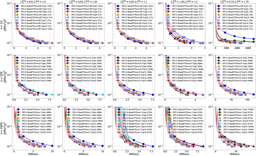
Figure 13: Comparison of 3PCv2 with methods with Rand$K_{1}*$Perm$K$-Top$K_{2}$ with $K_{1}+K_{2}=0.02{d}$ and tuned stepsizes. By $1\times,2\times,4\times$ (and so on) we indicate that the stepsize is set to a multiple of the largest stepsize predicted by theory. $L_{\pm}^{avg}$ and $L_{-}^{avg}$ are the averaged constants $L_{\pm}$ and $L_{-}$ per column.

Figures 14 and 15 show that for the considered sparse quadratic problem in most cases the method 3PCv4 with Top$K_{1}$-Top$K_{2}$ compressors behaves as a EF21 with Top-$K$. Only in a few cases 3PCv4 shows an improvement over EF21.

Figure 14: Comparison of 3PCv4 with methods with Top$K_{1}$-Top$K_{2}$ with $K_{1}+K_{2}=\nicefrac{{d}}{{n}}$ and tuned stepsizes. By $1\times,2\times,4\times$ (and so on) we indicate that the stepsize is set to a multiple of the largest stepsize predicted by theory. $L_{\pm}^{avg}$ and $L_{-}^{avg}$ are the averaged constants $L_{\pm}$ and $L_{-}$ per column.

Figure 15: Comparison of 3PCv4 with methods with Top$K_{1}$-Top$K_{2}$ with $K_{1}+K_{2}=0.02{d}$ and tuned stepsizes. By $1\times,2\times,4\times$ (and so on) we indicate that the stepsize is set to a multiple of the largest stepsize predicted by theory. $L_{\pm}^{avg}$ and $L_{-}^{avg}$ are the averaged constants $L_{\pm}$ and $L_{-}$ per column.

3PCv1

The next sequence of plots compares EF21 with Top-$K$, 3PCv1 with Top-$K$ and classical GD. Since all methods communicates different amount of floats on each iteration they are compared in terms of the # communication rounds. Yet being unpractical, 3PCv1 can provide an intuition of how the intermediate method between GD and EF21 could work and what performance can be achieved in 3PCv1 by additional sending $d$ dimensional vector from each node to the server. Figure 16 illustrates that in low Hessian variance regime 3PCv1 with Top-$K$ behaves as a classical GD, whereas in a more heterogeneous regime, it can loose GD in terms of the number of communication rounds.

Figure 16: Comparison of GD , 3PCv1 with Top-$K$ and EF21 with Top-$K$ for $K=0.02{d}$ and tuned stepsizes. By $1\times,2\times,4\times$ (and so on) we indicate that the stepsize is set to a multiple of the largest stepsize predicted by theory. $L_{\pm}^{avg}$ and $L_{-}^{avg}$ are the averaged constants $L_{\pm}$ and $L_{-}$ per column.

E.3 Testing compressed lazy aggregation (CLAG)

Following  Richtárik et al. (2021), we show the performance advantages of CLAG. We recall that we are interested in solving the non-convex logistic regression problem,

$$\min\limits_{x\in\mathbb{R}^{d}}f(x)=\frac{1}{N}\sum\limits_{i=1}^{N}\log(1+\exp(-y_{i}a_{i}^{\top}x))+\lambda\sum\limits_{j=1}^{d}\frac{x_{j}^{2}}{1+x_{j}^{2}},$$ (80)

where $a_{i}\in\mathbb{R}^{d},y_{i}\in\{-1,1\}$ are the training data, and $\lambda>0$ is a regularization parameter. Parameter $\lambda$ is always set to $0.1$ in the experiments. We use four LIBSVM Chang & Lin (2011) datasets phishing, w6a, a9a, ijcnn1 as training data. A dataset has been evenly split into $n=20$ equal parts where each part represents a separate client dataset (the remainder of partition between clients has been withdrawn).

Heatmap of communication complexities of CLAG for different combinations of parameters. In our first group of experiments (see Figures 17, 18, 19, 20), we run CLAG with Top-$K$ compressor. The compression level $K$ varies evenly between $1$ and $d$, where $d$ is the number of features of a chosen dataset. Trigger $\zeta$ passes zero and subsequent powers of two from zero to eleven. For each combination of $K$ and $\zeta$, we compute empirically the minimum number of bits per worker sent from clients to the server. Minimum is taken among 12 launches of CLAG with different scalings of the theoretical stepsize, scales are powers of two from zero to eleven. The stopping criterion for each launch is based on the condition: $\|\nabla f(x)\|<\delta$, where $\delta$ equals to $10^{-4}$ for phishing and to $10^{-2}$ for a9a, ijcnn1 and w6a datasets. Since the algorithm may not converge with too large stepsizes, the time limit of five minutes has been set for one launch. We stress that CLAG reduces to LAG when $k=d$ and to EF21 when $\zeta=0$. The experiment shows that for the most of datasets (excluding phishing) the minimum communication complexity is attained at a combination of $(K,\zeta)$, which does not reduce CLAG to EF21 or LAG. Thus CLAG can be consistently faster than EF21 and LAG.

Plots for limited communication cost. In our second group of experiments (see Figures  21, 22, 23, 24), we are in the same setup as in the previous one but this time the stopping criterion bounds the communication cost of algorithms; CLAG, LAG and EF21 stop when they first hit the communication cost of 32 Mbits per client. Compression levels $K$ for each dataset at each plot correspond to $1$, $25\%$ and $50\%$ of features. Stepsizes for each algorithm is fine-tuned over the same grid as in the previous experiment. The best $\zeta$ are chosen for CLAG and LAG from the same grid as in the previous experiment. The experiment exhibits again but from the different perspective the advantages of CLAG over its counterparts.

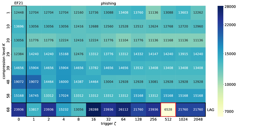
Figure 17: Heatmap of communication complexities of CLAG for different combination of compression levels and triggers with fine-tuned stepsizes on phishing dataset. We contour cells corresponding to EF21 and LAG, as special cases of CLAG, by black rectangles. The red-countered cell indicates the experiment with the smallest communication cost.

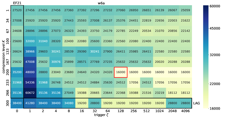
Figure 18: Heatmap of communication complexities of CLAG for different combination of compression levels and triggers with fine-tuned stepsizes on w6a dataset. We contour cells corresponding to EF21 and LAG, as special cases of CLAG, by black rectangles. The red-countered cell indicates the experiment with the smallest communication cost.

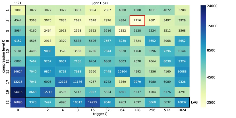
Figure 19: Heatmap of communication complexities of CLAG for different combination of compression levels and triggers with fine-tuned stepsizes on ijcnn1 dataset. We contour cells corresponding to EF21 and LAG, as special cases of CLAG, by black rectangles. The red-countered cell indicates the experiment with the smallest communication cost.

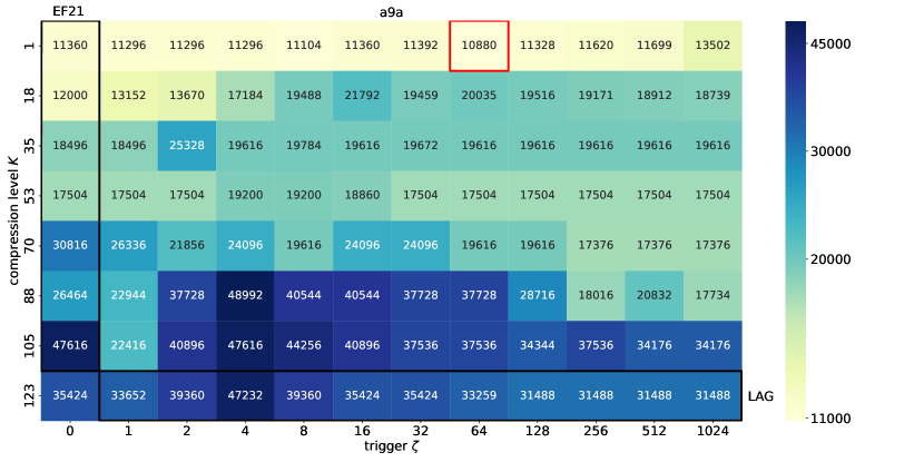
Figure 20: Heatmap of communication complexities of CLAG for different combination of compression levels and triggers with fine-tuned stepsizes on a9a dataset. We contour cells corresponding to EF21 and LAG, as special cases of CLAG, by black rectangles. The red-countered cell indicates the experiment with the smallest communication cost.We contour cells corresponding to EF21 and LAG, as special cases of CLAG, by black rectangles. The red-countered cell indicates the experiment with the smallest communication cost.

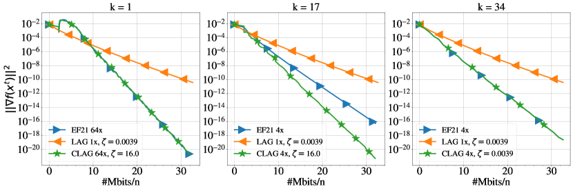
Figure 21: Comparison of CLAG, LAG and EF21 with Top-$K$ with fine-tuned stepsizes on phishing dataset

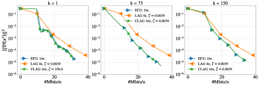
Figure 22: Comparison of CLAG, LAG and EF21 with Top-$K$ with fine-tuned stepsizes on w6a dataset

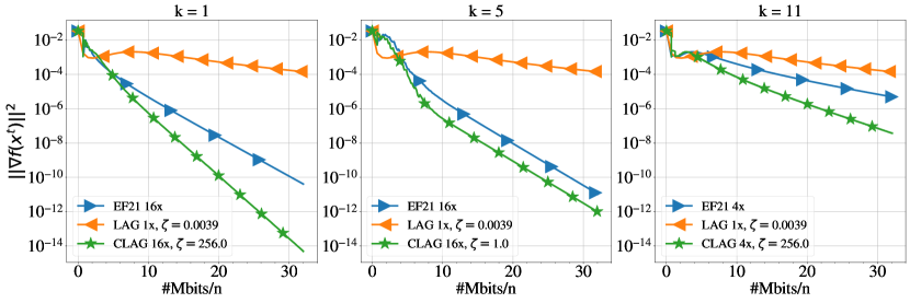
Figure 23: Comparison of CLAG, LAG and EF21 with Top-$K$ with fine-tuned stepsizes on ijcnn1 dataset

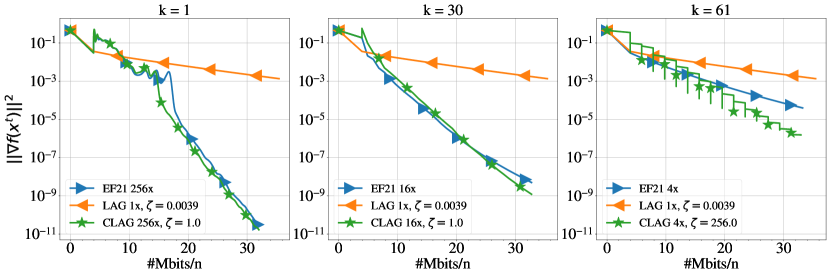
Figure 24: Comparison of CLAG, LAG and EF21 with Top-$K$ with fine-tuned stepsizes on a9a dataset

References

- Alistarh et al. (2018) Alistarh, D., Hoefler, T., Johansson, M., Khirirat, S., Konstantinov, N., and Renggli, C. The convergence of sparsified gradient methods. In Advances in Neural Information Processing Systems (NeurIPS), 2018.
- Beznosikov et al. (2020) Beznosikov, A., Horváth, S., Richtárik, P., and Safaryan, M. On biased compression for distributed learning. arXiv preprint arXiv:2002.12410, 2020.
- Bottou (2012) Bottou, L. Stochastic Gradient Descent Tricks, volume 7700 of Lecture Notes in Computer Science (LNCS), pp. 430–445. Springer, neural networks, tricks of the trade, reloaded edition, January 2012. URL https://www.microsoft.com/en-us/research/publication/stochastic-gradient-tricks/.
- Chang & Lin (2011) Chang, C.-C. and Lin, C.-J. LIBSVM: a library for support vector machines. ACM Transactions on Intelligent Systems and Technology (TIST), 2(3):1–27, 2011.
- Chen et al. (2018) Chen, T., Giannakis, G., Sun, T., and Yin, W. LAG: Lazily aggregated gradient for communication-efficient distributed learning. Advances in Neural Information Processing Systems, 2018.
- Dean et al. (2012) Dean, J., Corrado, G., Monga, R., Chen, K., Devin, M., Mao, M., Senior, A., Tucker, P., Yang, K., Le, Q. V., and et al. Large scale distributed deep networks. In Advances in Neural Information Processing Systems, pp. 1223–1231, 2012.
- Fatkhullin et al. (2021) Fatkhullin, I., Sokolov, I., Gorbunov, E., Li, Z., and Richtárik, P. Ef21 with bells & whistles: practical algorithmic extensions of modern error feedback. arXiv preprint arXiv:2110.03294, 2021.
- Ghadikolaei et al. (2021) Ghadikolaei, H. S., Stich, S., and Jaggi, M. LENA: Communication-efficient distributed learning with self-triggered gradient uploads. In International Conference on Artificial Intelligence and Statistics, pp. 3943–3951. PMLR, 2021.
- Gorbunov et al. (2020) Gorbunov, E., Kovalev, D., Makarenko, D., and Richtárik, P. Linearly converging error compensated SGD. In 34th Conference on Neural Information Processing Systems (NeurIPS), 2020.
- Gorbunov et al. (2021) Gorbunov, E., Burlachenko, K. P., Li, Z., and Richtárik, P. MARINA: Faster non-convex distributed learning with compression. In Meila, M. and Zhang, T. (eds.), Proceedings of the 38th International Conference on Machine Learning, volume 139 of Proceedings of Machine Learning Research, pp. 3788–3798. PMLR, 18–24 Jul 2021. URL https://proceedings.mlr.press/v139/gorbunov21a.html.
- Horváth & Richtárik (2020) Horváth, S. and Richtárik, P. A better alternative to error feedback for communication-efficient distributed learning. arXiv preprint arXiv:2006.11077, 2020.
- Horváth & Richtárik (2021) Horváth, S. and Richtárik, P. A better alternative to error feedback for communication-efficient distributed learning. In 9th International Conference on Learning Representations (ICLR), 2021.
- Karimireddy et al. (2019) Karimireddy, S. P., Rebjock, Q., Stich, S., and Jaggi, M. Error feedback fixes SignSGD and other gradient compression schemes. In 36th International Conference on Machine Learning (ICML), 2019.
- Khaled et al. (2020) Khaled, A., Mishchenko, K., and Richtárik, P. Tighter theory for local SGD on identical and heterogeneous data. In The 23rd International Conference on Artificial Intelligence and Statistics (AISTATS 2020), 2020.
- Khirirat et al. (2018) Khirirat, S., Feyzmahdavian, H. R., and Johansson, M. Distributed learning with compressed gradients. arXiv preprint arXiv:1806.06573, 2018.
- Kingma & Ba (2014) Kingma, D. P. and Ba, J. Adam: a method for stochastic optimization. In The 3rd International Conference on Learning Representations, 2014. URL https://arxiv.org/pdf/1412.6980.pdf.
- Koloskova et al. (2020) Koloskova, A., Lin, T., Stich, S., and Jaggi, M. Decentralized deep learning with arbitrary communication compression. In International Conference on Learning Representations (ICLR), 2020.
- Konečný et al. (2016a) Konečný, J., McMahan, H. B., Ramage, D., and Richtárik, P. Federated optimization: distributed machine learning for on-device intelligence. arXiv:1610.02527, 2016a.
- Konečný et al. (2016b) Konečný, J., McMahan, H. B., Yu, F., Richtárik, P., Suresh, A. T., and Bacon, D. Federated learning: strategies for improving communication efficiency. In NIPS Private Multi-Party Machine Learning Workshop, 2016b.
- LeCun et al. (2010) LeCun, Y., Cortes, C., and Burges, C. Mnist handwritten digit database. ATTLabs [Online], 2010. URL http://yann.lecun.com/exdb/mnist.
- Li & Richtárik (2020) Li, Z. and Richtárik, P. A unified analysis of stochastic gradient methods for nonconvex federated optimization. arXiv preprint arXiv:2006.07013, 2020.
- Li & Richtárik (2021) Li, Z. and Richtárik, P. CANITA: Faster rates for distributed convex optimization with communication compression. In Advances in Neural Information Processing Systems, 2021. arXiv:2107.09461.
- Li et al. (2020) Li, Z., Kovalev, D., Qian, X., and Richtárik, P. Acceleration for compressed gradient descent in distributed and federated optimization. In International Conference on Machine Learning (ICML), pp. 5895–5904. PMLR, 2020.
- Li et al. (2021) Li, Z., Bao, H., Zhang, X., and Richtárik, P. PAGE: A simple and optimal probabilistic gradient estimator for nonconvex optimization. In International Conference on Machine Learning (ICML), pp. 6286–6295. PMLR, 2021.
- Lin et al. (2018) Lin, Y., Han, S., Mao, H., Wang, Y., and Dally, B. Deep gradient compression: Reducing the communication bandwidth for distributed training. In International Conference on Learning Representations, 2018.
- McMahan et al. (2016) McMahan, B., Moore, E., Ramage, D., and Agüera y Arcas, B. Federated learning of deep networks using model averaging. arXiv preprint arXiv:1602.05629, 2016.
- McMahan et al. (2017) McMahan, H. B., Moore, E., Ramage, D., Hampson, S., and Agüera y Arcas, B. Communication-efficient learning of deep networks from decentralized data. In Proceedings of the 20th International Conference on Artificial Intelligence and Statistics (AISTATS), 2017.
- Mishchenko et al. (2019) Mishchenko, K., Gorbunov, E., Takáč, M., and Richtárik, P. Distributed learning with compressed gradient differences. arXiv preprint arXiv:1901.09269, 2019.
- Nesterov et al. (2018) Nesterov, Y. et al. Lectures on convex optimization, volume 137. Springer, 2018.
- Richtárik et al. (2021) Richtárik, P., Sokolov, I., and Fatkhullin, I. EF21: A new, simpler, theoretically better, and practically faster error feedback. In Advances in Neural Information Processing Systems, 2021.
- Safaryan et al. (2021a) Safaryan, M., Islamov, R., Qian, X., and Richtárik, P. FedNL: Making Newton-type methods applicable to federated learning. arXiv preprint arXiv:2106.02969, 2021a.
- Safaryan et al. (2021b) Safaryan, M., Shulgin, E., and Richtárik, P. Uncertainty principle for communication compression in distributed and federated learning and the search for an optimal compressor. Information and Inference: A Journal of the IMA, 2021b.
- Seide et al. (2014) Seide, F., Fu, H., Droppo, J., Li, G., and Yu, D. 1-bit stochastic gradient descent and its application to data-parallel distributed training of speech DNNs. In Fifteenth Annual Conference of the International Speech Communication Association, 2014.
- Stich (2020) Stich, S. U. Local SGD converges fast and communicates little. In International Conference on Learning Representations, 2020.
- Stich et al. (2018) Stich, S. U., Cordonnier, J.-B., and Jaggi, M. Sparsified SGD with memory. In Advances in Neural Information Processing Systems (NeurIPS), 2018.
- Sun et al. (2019) Sun, J., Chen, T., Giannakis, G., and Yang, Z. Communication-efficient distributed learning via lazily aggregated quantized gradients. Advances in Neural Information Processing Systems, 32:3370–3380, 2019.
- Szlendak et al. (2021) Szlendak, R., Tyurin, A., and Richtárik, P. Permutation compressors for provably faster distributed nonconvex optimization. arXiv preprint arXiv:2110.03300, 2021, 2021.
- Tang et al. (2020) Tang, H., Lian, X., Yu, C., Zhang, T., and Liu, J. DoubleSqueeze: Parallel stochastic gradient descent with double-pass error-compensated compression. In Proceedings of the 36th International Conference on Machine Learning (ICML), 2020.
- Woodworth et al. (2020) Woodworth, B., Patel, K. K., Stich, S. U., Dai, Z., Bullins, B., McMahan, H. B., Shamir, O., and Srebro, N. Is local SGD better than minibatch SGD? arXiv preprint arXiv:2002.07839, 2020.