The spatial distribution of globular clusters in dwarf spheroidal galaxies and the timing problem

Abstract

The dynamical friction timescale of massive globular clusters (GCs) in the inner regions of cuspy dark haloes in dwarf spheroidal (dSph) galaxies can be much shorter than the Hubble time. This implies that a small fraction of the GCs is expected to be caught close to the centre of these galaxies. We compare the radial distribution of GCs predicted in simple Monte Carlo models with that of a sample of $38$ spectroscopically confirmed GCs plus $17$ GC candidates, associated mainly to low-luminosity dSph galaxies. If dark matter haloes follow an NFW profile, the observed number of off-center GCs at projected distances less than one half the galaxy effective radius is significantly higher than models predict. This timing problem can be viewed as a fine-tuning of the starting GC distances. As a result of the short sinking timescale for GCs in the central regions, the radial distribution of GCs is expected to evolve significantly during the next $1-2$ Gyr. However, dark matter haloes with cores of size comparable to the galaxy effective radii can lead to a slow orbital in-spiral of GCs in the central regions of these galaxies, providing a simple solution to the timing problem. We also examine any indication of mass segregation in the summed distribution of our sample of GCs.

1 Introduction

Globular clusters (GCs) are believed to have formed within the high-pressure environments of the protogalaxies or during mergers of galaxies (Elmegreen & Efremov, 1997; Kruijssen, 2012, 2014; Lahén et al., 2019). In massive early-type galaxies, GCs are found to display a colour bimodality: red (metal-rich) and blue (metal-poor) GCs. The metal-rich GCs approximatelly follow the galaxy stellar surface brightness profile, while the blue, metal-poor GCs have typically a more extended spatial distribution. This may indicate that metal-poor GCs were formed at early stages of galaxy formation, or they were accreted onto the host galaxy from tidally stripped dwarf satellite galaxies (e.g., Forbes & Remus, 2018).

Some authors have pointed out that the radial distribution of GCs in elliptical galaxies, being less centrally concentrated than the halo stars, may be a consequence of the combination of different evolutionary processes, such as dynamical friction and tidal dissolution (e.g., Capuzzo-Dolcetta & Tesseri, 1999; Capuzzo-Dolcetta & Donnarumma, 2001). The fusion of GCs that sink into the central regions may lead to the formation of nuclear star clusters (NSCs) as those observed in many intermediate-mass galaxies, including the Milky Way (Capuzzo-Dolcetta & Miocchi, 2008; Antonini et al., 2012; Gnedin et al., 2014), and in low-mass early-type galaxies (e.g., Tremaine et al., 1975; Lotz et al., 2001). For galaxies with absolute magnitudes in the range $-19\leq M_{B}\leq-12$, the scaling relation between the luminosity of the host galaxy and the luminosity of the NSC is consistent with the GC merging scenario (Turner et al., 2012; den Brok et al., 2014; Carlsten et al., 2021).

For a sample of dwarf galaxies containing $30$ dwarf irregular galaxies (dIrr), $2$ dE, $2$ dwarf spheroidal (dSph) galaxies and $2$ Magellanic spirals (Sm galaxies), Georgiev et al. (2009) find that the most luminous GCs tend to be more centrally located (see also Tudorica et al., 2015). They argue that this luminosity segregation could be the result of the combined effect of dynamical friction plus a preference for the formation of more massive GCs in the nuclear regions.

The radial migration of GCs in dSph and dIrr galaxies could provide clues on the dark matter density profile in these galaxies and about the mechanisms for building up NSCs (e.g., Leaman et al., 2020). While the rotation curves of dwarf galaxies favour dark matter haloes with a constant-density core, determinations of the value of the inner slope of the dark matter profile from the stellar kinematics in pressure-supported dwarf galaxies is a delicate issue. Many investigations have modelled the stellar kinematics of the classical Milky Way dSph galaxies to infer their dark matter distribution. Most of the studies favour a cuspy dark matter inner profile for Draco (Jardel & Gebhardt, 2013; Jardel et al., 2013; Read et al., 2018, 2019; Hayashi et al., 2020; Massari et al., 2020), but a cored halo for Fornax (Walker & Peñarrubia, 2011; Amorisco & Evans, 2012; Pascale et al., 2018; Read et al., 2019). In the case of Sculptor, the results have been conflicting; some favour a cuspy halo (Richardson & Fairbairn, 2014; Massari et al., 2018), some favour a cored halo (e.g., Walker & Peñarrubia, 2011), and other conclude that both are consistent with observations (e.g., Strigari et al., 2018; Genina et al., 2018). According to the models in Hayashi et al. (2020), the classical dSph galaxies favour cuspy dark matter inner profiles, $\rho\propto r^{-\gamma}$, with $\gamma$ between $0.4$ and $1.35$, albeit with large uncertainties (see also Read et al., 2019). A cored dark halo is consistent with the available kinematic data in the case of Sextans, Sculptor and Fornax, within $95$ percent confidence intervals.

Much effort has been devoted to place constraints on the dark matter density distribution of Fornax dSph galaxy from the present-day distribution of its GCs (Tremaine, 1976; Goerdt et al., 2006; Sánchez-Salcedo et al., 2006; Angus & Diaferio, 2009; Inoue, 2009; Cole et al., 2012; Arca-Sedda & Capuzzo-Dolcetta, 2016; Boldrini et al., 2019; Leung et al., 2020; Meadows et al., 2020; Bar et al., 2021; Shao et al., 2021). A cored dark matter halo could explain the so-called timing problem, that is, why none of the five GCs in Fornax dSph galaxy have been sunk to the centre if the dynamical friction timescale, at least for two of them, is shorter than the age of the GCs. However, a cuspy halo cannot be ruled out. Cole et al. (2012) find that if the GCs were formed within the tidal radius of Fornax and the dark matter halo is cuspy, at least one GC is dragged to the centre in $1-2$ Gyr, except when selecting very particular initial conditions of the orbits ($\sim 2$ per cent probability). They suggest that the Fornax GCs could have been accreted via merger or tidal capture. On the other hand, Arca-Sedda & Capuzzo-Dolcetta (2016) find that the GCs could have been formed in situ in a cuspy halo if they are on circular orbits and their projected distances to the Fornax centre are close to the three-dimensional (3D) distances. Leung et al. (2020) use a different approach; they constrain the formation location of the GCs in Fornax, and argue that the present-day positions of the GCs require a large dark matter core and a dwarf-dwarf merger. Meadows et al. (2020) compare the GC in-spiralling rates in cuspy and cored dark haloes and conclude that the spatial distribution of GCs in Fornax cannot be used to distinguish between cored and cuspy potentials. In a recent work, Shao et al. (2021) suggest that the sinking timescale of the GCs in Fornax may be underestimated if the present-day mass of the dark matter halo derived from stellar kinematic analysis is used to compute it, because Fornax dSph galaxy may have undergone significant mass stripping. Even more remarkably, the present-day distribution of GCs found in the cosmological hydrodynamical simulation E-MOSAICS, which includes the formation and evolution of GCs, is fully consistent with that of Fornax (Shao et al., 2021).

As a further step towards understanding the role of dynamical friction and its effect on GCs orbiting dwarf galaxies, we investigate the spatial distribution of GCs in a sample of low-luminosity dwarf galaxies. Using a probabilistic approach, we explore if the main properties of the summed distribution of GCs in these galaxies can be accounted for, in a simple scenario where the orbits of the GCs decay towards the centres of galaxies due to dynamical friction with the dark matter particles in a cuspy halo or, on the contrary, it requires a finely tuned set of initial conditions.

The paper is organized as follows. In Section 2, we describe our sample of GCs. In Section 3, we search for any statistical correlation between relevant quantities. In particular, we investigate any evidence of mass segregation of GCs. In Section 4 we describe the input parameters of simple Monte Carlo models, which are used as a tool to interpret the present-day spatial distribution of GCs. In Section 5, we compare the expected radial distributions of GCs with the observed one, assuming that the dark matter haloes are cuspy. In Section 6 we study the past and future spatial distributions of the GCs in these haloes. In Section 7 we show that the distribution of GCs is consistent with cored dark matter haloes. There, we also discuss the limitations of our approach. Finally, our main conclusions are summarized in Section 8.

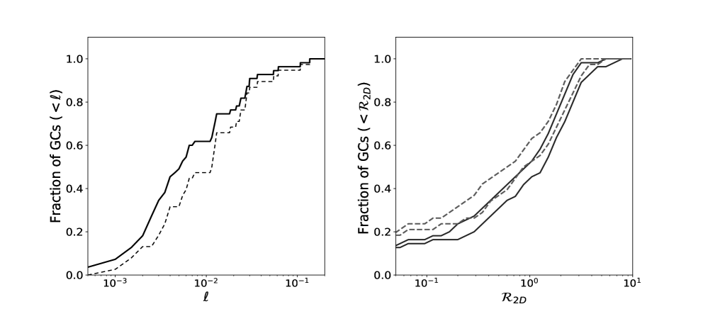
Figure 1: Cumulative distributions of the specific luminosity $\ell\equiv L_{\scriptscriptstyle V,\rm GC}/L_{\scriptscriptstyle V,\rm gal}$ (left panel) and the dimensionless projected radius $\mathcal{R}_{2\scriptscriptstyle\rm D}\equiv R_{\rm proj}/R_{e}$ (right panel) for the GCs in the extended sample (solid lines) and for confirmed GCs (dashed lines). In the right panel, the curves delineate the $2\sigma$ confidence bands.

Table 1: Fundamental parameters of galaxies

Name	Type	$D$	$M_{V}$	$R_{e}$	$\Theta$	Number of GCs	Source
		(Mpc)		$(\arcsec)$		Total (confirmed)
(1)	(2)	(3)	(4)	(5)	(6)	(7)	(8)
Fornax dSph	$-3$	0.147	$-13.30$	$996\pm 108$	$2.3$	5 (5)	M12, dB16
Eridanus II	$-3$	0.366	$-7.1$	$138.6\pm 7.2$	$1.5$	1 (1)	Cr16, S21
And I (KK 8)	$-3$	0.745	$-11.7$	$186\pm 19$	$3.7$	1 (0)	M12, Ca17
And XXV	$-3$	0.812	$-9.7$	$180\pm 15$	$3.0$	1 (1)	Cu16
DDO 216 (PegDIG)	$10^{\star}$	0.920	$-12.5$	$156\pm 8.5$	$1.2$	1 (1)	M12, K14, Co17
Sextans A (UGCA 205, DDO 75)	$10^{\ast}$	1.42	$-14.2$	$148\pm 14$	$-0.6$	1 (1)	M12, B14, B19
KKs 3	$-3$	2.12	$-12.3$	$50\pm 15$	$-0.3$	1 (1)	K15, S17
KKs 55	$-3$	3.94	$-11.17$	$50\pm 5$	$3.1$	1 (0)	K04, S08, G09
KKs 58	$-3^{\star}$	3.36	$-11.93$	$15.0\pm 0.5$	$0.6$	1 (1)	F20
Sc 22 (Scl-dE1)	$-3$	4.3	$-11.50$	$35\pm 10$	$0.9$	1 (1)	S08, D09
IKN	$-3$	3.61	$-11.5$	$55\pm 16$	$2.7$	5 (5)	T15
BK6N (KK 91)	$-3$	3.85	$-11.92$	$28\pm 12$	$1.1$	2 (0)	K04, S08, C09, S05
KK 27	$-3$	3.98	$-12.32$	$25\pm 2$	$1.3$	1 (0)	K04, S08, S05
KK 77	$-3$	3.48	$-12.21$	$34\pm 4$	$2.0$	3 (0)	K04, S08, C09, S05
KK 197	$-3^{\star}$	3.87	$-13.04$	$38\pm 11$	$3.0$	3 (3)	S08, G09, F20
KK 211	$-5$	3.58	$-12.58$	$26\pm 3$	$1.5$	2 (2)	K04, S08, P08
KK 221	$-3$	3.98	$-11.96$	$32.3\pm 0.5$	$0.6$	6 (6)	K04, P08
DDO 78 (KK 89)	$-3$	3.72	$-12.75$	$38\pm 5$	$1.8$	2 (1)	K04, C09, L10, S03
KDG 61 (KK 81)	$-1$	3.60	$-13.58$	$43\pm 9$	$3.9$	1 (1)	K04, S08, C09, S05, M10
KDG 63 (DDO 71, KK 83)	$-3$	3.50	$-12.82$	$42\pm 16$	$1.8$	1 (1)	K04, S08, C09, S10
F8D1	$-3$	3.77	$-13.14$	$67\pm 7$	$2.0$	1 (0)	Ca98, C09, K00
ESO 269-66 (KK 190)	$-1$	3.82	$-13.89$	$40\pm 12$	$1.7$	4 (1)	S08, G09, S17
ESO 294-010	$-3^{\star}$	1.92	$-11.40$	$25\pm 2$	$1.0$	1 (0)	K04, S08, S05
ESO 384-016	$10^{\star}$	4.53	$-13.72$	$21\pm 2$	$0.3$	2 (0)	G09, dS10, G10
ESO 540-030 (KDG 2, KK 9)	$-1$	3.40	$-11.84$	$30\pm 4$	$0.4$	1 (0)	K04, S08, S05
KK 84	$-3$	9.7	$-14.40$	$19\pm 2$	$4.5$	6 (6)	K04, S08, P08

Notes: Columns contain the following data: (1) galaxy name, (2) de Vaucouleurs $T$ morphological type according to Karachentsev et al. (2004) (asterisks indicate dSph/dIrr transition-type galaxies), (3) distance, (4) absolute $V$ magnitude, (5) effective radius, (6) tidal index, (7) total number of potential GCs and spectroscopically confirmed GCs, (8) References – (B09) Beasley et al. (2019); (B14) Bellazzini et al. (2014); (Ca98) Caldwell et al. (1998); (Ca17) Caldwell et al. (2017); (C09) Chiboucas et al. (2009); (Co17) Cole et al. (2017); (Cr16) Crnojević et al. (2016); (Cu16) Cusano et al. (2016); (dB16) de Boer & Fraser (2016); (dS10) de Swardt et al. (2010); (D09) Da Costa et al. (2009); (F20) Fahrion et al. (2020); (G09) Georgiev et al. (2009); (G10) Georgiev et al. (2010); (K00) Karachentsev et al. (2000); (K04) Karachentsev et al. (2004); (K15) Karachentsev et al. (2015); (K14) Kirby et al. (2014); (L10) Lianou et al. (2010); (M10) Makarova et al. (2010); (M12) McConnachie (2012); (P08) Puzia & Sharina (2008); (S03) Sharina et al. (2003); (S05) Sharina et al. (2005); (S08) Sharina et al. (2008); (S10) Sharina et al. (2010); (S17) Sharina et al. (2017); (S21) Simon et al. (2021); (T15) Tudorica et al. (2015)

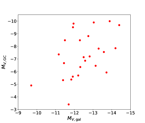
Figure 2: Relation between the absolute $V$ magnitude of the brightest GC and $M_{\scriptscriptstyle V,\rm gal}$ in the extended sample.

2 Sample of GCs in dwarf galaxies

We gather a sample of $38$ spectroscopically confirmed GCs plus $17$ candidates, around $26$ galaxies classified as dSph galaxies or transition-type galaxies (with properties intermediate between dIrr and dSph galaxies), using available data from the literature. Some relevant properties of the selected galaxies, such as their $V$ band absolute magnitudes $M_{\scriptscriptstyle V,\rm gal}$, and their effective radii $R_{e}$ (i.e. the projected half-light radii), are given in Table 1. We see that $M_{\scriptscriptstyle V,\rm gal}$ ranges between $-7.1$ and $-14.4$. We do not have the formal errors on $M_{\scriptscriptstyle V,\rm gal}$ for all galaxies, but they are known with an accuracy less than $0.3$ mag for Local Group dwarfs, and up to $0.5$ mag for low-surface brightness dSph galaxies outside the Local Group. We also provide the so-called tidal index $\Theta$, taken from Karachentsev et al. (2004), which is a measure of the level of isolation of the galaxies (see Section 7). Note that the Sagittarius dwarf galaxy has not been included because it is currently undergoing tidal disruption.

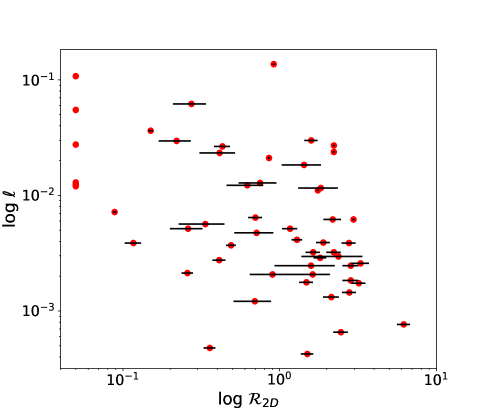
Figure 3: Relation between $\ell$ and $\mathcal{R}_{2\scriptscriptstyle\rm D}$ for GCs in the extended sample. For plotting purposes, in order to make the graph in logarithmic scale, we assigned a value of $\mathcal{R}_{2\scriptscriptstyle\rm D}=0.05$ to the central GCs. Typical fractional errors on $\ell$ are $\sim 30\%$.

Table 2 compiles the $V$ band magnitude, $M_{\scriptscriptstyle V,{\rm GC}}$, of each GC in our sample, as well as their projected distances from the host centre (denoted by $R_{\rm proj}$) and their estimated ages. In general, the typical uncertainty on $M_{\scriptscriptstyle V,{\rm GC}}$ is less than $0.1$ mag. As already said, we have $17$ GC candidates for which spectroscopic observations are required to rule out contamination by stellar interlopers projected onto the dSph galaxy, or by background galaxies (e.g., Da Costa et al., 2009). Still, there is little question that some of them (e.g., the one in KKs 55 or those in ESO 384-016) are real GCs (Georgiev et al., 2010; Forbes et al., 2018). For shortness, we will refer to the total sample of confirmed GCs plus candidates as the “extended” sample.

Hereafter, we will refer to central or NSCs as those sit at the centre of the host galaxy, i.e. $R_{\rm proj}=0$. In the sample of GCs under consideration, we have $6$ central GCs. And XXV Gep I is also considered as a central GC, although it is still unclear whether it is a central GC or the nucleus of And XXV (Cusano et al., 2016).

Table 2: Fundamental parameters of GCs in the extended sample

Name/ID	$M_{V}$	$R_{\rm proj}$	Age
		$(\arcsec)$	(Gyr)
(1)	(2)	(3)	(4)
Fornax GC 1⋆	$-5.34$	2400	$12.1\pm 0.8$
Fornax GC 2⋆	$-7.07$	1580	$12.2\pm 1.0$
Fornax GC 3⋆	$-7.82$	648	$12.3\pm 1.4$
Fornax GC 4⋆	$-6.90$	360	$10.2\pm 1.2$
Fornax GC 5⋆	$-7.07$	2160	$11.5\pm 1.5$
Eridanus II GC⋆	$-3.0$	13.9	$12.5\pm 1.5$
And I GC	$-3.4$	57	–
And XXV Gep I ⋆	$-4.9$	$\leq 11$	–
DDO 216-A1⋆	$-7.14$	6	$12.3\pm 0.8$
Sextans A-GC1⋆	$-7.85$	261	$8.6\pm 2.7$
KKs 3 GC⋆	$-8.48$	8.5	12.6
KKs 55-01	$-7.36$	77	–
KKs 58-NSC⋆	$-9.51$	0.0	$6.9\pm 1.0$
Sc 22 (Scl-dE1) GC1⋆	$-6.67$	20	–
IKN-01⋆	$-6.66$	98	14.77
IKN-02⋆	$-7.16$	76	–
IKN-03⋆	$-6.77$	38.5	13.21
IKN-04⋆	$-7.42$	20	14.19
IKN-05⋆	$-8.48$	12.3	13.80
BK6N 2-524	$-5.40$	43	–
BK6N 4-789	$-5.60$	65	–
KK 27 4-721	$-6.36$	31	–
KK 77 4-939	$-5.01$	71	–
KK 77 4-1162	$-5.37$	95	–
KK 77 4-1165	$-5.69$	95	–
KK 197-01⋆	$-5.75$	24.5	–
KK 197-02⋆	$-9.89$	0	$6.5\pm 1$
KK 197-03⋆	$-7.32$	8	$7\pm 1$
KK 211 3-917⋆	$-6.86$	29	$6\pm 2$
KK 211 3-149⋆	$-7.82$	0	$6\pm 2$
KK 221 2-608⋆	$-8.04$	70	–
KK 221 2-883⋆	$-7.07$	55	–
KK 221 2-966⋆	$-9.80$	28	$10\pm 2$
KK 221 2-1090⋆	$-7.77$	26	–
KK 221 24n⋆	$\sim-7.9$	70	$9\pm 2$
KK 221 27n⋆	$\sim-6.4$	94	–
DDO 78 1-167	$-7.23$	81	–
DDO 78 3-1082⋆	$-8.81$	14.5	$10.5\pm 1.5$
KDG 61 3-1325⋆	$-7.55$	2.86	$16\pm 2$
KDG 63 3-1168⋆	$-7.2$	12	$6\pm 2$
F8D1 GC	$-6.46$	14	–
ESO 269-66-01	$-8.08$	26.5	–
ESO 269-66-03⋆	$-9.99$	0	$12.6$
ESO 269-66-04	$-7.18$	63	–
ESO 269-66-05	$-7.18$	34	–
ESO 294-010 3-1104	$-5.32$	11	–
ESO 384-016-01	$-5.93$	129	–
ESO 384-016-02	$-5.29$	30.5	–
ESO 540-030 GC	$-5.37$	97	–
KK 84 2-785⋆	$-7.30$	52.5	–
KK 84 3-705⋆	$-8.38$	35.5	$9\pm 1$
KK 84 3-830⋆	$-9.68$	0	$10\pm 4$
KK 84 3-917⋆	$-7.52$	27.5	–
KK 84 4-666⋆	$-8.37$	52.2	$8\pm 3$
KK 84 12n⋆	$\sim-7.5$	60.5	–

Notes: Columns contain the following data: (1) name or ID, (2) absolute $V$ magnitude, (3) projected distance to the centre of the host galaxy in arcsec, (4) age. Asterisks after the name indicate those GCs that are spectroscopically confirmed. This data was collected from the references given in Table 1.

We define the specific luminosity of a certain GC as the ratio between its luminosity $L_{\scriptscriptstyle V,\rm GC}$ and the luminosity of the host galaxy $L_{\scriptscriptstyle V,\rm gal}$, that is $\ell\equiv L_{\scriptscriptstyle V,\rm GC}/L_{\scriptscriptstyle V,\rm gal}$. Figure 1 shows the distribution of the specific luminosity, and the distribution of ${\mathcal{R}}_{2\scriptscriptstyle\rm D}\equiv R_{\rm proj}/R_{e}$ in both the extended sample and for only confirmed GCs. The distributions of $\ell$ and ${\mathcal{R}}_{2\scriptscriptstyle\rm D}$ of the GCs in the extended sample are slightly different to those derived using the sample of confirmed GCs because all the central GCs have been confirmed spectroscopically. Aside from that, the distributions are very similar.

Throughout this paper, we only include the uncertainties associated with the determination of the effective radius $R_{e}$ of the galaxies. Uncertainties in the distance to the galaxies and those associated with photometry measurements (e.g., in $M_{\scriptscriptstyle V,\rm gal}$ and $M_{\scriptscriptstyle V,\rm GC}$) are not taken into account.

3 Searching for correlations

Correlations between different physical quantities are very useful to detect possible observational bias and to constrain suitable models. To evaluate possible correlations, we perform Spearman’s rank correlation tests. We consider that a correlation is strong when the Spearman’s coefficient $\rho_{s}$ is $\geq 0.6$, moderate when $0.4\leq\rho_{s}<0.6$, and weak when $\rho_{s}<0.4$. In addition to $\rho_{s}$, it is customary to give the $p$-value. A given correlation is considered significant if the probability ($p$-value) of getting a specific correlation coefficient by chance is lower than $5\%$ (i.e., $p<0.05$). However, when the sample is small, the information in the $p$-values is not complete. In such cases, it is more informative to estimate the $z$-score or the confidence level of the Spearman coefficient (Curran, 2015). Along this paper, we provide the $z$-scores but also the $p$-values for those readers that are more familiar with this indicator.

We first examine any possible correlation between the magnitude of the host galaxy $M_{\scriptscriptstyle V,{\rm gal}}$ and the magnitude $M_{\scriptscriptstyle V,{\rm GC}}$ of its most luminous GC (see Fig. 2). For GCs in the extended sample, the Spearman’s rank correlation coefficient is $\rho_{s}=0.52$ at a significance of $(3.0\pm 1.1)\sigma$ ($p$-value$<0.007$). This implies that there is a positive, albeit moderate, correlation between $M_{\scriptscriptstyle V,{\rm gal}}$ and the magnitude of the most luminous GCs. Assuming a constant stellar mass-to-light ratio for the galaxies and another constant value for the GCs, this relation is equivalent to the relation between the maximum GC mass and the host galaxy stellar mass. Leaman et al. (2020) have looked at this relation for a sample of Local Group galaxies with stellar masses up to $10^{11}M_{\odot}$. In the range of low stellar-mass galaxies (masses below $10^{8}M_{\odot}$), we find a similar scaling relation.

We have also performed the Spearman analysis for the correlation between $L_{\scriptscriptstyle V,{\rm gal}}$ and the total luminosity of the GC population in each galaxy, and found $\rho_{s}=0.50$ with a significance $z$-score of $(2.8\pm 1.2)\sigma$, using the extended sample. The $p$-value is $<0.01$. The correlation is moderate because of the short range in galaxy luminosities. A more clear positive trend between galaxy stellar mass and GC system mass is found when a wider range in galaxy luminosities is considered (e.g., Forbes et al., 2018; Leaman et al., 2020).

We have also searched for a correlation between the luminosity of the GCs and its distance to the host centre. As already said in the Introduction, there is some indications of mass segregation of GCs in dwarf galaxies. Mass segregation of GCs may be primordial if the most massive GCs were formed in the central regions, where converging flows of gas lead to reach high pressure. Dynamical friction of GCs against dark matter and field stars may also induce mass segregation since the dynamical friction time scales as the inverse of the GC mass.

The correlation between $L_{\scriptscriptstyle V,\rm GC}$ and the dimensionless projected radius $\mathcal{R}_{2\scriptscriptstyle\rm D}$ is $-0.28\pm 0.15$ for the GCs in the extended sample. If central GCs are excluded, the correlation is $-0.15\pm 0.15$. The correlation increases if the specific luminosity $\ell$ is considered instead of $L_{\scriptscriptstyle V,\rm GC}$. For the GCs in the extended sample, we find a relatively moderate anticorrelation with a coefficient of $\rho_{s}=-0.45\pm 0.12$, at a significance level of $(3.5\pm 1.1)\sigma$. The $p$-value is $6\times 10^{-4}$. A plot of $\ell$ versus $\mathcal{R}_{2\scriptscriptstyle\rm D}$ is shown in Figure 3. If we exclude the six NSCs, the correlation coefficient decreases to $-0.36\pm 0.14$. On the other hand, for the sample of confirmed GCs, we find $\rho_{s}=-0.46\pm 0.13$ between $\ell$ and $\mathcal{R}_{2\scriptscriptstyle\rm D}$, at a significance level of $(3\pm 1)\sigma$.

Since $R_{e}$ in our sample of galaxies only varies by a factor of $\sim 5$, being ESO 294-010 the galaxy with the lower $R_{e}$ ($233$ pc) and F8D1 with the largest $R_{e}$ ($1230$ pc), we have examined the correlation between $\ell$ and $R_{\rm proj}$ in parsecs. The difference between using $R_{\rm proj}$ or ${\mathcal{R}}_{2\scriptscriptstyle\rm D}$ is that the first one does not require knowledge of $R_{e}$, although is more sensitive to uncertainties in the adopted distances to the galaxies (which are not included here). We find that the strength of the correlation between $\ell$ and $R_{\rm proj}$ in the extended sample is $\rho_{s}=-0.45\pm 0.11$, with a $z$-score of $(3.5\pm 1.0)\sigma$. Remarkably, this correlation has the same strength as the $\ell$-${\mathcal{R}}_{2\scriptscriptstyle\rm D}$ correlation.

An inspection of the GCs in our sample indicates that the GC named KK 221-24n is very close to a bright foreground star (see the image in Fig. 2 of Puzia & Sharina 2008), making it difficult to obtain reliable photometry. If this GC is excluded of our extended sample, the strength of the anticorrelation between $\ell$ and $\mathcal{R}_{2\scriptscriptstyle D}$ increases to $\rho_{s}=-0.5$ at a significance of $(3.7\pm 1.1)\sigma$.

4 Monte Carlo model

GCs gradually sink towards the host centre due to the dynamical friction against the dark matter particles. In the central regions, the strength of dynamical friction depends on the underlying dark matter profile. For instance, in cored dark matter haloes, the rate of their inspiralling slows down when GCs reach the core radius (Meadows et al., 2020), or may potentially even stall (Goerdt et al., 2006; Inoue, 2009; Cole et al., 2012; Petts, Read & Gualandris, 2016; Leung et al., 2020). Therefore, the survival of GCs against orbital decay, their current positions, and the potential coalescence of multiple GCs to form NSCs depend on the dark matter profile. Indeed, some authors have put constraints on the dark matter density profile and on the initial galactocentric distance of the GCs in Fornax (e.g., Angus & Diaferio, 2009; Arca-Sedda & Capuzzo-Dolcetta, 2016; Meadows et al., 2020; Shao et al., 2021), DDO 216 [Pegasus dIrr galaxy] (Cole et al., 2017; Leaman et al., 2020) and Eridanus II (e.g., Amorisco, 2017; Contenta et al., 2018).

As said in the Introduction, there is no consensus about whether the timing problem of the orbital decay of Fornax GCs implies that its dark matter halo has a constant-density core. According to Meadows et al. (2020), the Fornax core radius required to solve the timing problem should be implausibly large. They suggest that the simplest explanation is that Fornax GCs were formed at radii of $\sim 2$ kpc (outside Fornax effective radius), and are now on their way to sinking to the centre (see also Angus & Diaferio, 2009; Shao et al., 2021). Did all massive GCs in dSph galaxies form in their outskirts?

In order to investigate further whether cuspy dark haloes are consistent with the current radial distribution of the observed GCs, we will assume that the dark matter haloes around dwarf galaxies are spherical, following an NFW profile, as predicted in cosmological $N$-body simulations:

$$\rho_{\rm dm}(r)=\frac{\rho_{0}r_{s}}{r\left(1+r/r_{s}\right)^{2}},$$ (1)

where $\rho_{0}$ and $r_{s}$ are scale parameters that vary from galaxy to galaxy. Nevertheless, we refer the reader to Section 7 for a discussion about the GC in-spiralling in cored dark matter haloes.

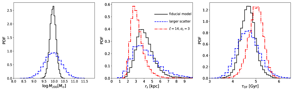
Figure 4: Probability distribution functions (PDFs) of $M_{200}$ (left panel), $r_{s}$ (middle panel) and $\tau_{\rm\scriptscriptstyle DF}$ (right panel) for a galaxy with $M_{V}=-13.3$, which corresponds to the Fornax $V$ band magnitude. Shown are histograms for our fiducial model (black solid lines), for a model where the scatter in the $M_{\star}$-$M_{200}$ relation is three times the nominal scatter in Read et al. (2017) (blue dashed histograms), and for a model where the distribution of $c$ is normal around a mean value $\bar{c}=14$ and standard deviation $\sigma_{c}=3$ (red dash-dotted histograms). $\tau_{\scriptscriptstyle\rm DF}$ is evaluated for a GC with $M_{\rm\scriptscriptstyle GC}=2\times 10^{5}M_{\odot}$ at an initial 3D distance of $1$ kpc.

Arca-Sedda et al. (2015) provide a useful interpolation formula for the dynamical friction timescale of massive point particles orbiting in spherical cuspy (or cored) density profiles with isotropic velocity distribution functions. The formula was calibrated against $N$-body models (Arca-Sedda et al., 2014). In their fitting process, the minimum impact parameter in the Coulomb logarithm varies along the orbit to properly account for the magnitude of the drag in the central parts where the density diverges and the local approximation overestimates it. In the particular case of an NFW profile, a GC with mass $M_{\scriptscriptstyle\rm GC}$ in an eccentric orbit with an initial apocentre $r_{\rm\scriptscriptstyle apo,i}$ reaches the centre after a time

$$\tau_{\scriptscriptstyle\rm DF}[{\rm Myr}]=0.3g(\tilde{e})\left(\frac{r_{s}}{1\,{\rm kpc}}\right)^{3/2}\left(\frac{M_{\rm gal}}{10^{11}M_{\odot}}\right)^{-1/2}\left(\frac{M_{\scriptscriptstyle\rm GC}}{M_{\rm gal}}\right)^{-0.67}\left(\frac{r_{\rm\scriptscriptstyle apo,i}}{r_{s}}\right)^{1.76},$$ (2)

where $M_{\rm gal}$ is the mass of the host galaxy, $\tilde{e}\equiv 1-(r_{\rm\scriptscriptstyle per,i}/r_{\rm\scriptscriptstyle apo,i})$ and $g(\tilde{e})\simeq 5-4\tilde{e}$. Here $r_{\rm\scriptscriptstyle per,i}$ is the initial pericentre. We will take the virial mass $M_{200}$ as a proxy for the mass of the host galaxy. Note that this expresion for the sinking time does not take into account mass loss of the GCs.

Assuming that the eccentricity is preserved during orbital decay, the apocentre of the GC decays to a value

$$r_{\rm\scriptscriptstyle apo,f}=\left(1-\frac{\tau}{\tau_{\rm\scriptscriptstyle DF}}\right)^{0.57}r_{\rm\scriptscriptstyle apo,i}$$ (3)

after a time $\tau$ (e.g., Arca-Sedda & Capuzzo-Dolcetta, 2016). Therefore, if we know the mass, the initial orbital parameters and the time at which the GCs started their orbital decay, as well as the scale parameters of the host dark matter haloes, we can compute the present-day orbital parameters of the GCs. If two or more GCs reach the centre in a certain galaxy, then we assume that they merge together and sum their luminosities. Conversely, Equation (3) allows to derive the past orbital parameters of the GCs if we knew their current values plus also the mass and scale radius of the dark matter haloes.

The validity of Equation (3) breaks down close to the centre of the host galaxy, typically at the galactocentric distance where the galaxy enclosed mass within the GC orbit is comparable to the GC mass (e.g. Gualandris & Merrit, 2008; Goerdt et al., 2010; Arca-Sedda et al., 2014). Indeed, this process may hinder the in-spiral of GCs in galaxies with shallow baryonic and total mass density profiles. In order to isolate the different effects and to properly intepret the results, we will omit this effect in Sections 5 and 6. The reader is referred to Section 7 for a discussion about the impact of this effect.

In order to estimate the parameters of the dark haloes of the sample galaxies, we first calculate the stellar mass of the galaxies, $M_{\star}$, from their luminosity assuming a uniform distribution of the stellar mass-to-light ratio $(M_{\star}/L)_{\scriptscriptstyle\rm gal}$ between $1$ and $2$ (Maraston, 2005; McConnachie, 2012). Once $M_{\star}$ is known, we use as default the stellar mass-halo mass relation for low-mass galaxies, as found in Read et al. (2017), including the reported confidence intervals, to assign $M_{200}$ to each galaxy. Read et al. (2017) fit the rotation curves of a ‘clean’ sample of isolated dwarf galaxies plus Carina dSph galaxy and Leo T, and found a monotonic relation between $M_{\star}$ and $M_{200}$ with little scatter. As a test of the $\Lambda$CDM model, they compare this relation with the $M_{\star}$-$M_{200}$ relation obtained from abundance matching technique, using the stellar mass function from Sloan Digital Sky Survey (SDSS), and found good agreement. We caution, however, that the $M_{\star}$–$M_{200}$ relation in dwarf galaxies is still an active field of research: galaxy formation models predict values of $M_{200}$ above those derived from abundance matching with field galaxies (e.g., Contenta et al., 2018; Forbes et al., 2018). In addition, many of the dSph galaxies in our sample are satellites that may have suffered tidal stripping. This could move dSph galaxies off of the $M_{\star}$-$M_{200}$ relation of isolated dwarf galaxies, probably leading to a value of $M_{200}$ below those derived from abundance matching (e.g., Errani et al., 2018). Given the uncertainties in the $M_{\star}$-$M_{200}$ relation, we will explore below how $\tau_{\scriptscriptstyle\rm DF}$ depends on the assumed scatter in this relation.

Besides $M_{200}$, we use the concentration parameter $c$ to characterize the NFW profile of dark matter haloes. We sample the concentration $c$ using the distribution function given in Shao et al. (2021) (their figure 2). These authors fit an NFW profile to field galaxies with stellar mass between $2\times 10^{7}M_{\odot}$ and $8\times 10^{7}M_{\odot}$ formed in the E-MOSAICS simulation. The distribution function of the concentration has a median value of $c=10.5$, a value consistent with previous high-resolution cosmological simulations.

For illustration, Figure 4 shows the distribution function of $M_{200}$ and $r_{s}$ for a galaxy with the luminosity of Fornax. For our fiducial model, the halo mass peaks at a value of $10^{10}M_{\odot}$, whereas $r_{s}$ peaks at $4$ kpc. This halo mass is larger than the value adopted by other authors (e.g., $2.7\times 10^{9}M_{\odot}$ in Meadows et al., 2020), but consistent with the mass estimate derived by Read et al. (2019), $(2.2\pm 0.7)\times 10^{10}M_{\odot}$, using abundance matching (see also Shao et al., 2021). On the other hand, our estimate of $r_{s}$ is larger than the value estimated in Meadows et al. (2020) ($2.1$ kpc), but smaller than the median value ($6$ kpc) found in E-MOSAICS by Shao et al. (2021). To illustrate the sensitivity of the inspiral rate on the uncertainties in the $M_{\star}$-$M_{200}$ relation, Figure 4 also shows $\tau_{\rm\scriptscriptstyle DF}$ of a GC with a mass of $2\times 10^{5}M_{\odot}$ (which is the median mass of Fornax GCs) at an initial radius of $1$ kpc using the amount of scatter described above, but also when the amount of scatter in $M_{200}$ for a given stellar mass $M_{\star}$ has been tripled. We see that it has little impact on the value of $\tau_{\rm\scriptscriptstyle DF}$. Finally, we also show the corresponding distributions if, instead of the distribution function of the concentration given in Shao et al. (2021), we sample the concentration using a normal distribution around $c=14$ with $\sigma_{c}=3$ (e.g., Dutton & Macciò, 2014). A larger concentration index implies a smaller $r_{s}$ and a slightly longer ($10$ percent) $\tau_{\rm\scriptscriptstyle DF}$.

It is likely that tidal forces and energetic outflows from bursty star formation can kinematically heat up the dark matter at the central parts, forming cores. Dwarf-dwarf mergers could also push the GCs towards more extended orbits. By ignoring these effects, we are overestimating the rate of orbital decay of GCs (see Section 7).

A trial of the GC system is performed by assigning either $38$ or $55$ GCs, depending if we use only the spectroscopically confirmed GCs or the extended sample, to their respective galaxies. The mass of each GC, $M_{\scriptscriptstyle\rm GC}$, is computed from its magnitude, whose values are given in Table 2, and the mass-to-light ratio $(M/L)_{\scriptscriptstyle\rm GC}$. The latter quantity, $(M/L)_{\scriptscriptstyle\rm GC}$, is randomly drawn from a uniform distribution between $1.5M_{\odot}/L_{\odot}$ and $2.5M_{\odot}/L_{\odot}$ (McLaughlin & van der Marel, 2005).

The time since GCs started orbital decay, $\tau_{\scriptscriptstyle\rm GC}$, corresponds to their age $\tau_{\rm age}$ for in-situ GCs, but it is less than their age for accreted GCs. There is no a simple way to distinguish between in-situ and accreted GCs. Although there are indications of late time mergers (e.g., Coleman et al. 2004), accretion of the GCs by dwarf-dwarf mergers are expected to occur mosty at redshifts $z\geq 2$ (corresponding to $\geq 9$ Gyr). As a result, accreted GCs tend to be old, whereas GCs younger than $7$ Gyr are expected to be in-situ GCs. Therefore, we will assume that the five GCs with estimated ages between $6$ and $7$ Gyr in Table 2 are in-situ GCs, and we take for $\tau_{\scriptscriptstyle\rm GC}$ the reported age values including their uncertainties. For the remainder GCs, $\tau_{\scriptscriptstyle\rm GC}$ is randomly drawn from a uniform distribution between $6$ and $12$ Gyr. In fact, all those GCs have $\tau_{\rm age}$ consistent with $12$ Gyr (within one standard deviation), except one. Note also that $55\%$ of the GCs in our sample has no age determination. Therefore, a range of $\tau_{\scriptscriptstyle\rm GC}$ between $6$ and $12$ Gyr seems reasonable. However, we also present results assuming that all GCs are in-situ and evolve for the full age.

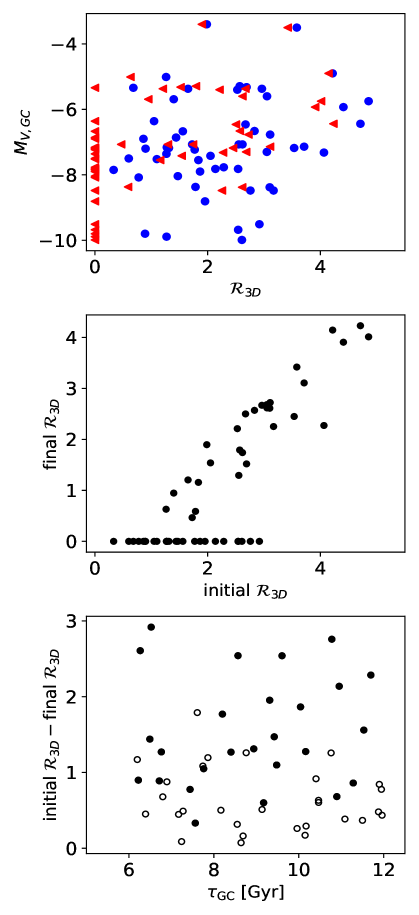
Figure 5: Evolution of the 3D distance from the host centre of GCs due to dynamical friction in a realization with $\lambda=2$. The upper inset shows the starting radii (blue points) and the final radii (red triangles) in the plane $\mathcal{R}_{3\scriptscriptstyle\rm D}$–$M_{\scriptscriptstyle V,\rm GC}$. The middle inset displays the final versus the starting values of $\mathcal{R}_{3\scriptscriptstyle\rm D}$ in the same realization. The lower panel shows the change in the orbital radius versus $\tau_{\scriptscriptstyle\rm GC}$. Solid dots mark those GCs that have sunk to the centre.

Note that we are not including mass loss of GCs in our models. If GCs were more massive in the past, the dynamical friction timescale would become shorter (e.g., Amorisco, 2017). Therefore, our assumption of constant $M_{\rm\scriptscriptstyle GC}$ is underestimating dynamical friction. The problem of the survival of low-mass GCs that lie in the central regions (at least in projection) against tidal forces, such as Eridanus II GC or DDO 216-A1, is an interesting issue that may provide additional constraints to the distribution of dark matter (e.g., Amorisco, 2017; Contenta et al., 2018; Leaman et al., 2020).

In the next section, we will assume a simple distribution of the starting GC distances and compare the expected present-day radial distribution of GCs with the observed one. In Section 6, we take the current projected distances of the GCs and use Equation (3) to infer their past and future positions.

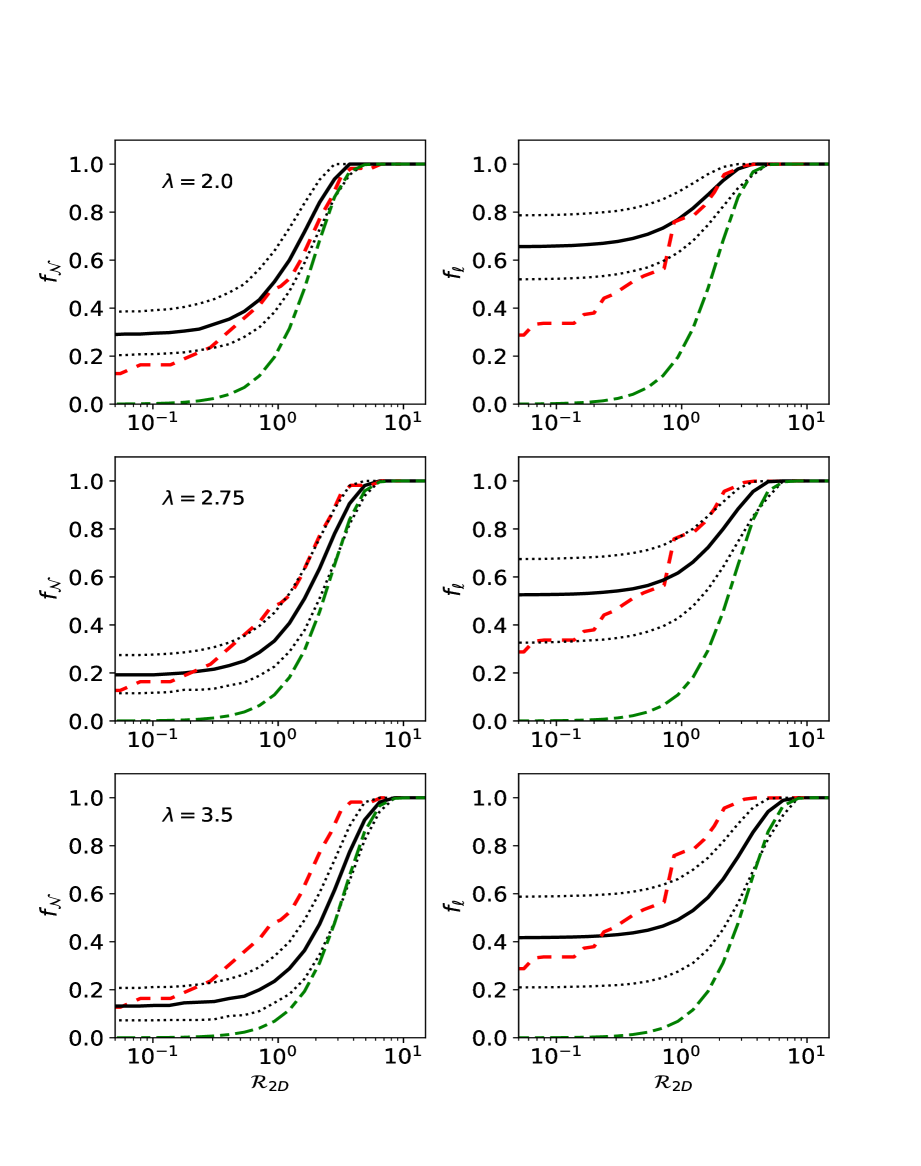
Figure 6: Fraction of GCs (left panels) and fraction of specific luminosity (right panels) enclosed within a circle of radius $\mathcal{R}_{2\scriptscriptstyle\rm D}$ from the centre of the galaxies, for three values of $\lambda$. The red dashed lines show the observed distributions in the extended sample. The black curves are the predicted distributions in our Monte Carlo model at the present day (solid lines indicate the median value and the dotted lines encompass the $95.4$ percent of the Monte Carlo simulations). The green dashed lines show the initial distributions.

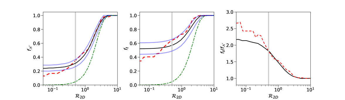
Figure 7: Radial dependence of $f_{\scriptscriptstyle\mathcal{N}}$ (left panel), $f_{\ell}$ (midlle panel) and $f_{\ell}/f_{\scriptscriptstyle\mathcal{N}}$ (right panel), excluding KK 221 2-966. The black, red and green lines have the same meaning as in Figure 6. The lower blue lines and the upper blue lines indicate the $16$th and $84$th percentiles, respectively. In these models, we assume $\lambda=2.3$. The vertical lines mark the radial distance $\mathcal{R}_{2\scriptscriptstyle\rm D}=0.5$.

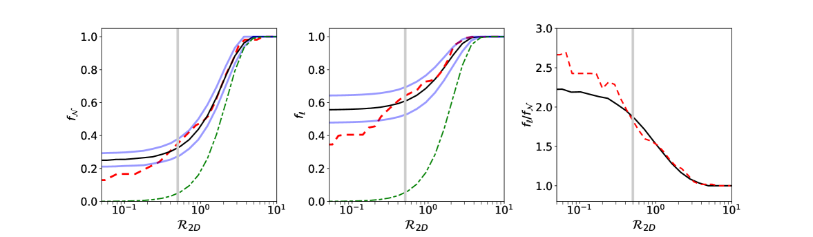
Figure 8: Same as Figure 7 but using $\lambda=2.1$ for GCs with $\ell>0.005$ and $\lambda=2.4$ for GCs having $\ell\leq 0.005$ (excluding KK 221 2-966).

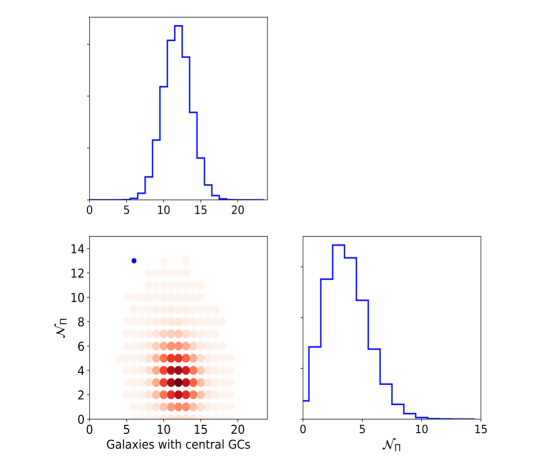
Figure 9: Corner plot showing the correlation and distributions of the number of galaxies with a central GC and $\mathcal{N}_{\Pi}$ (the number of GCs inside $\mathcal{R}_{2\scriptscriptstyle\rm D}=0.5$, but excluding central ones), at the present epoch, in a model with $\lambda=2.3$. The blue dot indicates the data point in that plane.

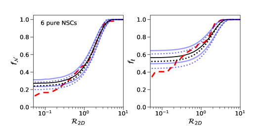
Figure 10: Radial dependence of $f_{\scriptscriptstyle\mathcal{N}}$ and $f_{\ell}$ in a model where the six NSCs are assumed to have formed in situ at the galaxy centre, i.e. they are pure NSCs (solid lines). The starting radial distances of the other GCs are given by Equation (4) with scale $\lambda=2.3$. To facilitate comparison, the corresponding curves for the fiducial model (without assuming pure NSCs) are also shown (dotted lines). Line colours are the same as Figures 7 and 8.

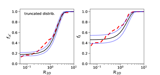
Figure 11: $f_{\scriptscriptstyle\mathcal{N}}$ and $f_{\ell}$ versus $\mathcal{R}_{2\scriptscriptstyle D}$ in a model where the distribution of starting radial distances is given by Equation (4) with scale $\lambda=2.3$, but truncated at an inner radius $\mathcal{R}_{2\scriptscriptstyle\rm D}=1.5$ and at an outer truncation radius $\mathcal{R}_{2\scriptscriptstyle\rm D}=4.6$.

5 What to expect if the initial radial distribution is Gaussian. A heuristic approach

5.1 Fiducial model

It is convenient to define $\mathcal{R}_{3\scriptscriptstyle\rm D}$ as the $3$D distance to the host centre in units of the galaxy effective radius. As the simplest starting assumption, we consider in this section that the orbits of the surviving GCs are almost circular, i.e. $\tilde{e}=0$, and the probability distribution function (PDF) of ${\mathcal{R}}_{3\scriptscriptstyle\rm D}$, that is the probability that a GC has a starting distance ${\mathcal{R}}_{3\scriptscriptstyle\rm D}$, is

$${\mathcal{N}}_{\rm GC}^{(i)}({\mathcal{R}}_{3\scriptscriptstyle\rm D})=4\pi^{-1/2}\lambda^{-3}\mathcal{R}_{3\scriptscriptstyle\rm D}^{2}\exp\left(-\left[\frac{\mathcal{R}_{3\scriptscriptstyle\rm D}}{\lambda}\right]^{2}\right),$$ (4)

where $\lambda$ is a dimensionless free parameter. The superscript $(i)$ indicates that the distribution is the initial one. The above distribution indicates that the volume probability density for a GC to start at $\mathcal{R}_{3\scriptscriptstyle\rm D}$ is Gaussian. The corresponding PDF of $\mathcal{R}_{2\scriptscriptstyle\rm D}$ is

$${\mathcal{N}}_{\rm GC}^{(i)}({\mathcal{R}}_{2\scriptscriptstyle\rm D})=2\lambda^{-2}\mathcal{R}_{2\scriptscriptstyle\rm D}\exp\left(-\left[\frac{\mathcal{R}_{2\scriptscriptstyle\rm D}}{\lambda}\right]^{2}\right).$$ (5)

Thus, the effective radius of the GC system as a whole is $\sqrt{\ln 2}\lambda R_{e}$. In this simple model, the starting position of the GCs is correlated neither with its mass, i.e. there is no mass segregation initially, nor with its age.

The way to set the initial radius of GCs in the Monte Carlo model is as follows. In each trial, we draw the initial $\mathcal{R}_{3\scriptscriptstyle\rm D}$ from the PDF given in Equation (4). We next convert them into physical units by sampling the effective radius of each galaxy $R_{e}$ from a normal distribution around the observed mean value and the $1\sigma$ uncertainty, which are given in Table 1. Following the method described in the previous section, we can derive the radial distributions of $\mathcal{R}_{3\scriptscriptstyle\rm D}$, $\mathcal{R}_{2\scriptscriptstyle\rm D}$, and $\ell$ at the present day.

Figure 5 shows the starting and the final distances $\mathcal{R}_{3\scriptscriptstyle\rm D}$ of the GCs, in a realization of $55$ GCs with $\lambda=2$. It is clear that GCs far away from the centre of the host galaxy undergo comparatively less orbital decay because the density of dark matter is comparatively small. Inner GCs are expected to experience more friction. In that particular realization, we can see that most of the GCs that starts within $\sim 1.5R_{e}$ sink to the centre of their host galaxies, regardless their magnitude $M_{\scriptscriptstyle V,\rm GC}$. For those GCs starting at distances larger than $2R_{e}$, only the most luminous and hence the most massive GCs suffer an appreciable change in their orbital radii. In a large fraction of the trials, the five most luminous GCs sink to the centre. From the lower panel, we see that the values of $\tau_{\rm\scriptscriptstyle GC}$ of those GCs that reach the centre span across the whole $\tau_{\rm\scriptscriptstyle GC}$ range.

Figure 6 shows the starting and the present-day cumulative distributions of projected distances, denoted by $f_{\scriptscriptstyle\mathcal{N}}(\mathcal{R}_{2\scriptscriptstyle\rm D})$, for $\lambda=2.0,2.75$, and $3.5$. We also show $f_{\ell}(\mathcal{R}_{2\scriptscriptstyle\rm D})$, which is defined as the fraction of specific luminosity contained inside a projected radius $\mathcal{R}_{2\scriptscriptstyle\rm D}$. At each radius ${\mathcal{R}}_{2\scriptscriptstyle\rm D}$, we provide the median value and $2.3$th and $97.7$th percentiles of the distributions after $1.2\times 10^{5}$ realizations. We also plot $f_{\scriptscriptstyle\mathcal{N}}$ and$f_{\scriptscriptstyle\ell}$ as derived from the observational data.

For $\lambda=2$, approximately $30\%$ of the GCs sink to the host galaxy centre at the present day (top left panel). These central GCs contain more than $60\%$ of the total specific luminosity (top right panel). Due to the inspiraling of GCs, the effective radius of the GC system (i.e. the radius at which $f_{\scriptscriptstyle\mathcal{N}}=0.5$), changes from $1.66R_{e}$ initially to $0.92R_{e}$ at the present day. As expected, the number of GCs that sink to the host centre decreases with $\lambda$. In order to account for the observed fraction of GCs at $\mathcal{R}_{2\scriptscriptstyle\rm D}=0.1$, a value of $\lambda\simeq 3.5$ is required. However, this model underpredicts the number of GCs over a large radial range. For $\lambda=2.75$, $f_{\ell}$ at $\mathcal{R}_{2\scriptscriptstyle\rm D}=0.1$ is larger than the observed value in $97.7$ percent of the trials (middle right panel in Fig. 6). At $1<\mathcal{R}_{2\scriptscriptstyle\rm D}<4$, however, more than $97.7$ percent of the trials give smaller values for $f_{\scriptscriptstyle\mathcal{N}}$ and $f_{\ell}$ than the observed ones.

We noticed that the GC KK 221 2-966 sinks to the centre of the host galaxy in a significant fraction of the trials if $\lambda\leq 3.0$. However, the current 2D distance of this GC is $0.85R_{e}$. Indeed, the jump in $f_{\ell}$ at $\mathcal{R}_{2\scriptscriptstyle\rm D}=0.85$ visible in the observed distribution of the extended sample (red dashed curves in the right panels of Figure 6) is due to the contribution to $\ell$ by KK 221 2-966. In fact, the form of $f_{\ell}$ versus $\mathcal{R}_{2\scriptscriptstyle\rm D}$ is dominated by the radial distance of the most luminous GCs. This produces that $f_{\ell}$ is generally less smooth than $f_{\scriptscriptstyle\mathcal{N}}$. Therefore, we decided to explore how the radial distributions change when this GC is excluded from the analysis and it is studied separately (see Section 6.1).

Figure 7 shows the radial distributions derived from the observational data, together with the expected distributions for a model with $\lambda=2.3$, once KK 221 2-966 is excluded. To facilitate the discussion, let us first focus on the region $\mathcal{R}_{2\scriptscriptstyle\rm D}\gtrsim 0.5$. We see that the predicted curve of $f_{\scriptscriptstyle\mathcal{N}}$ follows quite well the distribution as derived from the data. Between $\mathcal{R}_{2\scriptscriptstyle\rm D}=0.5$ and $\mathcal{R}_{2\scriptscriptstyle\rm D}=1$, the observed values of $f_{\scriptscriptstyle\mathcal{N}}$ and $f_{\ell}$ are larger than the predicted median values, but they lie within the $68$th percentile. The enhancements in the observed values of $f_{\scriptscriptstyle\mathcal{N}}$ and $f_{\ell}$ are correlated, so that the ratio $f_{\ell}/f_{\scriptscriptstyle\mathcal{N}}$ follows the ratio expected in that model. In the case under consideration, the curve $f_{\ell}/f_{\scriptscriptstyle\mathcal{N}}$ as derived from the data is sligthly above the predicted curve. In addition, the correlation coefficient between $\ell$ and $\mathcal{R}_{2\scriptscriptstyle\rm D}$, denoted by $\hat{\rho}_{s}$, is $-0.45\pm 0.12$ for the observed distribution, whereas it is $-0.31\pm 0.11$ in our Monte Carlo model with $\lambda=2.3$ . Although these values of $\hat{\rho}_{s}$ are consistent at $1\sigma$ level, $\hat{\rho}_{s}$ can be enhanced by introducing some degree of primordial mass segregation. For instance, if we split the population of GCs into two halves; those having $\ell>0.005$ and those with $\ell<0.005$, and assign a scalelength parameter of $\lambda=2.1$ for the first group and $\lambda=2.4$ for second group, the initial value of $\hat{\rho}_{s}$ is $-0.12\pm 0.13$, and its final value is $-0.39\pm 0.11$, which is closer to the real value. The resulting distributions in this two-Gaussian model are shown in Figure 8. We find that the global properties of the observed radial distribution of GCs at distances $\mathcal{R}_{2\scriptscriptstyle\rm D}\gtrsim 0.5$, once the massive GC KK 221 2-966 is excluded, can be reasonably accounted for in a two-Gaussian model.

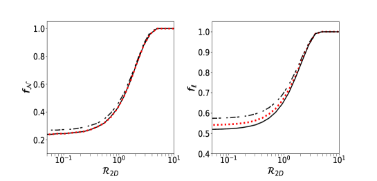
Figure 12: Distributions $f_{\scriptscriptstyle\mathcal{N}}$ and $f_{\ell}$, adopting different recipes for $\tau_{\scriptscriptstyle\rm GC}$. Black solid lines correspond to our fiducial model described in Section 4. Black dash-dotted lines are the results when adopting $\tau_{\rm\scriptscriptstyle GC}=\tau_{\scriptscriptstyle\rm age}$, and a uniform distribution over the interval $[6,13.5]$ Gyr for those GCs that have no estimates of their ages. Finally, red dotted curves correspond to the results assuming $\tau_{\rm\scriptscriptstyle GC}=\tau_{\scriptscriptstyle\rm age}$ for those having age estimates, and $\tau_{\rm\scriptscriptstyle GC}=7$ Gyr for those that do not have age estimates. In all these models, we assume $\lambda=2.3$.

Consider now the radial GC distribution at $\mathcal{R}_{2\scriptscriptstyle\rm D}\lesssim 0.5$. The predicted functions $f_{\scriptscriptstyle\mathcal{N}}$ and $f_{\ell}$ at $\mathcal{R}_{2\scriptscriptstyle\rm D}<0.5$ for $\lambda=2.3$ are shallower than the observed distributions (Figure 7). The predicted values of $f_{\scriptscriptstyle\mathcal{N}}(0)$ and $f_{\ell}(0)$ for the model with $\lambda=2.3$ are higher than the observed values. Note that $f_{\scriptscriptstyle\mathcal{N}}(0)$ is the fraction of central GCs. In the data sample, six galaxies have a central GC. However, in only $0.2\%$ of the trials in a model with $\lambda=2.3$, six galaxies (or less) have a central GC (see Figure 9). In fact, the expected number of galaxies with a central GC is $12\pm 2$ (excluding KK 221 2-966 in the analysis).

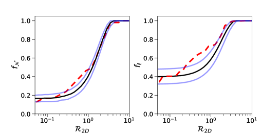
Figure 13: Radial profiles of $f_{\scriptscriptstyle\mathcal{N}}$ and $f_{\ell}$ in a model where the value of $\tau_{\rm\scriptscriptstyle DF}$, given in Equation (2), is increased by a factor of $2$. The distribution of starting distances is given by Equation (4) with $\lambda=2.0$. Line colours and style codes are the same as those used in Figures 7, 8, 10 and 11.

We also observe a discrepancy between the observed and the predicted slope of $f_{\scriptscriptstyle\mathcal{N}}$ at $\mathcal{R}_{2\scriptscriptstyle\rm D}\lesssim 0.5$, which indicates a discrepancy in the number density of GCs. To make a quantitative comparison, it is useful to define $\mathcal{N}_{\Pi}$ as the number of GCs with projected radii $0<\mathcal{R}_{2\scriptscriptstyle\rm D}<0.5$ (excluding the nuclei). More formally, $\mathcal{N}_{\Pi}=[f_{\scriptscriptstyle\mathcal{N}}(0.5)-f_{\scriptscriptstyle\mathcal{N}}(0)]N_{\scriptscriptstyle\rm GC}$, where $N_{\scriptscriptstyle\rm GC}$ is the total number of GCs. In our extended sample of GCs, the value is $\mathcal{N}_{\Pi}=13$. However, the model with $\lambda=2.3$ predicts $\mathcal{N}_{\Pi}=4\begin{subarray}{c}+1\\ -2\end{subarray}$ because there GCs spend little time given that dynamical friction is strong. Figure 9 shows the probability distribution of $\mathcal{N}_{\Pi}$ and the correlation between $\mathcal{N}_{\Pi}$ and the number of galaxies hosting a NSC. In this model, the probability that $\mathcal{N}_{\Pi}\geq 13$ is $\sim 8\times 10^{-5}$. This discrepancy between predictions and observed values is also obtained when realizations of the $38$ confirmed GCs are carried out.

In the two-Gaussian model, which includes some degree of primordial mass segregation, the discrepancy between the predicted distributions and the distributions derived from observations at $\mathcal{R}_{\scriptscriptstyle 2D}<0.5$ increases, especially for $f_{\ell}$. The reason is that in this model the most luminous GCs are initially more spatially concentrated, so that the GCs that arrive to radii $\mathcal{R}_{\scriptscriptstyle 2D}<0.5$ are, on average, more luminous than in a model without primordial mass segregation.

In order to find possible explanations for the offset in the value of $\mathcal{N}_{\Pi}$ from the model distribution, it is worth bearing in mind that, in our extended sample of GCs, $12$ galaxies contribute to $\mathcal{N}_{\Pi}$. Only IKN has two GCs at $0<\mathcal{R}_{\scriptscriptstyle 2D}<0.5$. Therefore, none of the galaxies predominantly contributes to the value of $\mathcal{N}_{\Pi}$. On the other hand, in this subsample of $12$ galaxies that contribute to $\mathcal{N}_{\Pi}$, one galaxy (KK 197) has also a NSC. Given that the fraction of galaxies hosting a GC is $6/55$ in our extended sample, about one galaxy is indeed expected to have a NSC in a sample of $12$ galaxies, as long as there is no correlation between hosting a GC at $0<\mathcal{R}_{\scriptscriptstyle 2D}<0.5$ and the possession of a NSC.

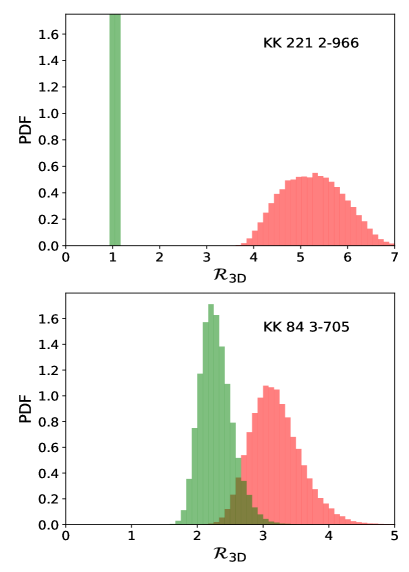
Figure 14: Distribution of the present (green histograms) and starting (red histograms) 3D distances for KK 221 2-966 (top panel) and KK 84 3-705 (bottom panel).

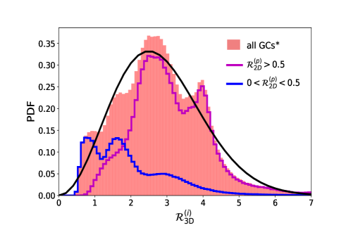
Figure 15: Histograms of the distribution of the starting orbital radii of GCs, $\mathcal{N}_{\scriptscriptstyle\rm GC}^{(i)}$, in the full sample excluding central GCs (orange), together with the contributions from GCs having $0<\mathcal{R}_{\scriptscriptstyle 2D}^{(p)}<0.5$ (blue histogram) and from GCs with $\mathcal{R}_{\scriptscriptstyle 2D}^{(p)}>0.5$ (magenta). The solid black line corresponds to the graph of the function given in Equation (4) with $\lambda=2.5$.

5.2 Variations of the fiducial model

As said in Section 2, six GCs in our sample reside at the centre of their host galaxies (And XXV Gep I, KKs 58-NSC, KK 197-02, KK 211 3-149, ESO 269-66-03 and KK 84 3-830). It is plausible that some of these central GCs did not inspiral towards the centre but they were formed in situ at the centre of the host galaxy. From Table 2, we see that four of these GCs are more luminous than magnitude $-9.5$ (see also Figure 3). In the in-situ formation scenario, an explanation for the NSCs being more luminous than non-central GCs could be that NSCs grow their stellar mass by sustained star formation due to the large amounts of gas available at the centre. We do not know what NSCs in our sample were formed at the centre and what NSCs spiralled into the centre. We have computed $f_{\scriptscriptstyle\mathcal{N}}$ and $f_{\ell}$ in the extreme situation where the six abovementioned NSCs are assumed to be formed in situ at the galaxy centres. For these GCs we set their initial orbital radius to zero and proceed following the Monte Carlo scheme described in Section 4. The initial orbital radii of non-central GCs are drawn from the distribution given in Equation (4). Figure 10 shows the predicted distributions for the fiducial value of $\lambda$. As expected, the predicted value of $f_{\scriptscriptstyle\mathcal{N}}(0)$ becomes larger (more discrepant with the observed values) if some of the central GCs are pure NSCs.

The large fraction of galaxies with a central GC predicted in a model with $\lambda=2.3$ can be alleviated by introducing inner and outer truncation radii to the starting spatial distribution of GCs given in Equation (4). For instance, Figure 11 shows the radial distributions for $\lambda=2.3$, but assuming that no GCs were born or started its orbital decay inside $1.5R_{e}$ and beyond $4.6R_{e}$. In that model, the probability of having six (or less) galaxies with a central GC is $5\%$. However, the predicted value of $\mathcal{N}_{\Pi}$ is still low as compared to the value derived from the observational data. Moreover, it is hard to explain the origin of the internal truncation on the basis that stellar cluster formation should have been more likely in the inner regions ($<1.5R_{e}$) of the galaxy, where a larger gas reservoir has been available to promote GC formation.

The difference $f_{\scriptscriptstyle\mathcal{N}}(0.5)-f_{\scriptscriptstyle\mathcal{N}}(0)$ is rather insensitive to the value of $\lambda$, as can be seen in Figure 6, implying that $\mathcal{N}_{\Pi}$ is also insensitive. It is worth to check if $\mathcal{N}_{\Pi}$ is sensitive to our recipe for $\tau_{\scriptscriptstyle\rm GC}$. In our fiducial model, we consider that some of the GCs with $\tau_{\rm age}>7$ Gyr could be potentially ‘ex-situ’ GCs. For them, we assumed a uniform distribution of $\tau_{\rm\scriptscriptstyle GC}$ between $6$ and $12$ Gyr. In order to quantify the impact of this assumption, Figure 12 shows $f_{\scriptscriptstyle\mathcal{N}}$ and $f_{\ell}$ when all the GCs are treated as in-situ GCs. More specifically, we take $\tau_{\rm\scriptscriptstyle GC}=\tau_{\rm age}$ for all the GCs having age estimates as given in Table 2. For those GCs with no age measurements, we explore two scenarios: (i) all of them have $\tau_{\rm\scriptscriptstyle GC}=7$ Gyr and (ii) $\tau_{\rm\scriptscriptstyle GC}$ follows a uniform probability distribution in the range $[6,13.5]$ Gyr. We see that the final distribution of GCs is slightly more centrally concentrated in the second case. However, the value of $\mathcal{N}_{\Pi}$ in these two variations is essentially the same as in the fiducial model.

To compute the evolution of the orbital radius of the GCs, we have used the Arca-Sedda et al. (2015) formula. To derive that formula, they carried out a careful modelling to include correctly the contribution to the drag from particles deep in the cuspy region of the galaxy. Still, we have explored the impact on the results if the dynamical friction timescale $\tau_{\rm\scriptscriptstyle DF}$ given in Equation (2) is doubled. Figure 13 shows the predicted radial distributions for such a case and assuming $\lambda=2$. We find that the number of galaxies with a central GC would be $8\begin{subarray}{c}+2\\ -1\end{subarray}$, which is close to the observed value. On the other hand, the predicted value of $\mathcal{N}_{\Pi}$ in this model is $4\begin{subarray}{c}+3\\ -1\end{subarray}$, with a $4.5\times 10^{-4}$ probability that $\mathcal{N}_{\Pi}\geq 13$. This reduction in the dynamical friction strength is not enough to reconcile models with the data. As expected, a reduction in dynamical friction implies a more compact initial distribution of the GCs, i.e., a smaller value of $\lambda$. This does not result in an enhancement of the correlation between $\ell$ and $\mathcal{R}_{2\scriptscriptstyle\rm D}$; we find a correlation coefficient $\hat{\rho}_{s}=-0.25\pm 0.12$ in this case.

In summary, we have adopted an NFW profile for the dark haloes of dSph galaxies and find that the radial distribution of the GCs at distances $\mathcal{R}_{2\scriptscriptstyle\rm D}>0.5$ can be fitted reasonably well by assuming a simple distribution for the starting GC distances. However, even adopting rather artificial starting positions for the GCs, such as truncated distributions, it is difficult to account for the relatively high number of GCs inside $\mathcal{R}_{2\scriptscriptstyle\rm D}=0.5$, that are caught in their journey inwards. This is seen as a timing problem. In Section 7 we discuss the impact of some omitted processes, such as the stalling of the dynamical friction when the enclosed mass is comparable to the GC mass. Before that, we present complementary views of the timing problem in the next section.

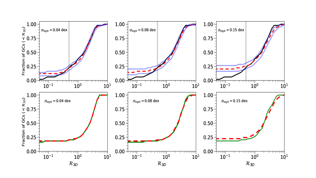
Figure 16: Cumulative distributions of 3D distances of the non-central GCs at the present epoch. In the top panels, the black lines represent the present-day distribution from the data, the red dashed lines indicate the median of the present-day distributions when the starting radii of the GCs are taken as $\mathcal{R}_{3{\scriptscriptstyle\rm D},j}^{(i)}+\delta\mathcal{R}_{j}^{(i)}$, i.e. they are shifted from their original values in each trial, with $\sigma_{\scriptscriptstyle{\rm log}\mathcal{R}}=0.04$ dex (left panels), $0.08$ dex (central panels) and $0.15$ dex (right panels). Blue lines indicate the $16$th and $84$th percentiles of the distributions. As a guide for the eye, the vertical lines mark the radial distance $\mathcal{R}_{3\scriptscriptstyle\rm D}=0.5$. In the bottom panels, we take a random set of $\mathcal{R}_{3{\scriptscriptstyle\rm D},j}^{(i)}$ using the PDF given in Equation (4) with $\lambda=2.3$, and compute the present-day cumulative distributions without adding “noise” (green curves) and adding “noise” to the starting GC distances (red dashed lines).

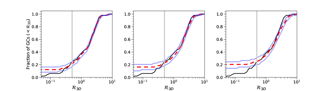
Figure 17: Same as top panels in Figure 16 but the values of $R_{e}$, $(M_{\star}/L)_{\rm\scriptscriptstyle gal},(M/L)_{\rm\scriptscriptstyle GC},M_{200},c$ and $\tau_{\rm\scriptscriptstyle GC}$ have been fixed to their median values, i.e. they are not treated as random variables.

6 Past and future orbital radii of the GCs: Alternative views of the timing problem

6.1 Starting GC distances

In the previous section we have assumed the distribution of the starting orbital radii of the GCs and computed the present-day distribution. Then we have compared the resultant radial configurations of the GCs with the observed ones. One benefit of that approach is that projection effects are included in a natural way, because the Monte Carlo models contain information about both $3$D and projected radii of the GCs.

An alternative approach consists of computing the starting orbital radii from the current projected distances of the GC. To do so, we have to estimate the present-day $3$D distance of each GC, $\mathcal{R}^{(p)}_{3{\scriptscriptstyle\rm D},j}$, where the superscript $p$ indicates ‘present’ and the index $j$ refers to the $j^{\rm th}$ GC. In principle, it is possible to do that using deprojection techniques. However, given the small number of GCs in our sample, we assume that $\mathcal{R}^{(p)}_{3{\scriptscriptstyle\rm D},j}=\sqrt{3/2}R_{2{\rm\scriptscriptstyle D},j}^{(p)}$ (Meadows et al., 2020; Shao et al., 2021). For those GCs that are not at the centre of the host galaxy (i.e. $\mathcal{R}^{(p)}_{3{\scriptscriptstyle\rm D},j}\neq 0$), we invert Equation (3) to find the starting distance $\mathcal{R}^{(i)}_{3{\scriptscriptstyle\rm D},j}$ using our Monte Carlo model. For illustration, Figure 14 shows the distributions of the present-day and starting distances for two GCs: KK 221 2-966 and KK 84 3-705. We note that the width of the distributions of $\mathcal{R}^{(p)}_{3{\scriptscriptstyle\rm D},j}$ is exclusively due to the uncertainties in the determinations of $R_{e}$.

Figure 15 shows the PDF of the starting galactocentric distances of all GCs excluding NSCs. The PDF presents local maxima, which are expected due to the small number of GCs in the sample. We see that the derived PDF is consistent with the analytical distribution used in Section 5 (more specifically, Equation 4 with $\lambda=2.5$). The histogram in blue in Figure 15 indicates that most of the non-central GCs that are currently at projected distances $<0.5R_{e}$ started their decay at 3D distances less than $3R_{e}$.

KK 221 2-966 is the GC that was excluded in the analysis in the previous section. As expected, KK 221 2-966 requires to start its orbital decay at relatively large distances. In our model, its starting 3D distance should be $5.25\pm 0.70$ galaxy effective radius (see Figure 14), which corresponds to $3.25\pm 0.45$ kpc. This starting radius is similar to the estimated halo scale radius, $r_{s}=3.1\begin{subarray}{c}+0.90\\ -0.65\end{subarray}$ kpc, in this galaxy. For $\lambda=2.3-2.5$, the probability that a GC starts at a distance $\geq 5R_{e}$ is $(2.0-4.5)\%$. Since we have $5$ GCs in our sample with $M_{V}<-9.5$, the probability that at least one of these massive GCs started at a distance greater than $5R_{e}$ is $\sim(10-20)\%$. Thus, our model with $\lambda\simeq 2.3-2.5$ is consistent with a scenario where KK 221 2-966 is a GC that was caught still in-spiralling towards the galactic centre.

From the histogram of GC starting distances (Figure 15), we can derive the fraction of the GCs that have initial 3D distances larger than $3R_{e}$. Note, however, that the present NSCs were not included in that histogram because their starting orbital radius cannot be determined using Equation (3). Since four of the NSCs are very luminous and dynamical friction timescale scales as $M_{\rm\scriptscriptstyle GC}^{-0.67}$, they could have started their orbital decay at far distances from their galaxy centres. If we suppose that the present NSCs started inside a sphere of radius $3R_{e}$, we obtain that $36\%$ of the GCs started their orbital decay outside $3R_{e}$. This value is a lower limit because some of the central GCs could have started at larger distances. On the other hand, this fraction becomes $32\%$ if it is further assumed that dynamical friction stalls at $\sim 0.5R_{e}$ (see Section 7). These estimated fractions seem quite large if we compare with the results of E-MOSAICS in Shao et al. (2021), who report that about $20\%$ of the GCs in their Fornax analogue sample have distances at birth, or at infall, larger than $3R_{e}$ (see their Figure 6), where we have taken that $R_{e}\sim 1.3$ kpc in these Fornax-mass dwarfs. However, it is worth noting that our distribution of starting orbital radii was obtained for those GCs that survived to tidal disruption, not for all the GCs as calculated by Shao et al. (2021). It should be also noted that $16\%$ of the GCs in our sample have present-day 3D distances larger than $3R_{e}$. As the gas density in the protogalaxies would be very low at those large distances, it is plausible that some of these GCs were not formed in situ but accreted, or they are not gravitationally bound to their respective dSph galaxies, or they are foreground/background GCs incorrectly associated to the dSph galaxies.

6.2 The fine-tuning problem

It is clear that given $\mathcal{R}^{(p)}_{3{\scriptscriptstyle\rm D},j}$, it is always mathematically possible to find $\mathcal{R}^{(i)}_{3{\scriptscriptstyle\rm D},j}$, as did above. However, this fact does not mean that there is no a fine-tuning problem of the starting radii of GCs. To highlight the fine tuning problem, we have carried out the following experiment. For each trial, we compute the starting orbital radii of non-nuclear GCs, $\mathcal{R}^{(i)}_{3{\scriptscriptstyle\rm D},j}$, as we did in the previous section. Then, for each trial, we compute $\mathcal{R}^{(p)}_{3{\scriptscriptstyle\rm D},j}$ but starting with $\mathcal{R}^{(i)}_{3{\scriptscriptstyle\rm D},j}+\delta\mathcal{R}^{(i)}_{j}$, where these initial orbital radii are lognormally sampled with $\sigma=0.04,0.08$ and $0.15$ dex. Figure 16 shows the median of the cumulative distribution $f_{\scriptscriptstyle\mathcal{N}}(\mathcal{R}_{3\scriptscriptstyle\rm D})$ when this exercise is carried out for $4\times 10^{4}$ trials. We see that these changes in the starting GC distance produce: (1) an enhancement in the number of GCs that reach the centre of the galaxies, and (2) a decrease in the number of GCs in the region $0.05\leq\mathcal{R}_{3\scriptscriptstyle\rm D}\leq 0.5$. For instance, for $\sigma=0.08$ dex, which implies fractional changes in the starting radii of $\pm 20\%$, the number of GCs that sink to the centre of galaxies increases by $9$, whereas the number of GCs inside $\mathcal{R}_{3\scriptscriptstyle\rm D}=0.5$ (excluding the nuclei) decreases from $11$ to $3$. On the contrary, if this exercise is done not for the observed $R_{2{\rm\scriptscriptstyle D},j}^{(p)}$ but for a random set, we find that $f_{\scriptscriptstyle\mathcal{N}}(\mathcal{R}_{3\scriptscriptstyle\rm D})$ is not sensitive to changes in the orbital configuration provided that $\sigma\lesssim 0.15$ (see bottom row in Figure 16).

In order to isolate the effect of changes in the initial starting position of the GCs, we compute the distributions adding noise to $\mathcal{R}^{(p)}_{3{\scriptscriptstyle\rm D},j}$, but fixing the values of $R_{e}$, $(M_{\star}/L)_{\rm\scriptscriptstyle gal}$, $(M/L)_{\rm\scriptscriptstyle GC}$, $M_{200}$, $c$ and $\tau_{\rm\scriptscriptstyle GC}$ to their median values. The results are displayed in Figure 17. We see that the scatter of $f_{\scriptscriptstyle\mathcal{N}}$ (blue lines) is essentially the same as it is when those variables are not fixed. This indicates that the noise introduced in the starting GC radii primarily determines the scatter of $f_{\scriptscriptstyle\mathcal{N}}$.

To summarize, the inverse calculation of the GC orbits allow us to derive their starting orbital radii, from their current positions. In fact, we obtain a smooth distribution of starting positions. However, if we sample this distribution and calculate the expected present-day $f_{\scriptscriptstyle\mathcal{N}}$, we do not recover the observed distribution but obtain a shallower profile at $\mathcal{R}_{3\scriptscriptstyle\rm D}\leq 0.5$, with a central flat region. The width of this central flat region depends on how much the initial radii of the GCs differ from the exact initial starting position required.

6.3 Future distribution of GCs

The possible connection between GCs and NSCs has been a topic of active research (Sánchez-Janssen et al., 2019; Hoyer et al., 2021; Carlsten et al., 2021). It was found that the nucleation fraction (i.e. the fraction of galaxies with a NSC) and the GC occupation fraction (i.e. the fraction of galaxies with one or more GCs) for dwarf galaxies vary similarly with stellar mass in Virgo and Coma clusters but also in the Local Volume. This result has been interpreted as suggestive that the formation of NSCs in these dwarf galaxies are dominated by the in-spiral and merger of GCs (although NSCs could also grow through in-situ star formation after forming). For galaxies with stellar mass $\sim 10^{7}M_{\odot}$, the nucleation fraction is $\simeq 0.3-0.4$ in Virgo and Coma cluster, and $\sim 0.2$ in the Local Volume (Sánchez-Janssen et al., 2019; Hoyer et al., 2021; Carlsten et al., 2021).

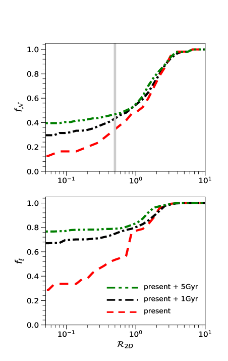
Figure 18: $f_{\scriptscriptstyle\mathcal{N}}$ (top panel), and $f_{\ell}$ (bottom panel), as a function of projected radius, at three different times into the future, assuming that all GCs survive against tidal disruption. The full sample of GCs was used. As a guide for the eye, the vertical line in the upper panel marks the radial distance $\mathcal{R}_{2\scriptscriptstyle\rm D}=0.5$.

In this context, the nucleation fraction should increase with time as GCs sink to the galaxy centre. From the observed current values of $M_{\scriptscriptstyle V,\rm GC}$ and $\mathcal{R}_{2\scriptscriptstyle\rm D}$ of the GCs in our sample, using our Monte Carlo model described in Section 4, we can predict the radial distribution of GCs at later times. Figure 18 shows $f_{\scriptscriptstyle\mathcal{N}}$ and $f_{\ell}$ at present time, at $1$ Gyr, and at $5$ Gyr from now. It was assumed again that the current 3D distance of the GCs are $\times\sqrt{3/2}$ their projected distance, and that all the GCs survive against tidal disruption for the next $5$ Gyr. The redistribution of the GCs inside one effective radius of the galaxies is apparent. Both profiles, $f_{\small\mathcal{N}}$ and $f_{\ell}$, flatten in the inner region because there dynamical friction is very efficient. The number of galaxies hosting a NSC will change from $6$ ($23\%$ of the dSph galaxies under study) at the present epoch to $16$ ($60\%$) in the next $1$ Gyr (see Figure 19). On the other hand, Figure 19 also shows that the number of GCs inside $\mathcal{R}_{2\scriptscriptstyle\rm D}=0.5$ decreases from $\mathcal{N}_{\Pi}=13$ to $4$ in the next $2$ Gyr. Since the present distribution of GCs evolves in a short timescale compared with the lifetime of the GCs, it would imply that we are living in a special time of their evolution. Cole et al. (2012) refers to this problem as the immediate timing problem. This timing problem is a different view of the problem of fine-tuning of the starting distances of the GCs.

7 Discussion

7.1 Eccentric orbits, tidal disruption of GCs, and tidal stripping of dark haloes

The results of the previous sections rely on various assumptions and simplifications. For all clusters, we have adopted circular orbits. Some of the GCs that are now located at $0<\mathcal{R}_{2\scriptscriptstyle\rm D}<0.5$ may have avoided strong orbital decay if they are on elongated orbits and they are now passing close to pericentre. Given that GCs in eccentric orbits spend a considerable fraction of the orbital time far from pericentre, the inclusion of eccentric orbits for outer GCs can alleviate slightly the tension between predictions and observations. In addition, if inner GCs are on elongated orbits, the problem is exacerbated because eccentric orbits have a shorter $\tau_{\scriptscriptstyle\rm DF}$ according to Arca-Sedda et al. (2015) formula (see Section 4).

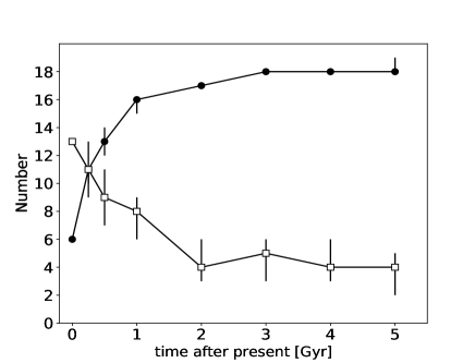
Figure 19: Number of galaxies with an NSC (filled circles) and $N_{\Pi}$ (empty squares) over the next $5$ Gyr, assuming that all GCs survive against tidal disruption. We have used the full sample of GCs.

We must stress that our Monte Carlo simulations do not include disruption of GCs by tidal forces. Because of the tidal dissolution of GCs, the current population of GCs is a fraction of the initial population. Given that the strength of the tidal forces on GCs in cuspy haloes increases as they sink towards the galactic centre, we would expect a depletion of GCs in the inner galaxy (e.g., Shao et al., 2021). Therefore, it seems challenging that the inclusion of tidal disruption of GCs can solve the offset in the value of $\mathcal{N}_{\Pi}$. Nevertheless, it could be interesting to start with a larger population of GCs and derive the final spatial distribution of GCs when tidal disruption is included.

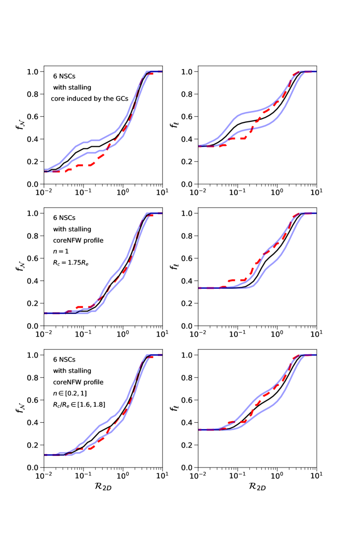
Figure 20: Comparison between the predicted distributions $f_{\scriptscriptstyle\mathcal{N}}$ and $f_{\scriptscriptstyle\ell}$ in cored dark matter haloes and those determined by observations. We assume that the inspiralling of GCs stalls at the radius $R_{\rm stall}$, which satisfies $R_{t}(R_{\rm stall})=R_{\rm stall}$, being $R_{t}$ the GC tidal radius. The tidal radius is computed using either the NFW profile or the coreNFW profile with parameters $n$ and $R_{c}$ as indicated in the left insets. The six central GCs are treated as ‘pure’ NSCs, i.e. it is assumed that they were born at the centre of the host galaxy. The distribution of starting radial distances of non-central GCs is given by Equation (4) as in our canonical model. Line colours and style codes are the same as those used in Figures 7, 8, 10, 11, and 13.

We have also ignored the effect of the tidal heating of the host galaxies by companion galaxies. Tidal stripping and shocking by neighbouring galaxies can lower the central dark matter density of the haloes of dSph galaxies (e.g., Battaglia et al., 2015; Genina et al., 2020). The values of the tidal index $\Theta$ in Table 1 indicate that tidal effects can be important for some dSph galaxies in our sample. In particular, And XXV has peculiar properties, which were interpreted as the result of tides (Collins et al., 2013). The strength of tidal fields depends on the pericentre of the dSph’s orbits around the host galaxy, which is unknown for most of the galaxies in our sample. In the case of Fornax, tidal stirring has been considered by other authors and their effects seem to not alter significantly the orbital decay of its GCs (Oh, Lin & Richer, 2000; Arca-Sedda & Capuzzo-Dolcetta, 2016; Borukhovetskaya et al., 2021). Nonetheless, these issues warrant more attention in future work.

7.2 Core stalling as a solution to the timing problem

The timing problem (or fine-tuning problem) could be interpreted as indications of the breakdown of the NFW profile at small radii. Indeed, GCs themshelves can tidally dirupt the dark halo cusp, transforming it into a core, when the sinking GCs are close to the galaxy centre (Goerdt et al., 2010). This transformation occurs when the orbital radius of the GC is comparable to its tidal radius. When a core is formed, dynamical friction is suppressed and GCs stall. Goerdt et al. (2010) were able to empirically derive the core-stalling radius in terms of the distance at which the mass of the satellite equals the enclosed mass of the host galaxy. However, Petts, Read & Gualandris (2016) find a more simple prescription for core-stalling in terms of the tidal radius of the GC; core-stalling happens at a radius $R_{\rm stall}$ given by

$$R_{t}(R_{\rm stall})=R_{\rm stall},$$ (6)

where

$$R_{t}^{3}=\frac{GM_{\rm\scriptscriptstyle GC}}{\Omega^{2}-d^{2}\Phi/dr^{2}},$$ (7)

with $\Phi$ the gravitational potential of the host galaxy and $\Omega$ the angular velocity of a test particle in circular orbit, both evaluated at the instantaneous orbital radius of the GC.

We have explored how $f_{\scriptscriptstyle\mathcal{N}}$ and $f_{\ell}$ are modified in this scenario as follows. We assume that the host galaxies follow an NFW profile before cusp-core transformation, with the halo parameters as described in Section 4. Then, for each host galaxy, we know $\Omega(r)$ and $d^{2}\Phi/dr^{2}$. For each non-central GC and its host galaxy, we determine $R_{\rm stall}$ by solving Equation (6). Finally, when computing the model distributions, we switch off dynamical friction at $R_{\rm stall}$. For the specific six GCs that are observed at the centre of the host galaxy (see Section 5.2), we assume that they were formed at the galaxy centres, i.e. they are pure NSCs ($\mathcal{R}_{3\rm\scriptscriptstyle D}=0$ at any time). Otherwise, this scenario would predict that no GC could lie in the centres of galaxies, as they would always halt their migration at $R_{\rm stall}$.

The top panels in Figure 20 show the results. By construction, the values of $f_{\scriptscriptstyle\mathcal{N}}(0)$ and $f_{\ell}(0)$ match the observed values because of the assumption that NSCs should have been formed at $r=0$. The inclusion of core-stalling leads to steeper profiles inside $0.1R_{e}$, which reflects the fact that typically $R_{\rm stall}\lesssim 0.1R_{e}$ in our sample. However, the observed profiles are almost flat in that region. In fact, the cores formed by the GCs in their own are too small to satisfactorily account for the observed mean abundance and luminosity of GCs between $0.1R_{e}$ and $0.7R_{e}$. Almost identical diagrams are obtained if instead of the condition $R_{t}(R_{\rm stall})=R_{\rm stall}$, we assume that stalling occurs at a radius where the enclosed mass is comparable to the GC mass (not shown).

It has been suggested that gravitational potential fluctuations, created by gas outflows driven by bursty star formation and episodes of gas inflows, could be a viable mechanism to transform cusps into cores (e.g., Pontzen & Governato, 2012; Read et al., 2016; Lazar et al., 2020). Core formation can also be driven by angular momentum transfer between dark matter particles and cold gas clumps (El-Zant et al., 2001; Nipoti & Binney, 2015), or through impulsive heating from minor mergers (Orkney et al., 2021). Other scenarios for core formation are based on modifications to the dark matter physics (e.g., Davé et al., 2001; Sánchez-Salcedo, 2003; Schive et al., 2014).

Figure 20 shows the expected radial distributions using the “coreNFW” profile from Read et al. (2016) for all the galaxies in the sample. The coreNFW profile is a modified NFW profile which was found to describe the simulated dark haloes in dwarf galaxies after including stellar feedback. The model is parameterised by the size of the dark halo core $R_{c}$ and the power-law slope of the core $0\leq n\leq 1$, where $n=0$ corresponds to the cuspy NFW profile and $n=1$ produces a flat dark matter core. As before, the stalling radius is computed by solving the Equation (6).

We find good agreement between the predicted and the observed distributions when we set $n$ to $1$ and $R_{c}$ to $1.75R_{e}$, as suggested by Read et al. (2016). We also show the results in a case where $n$ is uniformly sampled between $0.2$ and $1$, and $R_{c}$ between $1.6R_{e}$ and $1.8R_{e}$. The agreement between the observed and the predicted profiles is reasonable. Therefore, the hypothesis that the dark haloes of dSph galaxies have cores of size $\sim R_{e}$ is a natural solution for the timing problem; both the low fraction of central GCs and the high fraction of off-centre GCs inside $0.5R_{e}$ could be a consequence of the reduction of dynamical friction inside the cores. Note, however, that dark matter cores of size comparable to $\sim R_{e}$ can form only if star formation proceeds for several Gyr (Read et al., 2016), and star formation is bursty enough to prevent that subsequent gas accretion reforms a cusp (Benítez-Llambay et al., 2019).

8 Conclusions

In this paper, we have collected from the literature a sample of GCs hosted by low-luminosity spheroidal galaxies, in order to investigate the role of dynamical friction in the spatial distribution of the GCs in these galaxies. Firstly, we have searched for any statistical evidence of mass segregation in the stacked distribution of GCs. We have found a moderate correlation between specific luminosity ($\ell$) and the projected distance of the GCs to the centre of the host galaxy in units of the core radius ($\mathcal{R}_{2\scriptscriptstyle\rm D}$), with a high significance level.

We have performed simple Monte Carlo simulations to predict the radial distribution of the number and luminosity of the GCs, assuming that their orbital evolution is driven by dynamical friction with the dark matter. If all dSph galaxies in our sample have an NFW dark halo, the predicted number of non-nuclear GCs inside one half effective radius ($\mathcal{N}_{\Pi}$) is considerably smaller than observed (see Figure 9). In the models, $\mathcal{N}_{\Pi}$ is low because GCs spend little time in that inner region given that the timescale to sink is very short. Therefore, the timing problem of the orbital decay of GCs is not exclusive of the Fornax dSph galaxy.

The timing problem is equivalent to invoke a fine-tuning in the starting radii of the GCs. In fact, it is always possible to find the starting distance of the GCs if we know the final orbital radii and the halo parameters (see Figure 15), but relatively small changes in the starting distances lead to very different final orbital radii.

A third view of the timing problem is the “immediate timing problem” (Cole et al., 2012). Using our probabilistic approach and the observed present-day GC projected distances, we have predicted the future radial distribution of GCs, assuming that all GCs survive against tidal dissolution (see Figure 18). While at the present-day, about $\sim 23\%$ (6/26) of the galaxies in our sample has a central GC, this fraction will change to becoming $\sim 60\%$ (16/26) in the next $1$ Gyr. In addition, the value of $\mathcal{N}_{\Pi}$ will change from $13$ at present-day to $4$ at $2$ Gyr into the future.

The timing problem is alleviated if, instead of an NFW profile, one considers weakly cuspy haloes or cored haloes. In particular, the present-day GC distribution can be accounted for if dark haloes have cores of size $\sim R_{e}$ (see Figure 20). Several mechanisms have been suggested that could transform cusps into cores. Thus, the possibility that the NFW profile breaks down at small radii in dSph galaxies seems plausible. It is less clear whether gas outflows/inflows can develop cores of that size.

Studies including the internal dynamics and the survival of GCs may provide additional constraints on the dark matter profile (e.g., Amorisco, 2017; Contenta et al., 2018; Orkney et al., 2019; Leaman et al., 2020). Moreover, new data of the distribution of GC candidates around early-type dwarf galaxies (e.g., Carlsten et al., 2021) could significantly increase the statistics for studying the inspiralling of GCs and the role of dynamical friction. This investigation is planned for future work.

Data Availability

No new data were generated or analysed in support of this research.

References

- Amorisco (2017) Amorisco N. C. 2017, ApJ, 844, 64
- Amorisco & Evans (2012) Amorisco N. C., Evans N. W. 2012, MNRAS, 419, 184
- Angus & Diaferio (2009) Angus G. W., Diaferio A. 2009, MNRAS, 396, 887
- Antonini et al. (2012) Antonini F., Capuzzo-Dolcetta R., Mastrobuono-Battisti A., Merritt, D. 2012, ApJ, 750, 111
- Arca-Sedda et al. (2014) Arca-Sedda M., Capuzzo-Dolcetta R. 2014, ApJ, 785, 51
- Arca-Sedda et al. (2015) Arca-Sedda M., Capuzzo-Dolcetta R., Antonini F., Seth A. 2015, ApJ, 806, 220
- Arca-Sedda & Capuzzo-Dolcetta (2016) Arca-Sedda M., Capuzzo-Dolcetta R. 2016, MNRAS, 461, 4335
- Bar et al. (2021) Bar N., Blas D., Blum K., Kim H. 2021, Phys. Rev. D, 104, 043021
- Battaglia et al. (2015) Battaglia G., Sollima A., Nipoti C. 2015, MNRAS, 454, 2401
- Beasley et al. (2019) Beasley M. A., Leaman R., Gallart C., Larsen S. S., Battaglia G., Monelli M., Pedreros M. H. 2019, MNRAS, 487, 1986
- Bellazzini et al. (2014) Bellazzini M., Beccari G., Fraternali F. et al. 2014, A&A, 566, A44
- Benítez-Llambay et al. (2019) Benítez-Llambay A., Frenk C. A., Ludlow A. D., Navarro J. F. 2019, MNRAS, 488, 2387
- Boldrini et al. (2019) Boldrini P., Mohayaee R., Silk J. 2019, MNRAS, 485, 2546
- Borukhovetskaya et al. (2021) Borukhovetskaya A., Errani R., Navarro J. F., Fattahi A., Santos-Santos I. 2021, arXiv:2104.00011
- Caldwell et al. (1998) Caldwell N., Armandroff T. E., Da Costa G. S., Seitzer P. 1998, AJ, 115, 535
- Caldwell et al. (2017) Caldwell N., Strader J., Sand D. J., Willman B., Seth A. C. 2017, PASA, 34, e039
- Capuzzo-Dolcetta & Miocchi (2008) Capuzzo-Dolcetta R., Miocchi P. 2008, ApJ, 681, 1136
- Capuzzo-Dolcetta & Donnarumma (2001) Capuzzo-Dolcetta R., Donnarumma I. 2001, MNRAS, 328, 645
- Capuzzo-Dolcetta & Tesseri (1999) Capuzzo-Dolcetta R., Tesseri A. 1999, MNRAS, 308, 961
- Carlsten et al. (2021) Carlsten S. G., Greene J. E., Beaton R. L., Greco J. P. 2021, arXiv:2105.03440
- Chiboucas et al. (2009) Chiboucas K., Karachentsev I. D., Tully R. B. 2009, AJ, 137, 3009
- Cole et al. (2012) Cole D. R., Dehnen W., Read J. I., Wilkinson M. I. 2012, MNRAS, 426, 601
- Cole et al. (2017) Cole A. A., Weisz D. R., Skillman E. D. et al. 2017, ApJ, 837, 54
- Coleman et al. (2004) Coleman M. G., Da Costa G. S., Bland-Hawthorn J., et al. 2004, AJ, 127, 832
- Collins et al. (2013) Collins M. L. M., Chapman S. C., Rich R. M. et al. 2013, ApJ, 768, 172
- Contenta et al. (2018) Contenta F., Balbinot E., Petts J. A. et al. 2018, MNRAS, 476, 3124
- Crnojević et al. (2016) Crnojević D., Sand D. J., Zaritsky D., Spekkens K., Willman B., Hargis J. R. 2016, ApJ, 824, L14
- Cusano et al. (2016) Cusano F., Garofalo A., Clementini G., et al. 2016, ApJ, 829, 26
- Curran (2015) Curran P. A. 2015, arXiv:1411.3816
- Da Costa et al. (2009) Da Costa G. S., Grebel E. K., Jerjen H., Rejkuba M., Sharina E. 2009, AJ, 137, 4361
- de Boer & Fraser (2016) de Boer T. J. L., Fraser M. 2016, A&A, 590, A35
- de Swardt et al. (2010) de Swardt B., Kraan-Korteweg R. C., Jerjen H. 2010, MNRAS, 407, 955
- den Brok et al. (2014) den Brok M., Peletier R. F., Seth A. et al. 2014, MNRAS, 445, 2385
- Davé et al. (2001) Davé R., Spergel D. N., Steinhardt P. J., Wandelt B. D., 2001, ApJ, 547, 574
- Dutton & Macciò (2014) Dutton A. A., Macciò A. V. 2014, MNRAS, 441, 3359
- El-Zant et al. (2001) El-Zant A., Shlosman I., Hoffman Y. 2001, ApJ, 560, 636
- Elmegreen & Efremov (1997) Elmegreen B. G., Efremov Y. N. 1997, ApJ, 480, 235
- Errani et al. (2018) Errani R., Peñarrubia J., Walker M. G. 2018, MNRAS, 481, 5073
- Fahrion et al. (2020) Fahrion K., Muller O., Rejkuba M., et al. 2020, A&A, 634, A53
- Forbes et al. (2018) Forbes D. A., Read J. I., Gieles M., Collins M. L. M. 2018, MNRAS, 481, 5592
- Forbes & Remus (2018) Forbes D. A., Remus R.-S. 2018, MNRAS, 479, 4760
- Gebhardt et al. (1996) Gebhardt K., Richstone D., Ajhar E. A. et al. 1996, AJ, 112, 105
- Genina et al. (2018) Genina A., Benítez-Llambay A., Frenk, C. S. et al. 2018, MNRAS, 474, 1398
- Genina et al. (2020) Genina A., Read J. I., Fattahi A., Frenk C. S. 2020, arXiv:2011.09482
- Georgiev et al. (2009) Georgiev I. Y., Hilker M., Puzia T. H., Goudfrooij P., Baumgardt H. 2009, MNRAS, 396, 1075
- Georgiev et al. (2010) Georgiev I. Y., Puzia T. H., Goudfrooij P., Hilker M. 2010, MNRAS, 406, 1967
- Gnedin et al. (2014) Gnedin O. Y., Ostriker J. P., Tremaine S. 2014, ApJ, 785, 71
- Goerdt et al. (2006) Goerdt T., Moore B., Read J. I., Stadel J., Zemp M. 2006, MNRAS, 368, 1073
- Goerdt et al. (2010) Goerdt T., Moore B., Read J. I., Stadel, J. 2010, ApJ, 725, 1707
- Gualandris & Merrit (2008) Gualandris A., Merrit D. 2008, ApJ, 678, 780
- Guo et al. (2010) Guo Q., White S. D. M., Li C., Boylan-Kolchin M. 2010, MNRAS, 404, 1111
- Hayashi et al. (2020) Hayashi K., Chiba M., Ishiyama T. 2020, MNRAS, 904, 45
- Hoyer et al. (2021) Hoyer N., Neumayer N., Georgiev I. Y., Seth A., Greene J. E. 2021, MNRAS, 507, 3246
- Inoue (2009) Inoue S. 2009, MNRAS, 397, 709
- Jardel & Gebhardt (2013) Jardel J. R., Gebhardt K. 2013, ApJ, 775, L30
- Jardel et al. (2013) Jardel J. R., Gebhardt K., Fabricius M. H., Drory N., Williams M. J. 2013, ApJ, 793, 91
- Karachentsev et al. (2000) Karachentsev I. D., Karachentseva V. E., Dolphin A. E., et al. 2000, A&A, 363, 117
- Karachentsev et al. (2004) Karachentsev I. D., Karachentseva V. E., Huchtmeier W. K., Makarov D. I. 2004, AJ, 127, 2031
- Karachentsev et al. (2015) Karachentsev I. D., Kniazev A. Yu., Sharina M. E. 2015, Astronomische Nachrichten, 336, 707
- Kirby et al. (2014) Kirby E. N., Bullock J. S., Boylan-Kolchin M., Kaplinghat M., Cohen J. G. 2014, MNRAS, 439, 1015
- Kruijssen (2012) Kruijssen J. M. D. 2012, MNRAS, 426, 3008
- Kruijssen (2014) Kruijssen J. M. D. 2014, CQGra, 31, 244006
- Lahén et al. (2019) Lahén N., Naab T., Johansson P. H., Elmegreen B., Hu C.-Y., Walch S. 2019, ApJ, 879, L18
- Lazar et al. (2020) Lazar A., Bullock J. S., Boylan-Kolchin M. et al. 2020 MNRAS, 497, 2393
- Leaman et al. (2020) Leaman R., Ruiz-Lara T., Cole A. A., et al. 2020, MNRAS, 492, 5102
- Leung et al. (2020) Leung G. Y. C., Leaman R., van de Ven G., Battaglia G. 2020, MNRAS, 493, 320
- Lianou et al. (2010) Lianou S., Grebel E. K., Koch A. 2010, A&A, 521, A43
- Lotz et al. (2001) Lotz J. M., Telford R., Ferguson H. C., Miller B. W., Stiavelli M., Mack J. 2001, ApJ, 552, 572
- Ludlow et al. (2016) Ludlow A. D., Bose S., Angulo R. E. et al. 2016, MNRAS, 460, 1214
- Makarova et al. (2010) Makarova L., Koleva M., Makarov D., Prugniel P. 2010, MNRAS, 406, 1152
- Maraston (2005) Maraston C. 2005, MNRAS, 362, 799
- Massari et al. (2018) Massari D., Breddels M. A., Helmi A., Posti L., Brown A. G. A., Tolstoy E. 2018, Nature Astronomy, 2, 156
- Massari et al. (2020) Massari D., Helmi A., Mucciarelli A., Sales L. V., Spina L., Tolstoy E. 2020, A&A, 633, A36
- McConnachie (2012) McConnachie A. W. 2012, AJ, 144, 4
- McLaughlin & van der Marel (2005) McLaughlin D. E., van der Marel R. P. 2005, ApJS, 161, 304
- Meadows et al. (2020) Meadows N., Navarro J. F., Santos-Santos I., Benítez-Llambay A., Frenk C. 2020, MNRAS, 491, 3336
- Nipoti & Binney (2015) Nipoti C., Binney J. 2015, MNRAS, 446, 1820
- Oh, Lin & Richer (2000) Oh K. S., Lin D. N. C., Richer H. B. 2000, ApJ, 531, 727
- Orkney et al. (2019) Orkney M. D. A., Read J. I., Petts J. A., Gieles M. 2019, MNRAS, 488, 2977
- Orkney et al. (2021) Orkney M. D. A., Read J. I., Rey M. P. et al. 2021, MNRAS, 504, 3509
- Pascale et al. (2018) Pascale R., Posti L., Nipoti C., Binney J. 2018, MNRAS, 480, 927
- Petts, Read & Gualandris (2016) Petts J. A., Read J. I., Gualandris A. 2016, MNRAS, 463, 858
- Pontzen & Governato (2012) Pontzen A., Governato F. 2012, MNRAS, 421, 3464
- Puzia & Sharina (2008) Puzia T. H., Sharina M. E. 2008, ApJ, 674, 909
- Read et al. (2016) Read J. I., Agertz O., Collins M. L. M. 2016, MNRAS, 459, 2573
- Read et al. (2017) Read J. I., Iorio G., Agertz O., Fraternali F. 2017, MNRAS, 467, 2019
- Read et al. (2018) Read J. I., Walker M. G., Steger P. 2018, MNRAS, 481, 860
- Read et al. (2019) Read J. I., Walker M. G., Steger P. 2019, MNRAS, 484, 1401
- Richardson & Fairbairn (2014) Richardson T., Fairbairn M. 2014, MNRAS, 441, 1584
- Sánchez-Janssen et al. (2019) Sánchez-Janssen R., Côté P., Ferrarese L., et al. 2019, ApJ, 878, 18
- Sánchez-Salcedo (2003) Sánchez-Salcedo F. J. 2003, ApJ, 591, L107
- Sánchez-Salcedo et al. (2006) Sánchez-Salcedo F. J., Reyes-Iturbide J., Hernandez X. 2006, MNRAS, 370, 1829
- Schive et al. (2014) Schive H.-Y., Chiueh T., Broadhurst T. 2014, Nature Physics, 10, 496
- Shao et al. (2021) Shao S., Cautun M., Frenk C. S., Reina-Campos M., Deason A. J., Crain R. A., Kruijssen J. M. D., Pfeffer J. 2021, MNRAS, 507, 2339
- Sharina et al. (2010) Sharina M. E., Chandar R., Puzia T. H., Goudfrooij P., Davoust E. 2010, MNRAS, 405, 839
- Sharina et al. (2008) Sharina M. E., Karachentsev I. D., Dolphin A. E. et al. 2008, MNRAS, 384, 1544
- Sharina et al. (2005) Sharina M. E., Puzia T. H., Makarov D. I. 2005, A&A, 442, 85
- Sharina et al. (2017) Sharina M. E., Shimansky V. V., Kniazev A. Y. 2017, MNRAS, 471, 1955
- Sharina et al. (2003) Sharina M. E., Sil’chenko O. K., Burenkov A. N. 2003, A&A, 397, 831
- Simon et al. (2021) Simon J. D., Brown T. M., Drlica-Wagner A., et al. 2021, ApJ, 908, 18
- Strigari et al. (2018) Strigari L. E., Frenk C. S., White S. D. M. 2018, ApJ, 860, 56
- Tremaine (1976) Tremaine S. D. 1976, ApJ, 203, 345
- Tremaine et al. (1975) Tremaine S. D., Ostriker J. P., Spitzer L. Jr 1975, ApJ, 196, 407
- Tudorica et al. (2015) Tudorica A., Georgiev I. Y., Chies-Santos A. L. 2015, A&A, 581, A84
- Turner et al. (2012) Turner M. L., Côté P., Ferrarese L., Jordán A., Blakeslee J. P., Mei S., Peng E. W., West M. J. 2012, ApJ, 203, 5
- Walker & Peñarrubia (2011) Walker M. G., Peñarrubia J. 2011, ApJ, 742, 20