Context Uncertainty in Contextual Bandits
with Applications to Recommender Systems
Abstract
Recurrent neural networks have proven effective in modeling sequential user feedbacks for recommender systems. However, they usually focus solely on item relevance and fail to effectively explore diverse items for users, therefore harming the system performance in the long run. To address this problem, we propose a new type of recurrent neural networks, dubbed recurrent exploration networks (REN), to jointly perform representation learning and effective exploration in the latent space. REN tries to balance relevance and exploration while taking into account the uncertainty in the representations. Our theoretical analysis shows that REN can preserve the rate-optimal sublinear regret even when there exists uncertainty in the learned representations. Our empirical study demonstrates that REN can achieve satisfactory long-term rewards on both synthetic and real-world recommendation datasets, outperforming state-of-the-art models.
Introduction
Modeling and predicting sequential user feedbacks is a core problem in modern e-commerce recommender systems. In this regard, recurrent neural networks (RNN) have shown great promise since they can naturally handle sequential data (Hidasi et al. 2016; Quadrana et al. 2017; Belletti, Chen, and Chi 2019; Ma et al. 2020). While these RNN-based models can effectively learn representations in the latent space to achieve satisfactory immediate recommendation accuracy, they typically focus solely on relevance and fall short of effective exploration in the latent space, leading to poor performance in the long run. For example, a recommender system may keep recommending action movies to a user once it learns that she likes such movies. This may increase immediate rewards, but the lack of exploration in other movie genres can certainly be detrimental to long-term rewards.
So, how does one effectively explore diverse items for users while retaining the representation power offered by RNN-based recommenders. We note that the learned representations in the latent space are crucial for these models’ success. Therefore we propose recurrent exploration networks (REN) to explore diverse items in the latent space learned by RNN-based models. REN tries to balance relevance and exploration during recommendations using the learned representations.
One roadblock is that effective exploration relies heavily on well learned representations, which in turn require sufficient exploration; this is a chicken-and-egg problem. In a case where RNN learns unreasonable representations (e.g., all items have the same representations), exploration in the latent space is meaningless. To address this problem, we enable REN to take into account the uncertainty of the learned representations as well during recommendations. Essentially items whose representations have higher uncertainty can be explored more often. Such a model can be seen as a contextual bandit algorithm that is aware of the uncertainty for each context. Our contributions are as follows:
-
1.
We propose REN as a new type of RNN to balance relevance and exploration during recommendation, yielding satisfactory long-term rewards.
-
2.
Our theoretical analysis shows that there is an upper confidence bound related to uncertainty in learned representations. With such a bound implemented in the algorithm, REN can achieve the same rate-optimal sublinear regret. To the best of our knowledge, we are the first to study the regret bounds under “context uncertainty”.
-
3.
Experiments of joint learning and exploration on both synthetic and real-world temporal datasets show that REN significantly improve long-term rewards over state-of-the-art RNN-based recommenders.
Related Work
Deep Learning for Recommender Systems. Deep learning (DL) has been playing a key role in modern recommender systems (Salakhutdinov, Mnih, and Hinton 2007; van den Oord, Dieleman, and Schrauwen 2013; Wang, Wang, and Yeung 2015; Wang, Shi, and Yeung 2015, 2016; Li and She 2017; Chen et al. 2019; Fang et al. 2019; Tang et al. 2019; Ding et al. 2021; Gupta et al. 2021). (Salakhutdinov, Mnih, and Hinton 2007) uses restricted Boltzmann machine to perform collaborative filtering in recommender systems. Collaborative deep learning (CDL) (Wang, Wang, and Yeung 2015; Wang, Shi, and Yeung 2016; Li and She 2017) is devised as Bayesian deep learning models (Wang and Yeung 2016, 2020; Wang 2017) to significantly improve recommendation performance. In terms of sequential (or session-based) recommender systems (Hidasi et al. 2016; Quadrana et al. 2017; Bai, Kolter, and Koltun 2018; Li et al. 2017; Liu et al. 2018; Wu et al. 2019; Ma et al. 2020), GRU4Rec (Hidasi et al. 2016) was first proposed to use gated recurrent units (GRU) (Cho et al. 2014), an RNN variant with gating mechanism, for recommendation. Since then, follow-up works such as hierarchical GRU (Quadrana et al. 2017), temporal convolutional networks (TCN) (Bai, Kolter, and Koltun 2018), and hierarchical RNN (HRNN) (Ma et al. 2020) have tried to achieve improvement in accuracy with the help of cross-session information (Quadrana et al. 2017), causal convolutions (Bai, Kolter, and Koltun 2018), as well as control signals (Ma et al. 2020). We note that our REN does not assume specific RNN architectures (e.g., GRU or TCN) and is therefore compatible with different RNN-based (or more generally DL-based) models, as shown in later sections.
Contextual Bandits. Contextual bandit algorithms such as LinUCB (Li et al. 2010) and its variants (Yue and Guestrin 2011; Agarwal et al. 2014; Li, Karatzoglou, and Gentile 2016; Kveton et al. 2017; Foster et al. 2018; Korda, Szorenyi, and Li 2016; Mahadik et al. 2020; Zhou, Li, and Gu 2019) have been proposed to tackle the exploitation-exploration trade-off in recommender systems and successfully improve upon context-free bandit algorithms (Auer 2002). Similar to (Auer 2002), theoretical analysis shows that LinUCB variants could achieve a rate-optimal regret bound (Chu et al. 2011). However, these methods either assume observed context (Zhou, Li, and Gu 2019) or are incompatible with neural networks (Li, Karatzoglou, and Gentile 2016; Yue and Guestrin 2011). In contrast, REN as a contextual bandit algorithm runs in the latent space and assumes user models based on RNN; therefore it is compatible with state-of-the-art RNN-based recommender systems.
Diversity-Inducing Models. Various works have focused on inducing diversity in recommender systems (Nguyen et al. 2014; Antikacioglu and Ravi 2017; Wilhelm et al. 2018; Bello et al. 2018). Usually such a system consists of a submodular function, which measures the diversity among items, and a relevance prediction model, which predicts relevance between users and items. Examples of submodular functions include the probabilistic coverage function (Hiranandani et al. 2019) and facility location diversity (FILD) (Tschiatschek, Djolonga, and Krause 2016), while relevance prediction models can be Gaussian processes (Vanchinathan et al. 2014), linear regression (Yue and Guestrin 2011), etc. These models typically focus on improving diversity among recommended items in a slate at the cost of accuracy. In contrast, REN’s goal is to optimize for long-term rewards through improving diversity between previous and recommended items. We include some slate generation in our real-data experiments for completeness.
Recurrent Exploration Networks
In this section we first describe the general notations and how RNN can be used for recommendation, briefly review determinantal point processes (DPP) as a diversity-inducing model as well as their connection to exploration in contextual bandits, and then introduce our proposed REN framework.
Notation and RNN-Based Recommender Systems
Notation. We consider the problem of sequential recommendations where the goal is to predict the item a user interacts with (e.g., click or purchase) at time , denoted as , given her previous interaction history . Here is the index for the item at time , is a one-hot vector indicating an item, and is the number of total items. We denote the item embedding (encoding) for as , where is the encoder as a part of the RNN. Correspondingly we have . Strictly speaking, in an online setting where the model updates at every time step , also changes over time; in Sec. Recurrent Exploration Networks we use as a shorthand for for simplicity. We use to denote the norm, where the superscript means the -th entry of the vector
RNN-Based Recommender Systems. Given the interaction history , the RNN generates the user embedding at time t as , where , and is the recurrent part of the RNN. Assuming tied weights, the score for each candidate item is then computed as . As the last step, the recommender system will recommend the items with the highest scores to the user. Note that the subscript indexes the items, and is equivalent to an ‘action’, usually denoted as , in the context of bandit algorithms.
Determinantal Point Processes for Diversity and Exploration
Determinantal point processes (DPP) consider an item selection problem where each item is represented by a feature vector . Diversity is achieved by picking a subset of items to cover the maximum volume spanned by the items, measured by the log-determinant of the corresponding kernel matrix, , where is included to prevent singularity. Intuitively, DPP penalizes colinearity, which is an indicator that the topics of one item are already covered by the other topics in the full set. The log-determinant of a kernel matrix is also a submodular function (Friedland and Gaubert 2013), which implies a -optimal guarantees from greedy solutions. The greedy algorithm for DPP via the matrix determinant lemma is
| (1) | ||||
| (2) | ||||
| (3) |
Interestingly, note that has the same form as the confidence interval in LinUCB (Li et al. 2010), a commonly used contextual bandit algorithm to boost exploration and achieve long-term rewards, suggesting a connection between diversity and long-term rewards (Yue and Guestrin 2011). Intuitively, this makes sense in recommender systems since encouraging diversity relative to user history (as well as diversity in a slate of recommendations in our experiments) naturally explores user interest previously unknown to the model, leading to much higher long-term rewards, as shown in Sec. Experiments.
Recurrent Exploration Networks
Exploration Term. Based on the intuition above, we can modify the user-item score to include a diversity (exploration) term, leading to the new score
| (4) |
where the first term is the relevance score and the second term is the exploration score (measuring diversity between previous and recommended items). is RNN’s hidden states at time representing the user embedding. The hyperparameter aims to balance two terms.
Uncertainty Term for Context Uncertainty. At first blush, given the user history the system using Eqn. 4 will recommend items that are (1) relevant to the user’s interest and (2) diverse from the user’s previous items. However, this only works when item embeddings are correctly learned. Unfortunately, the quality of learned item embeddings, in turn, relies heavily on the effectiveness of exploration, leading to a chicken-and-egg problem. To address this problem, one also needs to consider the uncertainty of the learned item embeddings. Assuming the item embedding , where , we have the final score for REN:
| (5) |
where and . The term quantifies the uncertainty for each dimension of , meaning that items whose embeddings REN is uncertain about are more likely to be recommended. Therefore with the third term, REN can naturally balance among relevance, diversity (relative to user history), and uncertainty during exploration.
Putting It All Together. Algorithm 1 shows the overview of REN. Note that the difference between REN and traditional RNN-based recommenders is only in the inference stage. During training (Line 1 of Algorithm 1), one can train REN only with the relevance term using models such as GRU4Rec and HRNN. In the experiments, we use uncertainty estimates , where is item ’s total number of impressions (i.e., the number of times item has been recommended) for all users. The intuition is that: the more frequently item is recommended, the more frequently its embedding gets updated, the faster decreases.111There are some caveats in general. assumes that all coordinates of shrink at the same rate. However, REN exploration mechanism associates with the total variance of the features of an item. This may not ensure all feature dimensions to be equally explored. See (Jun et al. 2019) for a different algorithm that analyzes the exploration of the low-rank feature space. Our preliminary experiments show that does decrease at the rate of , meaning that the assumption in Lemma 10 is satisfied. From the Bayesian perspective, may not accurately reflect the uncertainty of the learned , which is a limitation of our model. In principle, one can learn from data using the reparameterization trick (Kingma and Welling 2014) with a Gaussian prior on and examine whether the assumption in Lemma 10; this would be interesting future work.
Linearity in REN. REN only needs a linear bandit model; REN’s output is linear w.r.t. and . Note that NeuralUCB (Zhou, Li, and Gu 2019) is a powerful nonlinear extension of LinUCB, i.e., its output is nonlinear w.r.t. and . Extending REN’s output from to a nonlinear function as in NeuralUCB is also interesting future work.222In other words, we did not fully explain why could be shared between non-linear RNN and the uncertainty bounds based on linear models. On the other hand, we did observe promising empirical results, which may encourage interested readers to dive deep into different theoretical analyses.
Beyond RNN. Note that our methods and theory go beyond RNN-based models and can be naturally extended to any latent factor models including transformers, MLPs, and matrix factorization. The key is the user embedding , which can be instantiated with an RNN, a transformer, or a matrix-factorization model.
Theoretical Analysis
With REN’s connection to contextual bandits, we can prove that with proper and , Eqn. 5 is actually the upper confidence bound that leads to long-term rewards with a rate-optimal regret bound.
Reward Uncertainty versus Context Uncertainty. Note that unlike existing works which primarily consider the randomness from the reward, we take into consideration the uncertainty resulted from the context (content) (Mi et al. 2019; Wang, Xingjian, and Yeung 2016), i.e., context uncertainty. In CDL (Wang, Wang, and Yeung 2015; Wang, Shi, and Yeung 2016), it is shown that such content information is crucial in DL-based RecSys (Wang, Wang, and Yeung 2015; Wang, Shi, and Yeung 2016), and so is the associated uncertainty. More specifically, existing works assume deterministic and only assume randomness in the reward, i.e., they assume that , and therefore ’s randomness is independent of . The problem with this formulation is that they assume is deterministic and therefore the model only has a point estimate of the item embedding , but does not have uncertainty estimation for such . We find that such uncertainty estimation is crucial for exploration; if the model is uncertain about , it can then explore more on the corresponding item.
To facilitate analysis, we follow common practice (Auer 2002; Chu et al. 2011) to divide the procedure of REN into “BaseREN" (Algorithm 3) and “SupREN" stages correspondingly. Essentially SupREN introduces levels of elimination (with as an index) to filter out low-quality items and ensures that the assumption holds (see the Supplement for details of SupREN).
In this section, we first provide a high probability bound for BaseREN with uncertain embeddings (context), and derive an upper bound for the regret. As mentioned in Sec. Notation and RNN-Based Recommender Systems, for the online setting where the model updates at every time step , also changes over time. Therefore in this section we use , , , and in place of , , , and from Sec. Recurrent Exploration Networks to be rigorous.
Assumption 1.
Assume there exists an optimal , with , and such that . Further assume that there is an effective distribution such that where . Thus, the true underlying context is unavailable, but we are aided with the knowledge that it is generated by a multivariate normal with known parameters333Here we omit the identifiability issue of and assume that there is a unique for clarity. .
Upper Confidence Bound for Uncertain Embeddings
For simplicity denote the item embedding (context) as , where indexes the rounds (time steps) and indexes the items. We define:
| (6) |
where is the collected user feedback. Lemma 6 below shows that with and , Eqn. 5 is the upper confidence bound with high probability, meaning that Eqn. 5 upper bounds the true reward with high probability, which makes it a reasonable score for recommendations.
Lemma 1 (Confidence Bound).
With probability at least , we have for all that
where is the norm.
The proof is in the Supplement. This upper confidence bound above provides important insight on why Eqn. 5 is reasonable as a final score to select items in Algorithm 1 as well as the choice of hyperparameters and .
RNN to Estimate . REN uses RNN to approximate (useful in the proof of Lemma 6) in Eqn. 6. Note that a linear RNN with tied weights and a single time step is equivalent to linear regression (LR); therefore RNN is a more general model to estimate . Compared to LR, RNN-based recommenders can naturally incorporate new user history by incrementally updating the hidden states ( in REN), without the need to solve a linear equation. Interestingly, one can also see RNN’s recurrent computation as a simulation (approximation) for solving equations via iterative updating.
Regret Bound
Lemma 6 above provides an estimate of the reward’s upper bound at time . Based on this estimate, one natural next step is to analyze the regret after all rounds. Formally, we define the regret of the algorithm after rounds as
| (7) |
where is the optimal item (action) at round that maximizes , and is the action chose by the algorithm at round . Similar to (Auer 2002), SupREN calls BaseREN as a sub-routine. In this subsection, we derive the regret bound for SupREN with uncertain item embeddings.
Lemma 2.
With probability , for any and any , we have: (1) for any , (2) , and (3) for any .
Lemma 3.
In BaseREN, we have:
Lemma 4.
Assuming and for any and , then for any , we have the upper bound:
Essentially Lemma 8 links the regret to the width of the confidence bound (Line 3 of Algorithm 3 or the last two terms of Eqn. 5). Lemma 9 and Lemma 10 then connect to , which is sublinear in ; this is the key to achieve a sublinear regret bound. Note that is defined inside Algorithm 2 (SupREN) of the Supplement.
Interestingly, Lemma 10 states that the uncertainty only needs to decrease at the rate , which is consistent with our choice of in Sec. Recurrent Exploration Networks, where is item ’s total number of impressions for all users. As the last step, Lemma 11 and Theorem 2 below build on all lemmas above to derive the final sublinear regret bound.
Lemma 5.
For all ,
Theorem 1.
If SupREN is run with , with probability at least , the regret of the algorithm is
The full proofs of all lemmas and the theorem are in the Supplement. Theorem 2 shows that even with the uncertainty in the item embeddings (i.e., context uncertainty), our proposed REN can achieve the same rate-optimal sublinear regret bound.
Experiments
In this section, we evaluate our proposed REN on both synthetic and real-world datasets.
Experiment Setup and Compared Methods
Joint Learning and Exploration Procedure in Temporal Data. To effectively verify REN’s capability to boost long-term rewards, we adopt an online experiment setting where data is divided into different time intervals . RNN (including REN and its baselines) is then trained and evaluated in a rolling manner: (1) RNN is trained using data in ; (2) RNN is evaluated using data in and collects feedbacks (rewards) for its recommendations; (3) RNN uses newly collected feedbacks from to finetune the model; (4) Repeat the previous two steps using data from the next time interval. Note that different from traditional offline and one-step evaluation, corresponding to only Step (1) and (2), our setting performs joint learning and exploration in temporal data, and therefore is more realistic and closer to production systems.
Long-Term Rewards. Since the goal is to evaluate long-term rewards, we are mostly interested in the rewards during the last (few) time intervals. Conventional RNN-based recommenders do not perform exploration and are therefore much easier to saturate at a relatively low reward. In contrast, REN with its effective exploration can achieve nearly optimal rewards in the end.
Compared Methods. We compare REN variants with state-of-the-art RNN-based recommenders including GRU4Rec (Hidasi et al. 2016), TCN (Bai, Kolter, and Koltun 2018), HRNN (Ma et al. 2020). Since REN can use any RNN-based recommenders as a base model, we evaluate three REN variants in the experiments: REN-G, REN-T, and REN-H, which use GRU4Rec, TCN, and HRNN as base models, respectively. Additionally we also evaluate REN-1,2, an REN variant without the third term of Eqn. 5, and REN-1,3, one without the second term of Eqn. 5, as an ablation study. Both REN-1,2 and REN-1,3 use GRU4Rec as the base model. As references we also include Oracle, which always achieves optimal rewards, and Random, which randomly recommends one item from the full set. For REN variants we choose from and set . Other hyperparameters in the RNN base models are kept the same for fair comparison (see the Supplement for more details on neural network architectures, hyperparameters, and their sensitivity analysis).
Connection to Reinforcement Learning (RL) and Bandits. REN-1,2 (in Fig. 2) can be seen as a simplified version of ‘randomized least-squares value iteration’ (an RL approach proposed in (Osband, Van Roy, and Wen 2016)) or an adapted version of contextual bandits, while REN-1,3 (in Fig. 2) is an advanced version of -greedy exploration in RL. Note that REN is orthogonal to RL (Shi et al. 2019) and bandit methods.
Simulated Experiments
Datasets. Following the setting described in Sec. Experiment Setup and Compared Methods, we start with three synthetic datasets, namely SYN-S, SYN-M, and SYN-L, which allow complete control on the simulated environments. We assume -dimensional latent vectors, which are unknown to the models, for each user and item, and use the inner product between user and item latent vectors as the reward. Specifically, for each latent user vector , we randomly choose entries to set to and set the rest to , keeping . We generate unique item latent vectors. Each item latent vector has entries set to and the other entries set to so that .
We assume users in our datasets. SYN-S contains exactly items, while SYN-M repeats each unique item latent vector for times, yielding items in total. Similarly, SYN-L repeats for times, therefore yielding items in total. The purpose of allowing different items to have identical latent vectors is to investigate REN’s capability to explore in the compact latent space rather than the large item space. All users have a history length of .
Simulated Environments. With the generated latent vectors, the simulated environment runs as follows: At each time step , the environment randomly chooses one user and feed the user’s interaction history (or ) into the RNN recommender. The recommender then recommends the top items to the user. The user will select the item with the highest ground-truth reward , after which the recommender will collect the selected item with the reward and finetune the model.
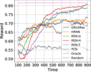
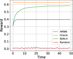
Results. Fig. 1 shows the rewards over time for different methods. Results are averaged over runs and we plot the rolling average with a window size of to prevent clutter. As expected, conventional RNN-based recommenders saturate at around the -th time step, while all REN variants successfully achieve nearly optimal rewards in the end. One interesting observation is that REN variants obtain rewards lower than the “Random" baseline at the beginning, meaning that they are sacrificing immediate rewards to perform exploration in exchange for long-term rewards.
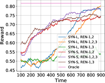
Ablation Study. Fig. 2 shows the rewards over time for REN-G (i.e., REN-1,2,3), REN-1,2, and REN-1,3 in SYN-S and SYN-L. We observe that REN-1,2, with only the relevance (first) and diversity (second) terms of Eqn. 5, saturates prematurely in SYN-S. On the other hand, the reward of REN-1,3, with only the relevance (first) and uncertainty (third) term, barely increases over time in SYN-L. In contrast, the full REN-G works in both SYN-S and SYN-L. This is because without the uncertainty term, REN-1,2 fails to effectively choose items with uncertain embeddings to explore. REN-1,3 ignores the diversity in the latent space and tends to explore items that have rarely been recommended; such exploration directly in the item space only works when the item number is small, e.g., in SYN-S.
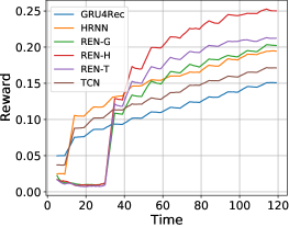

Hyperparameters. For the base models GRU4Rec, TCN, and HRNN, we use identical network architectures and hyperparemeters whenever possible following (Hidasi et al. 2016; Bai, Kolter, and Koltun 2018; Ma et al. 2020). Each RNN consists of an encoding layer, a core RNN layer, and a decoding layer. We set the number of hidden neurons to for all models including REN variants. Fig. 1 in the Supplement shows the REN-G’s performance for different (note that we fix ) in SYN-S, SYN-M, and SYN-L. We can observe stable REN performance across a wide range of . As expected, REN-G’s performance is closer to GRU4Rec when is small.
Real-World Experiments
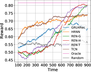
MovieLens-1M. We use MovieLens-1M (Harper and Konstan 2016) containing movies and users with an experiment setting similar to Sec. Simulated Experiments. Each user has interactions, and we follow the joint learning and exploration procedure described in Sec. Experiment Setup and Compared Methods to evaluate all methods (more details in the Supplement). All models recommend items at each round for a chosen user, and the precision@ is used as the reward. Fig. 3(left) shows the rewards over time averaged over all users. As expected, REN variants with different base models are able to achieve higher long-term rewards compared to their non-REN counterparts.
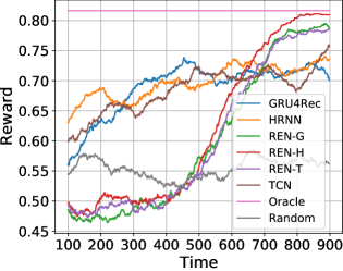
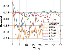
Trivago. We also evaluate the proposed methods on Trivago444More details are available at https://recsys.trivago.cloud/challenge/dataset/., a hotel recommendation dataset with users, items, and interactions. We use a subset with users, items, and interactions and slice the data into one-hour time intervals for the online experiment (see the Supplement for details on data pre-processing). Different from MovieLens-1M, Triavago has impression data available: at each time step, besides which item is clicked by the user, we also know which items are being shown to the user. Such information makes the online evaluation more realistic, as we now know the ground-truth feedback if an arbitrary subset of the items are presented to the user. At each time step of the online experiments, all methods will choose items from the items to recommend the current user and collect the feedback for these items as data for finetuning. We pretrain the model using all items from the first hours before starting the online evaluation. Fig. 3(middle) shows the mean reciprocal rank (MRR), the official metric used in the RecSys Challenge, for different methods. As expected, the baseline RNN (e.g., GRU4Rec) suffers from a drastic drop in rewards because agents are allowed to recommend only items, and they choose to focus only on relevance. This will inevitably ignores valuable items and harms the accuracy. In contrast, REN variants (e.g., REN-G) can effectively balance relevance and exploration for these recommended items at each time step, achieving higher long-term rewards. Interestingly, we also observe that REN variants have better stability in performance compared to RNN baselines.
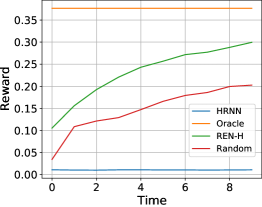
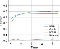
Netflix. Finally, we also use Netflix555https://www.kaggle.com/netflix-inc/netflix-prize-data to evaluate how REN performs in the slate recommendation setting and without finetuning in each time step, i.e., skipping Step (3) in Sec. Experiment Setup and Compared Methods. We pretrain REN on data from half the users and evaluate on the other half. At each time step, REN generates 100 mutually diversified items for one slate following Eqn. 5, with updated after every item generation. Fig. 3(right) shows the recall@100 as the reward for different methods, demonstrating REN’s promising exploration ability when no finetuning is allowed (more results in the Supplement). Fig. 4(left) shows similar trends with recall@100 as the reward on the same holdout item set. This shows that the collected set contributes to building better user embedding models. Fig. 4(middle) shows that the additional exploration power comes without significant harms to the user’s immediate rewards on the exploration set, where the recommendations are served. In fact, we used a relatively large exploration coefficient, , which starts to affect recommendation results on the sixth position. By additional hyperparameter tuning, we realized that to achieve better rewards on the exploration set, we may choose smaller and . Fig. 4(right) shows significantly higher recalls close to the oracle performance, where all of the users’ histories are known and used as inputs to predict the top-100 personalized recommendations.666The gap between oracle and 100% recall lies in the model approximation errors. Note that, for fair presentation of the tuned results, we switched the exploration set and the holdout set and used a different test user group, consisting of 1543 users. We believe that the tuned results are generalizable with new users and items, but we also realize that the Netflix dataset still has a significant popularity bias and therefore we recommend using larger exploration coefficients with real online systems. The inference cost is 175 milliseconds to pick top-100 items from 8000 evaluation items. It includes 100 sequential linear function solutions with 50 embedding dimensions, which is further improvable by selecting multiple items at a time in slate generation.
Conclusion
We propose the REN framework to balance relevance and exploration during recommendation. Our theoretical analysis and empirical results demonstrate the importance of considering uncertainty in the learned representations for effective exploration and improvement on long-term rewards. We provide an upper confidence bound on the estimated rewards along with its corresponding regret bound and show that REN can achieve the same rate-optimal sublinear regret even in the presence of uncertain representations. Future work could investigate the possibility of learned uncertainty in representations, extension to Thompson sampling, nonlinearity of the reward w.r.t. , and applications beyond recommender systems, e.g., robotics and conversational agents.
Acknowledgement
The authors thank Tim Januschowski, Alex Smola, the AWS AI’s Personalize Team and ML Forecast Team, as well as the reviewers/SPC/AC for the constructive comments to improve the paper. We are also grateful for the RecoBandits package provided by Bharathan Blaji, Saurabh Gupta, and Jing Wang to facilitate the simulated environments. HW is partially supported by NSF Grant IIS-2127918.
References
- Agarwal et al. (2014) Agarwal, A.; Hsu, D. J.; Kale, S.; Langford, J.; Li, L.; and Schapire, R. E. 2014. Taming the Monster: A Fast and Simple Algorithm for Contextual Bandits. In ICML, 1638–1646.
- Antikacioglu and Ravi (2017) Antikacioglu, A.; and Ravi, R. 2017. Post processing recommender systems for diversity. In KDD, 707–716.
- Auer (2002) Auer, P. 2002. Using Confidence Bounds for Exploitation-Exploration Trade-offs. JMLR, 3: 397–422.
- Bai, Kolter, and Koltun (2018) Bai, S.; Kolter, J. Z.; and Koltun, V. 2018. An Empirical Evaluation of Generic Convolutional and Recurrent Networks for Sequence Modeling. CoRR, abs/1803.01271.
- Belletti, Chen, and Chi (2019) Belletti, F.; Chen, M.; and Chi, E. H. 2019. Quantifying Long Range Dependence in Language and User Behavior to improve RNNs. In KDD, 1317–1327.
- Bello et al. (2018) Bello, I.; Kulkarni, S.; Jain, S.; Boutilier, C.; Chi, E.; Eban, E.; Luo, X.; Mackey, A.; and Meshi, O. 2018. Seq2slate: Re-ranking and slate optimization with rnns. arXiv preprint arXiv:1810.02019.
- Chen et al. (2019) Chen, M.; Beutel, A.; Covington, P.; Jain, S.; Belletti, F.; and Chi, E. H. 2019. Top-k off-policy correction for a REINFORCE recommender system. In WSDM, 456–464.
- Cho et al. (2014) Cho, K.; van Merrienboer, B.; Gulcehre, C.; Bahdanau, D.; Bougares, F.; Schwenk, H.; and Bengio, Y. 2014. Learning Phrase Representations using RNN Encoder-Decoder for Statistical Machine Translation. In EMNLP, 1724–1734.
- Chu et al. (2011) Chu, W.; Li, L.; Reyzin, L.; and Schapire, R. 2011. Contextual bandits with linear payoff functions. In AISTATS, 208–214.
- Ding et al. (2021) Ding, H.; Ma, Y.; Deoras, A.; Wang, Y.; and Wang, H. 2021. Zero-Shot Recommender Systems. arXiv preprint arXiv:2105.08318.
- Fang et al. (2019) Fang, H.; Zhang, D.; Shu, Y.; and Guo, G. 2019. Deep Learning for Sequential Recommendation: Algorithms, Influential Factors, and Evaluations. arXiv preprint arXiv:1905.01997.
- Foster et al. (2018) Foster, D. J.; Agarwal, A.; Dudík, M.; Luo, H.; and Schapire, R. E. 2018. Practical Contextual Bandits with Regression Oracles. In ICML, 1534–1543.
- Friedland and Gaubert (2013) Friedland, S.; and Gaubert, S. 2013. Submodular spectral functions of principal submatrices of a hermitian matrix, extensions and applications. Linear Algebra and its Applications, 438(10): 3872–3884.
- Gupta et al. (2021) Gupta, S.; Wang, H.; Lipton, Z.; and Wang, Y. 2021. Correcting exposure bias for link recommendation. In ICML.
- Harper and Konstan (2016) Harper, F. M.; and Konstan, J. A. 2016. The movielens datasets: History and context. ACM Transactions on Interactive Intelligent Systems (TiiS), 5(4): 19.
- Hidasi et al. (2016) Hidasi, B.; Karatzoglou, A.; Baltrunas, L.; and Tikk, D. 2016. Session-based Recommendations with Recurrent Neural Networks. In ICLR.
- Hiranandani et al. (2019) Hiranandani, G.; Singh, H.; Gupta, P.; Burhanuddin, I. A.; Wen, Z.; and Kveton, B. 2019. Cascading Linear Submodular Bandits: Accounting for Position Bias and Diversity in Online Learning to Rank. In UAI, 248.
- Jun et al. (2019) Jun, K.-S.; Willett, R.; Wright, S.; and Nowak, R. 2019. Bilinear Bandits with Low-rank Structure. In Chaudhuri, K.; and Salakhutdinov, R., eds., Proceedings of the 36th International Conference on Machine Learning, volume 97 of Proceedings of Machine Learning Research, 3163–3172. PMLR.
- Kingma and Welling (2014) Kingma, D. P.; and Welling, M. 2014. Auto-Encoding Variational Bayes. In ICLR.
- Korda, Szorenyi, and Li (2016) Korda, N.; Szorenyi, B.; and Li, S. 2016. Distributed clustering of linear bandits in peer to peer networks. In ICML, 1301–1309.
- Kveton et al. (2017) Kveton, B.; Szepesvári, C.; Rao, A.; Wen, Z.; Abbasi-Yadkori, Y.; and Muthukrishnan, S. 2017. Stochastic Low-Rank Bandits. CoRR, abs/1712.04644.
- Li et al. (2017) Li, J.; Ren, P.; Chen, Z.; Ren, Z.; Lian, T.; and Ma, J. 2017. Neural attentive session-based recommendation. In CIKM, 1419–1428.
- Li et al. (2010) Li, L.; Chu, W.; Langford, J.; and Schapire, R. E. 2010. A contextual-bandit approach to personalized news article recommendation. In WWW, 661–670.
- Li, Karatzoglou, and Gentile (2016) Li, S.; Karatzoglou, A.; and Gentile, C. 2016. Collaborative Filtering Bandits. In SIGIR, 539–548.
- Li and She (2017) Li, X.; and She, J. 2017. Collaborative Variational Autoencoder for Recommender Systems. In KDD, 305–314.
- Liu et al. (2018) Liu, Q.; Zeng, Y.; Mokhosi, R.; and Zhang, H. 2018. STAMP: short-term attention/memory priority model for session-based recommendation. In KDD, 1831–1839.
- Ma et al. (2020) Ma, Y.; Narayanaswamy, M. B.; Lin, H.; and Ding, H. 2020. Temporal-Contextual Recommendation in Real-Time. In KDD.
- Mahadik et al. (2020) Mahadik, K.; Wu, Q.; Li, S.; and Sabne, A. 2020. Fast distributed bandits for online recommendation systems. In SC, 1–13.
- Mi et al. (2019) Mi, L.; Wang, H.; Tian, Y.; and Shavit, N. 2019. Training-Free Uncertainty Estimation for Neural Networks. arXiv e-prints, arXiv–1910.
- Nguyen et al. (2014) Nguyen, T. T.; Hui, P.-M.; Harper, F. M.; Terveen, L.; and Konstan, J. A. 2014. Exploring the filter bubble: the effect of using recommender systems on content diversity. In WWW, 677–686.
- Osband, Van Roy, and Wen (2016) Osband, I.; Van Roy, B.; and Wen, Z. 2016. Generalization and exploration via randomized value functions. In ICML, 2377–2386.
- Quadrana et al. (2017) Quadrana, M.; Karatzoglou, A.; Hidasi, B.; and Cremonesi, P. 2017. Personalizing Session-based Recommendations with Hierarchical Recurrent Neural Networks. In RecSys, 130–137.
- Salakhutdinov, Mnih, and Hinton (2007) Salakhutdinov, R.; Mnih, A.; and Hinton, G. E. 2007. Restricted Boltzmann machines for collaborative filtering. In ICML, volume 227, 791–798.
- Shi et al. (2019) Shi, J.-C.; Yu, Y.; Da, Q.; Chen, S.-Y.; and Zeng, A.-X. 2019. Virtual-taobao: Virtualizing real-world online retail environment for reinforcement learning. In AAAI, volume 33, 4902–4909.
- Tang et al. (2019) Tang, J.; Belletti, F.; Jain, S.; Chen, M.; Beutel, A.; Xu, C.; and H. Chi, E. 2019. Towards neural mixture recommender for long range dependent user sequences. In WWW, 1782–1793.
- Tschiatschek, Djolonga, and Krause (2016) Tschiatschek, S.; Djolonga, J.; and Krause, A. 2016. Learning Probabilistic Submodular Diversity Models Via Noise Contrastive Estimation. In AISTATS, 770–779.
- van den Oord, Dieleman, and Schrauwen (2013) van den Oord, A.; Dieleman, S.; and Schrauwen, B. 2013. Deep content-based music recommendation. In NIPS, 2643–2651.
- Vanchinathan et al. (2014) Vanchinathan, H. P.; Nikolic, I.; Bona, F. D.; and Krause, A. 2014. Explore-exploit in top-N recommender systems via Gaussian processes. In RecSys, 225–232.
- Wang (2017) Wang, H. 2017. Bayesian Deep Learning for Integrated Intelligence: Bridging the Gap between Perception and Inference. Ph.D. thesis, Hong Kong University of Science and Technology.
- Wang, Shi, and Yeung (2015) Wang, H.; Shi, X.; and Yeung, D. 2015. Relational stacked denoising autoencoder for tag recommendation. In AAAI, 3052–3058.
- Wang, Shi, and Yeung (2016) Wang, H.; Shi, X.; and Yeung, D.-Y. 2016. Collaborative recurrent autoencoder: Recommend while learning to fill in the blanks. In NIPS, 415–423.
- Wang, Wang, and Yeung (2015) Wang, H.; Wang, N.; and Yeung, D. 2015. Collaborative deep learning for recommender systems. In KDD, 1235–1244.
- Wang, Xingjian, and Yeung (2016) Wang, H.; Xingjian, S.; and Yeung, D.-Y. 2016. Natural-parameter networks: A class of probabilistic neural networks. In NIPS, 118–126.
- Wang and Yeung (2016) Wang, H.; and Yeung, D.-Y. 2016. Towards Bayesian deep learning: A framework and some existing methods. TDKE, 28(12): 3395–3408.
- Wang and Yeung (2020) Wang, H.; and Yeung, D.-Y. 2020. A Survey on Bayesian Deep Learning. ACM Computing Surveys (CSUR), 53(5): 1–37.
- Wilhelm et al. (2018) Wilhelm, M.; Ramanathan, A.; Bonomo, A.; Jain, S.; Chi, E. H.; and Gillenwater, J. 2018. Practical diversified recommendations on youtube with determinantal point processes. In CIKM, 2165–2173.
- Wu et al. (2019) Wu, S.; Tang, Y.; Zhu, Y.; Wang, L.; Xie, X.; and Tan, T. 2019. Session-based recommendation with graph neural networks. In AAAI, volume 33, 346–353.
- Yue and Guestrin (2011) Yue, Y.; and Guestrin, C. 2011. Linear Submodular Bandits and their Application to Diversified Retrieval. In NIPS, 2483–2491.
- Zhou, Li, and Gu (2019) Zhou, D.; Li, L.; and Gu, Q. 2019. Neural Contextual Bandits with Upper Confidence Bound-Based Exploration. arXiv preprint arXiv:1911.04462.
Appendix A Proofs in the Main Paper
In this section, we provide the detailed proofs for the lemmas and main theorem in the paper.
Assumption 2.
Assume there exists an optimal , with and such that . Further assume that there is an effective distribution such that where . Thus, the true underlying context is unavailable, but we are aided with the knowledge that it is generated with a multivariate normal whose parameters are known.
Upper Confidence Bound for Uncertain Embeddings
For simplicity we follow the notation from (Chu et al. 2011) and denote the item embedding (context) as , where indexes the rounds and indexes the items. We define:
where is the collected user feedback. Lemma 6 below shows that with and , the main equation in the paper is the upper confidence bound with high probability, meaning that it upper bounds the true reward with high probability, which makes it a reasonable score for recommendations.
Lemma 6 (Confidence Bound).
With probability at least , we have for all that
where is the norm.
Proof.
Using the notation defined above, we have
| (8) | |||
| (9) |
To see Eqn. 8 is true, note that . To see Eqn. 9 is true, note that since , we have . Similarly for the last term in Eqn. 9, observe that
| (10) |
For the first term in Eqn. 9, since , and is a random variable bounded by , by Azuma-Hoeffding inequality, we have
| (11) | ||||
| (12) |
where Eqn. 11 is due to
For the second term of Eqn. 9, , since , we can guarantee that with probability at most ,
| (13) |
where is the operator norm of the matrix corresponding to the vector norm.
Regret Bound
Lemma 6 above provides a reasonable estimate of the reward’s upper bound at time . Based on this estimate, one natural next step is to analyze the regret after all rounds. Formally, we define the regret of the algorithm after rounds as
| (14) |
where is the optimal item (action) at round that maximizes , and is the action chose by the algorithm at round . In a similar fashion as in (Chu et al. 2011), SupREN calls BaseREN as a sub-routine. In this subsection, we derive the regret bound for SupREN with uncertain item embeddings.
Lemma 7 (Azuma–Hoeffding Inequality).
Let be random variables with for some . Then we have
Lemma 8.
With probability , for any and any :
-
1.
for any ,
-
2.
, and
-
3.
for any .
Proof.
Lemma 9.
In BaseREN, we have
Proof.
Lemma 10.
Assuming and for any and , then for any ,
Proof.
Since the function is convex when , we have
∎
Lemma 11.
For all ,
Proof.
Theorem 2.
If SupREN is run with , with probability at least , the regret of the algorithm is
| (19) |
Proof.
The proof is an extension of Theorem 6 in (Auer 2002) to handle the uncertainty in item embeddings. We denote as the set of trials for which an alternative is chosen in Line 4 of Algorithm 4. Note that ; therefore . We have
| (20) | ||||
| (21) | ||||
| (22) |
with probability . Eqn. 20 is by Lemma 8, and Eqn. 21 is by Lemma 11. By the Azuma-–Hoeffding inequality (Lemma 7) with and , we have
| (23) |
with probability at least . To see this, note that and that
Replacing by and by in Eqn. 23 along with simplification gives us
with probability . Therefore we have
with probability . ∎
Theorem 2 shows that even with the uncertainty in the item embeddings, our proposed REN can achieve the same rate-optimal sublinear regret bound as in (Chu et al. 2011).
Appendix B More Details on Datasets
MovieLens-1M
We use MovieLens-1M (Harper and Konstan 2016) containing movies and users. Each user has interactions, and we follow the joint learning and exploration procedure described in the main paper to evaluate all methods.
Trivago
Trivago is a hotel recommendation dataset with users, items, and interactions. We use a subset with users, items, and interactions and slice the data into one-hour time intervals for the online experiment. Different from MovieLens-1M, Triavago has impression data available. Specifically, at each time step, besides which item is clicked by the user, we also know which items are being shown to the user. Essentially the RecSys Challenge is a reranking problem with candidate sets of size .
Netflix
Our main conclusion with Netflix experiments is that REN-inference-only procedure collects more diverse data points about a user, which allows us to build a more generalizable user model, which leads to better long-term rewards. The main paper demonstrates better generalizability by comparing precision@100 reward on a holdout item set, where the items are inaccessible to the user - i.e., we never collect feedback on these holdout items in our simulations. Instead, recommendations are made by comparing the users’ learned embeddings and the pretrained embeddings of the holdout items.
Appendix C Hyperparameters and Neural Network Architectures
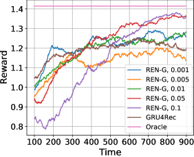
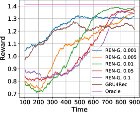
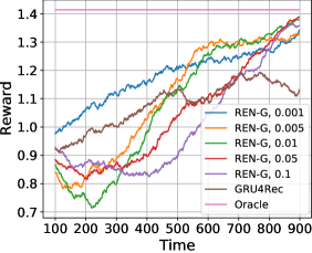
For the base models GRU4Rec, TCN, and HRNN, we use identical network architectures and hyperparemeters whenever possible following (Hidasi et al. 2016; Bai, Kolter, and Koltun 2018; Ma et al. 2020). Each RNN consists of an encoding layer, a core RNN layer, and a decoding layer. We set the number of hidden neurons to for all models including REN variants. Fig. 5 shows the REN-G’s performance for different (note that we fix ) in SYN-S, SYN-M, and SYN-L. We can observe stable REN performance across a wide range of . As expected, REN-G’s performance is closer to GRU4Rec when is small.