AGN impact on the molecular gas in galactic centers as probed by CO lines

Abstract

We present a detailed analysis of the X-ray, infrared, and carbon monoxide (CO) emission for a sample of 35 local ($z\leq 0.15$), active ($L_{\text{X}}\geq 10^{42}$ erg s^-1) galaxies. Our goal is to infer the contribution of far-ultraviolet (FUV) radiation from star formation (SF), and X-ray radiation from the active galactic nuclei (AGN), respectively producing photodissociation regions (PDRs) and X-ray dominated regions (XDRs), to the molecular gas heating. To this aim, we exploit the CO spectral line energy distribution (CO SLED) as traced by Herschel, complemented with data from single-dish telescopes for the low-$J$ lines, and high-resolution ALMA images of the mid-$J$ CO emitting region. By comparing our results to the Schmidt-Kennicutt relation, we find no evidence for AGN influence on the cold and low-density gas on kpc-scales. On nuclear ($r=250$ pc) scales, we find weak correlations between the CO line ratios and either the FUV or X-ray fluxes: this may indicate that neither SF nor AGN radiation dominates the gas excitation, at least at $r=250$ pc. From a comparison of the CO line ratios with PDR and XDR models, we find that PDRs can reproduce observations only in presence of extremely high gas densities ($n>10^{5}$ cm^-3). In the XDR case, instead, the models suggest moderate densities ($n\approx 10^{2-4}$ cm^-3). We conclude that a mix of the two mechanisms (PDR for the mid-$J$, XDR or possibly shocks for the high-$J$) is necessary to explain the observed CO excitation in active galaxies.

1 Introduction

The molecular gas phase of the interstellar medium (ISM) is the fuel for star formation (SF), thus it plays a central role in galaxy evolution (McKee & Ostriker, 2007; Carilli & Walter, 2013; Tacconi et al., 2020). At the same time, the molecular gas properties (e.g. temperature, density, turbulence, chemical composition) are affected by feedback processes induced by SF and by the accretion onto the central black hole in sources hosting an active galactic nucleus (AGN) (Aalto et al., 1995; Omont, 2007; Imanishi et al., 2011, 2016). A key question is whether, and on which spatial scales, the effect of AGN radiation on the molecular gas can produce observable effects that can be retrieved from the molecular line emission.

Molecular hydrogen (H₂), dominating the mass of molecular ISM, does not have a dipole moment, and the quadrupole transitions require high temperatures ($T=500-2000\rm\,K$), mainly present in shock-heated gas (Flower & Pineau Des Forêts, 2010). For this reason, the most used molecular gas tracer is the carbon monoxide (CO) which has instead bright dipole emission and is the second most abundant molecule in the Universe (Bolatto et al., 2013).

Moreover, the CO Spectral Line Energy Distribution (CO SLED), i.e. the luminosity of CO rotational lines as a function of the rotational quantum number $J$, is a very powerful diagnostic for the physical conditions of molecular ISM (Narayanan & Krumholz, 2014; Rosenberg et al., 2015). The CO SLED can be broken down into three different parts (e.g. Vallini et al., 2019; Decarli et al., 2020). The low-$J$ lines ($J_{\text{upp}}\leq 3$) trace the cold ($T\approx 20-50$ K), low-density ($n\lesssim 10^{3}$ cm^-3) gas; this is where the majority of the mass resides, so these lines are good tracers of the total molecular gas mass in galaxies (Bolatto et al., 2013). Both the mid-$J$ ($4\leq J_{\text{upp}}\leq 7$) and the high-$J$ ($J_{\text{upp}}\geq 8$) lines originate from increasingly denser ($n\approx 10^{4}-10^{6}$ cm^-3) and warmer ($T\approx 100-500$ K) molecular gas (Greve et al., 2014). For this reason, the excitation of the CO ladder, especially in the mid/high-$J$ part, can be exploited to disentangle different heating sources such as radiation from SF, AGN accretion, and mechanical heating from shocks (e.g. van der Werf et al., 2010; Mingozzi et al., 2018).

Stellar radiation affects the molecular gas mainly in the far-ultraviolet (FUV, $6<h\nu<13.6\rm\,eV$) band, where photons can dissociate H₂ molecules without ionizing H atoms (for which photons with $h\nu\geq 13.6$ eV are needed). The FUV photon penetration creates a transition layer, called photodissociation region (PDR), linking the outer HII region and the fully molecular layers of Giant Molecular Clouds (GMCs). FUV-induced photoelectric effect on dust grains is the major heating mechanism in PDRs (Hollenbach & Tielens, 1997, 1999), which then cool down through metal fine structure line emission (e.g. [CII] $158\,\rm\mu m$, [OI] $63\,\rm\mu m$) and molecular rotational lines, among which CO transitions. The FUV flux is usually parametrized in terms of the Habing field ($G_{0}=1.6\times 10^{-3}$ erg s^-1 cm^-2, Habing 1968).

X-ray photons from the AGN penetrate deeper than FUV photons into the molecular clouds and create the so-called X-ray Dominated Regions (XDR; Maloney et al., 1996). There, the heating and chemical composition of the gas are peculiarly influenced by the $\sim$1–100 keV X-ray radiation (Maloney et al., 1996; Meijerink & Spaans, 2005; Meijerink et al., 2007), keeping the molecular gas warmer at larger (column) densities, following the release of fast photoelectrons (Morrison & McCammon, 1983; Wilms et al., 2000).

PDR and XDR models are radiative transfer calculations (Hollenbach & Tielens, 1999; Meijerink et al., 2007; Ferland et al., 2017) that take the impinging radiation (FUV and X-ray photons, respectively), the gas density, column density, and metallicity as input, and return the expected line emission. While the low/mid-$J$ CO emission is usually consistent with the presence of a PDR component produced by SF (Pereira-Santaella et al., 2013; Kamenetzky et al., 2014; Talia et al., 2018), in active galaxies with peculiarly excited high-$J$ CO lines (van der Werf et al., 2010; Schleicher et al., 2010; Gallerani et al., 2014; Pozzi et al., 2017; Vallini et al., 2019; Pensabene et al., 2021) an XDR, associated with the AGN activity, is often necessary to reproduce the CO SLEDs.

The purpose of this work is to investigate the possible relation between the AGN activity and the conditions of molecular gas in a sample of local active galaxies with well-sampled CO SLED. We will assess whether, and to what extent, the excitation of the CO ladder shows correlations with X-ray and FUV tracers and whether the CO SLED can be used to infer the effect of SF versus AGN heating on the whole host galaxy and within the nuclear region.

The paper is structured as follows: in Section 2 we introduce the sample and the selection criteria. In Section 3 we describe the data collection from the sub-mm up to the X-ray band. In Section 4 we derive the CO emission on a galactic scale, and we study the Schmidt–Kennicutt relation. In Section 5 we derive the physical parameters for the PDR and XDR analysis and we discuss the results we find. We assume a $\Lambda$CDM cosmology with $H_{0}=70$ km s^-1 Mpc^-1, $\Omega_{m}=0.3$ and $\Omega_{\Lambda}=0.7$.

2 Sample selection

Table 1: Properties of the sample of 35 AGN.

	RA	Dec	$D_{\rm L}$	D25	Class	log$L_{\rm X}$	log$N_{\rm H}$	logL${}_{\text{IR}}$	logM${}_{\text{mol}}$	SFR	Sample
Name	(deg)	(deg)	(Mpc)	(′′)		(erg s-1)	(cm-2)	(L⊙)	(M⊙)	(M⊙ yr-1)
NGC 0034	2.78	-12.11	85	69	S2	42.11	23.72	11.44	9.97	31	klr-sn
UGC 00545	13.40	12.69	264	29	Q	43.60	–	11.95${}^{\text{d}}$	10.17	34	k-n
NGC 1068	40.67	-0.01	16	370	S1h	42.38	24.70	11.27	10.14	17	klmr-cbn
3C 84	49.95	41.51	76	128	S1.5	43.98	21.68	11.20	9.63	9.0	kl-b
NGC 1365	53.40	-36.14	23	721	S1.8	42.32	22.21	11.00	10.10	17	kr-bn
IRAS F05189-2524	80.26	-25.36	188	30	S1h	43.20	22.86	12.11	10.04	109	klpr-sbn
IRAS 07598+6508	121.14	65.00	704	39${}^{\text{c}}$	S1	42.10	–	12.46${}^{\text{e}}$	10.54	–	kp-n
UGC 05101	143.97	61.35	174	72	S1	43.08	24.08	11.95	10.21	105	klp-xbn
NGC 3227	155.88	19.87	17	239	S	42.10	20.95	10.13	9.02	0.56	k-bn
NGC 4151	182.64	39.41	14	173	S	42.31	22.71	10.20	7.42	0.25	k-bn
NGC 4388	186.45	12.66	36	322	S1h	42.60	23.50	10.00	9.40	3.7	k-sbn
TOL 1238-364	190.22	-36.76	47	76	S1h	43.40	24.95	10.62	8.94	4.1	k-s
Mrk 0231	194.06	56.87	186	85	S1	42.50	22.85	12.51	10.39	278	klpmr-n
MCG -03-34-064	200.60	-16.73	72	81	S1h	43.18	23.80	11.24	–	5.7	kl-sbn
NGC 5128	201.37	-43.02	8	1542	S2${}^{\text{i}}$	42.39	23.02	10.11	10.17	6.7	k-b
NGC 5135	201.43	-29.83	59	144	S2	41.97	24.47	11.17	10.17	17	rlk-s
Mrk 0463	209.01	18.37	224	64	S1h	43.28	23.83	11.77${}^{\text{e}}$	9.92	–	kp-sbn
IC 4518a	224.42	-43.13	71	55	S2	42.64	23.36	11.13	–	5.6	kl-b
VV 705${}^{\text{a}}$	229.53	42.75	177	39	S2${}^{\text{i}}$	42.30	23.93	11.89	10.37	72	kl-n
PKS 1549-79	239.25	-79.24	725	–	S1i	44.71	20.00	12.36${}^{\text{d}}$	10.01${}^{\text{h}}$	–	k-b
PG 1613+658	243.49	65.72	605	27	Q	44.19	20.00	12.00	10.24	44	k-b
NGC 6240	253.25	2.40	107	131	S3	43.58	24.20	11.85	10.58	70	klpmr-cbn
IRAS 19254-7245${}^{\text{b}}$	292.84	-72.66	277	38	S2${}^{\text{i}}$	42.80	23.58	12.06${}^{\text{e}}$	10.34	104	kp-n
3C 405	299.87	40.73	250	33	S1.9	44.37	23.38	<11.75${}^{\text{g}}$	<8.88	35	k-b
MCG +04-48-002	307.15	25.73	60	60	S2${}^{\text{i}}$	43.13	23.86	11.06	9.64	10	kl-b
IC 5063	313.01	-57.07	49	161	S1h	42.87	23.42	10.85	9.36	2.6	k-sb
ESO 286-IG019	314.61	-42.65	190	41	H2	42.30	23.69	12.00	10.25	105	klp-n
3C 433	320.94	25.07	468	19	S2	44.16	23.01	<11.66${}^{\text{g}}$	<9.71	10	k-b
NGC 7130	327.08	-34.95	70	93	S1.9	42.30	24.10	11.35	10.10	22	kl-scb
NGC 7172	330.51	-31.87	37	151	S2	42.76	22.91	10.45	9.58	2.5	k-bn
NGC 7465	345.50	15.97	28	64	S3	41.97	21.46	10.10	8.88	0.76	k-b
NGC 7469	345.82	8.87	71	83	S	43.19	20.53	11.59	10.09	35	klr-bn
ESO 148-IG002	348.95	-59.05	198	56	H2	43.20	–	12.00	10.05	108	klp-n
NGC 7582	349.60	-42.37	23	415	S1i	42.53	24.20	10.87	9.64	7.1	k-cbn
NGC 7674	351.99	8.78	127	67	S1h	43.60	–	11.50	10.46	15	kl-n

• Notes. RA, Dec from NED. $D_{\rm L}$ is the luminosity distance, calculated from the redshift (taken from NED) according to the adopted cosmology. D₂₅ is the optical diameter, measured at the isophotal level 25 mag arcsec^-2 in the B-band, taken from HyperLEDA. Class is the AGN classification from HyperLEDA: Q = quasar, S1 = broad-line Seyfert 1, S1i = S1 with a broad Paschen H$\beta$ line, S1h = S2 which show S1 like spectra in polarized light, S2 = Seyfert 2, S1.5 = Seyfert 1.5, S1.8 = Seyfert 1.8, S1.9 = Seyfert 1.9, S = AGN objects without classification, S3 = LINERs, H2 = extragalactic HII regions. $L_{\rm X}$ is the 2–10 keV intrinsic (i.e. corrected for source absorption) luminosity, taken from the works indicated in the Sample column (see Section 3.1 for details). L${}_{\text{IR}}$ is the 8–1000 $\mu$m luminosity, from Sanders et al. (2003) unless otherwise specified. M${}_{\text{mol}}$ is the total molecular mass, calculated as described in Section 3.5. SFR is the star formation rate, calculated as described in Section 5.1. Sample lists the references for the CO Herschel fluxes ($r$ for Rosenberg et al. (2015), $m$ for Mashian et al. (2015), $p$ for Pearson et al. (2016), $k$ for Kamenetzky et al. (2016), $l$ for Lu et al. (2017)) and for the X-ray data ($n$ for Brightman & Nandra (2011), $b$ for Ricci et al. (2017a), $c$ for Marchesi et al. (2019), $x$ for La Caria et al. (2019), $s$ for Salvestrini et al. (2022, in prep.)).

  Additional notes. (a) RA, Dec from Kojoian et al. (1981). (b) RA, Dec from Westmoquette et al. (2012). (c) D₂₅ from NED. (d) L${}_{\text{IR}}$ from Moshir et al. (1990). (e) L${}_{\text{IR}}$ from Pearson et al. (2016). (f) L${}_{\text{IR}}$ from the IRAS PSC (1988). (g) Upper limit for L${}_{\text{IR}}$ from Golombek et al. (1988). (h) M${}_{\text{H}_{2}}$ from Oosterloo et al. (2019). (i) Class from NED.

To investigate the impact of AGN activity onto the molecular gas, we select a sample of local galaxies adopting the following criteria: (i) a properly sampled CO SLED in the mid/high-$J$ regimes from Herschel observations; (ii) an intrinsic $2-10$ keV luminosity L${}_{X}\geq 10^{42}$ erg s^-1. Moreover, we collect low/mid-$J$ CO data by considering both sub-mm/mm single-dish observations, and interferometric ALMA data, which ensure a high spatial resolution.

Selecting sources with intrinsic L${}_{\text{X}}\geq 10^{42}$ erg s^-1 is the standard criterion for identifying AGN, since stellar processes alone (e.g. X-ray binaries, hot ionized ISM) rarely reach this X-ray luminosity (Hickox & Alexander, 2018). We look for AGN with a well-sampled CO SLED, to be able to study the high-$J$ lines ($J_{\text{upp}}\geq 8$), where we expect to find the imprint of the AGN influence on the molecular gas.

The adopted criteria lead to a sample of 35 active galaxies (see Table 1), with redshifts in the range $0.0015<z<0.15$ (median $z=0.02$), corresponding to luminosity distances ($D_{\rm L}$) in the range $4-720$ Mpc.

Considering the classification from the optical spectra, $92\%$ of our AGN are classified as Seyfert galaxies and two (VV 705 and ESO186–IG019) as low-ionisation nuclear emission line regions (LINERs). One of our sources (PKS 1549–79) is a quasar (see Netzer 2015 for a review on AGN classification), while PKS 1549-79, 3C84 (Perseus A, NGC 1275), 3C405 (Cygnus A), and 3C433 are also known as radio sources.

The $8-1000$ $\mu$m infrared luminosities $L_{\text{IR}}$ (from Sanders et al., 2003) cover the range $10^{10}L_{\odot}<L_{\text{IR}}<10^{12.5}L_{\odot}$. The bulk ($43\%$) of our sample is made of luminous infrared galaxies (LIRGs, $10^{11}\leq L_{\text{IR}}/L_{\odot}<10^{12}$), while ultra-luminous infrared galaxies (ULIRGs, $L_{\text{IR}}\geq 10^{12}L_{\odot}$) account for $27\%$ of the sample; the remaining $30\%$ have $10^{10}<L_{\text{IR}}<10^{11}L_{\odot}$. It is thought that the (U)LIRG phenomenon is mainly linked to merger activity (Lonsdale et al., 2006), especially for $L_{\text{IR}}\geq 10^{11.5}$ L_⊙ (Hung et al., 2014; Pérez-Torres et al., 2021), as during mergers the gas can reach very high gas densities, triggering intense SF (Larson & Tinsley, 1978). Mergers and interactions can also trigger AGN activity for the very same reason: the gas has the opportunity to lose its angular momentum and fall from kpc-scale distances to the inner parsecs from the nucleus (Alonso-Herrero et al., 2012; Treister et al., 2012; Ricci et al., 2017b; Ellison et al., 2019). Both SF and AGN phenomena heat the dust, hence boosting the IR luminosity of the host galaxies. Within our sample, at least five galaxies show an evolved merging phase: ESO 148-IG002 (Leslie et al., 2014), IRAS 19254-7245 (Superantennae, Bendo et al., 2009), NGC 6240 (Komossa et al., 2003), Mrk 463 (Bianchi et al., 2008) and VV 705 (Perna et al., 2019). Seven more galaxies have a very close companion: NGC 3227 ($\sim$15 kpc, Mundell et al., 2004), NGC 7465 ($\sim$15 kpc, Merkulova et al., 2012), NGC 7469 ($\sim$20 kpc, Zaragoza-Cardiel et al., 2017), NGC 7674 ($\sim$20 kpc, Larson et al., 2016), MCG+04-48-002 ($\sim$25 kpc, Koss et al., 2016), TOL1238-364 ($\sim$25 kpc, Temporin et al., 2003), and IC4518a ($\sim$1 kpc, Bellocchi et al., 2016). Two additional sources (NGC 34 and ESO 286-IG019) have a disturbed morphology, sign of a past galactic interaction. Moreover, some of the galaxies of this sample (notably NGC 5128, 3C84 and 3C405) are known to be part of groups or clusters, so their morphology is unsettled by probable continuous interactions with nearby satellite galaxies. Same as for the (U)LIRGs, interacting galaxies and systems with disturbed morphologies are typically characterized by higher molecular gas content and star-formation activity than isolated galaxies that may be due to tidal torques able to produce gas infall from the surrounding regions (e.g. Combes et al., 1994; Casasola et al., 2004; Pan et al., 2018; Moreno et al., 2019).

3 Data collection

Table 2: CO SLED transitions in units of $\log(L/L_{\odot})$

.

CO transition	1–0	2–1	3–2	4–3	5–4	6–5	7–6	8–7	9–8	10–9	11–10	12–11	13–12
Name
NGC0034	5.22	5.83	–	<6.26	6.57	6.67	6.72	6.75	6.72	6.57	6.63	6.48	6.37
UGC00545	5.42${}^{\text{a}}$	6.25${}^{\text{a}}$	6.92${}^{\text{a}}$	–	–	<7.08	<7.01	<7.15	7.22	<7.14	<7.18	<7.04	<7.17
NGC1068	5.39${}^{\text{b}}$	5.62${}^{\text{b}}$	6.20${}^{\text{a}}$	6.28	6.27	6.28	6.24	6.24	6.17	6.15	6.12	6.08	5.83
3C84	4.85${}^{\text{c}}$	4.48${}^{\text{d}}$	5.92${}^{\text{e}}$	<6.48	6.39	6.32	6.25	6.33	6.41	6.45	6.32	6.31	6.13
NGC1365	5.35	5.50	5.96	6.53	6.60	6.58	6.54	6.48	6.30	6.14	6.08	5.86	<5.77
IRASF05189-2524	5.28${}^{\text{a}}$	6.02${}^{\text{a}}$	6.49${}^{\text{a}}$	<7.04${}^{\text{a}}$	7.06	7.11	7.14	7.22	7.04	7.23	7.15	7.09	7.06
IRAS07598+6508	5.78${}^{\text{f}}$	6.57${}^{\text{f}}$	–	–	<8.08	<7.70	<7.77	<7.62	–	<8.06	<8.00	<8.05	<8.02
UGC05101	5.38${}^{\text{a}}$	6.37${}^{\text{a}}$	6.78${}^{\text{a}}$	–	7.00	7.10	6.95	7.02	6.89	7.05	6.87	6.36	6.69
NGC3227	4.15${}^{\text{g}}$	4.82${}^{\text{h}}$	5.23${}^{\text{h}}$	5.41	5.48	5.44	5.30	5.34	5.19	5.11	5.24	5.15	<5.25
NGC4151	2.55${}^{\text{i}}$	3.23${}^{\text{j}}$	–	<5.14	–	<4.84	4.66	<5.02	<5.14	5.26	<5.24	<5.18	5.03
NGC4388	4.40${}^{\text{h}}$	5.15${}^{\text{h}}$	5.16${}^{\text{h}}$	6.05	5.91	5.94	5.84	5.83	5.78	5.71	<5.96	<5.93	<5.90
TOL1238-364	4.18${}^{\text{k}}$	5.15${}^{\text{k}}$	–	<5.92${}^{\text{k}}$	5.79	5.49	5.30	5.58	5.90	<5.98	<6.06	<5.90	<6.16
Mrk0231	5.54${}^{\text{a}}$	6.39${}^{\text{a}}$	6.83${}^{\text{a}}$	7.25${}^{\text{a}}$	7.28	7.33	7.41	7.44	7.35	7.45	7.36	7.29	7.23
MCG-03-34-064	–	–	–	<6.22	<6.20	5.97	5.96	<6.25	<6.31	6.38	6.05	6.09	6.14
NGC5128	4.85${}^{\text{l}}$	4.57${}^{\text{m}}$	4.90${}^{\text{m}}$	4.51	4.57	4.48	4.32	4.29	<4.48	<4.27	<4.19	<4.24	<4.62
NGC5135	5.19${}^{\text{a}}$	6.00${}^{\text{a}}$	6.38${}^{\text{a}}$	6.51	6.61	6.61	6.49	6.37	6.31	6.13	6.03	5.95	5.65
Mrk0463	5.12${}^{\text{n}}$	5.08${}^{\text{o}}$	–	–	<7.05	6.81	6.67	6.61	<7.03	6.37	<7.05	<7.08	–
IC4518a	–	–	–	6.66	6.28	6.24	5.99	6.14	<6.29	<6.16	6.25	<6.07	<6.28
VV705	5.61${}^{\text{a}}$	5.78${}^{\text{p}}$	6.59${}^{\text{a}}$	–	7.04	6.83	6.95	6.89	<7.04	6.77	6.79	6.79	6.70
PKS1549-79	–	–	–	–	<8.26	<7.95	<7.71	–	–	<7.92	<7.81	<7.98	<7.99
PG1613+658	5.49${}^{\text{f}}$	–	–	–	<7.99	<8.00	–	<7.59	–	<7.83	–	<7.94	<7.87
NGC6240	5.63${}^{\text{a}}$	6.59${}^{\text{a}}$	7.10${}^{\text{a}}$	7.46	7.59	7.69	7.75	7.78	7.75	7.72	7.65	7.59	7.52
IRAS19254-7245	5.59${}^{\text{n}}$	–	–	–	–	7.01	7.31	7.20	7.32	7.21	7.04	6.85	7.07
3C405	<4.12${}^{\text{c}}$	–	–	–	<7.21	<7.01	<6.85	–	<7.21	–	<7.06	–	<7.13
MCG+04-48-002	4.88${}^{\text{q}}$	–	–	<6.61	6.32	6.11	6.13	6.18	<6.25	<6.33	<6.33	<6.18	<6.34
IC5063	4.51${}^{\text{h}}$	–	–	–	<6.17	<5.88	5.77	<6.00	<6.10	<6.15	–	<6.12	<6.17
ESO286-IG019	5.50${}^{\text{r}}$	–	6.30${}^{\text{s}}$	–	7.22	7.13	7.30	7.36	7.22	7.37	7.33	7.25	7.18
3C433	<4.96${}^{\text{c}}$	–	–	–	<7.76	<7.63	<7.38	<7.40	–	<7.37	<7.54	<7.55	–
NGC7130	5.34${}^{\text{q}}$	5.72${}^{\text{p}}$	–	6.70	6.71	6.66	6.62	6.51	6.58	6.43	6.34	6.18	6.11
NGC7172	4.75${}^{\text{p}}$	5.25${}^{\text{t}}$	–	<6.10	<5.79	5.64	<5.41	<5.62	<5.59	–	<5.67	–	<5.77
NGC7465	4.13${}^{\text{g}}$	4.52${}^{\text{u}}$	4.92${}^{\text{e}}$	<5.59	5.38	<5.35	<5.24	<5.61	<5.66	<5.64	<5.42	–	–
NGC7469	5.24${}^{\text{a}}$	6.02${}^{\text{a}}$	6.44${}^{\text{a}}$	6.69	6.83	6.80	6.71	6.62	6.58	6.40	6.35	6.20	6.15
ESO148-IG002	5.29${}^{\text{n}}$	–	–	–	6.99	7.04	7.15	7.13	7.14	7.09	7.02	6.89	7.03
NGC7582	4.57${}^{\text{h}}$	5.53${}^{\text{t}}$	–	5.95	6.03	6.04	5.94	5.87	5.83	5.66	5.51	<5.41	<5.64
NGC7674	5.70${}^{\text{v}}$	5.93${}^{\text{h}}$	6.26${}^{\text{h}}$	<6.95	<6.57	6.32	6.09	6.36	<6.68	<6.59	<6.63	6.59	<6.64

• Notes. All the CO line luminosities are taken from Rosenberg et al. (2015); Mashian et al. (2015); Pearson et al. (2016); Kamenetzky et al. (2016); Lu et al. (2017) unless otherwise specified. (a) Data from Papadopoulos et al. (2012): CO(1–0) was observed with IRAM-30m (FWHM: $22"$), CO(2–1) (FWHM: $20"$), CO(3–2) (FWHM: $14"$) and CO(4–3) (FWHM: $11"$) with JCMT. (b) Data from Curran et al. (2001); (c) Data from Evans et al. (2005): 3C84 and 3C433 were observed with NRAO-12m (FWHM: $55"$), 3C405 was observed with IRAM-30m (FWHM: $22"$). (d) Data from Salomé et al. (2011), observed with IRAM-30m (FWHM: $11"$). (e) Data from Mao et al. (2010), observed with HHT (FWHM: $22"$). (f) Data from Xia et al. (2012): CO(1–0) (FWHM: 22$\aas@@fstack{\prime\prime}$) and CO(2–1) (FWHM: $11"$) were observed with IRAM-30m. (g) Data from Maiolino et al. (1997), observed with NRAO-12m (FWHM: $55"$). (h) Data from Israel (2020); (i) Data from Dumas et al. (2010); (j) Data from Rigopoulou et al. (1997), observed with JCMT (FWHM: $20"$). (k) Data from Pereira-Santaella et al. (2013); (l) Data from Espada et al. (2019); (m) Data from Israel (1992), observed with SEST (FWHM: $23"$), CO(3–2) was observed with CSO (FWHM: $20"$). (n) Data from Gao & Solomon (1999): ESO148-IG002 and IRAS19254-7245 were observed with SEST (FWHM: $44"$), Mrk0463 was observed with IRAM-30m (FWHM: $24"$). (o) Data from Alloin et al. (1992), observed with IRAM-30m (FWHM: $13"$). (p) Data from Albrecht et al. (2007); (q) Data from Gao & Solomon (2004); (r) Data from Ueda et al. (2014); (s) Data from Imanishi et al. (2017); (t) Data from Rosario et al. (2018); (u) Data from Monje et al. (2011); (v) Data from Young et al. (1995);

3.1 X-ray data

We collect the best X-ray data available for our sample, namely the intrinsic 2–10 keV luminosity ($L_{\text{X}}$), the column density ($N_{\rm H}$) of the obscuring material, and the photon index $\Gamma$ (Reynolds, 1997; Osterbrock & Ferland, 2006; Singh et al., 2011) of the X-ray spectrum. To minimize both the contribution from host galaxy X-ray emission processes such as X-ray binaries, and the obscuration of the AGN (Hickox & Alexander, 2018), we prioritize hard-X NuSTAR (3-78 keV, Harrison et al., 2013) and Swift/BAT (15-150 keV, Gehrels et al., 2004; Barthelmy et al., 2005; Krimm et al., 2013) observations.

The data are taken from Ricci et al. (2017a), Marchesi et al. (2019); La Caria et al. (2019) and Salvestrini et al. (2022, in prep.). When not available in these works, we take the $L_{\text{X}}$ and $N_{\text{H}}$ derived from XMM-Newton in the 0.5–10 keV band by Brightman & Nandra (2011). In Table 1 we list the data together with their references. The final sample has a median $\log L_{\text{X}}\text{ [erg s}^{-1}\text{]}=42.8_{-0.5}^{+0.8}$.

$L_{\text{X}}$ is the intrinsic (i.e. unobscured) luminosity of the AGN, after taking into account the obscuration of the gas along the line of sight. Obscuration of AGN radiation is usually measured in terms of column density ($N_{\text{H}}$), and it originates from the immediate vicinity of the accretion disk, in the form of a compact ($\sim$0.1–10 pc) dusty torus (Ramos Almeida & Ricci, 2017). However, as pointed out by recent works (e.g. Buchner & Bauer, 2017; D’Amato et al., 2020), the obscuring gas can also be associated with the host galaxy on larger ($\sim$10 pc–1 kpc) scales. For our sample, the median $N_{\text{H}}$ is $\log(N_{\text{H}}/\text{cm}^{-2})=23.5_{-1.8}^{+0.7}$, with 27 of them being type 2 AGN (i.e. they have $N_{\text{H}}>10^{22}$ cm^-2, Hickox & Alexander 2018), and six Compton-thick AGN ($N_{\text{H}}\geq 1.5\times 10^{24}$ cm^-2, Matt et al. 2000; Comastri 2004). Assuming that this gas is distributed over a sphere of 250 pc radius, the average gas density is $\log(n/\text{cm}^{-3})=2.6^{+0.7}_{-1.7}$.

3.2 Herschel CO data

In the local Universe, the mid-$J$ and high-$J$ CO transitions have been observed with the Herschel Space Observatory (Pilbratt et al., 2010). In particular, the transitions from CO(4–3) (CO(5–4) for galaxies with $D_{\text{L}}>150\rm\,Mpc$) to CO(13–12) have been observed with the Spectral and Photometric Imaging Receiver (SPIRE) Fourier Transform Spectrometer (FTS) instrument (Griffin et al., 2010) aboard Herschel. The beam full width at half maximum (FWHM) of the SPIRE-FTS Herschel observations (Lu et al., 2017) ranges from 16$\aas@@fstack{\prime\prime}$6 at 200 $\mu$m to 42$\aas@@fstack{\prime\prime}$8 at 650 $\mu$m, respectively corresponding to the rest-frame wavelengths of CO(13–12) and CO(4–3). The beam FWHMs correspond to physical scales in the range $\sim$6–14 kpc at the median redshift $z=0.02$ of our sample.

We collect SPIRE data from Rosenberg et al. (2015); Mashian et al. (2015); Pearson et al. (2016); Kamenetzky et al. (2016); Lu et al. (2017), which altogether account for CO fluxes from 226 galaxies. In Table 2 we report the CO fluxes used in this work and, in case of multiple observations, we adopt the mean and the standard deviation of the observed fluxes as fiducial values.

3.3 ALMA ancillary data

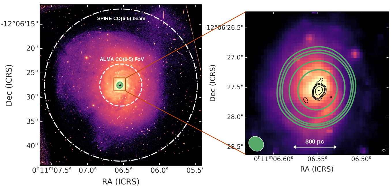
Figure 1: Left panel: HST WFPC2 F606W image of NGC 34 (from Malkan et al. 1998) with superimposed the contours of two ALMA CO(6–5) observations, in green at the resolution of 200 mas, in black of 35 mas. Both the contours are at the respective (3, 4, 5, 10, 20) $\times\,\sigma$, where $\sigma=3.1$ Jy beam^-1 km s^-1 for the green lines and $\sigma=0.27$ Jy beam^-1 km s^-1 for the black lines. The inner white dashed circle indicates the FoV of both ALMA observations, with a radius of 4$\aas@@fstack{\prime\prime}$3 ($\sim$1.7 kpc), while the outer dash-dotted circle represents the Herschel/SPIRE-FTS beam FWHM for CO(6–5) observations, with a 15$\aas@@fstack{\prime\prime}$6 radius. Right panel: zoom of the inner 1 kpc. Restored ALMA beams of the 200 and 35 mas images are shown as ellipses with white edges, at the bottom left (with the green area) and right (with the black area), respectively. The 35 mas ALMA image has not been primary-beam corrected.

In local ($D\sim 1\rm\,Mpc$) sources, the Atacama Large Millimeter Array (ALMA) is able to resolve the morphology of CO emission at $\sim$100 pc scales, from CO(1–0) to the mid-$J$ CO(6–5) line. Higher-$J$ lines, which trace the dense/warm molecular gas possibly influenced by the X-ray photons, fall unfortunately out of the ALMA bands at low redshift. From the ALMA archive we therefore collect all the available maps of the highest possible CO transition – namely the CO(6–5) – for the galaxies in our sample. We use these maps to infer the size of the high-density molecular gas region that cannot be estimated from the Herschel data given their poor spatial resolution. As the critical density of the CO transitions increases with $J$ ($n_{\text{crit}}\propto(J+1)^{3}$), and given that the gas density increases as we get closer to the galaxy center, we expect the higher-$J$ lines to originate from an area extended at most like CO(6–5) (see e.g. Mingozzi et al., 2018). We thus use the typical size of the CO(6–5) emitting region as an upper limit for the AGN sphere of influence on the molecular gas.

Figure 1 shows –as an illustrative example– the spatially resolved CO(6–5) emission from NGC 34, a LIRG in our sample, hosting an obscured ($N_{\text{H}}=10^{23.7}$ cm^-2) AGN (Brightman & Nandra, 2011; Mingozzi et al., 2018). For this source, we retrieved two different ALMA observations, 2011.0.00182.S (PI: Xu) and 2016.1.01223.S (PI: Baba), both carried out in Band 9, where the field of view (FoV) is $\sim$ 8$\aas@@fstack{\prime\prime}$6, but with different spatial resolutions (200 and 35 mas, respectively) and maximum recoverable scales ($2^{\prime\prime}$ and $0.5^{\prime\prime}$, respectively). These scales correspond to 800 and 200 pc at the NGC 34 distance. The total flux of the CO(6–5) detection with a resolution of 200 mas is $S_{\text{CO(6--5)}}=707\pm 106$ Jy km s^-1, obtained by Mingozzi et al. (2018), using CASA 4.5.2 (McMullin et al., 2007) and a natural weighting scheme. This flux, which is shown with the green contours in Figure 1 (see also Xu et al., 2014; Mingozzi et al., 2018), matches that recovered by Herschel/SPIRE within a much larger beam of 31$\aas@@fstack{\prime\prime}$2. This means that this ALMA observation, despite having a smaller FoV with respect to that of SPIRE, recovers all the CO(6–5) emission from the galaxy.

The high-resolution data (project ID 2016.1.01223.S, PI: Baba) are plotted with black contours in Figure 1 and have never been published so far. We used the already calibrated and cleaned data cube from the ALMA Archive. For this data cube, calibration and imaging have been done manually, with a Briggs weighting (robust parameter of 0.5), and passed the QA2 stage. Using CASA 5.6 (McMullin et al., 2007), we produced the moment 0 map from the data cube with the task immoments. To estimate the flux, we performed a 2D Gaussian fit with the task imfit, which returned $62\pm 3$ Jy km s^-1, less than $10\%$ of the total flux measured by SPIRE-FTS ($920\pm 56$ Jy km s^-1). The reason for this discrepancy is that this observation is limited by a much smaller maximum recoverable scale, compared to the 200-mas data. The emission consists of a single clump of $r\lesssim 50$ pc.

In addition to NGC 34, we analysed ALMA CO(6–5) maps available for NGC 1068 (García-Burillo et al., 2014), IRAS F05189–2524 (still unpublished), NGC 5128 (Espada et al., 2017), NGC 5135 (Sabatini et al., 2018), NGC 6240 (still unpublished) and NGC 7130 (Zhao et al., 2016). The images are shown in Appendix B. All these sources are characterized by spatially resolved CO(6–5) emission arising from the galaxy center and extending up to $150-1000$ pc, with median $r=250$ pc. We therefore assume that the bulk of higher-$J$ CO line luminosity – for which we have only Herschel at low resolution – arise from a comparable region of radius $r=250$ pc. In what follows we use this size as an upper limit for $J\geq 6$ transitions emitting region.

3.4 Dust continuum emission as a proxy for star formation

Dust in active galaxies can be heated by both the UV/optical photons coming from black hole accretion, and UV/optical photons associated to star-formation processes (e.g. Hatziminaoglou et al., 2008; Pozzi et al., 2010; Gruppioni et al., 2016). In the first case, the dust is mostly circumnuclear, which means it occupies the central 100 pc at most (e.g. Hickox & Alexander, 2018); in the second case the dust grains reside in the star-forming regions through the galaxy structure. The emission of two dust components peaks at different infrared (IR) wavelengths, due to the different temperatures: the circumnuclear dust ($T\approx 60-100$ K) peaks in the mid-IR, around $10-30\,\mu$m (Alonso-Herrero et al., 2011; Feltre et al., 2012), while the galactic diffuse dust is colder ($T\approx 20-30$ K), peaking in the far-IR around $70\sim 100\,\mu$m (da Cunha et al., 2008).

For this reason we adopt the 70 $\mu$m emission maps from the Herschel Photoconductor Array Camera and Spectrometer (PACS, Poglitsch et al., 2010) as a proxy for SF in our sample galaxies. In this regime the AGN contamination, if any, accounts for a few percent, and the spatial resolution at 70 $\mu$m (FWHM = 5$\aas@@fstack{\prime\prime}$6, corresponding to $\sim$0.17–13 kpc for our sample) is better than at longer wavelengths. We find suitable maps for all the sources, except IRAS 07598+6508, Mrk 463 and PKS 1549-79. We keep anyway these three galaxies in our sample for completeness.

The 5$\aas@@fstack{\prime\prime}$6 spatial resolution allows us to map the distribution of SF, assuming that all the 70 $\mu$m photons trace the original stellar UV radiation. From visual inspection, SF is occurring mostly in the central regions ($r\sim 2$ kpc) of our galaxies. The procedure to extract the star formation rate (SFR) and the radial profile of the Habing field from the 70 $\mu$m data is outlined in Section 5.1.

3.5 Low-J CO data

To complete the CO SLEDs observations from Herschel discussed in Section 3.2, we collect (see Table 2) the low-$J$ fluxes available in the literature, from CO(1–0) to CO(3–2). These transitions have been observed using several single-dish telescopes: the 14-m Five College Radio Astronomy Observatory (FCRAO), the 15-m Swedish-ESO Submillimeter Telescope (SEST), the 30-m Institut de Radioastronomie Millimétrique Pico Veleta telescope (IRAM-30m), the 12-m Atacama Pathfinder Experiment (APEX), and the 15-m James Clerk Maxwell Telescope (JCMT).

We expect these low-$J$ CO lines to trace a larger area than mid-$J$ and high-$J$ lines, since they are characterized by lower $n_{\text{crit}}$ and lower excitation temperatures. CO(1–0) is especially important since its flux is the most widely used proxy for the total molecular gas mass of a galaxy (Bolatto et al., 2013). For the closest galaxies, their projection on the sky could result larger than the telescope collecting area. For this reason, when multiple observations are available, we prioritize mosaics and larger beams.

Many authors have found that CO(1–0) emitting gas has a exponential radial profile, and that there is a relation between the CO(1–0) scale length $r_{\text{CO}}$ and the optical radius $r_{25}$ (Leroy et al., 2008; Schruba et al., 2011; Villanueva et al., 2021). Since the $\sim\!30\%$ of our sample contains highly inclined galaxies ($i\geq 60^{\circ}$), we follow Boselli et al. (2014) and Casasola et al. (2020) assuming that the CO(1–0) emission is well described by an exponential decline both along the radius $r$ and above the galactic plane on the $z$ direction (3D method):

$$S_{\text{CO}}(r,z)=S_{\text{CO,tot}}e^{-r/r_{\text{CO}}}e^{-|z|/z_{\text{CO}}}\,,$$ (1)

where $r_{\text{CO}}=0.17\,r_{25}$ and $z_{\text{CO}}=0.01\,r_{25}$, as in Casasola et al. (2017) and Boselli et al. (2014). We stress that for galaxies with low inclination, the 3D method is analogous to the standard 2D approach, such as that developed by Lisenfeld et al. (2011). The adopted approach provides a median $r_{\text{CO}}=3.07^{+2.06}_{-1.48}$ kpc for our sample.

4 CO emission on global galactic scales

Before investigating the PDR vs. XDR contribution to the molecular gas heating in the center of our sample galaxies, we want to see if, on the scale of the whole galaxy, it is already possible to see the influence of the AGN on the molecular gas phase. We check how our active galaxies compare to other active and non-active samples on the Schmidt–Kennicutt plane (Schmidt, 1959; Kennicutt, 1998), which links the molecular gas surface density $\Sigma_{\text{mol}}$ and the SFR surface density $\Sigma_{\text{SFR}}$, i.e. the star formation to its fuel.

We calculate the surface densities $\Sigma_{\text{mol}}$ and $\Sigma_{\text{SFR}}$ within the CO radius r${}_{\text{CO}}$, defined as a fraction of the optical radius $r_{25}$ (see Section 3.5). We derive the molecular mass from the CO(1–0) flux in the following way. For each source, we have the CO(1–0) flux $S_{\text{CO}}$, measured within the telescope beam, with FWHM $2\theta$, in angular units (the factor 2 is due to the fact that the FWHM is a diameter, while we want a radius). In spatial units (e.g. in pc) in the source reference frame, this corresponds to a radius $r_{\theta}$, so that the flux recovered by the telescope is:

$$S_{\text{CO}}(r_{\theta})=\iint_{0}^{r_{\theta}}S_{\text{CO}}drdz=S_{\text{CO,tot}}(e^{-r_{\theta}/r_{\text{CO}}}-1)(e^{-r_{\theta}/z_{\text{CO}}}-1).$$ (2)

If we put $r_{\text{CO}}$ instead of $r_{\theta}$ in Equation 2, we obtain that $S_{\text{CO}}(r_{\text{CO}})\approx 0.63S_{\text{CO,tot}}$. Given that we know $S_{\text{CO}}(r_{\theta})$ from observations, we can calculate the CO(1–0) flux within $r_{\text{CO}}$:

$$S_{\text{CO}}(r_{\text{CO}})=\iint_{0}^{r_{\text{CO}}}S_{\text{CO}}(r,z)drdz=\frac{0.63\,S_{\text{CO}}(r_{\theta})}{(e^{-r_{\theta}/r_{\text{CO}}}-1)(e^{-r_{\theta}/z_{\text{CO}}}-1)}$$ (3)

We find a median ratio $S_{\text{CO}}(r_{\text{CO}})/S_{\text{CO}}(r_{\theta})=0.70^{+0.30}_{-0.06}$, with only one galaxy (NGC 5128) having $S_{\text{CO}}(r_{\text{CO}})/S_{\text{CO}}(r_{\theta})>2$. From the CO(1–0) flux calculated within $r_{\text{CO}}$, we estimate the molecular mass by using the following equation from Bolatto et al. (2013):

$$M_{\text{mol}}=1.05\times 10^{-16}X_{\text{CO}}\frac{S_{\text{CO}}D^{2}_{\text{L}}}{1+z}\,M_{\odot}\,,$$ (4)

where $S_{\text{CO}}$ is the CO(1–0) flux in Jy km s^-1, $D_{\text{L}}$ is the luminosity distance in Mpc, $z$ is the redshift, and $X_{\text{CO}}$ is the CO-to-H₂ conversion factor. The masses thus calculated already take into account the contribution of helium and heavy elements. To line up with the other samples included in our comparison, we adopt a Milky Way value of $X_{\text{CO}}=2\times 10^{20}$ cm^-2 (K km s^-1)^-1, corresponding to $\alpha_{\text{CO}}=4.3$ M_⊙ (K km s^-1 pc^-2)^-1, defined as the mass-to-light ratio between $M_{\text{mol}}$ and the CO(1–0) luminosity.

We find $M_{\text{mol}}$ between $10^{7.4}$ and $10^{10.6}$ M_⊙, with median $\log(M_{\text{mol}}/M_{\odot})=10.1^{+0.3}_{-0.7}$. These $M_{\text{mol}}$ are calculated within $r_{\text{CO}}$: to extrapolate the results to the whole galaxy ($r\rightarrow+\infty$), a multiplicative factor of $1/0.63$ is needed. The molecular masses calculated using Equations 3 and 4 are reported in Table 1, while the uncorrected (i.e. the observed) CO luminosities are the ones in Table 2. We note that these masses could be upper limits, since we are adopting a Milky Way value of $\alpha_{\text{CO}}$, while it is thought that dusty (U)LIRGs and starburst galaxies have a lower $\alpha_{\text{CO}}\approx 0.8$ M_⊙ (K km s^-1 pc^-2)^-1 (Downes & Solomon, 1998; Bolatto et al., 2013).

The SFRs are estimated from the radial profile $F_{70}(r)$ of the 70 $\mu$m photometry maps: $\log\text{SFR}=\log L_{70}-43.23$ (Calzetti et al., 2010; Kennicutt & Evans, 2012), where $L_{70}$ is in units of erg s^-1 and comes from the integration of $F_{70}(r)$ up to r${}_{\text{CO}}$. This SFR calibration depends on the quantity of dust (it works better for dusty starburst galaxies) and the stellar population mix, and works better for galaxies with $L_{70}>4.4\times 10^{9}$ L_⊙ (Calzetti et al., 2010), which is satisfied by the $\sim 90\%$ of our galaxies. Using this SFR calibration, we find a median SFR $=12.5^{+34.9}_{-9.8}$ M_⊙ yr^-1.

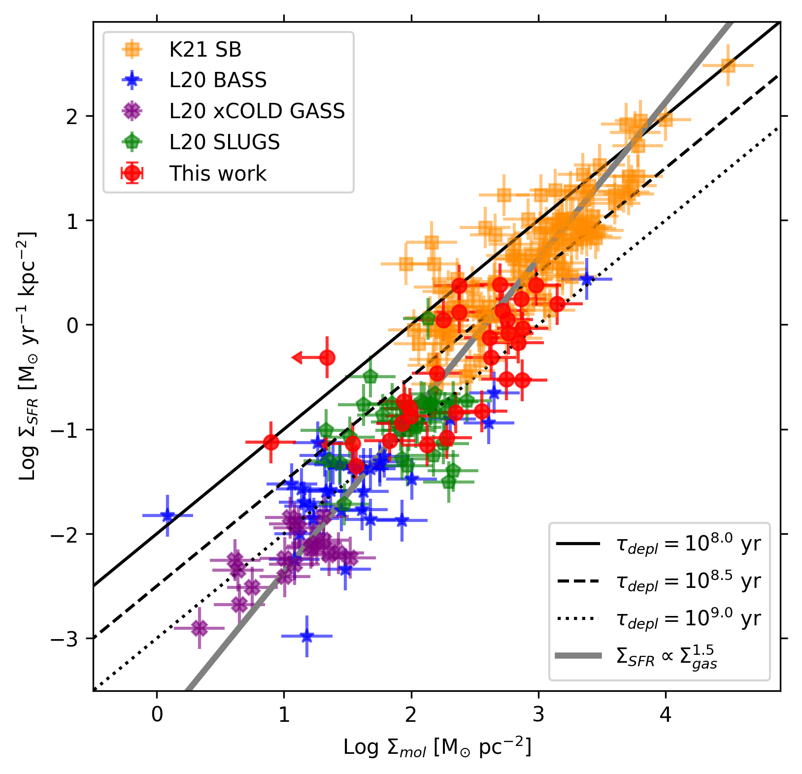
Figure 2: Schmidt–Kennicutt relation for our sample of active galaxies (red circles), the starburst sample from Kennicutt & De Los Reyes 2021 (orange squares), and the AGN sample (blue stars) and normal SFG (pink crosses and green pentagons) from Lamperti et al. (2020). Lines of constant molecular gas depletion times are overlayed to the data. The gray solid line is the best fit for a single relation as reported by Kennicutt & De Los Reyes (2021), namely $\log\Sigma_{\text{SFR}}=1.5\log\Sigma_{\text{mol}}-3.87$. All molecular surface densities were derived using the Milky Way value $\alpha_{\text{CO}}=4.3$ M_⊙ (K km s^-1 pc^-2)^-1.

In Figure 2, we show our galaxies in the $\Sigma_{\text{mol}}$ – $\Sigma_{\text{SFR}}$ plane, comparing them with starburst (SB) galaxies from Kennicutt & De Los Reyes 2021 (K21, hereafter), AGN observed with Swift/BAT from the BASS sample (Ricci et al., 2017a), star-forming galaxies (SFG) from the xCOLD GASS survey (Saintonge et al., 2017), and IR luminous galaxies from SLUGS (Dunne et al., 2000). The latter three samples were gathered by Lamperti et al. 2020 (L20, hereafter).

Our estimates of $\Sigma_{\text{mol}}$ and $\Sigma_{\text{SFR}}$ mainly depend on the assumed CO exponential profile and the SFR–70 $\mu$m calibration. Following K21, we assign a conservative error of $\pm 20\%$ to both $\Sigma_{\text{mol}}$ and $\Sigma_{\text{SFR}}$. Since we could not recover the data errors from every point of L20, we adopt the same $\pm 20\%$ uncertainty also for their points.

We want to see if there is a difference between normal SFGs and AGN on the $\Sigma_{\text{mol}}-\Sigma_{\text{SFR}}$ plane. As shown in Figure 2, our sample of AGN fit well in between the starburst galaxies of K21 and the mixed (AGN/SFGs) sources from L20. We note a gap between the K21 and L20 sources, probably due to the difference in the area assumed for deriving the surface densities: K21 calculate a circumnuclear starburst region differently for every galaxy, finding $r=2.8^{+3.3}_{-1.2}$ kpc; L20 instead use the CO observation beam area, which has a FWHM of 15 arcsec for the SLUGS sample and $20\sim 22$ arcsec for both the xCOLD GASS and the BASS sample (hence radii of $0.4\sim 11$ kpc). Overall, we find that, on the kpc-scale, an AGN effect on the SF is not evident, thus confirming earlier findings from Lamperti et al. (2020), and from Casasola et al. (2015), who studied the Schmidt–Kennicutt relation for four AGN from the NUGA sample (García-Burillo et al., 2003).

In Fig. 2 we highlight the lines corresponding to constant depletion time, $\tau_{\text{depl}}=\Sigma_{\text{mol}}/\Sigma_{\text{SFR}}=[10^{8},10^{8.5},10^{9}]$ yr, respectively. For the galaxies in our sample, we find a median $\log(\tau_{\text{depl}}/\text{yr})=8.9^{+0.4}_{-0.6}$, similar to other studies of Seyferts (e.g. Salvestrini et al., 2020), and slightly lower than typical values for local inactive SFGs (Bigiel et al., 2008; Utomo et al., 2018; Leroy et al., 2021, all find a median $\tau_{\text{depl}}\sim 2\times 10^{9}$ yr). Conversely, typical progenitors of ellipticals or proto-spheroids galaxy models (Calura et al., 2014) require $\tau_{\text{depl}}\sim 2\times 10^{7}$ yr, while dusty sub-millimeter galaxies (SMG), which are mostly hyperluminous infrared galaxies (HyLIRG, $L_{\text{IR}}\geq 10^{13}$ L_⊙) at moderately high redshift ($z\sim 3$) can have even shorter $\tau_{\text{depl}}\leq 10^{7}$ yr (Carilli & Walter, 2013), but these are probably extreme and rare objects (Heckman & Best, 2014).

From a classical evolutionary perspective, active, interacting (U)LIRGs are thought to be an intermediate stage between a late-type SFG and a quiescent early-type galaxy (Hopkins et al., 2008). From more recent works it seems that interacting and merging systems can account only for the formation of the most massive ellipticals, while slow secular processes (in the local Universe) or rapid instabilities in clumpy gaseous disks (at high $z$) are responsible for the evolution of the bulk of the galaxies (Heckman & Best, 2014). Within the limits of our analysis, we do not see a strong effect of AGN feedback on $\tau_{\text{depl}}$ at kpc-scales, but that its impact also depends on the choice of $\alpha_{\text{CO}}$.

5 CO emission in the galaxy centers

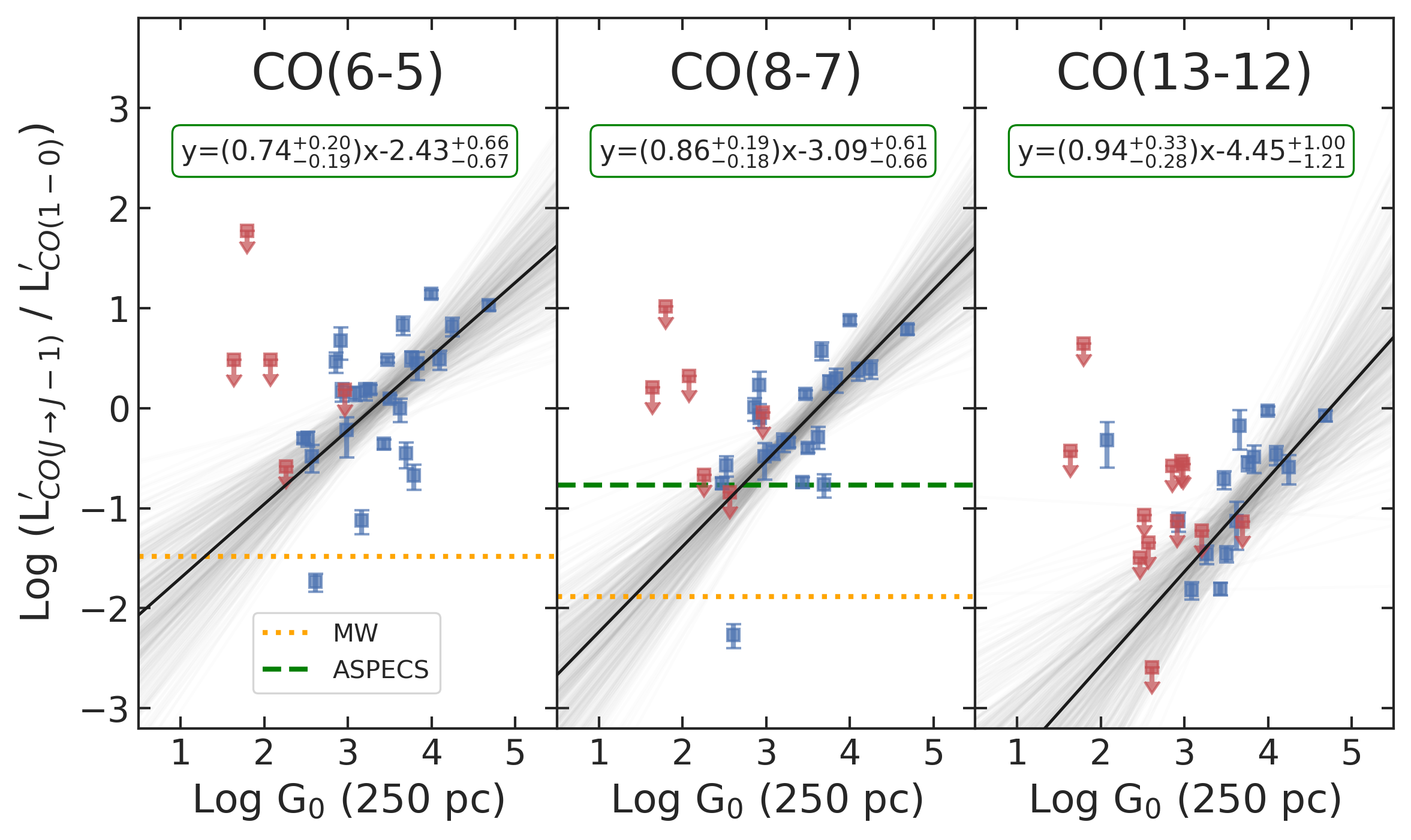
(a)

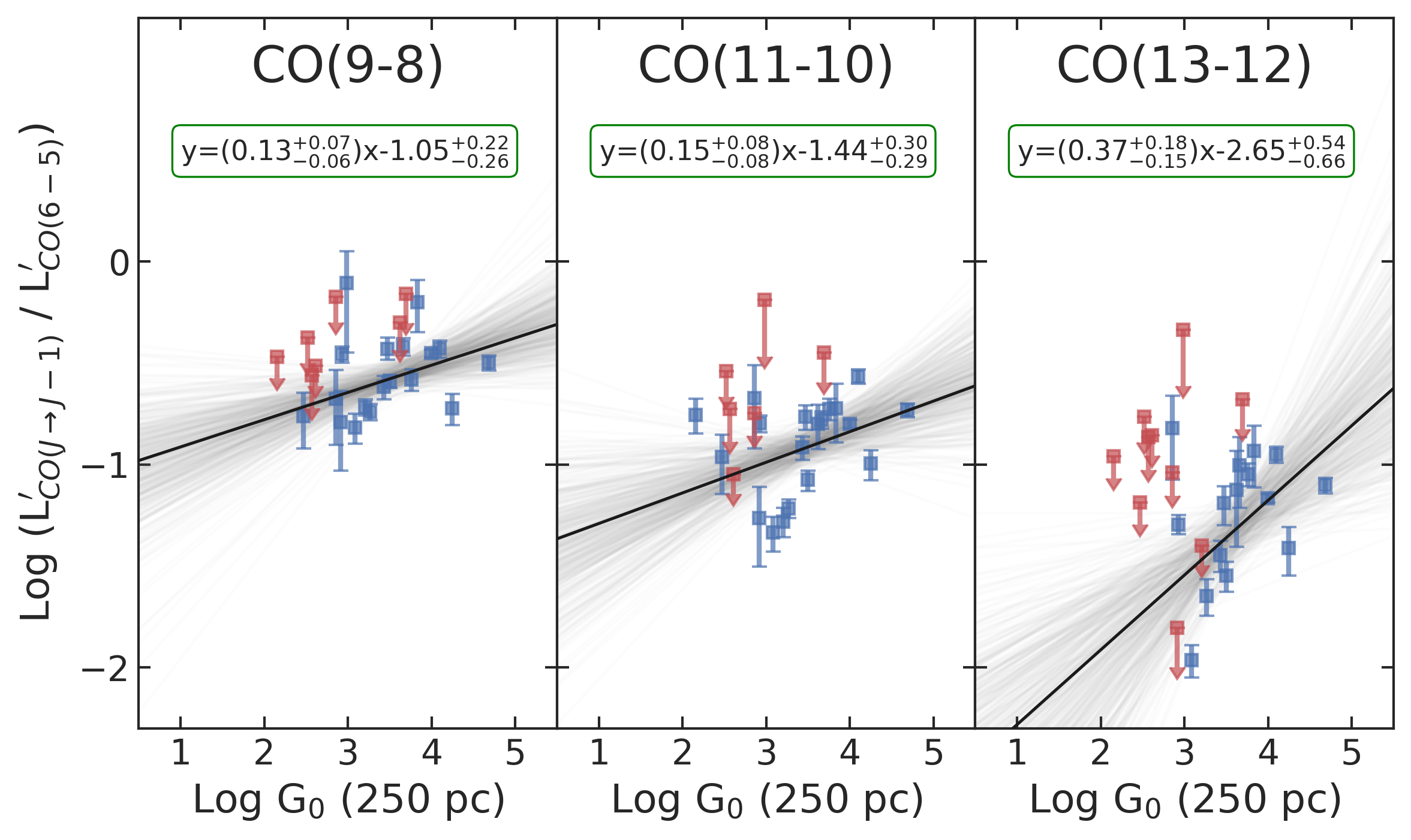
(b)

Figure 3: CO line ratios as a function of the Habing field, $G_{0}$, measured at $r=250$ pc (see Section 5.1). We consider both the luminosity ratios $L^{\prime}_{\text{CO}(J\rightarrow J-1)}/L^{\prime}_{\text{CO}(1\rightarrow 0)}$ with respect to the CO(1–0) (left panel, 3(a)) and $L^{\prime}_{\text{CO}(J\rightarrow J-1)}/L^{\prime}_{\text{CO}(6\rightarrow 5)}$ with respect to the CO(6–5) line luminosity (right panel, 3(b)). The luminosities $L^{\prime}$ are in units of K km s^-1 pc^-2, and $J$ is indicated on the top of each panel. Blue squares indicate $3\sigma$ detections, while red squares with downward arrow indicate $<3\sigma$ detections in the higher-$J$ line (i.e. censored data). The solid black line is the regression fit, with the underlying grey lines showing the fits drawn from the posterior distribution. When available, the Milky Way (dotted orange line, data from Fixsen et al. 1999) and the ASPECS AGN (green dashed line, data from Boogaard et al. 2020) CO ratios are also shown.

We now focus on the CO emission in the inner 500 pc (i.e. up to $r=250$ pc from the center) with the aim of assessing the relative contribution of PDR and/or XDR to the molecular gas in the vicinity of the AGN. To this goal, we exploit the line ratios with respect to CO(1–0) and CO(6–5): $L^{\prime}_{\text{CO}(J\rightarrow J-1)}/L^{\prime}_{\text{CO}(1-0}$ (i.e. high-$J$/low-$J$ ratios) and $L^{\prime}_{\text{CO}(J\rightarrow J-1)}/L^{\prime}_{\text{CO}(6-5)}$ (i.e. high-$J$/mid-$J$ ratios), where all $L^{\prime}_{\text{CO}}$ are in units of K km s^-1 pc^-2. We use the CO(1–0) theoretical profile (Equation 3) to calculate the flux within $r=250$ pc:

$$S_{\text{CO}}(r\leq 250\text{ pc})=S_{\text{CO,tot}}(e^{-250\text{pc}/r_{\text{CO}}}-1)(e^{-250\text{pc}/z_{\text{CO}}}-1)$$ (5)

Conversely, we do not correct the other CO lines: we know (Section 3.3) that CO(6–5) emission is mostly confined within the central 250 pc, and the same should likely apply for higher-$J$ lines. There are few studies that map the size of other low-$J$ lines than CO(1–0): Casasola et al. (2015) compares CO(1–0), CO(2–1) and CO(3–2) images for 4 nearby active galaxies (none of which is part of this sample), finding a similar physical size for the first two transitions and a halved size (mean $\sim 500$ pc) for the available CO(3–2) maps; NGC 1068, however, has a CO(3–2) emission which extends beyond the central 2 kpc (García-Burillo et al., 2014). Among our sample of galaxies, Dasyra et al. (2016) have published a CO(4–3) image of IC 5063, which has a similar size ($\sim 1$ kpc) of its CO(2–1) emission. CO(4–3) images of IRAS F05189–2524, NGC 5135, ESO 286–IG019, NGC 7130, NGC 7469 and ESO 148–IG002, among other (U)LIRGs, are published by Michiyama et al. (2021), who find emitting sizes for the aforementioned galaxies between 1 and 5 kpc. Since these low-$J$ CO transitions are not the focus of the present work, and since we do not have a theoretical radial profile to correct them, we leave them unaltered, and put the relative plots only in the Appendix A.

In the next two subsections, we derive the fluxes of FUV and X-ray photons, which are the heating drivers in PDRs and XDRs, respectively, and we compare them with the CO line ratios.

5.1 PDR

The FUV flux (also often referred to as interstellar radiation field) is measured in Habing units $G_{0}$, where $G_{0}=1$ corresponds to its value in the solar neighbourhood: $1.6\times 10^{-3}$ erg cm^-2 s^-1 in the FUV band (Habing, 1968). As discussed in Section 3.4, the FUV photons are efficiently absorbed by dust grains, which re-emit energy in the infrared (IR), especially around 70$\mu$m (given typical dust temperatures; da Cunha et al., 2008). Since our systems are powerful IR-emitters (with median $\log(L_{\text{IR}}/L_{\odot})=11.4^{+0.6}_{-0.9}$), we assume that all the FUV photons are processed by dust and re-emitted at 70 $\mu$m.

We use Herschel/PACS 70 $\mu$m High Level Images to extract a value for $G_{0}$, assuming that all FUV photons are absorbed by dust grains and re-emitted at 70 $\mu$m. To do so, we fit the radial profile of the 70 $\mu$m photometric map with a Sersic function:

$$F(R)=F_{e}\exp\left\{-b_{n}\left[\left(\frac{R}{R_{e}}\right)^{1/n}-1\right]\right\}.$$ (6)

The free parameters of this fit are $F_{e}$, $R_{e}$ and $n$, while $b_{n}$ is a constant that depends on $n$ (Sérsic, 1963). We then divide the normalization flux $F_{e}$ by $1.6\times 10^{-3}$ erg cm^-2 s^-1, obtaining a profile in $G_{0}$ units. In this way we find values corresponding to the radius $R_{e}$, with median $\log G_{0}(R_{e})=2.6^{+0.5}_{-0.8}$, which is similar to what Farrah et al. (2013) and Díaz-Santos et al. (2017) found for local (U)LIRGs, in the HERUS ($10^{2.2}<G_{0}<10^{3.6}$) and the GOALS ($10^{1}<G_{0}<10^{3.5}$) samples, respectively. It is important to note that in these works, as in most of the literature, $G_{0}$ is derived from PDR calculations fitting the observed line emission, thus relying on PDR codes as e.g. the PDR Toolbox (Pound & Wolfire, 2008) and Cloudy (Ferland et al., 2017). Here, instead, we observationally derive $G_{0}$ and we use the fitted profile to estimate its value at different radii. $G_{0}$ increases at smaller radii due to the higher SFR in the circumnuclear region, and the consequent high FUV irradiation. At $r=250$ pc, we find a median $\log G_{0}(250\text{pc})=3.1^{+0.7}_{-0.8}$. We look then for correlations between the CO line ratios and $G_{0}$ (from now on when we refer to $G_{0}$ values we mean measured at $r=250$ pc), to understand if the FUV irradiation can explain by itself the observed CO emission at the center of local active galaxies.

In Figure 3 we show the CO(6–5)/CO(1–0), CO(8–7)/CO(1–0), and CO(13–12)/CO(1–0) luminosity ratios on the left panel, and the CO(9–8)/CO(6–5), CO(11–10)/CO(6–5) and CO(13–12)/CO(6–5) ratios on the right panel, as a function of $G_{0}$. All the other CO line ratios are presented in the Appendix A. We see an overall trend, for high-$G_{0}$ galaxies, to show increasing high-$J$/low-$J$ and high-$J$/mid-$J$ ratios.

We fit a regression line with the Linmix algorithm (Kelly, 2007), which evaluates the likelihood in presence of censored data (i.e. upper limits). Linmix computes the likelihood function by convolving multiple (we use two, since adding more has a negligible effect on our results) hierarchical Gaussian distributions. We also tried to fit only the detections with an ordinary least squares regression and with a bootstrapped version of the same algorithm, finding limited differences with respect to the Linmix regression, which includes the censored data. Since an important fraction (between 20 and 50 $\%$, depending on the transition) of the high-$J$ CO fluxes are actually upper limits (see Table 2), we plot the Linmix results in Figures 3 and 4 and in Appendix A.

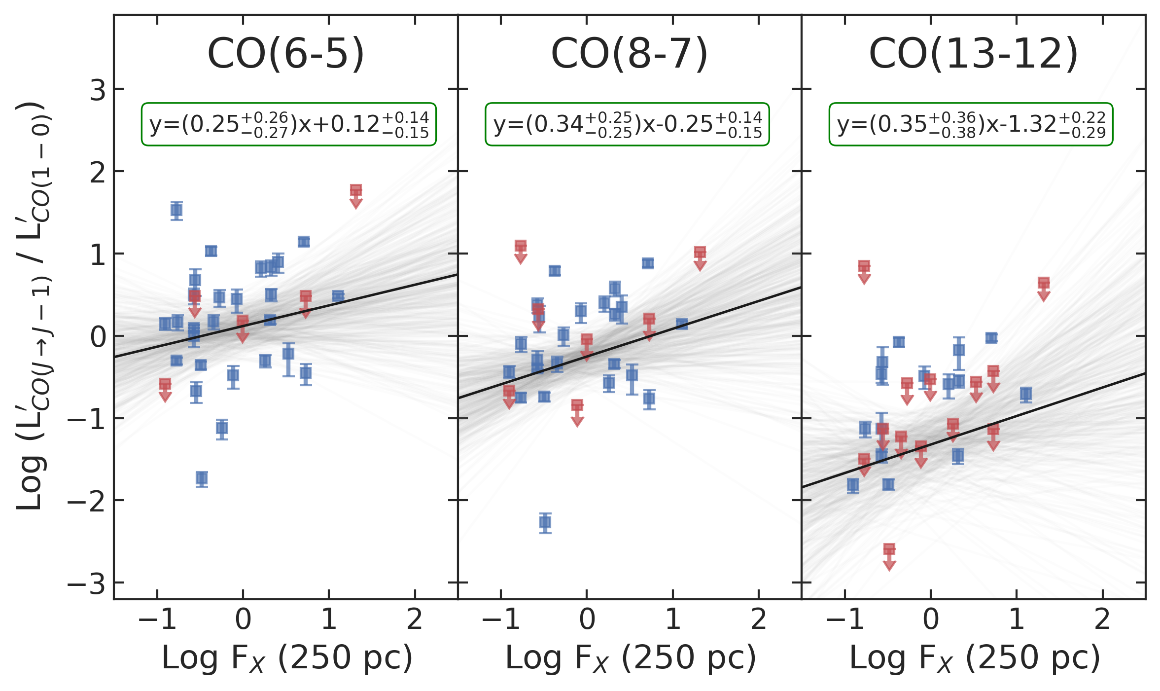
(a)

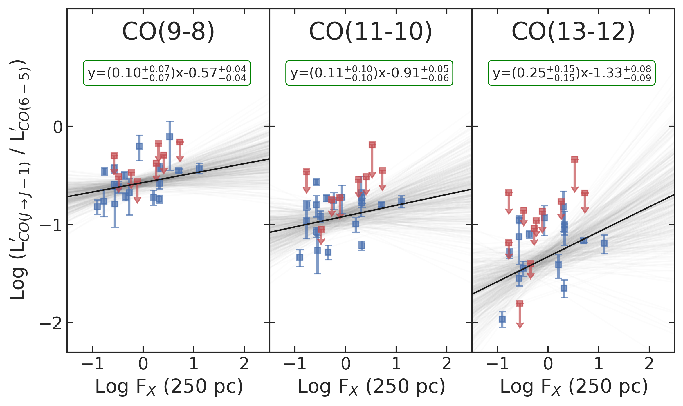
(b)

Figure 4: CO ratios as a function of $F_{\text{X}}$, in units of erg s^-1 cm^-2, derived at $r=250$ pc (see Section 5.2). We consider both the luminosity ratios $L^{\prime}_{\text{CO}(J\rightarrow J-1)}/L^{\prime}_{\text{CO}(1\rightarrow 0)}$ with respect to the CO(1–0) (left panel, 4(a)) and $L^{\prime}_{\text{CO}(J\rightarrow J-1)}/L^{\prime}_{\text{CO}(6\rightarrow 5)}$ with respect to the CO(6–5) line luminosity (right panel, 4(b)). The luminosities $L^{\prime}$ are in units of K km s^-1 pc^-2, and $J$ is indicated on the top of each panel. Blue squares indicate $3\sigma$ detections in both lines; red squares with downward arrow indicate $<3\sigma$ detections in the higher-$J$ line. The solid black line is the regression fit, with the underlying grey lines showing the fits drawn from the posterior distribution.

We find steeper slopes for the CO(1–0) ratios, and a trend of increasing steepness with $J$ for both ratios. However, almost all the regression slopes return a sub-linear relation between the CO line ratios and $G_{0}$, with slopes $0.3-1.1$ for the CO(1–0) ratios, and $0.1-0.4$ for the CO(6–5) ratios. These findings suggest that the CO excitations are not strongly dependent on the radiative field $G_{0}$, and other excitation mechanisms may contribute to the CO line emission.

We also plot in Figure 3 the median line ratios for the Milky Way (Fixsen et al., 1999, MW,) and the AGN from the ASPECS (Walter et al., 2016) AGN sample (Boogaard et al., 2020). The MW has a lower CO ratio than most of our sources, which is expected since our galaxies are forming stars at a higher rate than the MW and host an AGN. The ASPECS AGNs are instead bright (L${}_{\text{IR}}\sim 10^{12}L_{\odot}$) and have a median CO ratio comparable to our active galaxies. These AGN are located at $z\sim 1-3$, at the peak of the cosmic SF history (Madau & Dickinson, 2014).

5.2 XDR

We use the $L_{X}$ and $N_{H}$ derived for our sample (see Section 3.1 for details) to estimate the unobscured X-ray flux, $F_{X}=L_{X}/(4\pi r^{2})$, illuminating the GMCs located at $r=250$ pc from the center of our galaxies. We find a median $\log(F_{\text{X}}/\text{erg s}^{-1}\text{cm}^{-2}))=-0.1_{-0.5}^{+0.8}$.

According to theoretical (Kawakatu & Wada, 2008) and observational works (Davies et al., 2007; Esquej et al., 2014; Motter et al., 2021), the circumnuclear star-forming region directly influenced by the AGN has a $\approx 100$ pc radius. However, with the available ALMA data (Section 3.3) we could study only up to the mid-$J$ CO(6–5) emission, which is confined, on average, within a $\sim 250$ pc radius. We, therefore, calculate our X-ray fluxes at this $r=250$ pc. It is also possible to estimate $F_{X}$ from XDR numerical modelling, as done by van der Werf et al. (2010); Pozzi et al. (2017); Mingozzi et al. (2018). Those works all find higher $F_{\text{X}}$ than ours for three galaxies of our sample (respectively Mrk 231, NGC 7130, and NGC 34). This may imply that $r=250$ pc is a too large radius for the central XDR.

The X-ray flux $F_{\text{X}}$ does not account for the obscuration of the X-ray photons before they strike the molecular gas. It is therefore useful to calculate the local (i.e. accounting for the absorption) X-ray energy deposition rate per particle $H_{\text{X}}$. It can be estimated from the following formula (Maloney et al., 1996):

$$H_{\text{X}}\approx 7\times 10^{-22}L_{44}\,r_{2}^{-2}N_{22}^{-1}\;\;\text{erg s}^{-1},$$ (7)

where the X-ray luminosity is $L_{X}=10^{44}L_{44}$ erg s^-1, the distance to the X-ray source is $r=10^{2}r_{2}$ pc and the attenuating column density is $N_{H}=10^{22}N_{22}$ cm^-2. We find a median $\log(H_{\text{X}}/(\text{erg s}^{-1})=-25.3^{+1.1}_{-0.9}$. We use the $N_{\text{H}}$ measured from the X-ray spectrum (Section 3.1) to estimate $H_{\text{X}}$. Although a Compton-thick gas ($N_{\text{H}}>10^{24}$ cm^-2) is generally associated to small-scale structures like a dusty molecular torus, Compton-thin gas (as it is for $65\%$ of our sample) may be part of the same circumnuclear gas we are studying from molecular and IR emission (Ballantyne, 2008; Hickox & Alexander, 2018). In this case, the $H_{\text{X}}\propto N_{\text{H}}^{-1}$ we calculate from Equation 7 could be underestimated, since there would be a lower $N_{\text{H}}$ between the XDR and the AGN.

A key physical quantity affecting the XDR emission, and directly proportional to $H_{\text{X}}/n$, is the effective ionization parameter, defined (Maloney et al., 1996; Galliano et al., 2003; Motter et al., 2021) as:

$$\xi_{\text{eff}}=1.06\times 10^{-2}L_{44}\,r_{2}^{-2}\,N_{22}^{-\alpha}\,n_{5}^{-1}\;\;\text{erg cm}^{3}\text{ s}^{-1},$$ (8)

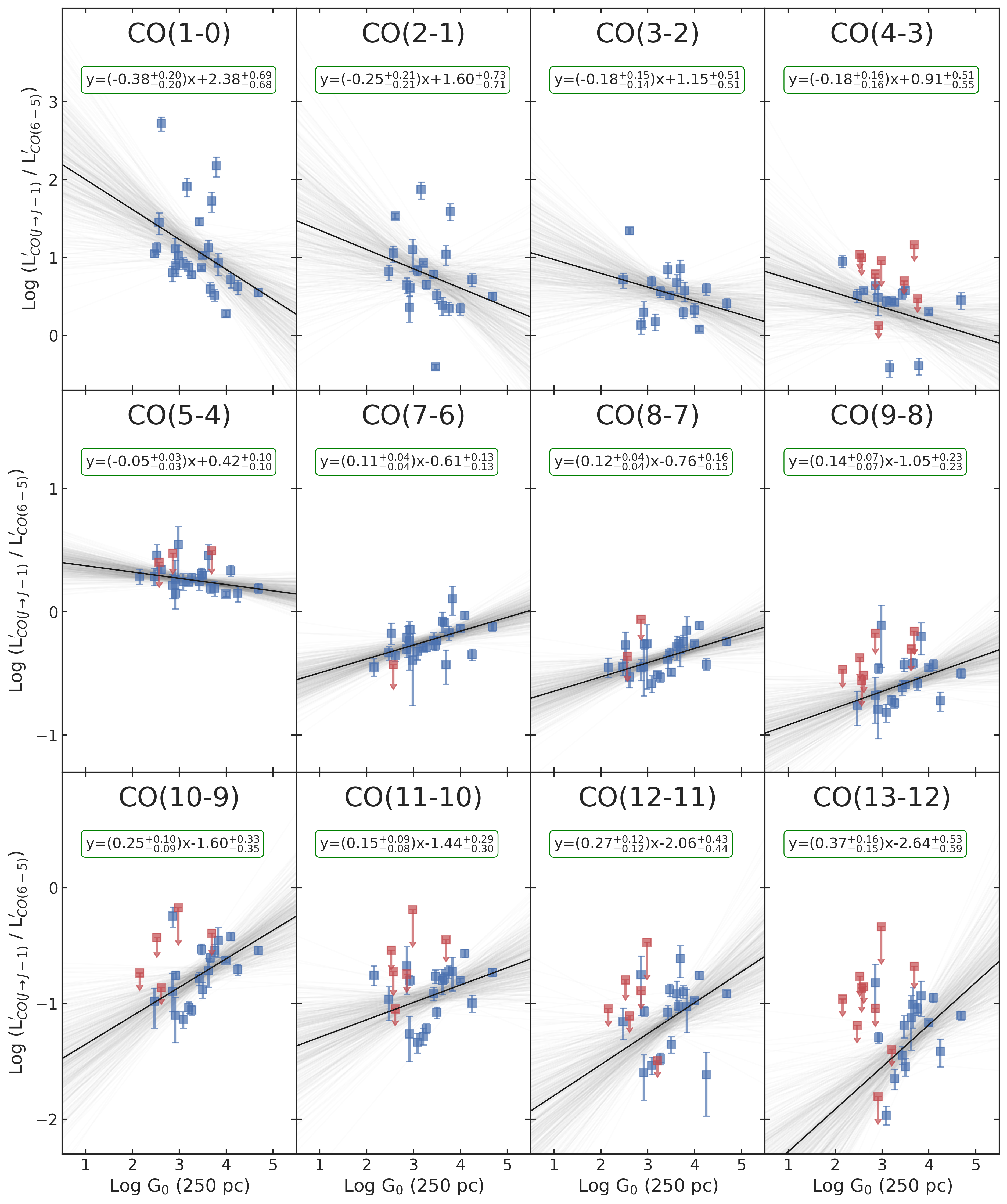
Figure 7: CO line ratios, with respect to the CO(6–5) line, vs. $G_{0}$. The $x$-axis is the Habing field $G_{0}$ (for $r=250$ pc). The $y$-axis is the luminosity ratio $L^{\prime}_{\text{CO}(J\rightarrow J-1)}/L^{\prime}_{\text{CO}(6\rightarrow 5)}$ to the CO(6–5) line. Data points and lines are described in Figure 6.

where the density of the XDR gas is $n=10^{5}n_{5}$ cm^-3, $\alpha=(\Gamma+2/3)/(8/3)$ depends on the photon index $\Gamma$ of the X-ray spectrum (Kawamuro et al., 2020) and the other quantities are the same defined above for $H_{\text{X}}$. For a representative fixed value of $n_{5}=0.1$ we find a median $\log\xi_{\text{eff}}/(\text{erg cm}^{3}\text{s}^{-1})=-4.2^{+1.9}_{-1.0}$. These values are very low when compared to the theoretical values found in Maloney et al. (1996) models (e.g. their Figure 7) and to the observed values found in Motter et al. (2021), who calculated $\xi_{\text{eff}}$ for the active galaxy NGC 34, also present in our sample. Motter et al. (2021) used $N_{\text{H}}$ derived from radio observations (which is 1 dex lower than the one we use for NGC 34, derived from X-rays), and calculated $\xi_{\text{eff}}$ at distances from the AGN between 40 and 120 pc, thus finding values $\sim\!2$ dex higher than us. When taking into account these differences, the results are compatible. Again, this may be a clue that at $r=250$ pc we cannot yet see the AGN impact.

In Figure 4 we plot the same luminosity line ratios (CO(6–5)/CO(1–0), CO(8–7)/CO(1–0) and CO(13–12)/CO(1–0) on the left panel, CO(9–8)/CO(6–5), CO(11–10)/CO(6–5) and CO(13–12)/CO(6–5) on the right panel) analysed in Figure 3, as a function of $F_{\text{X}}$ only, since both $H_{\text{X}}$ and $\xi_{\text{eff}}$ were showing, compared to $F_{\text{X}}$, less defined trends. The other CO line ratios and their regression fits, as function of $F_{\text{X}}$, are presented in Appendix A.

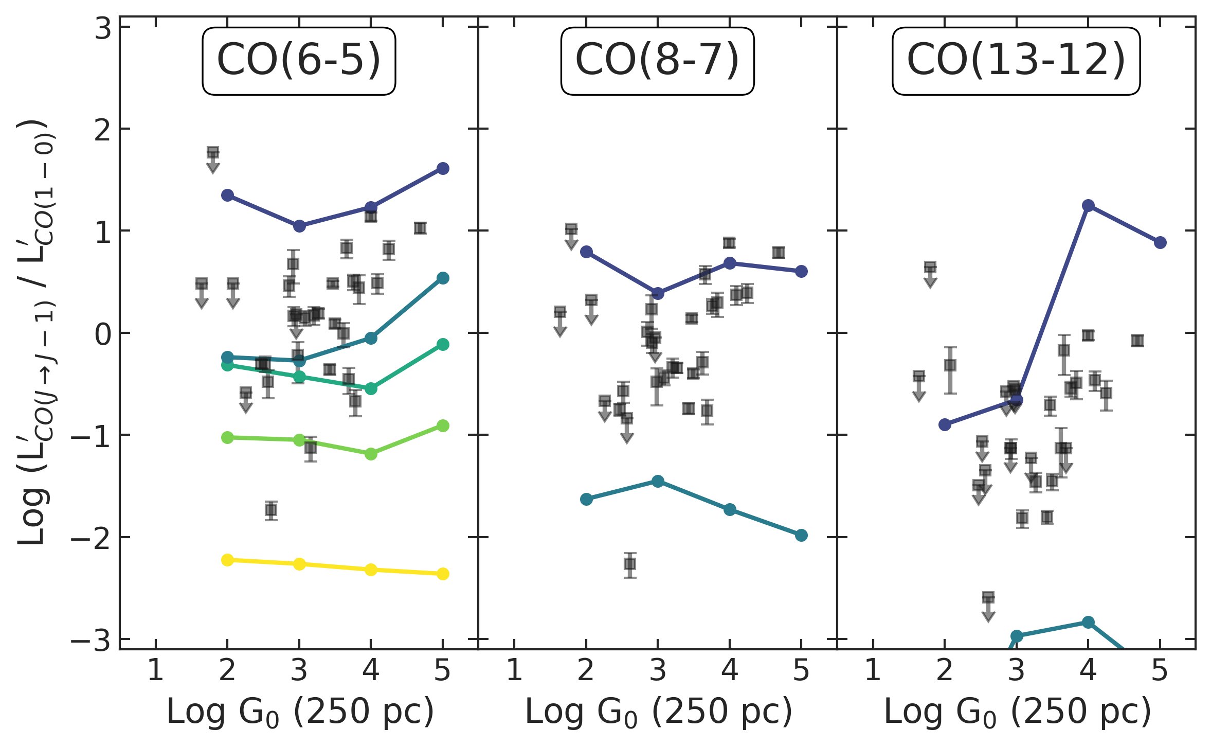
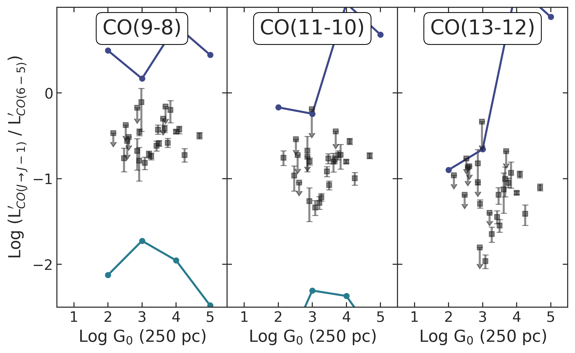
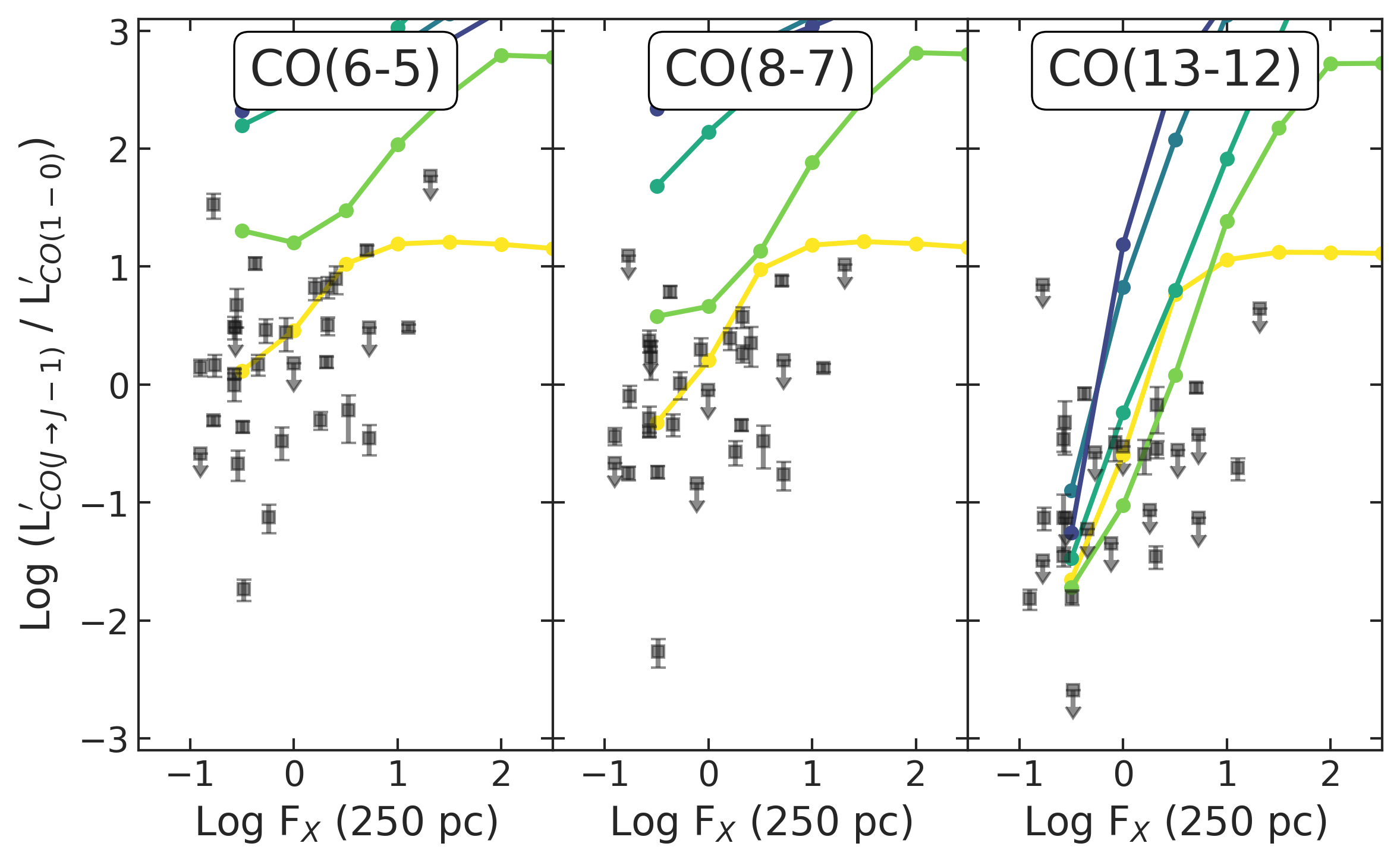
(a)

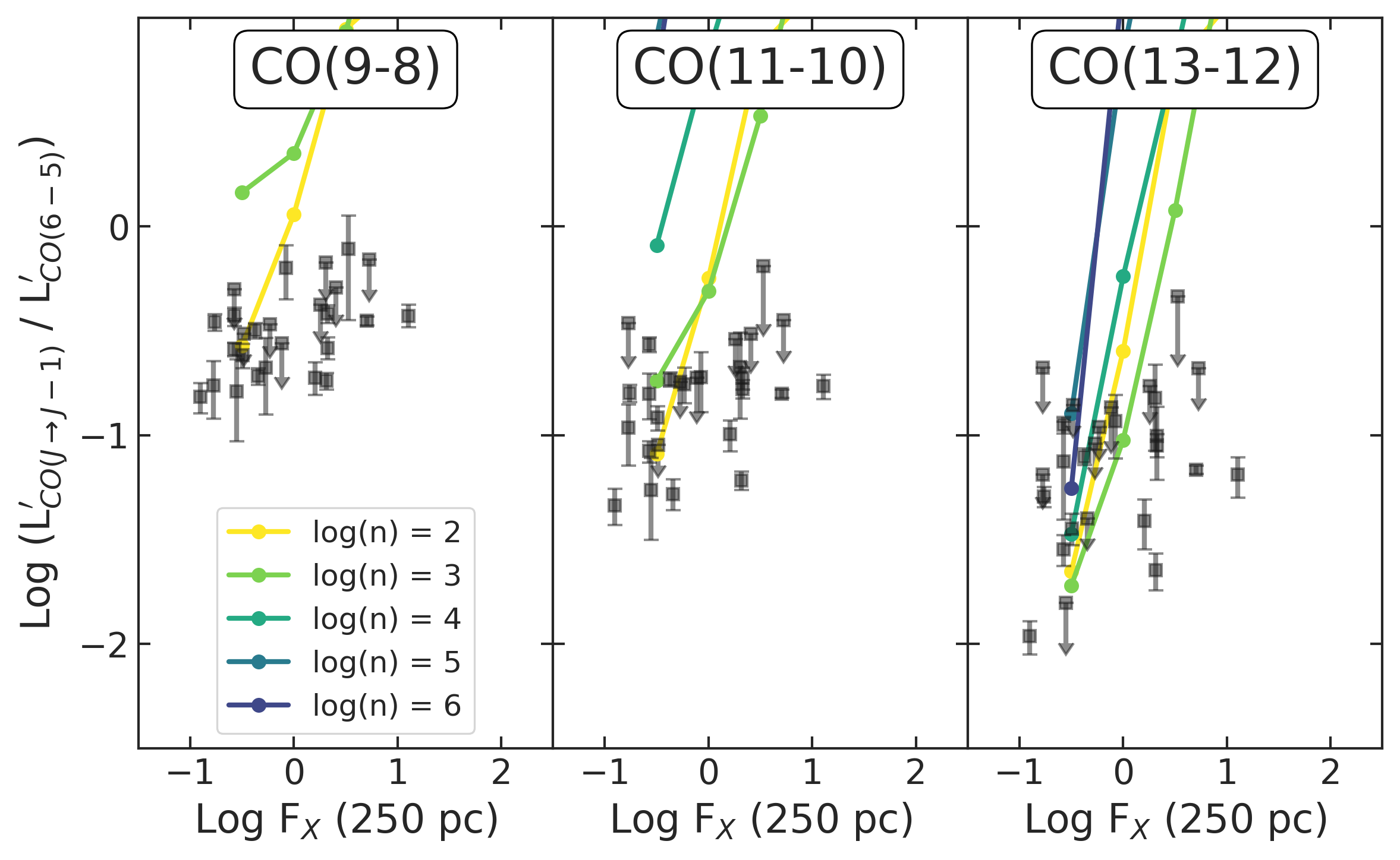
Figure 5: Top-left: $G_{0}$ vs. CO ratio to the nuclear ($r=250$ pc) fraction of CO(1–0). Top-right: $G_{0}$ vs. CO ratio to the CO(6–5) line. Bottom-left: $F_{\rm X}$ vs. CO ratio to the nuclear ($r=250$ pc) fraction of CO(1–0). Bottom-right: $F_{\rm X}$ vs. CO ratio to the CO(6–5) line. In all the plots, the points are the same of Figure 3 and Figure 4. Both $G_{0}$ and $F_{X}$ are measured at $r=250$ pc. The coloured overplotted lines are from numerical Cloudy models of different gas densities $n$, namely $10^{2}$ (yellow), $10^{3}$ (light green), $10^{4}$ (aqua green), $10^{5}$ (light blue) and $10^{6}$ (dark blue) cm^-3.

Compared to the PDR results shown in Figure 3, for the XDR we find lower regression slopes: $0.1-0.5$ for the CO(1–0) ratios, $0-0.2$ for the CO(6–5) ratios. We interpret this as a sign that neither $F_{\text{X}}$ is the dominant driver of these CO lines. Given the physics of high-$J$ CO line emission, which originate from warm molecular gas, the X-ray influence was expected to show up in the correlation with the line ratios, especially those with respect to the low-$J$ CO lines, as found by many theoretical (Maloney et al., 1996; Meijerink & Spaans, 2005; Meijerink et al., 2007) and observational (van der Werf et al., 2010; Pozzi et al., 2017; Mingozzi et al., 2018) works on XDR. A plausible explanation is that at $r=250$ pc we are still outside of the actual AGN sphere of influence of the molecular gas: several studies on Seyfert galaxies (Davies et al., 2007; Kawakatu & Wada, 2008; Esquej et al., 2014; Motter et al., 2021) indeed place it within the central $r=100$ pc. At larger radii, we cannot isolate the contribution of X-rays due to dilution with stellar FUV photons. Unfortunately, our Herschel CO observations have limited spatial resolution to reach such a nuclear region, and ALMA is still limited to the low/mid-$J$ lines, at least in the local Universe.

5.3 Comparison with models

We use predictions from numerical models presented in Vallini et al. (2019) to interpret the observations, in order to shed light on the dominant heating source in the molecular ISM of our galaxies. For this purpose, we use Cloudy (Ferland et al., 2017) to compute the CO line intensities emerging from a 1-D gas slab of density $n$, illuminated by either FUV flux $G_{0}$ (PDR models) or a X-ray flux $F_{\rm X}$ (XDR models). The results of these simulations mainly apply for a single cloud, while we are dealing with entire galaxies (or at least their inner regions); it is therefore especially convenient to study the effect on the line ratios, rather than line fluxes or luminosities, assuming that both numerators and denominators originate from the same area.

The gas density $n$ is a fundamental missing quantity in our analysis of PDR and XDR. We do have some indications of its possible value: from the X-ray-derived column density, we estimated mean volume densities between $n\approx 10^{1-3}$ cm^-3 (Section 3.1) within $r=250$ pc. It is however possible, from the comparison of observed CO ratios with PDR and XDR Cloudy models outputs, to estimate the density of the dissociation region from which the observed CO lines originate.

In the four panels of Figure 5, we examine the PDR and XDR predictions, respectively made with $\log G_{0}=[2,3,4,5]$ and $\log(F_{\text{X}}/(\text{erg s}^{-1}\text{cm}^{-2}))=[-0.5,0,0.5,1,1.5,2,2.5]$, with modelled gas density $\log(n/\text{cm}^{-3})=[2,3,4,5]$. Again we explore the CO line ratio to CO(1–0) and CO(6–5), using the same three mid-/high-$J$ lines as in Figure 3 and 4. The same plots with all the CO lines can be found at the end of Appendix A. The modelled points are plotted in the panels of Figure 5, colour coded with $n$.

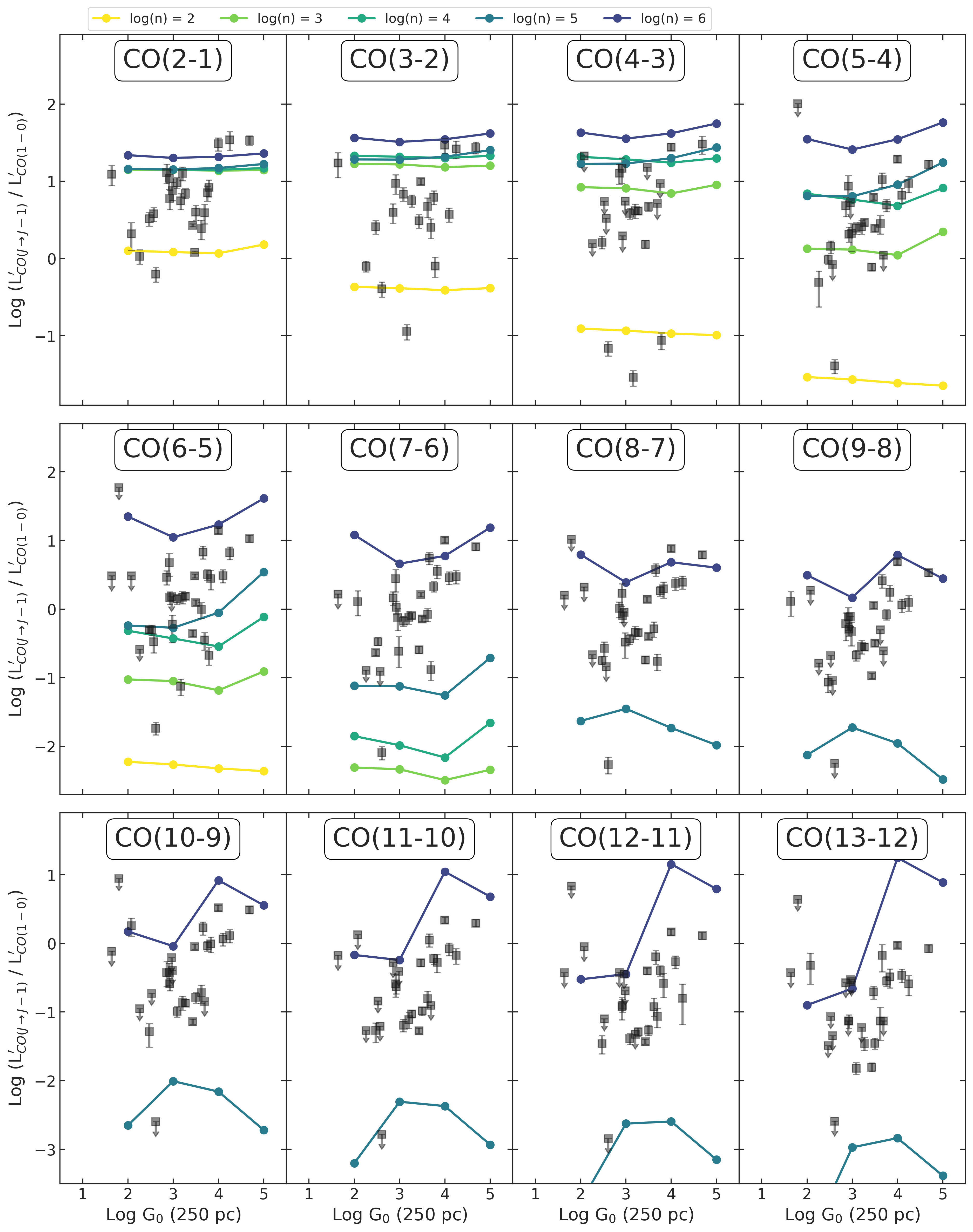
Figure 10: CO line ratios, with respect to the CO(1–0) line, vs. $G_{0}$. The $x$-axis is the Habing field $G_{0}$ (for $r=250$ pc). The $y$-axis is the luminosity ratio $L^{\prime}_{\text{CO}(J\rightarrow J-1)}/L^{\prime}_{\text{CO}(1\rightarrow 0)}$ to the nuclear ($r=250$ pc) fraction of CO(1–0). The luminosities $L^{\prime}$ are in units of K km s^-1 pc^-2, and $J$ is indicated on the top of each panel. Squares with downward arrow indicate less than $3\sigma$ detections in the higher-$J$ line (i.e. censored data). The colored overplotted lines are Cloudy numerical models at different gas densities, namely $10^{2}$ (yellow), $10^{3}$ (light green), $10^{4}$ (dark green), $10^{5}$ (blue) and $10^{6}$ (purple) cm^-3.

In the PDR case, almost all our galaxies are reproduced considering densities in the $n=10^{5-6}$ cm^-3 range, except for the line ratios up to CO(6–5), as can be seen on the leftmost panel ($L^{\prime}_{CO(6-5)}/L^{\prime}_{CO(1-0)}$) of Figure 5, and even better in the first lines of Figure 10 and 11. Previous PDR studies did not find such high densities. The only exception is Mrk 231, for which van der Werf et al. (2010) obtained a warm PDR component with $G_{0}=10^{3.5}$ and $n=10^{5}$ cm^-3; however, such a high density is necessary to reproduce the mid-$J$ emission, while a colder PDR component, with $n=10^{3.5}$ cm^-3, reproduces the low-$J$ emission and accounts for most of the gas volume. Díaz-Santos et al. (2017) observed instead that on average, and on the scale of the whole galaxy, local (U)LIRGs start from a minimum $G_{0}/n\sim 10^{-1}$, and that this ratio increases with the IR luminosity surface density; this would place an upper limit to the gas density at a fixed $G_{0}$. In the top panels of Figure 5, instead, our galaxies, for $J_{\text{upp}}\geq 8$, lie in the range $\log(G_{0}/n)=[-4,-1]$, given the modelled gas densities. It is necessary for PDR models to have high densities to produce bright mid-$J$ transitions (Vallini et al., 2018), and it is known (e.g. McKee & Ostriker, 2007) that such densities are typical of clumps and cores in single star-forming molecular clouds (as shown by Joblin et al., 2018, in e.g. the Orion Bar). Nonetheless, it is unlikely that the central 500 pc of galaxies have an average gas density of $10^{5-6}$ cm^-3, so we expect these high-density regions to have a very low volume filling factor.

In the XDR case, on the contrary, the models with low density ($n\approx 10^{2-3}$ cm^-3) can reproduce the observed CO line ratios, at least in the regions of the parameters space where the lines with such densities are clearly separable from the others. This result is in line with the densities ($n\approx 10^{1-3}$ cm^-3) calculated from the X-ray-derived $N_{\rm H}$, and from what we expect from the available XDR studies for local (U)LIRGs (van der Werf et al., 2010; Pozzi et al., 2017; Mingozzi et al., 2018). From Figure 5 it is clear that the observed high-$J$ line ratios (especially $J_{\text{upp}}\geq 12$) can be reproduced by either a high $F_{X}$ or a high $n$, a degeneracy also found in the semi-analytic model by Vallini et al. (2019). However, both our high-$J$ line ratios and our calculated $F_{\text{X}}$ are lowered by the nuclear radius we are using ($r=250$ pc), so a detailed numerical modelling at different distances from the AGN is needed to really see the impact of XDR on the molecular emission.

We note here that stars and AGN can also affect the heating of molecular gas through outflows/winds, resulting in shock-heated regions (Kazandjian et al., 2012; Aalto et al., 2012; García-Burillo et al., 2014) where the brightness of high-J CO lines is enhanced too. Disentangling the contribution of shock heating from that produced in XDRs is a challenging task (Hollenbach & McKee, 1989; Meijerink et al., 2013; Mingozzi et al., 2018). However, the study of mechanical heating is beyond the scope of this paper.

6 Conclusions

In this paper, we investigate the relative impact of star formation and AGN activity on the CO rotational line emission. In this respect, we collect multiwavelength (mm, IR and X-ray) data for a sample of 35 local active galaxies. The sources are selected with a well-sampled CO SLED (from $J=1-0$ to $J=13-12$) and intrinsic $L_{X}\geq 10^{42}$ erg s^-1 in the 2–10 keV range. From the multiband data we derive, in a homogeneous way, key integrated physical quantities, as the molecular gas mass ($M_{\text{mol}}$), the star formation FUV flux ($G_{0}$) and the AGN X-ray flux, $F_{\rm X}$. Moreover, by analysing the ALMA images of the highest available CO emission, we estimate the emitting area of mid-$J$/high-$J$ CO lines, finding it concentrated within $r=250$ pc from the center. To determine whether AGN activity influences the molecular gas in its vicinity, we measure FUV and X-ray radiation, producing PDR and XDR, respectively, from the observational data in a self-consistent way. The FUV flux is parametrized in terms of $G_{0}$, gauged from the 70 $\mu$m, spatially resolved, dust emission, the $F_{X}$ is calculated from the intrinsic $L_{X}$. Our main results can be summarized as follows:

1. On the kpc-scale of the whole galaxy (namely within a median $r_{\text{CO}}=3.1^{+2.1}_{-1.5}$ kpc) we do not find measurable evidence for the AGN influence on the star formation. Our sample results well mixed with other samples of non-active galaxies on the Schmidt-Kennicutt ($\Sigma_{\text{mol}}$ vs. $\Sigma_{\text{SFR}}$) plane. If we use a Milky Way CO-to-H₂ conversion factor $\alpha_{\text{CO}}=4.3$ M_⊙ (K km s^-1 pc^-2)^-1, we find a median $\log(M_{\text{mol}}/M_{\odot})=9.9^{+0.3}_{-0.8}$ for our sample, and a median depletion time $\log(\tau_{\text{depl}}/\text{yr})=8.9^{+0.4}_{-0.6}$.

2. We measure within $r=250$ pc the irradiation of PDR and XDR by deriving $G_{0}$ and $F_{X}$, finding $\log G_{0}=3.1^{+0.7}_{-0.8}$ and $\log(F_{\text{X}}/(\text{erg s}^{-1}\text{cm}^{-2}))=-0.1_{-0.5}^{+0.8}$ for our sample. These values are comparable with the literature for local active galaxies, for both observational and theoretical works.

3. We find weak correlations between $G_{0}$, $F_{\text{X}}$ and two different CO line ratios, namely to the nuclear ($r=250$ pc) fraction of CO(1–0) and to CO(6–5). Therefore, neither $G_{0}$ nor $F_{\text{X}}$ alone can produce the observed molecular emission.

4. From the comparison of CO emission and observed $G_{0}$ with grids of PDR numerical models, we can conclude that PDR emission can reproduce observed high-$J$ line ratios only assuming unlikely extreme gas densities ($n>10^{5}$ cm^-3), while it is more efficient at moderate densities ($n\sim 10^{3-4}$ cm^-3) up to CO(6–5).

5. From the comparison between XDR observations and models, we find that $F_{\text{X}}$ can reproduce the observed low-/mid-$J$ CO line ratios only at low densities ($n\sim 10^{2}$ cm^-3), similar to those estimated from X-ray column densities ($n\sim 10^{1-3}$ cm^-3). At high-$J$ we find increasing (with $J$) degeneracy between $F_{\text{X}}$ and $n$, so we can not find a typical gas density for our sample. This is probably an indication that the nuclear scale at which we are considering the XDR is still too large to see a strong AGN effect on the CO SLED.

From our analysis, we conclude that, on scales of $\approx$250 pc from the galaxy center, a mix of PDR and XDR is necessary to explain the observed CO emission, since neither of them is the dominant mechanism. The use of the CO SLED to disentangle the contribution of FUV and/or X-rays photons to the molecular gas heating in local galaxies is currently limited by the low spatial resolution at the high-$J$ frequencies ($\sim 17$ arcsec for CO(13–12) with Herschel/PACS). Conversely, high-$z$ galaxies have their high-$J$ CO emission redshifted into the observation bands of ALMA and NOEMA, which are able to reach sub-arcsec resolution. These extreme CO lines have been observed and modelled already by several works (Gallerani et al., 2014; Carniani et al., 2019; Pensabene et al., 2021). It would be therefore interesting to extend the analysis performed in this paper on a high-redshift sample of active galaxies with spatially resolved CO emission, and assess possible differences with local AGN.

Data Availability

The data underlying this article were accessed from the ALMA Archive (https://almascience.eso.org/asax/), from the JVO portal (http://jvo.nao.ac.jp/portal) operated by the NAOJ, and the NASA/IPAC Infrared Science Archive (specifically https://irsa.ipac.caltech.edu/data/Herschel/HHLI/overview.html), which is funded by the National Aeronautics and Space Administration and operated by the California Institute of Technology The derived data generated in this research will be shared on reasonable request to the corresponding author.

Appendix A CO line ratios

In this section we show the CO luminosity ratios, both with denominators the CO(1–0) and the CO(6–5) luminosity. The CO(1–0) luminosities have been corrected to take into account only the emission up to $r=250$ pc from the center of the galaxies (with Equation 1). Firstly we plot the luminosity ratios against the FUV flux $G_{0}$ and the X-ray flux $F_{\text{X}}$, fitting the points with a regression line, respectively as in Figures 3 and 4. The details can be found in Sections 5.1 and 5.2. Secondly, we plot the same points but with the Cloudy models at different gas densities superimposed, as in Figure 5, and as explained in detail in Section 5.3.

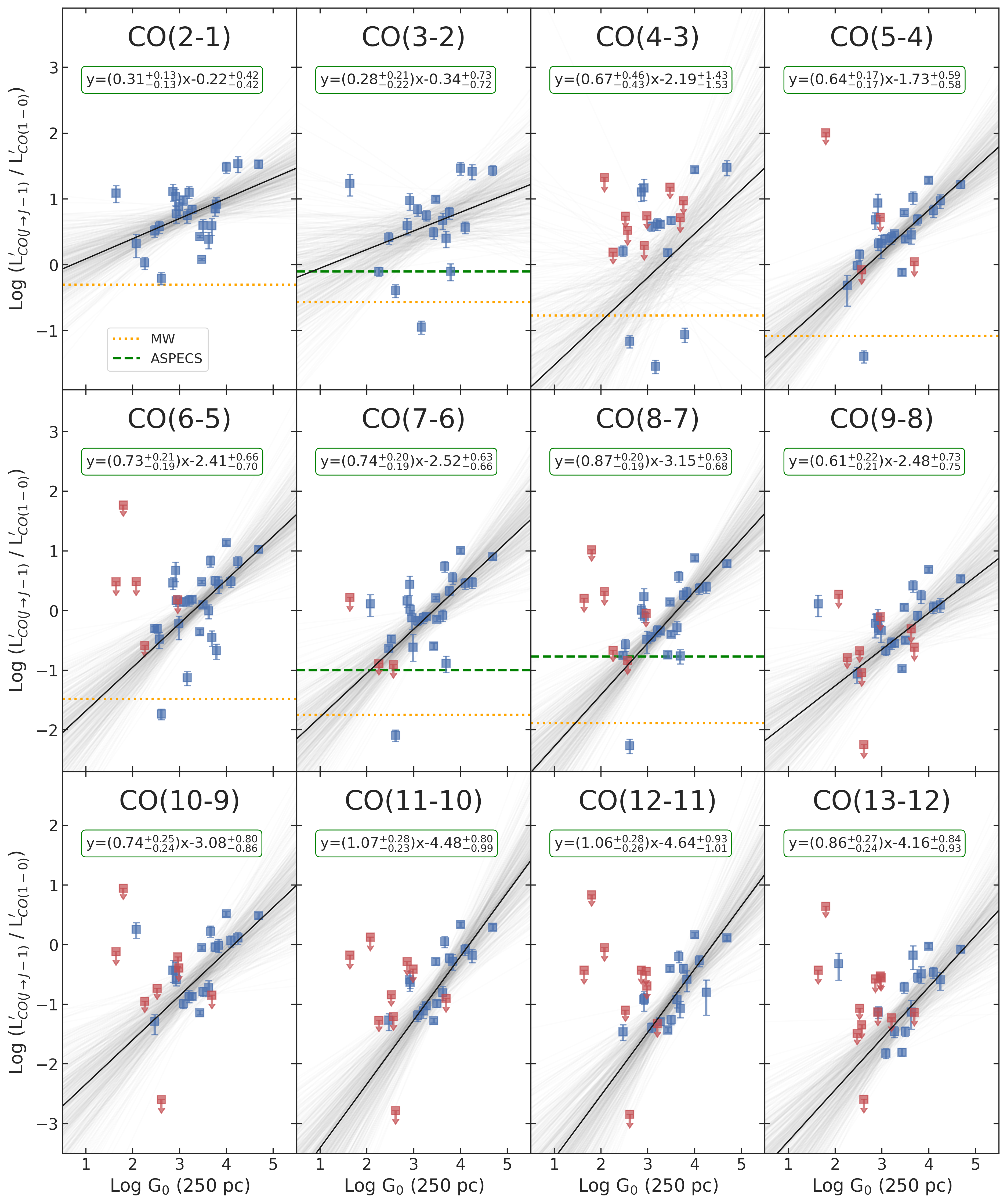
Figure 6: CO line ratios, with respect to the CO(1–0) line, vs. $G_{0}$. The $x$-axis is the Habing field $G_{0}$ (for $r=250$ pc). The $y$-axis is the luminosity ratio $L^{\prime}_{\text{CO}(J\rightarrow J-1)}/L^{\prime}_{\text{CO}(1\rightarrow 0)}$ to the nuclear ($r=250$ pc) fraction of CO(1–0). The luminosities $L^{\prime}$ are in units of K km s^-1 pc^-2, and $J$ is indicated on the top of each panel. Blue squares indicate $3\sigma$ detections in both lines; red squares with downward arrow indicate less than $3\sigma$ in the higher-$J$ line (i.e. censored data). The lines are regression fits to the observed data: solid black line is the median Linmix regression, thin shaded green lines show fits drawn from the posterior distribution of Linmix regression. When available, the Milky Way (dotted orange line, data from Fixsen et al. 1999) and the ASPECS AGN (green dashed line, data from Boogaard et al. 2020) CO ratios are also shown.

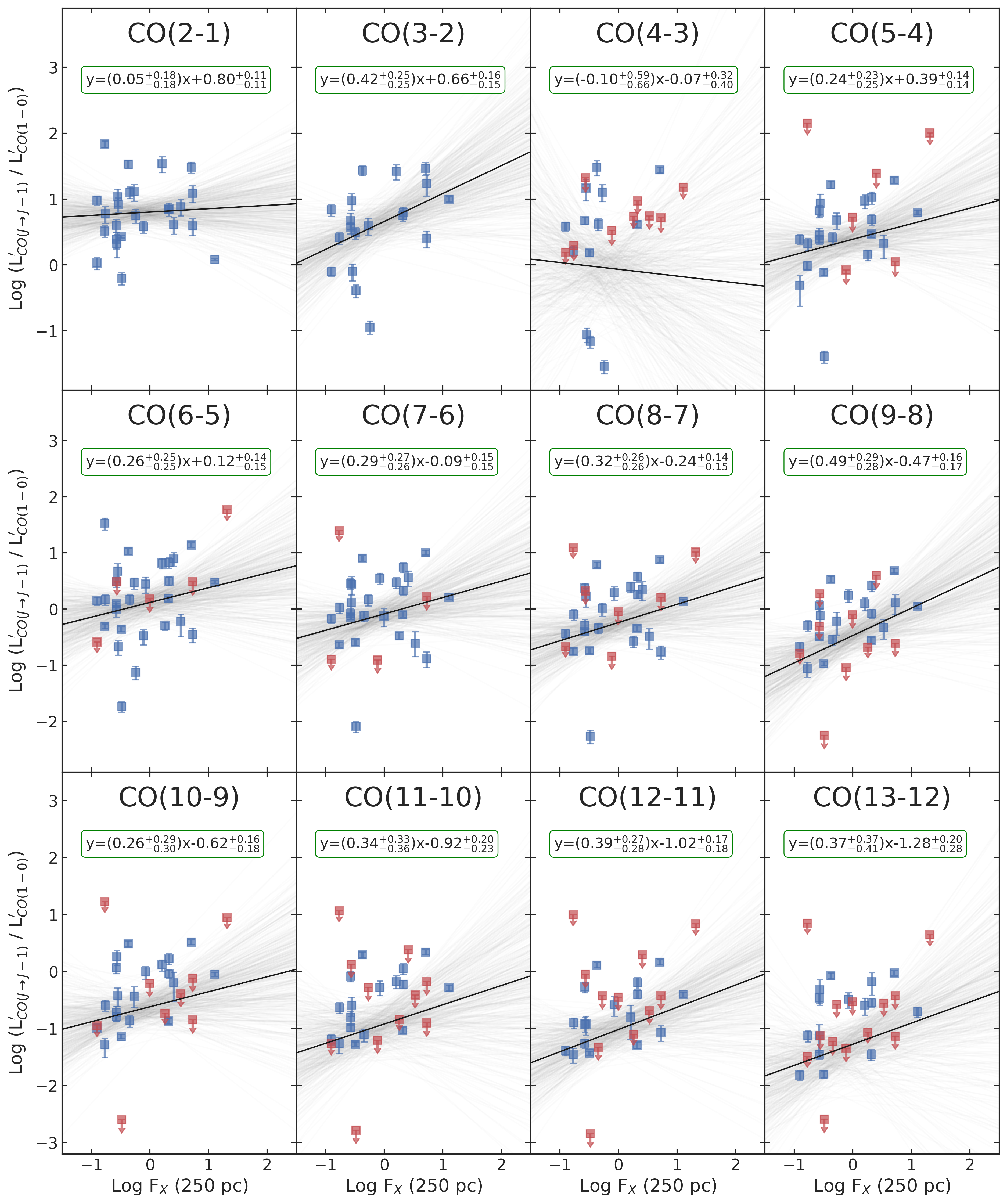
Figure 8: CO line ratios, with respect to the CO(1–0) line, vs. $F_{X}$. The $x$-axis is $F_{X}$ (for $r=250$ pc), in units of erg s^-1 cm^-2. The $y$-axis is the luminosity ratio $L^{\prime}_{\text{CO}(J\rightarrow J-1)}/L^{\prime}_{\text{CO}(1\rightarrow 0)}$ to the nuclear ($r=250$ pc) fraction of CO(1–0). Data points and lines are described in Figure 6.

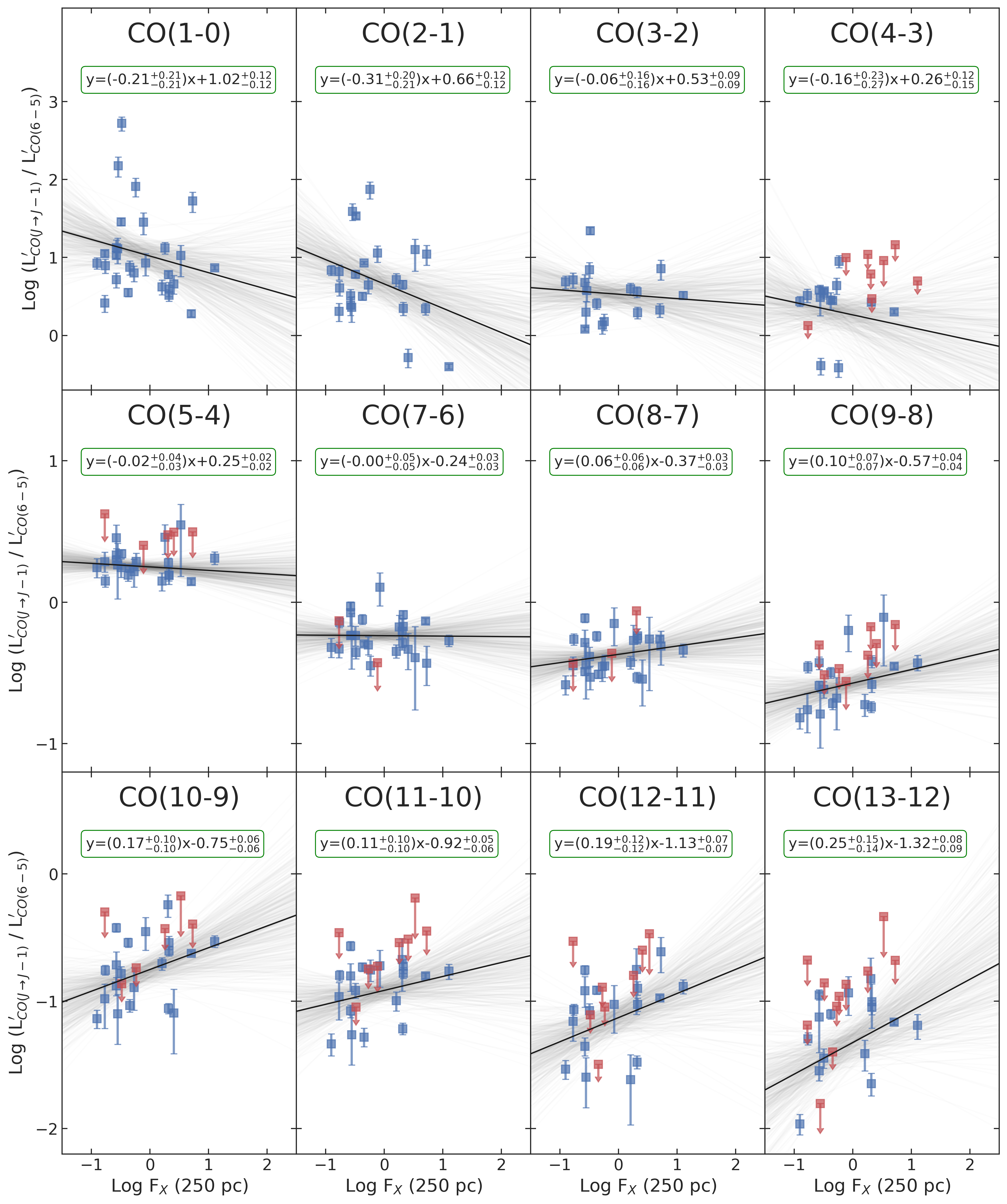
Figure 9: CO line ratios, with respect to the CO(6–5) line, vs. $F_{X}$. The $x$-axis is $F_{X}$ (for $r=250$ pc), in units of erg s^-1 cm^-2. The $y$-axis is the luminosity ratio $L^{\prime}_{\text{CO}(J\rightarrow J-1)}/L^{\prime}_{\text{CO}(6\rightarrow 5)}$ to the CO(6–5) line. Data points and lines are described in Figure 6.

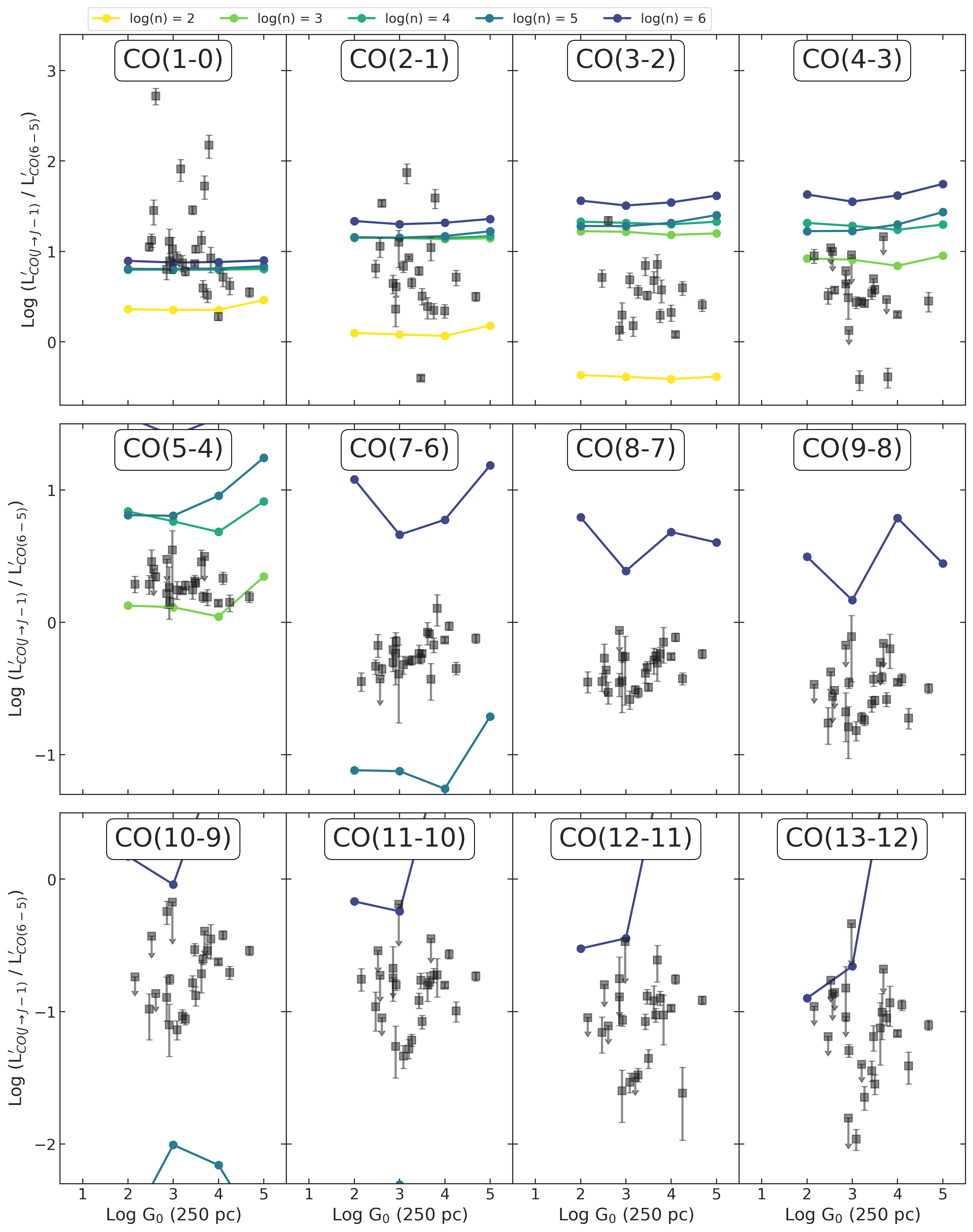
Figure 11: CO line ratios, with respect to the CO(6–5) line, vs. $G_{0}$. The $x$-axis is the Habing field $G_{0}$ (for $r=250$ pc). The $y$-axis is the luminosity ratio $L^{\prime}_{\text{CO}(J\rightarrow J-1)}/L^{\prime}_{\text{CO}(6\rightarrow 5)}$ to the CO(6–5) line. Data points and lines are described in Figure 10.

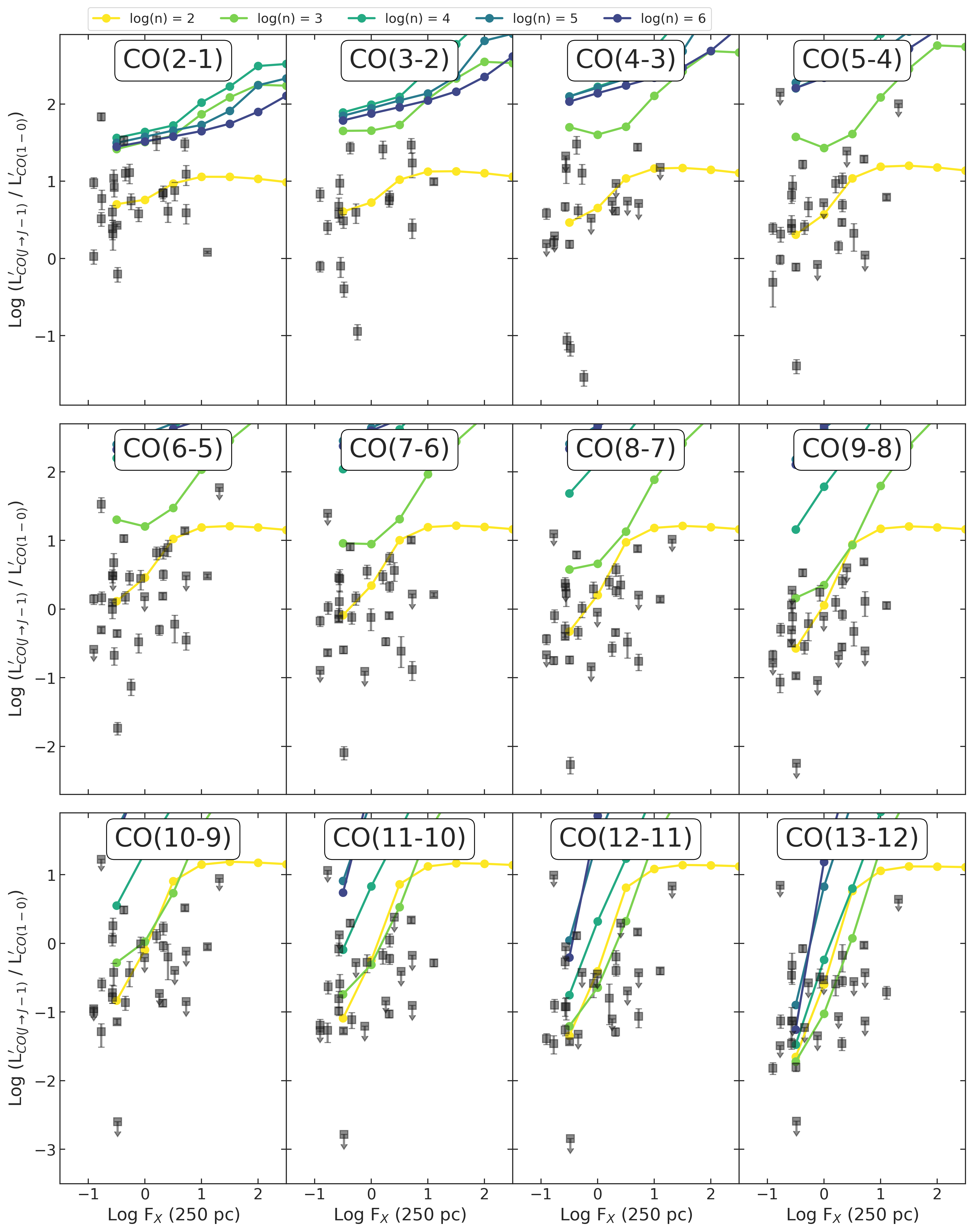
Figure 12: CO line ratios, with respect to the CO(1–0) line, vs. $F_{X}$. The $x$-axis is $F_{X}$ (for $r=250$ pc), in units of erg s^-1 cm^-2. The $y$-axis is the luminosity ratio $L^{\prime}_{\text{CO}(J\rightarrow J-1)}/L^{\prime}_{\text{CO}(1\rightarrow 0)}$ to the nuclear ($r=250$ pc) fraction of CO(1–0). Data points and lines are described in Figure 10.

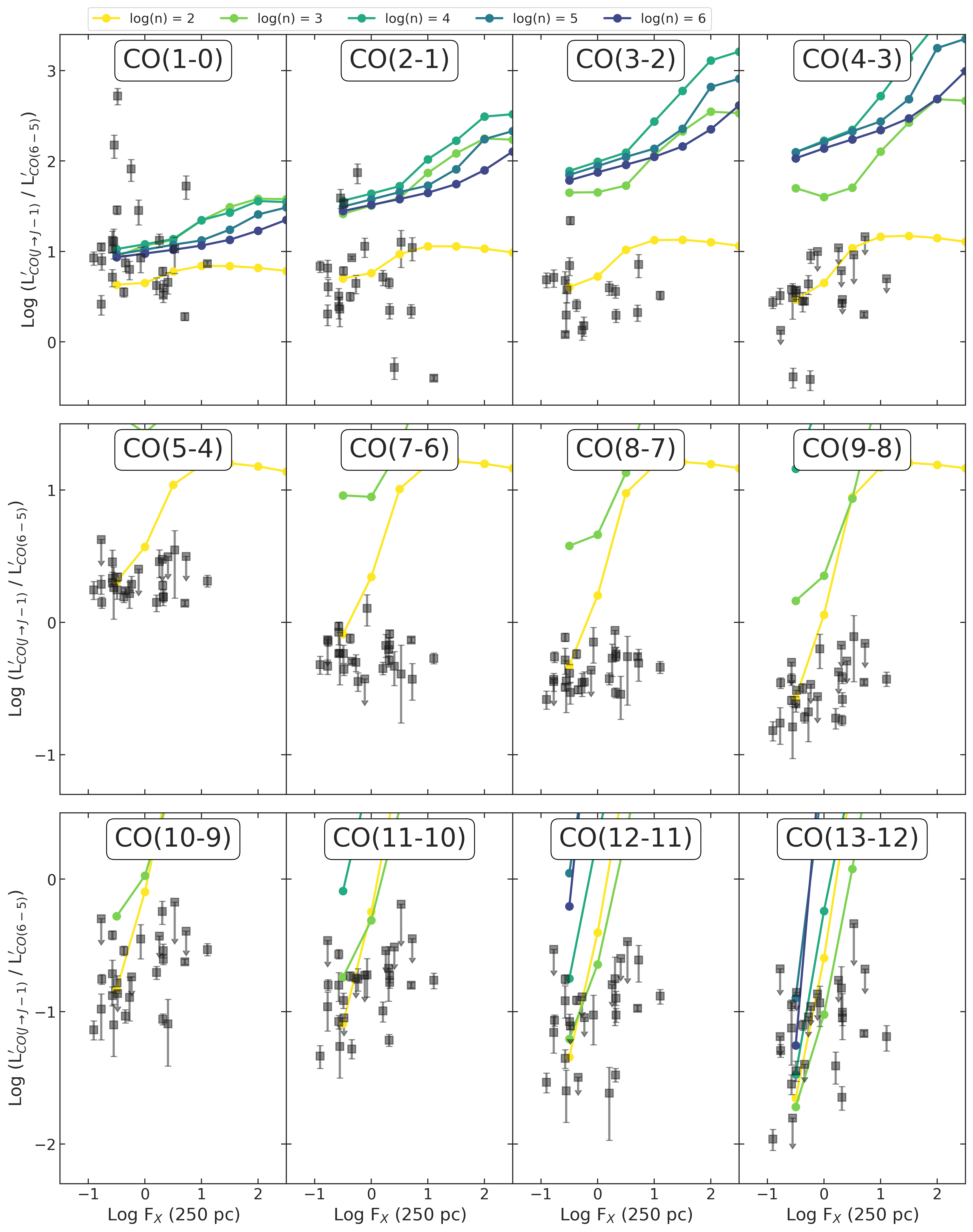
Figure 13: CO line ratios, with respect to the CO(6–5) line, vs. $F_{X}$. The $x$-axis is $F_{X}$ (for $r=250$ pc), in units of erg s^-1 cm^-2. The $y$-axis is the luminosity ratio $L^{\prime}_{\text{CO}(J\rightarrow J-1)}/L^{\prime}_{\text{CO}(6\rightarrow 5)}$ to the CO(6–5) line. Data points and lines are described in Figure 10.

Appendix B CO(6–5) atlas

In this section we present the rest (in addition to Figure 1) of the images of CO(6–5) emission for our sample galaxies. All the CO(6–5) data cubes are from the ALMA Archive, already calibrated, cleaned, and when available, primary-beam corrected. Using CASA 5.6 (McMullin et al., 2007), we produce the moment 0 map from the data cubes with the task immoments. We then plot the ALMA CO(6–5) contours over the optical image of the galaxy.

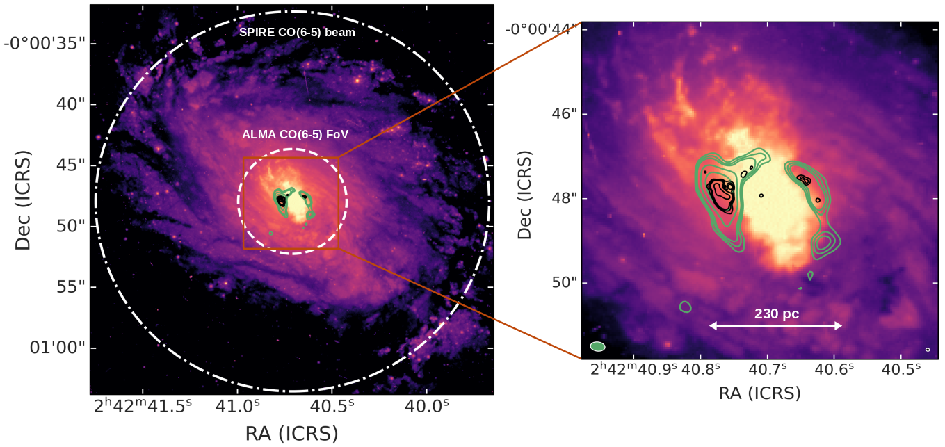
Figure 14: Left panel: HST WFPC2 F606W image of NGC 1068 (from Malkan et al. 1998) with superimposed the contours of two ALMA CO(6–5) observations, in green at the resolution of 250 mas (project 2011.0.00083.S, PI: García-Burillo), in black of 90 mas (project 2013.1.00014.S, PI: Elitzur). Both the contours are at the respective (3, 4, 5, 10, 20) $\times\,\sigma$, where $\sigma=6.2$ Jy beam^-1 km s^-1 for the green lines and $\sigma=1.1$ Jy beam^-1 km s^-1 for the black lines. The inner white dashed circle indicates the FoV of both ALMA observations, with a radius of 4$\aas@@fstack{\prime\prime}$3 ($\sim$340 pc), while the outer dash-dotted circle represents the Herschel/SPIRE-FTS beam FWHM for CO(6–5) observations, with a 15$\aas@@fstack{\prime\prime}$6 radius. Right panel: zoom of the inner 670 pc. Restored ALMA beams of the 250 and 90 mas images are shown as ellipses with white edges, at the bottom left (with the green area) and right (with the black area), respectively. The 250 mas ALMA image has not been primary-beam corrected.

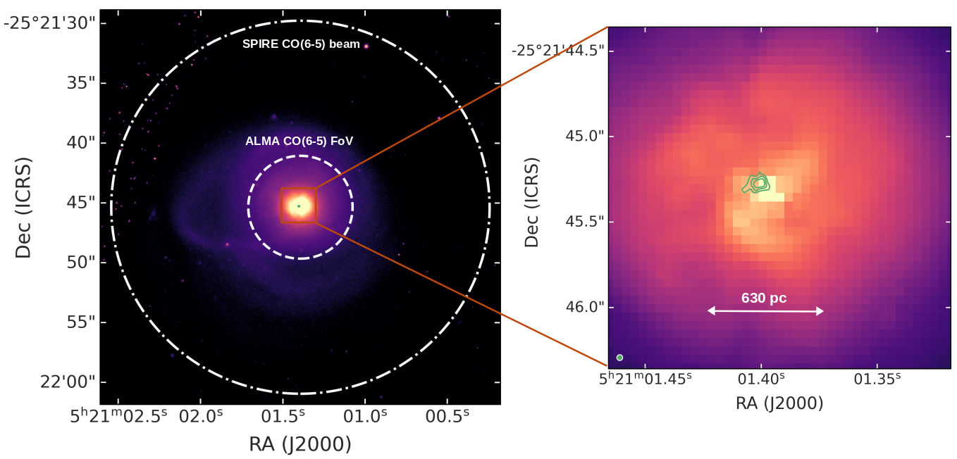
Figure 15: Left panel: HST ACS F814W image of IRAS F05189–2524 (from Evans 2005), with superimposed, in green, the contours of ALMA CO(6–5) moment 0 at the resolution of 40 mas (project 2016.1.01223.S, PI: Baba). The contours are drawn at (3, 4, 5, 10, 20) $\times\,\sigma$, where $\sigma=0.55$ Jy beam^-1 km s^-1. The inner white dashed circle indicates the FoV of both ALMA observations, with a radius of 4$\aas@@fstack{\prime\prime}$3 ($\sim$3.6 kpc), while the outer dash-dotted circle represents the Herschel/SPIRE-FTS beam FWHM for CO(6–5) observations, with a 15$\aas@@fstack{\prime\prime}$6 radius. Right panel: zoom of the inner 1.7 kpc. The restored ALMA beam is shown as a green ellipse with white edges at the bottom left.

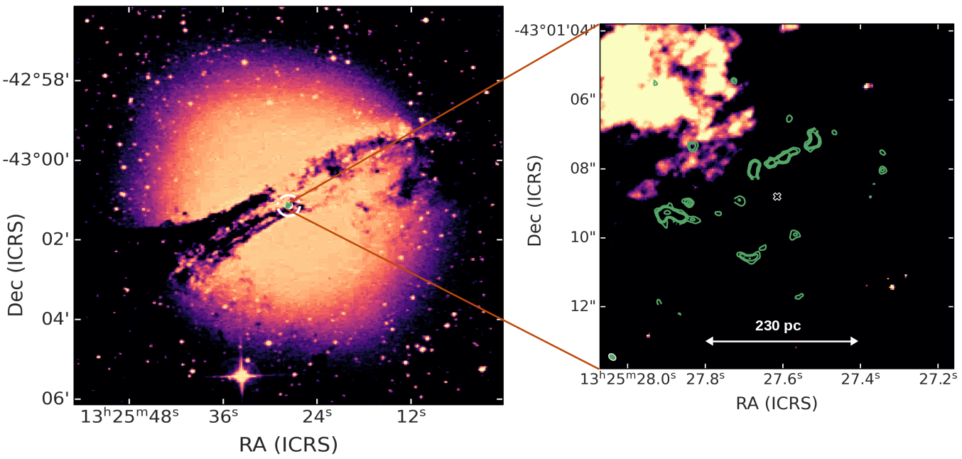
Figure 16: Left panel: DSS-2 B-band image of NGC 5128. The inner white dashed circle indicates the FoV of both ALMA observations, with a radius of 4$\aas@@fstack{\prime\prime}$3 ($\sim$160 pc), while the outer dash-dotted circle represents the Herschel/SPIRE-FTS beam FWHM for CO(6–5) observations, with a 15$\aas@@fstack{\prime\prime}$6 radius. Right panel: zoom of the inner 380 pc, with HST WFPC2 F555W image of NGC 5128 (from Marconi et al. 2000) in the background, with superimposed, in green, the contours of ALMA CO(6–5) moment 0 at the resolution of 170 mas (project 2012.1.00225.S, PI: Espada). The contours are drawn at (3, 4, 5, 10, 20) $\times\,\sigma$, where $\sigma=0.42$ Jy beam^-1 km s^-1. The restored ALMA beam is shown as a green ellipse with white edges at the bottom left. A "X" marker, black with white edges, indicates the center of the galaxy.

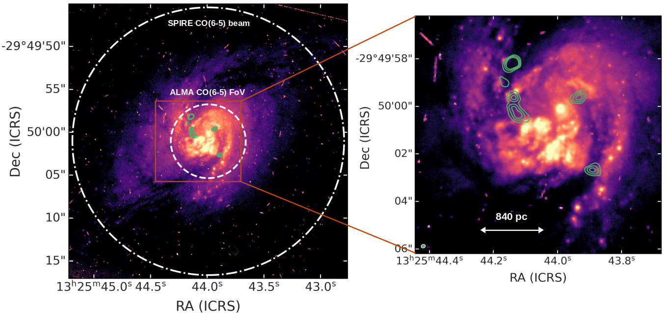
Figure 17: Left panel: HST WFPC2 F606W image of NGC 5135 (from Malkan et al. 1998), with superimposed, in green, the contours of ALMA CO(6–5) moment 0 at the resolution of 170 mas (project 2013.1.00524.S, PI: Lu). The contours are drawn at (3, 4, 5, 10, 20) $\times\,\sigma$, where $\sigma=1.2$ Jy beam^-1 km s^-1. The inner white dashed circle indicates the FoV of both ALMA observations, with a radius of 4$\aas@@fstack{\prime\prime}$3 ($\sim$1.2 kpc), while the outer dash-dotted circle represents the Herschel/SPIRE-FTS beam FWHM for CO(6–5) observations, with a 15$\aas@@fstack{\prime\prime}$6 radius. Right panel: zoom of the inner 2.5 kpc. The restored ALMA beam is shown as a green ellipse with white edges at the bottom left.

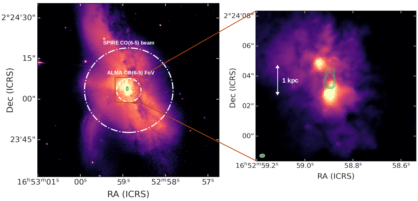
Figure 18: Left panel: HST WFPC2 F814W image of NGC 6240 (from Gerssen et al. 2004), with superimposed, in green, the contours of ALMA CO(6–5) moment 0 at the resolution of 250 mas (project 2015.1.00658.S, PI: Rangwala). The contours are drawn at (3, 4, 5, 10, 20) $\times\,\sigma$, where $\sigma=29$ Jy beam^-1 km s^-1. The inner white dashed circle indicates the FoV of both ALMA observations, with a radius of 4$\aas@@fstack{\prime\prime}$3 ($\sim$2.1 kpc), while the outer dash-dotted circle represents the Herschel/SPIRE-FTS beam FWHM for CO(6–5) observations, with a 15$\aas@@fstack{\prime\prime}$6 radius. Right panel: zoom of the inner 4.5 kpc. The restored ALMA beam is shown as a green ellipse with white edges at the bottom left.

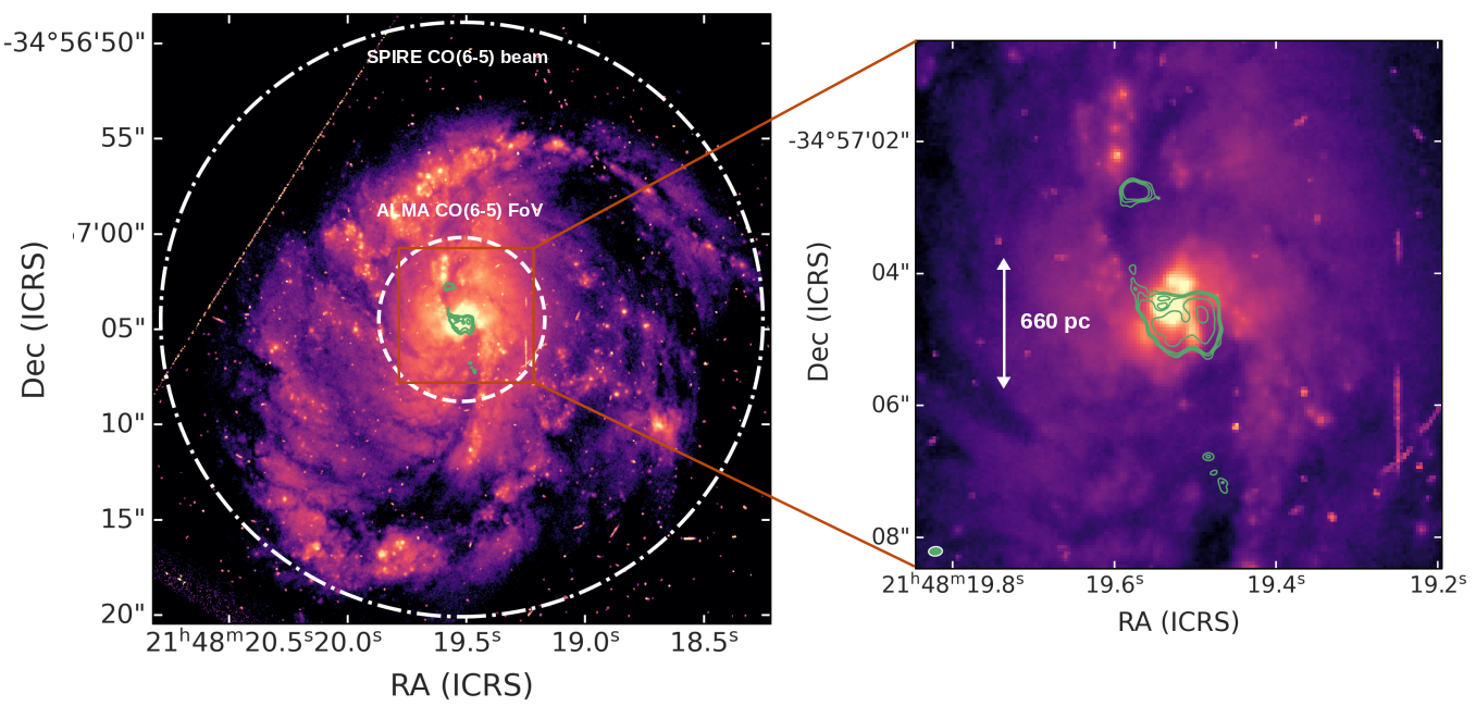
Figure 19: Left panel: HST WFPC2 F606W image of IRAS F05189–2524 (from Malkan et al. 1998), with superimposed, in green, the contours of ALMA CO(6–5) moment 0 at the resolution of 180 mas (project 2013.1.00524.S, PI: Lu). The contours are drawn at (3, 4, 5, 10, 20) $\times\,\sigma$, where $\sigma=1.5$ Jy beam^-1 km s^-1. The inner white dashed circle indicates the FoV of both ALMA observations, with a radius of 4$\aas@@fstack{\prime\prime}$3 ($\sim$1.4 kpc), while the outer dash-dotted circle represents the Herschel/SPIRE-FTS beam FWHM for CO(6–5) observations, with a 15$\aas@@fstack{\prime\prime}$6 radius. Right panel: zoom of the inner 2.3 kpc. The restored ALMA beam is shown as a green ellipse with white edges at the bottom left. This ALMA image has not been primary-beam corrected.

References

- Aalto et al. (1995) Aalto S., Booth R. S., Black J. H., Johansson L. E. B., 1995, A&A, 300, 369
- Aalto et al. (2012) Aalto S., Garcia-Burillo S., Muller S., Winters J. M., van der Werf P., Henkel C., Costagliola F., Neri R., 2012, A&A, 537, A44
- Albrecht et al. (2007) Albrecht M., Krügel E., Chini R., 2007, A&A, 462, 575
- Alloin et al. (1992) Alloin D., Barvainis R., Gordon M. A., Antonucci R. R. J., 1992, A&A, 265, 429
- Alonso-Herrero et al. (2011) Alonso-Herrero A., et al., 2011, ApJ, 736, 82
- Alonso-Herrero et al. (2012) Alonso-Herrero A., Pereira-Santaella M., Rieke G. H., Rigopoulou D., 2012, ApJ, 744, 2
- Astropy Collaboration et al. (2013) Astropy Collaboration et al., 2013, A&A, 558, A33
- Astropy Collaboration et al. (2018) Astropy Collaboration et al., 2018, AJ, 156, 123
- Ballantyne (2008) Ballantyne D. R., 2008, ApJ, 685, 787
- Barthelmy et al. (2005) Barthelmy S. D., et al., 2005, Space Sci. Rev., 120, 143
- Bellocchi et al. (2016) Bellocchi E., Arribas S., Colina L., 2016, A&A, 591, A85
- Bendo et al. (2009) Bendo G. J., Clements D. L., Khan S. A., 2009, MNRAS, 399, L29
- Bianchi et al. (2008) Bianchi S., Chiaberge M., Piconcelli E., Guainazzi M., Matt G., 2008, MNRAS, 386, 105
- Bigiel et al. (2008) Bigiel F., Leroy A., Walter F., Brinks E., de Blok W. J. G., Madore B., Thornley M. D., 2008, AJ, 136, 2846
- Boch & Fernique (2014) Boch T., Fernique P., 2014, in Manset N., Forshay P., eds, Astronomical Society of the Pacific Conference Series Vol. 485, Astronomical Data Analysis Software and Systems XXIII. p. 277
- Bolatto et al. (2013) Bolatto A. D., Wolfire M., Leroy A. K., 2013, ARA&A, 51, 207
- Bonnarel et al. (2000) Bonnarel F., et al., 2000, A&AS, 143, 33
- Boogaard et al. (2020) Boogaard L. A., et al., 2020, ApJ, 902, 109
- Boselli et al. (2014) Boselli A., Cortese L., Boquien M., 2014, A&A, 564, A65
- Bradley et al. (2020) Bradley L., et al., 2020, astropy/photutils: 1.0.0, doi:10.5281/zenodo.4044744, https://doi.org/10.5281/zenodo.4044744
- Brightman & Nandra (2011) Brightman M., Nandra K., 2011, MNRAS, 413, 1206
- Buchner & Bauer (2017) Buchner J., Bauer F. E., 2017, MNRAS, 465, 4348
- Calura et al. (2014) Calura F., Gilli R., Vignali C., Pozzi F., Pipino A., Matteucci F., 2014, MNRAS, 438, 2765
- Calzetti et al. (2010) Calzetti D., et al., 2010, ApJ, 714, 1256
- Carilli & Walter (2013) Carilli C. L., Walter F., 2013, ARA&A, 51, 105
- Carniani et al. (2019) Carniani S., et al., 2019, MNRAS, 489, 3939
- Casasola et al. (2004) Casasola V., Bettoni D., Galletta G., 2004, A&A, 422, 941
- Casasola et al. (2015) Casasola V., Hunt L., Combes F., García-Burillo S., 2015, A&A, 577, A135
- Casasola et al. (2017) Casasola V., et al., 2017, A&A, 605, A18
- Casasola et al. (2020) Casasola V., et al., 2020, A&A, 633, A100
- Comastri (2004) Comastri A., 2004, Compton-Thick AGN: The Dark Side of the X-Ray Background. p. 245, doi:10.1007/978-1-4020-2471-9_8
- Combes et al. (1994) Combes F., Prugniel P., Rampazzo R., Sulentic J. W., 1994, A&A, 281, 725
- Curran et al. (2001) Curran S. J., Polatidis A. G., Aalto S., Booth R. S., 2001, A&A, 368, 824
- D’Amato et al. (2020) D’Amato Q., et al., 2020, A&A, 636, A37
- Dasyra et al. (2016) Dasyra K. M., Combes F., Oosterloo T., Oonk J. B. R., Morganti R., Salomé P., Vlahakis N., 2016, A&A, 595, L7
- Davies et al. (2007) Davies R. I., Müller Sánchez F., Genzel R., Tacconi L. J., Hicks E. K. S., Friedrich S., Sternberg A., 2007, ApJ, 671, 1388
- Decarli et al. (2020) Decarli R., et al., 2020, ApJ, 902, 110
- Díaz-Santos et al. (2017) Díaz-Santos T., et al., 2017, ApJ, 846, 32
- Downes & Solomon (1998) Downes D., Solomon P. M., 1998, ApJ, 507, 615
- Dumas et al. (2010) Dumas G., Schinnerer E., Mundell C. G., 2010, ApJ, 721, 911
- Dunne et al. (2000) Dunne L., Eales S., Edmunds M., Ivison R., Alexander P., Clements D. L., 2000, MNRAS, 315, 115
- Ellison et al. (2019) Ellison S. L., Viswanathan A., Patton D. R., Bottrell C., McConnachie A. W., Gwyn S., Cuillandre J.-C., 2019, MNRAS, 487, 2491
- Espada et al. (2017) Espada D., et al., 2017, ApJ, 843, 136
- Espada et al. (2019) Espada D., et al., 2019, ApJ, 887, 88
- Esquej et al. (2014) Esquej P., et al., 2014, ApJ, 780, 86
- Evans (2005) Evans A., 2005, An ACS Survey of a Complete Sample of Luminous Infrared Galaxies in the Local Universe, HST Proposal
- Evans et al. (2005) Evans A. S., Mazzarella J. M., Surace J. A., Frayer D. T., Iwasawa K., Sanders D. B., 2005, ApJS, 159, 197
- Farrah et al. (2013) Farrah D., et al., 2013, ApJ, 776, 38
- Feltre et al. (2012) Feltre A., Hatziminaoglou E., Fritz J., Franceschini A., 2012, MNRAS, 426, 120
- Ferland et al. (2017) Ferland G. J., et al., 2017, Rev. Mex. Astron. Astrofis., 53, 385
- Fixsen et al. (1999) Fixsen D. J., Bennett C. L., Mather J. C., 1999, ApJ, 526, 207
- Flower & Pineau Des Forêts (2010) Flower D. R., Pineau Des Forêts G., 2010, MNRAS, 406, 1745
- Gallerani et al. (2014) Gallerani S., Ferrara A., Neri R., Maiolino R., 2014, MNRAS, 445, 2848
- Galliano et al. (2003) Galliano E., Alloin D., Granato G. L., Villar-Martín M., 2003, A&A, 412, 615
- Gao & Solomon (1999) Gao Y., Solomon P. M., 1999, ApJ, 512, L99
- Gao & Solomon (2004) Gao Y., Solomon P. M., 2004, ApJS, 152, 63
- García-Burillo et al. (2003) García-Burillo S., et al., 2003, A&A, 407, 485
- García-Burillo et al. (2014) García-Burillo S., et al., 2014, A&A, 567, A125
- Gehrels et al. (2004) Gehrels N., et al., 2004, ApJ, 611, 1005
- Gerssen et al. (2004) Gerssen J., van der Marel R. P., Axon D., Mihos J. C., Hernquist L., Barnes J. E., 2004, AJ, 127, 75
- Golombek et al. (1988) Golombek D., Miley G. K., Neugebauer G., 1988, AJ, 95, 26
- Greve et al. (2014) Greve T. R., et al., 2014, ApJ, 794, 142
- Griffin et al. (2010) Griffin M. J., et al., 2010, A&A, 518, L3
- Gruppioni et al. (2016) Gruppioni C., et al., 2016, MNRAS, 458, 4297
- Habing (1968) Habing H. J., 1968, Bull. Astron. Inst. Netherlands, 19, 421
- Harris et al. (2020) Harris C. R., et al., 2020, Nature, 585, 357
- Harrison et al. (2013) Harrison F. A., et al., 2013, ApJ, 770, 103
- Hatziminaoglou et al. (2008) Hatziminaoglou E., et al., 2008, MNRAS, 386, 1252
- Heckman & Best (2014) Heckman T. M., Best P. N., 2014, ARA&A, 52, 589
- Hickox & Alexander (2018) Hickox R. C., Alexander D. M., 2018, ARA&A, 56, 625
- Hollenbach & McKee (1989) Hollenbach D., McKee C. F., 1989, ApJ, 342, 306
- Hollenbach & Tielens (1997) Hollenbach D. J., Tielens A. G. G. M., 1997, ARA&A, 35, 179
- Hollenbach & Tielens (1999) Hollenbach D. J., Tielens A. G. G. M., 1999, Reviews of Modern Physics, 71, 173
- Hopkins et al. (2008) Hopkins P. F., Hernquist L., Cox T. J., Kereš D., 2008, ApJS, 175, 356
- Hung et al. (2014) Hung C.-L., et al., 2014, ApJ, 791, 63
- Hunter (2007) Hunter J. D., 2007, Computing in Science & Engineering, 9, 90
- Imanishi et al. (2011) Imanishi M., Ichikawa K., Takeuchi T., Kawakatu N., Oi N., Imase K., 2011, PASJ, 63, 447
- Imanishi et al. (2016) Imanishi M., Nakanishi K., Izumi T., 2016, AJ, 152, 218
- Imanishi et al. (2017) Imanishi M., Nakanishi K., Izumi T., 2017, ApJ, 849, 29
- Israel (1992) Israel F. P., 1992, A&A, 265, 487
- Israel (2020) Israel F. P., 2020, A&A, 635, A131
- Joblin et al. (2018) Joblin C., et al., 2018, A&A, 615, A129
- Kamenetzky et al. (2014) Kamenetzky J., Rangwala N., Glenn J., Maloney P. R., Conley A., 2014, ApJ, 795, 174
- Kamenetzky et al. (2016) Kamenetzky J., Rangwala N., Glenn J., Maloney P. R., Conley A., 2016, ApJ, 829, 93
- Kawakatu & Wada (2008) Kawakatu N., Wada K., 2008, ApJ, 681, 73
- Kawamuro et al. (2020) Kawamuro T., Izumi T., Onishi K., Imanishi M., Nguyen D. D., Baba S., 2020, ApJ, 895, 135
- Kazandjian et al. (2012) Kazandjian M. V., Meijerink R., Pelupessy I., Israel F. P., Spaans M., 2012, A&A, 542, A65
- Kelly (2007) Kelly B. C., 2007, ApJ, 665, 1489
- Kennicutt (1998) Kennicutt Robert C. J., 1998, ApJ, 498, 541
- Kennicutt & De Los Reyes (2021) Kennicutt Robert C. J., De Los Reyes M. A. C., 2021, ApJ, 908, 61
- Kennicutt & Evans (2012) Kennicutt R. C., Evans N. J., 2012, ARA&A, 50, 531
- Kojoian et al. (1981) Kojoian G., Elliott R., Tovmassian H. M., 1981, AJ, 86, 811
- Komossa et al. (2003) Komossa S., Burwitz V., Hasinger G., Predehl P., Kaastra J. S., Ikebe Y., 2003, ApJ, 582, L15
- Koss et al. (2016) Koss M. J., et al., 2016, ApJ, 824, L4
- Krimm et al. (2013) Krimm H. A., et al., 2013, ApJS, 209, 14
- La Caria et al. (2019) La Caria M. M., Vignali C., Lanzuisi G., Gruppioni C., Pozzi F., 2019, MNRAS, 487, 1662
- Lamperti et al. (2020) Lamperti I., et al., 2020, ApJ, 889, 103
- Larson & Tinsley (1978) Larson R. B., Tinsley B. M., 1978, ApJ, 219, 46
- Larson et al. (2016) Larson K. L., et al., 2016, ApJ, 825, 128
- Leroy et al. (2008) Leroy A. K., Walter F., Brinks E., Bigiel F., de Blok W. J. G., Madore B., Thornley M. D., 2008, AJ, 136, 2782
- Leroy et al. (2021) Leroy A. K., et al., 2021, arXiv e-prints, p. arXiv:2104.07739
- Leslie et al. (2014) Leslie S. K., Rich J. A., Kewley L. J., Dopita M. A., 2014, MNRAS, 444, 1842
- Lisenfeld et al. (2011) Lisenfeld U., et al., 2011, A&A, 534, A102
- Lonsdale et al. (2006) Lonsdale C. J., Farrah D., Smith H. E., 2006, Ultraluminous Infrared Galaxies. p. 285, doi:10.1007/3-540-30313-8_9
- Lu et al. (2017) Lu N., et al., 2017, ApJS, 230, 1
- Madau & Dickinson (2014) Madau P., Dickinson M., 2014, ARA&A, 52, 415
- Maiolino et al. (1997) Maiolino R., Ruiz M., Rieke G. H., Papadopoulos P., 1997, ApJ, 485, 552
- Makarov et al. (2014) Makarov D., Prugniel P., Terekhova N., Courtois H., Vauglin I., 2014, A&A, 570, A13
- Malkan et al. (1998) Malkan M. A., Gorjian V., Tam R., 1998, ApJS, 117, 25
- Maloney et al. (1996) Maloney P. R., Hollenbach D. J., Tielens A. G. G. M., 1996, ApJ, 466, 561
- Mao et al. (2010) Mao R.-Q., Schulz A., Henkel C., Mauersberger R., Muders D., Dinh-V-Trung 2010, ApJ, 724, 1336
- Marchesi et al. (2019) Marchesi S., et al., 2019, ApJ, 872, 8
- Marconi et al. (2000) Marconi A., Schreier E. J., Koekemoer A., Capetti A., Axon D., Macchetto D., Caon N., 2000, ApJ, 528, 276
- Mashian et al. (2015) Mashian N., et al., 2015, ApJ, 802, 81
- Matt et al. (2000) Matt G., Fabian A. C., Guainazzi M., Iwasawa K., Bassani L., Malaguti G., 2000, MNRAS, 318, 173
- McKee & Ostriker (2007) McKee C. F., Ostriker E. C., 2007, ARA&A, 45, 565
- McMullin et al. (2007) McMullin J. P., Waters B., Schiebel D., Young W., Golap K., 2007, in Shaw R. A., Hill F., Bell D. J., eds, Astronomical Society of the Pacific Conference Series Vol. 376, Astronomical Data Analysis Software and Systems XVI. p. 127
- Meijerink & Spaans (2005) Meijerink R., Spaans M., 2005, A&A, 436, 397
- Meijerink et al. (2007) Meijerink R., Spaans M., Israel F. P., 2007, A&A, 461, 793
- Meijerink et al. (2013) Meijerink R., et al., 2013, ApJ, 762, L16
- Merkulova et al. (2012) Merkulova O. A., Karataeva G. M., Yakovleva V. A., Burenkov A. N., 2012, Astronomy Letters, 38, 290
- Michiyama et al. (2021) Michiyama T., et al., 2021, ApJS, 257, 28
- Mingozzi et al. (2018) Mingozzi M., et al., 2018, MNRAS, 474, 3640
- Monje et al. (2011) Monje R. R., Blain A. W., Phillips T. G., 2011, ApJS, 195, 23
- Moreno et al. (2019) Moreno J., et al., 2019, MNRAS, 485, 1320
- Morrison & McCammon (1983) Morrison R., McCammon D., 1983, ApJ, 270, 119
- Moshir et al. (1990) Moshir M., et al., 1990, in Bulletin of the American Astronomical Society. p. 1325
- Motter et al. (2021) Motter J. C., et al., 2021, MNRAS, 506, 4354
- Mundell et al. (2004) Mundell C. G., James P. A., Loiseau N., Schinnerer E., Forbes D. A., 2004, ApJ, 614, 648
- Narayanan & Krumholz (2014) Narayanan D., Krumholz M. R., 2014, MNRAS, 442, 1411
- Netzer (2015) Netzer H., 2015, ARA&A, 53, 365
- Omont (2007) Omont A., 2007, Reports on Progress in Physics, 70, 1099
- Oosterloo et al. (2019) Oosterloo T., Morganti R., Tadhunter C., Raymond Oonk J. B., Bignall H. E., Tzioumis T., Reynolds C., 2019, A&A, 632, A66
- Osterbrock & Ferland (2006) Osterbrock D. E., Ferland G. J., 2006, Astrophysics of gaseous nebulae and active galactic nuclei
- Pan et al. (2018) Pan H.-A., et al., 2018, ApJ, 868, 132
- Papadopoulos et al. (2012) Papadopoulos P. P., van der Werf P. P., Xilouris E. M., Isaak K. G., Gao Y., Mühle S., 2012, MNRAS, 426, 2601
- Pearson et al. (2016) Pearson C., et al., 2016, ApJS, 227, 9
- Pedregosa et al. (2011) Pedregosa F., et al., 2011, Journal of Machine Learning Research, 12, 2825
- Pensabene et al. (2021) Pensabene A., et al., 2021, arXiv e-prints, p. arXiv:2105.09958
- Pereira-Santaella et al. (2013) Pereira-Santaella M., et al., 2013, ApJ, 768, 55
- Pérez-Torres et al. (2021) Pérez-Torres M., Mattila S., Alonso-Herrero A., Aalto S., Efstathiou A., 2021, A&ARv, 29, 2
- Perna et al. (2019) Perna M., Cresci G., Brusa M., Lanzuisi G., Concas A., Mainieri V., Mannucci F., Marconi A., 2019, A&A, 623, A171
- Pilbratt et al. (2010) Pilbratt G. L., et al., 2010, A&A, 518, L1
- Poglitsch et al. (2010) Poglitsch A., et al., 2010, A&A, 518, L2
- Pound & Wolfire (2008) Pound M. W., Wolfire M. G., 2008, in Argyle R. W., Bunclark P. S., Lewis J. R., eds, Astronomical Society of the Pacific Conference Series Vol. 394, Astronomical Data Analysis Software and Systems XVII. p. 654
- Pozzi et al. (2010) Pozzi F., et al., 2010, A&A, 517, A11
- Pozzi et al. (2017) Pozzi F., Vallini L., Vignali C., Talia M., Gruppioni C., Mingozzi M., Massardi M., Andreani P., 2017, MNRAS, 470, L64
- Ramos Almeida & Ricci (2017) Ramos Almeida C., Ricci C., 2017, Nature Astronomy, 1, 679
- Reynolds (1997) Reynolds C. S., 1997, MNRAS, 286, 513
- Ricci et al. (2017a) Ricci C., et al., 2017a, ApJS, 233, 17
- Ricci et al. (2017b) Ricci C., et al., 2017b, MNRAS, 468, 1273
- Rigopoulou et al. (1997) Rigopoulou D., Papadakis I., Lawrence A., Ward M., 1997, A&A, 327, 493
- Robitaille (2019) Robitaille T., 2019, APLpy v2.0: The Astronomical Plotting Library in Python, doi:10.5281/zenodo.2567476, https://doi.org/10.5281/zenodo.2567476
- Robitaille & Bressert (2012) Robitaille T., Bressert E., 2012, APLpy: Astronomical Plotting Library in Python (ascl:1208.017)
- Rosario et al. (2018) Rosario D. J., et al., 2018, MNRAS, 473, 5658
- Rosenberg et al. (2015) Rosenberg M. J. F., et al., 2015, ApJ, 801, 72
- Sabatini et al. (2018) Sabatini G., Gruppioni C., Massardi M., Giannetti A., Burkutean S., Cimatti A., Pozzi F., Talia M., 2018, MNRAS, 476, 5417
- Saintonge et al. (2017) Saintonge A., et al., 2017, ApJS, 233, 22
- Salomé et al. (2011) Salomé P., Combes F., Revaz Y., Downes D., Edge A. C., Fabian A. C., 2011, A&A, 531, A85
- Salvestrini et al. (2020) Salvestrini F., Gruppioni C., Pozzi F., Vignali C., Giannetti A., Paladino R., Hatziminaoglou E., 2020, A&A, 641, A151
- Sanders et al. (2003) Sanders D. B., Mazzarella J. M., Kim D. C., Surace J. A., Soifer B. T., 2003, AJ, 126, 1607
- Schleicher et al. (2010) Schleicher D. R. G., Spaans M., Klessen R. S., 2010, A&A, 513, A7
- Schmidt (1959) Schmidt M., 1959, ApJ, 129, 243
- Schruba et al. (2011) Schruba A., et al., 2011, AJ, 142, 37
- Sérsic (1963) Sérsic J. L., 1963, Boletin de la Asociacion Argentina de Astronomia La Plata Argentina, 6, 41
- Singh et al. (2011) Singh V., Shastri P., Risaliti G., 2011, A&A, 532, A84
- Tacconi et al. (2020) Tacconi L. J., Genzel R., Sternberg A., 2020, ARA&A, 58, 157
- Talia et al. (2018) Talia M., et al., 2018, MNRAS, 476, 3956
- Temporin et al. (2003) Temporin S., Ciroi S., Rafanelli P., Radovich M., Vennik J., Richter G. M., Birkle K., 2003, ApJS, 148, 353
- Treister et al. (2012) Treister E., Schawinski K., Urry C. M., Simmons B. D., 2012, ApJ, 758, L39
- Ueda et al. (2014) Ueda J., et al., 2014, ApJS, 214, 1
- Utomo et al. (2018) Utomo D., et al., 2018, ApJ, 861, L18
- Vallini et al. (2018) Vallini L., Pallottini A., Ferrara A., Gallerani S., Sobacchi E., Behrens C., 2018, MNRAS, 473, 271
- Vallini et al. (2019) Vallini L., Tielens A. G. G. M., Pallottini A., Gallerani S., Gruppioni C., Carniani S., Pozzi F., Talia M., 2019, MNRAS, 490, 4502
- Van Rossum & Drake (2009) Van Rossum G., Drake F. L., 2009, Python 3 Reference Manual. CreateSpace, Scotts Valley, CA
- Villanueva et al. (2021) Villanueva V., et al., 2021, arXiv e-prints, p. arXiv:2109.14167
- Virtanen et al. (2020) Virtanen P., et al., 2020, Nature Methods, 17, 261
- Walter et al. (2016) Walter F., et al., 2016, ApJ, 833, 67
- Waskom (2021) Waskom M. L., 2021, Journal of Open Source Software, 6, 3021
- Westmoquette et al. (2012) Westmoquette M. S., Clements D. L., Bendo G. J., Khan S. A., 2012, MNRAS, 424, 416
- Wilms et al. (2000) Wilms J., Allen A., McCray R., 2000, ApJ, 542, 914
- Xia et al. (2012) Xia X. Y., et al., 2012, ApJ, 750, 92
- Xu et al. (2014) Xu C. K., et al., 2014, ApJ, 787, 48
- Young et al. (1995) Young J. S., et al., 1995, ApJS, 98, 219
- Zaragoza-Cardiel et al. (2017) Zaragoza-Cardiel J., Beckman J., Font J., Rosado M., Camps-Fariña A., Borlaff A., 2017, MNRAS, 465, 3461
- Zhao et al. (2016) Zhao Y., et al., 2016, ApJ, 820, 118
- da Cunha et al. (2008) da Cunha E., Charlot S., Elbaz D., 2008, MNRAS, 388, 1595
- pandas development team (2020) pandas development team T., 2020, pandas-dev/pandas: Pandas, doi:10.5281/zenodo.3509134, https://doi.org/10.5281/zenodo.3509134
- van der Werf et al. (2010) van der Werf P. P., et al., 2010, A&A, 518, L42