minitoc(hints)W0023 \WarningFilterminitoc(hints)W0024 \WarningFilterminitoc(hints)W0030 \WarningFilterminitoc(hints)W0039 \doparttoc \faketableofcontents
Datamodels: Predicting Predictions from Training Data
Abstract
We present a conceptual framework, datamodeling, for analyzing the behavior of a model class in terms of the training data. For any fixed “target” example , training set , and learning algorithm, a datamodel is a parameterized function that for any subset of —using only information about which examples of are contained in —predicts the outcome of training a model on and evaluating on . Despite the potential complexity of the underlying process being approximated (e.g., end-to-end training and evaluation of deep neural networks), we show that even simple linear datamodels can successfully predict model outputs. We then demonstrate that datamodels give rise to a variety of applications, such as: accurately predicting the effect of dataset counterfactuals; identifying brittle predictions; finding semantically similar examples; quantifying train-test leakage; and embedding data into a well-behaved and feature-rich representation space.222Data for this paper (including pre-computed datamodels as well as raw predictions from four million trained deep neural networks) is available at https://github.com/MadryLab/datamodels-data.
1 Introduction
What kinds of biases does my (machine learning) system exhibit? What correlations does it exploit? On what subpopulations does it perform well (or poorly)?
A recent body of work in machine learning suggests that the answers to these questions lie within both the learning algorithm and the training data used [CLK+19a, GDG17a, IST+19a, Hoo21a, JTM21a]. However, it is often difficult to understand how algorithms and data combine to yield model predictions. In this work, we present datamodeling—a framework for tackling this question by forming an explicit model for predictions in terms of the training data.
Setting.
Consider a typical machine learning setup, starting with a training set comprising input-label pairs. The focal point of this setup is a learning algorithm that takes in such a training set of input-label pairs, and outputs a trained model. (Note that this learning algorithm does not have to be deterministic—for example, might encode the process of training a deep neural network from random initialization using stochastic gradient descent.)
Now, consider a fixed input (e.g., a photo from the test set of a computer vision benchmark) and define
| (1) |
where we leave “outcome” intentionally broad to capture a variety of use cases. For example, may be the cross-entropy loss of a classifier on , or the squared-error of a regression model on . The potentially stochastic nature of means that is a random variable.
Goal.
Broadly, we aim to understand how the training examples in combine through the learning algorithm to yield (again, for the specifically chosen input ). To this end, we leverage a classic technique for studying black-box functions: surrogate modeling [SWM+89a]. In surrogate modeling, one replaces a complex black-box function with an inexact but significantly easier-to-analyze approximation, then uses the latter to shed light on the behavior of the original function.
In our context, the complex black-box function is . We thus aim to find a simple surrogate function whose output roughly matches for a variety of training sets (but again, for a fixed input ). Achieving this goal would reduce the challenge of scrutinizing —and more generally, the map from training data to predictions through learning algorithm —to the (hopefully easier) task of analyzing .
Datamodeling.
By parameterizing the surrogate function (e.g., as , for a parameter vector ), we transform the challenge of constructing a surrogate function into a supervised learning problem. In this problem, the “training examples” are subsets of the original task’s training set , and the corresponding “labels” are given by (which we can compute by simply training a new model on with algorithm , and evaluating on ). Our goal is then to fit a parametric function mapping the former to the latter.
We now formalize this idea as datamodeling—a framework that forms the basis of our work. In this framework, we first fix a distribution over subsets that we will use to collect “training data” for ,
| (2) |
and then use to collect a datamodel training set, or a collection of pairs
where , and again is the result of training a model on and evaluating on (cf. (1)).
We next focus on how to parameterize our surrogate function . In theory, can be any map that takes as input subsets of the training set, and returns estimates of . However, to simplify we ignore the actual contents of the subsets , and instead focus solely on the presence of each training example of within . In particular, we consider the characteristic vector corresponding to each ,
| (3) |
a vector that indicates which elements of the original training set belong to a given subset . We then define a datamodel for a given input as a function
| (4) |
and is a fixed loss function (e.g., squared-error). This setup (4) places datamodels squarely within the realm of supervised learning: e.g., we can easily test a given datamodel by sampling new subset-output pairs and computing average loss. For completeness, we restate the entire datamodeling framework below: {defn}[Datamodeling] Consider a fixed training set , a learning algorithm , a target example , and a distribution over subsets of . For any set , let be the (stochastic) output of training a model on using , and evaluating on . A datamodel for is a parametric function optimized to predict from training subsets , i.e.,
is the characteristic vector of in (see (3)), is a loss function, and is an -sample empirical estimate of the expectation. The pseudocode for computing datamodels is in Appendix A. Before proceeding further, we highlight two critical (yet somewhat subtle) properties of the datamodeling framework:
-
•
Datamodeling studies model classes, not specific models: Datamodeling focuses on the entire distribution of models induced by the algorithm , rather than a specific model. Recent work suggests this distinction is particularly significant for modern learning algorithms (e.g., neural networks), where models can exhibit drastically different behavior depending on only the choice of random seed during training [NB20a, JNB+21a, DHM+20a, ZGK+21a]—we discuss this further in Section 6.
-
•
Datamodels are target example-specific: A datamodel predicts model outputs on a specific but arbitrary target example . This might be an example from the test set, a synthetically generated example, or even (as we will see in Section 3.1) an example from the training set itself. We will often work with collections of datamodels corresponding to a set of target examples (e.g., we might consider a test set with corresponding datamodels ). In Section 3 we show that as long as the learning algorithm and the training set are fixed, computing a collection of datamodels simultaneously is not much harder than computing a single one.
1.1 Roadmap and contributions
The key contribution of our work is the datamodeling framework described above, which allows us to analyze the behavior of a machine learning algorithm in terms of the training data. In the remainder of this work, we show how to instantiate, implement, and apply this framework.
We begin in Section 2 by considering a concrete instantiation of datamodeling in which the map is a linear function. Then, in Section 3 we develop the remaining machinery required to apply this instantiation to deep neural networks trained on standard image datasets. In the rest of the paper, we find that:
- •
-
•
Datamodels successfully predict counterfactuals (§ 4.1, Figure 2): predictions correlate with model outputs even on out-of-distribution training subsets (Figures 8, 45 and Appendix F.1) allowing us to estimate the causal effect of removing training images on a given test prediction. Leveraging this ability, we find that for 50% of CIFAR-10 [Kri09a] test images, models can be made incorrect by removing less than 200 target-specific training points (i.e., 0.4% of the total training set size). If one mislabels the training examples instead of only removing them, 35 label-specific points suffice.
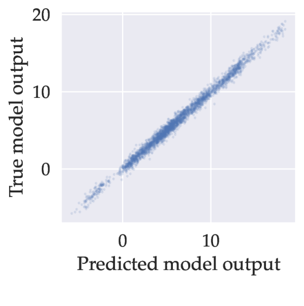
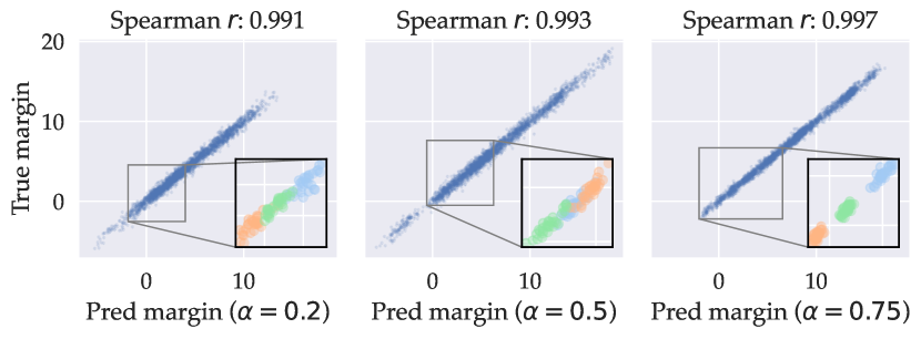
Figure 1: Datamodels predict (, x-axis) the outcome of training models on subsets of the training set sampled from and evaluating on (, y-axis) 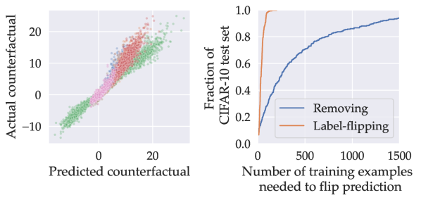
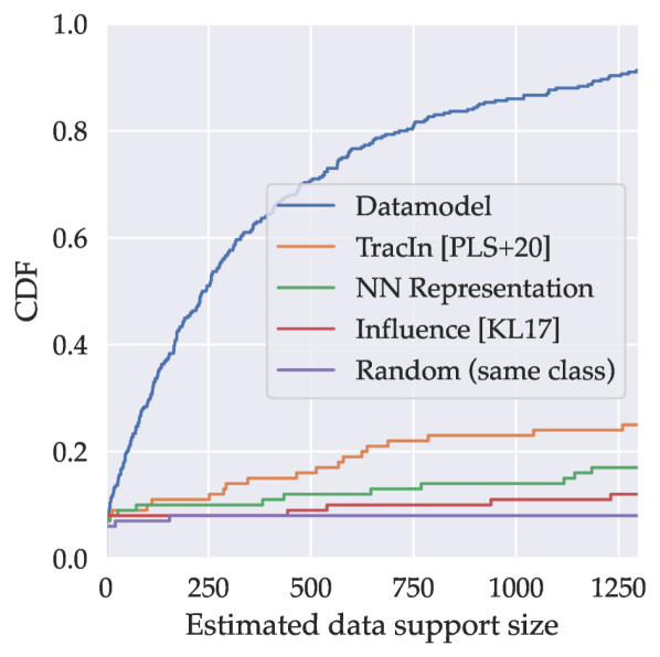
Figure 2: Datamodels predict out-of-distribution dataset counterfactuals (left) and identify brittle predictions (right). As seen on the right, approximately 50% of predictions on the CIFAR-10 test set can be flipped by removing less than (target-specific) training images. If we flip the labels of chosen training images instead of removing them, just 35 images suffices. -
•
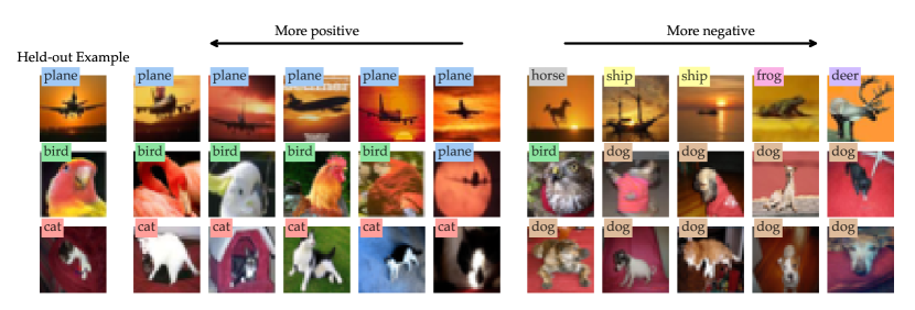
Datamodel weights encode similarity (§ 4.2, Figure 3): the most positive (resp., negative) datamodel weights tend to correspond to similar training images from the same (resp., different) class as the target example . We use this property to identify significant train-test leakage across both datasets we study (CIFAR-10 and Functional Map of the World [KSM+20a, CFW+18a]).

Figure 3: High-magnitude datamodel weights identify semantically similar training examples (top), which we can use to find train-test leakage in benchmark computer vision datasets (bottom). -
•
Datamodels yield a well-behaved embedding (§ 4.3, Figure 4): viewing datamodel weights as a feature embedding of each image into (where is the training set size), we discover a well-behaved representation space. In particular, we find that so-called datamodel embeddings:
-
(a)
enable (qualitatively) high-quality clustering;
-
(b)
allow us to identify model-relevant subpopulations that we can causally verify in a natural sense;
-
(c)
have a number of advantages over representations derived from, e.g., the penultimate layer of a fixed pre-trained network, such as higher effective dimensionality and (a priori) human-meaningful coordinates.
Figure 4: Datamodels yield a well-behaved (left), relatively dense (right) embedding of any given input into , where is the training set size. Applying natural manipulations to these embeddings enables a variety of applications which we discuss more thoroughly in § 4.3. -
(a)
More broadly, datamodels turn out to be a versatile tool for understanding how learning algorithms leverage their training data. In Section 6, we contextualize datamodeling with respect to several ongoing lines of work in machine learning and statistics. We conclude, in Section 7, by outlining a variety of directions for future work on both improving and applying datamodels.
2 Constructing (linear) datamodels
As described in Section 1, building datamodels comprises the following steps:
-
(a)
pick a parameterized class of functions ;
-
(b)
sample a collection of subsets from a fixed training set according to a distribution ;
-
(c)
for each subset , train a model using algorithm , evaluate the model on target input using the relevant metric (e.g., loss); collect the resulting pair ;
-
(d)
split the collected dataset of subset-output pairs into a datamodel training set of size , a datamodel validation set of size , and a datamodel test set of size ;
-
(e)
estimate parameters by fitting on subset-output pairs, i.e., by minimizing
over the collected datamodel training set, and use the validation set to perform model selection.
We now explicitly instantiate this framework, with the goal of understanding the predictions of (deep) classification models. To this end, we revisit steps (a)-(e) above, and consider each relevant aspect—the sampling distribution , the output function , the parameterized family , and the loss function —separately:
(a) What surrogate function should we use?
The first design choice to make is which family of parameterized surrogate functions to optimize over. At first, one might be inclined to use a complex family of functions in the hope of reducing potential misspecification error. After all, is meant to be a surrogate for the end-to-end training of a deep classifier. In this work, however, we will instantiate datamodeling by taking to be a simple linear mapping
| (5) |
where we recall that is the size- characteristic vector of within (cf. (3)).
Remark 1.
While we will allow to fit a bias term as above, for notational convenience we omit throughout this work and will simply write to represent a datamodel prediction for the set .
(b) What distribution over training subsets do we use?
In step (a) of the estimation process above, we collect a “datamodel training set” by sampling subsets from a distribution . A simple first choice for —and indeed, the one we consider for the remainder of this work—is the distribution of random -fraction subsets of the training set. Formally, we set
| (6) |
This design choice reduces the choice of to a choice of subsampling fraction , a decision whose impact we explore in Section 5. In practice, we estimate datamodels for several choices of , as it turns out that the value of corresponding to the most useful datamodels can vary by setting.
(c) What outputs should we track?
Recall that for any subset of the training set , is intended to be a specific (potentially stochastic) function representing the output of a model trained on and evaluated on a target example . There are, however, several candidates for based on which model output we opt to track.
In the context of understanding classifiers, perhaps the simplest such candidate is the correctness function (i.e., a stochastic function that is if the model trained on is correct on , and otherwise). However, while the correctness function may be a natural choice for , it turns out to be suboptimal in two ways. First, fitting to the correctness function ignores potentially valuable information about the model’s confidence in a given decision. Second, recall that our procedure fits model outputs using a least-squares linear model, which is not designed to properly handle discrete (binary) dependent variables.
A natural way to improve over our initial candidate would thus be to use continuous output function, such as cross-entropy loss or correct-label confidence. But which exact function should we choose? In Appendix C, we describe a heuristic that we use to guide our choice of the correct-class margin:
| (7) |
(e) What loss function should we minimize?
In step (d) above, we are free to pick any estimation algorithm for . This freedom of choice allows us to incorporate priors into the datamodeling process. In particular, one might expect that predictions on a given target example will not depend on every training example. We can incorporate a corresponding sparsity prior by adding regularization, i.e., setting
| (8) |
where we recall that is the size of the original training set . We can use cross-validation to select the regularization parameter for each specific target example .
3 Accurately predicting outputs with datamodels
We now demonstrate how datamodels can be applied in the context of deep neural networks—specifically, we consider deep image classifiers trained on two standard datasets: CIFAR-10 [Kri09a] and Functional Map of the World (FMoW) [KSM+20a] (see Appendix D.1 for more information on each dataset).
Goal.
As discussed in Section 1, our goal is to construct a collection of datamodels for each dataset, with each datamodel predicting the model-training outcomes for a specific target example. Thus, for both CIFAR and FMoW, we fix a deep learning algorithm (architecture, random initialization, optimizer, etc.), and aim to estimate a datamodel for each test set example and training set example. As a result, we will obtain “test set datamodels” and “training set datamodels” for CIFAR (each being a linear model parameterized by a vector , for ); as well as test set datamodels and training set datamodels for FMoW (again, parameterized by where ).
3.1 Implementation details
Before applying datamodels to our two tasks of interest, we address a few remaining technical aspects of datamodel estimation:
Simultaneously estimating datamodels for a collection of target examples.
Rather than repeat the entire datamodel estimation process for each target example of interest separately, we can estimate datamodels for an entire set of target examples simultaneously through model reuse. Specifically, we train a large pool of models on subsets sampled from the distribution , and use the same models to compute outputs for each target example .
Collecting a (sufficiently large) datamodel training set.
The cost of obtaining a single subset-output pair can be non-trivial—in our case, it involves training a ResNet from scratch on CIFAR-10. It turns out, however, that recent advances in fast neural network training [Pag18a, LIE+22a] allow us to train a wealth of models on different -subsets of each dataset very efficiently. (For example, for we can use [LIE+22a] to train 40,000 models/day on an GPU machine; see Appendix D.2 for details.) We train CIFAR models and FMoW models on subsets of each dataset. We also train models for each subsampling fraction , using to scale . See Table 1 for a summary of the models trained.
| Models trained | ||
| Subset size () | CIFAR-10 | FMoW |
| 0.1 | 1,500,000 | – |
| 0.2 | 750,000 | 375,000 |
| 0.5 | 300,000 | 150,000 |
| 0.75 | 600,000 | 300,000 |
Computing datamodels when the target example is a training input.
Recall that the target example for which we estimate a datamodel can be arbitrary. In particular, could itself be a training example—indeed, as we mention above, our goal is to estimate a datamodel for every image in the FMoW and CIFAR-10 test and training sets. When is in the training set, however, we slightly alter the datamodel estimation objective (8) to exclude training sets containing the target example:
| (9) |
Running LASSO regression at scale.
After training the models, we record the correct-class margin for all the (train and test) images as well as the training subsets. Our task now is to estimate, for each example in the train and test set, a datamodel mapping subsets to observed margins. Recall that we compute datamodels via -regularized least-squares regression (cf. (8)), where we set the regularization parameter for each test image independently via a fixed validation set of trained models.
However, most readily available LASSO solvers require too much memory or are prohibitively slow for our values of (the number of datamodels to estimate), (the number of models trained and thus the size of the datamodel training set of subset-output pairs), and (the size of the original tasks training set and thus the input dimensionality of the regression problem in (8)). We therefore built a custom solver leveraging the works of [WSM21a] and [LIE+22a]—details of our implementation are in Appendix E.1.
3.2 Results: linear datamodels can predict deep network training
For both datasets considered (CIFAR-10 and FMoW), we minimize objectives (8) (respectively, (9)) yielding a datamodel for each example in the test set (respectively, training set). We now assess the quality of these datamodels in terms of how well they predict model outputs on unseen subsets (i.e., fresh samples from ). We refer to this process as on-distribution evaluation because we are interested in subsets , sampled from the same distribution as the datamodel training set, but not the exact ones used for estimation. (In fact, recall that we explicitly held out subset-output pairs for evaluation in Section 2.)
We focus here on the collection of datamodels corresponding to the CIFAR-10 test set, i.e., a set of linear datamodel parameters corresponding to examples for (analogous results for FMoW are in Section E.2). In Figure 6, aggregating over both datamodels and heldout subsets , we compare datamodel predictions to expected true model outputs (which we estimate by training 100 models on the same subset and averaging their output on ). The results show a near-perfect correspondence between datamodel predictions and ground truth. Thus, for a given target example , we can accurately predict the outcome of “training a neural network on a random (-)training subset and computing correct-class margin on ” (a process that involves hundreds of SGD steps on a non-convex objective) as a simple linear function of the characteristic vector of the subset.
Sample complexity.
We next study the dependence of datamodel estimation on the size of the datamodel training set . Specifically, we can measure the on-distribution average mean-squared error (MSE) as
| (10) |
To evaluate (10), we replace the inner expectation with an empirical average, again using a heldout set of samples that was not used for estimation.
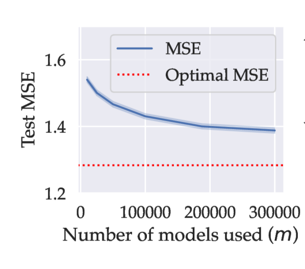
In Figure 6, we plot average MSE as a function of the number of trained models . To put the results into context, we introduce the optimal mean-squared error loss (OPT), which is the MSE (10) with datamodel predictors replaced by the optimal deterministic predictors :
| (11) |
Note that OPT is independent of the estimator and measures only the inherent variance in the prediction problem, i.e., loss that will necessarily be incurred due only to inherent noise in deep network training.
The role of regularization.
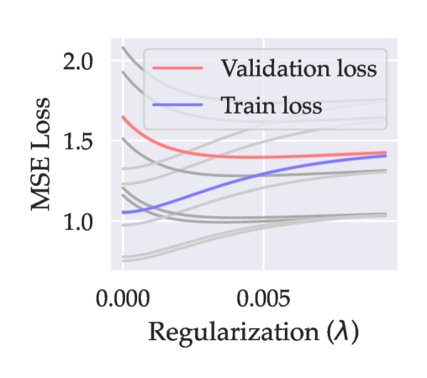
Finally, in Appendix E.2, we study the effect of the regularization parameter (cf. (8) and (9)) on datamodel performance. In particular, in Figure 19 we plot the variation in average MSE, on both on-distribution subsets (i.e., the exact subsets that we used to optimize (8)) and unseen subsets, as we vary the regularization parameter in (8). We find that—as predicted by classical learning theory—setting leads to overfit datamodels, i.e., estimators that perform well on the exact subsets that were used to estimate them, but are poor output predictors on new subsets sampled from . (In fact, using trained models with results in higher MSE than using only with optimal , i.e., the left-most datapoint in Figure 1).
4 Leveraging datamodels
Now that we have introduced (Section 1), instantiated (Section 2), and implemented (Section 3) the datamodeling framework, we turn to some of its applications. Specifically, we will now show how to apply datamodels within three different contexts:
Counterfactual prediction.
We originally constructed datamodels to predict the outcome of training a model on random (-)subsets of the training set. However, it turns out that we can also use datamodels to predict model outputs on arbitrary subsets (i.e., subsets that are “off-distribution” from the perspective of the datamodel prediction task). To illustrate the utility of this capability, we will use datamodels to (a) identify predictions that are brittle to removal of relatively few training points, and (b) estimate data counterfactuals, i.e., the causal effects of removing groups of training examples.
Train-test similarity.
We demonstrate that datamodels can identify, for any given target example , a set of visually similar examples in the training data. Leveraging this ability, we will identify instances of train-test leakage, i.e., when test examples are duplicated (or nearly duplicated) within the training set.
Data embeddings.
We show that for a given target example with corresponding datamodel , we can use the parameters of the datamodel as an embedding of the target example into (where is the training set size). By applying two standard data exploration techniques to such embeddings, we demonstrate that they capture latent structure within the data, and enable us to find model-relevant data subpopulations.
4.1 Counterfactual prediction
So far, we have computed and evaluated datamodels entirely within a supervised learning framework. In particular, we constructed datamodels with the goal of predicting the outcome of training on random subsets of the training set (sampled from a distribution (6)) and evaluating on a fixed target example . Accordingly, for each target example , we evaluated its datamodel by (a) sampling new random subsets (from the same distribution); (b) training (a neural network) on each one of these subsets; (c) measuring correct-class margin on the target example ; and (d) comparing the results to the datamodel’s predictions (namely, ) in terms of expected mean-squared error (see (10)) over the distribution of subsets.
We will now go beyond this framework, and use datamodels to predict the outcome of training on arbitrary subsets of the training set. In particular, consider a fixed target example with corresponding datamodel . For any subset of the training set , we will use the datamodel-predicted outcome of training on and evaluating on , i.e., in place of the ground-truth outcome Since is an arbitrary subset of the training set, it is “out-of-distribution” with respect to the distribution of fixed-size subsets that we designed the datamodel to operate on. As such, using datamodel predictions in place of end-to-end-model training in this manner is not a priori guaranteed to work. Nevertheless, we will demonstrate through two applications that datamodels can in fact be effective proxies for end-to-end model training, even for such out-of-distribution subsets.
[Proxy for end-to-end training] We can use datamodel predictions as an efficient, closed-form proxy for end-to-end model training. That is, for a test example with datamodel , and an arbitrary subset of the training set , we can leverage the approximation
4.1.1 Measuring brittleness of individual predictions to training data removal
We first illustrate the utility of datamodels as a proxy for model training by using them to answer the question: how brittle are model predictions to removing training data? While all useful learning algorithms are data-dependent, cases where model behavior is sensitive to just a few data points are often of particular interest or concern [BGM21a, DKM+06a]. To quantify such sensitivity, we define the data support of a target example as
| (12) |
Intuitively, examples with a small data support are the examples for which removing a small subset of the training data significantly changes model behavior, i.e., they are “brittle” examples by our criterion of interest. By computing for every image in the test set, we can thus get an idea of how brittle model predictions are to removing training data.
Computing data support.
One way to compute for a given target example would be to train several models on every possible subset of the training set , then report the largest subset for which the example was misclassified on average—the complement of this set would be exactly . However, exhaustively computing data support in this manner is simply intractable.
Using datamodels as a proxy for end-to-end model training provides an (efficient) alternative approach. Specifically, rather than training models on every possible subset of the training set, we can use datamodel-predicted outputs to perform a guided search, and only train on subsets for which predicted margin on the target example is small. This strategy (described in detail in Algorithm 1 and in Appendix F.3) allows us to compute estimates of the data support while training only a handful of models per target example.
Results.
We apply our algorithm to estimate for 300 random target examples in the CIFAR-10 test set. For over 90% of these 300 examples, we are able to certify that our estimated data support is strictly larger than the true data support (i.e., that we are not over-estimating brittleness) by training several models after excluding the estimated data support and checking that the target example is indeed misclassified on average.
We plot the distribution of estimated data support sizes in Figure 7. Around half of the CIFAR-10 test images have a datamodel-estimated data support comprising 250 images or less, meaning that removing a specific 0.4% of the CIFAR-10 training set induces misclassification. Similarly, 20% of the images had an estimated data support of less than 40 training images (which corresponds to 0.08% of the training set).
Baselines.
To contextualize these findings, we compare our estimates of data support to a few natural baselines. We provide the exact comparison setup in Appendix F.3.1: in summary, each baseline technique can be cast as a swap-in alternative to datamodels for guiding the data support search described above.
It turns out that every baseline we tested provides much looser estimates of data support (Figure 7). For example, even the best-performing baseline predicts that one would need to remove over 600 training images per test image to force misclassification on 20% of the test set444Moreover, the data support estimates derived from the baselines are only “certifiable” in the above-described sense (see the beginning of the “Results” paragraph) for 60% of the 300 test examples we study (as opposed to 90% for datamodel-derived estimates).. In contrast, our datamodel-guided estimates indicate that removing 40 train examples is sufficient for misclassifying 20% of test examples.
Removing versus mislabeling.
Note that the brittleness we consider in this section (i.e., brittleness to removing training examples) is substantively different than brittleness to mislabeling examples (as in label-flipping attacks [KL17a, XXE12a, RWR+20a]). In particular, brittleness to removal indicates that there exists a small set of training images whose presence is necessary for correct classification of the target example (thus motivating the term “data support”). Meanwhile, label-flipping attacks can succeed even when the target example has a large data support, as (consistently) mislabeling a set of training examples provide a much stronger signal than simply removing them. Nevertheless, we can easily adapt the above experiment to test brittleness to mislabeling—we do so in Appendix F.4. As one might expect, test predictions are even more brittle to data mislabeling than removal—for 50% of the CIFAR-10 test set, mislabeling 35 target-specific training examples suffices to flip the corresponding prediction (see Figure 24 for a CDF).
4.1.2 Predicting data counterfactuals
As we have already seen, a simple application of datamodels as a proxy for model training (on arbitrary subsets of the training set) enabled us to identify brittle predictions. We now demonstrate another, more intricate application of datamodels as a proxy for end-to-end training: predicting data counterfactuals.
For a fixed target example , and a specific subset of the training set , a data counterfactual is the causal effect of removing the set of examples on model outputs for . In terms of our notation, this effect is precisely
Such data counterfactuals can be helpful tools for finding brittle predictions (as in the previous subsection), estimating group influence (as done by [KAT+19a] for linear models), and more broadly for understanding how training examples combine (through the lens of the model class) to produce test-time predictions.
Estimating data counterfactuals.
Just as in the last section, we again use datamodels beyond the supervised learning regime in which they were developed. In particular, we predict the outcome of a data counterfactual as
where again is the datamodel for a given target example of interest. Since is a linear function in our case, the above predicted data counterfactual actually simplifies to
Our goal now is to demonstrate that datamodels are useful predictors of data counterfactuals across a variety of removed sets . To accomplish this, we use a large set of target examples. Specifically, for each such target example, we consider different subset sizes ; for each such , we use a variety of heuristics to select a set comprising “examples of interest.” These heuristics are:
- (a)
-
(b)
setting to be the maximizer of the datamodel-predicted counterfactual, i.e.,
(Note that since our datamodels are linear, this simplifies to excluding the training examples corresponding to the top coordinates of the datamodel parameter .)
-
(c)
setting to be the training images corresponding to the bottom (i.e., most negative) coordinates of the datamodel weight .
We consider six values of (the size of the removed subset) ranging from to examples (i.e., of the training set). Thus, the outcome of our procedure is, for each target example, both true and datamodel-predicted data counterfactuals for 30 different training subsets (six values of and five different heuristics).
Results.
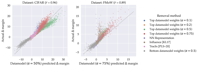
In Figure 8, we plot datamodel-predicted data counterfactuals against true data counterfactuals, aggregating across all target examples , values of , and selection heuristics for . We find a strong correlation between these two quantities. In particular, across all factors of variation, predicted and true data counterfactuals have Spearman correlation and for CIFAR-10 and FMoW respectively. In fact, the two quantities are correlated roughly linearly: we obtain (Pearson) correlations of (CIFAR-10) and (FMoW) between counterfactuals and their estimates on aggregate. Correlations are even more pronounced when restricting to any single class of removed sets (i.e., any single hue in Figure 8).
Limits of datamodel predictions.
We have seen that datamodels accurately predict the outcome of many natural data counterfactuals, despite only being constructed to predict outcomes for random subsets of a fixed size ( for and the training set size). Of course, due to both estimation error (i.e., we might not have trained enough models to identify optimal linear datamodels) and misspecification error (i.e., the optimal datamodel might not be linear), we don’t expect a perfect correspondence between datamodel-predicted outputs and true outputs for all possible subsets of the training set. Indeed, this is part of the reason why we estimated datamodels for several values of , only one of which is shown in Figure 8. As shown in Appendix F.9, datamodels estimated for other values of still display strong correlation between true and predicted model outputs, but behave qualitatively differently than the ones shown above (i.e., each value of is better or worse at predicting the outcomes of certain types of counterfactuals).
4.2 Using datamodels to find similar training examples
We now turn to another application of datamodels: identifying training examples that are similar to a given test example. One can use this primitive to identify issues in datasets such as duplicated training examples [LIN+21a] or train-test leakage [BD20a] (test examples that have near-duplicates in the training set).
Recall that in our instantiation of the framework, datamodels predict model output (for a fixed target example) as a linear function of the presence of each training example in the training set. That is, we predict the output of training on a subset of the training set as
A benefit of parameterizing datamodels as simple linear functions is that we can use the magnitude of the coordinates of to ascertain feature importance [GE03a]. In particular, since in our case each feature coordinate (i.e., each coordinate of ) actually represents the presence of a particular training example, we can interpret the highest-magnitude coordinates of as the indices of the training examples whose presence (or absence) is most predictive of model behavior (again, on the fixed target example in context).
We now show that these high-magnitude training examples (a) they visually resemble the target image, yielding a method for finding similar training examples to a given target; and (b) as a result, datamodels can automatically detect train-test leakage. {appmode}[Train-test similarity] For a test example with a linear datamodel , we can interpret the training examples corresponding to the highest-magnitude coordinates of as the “nearest neighbors” of .
4.2.1 Finding similar training examples
Motivated by the feature importance perspective described above, we visualize (in Figures 9 and 33) a random set of target examples from the CIFAR-10 test set together with the CIFAR-10 training images that correspond to the highest-magnitude datamodel coordinates for each test image.
Results.
We find that for a given target example, the highest-magnitude datamodel coordinates—both positive and negative—consistently correspond to visually similar training examples.
Furthermore, the exact training images that are surfaced by looking at high-magnitude weights differ depending on the subsampling parameter that we use while constructing the datamodels. (Recall from Section 2 that controls the size of the random subsets used to collect the datamodel training set—a datamodel estimated with parameter is constructed to predict outcomes of training on random training subsets of size , where is the training set size.) In Figure 10 (and 34), we consider a pair of target examples from the CIFAR-10 test set, and, for each target example, compare the top training images from two different datamodels: one estimated using , and the other using . We find that in some cases (e.g., Figure 10 left), the datamodel identifies training images that are highly similar to the target example but do not correspond to the highest-magnitude coordinates for the datamodel (in other cases, the reverse is true). Our hypothesis here—which we expand upon in Section 5—is that datamodels estimated with lower (i.e., based on smaller random training subsets) find train-test relationships driven by larger groups of examples (and vice-versa).

Influence functions.
Another method for finding similar training images is influence functions, which aim to estimate the effect of removing a single training image on the loss (or correctness) for a given test image. A standard technique from robust statistics [HRR+11a] (applied to deep networks by [KL17a]) uses first-order approximation to estimate influence of each training example. We find (cf. Appendix Figure 35), that the high-influence and low-influence examples yielded by this approximation (and similar methods) often fail to find similar training examples for a given test example (also see [BPF21a, HYH+21a]).
4.2.2 Identifying train-test leakage
We now leverage datamodels’ ability to surface training examples similar to a given target in order to identify same-scene train-test leakage: cases where test examples are near-duplicates of, or clearly come from the same scene as, training examples. Below, we use datamodels to uncover evidence of train-test leakage on both CIFAR and FMoW, and show that datamodels outperform a natural baseline for this task.
Train-test leakage in CIFAR.
To find train-test leakage in CIFAR-10, we collect ten candidate training examples for each image in the CIFAR-10 test set—the ones corresponding to the ten largest coordinates of the test example’s datamodel parameter. We then show crowd annotators (using Amazon Mechanical Turk) tasks that consist of a random CIFAR-10 test example accompanied by its candidate training examples. We ask the annotators to label any of the candidate training images that constitute instances of same-scene leakage (as defined above). We show each task (i.e., each test example) to multiple annotators, and compute the “annotation score” for each of the test example’s candidate training examples as the fraction of annotators who marked it as an instance of leakage. Finally, we compute the “leakage score” for each test example as the highest annotation score (over all of its candidate train images). We use the leakage score as a proxy for whether or not the given image constitutes train-test leakage.
In Figure 11, we plot the distribution of leakage scores over the CIFAR-10 test set, along with random train-test pairs stratified by their annotation score. As the annotation score increases, pairs (qualitatively) appear more likely to correspond to leakage (see Appendix H for more pairs). Furthermore, roughly 10% of test set images were labeled as train-test leakage by over half of the annotators that reviewed them.

Train-test leakage in FMoW.
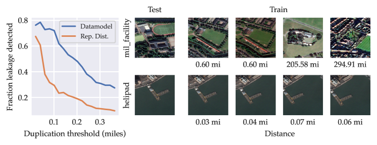
To identify train-test leakage on FMoW, we begin with the same candidate-finding process that we used for CIFAR-10. However, FMoW differs from CIFAR in that the examples (satellite images labeled by category, e.g., “port” or “arena”) are annotated with geographic coordinates. These coordinates allow us to avoid crowdsourcing—instead, we compute the geodesic distance between the test image and each of the candidates, and use a simple threshold (in miles) to decide whether a given test example constitutes train-test leakage.
Furthermore, we can calculate a “ground-truth” number of train-test leakage instances by counting the test examples whose geodesic nearest-neighbor in the training set is within the specified threshold .666 It turns out that despite having already been de-duplicated, about 20% and 80% of FMoW test images are within 0.25 and 2.6 miles of a training image, respectively—see Appendix Figure 40. Comparing this ground truth to the number of instances of leakage found within the candidate examples yields a qualitative measure of the efficacy of our method (i.e., the quality of candidates we generate).
In Figure 12, we plot this measure of efficacy (# instances found / # ground truth) as a function of the threshold , and also visualize examples images from the FMoW test set together with their corresponding datamodel-identified training set candidates. To put our quantitative results into context, we compare the efficacy of candidates derived from top datamodel coordinates (i.e., the ones we use here and for CIFAR-10) to that of candidates derived from nearest neighbors in the representation space of a pretrained neural network [BCV13a, ZIE+18a] (examining such nearest neighbors is a standard way of finding train-test leakage, e.g., used by [BD20a] to study CIFAR-10 and CIFAR-100). Datamodels consistently outperform this baseline.
4.3 Using datamodels as a feature embedding
Sections 4.1 and 4.2 illustrate the utility of datamodels on a per-example level, i.e., for predicting the outcome of training on arbitrary training subsets and evaluating on a specific target example, or for finding similar training images (again, to a specific target). We’ll conclude this section by demonstrating that datamodels can also help uncover global structure in datasets of interest.
Key to this capability is the following shift in perspective. Consider a target example with corresponding linear datamodel , and recall that the datamodel is parameterized by a vector , where is the training set size. We optimized to minimize the squared-error of (8) when predicting the outcome of training on random training subsets and evaluating on the target . Now, however, instead of viewing the vector as just a parameter of the predictor , we cast it as a feature representation for the target example itself, i.e., a datamodel embedding of into . Since the datamodel is a linear function of the presence of each point in the training set, each coordinate of this “datamodel embedding” corresponds to a weight for a specific training example. One can thus think of a datamodel embedding as a feature vector that represents a target example in terms of how predictive each training example is of model behavior on .
Critically, the coordinates of a datamodel embedding have a consistent interpretation across datamodel embeddings, even for different target examples. That is, we expect similar target examples to be acted upon similarly by the training set, and thus have similar datamodel embeddings. In the same way, if model performance on two unrelated target examples is driven by two disjoint sets of training examples, their datamodel embeddings will be orthogonal. This intuition suggests that by embedding an entire dataset of examples as a set of feature vectors , we may be able to uncover structure in the set of examples by looking for structure in their datamodel embeddings, i.e., in the (Euclidean) space .
In this section we demonstrate, through two applications, the potential for such datamodel embeddings to discover dataset structure in this way. In Section 4.3.2, we use datamodel embeddings to partition datasets into disjoint clusters, and in Section 4.3.1 we use principal component analysis to get more fine-grained insights into dataset structure. To emphasize our shift in perspective (i.e., from being just a parameter of a datamodel , to being an embedding for the target example ), we introduce an embedding function which maps a particular target example to the weights of its corresponding datamodel.
[Datamodel embeddings] We can use datamodels as a way to embed any given target example into the same (Euclidean) space , where is the training set size. Specifically, we can define the datamodel embedding for a target example as the weight vector of the datamodel corresponding to .
4.3.1 Spectral clustering with datamodel embeddings
We begin with a simple application of datamodel embeddings, and show that they enable high-quality clustering. Specifically, given two examples and , datamodel embeddings induce a natural similarity measure between them:
| (13) |
where we recall that is the datamodel embedding function mapping target examples to the weights of their corresponding datamodels, and is any kernel function (below, we use the RBF kernel)777A kernel function is a similarity measure that computes the inner product between its two arguments in a transformed inner product space (see [SC04a] for an introduction). The RBF kernel is . Taking this even further, for a set of target examples , we can compute a full similarity matrix , whose entries are
| (14) |
Finally, we can view this similarity matrix as an adjacency matrix for a (dense) graph connecting all the examples : the edge between two examples will be , which is in turn the kernelized inner product between their two datamodel weights. We expect similar examples to have high-weight edges between them, and unrelated examples to have (nearly) zero-weight edges between them.
Such a graph unlocks a myriad of graph-theoretic tools for exploring datasets through the lens of datamodels (e.g., cliques in this graph should be examples for which model behavior is driven by the same subset of training examples). However, a complete exploration of these tools is beyond the scope of our work: instead, we focus on just one such tool: spectral clustering.
At a high level, spectral clustering is an algorithm that takes as input any similarity graph as well as the number of clusters , and outputs a partitioning of the vertices of into disjoint subsets, in a way that (roughly) minimizes the total weight of inter-cluster edges. We run an off-the-shelf spectral clustering algorithm on the graph induced by the similarity matrix above for the images in the CIFAR-10 test set. The result (Figure 13 and Appendix I) demonstrates a simple unsupervised method for uncovering subpopulations in datasets.

4.3.2 Analyzing datamodel embeddings with PCA
We observed above that datamodel embeddings encode enough information about their corresponding examples to cluster them into (at least qualitatively) coherent groups. We now attempt to gain even further insight into the structure of these datamodel embeddings, in the hopes of shedding light on the structure of the underlying dataset itself.
Datamodel embeddings are both high-dimensional and sparse, making analyzing them directly (e.g., by looking at the variation of each coordinate) a daunting task. Instead, we leverage a canonical tool for finding structure in high-dimensional data: principal component analysis (PCA).
PCA is a dimensionality reduction technique which—given a set of embeddings and any —returns a transformation function that maps any embedding to a new embedding , such that:
-
(a)
each of the coordinates of the transformed embeddings is a (fixed) linear combination of the coordinates of the initial datamodel embeddings, i.e., for a fixed matrix ;
-
(b)
transformed embeddings preserve as much information as possible about the original ones. More formally, we find the matrix that allows us to reconstruct the given set of embeddings from their transformed counterparts with minimal error.
Note that in (a), the -th coordinate of a transformed embedding is always the same linear combination of the corresponding original embedding (and thus, each coordinate of the transformed embedding has a concrete interpretation as a weighted combination of datamodel coefficients). The exact coefficients of this combination (i.e., the rows of the matrix above) are called the first principal components of the dataset.
We apply PCA to the collection of datamodel embeddings for the CIFAR-10 training set, and use the result to to compute new -dimensional embeddings for each target example in both the training set and the test set (i.e., by computing each target example’s datamodel embedding then transforming it to an embedding in ). We can then look at each coordinate in the new, much more manageable (-dimensional) embeddings.888We first normalize each datamodel embedding before transforming them (i.e., we transform ).
Coordinates identify subpopulations.
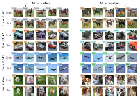
Our point of start in analyzing these transformed embeddings is to examine each transformed coordinate separately. In particular, in Figure 14 we visualize, for a few sample coordinate indices , the target examples whose transformed embeddings have particularly high or low values of the given coordinate (equivalently, these are the target examples whose datamodel embeddings have the highest or lowest projections onto the -th principal component). We find that:
-
(a)
the examples whose transformed embeddings have a large -th coordinate all (visually) share a common feature: e.g., the first-row images in Figure 14 share similar pose and color composition;
-
(b)
this (visual) feature is consistent across both train and test set examples999Recall that we computed the PCA transformation to preserve the information in only the training set datamodel embeddings. Thus, this result suggests that the transformed embeddings computed by PCA are not “overfit” to the specific examples that we used to compute it.; and
-
(c)
for a given coordinate, the most positive images and most negative images (i.e., the left and right side of each row of Figure 14, respectively) either (a) have a differing label but share the same common feature or (b) have the same label but differ along the relevant feature.
Principal components are model-faithful.
In Appendix J, we verify that not only are the groups of images found by PCA visually coherent, they are in fact rooted in how the model class makes predictions. In particular, we show that one can find, for any coordinate of the transformed embedding, the training examples that are most important to that coordinate. Furthermore, retraining without these examples significantly decreases (increases) accuracy on the target examples with the most positive (negative) coordinate , suggesting that the identified principal components actually reflect model class behavior.
4.3.3 Advantages over penultimate-layer embeddings
In the context of deep neural networks, the word “embedding” typically refers to features extracted from the penultimate layer of a fixed pre-trained model (see [BCV13a] for an overview). These “deep representations” can serve as an effective proxy for visual similarity [BD20a, ZIE+18a], and also enable a suite of applications such as clustering [GGT+17a] and feature visualization [OMS17a, EIS+19a, ARS+15a, BBC+07a].
Here, we briefly discuss a few advantages of datamodel-based embeddings over their standard penultimate layer-based counterparts.
-
•
Axis-alignment: datamodel embeddings are axis-aligned—each embedding component directly corresponds to index into the training set, as opposed to a more abstract or qualitative concept. As a corollary, aggregating or comparing different datamodel embeddings for a given dataset is straightforward, and does not require any alignment tools or additional heuristics. This is not the case for network-based representations, for which the right way to combine representations—even for two models of the same architecture—is still disagreed upon [KNL+19a, BNB21a]. In particular, we can straightforwardly compare datamodel embeddings across different target examples, model architectures, training paradigms, or even datamodel estimation techniques—as long as the set of training examples being stays the same, any resulting datamodel has a uniform interpretation.
-
•
Richer representation: the space of datamodel embeddings seems significantly richer than that of standard representation space. In particular, Appendix Figure 43 shows that for standard representation space, ten linear directions suffice to capture 90% of the variation in training set representations. The “effective dimension” of datamodel representations is much higher, with the top 500 principal components explaining only 50% of the variation in training set datamodel embeddings. This difference manifests qualitatively when we redo our PCA study on standard representations (Appendix Figure 46): principal components beyond the 10th lack both the perceptual quality and train-test consistency exhibited by those of datamodel embeddings (e.g., for datamodels even the 76th principal component, shown in Figure 14, exhibits these qualities).
-
•
Ingrained causality: datamodel embeddings inherently encode information about how the model class generalizes. Indeed, in Section 4.3.2 we verified via counterfactuals that insights extracted from the principal components of actually reflect underlying model class behavior.
5 Discussion: The role of the subsampling fraction

We have used datamodels estimated using several choices of the subsampling fraction , and saw that the value of corresponding to the most useful datamodels can vary by setting. In particular, the visualizations in Figure 10 suggest that datamodels estimated with lower (i.e., based on smaller random training subsets) find train-test relationships driven by larger groups of examples (and vice-versa). Here, we explore this intuition further using thought experiment, toy example, and numerical simulation. Our goal is to intuit how different choices of can lead to substantively different datamodels.
First, consider the task of estimating a datamodel for a prototypical image —for example, a plane on a blue sky background. As , the sets sampled from are relatively large—if these sets have enough other images of planes on blue skies, we will observe little to no variation in , since any predictor trained on will perform very well on . As a result, a datamodel for estimated with may assign very little weight to any particular image, even if in reality their total effect is actually significant.
Decreasing , then, offers a solution to this problem. In particular, we allow the datamodel to observe cases where entire groups of training examples are not present, and re-distribute the corresponding effect back to the constituents of the group (i.e., assigning them all a share of the weight).
Now, consider a highly atypical yet correctly classified example, whose correctness relies on just the presence of just a few images from the training set. In this setting, datamodels estimated with a small value of may be unable to isolate these training points, since they will constantly distribute variation in among a large group of non-present images. Meanwhile, using a large value of allows the estimated datamodel to place weight on the correct training images (since will be classified correctly until some of the important training images are not present in ).
In line with this intuition, decreasing in Figure 15 (i.e., moving from right to left) leads to datamodels that assign weight to increasingly large neighborhoods of points around the target input. This example and the above reasoning lead us to hypothesize that larger (respectively, smaller) are better-suited to cases where model predictions are driven by smaller (respectively, larger) groups of training examples. In Appendix B, we perform a more quantitative analysis of the role of , this time by studying an underdetermined linear regression model on data that is organized into overlapping subpopulations. Our findings in this setting (see Figure 16) mirror our intuition thus far—in particular, smaller values of result in datamodels that were more predictive on larger subpopulations in the training set, whereas higher values of tended to work better smaller subpopulations.
6 Related work
Datamodels build on a rich and growing body of literature in machine learning, statistics, and interpretability. In this section, we illustrate some of the connections to these fields, highlight a few of the most closely related works to ours.
6.1 Connecting datamodeling to empirical influence estimation
We start by discussing the particularly important connection between datamodels and another well-studied concept that has recently been applied to the machine learning setting: influence estimators. In particular, a recent line of work aims to compute the empirical influence [HRR+11a] of training points on predictions , i.e.,
where randomness is taken over the training algorithm. Evaluating these influence functions naively requires training models where is again the size of the train set and is the number of samples necessary for an accurate empirical estimate of the probabilities above. To circumvent this prohibitive sample complexity, a recent line of work has proposed approximation schemes for . We discuss these approximations (and their connection to our work) more generally in Section 6.2, but here we focus on a specific approximation used by [FZ20a] (and in a similar form, by [GZ19a] and [JDW+19a])101010In fact, (15) is ubiquitous—e.g., in causal inference, it is called the average treatment effect of training on on the correctness of .:
| (15) |
This estimator improves sample efficiency by reusing the same set of models to compute influences between different input pairs. More precisely, [FZ20a] show that the size of the random subsets trades off sample efficiency (model reuse is maximized when the subsets are exactly half the size of the training set, since this maximizes the number of samples available to estimate each term in (15)) and accuracy with respect to the true empirical influence (which is maximized as the subsets get larger). Despite its different goal, formulation, and estimation procedure, it turns out that we can cast the difference-of-probabilities estimator (15) above as a rescaled datamodel (in the infinite-sample limit). In particular, in Appendix K.1 we show:
lemmaatelinear Fix a training set of size , and a test example . For , let be a random variable denoting a random 50%-subset of the the training set . Let be the estimated empirical influences (15) onto estimated using the sets . Let be the least-squares estimator of whether a particular model will get image correct, i.e.,
Then, as ,
We illustrate this result quantitatively in Appendix K and perform an in-depth study of influence estimators as datamodels. As one might expect given their different goal, influence estimates significantly underperform explicit datamodels in terms of predicting model outputs with respect to every metric we studied (Table 5, Figure 49). We then attempt to explain this performance gap and reconcile it with Lemma 6.1 in terms of the estimation algorithm (OLS vs. LASSO), scale (number of models trained), and output function (0/1 loss vs. margins).
In addition to forging a connection between datamodels and influence estimates, this result also provides an alternate perspective on the parameter . Specifically, in light of our discussion in Section 5, it suggests that may control the kinds of correlations that are surfaced by empirical influence estimates.
6.2 Other connections
Influence functions and instance-based explanations.
Above, we contrasted datamodels with empirical influence functions, which measure the counterfactual effect of removing individual training points on a given model output. Specifically, in that section and the corresponding Appendix K, we discussed the subsampled influence estimator of [FZ20a], who use influences to study the memorization behavior of standard vision models. We now provide a brief overview of a variety of other methods for influence estimation developed in prior works.
First-order influence functions are a canonical tool in robust statistics that allows one to approximate the impact of removing a data point on a given parameter without re-estimating the parameter itself [HRR+11a]. [KL17a] apply influence functions to both a variety of classical machine learning models and to penultimate-layer embeddings from neural network architectures, to trace model’s predictions back to individual training examples. In classical settings (namely, for a logistic regression model), [KAT+19a] find that influence functions are also useful for estimating the impact of groups of examples. On the other hand, [BPF21a] finds that approximate influence functions scale poorly to deep neural network architectures; and [FZ20a] argue that understanding the dynamics of the penultimate layer is insufficient for understanding deep models’ decision mechanisms. Other methods for influence approximation (or more generally, instance-level attribution) include gradient-based methods [PLS+20a] and metrics based on representation similarity [CGF+19a, YKY+18a]—see [HYH+21a] for a more detailed overview. Finally, another related line of work [GZ19a, JDW+19a, WZJ+21a] uses Shapley values [Sha51a] to assign a value to datapoints based on their contribution to some aggregate metric (e.g., test accuracy).
As discussed in Section 6.1, datamodels serve a different purpose to influence functions—the former constructs an explicit statistical model, whereas the latter measures the counterfactual value of each training point. Nevertheless, we find that wherever efficient influence approximations and datamodels are quantitatively comparable (e.g., see Section 4.1 or Appendix K) datamodels predict model behavior better.
Pixel-space surrogate models for interpretability.
Datamodels are essentially surrogate models for the function mapping training data to predictions. Surrogate models from pixel-space to predictions are popular tools in machine learning interpretability [RSG16a, LL17a, SHS+19a]. For example, LIME [RSG16a] constructs a local linear model mapping test images to model predictions. Such surrogate models try to understand, for a fixed model, how the features of a given test example change the prediction. In contrast, datamodels hold the test example fixed and instead study how the images present in the training set change the prediction.
In addition to the advantages of our data-based view stated in Section 1, datamodels have two further advantages over pixel-level surrogate models: (a) a clear notion of missingness (i.e., it is easy to remove a training example but usually hard to “remove” pixels [SLL20a, JSW+22a]); and (b) globality of predictions—pixel-level surrogate models are typically accurate within a small neighborhood of a given input in pixel space, whereas datamodels model entire distribution over subsets of the training set, and remain useful both on- and off-distribution.
Model understanding beyond fixed weights.
Recall (from Section 1) that datamodels are, in part, inspired by the fact that re-training deep neural networks using the same data and model class leads to models with similar accuracies but vastly different individual predictions. This phenomenon has been observed more broadly. For example, [SYW+21a] make this point explicitly in the context of BERT [DCL+19a] pre-trained language models. Similarly, [NB20a] make note of this non-determinism for networks trained on the same training distribution (but not the same data), while [JNB+21a] find that the same is true for networks trained on the same exact data. [DHM+20a] find that on out-of-distribution data even overall accuracy is highly random. More closely to the spirit to our work, [ZGK+21a] find that non-determinism of individual predictions poses a challenge for comparing different model architectures. (They also propose a set of statistical techniques for overcoming this challenge.) More traditionally, the non-determinism is leveraged by Bayesian [Nea96a] and ensemble methods [LPB17a], which use a distribution over model weights to improve aspects of inference such as calibration of uncertainty.
Learning and memorization.
Recent work (see [Fel19a, Cha18a, ZBH+16a, BN20a] and references therein) brings to light the interplay between learning and memorization, particularly in the context of deep neural networks. While memorization and generalization may seem to be at odds, the picture is more subtle. Indeed, [Cha18a] builds a network of small lookup tables on small vision datasets to show that purely memorization-based systems can still generalize-well. [Fel19a] suggests that memorization of atypical examples may be necessary to generalize well due to a long tail of subpopulations that arises in standard datasets. [FZ20a] find some empirical support for this hypothesis by identifying memorized images on CIFAR-100 and ImageNet and showing that removing them hurts overall generalization. Relatedly, [BBF+21a] proves that for certain natural distributions, memorization of a large fraction of data, even data irrelevant to the task at hand, is necessary for close to optimal generalization. For state of the art models, recent works (e.g., [CLK+19a, CTW+21a]) show that one can indeed extract sensitive training data, indicating models’ tendency to memorize.
Conversely, it has been observed that differentially private (DP) machine learning models—whose aim is precisely to avoid memorizing the training data—tend to exhibit poorer generalization than their memorizing counterparts [ACG+16a]. Moreover, the impact on generalization from DP is disparate across subgroups [BPS19a]. A similar effect has been noted in the context of neural network pruning [HCD+19a]. Datamodeling may be a useful tool for studying these phenomena and, more broadly, the mechanisms mapping data to predictions for modern learning algorithms.
Brittleness of conclusions.
A long line of work in statistics focuses on testing the robustness of statistical conclusions to the omission of datapoints. [BGM21a] study the robustness of econometric analyses to removing a (small) fraction of data. Their method uses a Taylor-approximation based metric to estimate the most influential subset of examples on some target quantity, similar in spirit to our use of datamodels to estimate data support for a target example (as in Figure 7). Datamodels may be a useful tool for extending such robustness analyses to the context of state-of-the-art machine learning models.
7 Future work
Our instantiation of the datamodeling framework yields both good predictors of model behavior and a variety of direct applications. However, this instantiation is fairly basic and thus leaves significant room for improvement along several axes. More broadly, datamodeling provides a lens under which we can study a variety of questions not addressed in this work. In this section, we identify (a subset of) these questions and provide connections to existing lines of work on them across machine learning and statistics.
7.1 Improving datamodel estimation
In Section 2, we outlined our basic procedure for fitting datamodels: we first sample subsets uniformly at random, then fit a sparse linear model from (the characteristic vectors of) training subsets to model outputs (margins) via regularization. We first discuss various ways in which this paradigm might be improved to yield even better predictions.
-
•
Correlation-aware estimation. One key feature of our estimation methodology is that the same set of models is used to estimate datamodel parameters for an entire test set of images at once. This significantly reduces the sample complexity of estimating datamodels but also introduces a correlation between the errors in the estimated parameters. This correlation is driven by the fact that model outputs are not i.i.d. across inputs—for example, if on a picture of a dog a given model has very large output (compared to the “average” model, i.e., if is large), the model is also more likely to have large output on another picture of a dog (as opposed to, e.g., a picture of a cat).
-
•
Confidence intervals for datamodels. In this work we have focused on attaining point estimates for datamodel parameters via simple linear regression. A natural extension to these results would be to obtain confidence intervals around the datamodel weights. These could, for example, (a) provide interval estimates for model outputs rather than simple point estimates; and (b) decide if a training input is indeed a “significant” predictor for a given test input.
-
•
Post-selection inference. Relatedly, the high input-dimensionality of our estimation problem and the sparse nature of the solutions suggests that a two-stage procedure might improve sample efficiency. In such procedures, one first selects (often automatically, e.g., via LASSO) a subset of the coefficients deemed to be “significant” for a given test example, then re-fits a linear model for only these coefficients. This two-stage approach is particularly attractive in settings where the number of subset-output pairs is less than the size of the training set being subsampled.
Unfortunately, using the data itself to perform model selection in this manner—a paradigm known as post-selection inference—violates the assumptions of classical statistical inference (in particular, that the model class is chosen independently of the data) and can result in significantly miscalibrated confidence intervals. Applying valid two-stage estimation to datamodeling would be an area for further improvement upon the protocol presented in our work.
-
•
Improving subset sampling. Recall (cf. Section 2) that our framework uses a distribution over subsets to generate the “datamodel training set.” In this paper, we fixed to be random -subsets of the training set, and used a nearest-neighbors example (see Figure 15) to provide intuition around the role of . While this design choice did yield useful datamodels, it is unclear whether this class of distributions is optimal. In particular, a long line of literature in causal inference focuses on intervention design [ES07a]; drawing upon this line of work may lead to a better choice of subsampling distribution. Furthermore, one might even go beyond a fixed distribution and instead choose subsets adaptively (i.e., based on the datamodels estimated with the previously sampled subsets) in order to reduce sample complexity.
-
•
Devising better priors. Finally, in this paper we employed simple least-squares regression with regularization (tuned through a held-out validation set). While the advantage of this rather simple prior—namely, that datamodels are sparse—is that the resulting estimation methodology is largely data-driven, one may consider incorporating domain-specific knowledge to design better priors. For instance, one can use structured-sparsity [HZM11a] to take advantage of any additional structure.
7.2 Studying generalization
Datamodels also present an opportunity to study generalization more broadly:
-
•
Understanding linearity. The key simplifying assumption behind our instantiation of the datamodeling framework is that we can approximate the final output of training a model on a subset of the trainset as a linear function of the presence of each training point. While this assumption certainly leads to a simple estimation procedure, we have very little justification for why such a linear model should be able to capture the complexities of end-to-end model training on data subsets. However, we find that datamodels can accurately predict ground-truth model outputs (cf. Sections 2). In fact, we find a tight linear correlation between datamodel predictions and model outputs even on out-of-distribution (i.e., not in the support of ) counterfactual datasets. Understanding why a simple linearity assumption leads to effective datamodels for deep neural networks is an interesting open question. Tackling this question may necessitate a better understanding of the training dynamics and implicit biases behind overparameterized training [BMR21a, SRK+20a].
-
•
Using sparsity to study generalization. A recent line of work in machine learning studies the interplay between learning, overparameterization, and memorization [Fel19a, Cha18a, ZBH+16a, BN20a, ZBH+20a]. Datamodeling may be a helpful tool in this pursuit, as it connects predictions of machine learning models directly to the data used to train them. For example, the data support introduced in Section 4.1.1 provides a quantitative measure of “how memorized” a given test input is.
-
•
Theoretical characterization of the role of . In line with our intuitions in Section 5, we have observed both qualitatively (e.g., Figure 10) and quantitatively (e.g., Appendix B) that estimating datamodels using different values of identifies correlations at varying granularities. However, despite empirical results around the clear role of —Appendix B even isolates its effect on datamodels for simple underdetermined linear regression—we lack a crisp theoretical understanding of how affects our estimated datamodels. A better theoretical understanding of the role of , even for simple models trained on structured distributions, can provide us with more rigorous intuition for the phenomena observed here, and can in turn guide the development of better choices of sampling distribution for datamodeling.
7.3 Applying datamodels
Finally, each of the presented perspectives in Section 4 can be taken further to enable even better data and model understanding. For example:
-
•
Interpreting predictions. For a given test example, the training images corresponding to the largest-magnitude datamodel weights both (a) share features in common with the test example; and (b) seem to be causally linked to the test example (in the sense that removing the training images flips the test prediction). This immediately suggests the potential utility of datamodels as a tool for interpreting test-time predictions in a counterfactual-centric manner. Establishing them as such requires further evaluation through, for example, human-in-the-loop studies.
-
•
Building data exploration tools. In a similar vein, another opportunity for future work is in building user-friendly data exploration tools that leverage datamodel embeddings. In this paper we present the simplest such example in the form of PCA, but leave the vast field of data bias and feature discovery methods (cf. [CAS+19a] and [LSI+21a] for a survey) unexplored.
8 Conclusion
We present datamodeling, a framework for viewing the output of model training as a simple function of the presence of each training data point. We show that a simple linear instantiation of datamodeling enables us to predict model outputs accurately, and facilitates a variety of applications.
Acknowledgements
We thank Chiyuan Zhang and Vitaly Feldman for providing a set of 5,000 models with which we began our investigation. We also thank Hadi Salman for valuable discussions.
Work supported in part by the NSF grants CCF-1553428 and CNS-1815221, and Open Philanthropy. This material is based upon work supported by the Defense Advanced Research Projects Agency (DARPA) under Contract No. HR001120C0015.
[sorting=nyt]
References
- [ACG+16] Martín Abadi, Andy Chu, Ian Goodfellow, H. McMahan, Ilya Mironov, Kunal Talwar and Li Zhang “Deep Learning with Differential Privacy” In Proceedings of the 2016 ACM SIGSAC Conference on Computer and Communications Security Vienna, Austria: ACM, 2016, pp. 308–318
- [ARS+15] Hossein Azizpour, Ali Sharif Razavian, Josephine Sullivan, Atsuto Maki and Stefan Carlsson “Factors of transferability for a generic convnet representation” In IEEE transactions on pattern analysis and machine intelligence, 2015
- [BPS19] Eugene Bagdasaryan, Omid Poursaeed and Vitaly Shmatikov “Differential privacy has disparate impact on model accuracy” In Neural Information Processing Systems (NeurIPS), 2019
- [BNB21] Yamini Bansal, Preetum Nakkiran and Boaz Barak “Revisiting Model Stitching to Compare Neural Representations” In Neural Information Processing Systems (NeurIPS), 2021
- [BMR21] Peter L Bartlett, Andrea Montanari and Alexander Rakhlin “Deep learning: a statistical viewpoint” In arXiv preprint arXiv:2103.09177, 2021
- [BD20] Björn Barz and Joachim Denzler “Do we train on test data? purging cifar of near-duplicates” In Journal of Imaging, 2020
- [BPF21] Samyadeep Basu, Phillip Pope and Soheil Feizi “Influence Functions in Deep Learning Are Fragile” In International Conference on Learning Representations (ICLR), 2021
- [BBC+07] Shai Ben-David, John Blitzer, Koby Crammer and Fernando Pereira “Analysis of representations for domain adaptation” In Neural Information Processing Systems (NeurIPS), 2007
- [BCV13] Y. Bengio, A. Courville and P. Vincent “Representation Learning: A Review and New Perspectives” In IEEE Transactions on Pattern Analysis and Machine Intelligence, 2013
- [BN20] Guy Bresler and Dheeraj Nagaraj “A corrective view of neural networks: Representation, memorization and learning” In Conference on Learning Theory (COLT), 2020
- [BGM21] Tamara Broderick, Ryan Giordano and Rachael Meager “An Automatic Finite-Sample Robustness Metric: Can Dropping a Little Data Change Conclusions?” In Arxiv preprint arXiv:2011.14999, 2021
- [BBF+21] Gavin Brown, Mark Bun, Vitaly Feldman, Adam Smith and Kunal Talwar “When is memorization of irrelevant training data necessary for high-accuracy learning?” In Proceedings of the 53rd Annual ACM SIGACT Symposium on Theory of Computing, 2021
- [CLK+19] Nicholas Carlini, Chang Liu, Jernej Kos, Úlfar Erlingsson and Dawn Song “The Secret Sharer: Measuring Unintended Neural Network Memorization & Extracting Secrets” In USENIX Security Symposium, 2019
- [CTW+21] Nicholas Carlini, Florian Tramer, Eric Wallace, Matthew Jagielski, Ariel Herbert-Voss, Katherine Lee, Adam Roberts, Tom Brown, Dawn Song and Ulfar Erlingsson “Extracting training data from large language models” In 30th USENIX Security Symposium (USENIX Security 21), 2021
- [CAS+19] Shan Carter, Zan Armstrong, Ludwig Schubert, Ian Johnson and Chris Olah “Activation atlas” In Distill, 2019
- [CGF+19] Guillaume Charpiat, Nicolas Girard, Loris Felardos and Yuliya Tarabalka “Input similarity from the neural network perspective” In Neural Information Processing Systems (NeurIPS), 2019
- [Cha18] Satrajit Chatterjee “Learning and Memorization” In Proceedings of the 35th International Conference on Machine Learning, 2018
- [CFW+18] Gordon Christie, Neil Fendley, James Wilson and Ryan Mukherjee “Functional Map of the World” In Proceedings of the IEEE Conference on Computer Vision and Pattern Recognition (CVPR), 2018
- [CYM+20] Cody Coleman, Christopher Yeh, Stephen Mussmann, Baharan Mirzasoleiman, Peter Bailis, Percy Liang, Jure Leskovec and Matei Zaharia “Selection via proxy: Efficient data selection for deep learning” In International Conference on Learning Representations (ICLR), 2020
- [DHM+20] Alexander D’Amour, Katherine A. Heller, Dan Moldovan, Ben Adlam, Babak Alipanahi, Alex Beutel, Christina Chen, Jonathan Deaton, Jacob Eisenstein, Matthew D. Hoffman, Farhad Hormozdiari, Neil Houlsby, Shaobo Hou, Ghassen Jerfel, Alan Karthikesalingam, Mario Lucic, Yi-An Ma, Cory Y. McLean, Diana Mincu, Akinori Mitani, Andrea Montanari, Zachary Nado, Vivek Natarajan, Christopher Nielson, Thomas F. Osborne, Rajiv Raman, Kim Ramasamy, Rory Sayres, Jessica Schrouff, Martin Seneviratne, Shannon Sequeira, Harini Suresh, Victor Veitch, Max Vladymyrov, Xuezhi Wang, Kellie Webster, Steve Yadlowsky, Taedong Yun, Xiaohua Zhai and D. Sculley “Underspecification Presents Challenges for Credibility in Modern Machine Learning” In Arxiv preprint arXiv:2011.03395, 2020
- [DDP19] Constantinos Daskalakis, Nishanth Dikkala and Ioannis Panageas “Regression from dependent observations” In Proceedings of the 51st Annual ACM SIGACT Symposium on Theory of Computing, 2019, pp. 881–889
- [DCL+19] Jacob Devlin, Ming-Wei Chang, Kenton Lee and Kristina Toutanova “Bert: Pre-training of deep bidirectional transformers for language understanding” In Conference of the North American Chapter of the Association for Computational Linguistics (ACL), 2019
- [DT17] Terrance DeVries and Graham W Taylor “Improved Regularization of Convolutional Neural Networks with Cutout” In arXiv preprint arXiv:1708.04552, 2017
- [DKM+06] Cynthia Dwork, Krishnaram Kenthapadi, Frank McSherry, Ilya Mironov and Moni Naor “Our data, ourselves: Privacy via distributed noise generation” In Annual International Conference on the Theory and Applications of Cryptographic Techniques, 2006
- [ES07] Frederick Eberhardt and Richard Scheines “Interventions and Causal Inference” In Philosophy of Science, 2007
- [EIS+19] Logan Engstrom, Andrew Ilyas, Shibani Santurkar, Dimitris Tsipras, Brandon Tran and Aleksander Madry “Adversarial Robustness as a Prior for Learned Representations” In ArXiv preprint arXiv:1906.00945, 2019
- [Fel19] Vitaly Feldman “Does Learning Require Memorization? A Short Tale about a Long Tail” In Symposium on Theory of Computing (STOC), 2019
- [FZ20] Vitaly Feldman and Chiyuan Zhang “What Neural Networks Memorize and Why: Discovering the Long Tail via Influence Estimation” In Advances in Neural Information Processing Systems (NeurIPS) 33, 2020, pp. 2881–2891
- [FHT10] Jerome Friedman, Trevor Hastie and Rob Tibshirani “Regularization paths for generalized linear models via coordinate descent” In Journal of statistical software, 2010
- [GGS19] Nidham Gazagnadou, Robert M Gower and Joseph Salmon “Optimal mini-batch and step sizes for SAGA” In International Conference on Machine Learning (ICML), 2019
- [GZ19] Amirata Ghorbani and James Zou “Data shapley: Equitable valuation of data for machine learning” In International Conference on Machine Learning (ICML), 2019
- [GDG17] Tianyu Gu, Brendan Dolan-Gavitt and Siddharth Garg “Badnets: Identifying Vulnerabilities in the Machine Learning Model Supply Chain” In arXiv preprint arXiv:1708.06733, 2017
- [GGT+17] Joris Guérin, Olivier Gibaru, Stéphane Thiery and Eric Nyiri “CNN features are also great at unsupervised classification” In Arxiv preprint arXiv:1707.01700, 2017
- [GE03] Isabelle Guyon and André Elisseeff “An introduction to variable and feature selection” In Journal of Machine Learning Research (JMLR), 2003
- [HRR+11] Frank R Hampel, Elvezio M Ronchetti, Peter J Rousseeuw and Werner A Stahel “Robust statistics: the approach based on influence functions” John Wiley & Sons, 2011
- [HYH+21] Kazuaki Hanawa, Sho Yokoi, Satoshi Hara and Kentaro Inui “Evaluation of similarity-based explanations” In International Conference on Learning Representations (ICLR), 2021
- [HZR+16] Kaiming He, Xiangyu Zhang, Shaoqing Ren and Jian Sun “Deep Residual Learning for Image Recognition” In Conference on Computer Vision and Pattern Recognition (CVPR), 2016
- [Hoo21] Sara Hooker “Moving beyond “algorithmic bias is a data problem”” In Patterns, 2021
- [HCD+19] Sara Hooker, Aaron Courville, Yann Dauphin and Andrea Frome “Selective Brain Damage: Measuring the Disparate Impact of Model Pruning” In arXiv preprint arXiv:1911.05248, 2019
- [HZM11] Junzhou Huang, Tong Zhang and Dimitris Metaxas “Learning with Structured Sparsity.” In Journal of Machine Learning Research (JMLR), 2011
- [IST+19] Andrew Ilyas, Shibani Santurkar, Dimitris Tsipras, Logan Engstrom, Brandon Tran and Aleksander Madry “Adversarial Examples Are Not Bugs, They Are Features” In Neural Information Processing Systems (NeurIPS), 2019
- [JSW+22] Saachi Jain, Hadi Salman, Eric Wong, Pengchuan Zhang, Vibhav Vineet, Sai Vemprala and Aleksander Madry “Missingness Bias in Model Debugging” In International Conference on Learning Representations, 2022
- [JTM21] Saachi Jain, Dimitris Tsipras and Aleksander Madry “Co-Priors: Combining Biases on Learned Features” In Preprint, 2021
- [JDW+19] Ruoxi Jia, David Dao, Boxin Wang, Frances Ann Hubis, Nick Hynes, Nezihe Merve Gürel, Bo Li, Ce Zhang, Dawn Song and Costas J. Spanos “Towards Efficient Data Valuation Based on the Shapley Value” In Proceedings of the Twenty-Second International Conference on Artificial Intelligence and Statistics, 2019
- [JNB+21] Yiding Jiang, Vaishnavh Nagarajan, Christina Baek and J. Kolter “Assessing Generalization of SGD via Disagreement” In Arxiv preprint arXiv:2106.13799, 2021
- [KAT+19] Pang Wei Koh, Kai-Siang Ang, Hubert HK Teo and Percy Liang “On the accuracy of influence functions for measuring group effects” In Neural Information Processing Systems (NeurIPS), 2019
- [KL17] Pang Wei Koh and Percy Liang “Understanding Black-box Predictions via Influence Functions” In International Conference on Machine Learning, 2017
- [KSM+20] Pang Wei Koh, Shiori Sagawa, Henrik Marklund, Sang Michael Xie, Marvin Zhang, Akshay Balsubramani, Weihua Hu, Michihiro Yasunaga, Richard Lanas Phillips and Sara Beery “WILDS: A Benchmark of in-the-Wild Distribution Shifts” In arXiv preprint arXiv:2012.07421, 2020
- [KNL+19] Simon Kornblith, Mohammad Norouzi, Honglak Lee and Geoffrey Hinton “Similarity of Neural Network Representations Revisited” In Proceedings of the 36th International Conference on Machine Learning (ICML), 2019
- [Kri09] Alex Krizhevsky “Learning Multiple Layers of Features from Tiny Images” In Technical report, 2009
- [LPB17] Balaji Lakshminarayanan, Alexander Pritzel and Charles Blundell “Simple and Scalable Predictive Uncertainty Estimation using Deep Ensembles” In Neural Information Processing Systems (NeurIPS), 2017
- [LIE+22] Guillaume Leclerc, Andrew Ilyas, Logan Engstrom, Sung Min Park, Hadi Salman and Aleksander Madry “ffcv”, https://github.com/libffcv/ffcv/, 2022
- [LSI+21] Guillaume Leclerc, Hadi Salman, Andrew Ilyas, Sai Vemprala, Logan Engstrom, Vibhav Vineet, Kai Xiao, Pengchuan Zhang, Shibani Santurkar and Greg Yang “3DB: A Framework for Debugging Computer Vision Models” In arXiv preprint arXiv:2106.03805, 2021
- [LIN+21] Katherine Lee, Daphne Ippolito, Andrew Nystrom, Chiyuan Zhang, Douglas Eck, Chris Callison-Burch and Nicholas Carlini “Deduplicating Training Data Makes Language Models Better” In Arxiv preprint arXiv:2107.06499, 2021
- [LC94] David D Lewis and Jason Catlett “Heterogeneous uncertainty sampling for supervised learning” In Machine learning proceedings 1994, 1994, pp. 148–156
- [LLZ19] Tianxi Li, Elizaveta Levina and Ji Zhu “Prediction models for network-linked data” In The Annals of Applied Statistics, 2019
- [LL17] Scott Lundberg and Su-In Lee “A unified approach to interpreting model predictions” In Neural Information Processing Systems (NeurIPS), 2017
- [MMS+19] Horia Mania, John Miller, Ludwig Schmidt, Moritz Hardt and Benjamin Recht “Model similarity mitigates test set overuse” In Advances in Neural Information Processing Systems (NeurIPS), 2019, pp. 9993–10002
- [MT20] PG Martinsson and JA Tropp “Randomized numerical linear algebra: foundations & algorithms” In arXiv preprint arXiv:2002.01387, 2020
- [MGS18] Mathurin Massias, Alexandre Gramfort and Joseph Salmon “Celer: a Fast Solver for the Lasso with Dual Extrapolation” In Proceedings of the 35th International Conference on Machine Learning (ICML), 2018
- [NB20] Preetum Nakkiran and Yamini Bansal “Distributional generalization: A new kind of generalization” In Arxiv preprint arXiv:2009.08092, 2020
- [Nea96] Radford Neal “Bayesian Learning for Neural Networks” Springer, 1996
- [OMS17] Chris Olah, Alexander Mordvintsev and Ludwig Schubert “Feature Visualization” In Distill, 2017
- [Owe72] Guillermo Owen “Multilinear Extensions of Games” In Management Science, 1972
- [Pag18] David Page “CIFAR-10 Fast”, GitHub Repository, 2018 URL: https://github.com/davidcpage/cifar10-fast
- [PVG+11] F. Pedregosa, G. Varoquaux, A. Gramfort, V. Michel, B. Thirion, O. Grisel, M. Blondel, P. Prettenhofer, R. Weiss, V. Dubourg, J. Vanderplas, A. Passos, D. Cournapeau, M. Brucher, M. Perrot and E. Duchesnay “Scikit-learn: Machine Learning in Python” In Journal of Machine Learning Research 12, 2011, pp. 2825–2830
- [PJW+21] Pouya Pezeshkpour, Sarthak Jain, Byron C Wallace and Sameer Singh “An Empirical Comparison of Instance Attribution Methods for NLP” In North American Chapter of the Association for Computational Linguistics (NAACL), 2021
- [PLS+20] Garima Pruthi, Frederick Liu, Mukund Sundararajan and Satyen Kale “Estimating Training Data Influence by Tracing Gradient Descent” In Neural Information Processing Systems (NeurIPS), 2020
- [RSG16] Marco Tulio Ribeiro, Sameer Singh and Carlos Guestrin ““Why Should I Trust You?”: Explaining the Predictions of Any Classifier” In International Conference on Knowledge Discovery and Data Mining (KDD), 2016
- [RWD88] Tim Robertson, F.T. Wright and R.. Dykstra “Order Restricted Statistical Inference” Wiley Series in ProbabilityStatistics, 1988
- [RWR+20] Elan Rosenfeld, Ezra Winston, Pradeep Ravikumar and Zico Kolter “Certified robustness to label-flipping attacks via randomized smoothing” In International Conference on Machine Learning (ICML), 2020
- [SWM+89] Jerome Sacks, William J. Welch, Toby J. Mitchell and Henry P. Wynn “Design and Analysis of Computer Experiments” In Statistical Science 4.4 Institute of Mathematical Statistics, 1989, pp. 409–423 URL: http://www.jstor.org/stable/2245858
- [SRK+20] Shiori Sagawa, Aditi Raghunathan, Pang Wei Koh and Percy Liang “An investigation of why overparameterization exacerbates spurious correlations” In International Conference on Machine Learning, 2020, pp. 8346–8356 PMLR
- [SYW+21] Thibault Sellam, Steve Yadlowsky, Jason Wei, Naomi Saphra, Alexander D’Amour, Tal Linzen, Jasmijn Bastings, Iulia Turc, Jacob Eisenstein, Dipanjan Das, Ian Tenney and Ellie Pavlick “The MultiBERTs: BERT Reproductions for Robustness Analysis” In Arxiv preprint arXiv:2106.16163, 2021
- [Sha51] LS Shapley “Notes on the n-Person Game—II: The Value of an n-Person Game, The RAND Corporation, The RAND Corporation” In Research Memorandum, 1951
- [SC04] John Shawe-Taylor and Nello Cristianini “Kernel Methods for Pattern Analysis” Cambridge University Press, 2004
- [SHS+19] Kacper Sokol, Alexander Hepburn, Raul Santos-Rodriguez and Peter Flach “bLIMEy: Surrogate Prediction Explanations Beyond LIME” In Arxiv preprint arXiv:1910.13016, 2019
- [Spe04] Charles Spearman “The Proof and Measurement of Association between Two Things” In The American Journal of Psychology, 1904
- [SLL20] Pascal Sturmfels, Scott Lundberg and Su-In Lee “Visualizing the Impact of Feature Attribution Baselines” https://distill.pub/2020/attribution-baselines In Distill, 2020 DOI: 10.23915/distill.00022
- [TSC+19] Mariya Toneva, Alessandro Sordoni, Remi Tachet des Combes, Adam Trischler, Yoshua Bengio and Geoffrey J Gordon “An Empirical Study of Example Forgetting during Deep Neural Network Learning” In ICLR, 2019
- [WZJ+21] Tianhao Wang, Yi Zeng, Ming Jin and Ruoxi Jia “A Unified Framework for Task-Driven Data Quality Management” In ArXiv preprint arXiv:2106.05484, 2021
- [WSM21] Eric Wong, Shibani Santurkar and Aleksander Madry “Leveraging Sparse Linear Layers for Debuggable Deep Networks” In International Conference on Machine Learning (ICML), 2021
- [XXE12] Han Xiao, Huang Xiao and Claudia Eckert “Adversarial Label Flips Attack on Support Vector Machines.” In European Conference on Artificial Intelligence (ECAI), 2012
- [YKY+18] Chih-Kuan Yeh, Joon Sik Kim, Ian E.. Yen and Pradeep Ravikumar “Representer Point Selection for Explaining Deep Neural Networks” In Neural Information Processing Systems (NeurIPS), 2018
- [ZBH+20] Chiyuan Zhang, Samy Bengio, Moritz Hardt, Michael C Mozer and Yoram Singer “Identity crisis: Memorization and generalization under extreme overparameterization” In International Conference on Learning Representations (ICLR), 2020
- [ZBH+16] Chiyuan Zhang, Samy Bengio, Moritz Hardt, Benjamin Recht and Oriol Vinyals “Understanding deep learning requires rethinking generalization” In International Conference on Learning Representations (ICLR), 2016
- [ZIE+18] Richard Zhang, Phillip Isola, Alexei A Efros, Eli Shechtman and Oliver Wang “The unreasonable effectiveness of deep features as a perceptual metric” In Computer Vision and Pattern Recognition (CVPR), 2018
- [ZGK+21] Ruiqi Zhong, Dhruba Ghosh, Dan Klein and Jacob Steinhardt “Are Larger Pretrained Language Models Uniformly Better? Comparing Performance at the Instance Level” In Findings of the Association for Computational Linguistics (Findings of ACL), 2021
References
- [Spe04a] Charles Spearman “The Proof and Measurement of Association between Two Things” In The American Journal of Psychology, 1904
- [Sha51a] LS Shapley “Notes on the n-Person Game—II: The Value of an n-Person Game, The RAND Corporation, The RAND Corporation” In Research Memorandum, 1951
- [Owe72a] Guillermo Owen “Multilinear Extensions of Games” In Management Science, 1972
- [RWD88a] Tim Robertson, F.T. Wright and R.. Dykstra “Order Restricted Statistical Inference” Wiley Series in ProbabilityStatistics, 1988
- [SWM+89a] Jerome Sacks, William J. Welch, Toby J. Mitchell and Henry P. Wynn “Design and Analysis of Computer Experiments” In Statistical Science 4.4 Institute of Mathematical Statistics, 1989, pp. 409–423 URL: http://www.jstor.org/stable/2245858
- [LC94a] David D Lewis and Jason Catlett “Heterogeneous uncertainty sampling for supervised learning” In Machine learning proceedings 1994, 1994, pp. 148–156
- [Nea96a] Radford Neal “Bayesian Learning for Neural Networks” Springer, 1996
- [GE03a] Isabelle Guyon and André Elisseeff “An introduction to variable and feature selection” In Journal of Machine Learning Research (JMLR), 2003
- [SC04a] John Shawe-Taylor and Nello Cristianini “Kernel Methods for Pattern Analysis” Cambridge University Press, 2004
- [DKM+06a] Cynthia Dwork, Krishnaram Kenthapadi, Frank McSherry, Ilya Mironov and Moni Naor “Our data, ourselves: Privacy via distributed noise generation” In Annual International Conference on the Theory and Applications of Cryptographic Techniques, 2006
- [BBC+07a] Shai Ben-David, John Blitzer, Koby Crammer and Fernando Pereira “Analysis of representations for domain adaptation” In Neural Information Processing Systems (NeurIPS), 2007
- [ES07a] Frederick Eberhardt and Richard Scheines “Interventions and Causal Inference” In Philosophy of Science, 2007
- [Kri09a] Alex Krizhevsky “Learning Multiple Layers of Features from Tiny Images” In Technical report, 2009
- [FHT10a] Jerome Friedman, Trevor Hastie and Rob Tibshirani “Regularization paths for generalized linear models via coordinate descent” In Journal of statistical software, 2010
- [HRR+11a] Frank R Hampel, Elvezio M Ronchetti, Peter J Rousseeuw and Werner A Stahel “Robust statistics: the approach based on influence functions” John Wiley & Sons, 2011
- [HZM11a] Junzhou Huang, Tong Zhang and Dimitris Metaxas “Learning with Structured Sparsity.” In Journal of Machine Learning Research (JMLR), 2011
- [PVG+11a] F. Pedregosa, G. Varoquaux, A. Gramfort, V. Michel, B. Thirion, O. Grisel, M. Blondel, P. Prettenhofer, R. Weiss, V. Dubourg, J. Vanderplas, A. Passos, D. Cournapeau, M. Brucher, M. Perrot and E. Duchesnay “Scikit-learn: Machine Learning in Python” In Journal of Machine Learning Research 12, 2011, pp. 2825–2830
- [XXE12a] Han Xiao, Huang Xiao and Claudia Eckert “Adversarial Label Flips Attack on Support Vector Machines.” In European Conference on Artificial Intelligence (ECAI), 2012
- [BCV13a] Y. Bengio, A. Courville and P. Vincent “Representation Learning: A Review and New Perspectives” In IEEE Transactions on Pattern Analysis and Machine Intelligence, 2013
- [ARS+15a] Hossein Azizpour, Ali Sharif Razavian, Josephine Sullivan, Atsuto Maki and Stefan Carlsson “Factors of transferability for a generic convnet representation” In IEEE transactions on pattern analysis and machine intelligence, 2015
- [ACG+16a] Martín Abadi, Andy Chu, Ian Goodfellow, H. McMahan, Ilya Mironov, Kunal Talwar and Li Zhang “Deep Learning with Differential Privacy” In Proceedings of the 2016 ACM SIGSAC Conference on Computer and Communications Security Vienna, Austria: ACM, 2016, pp. 308–318
- [HZR+16a] Kaiming He, Xiangyu Zhang, Shaoqing Ren and Jian Sun “Deep Residual Learning for Image Recognition” In Conference on Computer Vision and Pattern Recognition (CVPR), 2016
- [RSG16a] Marco Tulio Ribeiro, Sameer Singh and Carlos Guestrin ““Why Should I Trust You?”: Explaining the Predictions of Any Classifier” In International Conference on Knowledge Discovery and Data Mining (KDD), 2016
- [ZBH+16a] Chiyuan Zhang, Samy Bengio, Moritz Hardt, Benjamin Recht and Oriol Vinyals “Understanding deep learning requires rethinking generalization” In International Conference on Learning Representations (ICLR), 2016
- [DT17a] Terrance DeVries and Graham W Taylor “Improved Regularization of Convolutional Neural Networks with Cutout” In arXiv preprint arXiv:1708.04552, 2017
- [GDG17a] Tianyu Gu, Brendan Dolan-Gavitt and Siddharth Garg “Badnets: Identifying Vulnerabilities in the Machine Learning Model Supply Chain” In arXiv preprint arXiv:1708.06733, 2017
- [GGT+17a] Joris Guérin, Olivier Gibaru, Stéphane Thiery and Eric Nyiri “CNN features are also great at unsupervised classification” In Arxiv preprint arXiv:1707.01700, 2017
- [KL17a] Pang Wei Koh and Percy Liang “Understanding Black-box Predictions via Influence Functions” In International Conference on Machine Learning, 2017
- [LPB17a] Balaji Lakshminarayanan, Alexander Pritzel and Charles Blundell “Simple and Scalable Predictive Uncertainty Estimation using Deep Ensembles” In Neural Information Processing Systems (NeurIPS), 2017
- [LL17a] Scott Lundberg and Su-In Lee “A unified approach to interpreting model predictions” In Neural Information Processing Systems (NeurIPS), 2017
- [OMS17a] Chris Olah, Alexander Mordvintsev and Ludwig Schubert “Feature Visualization” In Distill, 2017
- [Cha18a] Satrajit Chatterjee “Learning and Memorization” In Proceedings of the 35th International Conference on Machine Learning, 2018
- [CFW+18a] Gordon Christie, Neil Fendley, James Wilson and Ryan Mukherjee “Functional Map of the World” In Proceedings of the IEEE Conference on Computer Vision and Pattern Recognition (CVPR), 2018
- [MGS18a] Mathurin Massias, Alexandre Gramfort and Joseph Salmon “Celer: a Fast Solver for the Lasso with Dual Extrapolation” In Proceedings of the 35th International Conference on Machine Learning (ICML), 2018
- [Pag18a] David Page “CIFAR-10 Fast”, GitHub Repository, 2018 URL: https://github.com/davidcpage/cifar10-fast
- [YKY+18a] Chih-Kuan Yeh, Joon Sik Kim, Ian E.. Yen and Pradeep Ravikumar “Representer Point Selection for Explaining Deep Neural Networks” In Neural Information Processing Systems (NeurIPS), 2018
- [ZIE+18a] Richard Zhang, Phillip Isola, Alexei A Efros, Eli Shechtman and Oliver Wang “The unreasonable effectiveness of deep features as a perceptual metric” In Computer Vision and Pattern Recognition (CVPR), 2018
- [BPS19a] Eugene Bagdasaryan, Omid Poursaeed and Vitaly Shmatikov “Differential privacy has disparate impact on model accuracy” In Neural Information Processing Systems (NeurIPS), 2019
- [CLK+19a] Nicholas Carlini, Chang Liu, Jernej Kos, Úlfar Erlingsson and Dawn Song “The Secret Sharer: Measuring Unintended Neural Network Memorization & Extracting Secrets” In USENIX Security Symposium, 2019
- [CAS+19a] Shan Carter, Zan Armstrong, Ludwig Schubert, Ian Johnson and Chris Olah “Activation atlas” In Distill, 2019
- [CGF+19a] Guillaume Charpiat, Nicolas Girard, Loris Felardos and Yuliya Tarabalka “Input similarity from the neural network perspective” In Neural Information Processing Systems (NeurIPS), 2019
- [DDP19a] Constantinos Daskalakis, Nishanth Dikkala and Ioannis Panageas “Regression from dependent observations” In Proceedings of the 51st Annual ACM SIGACT Symposium on Theory of Computing, 2019, pp. 881–889
- [DCL+19a] Jacob Devlin, Ming-Wei Chang, Kenton Lee and Kristina Toutanova “Bert: Pre-training of deep bidirectional transformers for language understanding” In Conference of the North American Chapter of the Association for Computational Linguistics (ACL), 2019
- [EIS+19a] Logan Engstrom, Andrew Ilyas, Shibani Santurkar, Dimitris Tsipras, Brandon Tran and Aleksander Madry “Adversarial Robustness as a Prior for Learned Representations” In ArXiv preprint arXiv:1906.00945, 2019
- [Fel19a] Vitaly Feldman “Does Learning Require Memorization? A Short Tale about a Long Tail” In Symposium on Theory of Computing (STOC), 2019
- [GGS19a] Nidham Gazagnadou, Robert M Gower and Joseph Salmon “Optimal mini-batch and step sizes for SAGA” In International Conference on Machine Learning (ICML), 2019
- [GZ19a] Amirata Ghorbani and James Zou “Data shapley: Equitable valuation of data for machine learning” In International Conference on Machine Learning (ICML), 2019
- [HCD+19a] Sara Hooker, Aaron Courville, Yann Dauphin and Andrea Frome “Selective Brain Damage: Measuring the Disparate Impact of Model Pruning” In arXiv preprint arXiv:1911.05248, 2019
- [IST+19a] Andrew Ilyas, Shibani Santurkar, Dimitris Tsipras, Logan Engstrom, Brandon Tran and Aleksander Madry “Adversarial Examples Are Not Bugs, They Are Features” In Neural Information Processing Systems (NeurIPS), 2019
- [JDW+19a] Ruoxi Jia, David Dao, Boxin Wang, Frances Ann Hubis, Nick Hynes, Nezihe Merve Gürel, Bo Li, Ce Zhang, Dawn Song and Costas J. Spanos “Towards Efficient Data Valuation Based on the Shapley Value” In Proceedings of the Twenty-Second International Conference on Artificial Intelligence and Statistics, 2019
- [KAT+19a] Pang Wei Koh, Kai-Siang Ang, Hubert HK Teo and Percy Liang “On the accuracy of influence functions for measuring group effects” In Neural Information Processing Systems (NeurIPS), 2019
- [KNL+19a] Simon Kornblith, Mohammad Norouzi, Honglak Lee and Geoffrey Hinton “Similarity of Neural Network Representations Revisited” In Proceedings of the 36th International Conference on Machine Learning (ICML), 2019
- [LLZ19a] Tianxi Li, Elizaveta Levina and Ji Zhu “Prediction models for network-linked data” In The Annals of Applied Statistics, 2019
- [MMS+19a] Horia Mania, John Miller, Ludwig Schmidt, Moritz Hardt and Benjamin Recht “Model similarity mitigates test set overuse” In Advances in Neural Information Processing Systems (NeurIPS), 2019, pp. 9993–10002
- [SHS+19a] Kacper Sokol, Alexander Hepburn, Raul Santos-Rodriguez and Peter Flach “bLIMEy: Surrogate Prediction Explanations Beyond LIME” In Arxiv preprint arXiv:1910.13016, 2019
- [TSC+19a] Mariya Toneva, Alessandro Sordoni, Remi Tachet des Combes, Adam Trischler, Yoshua Bengio and Geoffrey J Gordon “An Empirical Study of Example Forgetting during Deep Neural Network Learning” In ICLR, 2019
- [BD20a] Björn Barz and Joachim Denzler “Do we train on test data? purging cifar of near-duplicates” In Journal of Imaging, 2020
- [BN20a] Guy Bresler and Dheeraj Nagaraj “A corrective view of neural networks: Representation, memorization and learning” In Conference on Learning Theory (COLT), 2020
- [CYM+20a] Cody Coleman, Christopher Yeh, Stephen Mussmann, Baharan Mirzasoleiman, Peter Bailis, Percy Liang, Jure Leskovec and Matei Zaharia “Selection via proxy: Efficient data selection for deep learning” In International Conference on Learning Representations (ICLR), 2020
- [DHM+20a] Alexander D’Amour, Katherine A. Heller, Dan Moldovan, Ben Adlam, Babak Alipanahi, Alex Beutel, Christina Chen, Jonathan Deaton, Jacob Eisenstein, Matthew D. Hoffman, Farhad Hormozdiari, Neil Houlsby, Shaobo Hou, Ghassen Jerfel, Alan Karthikesalingam, Mario Lucic, Yi-An Ma, Cory Y. McLean, Diana Mincu, Akinori Mitani, Andrea Montanari, Zachary Nado, Vivek Natarajan, Christopher Nielson, Thomas F. Osborne, Rajiv Raman, Kim Ramasamy, Rory Sayres, Jessica Schrouff, Martin Seneviratne, Shannon Sequeira, Harini Suresh, Victor Veitch, Max Vladymyrov, Xuezhi Wang, Kellie Webster, Steve Yadlowsky, Taedong Yun, Xiaohua Zhai and D. Sculley “Underspecification Presents Challenges for Credibility in Modern Machine Learning” In Arxiv preprint arXiv:2011.03395, 2020
- [FZ20a] Vitaly Feldman and Chiyuan Zhang “What Neural Networks Memorize and Why: Discovering the Long Tail via Influence Estimation” In Advances in Neural Information Processing Systems (NeurIPS) 33, 2020, pp. 2881–2891
- [KSM+20a] Pang Wei Koh, Shiori Sagawa, Henrik Marklund, Sang Michael Xie, Marvin Zhang, Akshay Balsubramani, Weihua Hu, Michihiro Yasunaga, Richard Lanas Phillips and Sara Beery “WILDS: A Benchmark of in-the-Wild Distribution Shifts” In arXiv preprint arXiv:2012.07421, 2020
- [MT20a] PG Martinsson and JA Tropp “Randomized numerical linear algebra: foundations & algorithms” In arXiv preprint arXiv:2002.01387, 2020
- [NB20a] Preetum Nakkiran and Yamini Bansal “Distributional generalization: A new kind of generalization” In Arxiv preprint arXiv:2009.08092, 2020
- [PLS+20a] Garima Pruthi, Frederick Liu, Mukund Sundararajan and Satyen Kale “Estimating Training Data Influence by Tracing Gradient Descent” In Neural Information Processing Systems (NeurIPS), 2020
- [RWR+20a] Elan Rosenfeld, Ezra Winston, Pradeep Ravikumar and Zico Kolter “Certified robustness to label-flipping attacks via randomized smoothing” In International Conference on Machine Learning (ICML), 2020
- [SRK+20a] Shiori Sagawa, Aditi Raghunathan, Pang Wei Koh and Percy Liang “An investigation of why overparameterization exacerbates spurious correlations” In International Conference on Machine Learning, 2020, pp. 8346–8356 PMLR
- [SLL20a] Pascal Sturmfels, Scott Lundberg and Su-In Lee “Visualizing the Impact of Feature Attribution Baselines” https://distill.pub/2020/attribution-baselines In Distill, 2020 DOI: 10.23915/distill.00022
- [ZBH+20a] Chiyuan Zhang, Samy Bengio, Moritz Hardt, Michael C Mozer and Yoram Singer “Identity crisis: Memorization and generalization under extreme overparameterization” In International Conference on Learning Representations (ICLR), 2020
- [BNB21a] Yamini Bansal, Preetum Nakkiran and Boaz Barak “Revisiting Model Stitching to Compare Neural Representations” In Neural Information Processing Systems (NeurIPS), 2021
- [BMR21a] Peter L Bartlett, Andrea Montanari and Alexander Rakhlin “Deep learning: a statistical viewpoint” In arXiv preprint arXiv:2103.09177, 2021
- [BPF21a] Samyadeep Basu, Phillip Pope and Soheil Feizi “Influence Functions in Deep Learning Are Fragile” In International Conference on Learning Representations (ICLR), 2021
- [BGM21a] Tamara Broderick, Ryan Giordano and Rachael Meager “An Automatic Finite-Sample Robustness Metric: Can Dropping a Little Data Change Conclusions?” In Arxiv preprint arXiv:2011.14999, 2021
- [BBF+21a] Gavin Brown, Mark Bun, Vitaly Feldman, Adam Smith and Kunal Talwar “When is memorization of irrelevant training data necessary for high-accuracy learning?” In Proceedings of the 53rd Annual ACM SIGACT Symposium on Theory of Computing, 2021
- [CTW+21a] Nicholas Carlini, Florian Tramer, Eric Wallace, Matthew Jagielski, Ariel Herbert-Voss, Katherine Lee, Adam Roberts, Tom Brown, Dawn Song and Ulfar Erlingsson “Extracting training data from large language models” In 30th USENIX Security Symposium (USENIX Security 21), 2021
- [HYH+21a] Kazuaki Hanawa, Sho Yokoi, Satoshi Hara and Kentaro Inui “Evaluation of similarity-based explanations” In International Conference on Learning Representations (ICLR), 2021
- [Hoo21a] Sara Hooker “Moving beyond “algorithmic bias is a data problem”” In Patterns, 2021
- [JTM21a] Saachi Jain, Dimitris Tsipras and Aleksander Madry “Co-Priors: Combining Biases on Learned Features” In Preprint, 2021
- [JNB+21a] Yiding Jiang, Vaishnavh Nagarajan, Christina Baek and J. Kolter “Assessing Generalization of SGD via Disagreement” In Arxiv preprint arXiv:2106.13799, 2021
- [LSI+21a] Guillaume Leclerc, Hadi Salman, Andrew Ilyas, Sai Vemprala, Logan Engstrom, Vibhav Vineet, Kai Xiao, Pengchuan Zhang, Shibani Santurkar and Greg Yang “3DB: A Framework for Debugging Computer Vision Models” In arXiv preprint arXiv:2106.03805, 2021
- [LIN+21a] Katherine Lee, Daphne Ippolito, Andrew Nystrom, Chiyuan Zhang, Douglas Eck, Chris Callison-Burch and Nicholas Carlini “Deduplicating Training Data Makes Language Models Better” In Arxiv preprint arXiv:2107.06499, 2021
- [PJW+21a] Pouya Pezeshkpour, Sarthak Jain, Byron C Wallace and Sameer Singh “An Empirical Comparison of Instance Attribution Methods for NLP” In North American Chapter of the Association for Computational Linguistics (NAACL), 2021
- [SYW+21a] Thibault Sellam, Steve Yadlowsky, Jason Wei, Naomi Saphra, Alexander D’Amour, Tal Linzen, Jasmijn Bastings, Iulia Turc, Jacob Eisenstein, Dipanjan Das, Ian Tenney and Ellie Pavlick “The MultiBERTs: BERT Reproductions for Robustness Analysis” In Arxiv preprint arXiv:2106.16163, 2021
- [WZJ+21a] Tianhao Wang, Yi Zeng, Ming Jin and Ruoxi Jia “A Unified Framework for Task-Driven Data Quality Management” In ArXiv preprint arXiv:2106.05484, 2021
- [WSM21a] Eric Wong, Shibani Santurkar and Aleksander Madry “Leveraging Sparse Linear Layers for Debuggable Deep Networks” In International Conference on Machine Learning (ICML), 2021
- [ZGK+21a] Ruiqi Zhong, Dhruba Ghosh, Dan Klein and Jacob Steinhardt “Are Larger Pretrained Language Models Uniformly Better? Comparing Performance at the Instance Level” In Findings of the Association for Computational Linguistics (Findings of ACL), 2021
- [JSW+22a] Saachi Jain, Hadi Salman, Eric Wong, Pengchuan Zhang, Vibhav Vineet, Sai Vemprala and Aleksander Madry “Missingness Bias in Model Debugging” In International Conference on Learning Representations, 2022
- [LIE+22a] Guillaume Leclerc, Andrew Ilyas, Logan Engstrom, Sung Min Park, Hadi Salman and Aleksander Madry “ffcv”, https://github.com/libffcv/ffcv/, 2022
figuresection tablesection algorithmsection
Appendix A Pseudocode for Estimating Datamodels
Appendix B Understanding the Role of through Simulation
At a high level, our intuition for the subsampling fraction111111See Section 2 for definition. is that datamodels estimated with higher tend to detect more local effects (i.e., those driven by smaller groups of examples, such as near-duplicates or small subpopulations), while those estimated with lower detect more global effects (i.e., those driven by larger groups of images, such as large subpopulations or subclass biases). To solidify and corroborate this intuition about , we analyze a basic simulated setting.
Setup.
We consider an underdetermined linear regression model operating on data points with binary features, i.e., . Let and denote their matrix and vector counterparts. is training set consisting of these samples, and we use an equally sized held-out set for evaluation.
The feature coordinates are distributed as Bernoulli variables of varying frequency:
| (16) | ||||
Each feature naturally defines a subpopulation , the group of training examples with feature active, i.e., . Features with lower (resp. higher) frequency are intended to capture more local (resp. more global) effects.
The observed labels are generated according to a linear model where is the true parameter vector and is a constant. We generate samples with and use linear regression121212As the system is underdetermined, we use the pseudoinverse of to find the solution with the smallest norm. to estimate .
Now, to use datamodels to analyze the above “training process” of fitting a linear regression model, we will model the output function given by the prediction of the linear model at point when is estimated with samples , e.g.
| (17) |
We generate subsampled training subsets131313Large sample size make sampling error negligible. along with their evaluations, and use ordinary least squares (OLS) to fit the datamodels. (Note that the use of OLS here is separate from the use of linear regression above as the original model class.)
Analysis.
Our hypothesis is that datamodels estimated with lower (resp. higher) are better at detecting the effect of features of higher (resp. lower) frequency. To test this, we estimate datamodels for the entire test set (stacking them into a matrix , where is the datamodel for ) . We do this for varying values of , and evaluate how well each set of datamodels predicts the effects of features across different frequencies. First, to evaluate a datamodel on some feature , we can compare the following two quantities for different test examples :
-
(a)
The actual effect of removing the subpopulation on , i.e., ,
-
(b)
The datamodel-predicted effect of removing , i.e., .
To quantify the predictiveness of the datamodel at frequency , we compute the Pearson correlation between the above two quantities over all features with frequency and all test examples; see Algorithm 4 for a pseudocode. We repeat this evaluation varying and the datamodel (varying ). According to our intuition, for features with lower (resp. higher) frequency , this correlation should be maximized at higher (resp. lower) values of , where the datamodels capture more local (resp. global) effects. Figure 16 accurately reflects this intuition: more local (i.e., less frequent) features are best detected at higher .
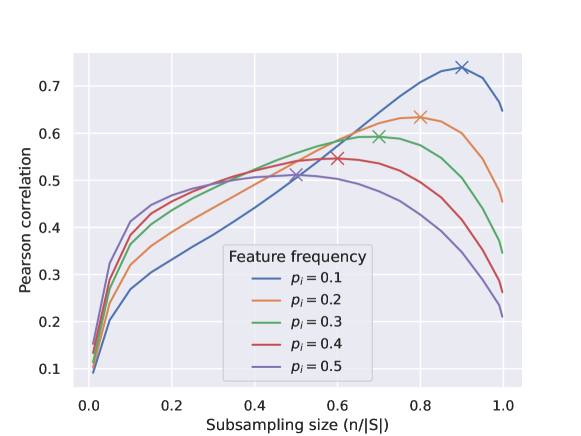
Appendix C Selecting Output Function to Model
In this section, we outline a heuristic method for selecting the output function to model. The heuristic is neither sufficient nor necessary for least-squares regression to work, but may provide some signal as to which output may yield better datamodels.
The first problem we would like to avoid is “output saturation,” i.e., being unable to learn a good datamodel due to insufficient variation in the output. This effect is most pronounced when we measure model correctness: indeed, over 30% of the CIFAR-10 test set is either always correct or always incorrect over all models trained, making datamodel estimation impossible. However, this issue is not unique to correctness. We propose a very simple test inspired by the idealized ordinary least squares model to measure how normally distributed a given type of model output is.
Normally distributed residuals.
In the idealized ordinary least squares model, the observed outputs would follow a normal distribution with fixed mean and unknown variance, where is the true parameter vector. Although we cannot guarantee this condition, we can measure the “normality” of the outputs (again, for a single fixed subset), with the intuition that the more normal the observed outputs are, the better a least-squares regression will work. Hence, compare different output functions by estimating the noise distribution of datamodels given each choice of output function. We leverage our ability—in contrast to typical settings for regression— to sample multiple response variables for a fixed (by retraining several models on the same data and recording the output on a fixed test example).
In Figure 17, we show the results of normality test for residuals arising from different choices of : correctness function, confidence on the correct class, cross-entropy loss, and finally correct-class margin141414Correct-class margin is the difference between the correct-class logit and the highest incorrect-class logit; it is unbounded by definition, and its sign indicates the correctness of the classification.. Correct-class margins is the only choice of where the -values are distributed nearly uniformly, which is consistent with the outputs being normally distributed. Hence, we choose to use the correct-class margins as the dependent variable for fitting our datamodels.

Appendix D Experimental Setup
D.1 Datasets
CIFAR-10.
We use the standard CIFAR-10 dataset [Kri09a].
FMoW.
FMoW [CFW+18a] is a land use classification dataset based on satellite imagery. WILDS [KSM+20a] uses a subset of FMoW and repurposes it as a benchmark for out-of-distribution (OOD) generalization; we use same the variant (presized to 224x224, single RGB image per example rather than a time sequence). We perform our analysis only on the in-distribution train/test splits (e.g. overlapping years) as our focus is not on OOD settings. Also, we limit our data to the year 2012. (These restrictions are only for convenience, and our framework can easily extend and scale to more general settings.)
Properties of both datasets are summarized in Table 2.
| Dataset | Classes | Size (Train/Test) | Input Dimensions |
| CIFAR-10 | 10 | 50,000/10,000 | |
| FMoW | 62 | 21,404/3,138 |
D.2 Models and hyperparameters
CIFAR-10.
We use a ResNet-9 variant from Kakao Brain151515https://github.com/wbaek/torchskeleton/blob/master/bin/dawnbench/cifar10.py optimized for fast training. The hyperparameters (Table 3) were chosen using a grid search. We use the standard batch SGD. For data augmentation, we use random 4px random crop with reflection padding, random horizontal flip, and CutOut [DT17a].
FMoW.
We use the standard ResNet-18 architecture [HZR+16a]. The hyperparameters (Table 3) were chosen using a grid search, including over different optimizers (SGD, Adam) and learning rate schedules (step decay, cyclic, reduce on plateau). As in [KSM+20a], we do not use any data augmentation. Unlike prior work, we do not initialize from a pre-trained ImageNet model; while this results in lower accuracy, this allows us to focus on the role of the FMoW dataset in isolation.
| Dataset | Initial LR | Batch Size | Epochs | Cyclic LR Peak Epoch | Momentum | Weight Decay |
| CIFAR-10 | 0.5 | 512 | 24 | 5 | 0.9 | 5e-4 |
| FMoW | 0.4 | 512 | 15 | 6 | 0.9 | 1e-3 |
Performance.
In Table 4, we show for each dataset the accuracies of the chosen model class (with its specific hyperparameters), across different values of .
| Accuracy (%) | ||
| Subset size () | CIFAR-10 | FMoW |
| 1.0 | 93.00 | 33.76 |
| 0.75 | 91.77 | 31.16 |
| 0.5 | 89.61 | 25.97 |
| 0.2 | 81.62 | 14.70 |
| 0.1 | 71.60 | N/A |
D.3 Training infrastructure
Computing resources.
We train our models on a cluster of machines, each with 9 NVIDIA A100 GPUs and 96 CPU cores. We also use half-precision to increase training speed.
Data loading.
We use FFCV [LIE+22a], which removes the data loading bottleneck for smaller models and allows us achieve a throughput of over 5,000 CIFAR-10 models a day per GPU.
Data processing.
Our datamodel estimation uses (the characteristic vectors) of training subsets and model outputs (margins) on train and test sets. Hence, we do not need to store any model checkpoints, as it suffices to store the training subset and the model outputs after evaluating at the end of training. In particular, training subsets and model outputs can be stored as or matrices, with one row for each model instance and one column for each train or test example. All subsequent computations only require the above matrices.
Appendix E Regression
E.1 Solver details
As mentioned in Section 2, we construct datamodels by running -regularized linear regression, predicting correct-class margins from characteristic vectors, or masks, . The resulting optimization problem is rather large: for example, estimating datamodels for requires running LASSO with a covariate matrix of size , which corresponds to about 60GB of data; for , datamodels this increases five folds as there are 1.5 million models. Moreover, we need to solve up to regression problems (one datamodel each train / test example). The large-scale nature of our estimation problem rules out off-the-shelf solutions such as scikit-learn [PVG+11a], GLMNet [FHT10a], or Celer [MGS18a], all of which either runs out of memory or does not terminate within reasonable time.
Note that solving large linear systems efficiently is an area of active research ([MT20a]), and as a result we anticipate that datamodel estimation could be significantly improved by applying techniques from numerical optimization. In this paper, however, we take a rather simple approach based on the SAGA algorithm of [GGS19a]. Our starting point is the GPU-enabled implementation of [WSM21a]—while this implementation terminated (unlike the CPU-based off-the-shelf solutions), the regressions are still prohibitively slow (i.e., on the order of several GPU-hours per single datamodel estimation). To address this, we make the following changes:
Fast dataloading.
The first performance bottleneck turns out to be in dataloading. More specifically, SAGA is a minibatch-based algorithm: at each iteration, we have to read masks (50,000-dimensional binary vectors) and outputs (scalars) and move them onto the GPU for processing. If the masks are read from disk, I/O speed becomes a major bottleneck—on the other hand, if we pre-load the entire set of masks into memory, then we are not able to run multiple regressions on the same machine, since each regression will use essentially the entire RAM disk. To resolve this issue, we use the FFCV library [LIE+22a] for dataloading—FFCV is based on memory mapping, and thus allows for multiple processes to read from the same memory (combining the benefits of the two aforementioned approaches). FFCV also supports batch pre-loading and parallelization of the data processing pipeline out-of-the-box—adapting the SAGA solver to use FFCV cut the runtime significantly.
Simultaneous outputs.
Next, we leverage the fact that the SAGA algorithm is trivially parallelizable across different instances (sharing the same input matrix), allowing us to estimate multiple datamodels at the same time. In particular, we estimate datamodels for the entire test set in one pass, effectively cutting the runtime of the algorithm by the test set size (e.g., 10,000 for CIFAR-10).
Optimizations.
In order to parallelize across test examples, we need to significantly reduce the GPU memory footprint of the SAGA solver. We accomplish this through a combination of simple code optimization (e.g., using in-place operations rather than copies) as well as writing a few custom CUDA kernels to speed up and reduce the memory consumption of algorithms such as soft thresholding or gradient updating.
Experimental details.
For each dataset considered, we chose a maximum : for CIFAR-10 test, for CIFAR-10 trainset, and for FMoW datamodels. Next, we chose logarithmically spaced intermediate values between as the regularization path. We ran one regression per intermediate , using samples (where is as in the table in Figure 1 (right)) to estimate the parameters of the model and the remaining samples as a validation set. For each image in the test set, we select the corresponding to the best-performing predictor (on the heldout set) along the regularization path. We then re-run the regression once more using these optimal values and the full set of samples.
E.2 Omitted results
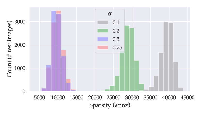


Appendix F Counterfactual Prediction with Datamodels
F.1 General setup
Sample selection.
For all of our counterfactual experiments, we use a random sample of the respective test datasets. We select at random 300 test images for CIFAR-10 (class-balanced; 30 per class) and 100 test images for FMoW. For the CIFAR-10 baselines, we consider counterfactuals for a 100 image subset of the 300.
Size of counterfactuals.
For CIFAR-10, we remove top images and bottom where applicable. For FMoW, we remove top and bottom .
Reducing noise by averaging.
Each counterfactual (i.e., training models on a given training set ) is evaluated over trials to reduce the variance that arises purely from non-determinism in model training. We use for CIFAR-10 and FMoW, and for CIFAR-10 baselines. In Section F.6, we show that using sufficiently high is important for reducing noise.
Control values.
To calculate the actual effects in all of our counterfactual evaluation, we need control values for the “null,” i.e, margins when trained on 100% of the data. We estimate this by averaging over models on trained on the full training set (10,000 for CIFAR-10 and 500 for FMoW).
F.2 Baselines
We describe the baseline methods used to generate data support estimates and counterfactuals. Each of the methods gives a way to select training examples that are most similar or influential to a target example. As in prior work [HYH+21a, PJW+21a], we consider a representative set of baselines spanning both methods based on representation similarity and gradient-based methods, such as influence functions.
Representation distance.
We use distances in the penultimate layer’s representation to rank the training examples in order of similarity to the target test example. We also evaluated dot product, cosine, and mahalanobis distances, but they did not show much variation in their counterfactual effects.161616With the exception of dot product, which performs poorly due to lack of normalization; this is consistent with the findings in [HYH+21a].
In order to more fairly compare with datamodels—so that we can disentangle the variance reduction from using many models and the additional signal captured by datamodels—we also averaged up to 1000 models’ representation distances171717We simply average the ranks from each model, but there are potentially better ways to aggregate them., but this had no discernible difference on the size of the counterfactual effects.
Influence functions.
We apply the influence function approximation introduced in [KL17a]. In particular, we use the following first-order approximation for the influence of on the loss evaluated at :
where is the empirical risk minimizer on the training set and is the Hessian of the loss. The influence here is just the dot product of gradients, weighted by the Hessian. We approximate these influence values by using the methods in [KL17a] and as implemented (independently) in pytorch-influence-functions.181818https://github.com/nimarb/pytorch_influence_functions As in [KL17a], we take a pretrained representation (of a ResNet-9 model, same as that modeled by our datamodels), and compute approximate influence functions with respect to only the parameters in the last linear layer.
TracIn.
[PLS+20a] define an alternative notion of influence: the influence of a training example on a test example is the total change in loss on contributed by updates from mini-batches containing —intuitively, this measures whether gradient updates from are helpful to learning example . They approximate this in practice with TracInCP, which considers checkpoints across training, and sums the dot product of the gradients at and at each checkpoint:
One can view TracInCP as a variant of the gradient dot product, but averaged over models at different epochs) and weighted by the learning rate .
Random baseline.
We also consider a random baseline of removing examples from the same class.
F.3 Data support estimation
Setup.
We use datamodels together with counterfactual evaluations in a guided search to efficiently estimate upper bounds on the size of data supports. For a given target example with corresponding datamodel , we want to find candidate training subsets of small size whose removal most reduces the classification margin on :
| (18) |
Because is a linear model in our case, the solution to the above minimization problem is simply the set corresponding to the largest coordinates of the datamodel parameter :
| (19) |
Our goal is to the find the smallest of these subsets so that , i.e., the example is misclassified on average as per our definition.191919Note that does not imply that the probability of misclassification is greater than 50%. Nonetheless, it is a natural threshold. Thus, for each target , we try several values of , , , , , , , , training models on the set and evaluating the resulting models on .202020While a binary search over for each would be more sample efficient, we collect the entire grid of samples for simplicity. We train models on each counterfactual to reduce variance.
(Given that we are using datamodels as surrogates after all, one might wonder if the above counterfactual evaluations are actually necessary—one could instead consider estimating the optimal directly from . We revisit a heuristic estimation procedure based on this idea at the end of this subsection.)
Estimation methodology.
We assume that the expected margin after removing examples decreases monotonically in ; this is expected from the linearity of our datamodels and is further supported empirically (see Figure 22). Then, our goal is to estimate the unique zero212121More precisely, the upper ceiling as data support is defined as an integer quantity. of the above function based on (noisy) samples of at our chosen values of . Note that by definition, is an upper bound on . Now, because of our monotonicity assumption, we can cast estimating as instance of an isotonic regression problem [RWD88a]); this effectively performs piecewise linear interpolation, while ensuring that monotonicity constraint is not violated. We use sklearn’s IsotonicRegression to fit an estimate , and use this to estimate .

Verifying support estimates.
Due to stochasticity in evaluating counterfactuals, the estimate is noisy. Thus, it is possible that is not a valid upper bound on , e.g. removing top examples do not misclassify . In fact, removing and re-training shows that only 67% of the images are actually misclassified. To establish an upper bound on that has sufficient coverage, we evaluate the counterfactuals after removing an additional 20% of highest datamodel weights, e.g. removing top examples for each test example. When an additional 20% of training examples are removed, 92% of test examples are misclassified. Hence, we use for our final estimates of .
F.3.1 Estimation using baselines
As baselines, we use the same guided search algorithm described above, but instead of using datamodel-predicted values to guide the search, we select the candidate subset using each of the baselines methods described in Section F.2. In particular, we choose the candidate subset for a given as follows:
-
1.
Representation distance: top closest training examples to as measured by distance in the representation space of a pre-trained ResNet-9.
-
2.
Influence estimates (influence functions and TracIn): top training examples with highest (most positive) estimated influence on the target example :
-
3.
Random: first examples from a random ordering222222The random ordering is fixed across different choices of , but not across different targets. of training examples from the same class as .
F.3.2 Heuristic estimates for data support
While we constructively estimate the data supports by training models on counterfactuals and using the above estimation procedure, we can also consider a simpler and cheaper heuristic to estimate assuming the fidelity of the linear datamodels: compute the smallest s.t. the sum of the highest datamodel weights for exceeds the average margin of . In Figure 24, we compare the predicted data supports based on this heuristic to the estimated ones from earlier, and find that they are highly correlated. In practice, this can be a more efficient alternative to quantify brittleness without additional model training (beyond the initial ones to estimate the datamodels).
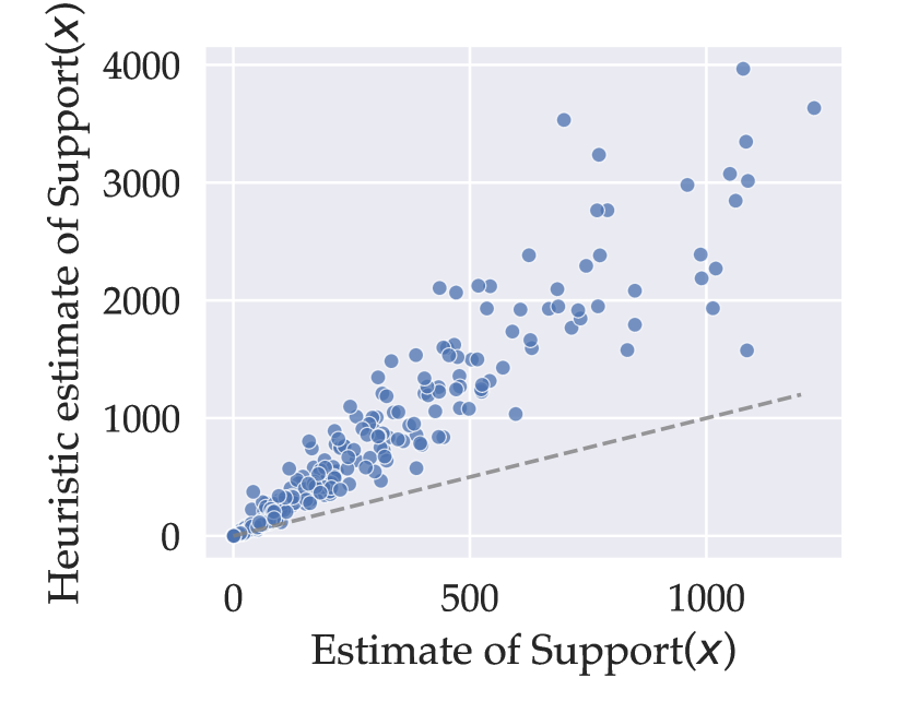
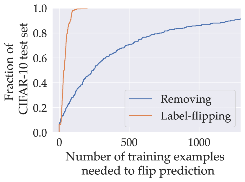
F.4 Brittleness to mislabeling
To study the brittleness of model predictions to mislabeling training images, we take the same 300 random CIFAR-10 test examples and analyze them as follows: First, we find for each example the incorrect class with the highest average logit (across 10,000 models trained on the full training set). Then, we construct counterfactual datasets similarly as in Section F.3 where we take the top training examples with the highest datamodel weights, but this time mislabel them with the incorrect class identified earlier. After training models on each counterfactual, for each target example we estimate the number of mislabeled examples at which the expected margin becomes zero, using the same estimation procedure described in Section F.3. The resulting mislabeling brittleness estimates are shown in Figure 24.
F.5 Comparing raw effect sizes
Instead of comparing the data support estimates (which are derived quantities), here we directly compare the average counterfactual effect (i.e. delta margins) of groups selected using different methods. Figure 25 shows again that datamodels identify much larger effects. Among baselines, we see that TracIn performs best, followed by representation distance. We also see that the representation baseline does not gain any additional signal from simple averaging over models.

F.6 Effect of training stochasticity
As described in Section F.1, we re-train up to models for each counterfactual to reduce noise that arises solely from stochasticity of model training. These additional samples significantly reduces unexplained variance: Figure 27 shows the reduction in variance (“thickness” in the -direction) and the resulting increase in correlation as the number of re-training runs is increased from to .
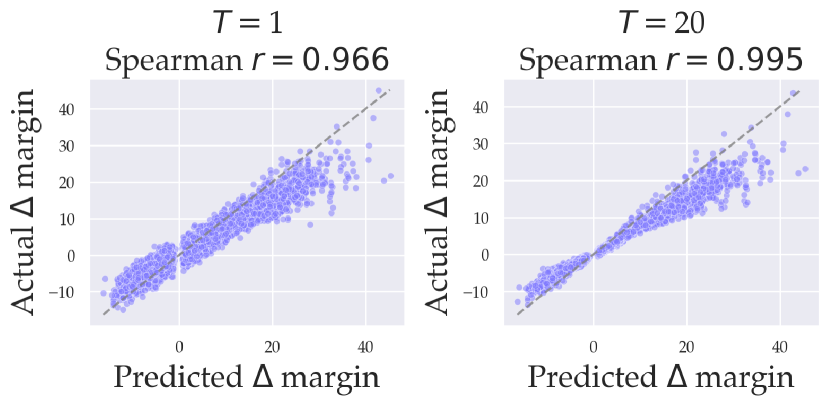
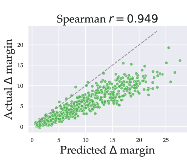
F.7 Transfer to different architecture
While the main premise of datamodeling is understanding how data is used by a given fixed learning algorithm, it is natural to ask how well datamodels can predict across different learning algorithms. We expect some degradation in predictiveness, as datamodels are fit to a particular learning algorithm; at the same time, we also expect some transfer of predictive power as modern deep neural networks are known to make similar predictions and errors [MMS+19a, TSC+19a].
Here, we study one of the factors in a learning algorithm, the choice of architecture. We take the same counterfactuals and evaluate them on ResNet-18 models, using the same training hyperparameters. As expected, the original datamodels continue to predict accurate counterfactuals for the new model class but with some degradation (Figure 27).
F.8 Stress testing
Section 4.1 showed that datamodels excel at predicting counterfactuals across a variety of removal mechanisms. In an effort to find cases where datamodel predictions are not predictive of data counterfactuals, we evaluate the following additional counterfactuals:
-
•
Larger groups of examples (up to 20% of the dataset): we remove 2560, 5120, 10240 top weights using different datamodels . The changes in margin have more unexplained variance when larger number of images are removed; nonetheless, the overall correlation remains high ((Figure 28)).
-
•
Groups of training examples whose predicted effects are zero: we remove 20, 40, 80, 160, 320, 640, 1280, 2560 examples with zero weight (), chosen randomly among all such examples. All of tested counterfactuals had negligible impact on the actual margin, consistent with the prediction of datamodels (Figure 29(a)).
-
•
Groups of examples whose predicted effect is negative according to baselines: we test TracIn and influence functions. (We do not consider the representation distance baseline here is there is no obvious way of extracting this information from it.) Correlation degrades but remains high (Figure 29(b)). Note that the relative scale of the effects is much smaller compared to counterfactuals generated using datamodels (Figure 29(a)).
In general, although there is some reduction in datamodels’ predictiveness, we nevertheless find that datamodels continue to be accurate predictors of data counterfactuals.

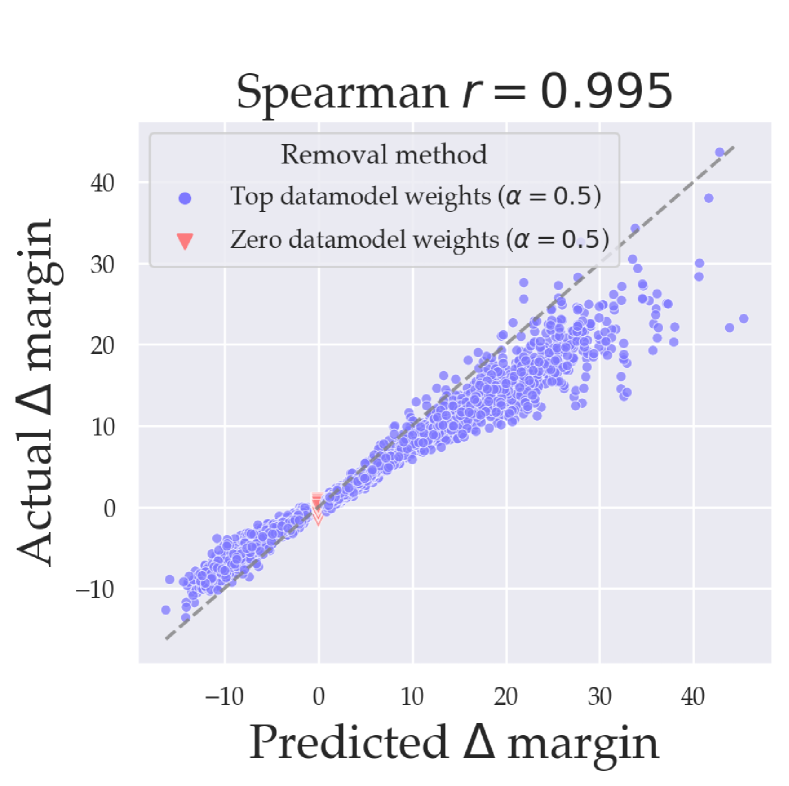
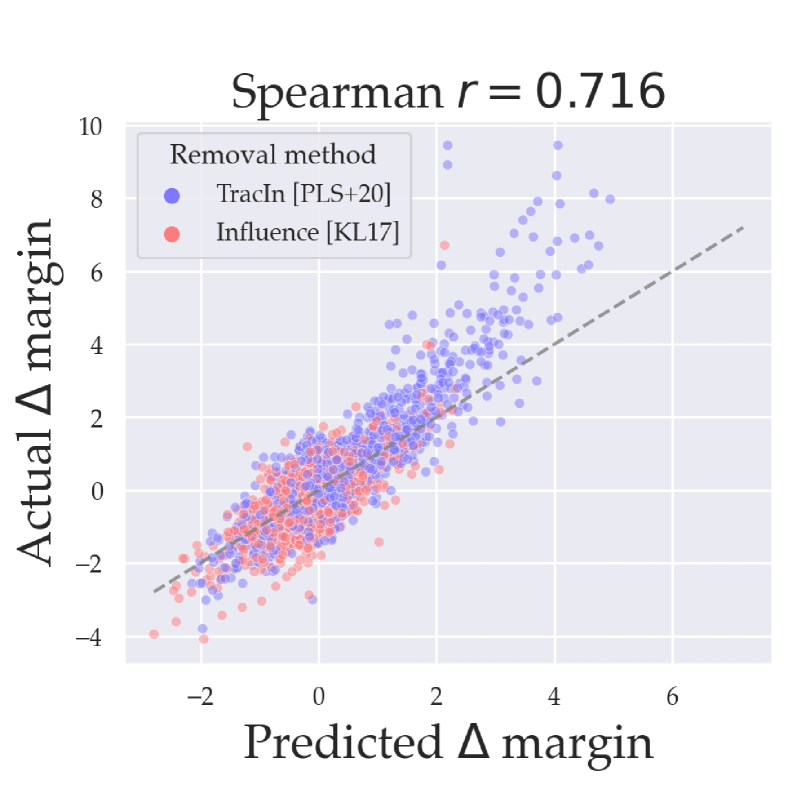
Counterfactuals relative to a random control.
All of the counterfactuals studied so far are relative a fixed control (the entire training set). Here, we consider counterfactuals relative to a random control at (i.e. ). The motivation for considering the shifted control is two folds: first, the counterfactuals generated relative to such are closer in distribution to the original distribution to which datamodels were fit to, so it is natural to study datamodels in this regime; second, this tests whether the counterfactual predictability is robust to the exact choice of the trainset. Latter is desirable, as ultimately we would like to understand how models behave on training sets similar in distribution to , not the exact train set.
To implement above, after removing a target group from the full train set , we subsample the remainder with probability . We adjust the control values accordingly to , where is the subsampling distribution. The results show that one can indeed also predict counterfactuals relative a random control (Figure 30).
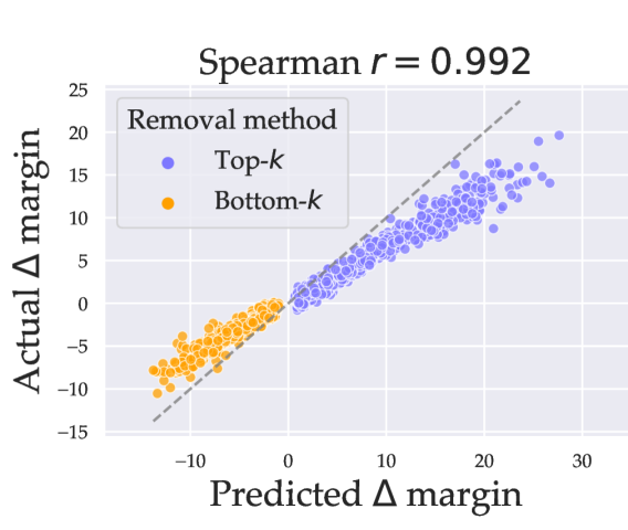
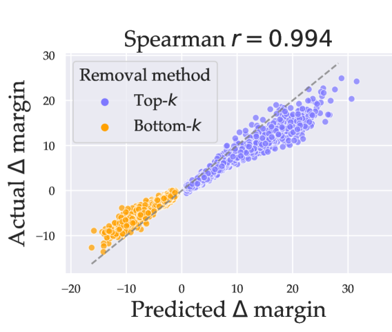
F.9 Additional plots for different values
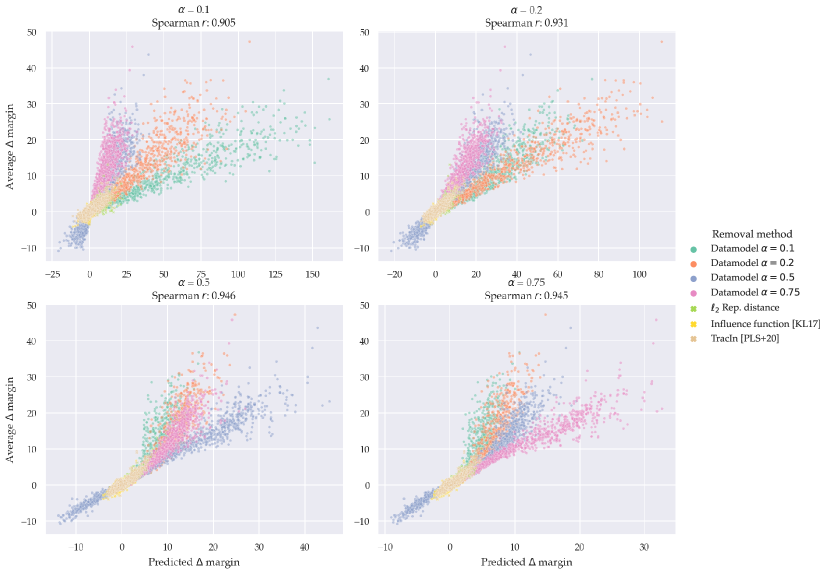

Appendix G Nearest Neighbors
In this section we show additional examples of held-out images and their corresponding train image, datamodel weight pairs.
G.1 CIFAR
In Figure 33 we show more randomly selected test images along with their positive and negative weight training examples. In Figure 34 we show more examples of test images and their corresponding top train images as we vary . In Figure 35 we compare most similar images to given test images identified using various baselines (see Section F.2 for their description).
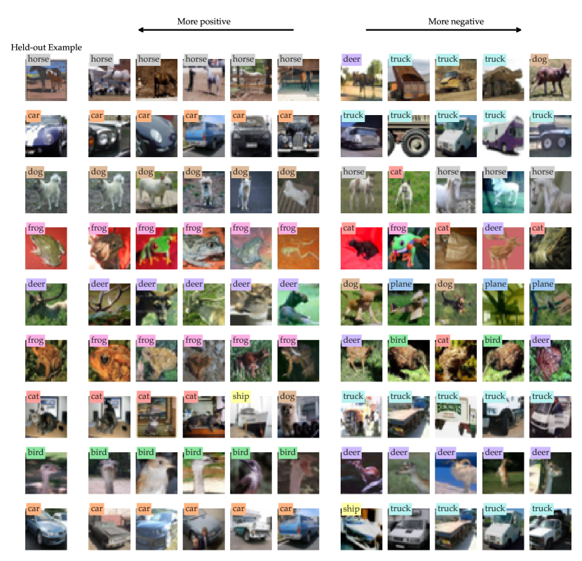
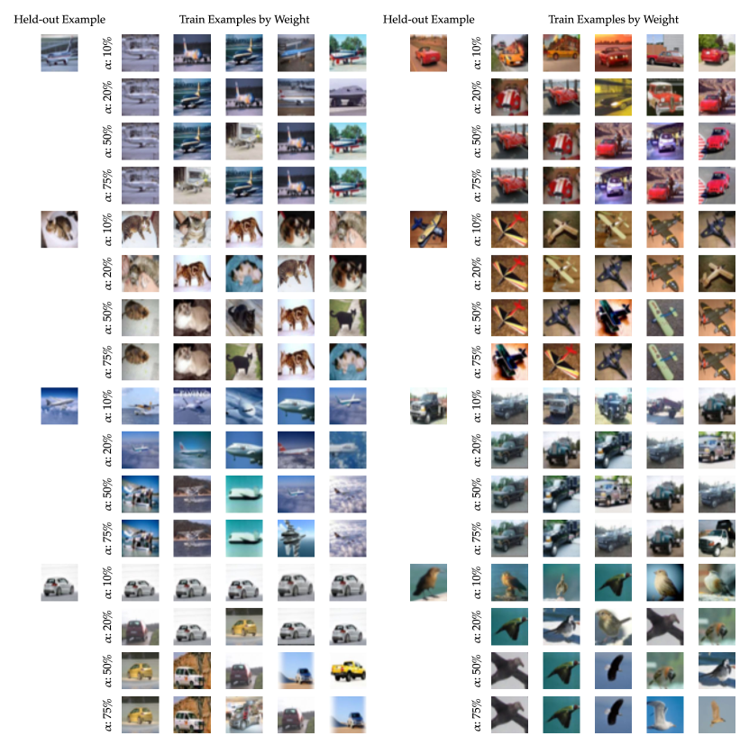
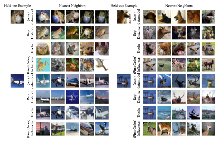
G.2 FMoW
In Figure 36 we show randomly selected target images along with their top-weight train images, using datamodels of different . In Figure 37 we show more examples of test images and their corresponding top train images as we vary .

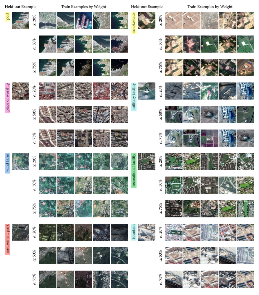
Appendix H Train-Test Leakage
H.1 CIFAR
Task setup.
The general setup is as described Section 4.2.2. In the Amazon Mechanical Turk interface (Figure 38), for each test image we displayed the top 5 and bottom 5 train examples by datamodel weight; the vast majority of potential leakage found corresponded to the top 5 examples. Nine different workers filled out each task. We paid 12 cents per task completed and used these qualifications: locale in US/CA/GB and percentage of hits approved .

Examples.
Figure 39 shows more examples of (train, test) pairs stratified by annotation score. While there is no ground truth due to lack of metadata, we see that the crowdsourced annotation combined with high quality candidates (as identified by datamodels) can effectively surface leaked examples.
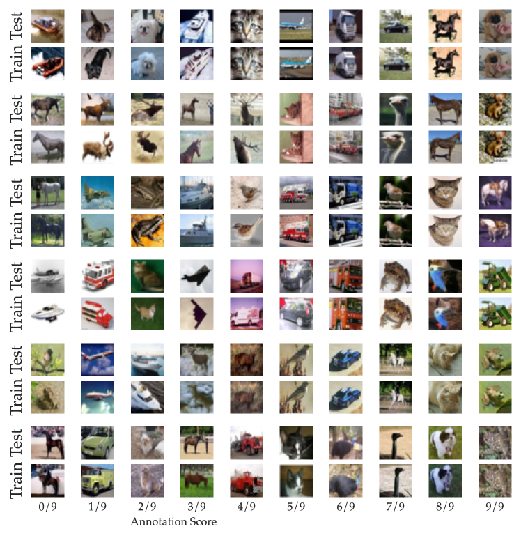
Comparison with CIFAIR.
[BD20a] present CIFAIR, a version of CIFAR with fewer duplicates. The authors define duplicates slightly differently than our definition of same scene train-test leakage (cf. Section 3.2 of their work and our interface shown in Figure 38). They identify train-test leakage by using a deep neural network to measure representation space distances between images across training partitions and manually inspecting the lowest distances.
H.2 FMoW
Appendix Figure 40 shows the CDF of each test image’s minimum distance to a train image.
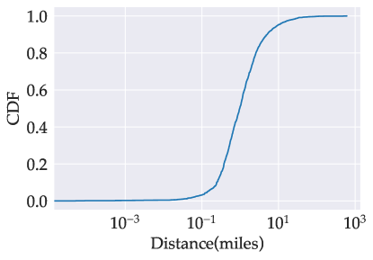
Appendix I Spectral Clustering
I.1 Method
We use sklearn’s cluster.SpectralClustering. Internally, this computes similarity scores using the radial basis function (RBF) kernel on the datamodel embeddings. Then, it runs spectral clustering on the graph defined by the similarity matrix : it computes a Laplacian , represents each node using the first eigenvectors of , and runs -means clustering on the resulting feature representations. We use .
I.2 Omitted results
Figure 41 compares top clusters for the horse class across different . Figure 42 shows additional clusters for eight other classes, apart from the ones shown in Figure 13.
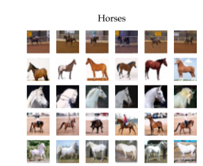
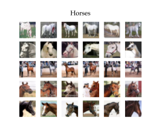
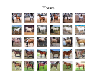
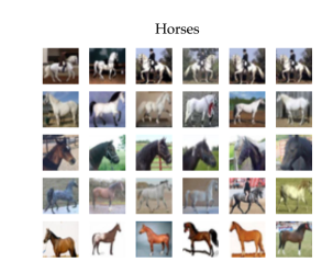
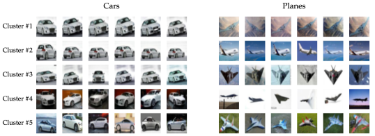
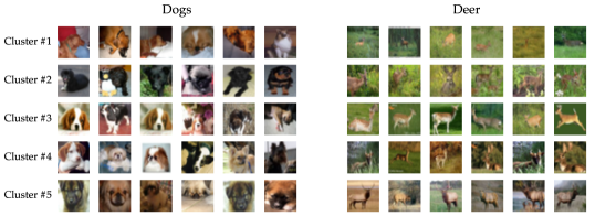
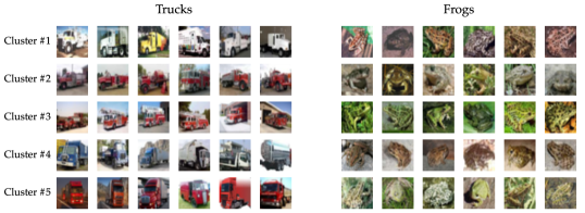
Appendix J PCA on Datamodel Embeddings
J.1 CIFAR
Setup.
For the PCA experiments, we use datamodels for the training and test sets estimated with unless mentioned otherwise.
Effective dimensionality.
In Figure 43, we compare the effective dimensionality of datamodel embeddings with that of a deep representation pretrained on CIFAR-10.
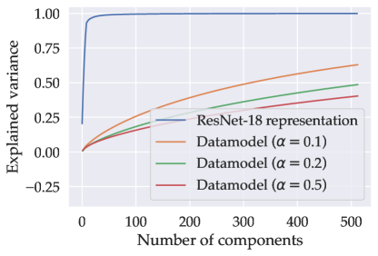
Analyzing model-faithfulness.
To see whether PCA directions reflect model behavior, we look at how “removing” different principal components affect model predictions. More precisely, we remove training examples corresponding to:
-
•
Top most positive coordinates of the principal component vector
-
•
Top most negative coordinates of the principal component vector
Then, for each principal component direction considered, we measure their impact on three groups of held-out samples:
-
•
The top 100 examples by most positive projection on the principal component
-
•
The bottom 100 examples by most negative projection on the principal component
-
•
The full test set
For each of these groups, we measure the mean change in margin after removing different principal component directions. Our results (Figure 44) show that:
-
•
Removing the most positive coordinates of the PC decreases margin on the test set examples with the most positive projections on the PC and increases margin on the examples with the most negative projections on the PC.
-
•
Removing the most negative coordinates of the PC has the opposite effect, increasing margin on the positive projection examples and decreasing margin on the negative projection examples.
-
•
Increasing the size of each removed set increases the effect magnitude.
-
•
Removing PC’s have negligible impact on the aggregate test set, indicating that the impact of different PC’s are roughly “orthogonal,” as one would expect based on the orthogonality of the PCs.
- •
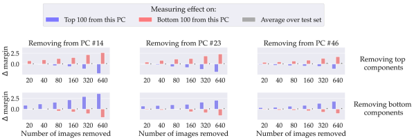
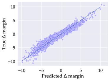
Representation baseline.
In Figure 46 we show the top principal components computed using a representation embedding.
Additional results.
In Figure 47 we show additional PCs from a datamodel PCA.
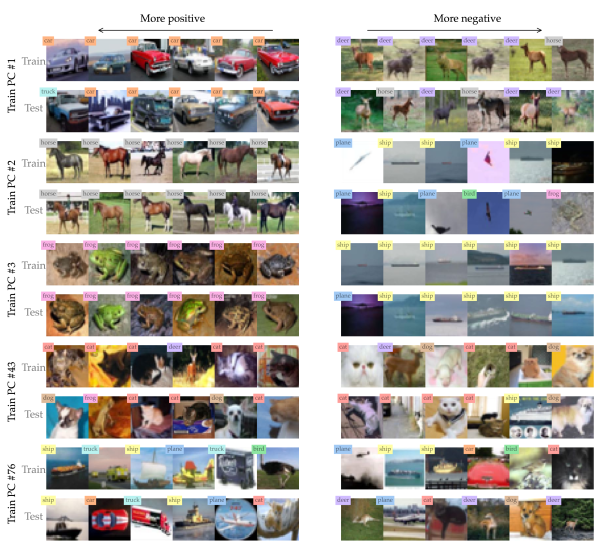
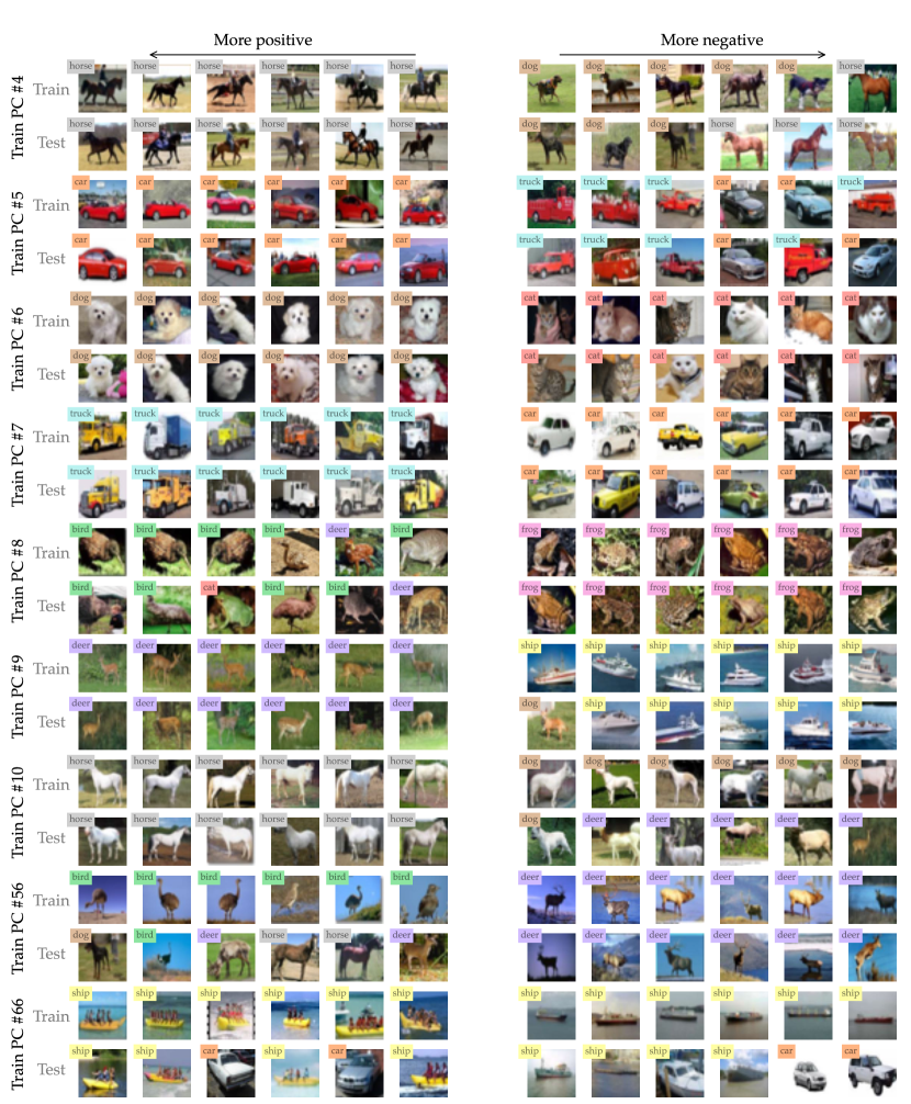
J.2 FMoW
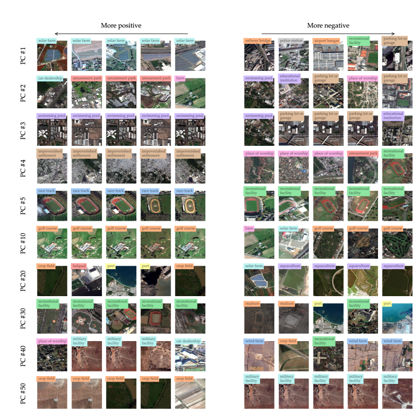
Appendix K Connection between Influence Estimation and Datamodels
K.1 Proof of Lemma 6.1
*
Proof.
For convenience, we introduce the binary mask matrix such that is an indicator for whether the -th training image was included in . Note that is a random matrix with fixed row sum of . Next, we define the output vector that indicates whether a model trained on was correct on . Finally, we introduce the count matrix , i.e., a diagonal matrix whose entries are the columns sums of , e.g. the number of times each example appears across different masks.
We begin with . Consider the matrix . The diagonal entries of this matrix are (due to having constant row sum), while the off-diagonal is
Since has bounded entries (), we have that for fixed , , and in particular
Now, using the Sherman-Morrison formula,
By construction, the row sums of are , and so . Thus,
We now shift our attention to the empirical influence estimator . Using our notation, we can rewrite the (vectorized) empirical influence estimator (15) as:
Now, as for fixed , the random variable converges to with probability . Thus,
and the empirical influence estimator , which completes the proof. ∎
K.2 Evaluating influence estimates as datamodels
Lemma 6.1 suggests that we can re-cast empirical influence estimates as (rescaled) datamodels fit with least-squares loss. Under this view, (i.e., ignoring the difference in conceptual goal), we can differentiate between explicit datamodels and those arising from empirical influences along three axes:
-
•
Estimation algorithm: Most importantly, datamodels explicitly minimize the squared error between true and predicted model outputs. Furthermore, datamodels as instantiated here use (a) a sparsity prior and (b) a bias term which may help generalization.
-
•
Scale: Driven by their intended applications (where one typically only needs to estimate the highest-influence training points for a given test point), empirical influence estimates are typically computed with relatively few samples (i.e., , in our setting) [FZ20a]. In contrast, we find that for datamodel loss to plateau, one needs to estimate parameters using a much larger set of models.
-
•
Output type: Finally, datamodels do not restrict to prediction of a binary correctness variable—in this paper, for example, for deep classification models we find that correct-class margin was best both heuristically and in practice.
In this section, we thus ask: how well do the rescaled datamodels that arise from empirical influence estimates predict model outputs? We address this question in the context of the three axes of variation described above. In order to make results comparable across different outputs types (e.g., correctness vs. correct-class margin), we measure correlation (in the sense of [Spe04a]) between the predicted and true model outputs, in addition to MSE where appropriate. To ensure a conservative comparison, we also measure performance as a predictor of correctness. In particular, we treat as a continuous predictor of the binary variable , and compute the AUC of this predictor (intuitively, this should favor empirical influence estimates since they are computed using correctnesses directly).
In Table 5 we show the difference between empirical influence estimates (first row) and our final datamodel estimates (last row), while disentangling the effect of the three axes above using the rows in between. As expected, there is a vast difference in terms of correlation between the original empirical influence estimates and explicit datamodels.
| Algorithm | # models () | Output type | Spearman | MSE | AUC | Difference |
| Diff. of means | 25,000 | Correctness | 0.028 | N/A | 0.529 | |
| Diff. of means | 100,000 | Correctness | 0.053 | N/A | 0.555 | Under Over-determined |
| Diff. of means | 100,000 | Margin | 0.213 | 2.052 | 0.653 | Output type |
| LASSO | 100,000 | Margin | 0.320 | 1.382 | 0.724 | Explicit datamodel |
We further illustrate this point in Figure 49, where we show how the correlation, MSE, and AUC vary with for both empirical influence estimates and datamodels, as well as an intermediate estimator that uses the estimation procedure of empirical influence estimates but replaces correctness with margin.
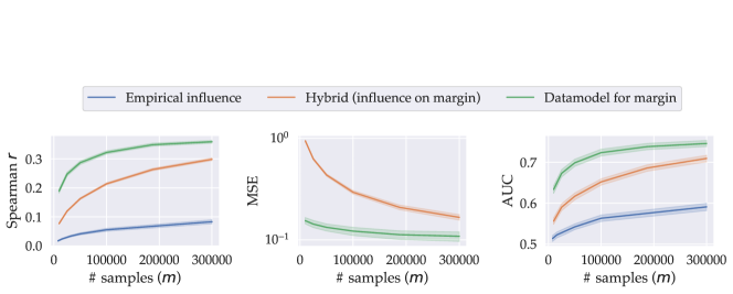
K.3 Testing Lemma 6.1 empirically
In this section, we visualize the performance of empirical influence estimates ([FZ20a]) as datamodels. In Figures 50(a) and 50(b) we plot the distributions of for different CIFAR-10 test examples; Figure 50(a) shows these “conditional prediction distributions” for subsets that were used to estimate the empirical influence, while Figure 50(b) shows the corresponding distributions on held-out (unseen) subsets . The figures suggest that (i) indeed, empirical influences are somewhat predictive of the correctness , (ii) their predictiveness increases as number of samples but is still rather low, and (c) a significant amount of the prediction error is generalization error, as the train predictions in Figure 50(a) are significantly better-separated than the heldout predictions in Figure 50(b).
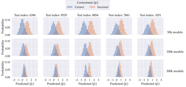
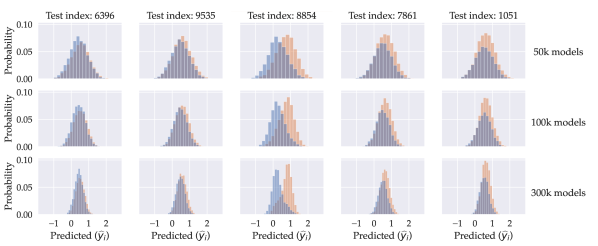
K.4 View of empirical influences as a Taylor approximation
Section 6.1 shows that we can interpret empirical influences as (rescaled) estimates of the weights of a linear datamodel. Here, we give an alternative intuition for why this is the case, even though the definition of empirical influence does not explicitly assume linearity anywhere: we show that the influences define a first-order Taylor approximation of the multilinear extension of our target function of interest, where the influences (approximately) correspond to first-order derivatives of .
Recall that we want to learn some output of interest , say the probability of correctness on a test example , as a function of the examples included in the training set. We first extend this function continuously so that we can take its derivatives. The multilinear extension [Owe72a] of set function to the domain () is given by:
| (20) |
also has an intuitive interpretation: it is the expected value of when is chosen by including each in the input with probability .
Next, we take the derivative of w.r.t. to the input :
Note that because is multilinear, the derivative w.r.t. to is constant in , but not w.r.t. to other . Now, observe that the above expression evaluated at corresponds approximately232323There are two sources of approximation here. First, the -subsampling used in our datamodel definition is defined globally (e.g. fraction of entire train set), which is different from the i.i.d. sampling that is considered here. Second, we only observe noisy versions of . to -subsampled influence , of on : the first term corresponds (using our earlier interpretation) to the expectation of conditional on including , and the second to that conditional on excluding .
Finally, the first-order Taylor approximation of around an is given as:
where are the empirical influences.
The role of .
The above perspective provides an alternative way to think the role of the sampling fraction . The weights depend on the regime we are interested in; if we use -subsampled influences, then we are effectively taking a local linear approximation of in the regime around .
Remark.
Though we include the exposition above for completeness, this is a classical derivation that has appeared in similar form in prior works [Owe72a]. Another connection is that Shapley value is equivalent to the integral of along the “main diagonal” of the hypercube; it is effectively empirical influences averaged uniformly over the choice of .
