Stochastic 2D Signal Generative Model with Wavelet Packets Basis Regarded as a Random Variable and Bayes Optimal Processing thanks: This work was supported by JSPS KAKENHI Grant Numbers JP17K06446 and JP19K04914

Ryohei Oka Dept. Pure and Applied Mathematics
Waseda University
Okubo, Shinjuku-ku, Tokyo, Japan
ryohei1207@toki.waseda.jp
   Yuta Nakahara Center for Data Science
Waseda University
Nishiwaseda, Shinjuku-ku, Tokyo, Japan
yuta.nakahara@aoni.waseda.jp
   Toshiyasu Matsushima Dept. Pure and Applied Mathematics
Waseda University
Okubo, Shinjuku-ku, Tokyo, Japan
toshimat@waseda.jp
Abstract

This study deals with two-dimensional (2D) signal processing using the wavelet packet transform. When the basis is unknown the candidate of basis increases in exponential order with respect to the signal size. Previous studies do not consider the basis as a random variable. Therefore, the cost function needs to be used to select a basis. However, this method is often a heuristic and a greedy search because it is impossible to search all the candidates for a huge number of bases. Therefore, it is difficult to evaluate the entire signal processing under a criterion, and also it does not always guarantee the optimality of the entire signal processing. In this study, we propose a stochastic generative model in which the basis is regarded as a random variable. This makes it possible to evaluate entire signal processing under a unified criterion i.e. Bayes criterion. Moreover, we can derive an optimal signal processing scheme that achieves the theoretical limit. This derived scheme shows that all the bases should be combined according to the posterior instead of selecting a single basis. Although exponential order calculations are required for this scheme, we have derived a recursive algorithm for this scheme, which successfully reduces the computational complexity from the exponential order to the polynomial order.

Index Terms:
Bayesian decision theory, stochastic generative model, wavelet packets

I Introduction

This study deals with two-dimensional (2D) signal processing using the wavelet packet transform. Specifically, We perform 2D signal processing based on statistical decision theory (see e.g. [1]) with Bayes risk function as the evaluation criterion.

Wavelet packet transform has been applied in various fields, and a lot of research has been done in recent years. For example, denoising (see e.g. [2, 3]), compression (see e.g. [4]) , classification (see e.g. [5]), and so on. In any case, they have difficulty in finding an optimal basis because the candidate of basis increases in exponential order with respect to the size of the signal.

Most previous studies do not consider the basis as a random variable. Therefore, some cost functions, for example, such as Shannon entropy [2], need to be used to search and select a basis. However, this method is often a heuristic and a greedy search because it is impossible to search all the candidates for a huge number of bases. Therefore, it is difficult to evaluate the entire signal processing under a criterion, and also it does not always guarantee the optimality of the entire signal processing.

In this study, we propose a stochastic generative model in which the basis is regarded as a random variable. In other words, we consider Bayesian modeling of the basis. This makes it possible to evaluate entire signal processing under a criterion called Bayes risk function in the framework of statistical decision theory[1]. Moreover, we can derive an optimal signal processing scheme that achieves the theoretical limit by using well-known theorems in the framework of statistical decision theory. In the derived scheme, all the bases are weighted by the posterior probability. This shows that any single basis should not be chosen under the Bayes criterion.

In this study, we use this stochastic generative model for denoising. However, there is a problem with the scheme that achieves the theoretical limit. The problem is that the amount of computation increases exponentially with respect to the size of the signal. To solve this problem, we have derived a recursive algorithm that utilizes the property of prior distribution assumed for the basis. This algorithm successfully reduces the computational complexity from the exponential order to the polynomial order without loss of optimality.

In section IV we conduct two numerical experiments about the derived algorithm. The first is an experiment on the posterior distribution of the basis. In this experiment, we confirm that the posterior probability of the true basis is high. The second is an experiment to see the value of Bayes risk function. In this experiment, we compare the value of the Bayes risk function of the proposed method with that of the denoising method under some fixed wavelet packet bases to confirm the effectiveness of the proposed methods.

II Proposed model

In this section, we define Walsh wavelet packets basis (see e.g. [6]) and propose a stochastic model. In the following, we assume the 2D signal size is L×L=2dmax×2dmax(dmax{0})𝐿𝐿superscript2subscript𝑑superscript2subscript𝑑subscript𝑑0L\times L=2^{d_{\max}}\times 2^{d_{\max}}(d_{\max}\in\mathbb{N}\cup\{0\}).

II-A 2D wavelet packets [6]

Definition 1

(wi,j(n)subscript𝑤𝑖𝑗𝑛w_{i,j}(n))
The function wi,j::subscript𝑤𝑖𝑗w_{i,j}:\mathbb{Z}\to\mathbb{R} is defined as follows.

w0,0(n)subscript𝑤00𝑛\displaystyle w_{0,0}(n) {1(n=0)0(otherwise),absentcases1𝑛00otherwise\displaystyle\coloneqq\begin{cases}1&(n=0)\\ 0&(\text{otherwise}),\end{cases} (1)
wi+1,2j(n)subscript𝑤𝑖12𝑗𝑛\displaystyle w_{i+1,2j}(n) 21/2wi,j(n)+21/2wi,j(n2i),absentsuperscript212subscript𝑤𝑖𝑗𝑛superscript212subscript𝑤𝑖𝑗𝑛superscript2𝑖\displaystyle\coloneqq 2^{-1/2}w_{i,j}(n)+2^{-1/2}w_{i,j}(n-2^{i}), (2)
wi+1,2j+1(n)subscript𝑤𝑖12𝑗1𝑛\displaystyle w_{i+1,2j+1}(n) 21/2wi,j(n)21/2wi,j(n2i),absentsuperscript212subscript𝑤𝑖𝑗𝑛superscript212subscript𝑤𝑖𝑗𝑛superscript2𝑖\displaystyle\coloneqq 2^{-1/2}w_{i,j}(n)-2^{-1/2}w_{i,j}(n-2^{i}), (3)

where i{0,1,,dmax}𝑖01subscript𝑑i\in\{0,1,\cdots,d_{\max}\} and j{0,1,,2i1}𝑗01superscript2𝑖1j\in\{0,1,\cdots,2^{i}-1\}.

Definition 2

(wi,j0,j1(n0,n1)subscript𝑤𝑖subscript𝑗0subscript𝑗1subscript𝑛0subscript𝑛1w_{i,j_{0},j_{1}}(n_{0},n_{1}))
The function wi,j0,j1:×:subscript𝑤𝑖subscript𝑗0subscript𝑗1w_{i,j_{0},j_{1}}:\mathbb{Z}\times\mathbb{Z}\to\mathbb{R} is defined as follows.

wi,j0,j1(n0,n1)subscript𝑤𝑖subscript𝑗0subscript𝑗1subscript𝑛0subscript𝑛1\displaystyle w_{i,j_{0},j_{1}}(n_{0},n_{1}) wi,j0(n0)wi,j1(n1),absentsubscript𝑤𝑖subscript𝑗0subscript𝑛0subscript𝑤𝑖subscript𝑗1subscript𝑛1\displaystyle\coloneqq w_{i,j_{0}}(n_{0})w_{i,j_{1}}(n_{1}), (4)

where i{0,1,,dmax}𝑖01subscript𝑑i\in\{0,1,\cdots,d_{\max}\} and j0,j1{0,1,,2i1}.subscript𝑗0subscript𝑗101superscript2𝑖1j_{0},j_{1}\in\{0,1,\cdots,2^{i}-1\}.

Definition 3

(Wi,j0,j1,k0,k1subscript𝑊𝑖subscript𝑗0subscript𝑗1subscript𝑘0subscript𝑘1W_{i,j_{0},j_{1},k_{0},k_{1}})
The matrix Wi,j0,j1.k0,k1L×Lsubscript𝑊formulae-sequence𝑖subscript𝑗0subscript𝑗1subscript𝑘0subscript𝑘1superscript𝐿𝐿W_{i,j_{0},j_{1}.k_{0},k_{1}}\in\mathbb{R}^{L\times L} is defined as follows.

Wi,j0,j1,k0,k1subscript𝑊𝑖subscript𝑗0subscript𝑗1subscript𝑘0subscript𝑘1\displaystyle W_{i,j_{0},j_{1},k_{0},k_{1}}
(wi,j0,j1(n02ik0,n12ik1))n0,n1{0,1,,L},absentsubscriptsubscript𝑤𝑖subscript𝑗0subscript𝑗1subscript𝑛0superscript2𝑖subscript𝑘0subscript𝑛1superscript2𝑖subscript𝑘1subscript𝑛0subscript𝑛101𝐿\displaystyle\coloneqq(w_{i,j_{0},j_{1}}(n_{0}-2^{i}k_{0},n_{1}-2^{i}k_{1}))_{n_{0},n_{1}\in\{0,1,\cdots,L\}}, (5)

where k0,k1{0,1,,L/2i1}.subscript𝑘0subscript𝑘101𝐿superscript2𝑖1k_{0},k_{1}\in\{0,1,\cdots,L/2^{i}-1\}.

Definition 4

(𝒲i,j0,j1L×Lsubscript𝒲𝑖subscript𝑗0subscript𝑗1superscript𝐿𝐿\mathcal{W}_{i,j_{0},j_{1}}\subseteq\mathbb{R}^{L\times L})
Let 𝒲i,j0,j1L×Lsubscript𝒲𝑖subscript𝑗0subscript𝑗1superscript𝐿𝐿\mathcal{W}_{i,j_{0},j_{1}}\subseteq\mathbb{R}^{L\times L} be the space of 2D signals that consist of a linear combination of {Wi,j0,j1,k0,k1}k0,k1{0,1,,L/2i1}subscriptsubscript𝑊𝑖subscript𝑗0subscript𝑗1subscript𝑘0subscript𝑘1subscript𝑘0subscript𝑘101𝐿superscript2𝑖1\{W_{i,j_{0},j_{1},k_{0},k_{1}}\}_{k_{0},k_{1}\in\{0,1,\cdots,L/2^{i}-1\}}.

Definition 5

(𝐰i,j0,j1,k0,k1subscript𝐰𝑖subscript𝑗0subscript𝑗1subscript𝑘0subscript𝑘1\bm{w}_{i,j_{0},j_{1},k_{0},k_{1}})
Let 𝐰i,j0,j1,k0,k1subscript𝐰𝑖subscript𝑗0subscript𝑗1subscript𝑘0subscript𝑘1\bm{w}_{i,j_{0},j_{1},k_{0},k_{1}} be the vertical vector whose components are those of Wi,j0,j1,k0,k1subscript𝑊𝑖subscript𝑗0subscript𝑗1subscript𝑘0subscript𝑘1W_{i,j_{0},j_{1},k_{0},k_{1}} rearranged in raster scan order.

Under the above definition, the following property holds.

Proposition 1

(𝒲0,0,0subscript𝒲000\mathcal{W}_{0,0,0})
The following relationship holds

𝒲0,0,0subscript𝒲000\displaystyle\mathcal{W}_{0,0,0} =L×L.absentsuperscript𝐿𝐿\displaystyle=\mathbb{R}^{L\times L}. (6)
Proposition 2

(Orthonormal basis of 𝒲i,j0,j1subscript𝒲𝑖subscript𝑗0subscript𝑗1\mathcal{W}_{i,j_{0},j_{1}})
{Wi,j0,j1,k0,k1}k0,k1{0,1,,L/2i1}subscriptsubscript𝑊𝑖subscript𝑗0subscript𝑗1subscript𝑘0subscript𝑘1subscript𝑘0subscript𝑘101𝐿superscript2𝑖1\{W_{i,j_{0},j_{1},k_{0},k_{1}}\}_{k_{0},k_{1}\in\{0,1,\cdots,L/2^{i}-1\}} forms an orthonormal basis for 𝒲i,j0,j1subscript𝒲𝑖subscript𝑗0subscript𝑗1\mathcal{W}_{i,j_{0},j_{1}}.

Proposition 3

(Decomposition of space)
 The following relationship holds.

𝒲i,j0,j1=subscript𝒲𝑖subscript𝑗0subscript𝑗1absent\displaystyle\mathcal{W}_{i,j_{0},j_{1}}= 𝒲i+1,2j0,2j1𝒲i+1,2j0,2j1+1direct-sumsubscript𝒲𝑖12subscript𝑗02subscript𝑗1subscript𝒲𝑖12subscript𝑗02subscript𝑗11\displaystyle\hskip 2.84544pt\mathcal{W}_{i+1,2j_{0},2j_{1}}\oplus\mathcal{W}_{i+1,2j_{0},2j_{1}+1}
𝒲i+1,2j0+1,2j1𝒲i+1,2j0+1,2j1+1.direct-sumdirect-sumsubscript𝒲𝑖12subscript𝑗012subscript𝑗1subscript𝒲𝑖12subscript𝑗012subscript𝑗11\displaystyle\oplus\mathcal{W}_{i+1,2j_{0}+1,2j_{1}}\oplus\mathcal{W}_{i+1,2j_{0}+1,2j_{1}+1}. (7)

Note that direct-sum\oplus denotes the orthogonal direct sum.

From the aforementioned properties, the entire space of 2D signals can be represented as an orthogonal direct sum of subspaces corresponding to the leaf nodes of the full quadtree111All nodes have 4 child nodes or no child node. with 𝒲0,0,0subscript𝒲000\mathcal{W}_{0,0,0} as the root node. The basis of each subspace can be used to construct an orthonormal basis.

Example 1

(Full quadtree)
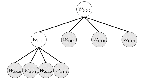
When the relation 𝒲0,0,0=(𝒲2,0,0𝒲2,0,1𝒲2,1,0𝒲2,1,1)𝒲1,0,1𝒲1,1,0𝒲1,1,1subscript𝒲000direct-sumdirect-sumsubscript𝒲200subscript𝒲201subscript𝒲210subscript𝒲211subscript𝒲101subscript𝒲110subscript𝒲111\mathcal{W}_{0,0,0}=(\mathcal{W}_{2,0,0}\oplus\mathcal{W}_{2,0,1}\oplus\mathcal{W}_{2,1,0}\oplus\mathcal{W}_{2,1,1})\oplus\mathcal{W}_{1,0,1}\oplus\mathcal{W}_{1,1,0}\oplus\mathcal{W}_{1,1,1} holds, the diagram of the full quadtree is at Fig. 1. The gray area represents leaf nodes. Notably, the basis of 2D-DWT corresponds to the full quadtree created by extending branches only in the direction j0=j1=0subscript𝑗0subscript𝑗10j_{0}=j_{1}=0.

Refer to caption
Figure 1: example for quadtree under dmax=2subscript𝑑2d_{\max}=2

II-B 2D wavelet packets basis matrix

Definition 6

(𝒮,,,sr𝒮subscript𝑠r\mathcal{S},\mathcal{L},\mathcal{I},s_{\text{r}})
Let 𝒮𝒮\mathcal{S} be the set of nodes in a complete quadtree222All leaf nodes have the same depth. of depth dmaxsubscript𝑑d_{\max} and 𝒮𝒮\mathcal{L}\subset\mathcal{S} be the set of its leaf nodes and 𝒮𝒮\mathcal{I}\subset\mathcal{S} be the set of its inner nodes. Let srsubscript𝑠rs_{\text{r}} be the root node.

Definition 7

(,m,msuperscript𝑚superscript𝑚\mathcal{M},\mathcal{L}^{m},\mathcal{I}^{m})
Let \mathcal{M} be the set of all full quadtrees on 𝒮𝒮\mathcal{S}, which contain srsubscript𝑠rs_{\text{r}} and whose depth is less than or equal to dmaxsubscript𝑑d_{\max}. Let m𝒮superscript𝑚𝒮\mathcal{L}^{m}\subset\mathcal{S} be the set of leaf nodes in m𝑚m\in\mathcal{M} and m𝒮superscript𝑚𝒮\mathcal{I}^{m}\subset\mathcal{S} be the set of inner nodes in m𝑚m\in\mathcal{M}.

Definition 8

(Wmsuperscript𝑊𝑚W^{m})
Let WmL2×L2superscript𝑊𝑚superscriptsuperscript𝐿2superscript𝐿2W^{m}\in\mathbb{R}^{L^{2}\times L^{2}} be a matrix created by collecting the basis of the subspace corresponding to the leaf nodes in m𝑚m\in\mathcal{M}. The matrix WmL2×L2superscript𝑊𝑚superscriptsuperscript𝐿2superscript𝐿2W^{m}\in\mathbb{R}^{L^{2}\times L^{2}} is called the basis matrix in this paper.

Definition 9

(Wssubscript𝑊𝑠W_{s})
Let WsL2×L2subscript𝑊𝑠superscriptsuperscript𝐿2superscript𝐿2W_{s}\in\mathbb{R}^{L^{2}\times L^{2}} be the basis at s𝒮𝑠𝒮s\in\mathcal{S} which is appropriately complemented by 0 vectors so that the following relation holds.

Wmsuperscript𝑊𝑚\displaystyle W^{m} =smWs.absentsubscript𝑠superscript𝑚subscript𝑊𝑠\displaystyle=\sum_{s\in\mathcal{L}^{m}}W_{s}. (8)
Example 2

(The basis matrix corresponding to the quadtree m𝑚m\in\mathcal{M} in Figure 1)

Wmsuperscript𝑊𝑚\displaystyle W^{m} =(𝒘1,0,0,0,0𝒘1,0,0,0,1𝒘1,0,0,1,0𝒘1,0,0,1,1𝟎12×16)+(𝟎4×16𝒘1,0,1,0,0𝒘1,0,1,0,1𝒘1,0,1,1,0𝒘1,0,1,1,1𝟎8×16)+(𝟎8×16𝒘1,1,0,0,0𝒘1,1,0,0,1𝒘1,1,0,1,0𝒘1,1,0,1,1𝟎4×16)absentmatrixsuperscriptsubscript𝒘10000topsuperscriptsubscript𝒘10001topsuperscriptsubscript𝒘10010topsuperscriptsubscript𝒘10011topsubscript01216matrixsubscript0416superscriptsubscript𝒘10100topsuperscriptsubscript𝒘10101topsuperscriptsubscript𝒘10110topsuperscriptsubscript𝒘10111topsubscript0816matrixsubscript0816superscriptsubscript𝒘11000topsuperscriptsubscript𝒘11001topsuperscriptsubscript𝒘11010topsuperscriptsubscript𝒘11011topsubscript0416\displaystyle=\begin{pmatrix}\bm{w}_{1,0,0,0,0}^{\top}\\ \bm{w}_{1,0,0,0,1}^{\top}\\ \bm{w}_{1,0,0,1,0}^{\top}\\ \bm{w}_{1,0,0,1,1}^{\top}\\ \bm{0}_{12\times 16}\end{pmatrix}+\begin{pmatrix}\bm{0}_{4\times 16}\\ \bm{w}_{1,0,1,0,0}^{\top}\\ \bm{w}_{1,0,1,0,1}^{\top}\\ \bm{w}_{1,0,1,1,0}^{\top}\\ \bm{w}_{1,0,1,1,1}^{\top}\\ \bm{0}_{8\times 16}\end{pmatrix}+\begin{pmatrix}\bm{0}_{8\times 16}\\ \bm{w}_{1,1,0,0,0}^{\top}\\ \bm{w}_{1,1,0,0,1}^{\top}\\ \bm{w}_{1,1,0,1,0}^{\top}\\ \bm{w}_{1,1,0,1,1}^{\top}\\ \bm{0}_{4\times 16}\\ \end{pmatrix}
+(𝟎12×16𝒘2,2,2,0,0𝟎3×16)+(𝟎13×16𝒘2,2,3,0,0𝟎2×16)+(𝟎14×16𝒘2,3,2,0,0𝟎1×16)matrixsubscript01216superscriptsubscript𝒘22200topsubscript0316matrixsubscript01316superscriptsubscript𝒘22300topsubscript0216matrixsubscript01416superscriptsubscript𝒘23200topsubscript0116\displaystyle+\begin{pmatrix}\bm{0}_{12\times 16}\\ \bm{w}_{2,2,2,0,0}^{\top}\\ \bm{0}_{3\times 16}\\ \end{pmatrix}+\begin{pmatrix}\bm{0}_{13\times 16}\\ \bm{w}_{2,2,3,0,0}^{\top}\\ \bm{0}_{2\times 16}\\ \end{pmatrix}+\begin{pmatrix}\bm{0}_{14\times 16}\\ \bm{w}_{2,3,2,0,0}^{\top}\\ \bm{0}_{1\times 16}\\ \end{pmatrix}
+(𝟎15×16𝒘2,3,3,0,0).matrixsubscript01516superscriptsubscript𝒘23300top\displaystyle+\begin{pmatrix}\bm{0}_{15\times 16}\\ \bm{w}_{2,3,3,0,0}^{\top}\\ \end{pmatrix}. (9)

where 𝟎k×lsubscript0𝑘𝑙\bm{0}_{k\times l} is a k×l𝑘𝑙k\times l zero matrix.

The basis matrix Wmsuperscript𝑊𝑚W^{m} is orthonormal because it consists of an orthonormal basis.

II-C Stochastic generative model

Herein, we describe the stochastic 2D signal model.

Definition 10

(𝐗,𝐱𝐗𝐱\bm{X},\bm{x})
Let 𝐗𝐗\bm{X} be a random variable vector on L2×1superscriptsuperscript𝐿21\mathbb{R}^{L^{2}\times 1} representing 2D signal and 𝐱L2×1𝐱superscriptsuperscript𝐿21\bm{x}\in\mathbb{R}^{L^{2}\times 1} be its realization. 𝐱L2×1𝐱superscriptsuperscript𝐿21\bm{x}\in\mathbb{R}^{L^{2}\times 1} is a vertical vector that is given by sorting L×L𝐿𝐿L\times L size 2D signal in raster scan order. 2D-DWPT 𝛉𝛉\bm{\theta} defined below also has a similar structure.

Definition 11

(𝛉𝛉\bm{\theta})
Let 𝛉𝛉\bm{\theta} be a random variable vector on L2×1superscriptsuperscript𝐿21\mathbb{R}^{L^{2}\times 1} representing the 2D-DWPT. Its realization is similarly written as 𝛉L2×1𝛉superscriptsuperscript𝐿21\bm{\theta}\in\mathbb{R}^{L^{2}\times 1}.

The following relationship holds between 𝒙𝒙\bm{x} and 𝜽𝜽\bm{\theta}.

𝜽𝜽\displaystyle\bm{\theta} =Wm𝒙,absentsuperscript𝑊𝑚𝒙\displaystyle=W^{m}\bm{x}, (10)
𝒙𝒙\displaystyle\ \bm{x} =(Wm)𝜽.absentsuperscriptsuperscript𝑊𝑚top𝜽\displaystyle=(W^{m})^{\top}\bm{\theta}. (11)

In our model, the quadtree m𝑚m\in\mathcal{M} and 2D-DWPT 𝜽𝜽\bm{\theta} are generated by assumed prior distributions, and the 2D signal 𝒙𝒙\bm{x} is generated by a linear transformation of 𝜽𝜽\bm{\theta}.

III Application to Bayesian signal processing

Under the generative probability model discussed in the previous section, various signal processing problems can be considered depending on how the input signal is observed and the nature of the desired output signal. In the Bayesian decision theory[1], these are represented by designing the domain and the range of decision function as well as the loss function. In this section, we formulate the simplest denoising problem based on the Bayesian decision theory and find the optimal denoising under the Bayesian criterion.

III-A Problem

The following additive noises are considered in this paper.

Assumption 1

(additive noise)

𝒀𝑿+ϵ.𝒀𝑿bold-italic-ϵ\displaystyle\bm{Y}\coloneqq\bm{X}+\bm{\epsilon}. (12)

We assume 𝐘𝐘\bm{Y} is a vector of random variables on L2×1superscriptsuperscript𝐿21\mathbb{R}^{L^{2}\times 1} representing the noisy 2D signal, 𝐗𝐗\bm{X} is a random variable representing the original 2D signal, and ϵ𝒩(ϵ|𝟎L2×1,σϵ2I)similar-tobold-ϵ𝒩conditionalbold-ϵsubscript0superscript𝐿21subscriptsuperscript𝜎2bold-ϵ𝐼\bm{\epsilon}\sim\mathcal{N}(\bm{\epsilon}|\bm{0}_{L^{2}\times 1},\sigma^{2}_{\bm{\epsilon}}I) (σϵ2subscriptsuperscript𝜎2bold-ϵ\sigma^{2}_{\bm{\epsilon}}\in\mathbb{R} is a known hyperparameter). In the following, let 𝐲L2×1𝐲superscriptsuperscript𝐿21\bm{y}\in\mathbb{R}^{L^{2}\times 1} be the realization of 𝐘𝐘\bm{Y}. Our goal in Sections III and IV is to estimate 𝐱𝐱\bm{x} from 𝐲𝐲\bm{y}.

We now define the decision function δ𝛿\delta.

Definition 12

(Decision function δ𝛿\delta)
The function δ:L2×1L2×1:𝛿superscriptsuperscript𝐿21superscriptsuperscript𝐿21\delta:\mathbb{R}^{L^{2}\times 1}\to\mathbb{R}^{L^{2}\times 1} is called the decision function. The input of the decision function δ𝛿\delta is the noisy 2D signal 𝐲𝐲\bm{y}, and the output is an estimation for the original 2D signal 𝐱^^𝐱\hat{\bm{x}}.

We define the Bayes optimal decision function δsuperscript𝛿\delta^{\ast} as the function that minimizes the Bayes risk function BR(δ𝛿\delta) based on mean-square error loss in the 2D signal domain.

Definition 13

(Bayes risk function BR(δ)𝐵𝑅𝛿BR(\delta))
 The Bayes risk function BR:Δ:𝐵𝑅ΔBR:\Delta\to\mathbb{R} (ΔΔ\Delta is the space of decision functions δ𝛿\delta) is defined as below.

BR(δ)m𝐵𝑅𝛿subscript𝑚\displaystyle BR(\delta)\coloneqq\sum_{m\in\mathcal{M}}\int\int 1L2𝒙δ(𝒚)21superscript𝐿2superscriptnorm𝒙𝛿𝒚2\displaystyle\frac{1}{L^{2}}\|\bm{x}-\delta(\bm{y})\|^{2}
×p(𝒚|𝒙,m)p(𝒙|m)p(m)d𝒚d𝒙.absent𝑝conditional𝒚𝒙𝑚𝑝conditional𝒙𝑚𝑝𝑚d𝒚d𝒙\displaystyle\times p(\bm{y}|\bm{x},m)p(\bm{x}|m)p(m)\mathrm{d}\bm{y}\mathrm{d}\bm{x}. (13)

III-B Solution to the problem

According to the Bayesian decision theory (see e.g. [1]), the following holds.

Theorem 1

(Bayes optimal decision function δsuperscript𝛿\delta^{\ast})
Bayes optimal decision function δsuperscript𝛿\delta^{\ast} is given by

δ(𝒚)superscript𝛿𝒚\displaystyle\delta^{\ast}(\bm{y}) =mp(m|𝒚)𝒙p(𝒙|m,𝒚)d𝒙.absentsubscript𝑚𝑝conditional𝑚𝒚𝒙𝑝conditional𝒙𝑚𝒚differential-d𝒙\displaystyle=\sum_{m\in\mathcal{M}}p(m|\bm{y})\int\bm{x}p(\bm{x}|m,\bm{y})\mathrm{d}\bm{x}. (14)

There are two problems in the calculation of the right-hand side of the equation (14). First, the integral of 𝒙𝒙\bm{x} does not generally have a closed-form expression. Second, the computation complexity of summation with respect to m𝑚m\in\mathcal{M} increases exponentially with respect to the size of the 2D signal. However, using an appropriate prior distribution of 𝜽𝜽\bm{\theta} and the prior distribution of the quadtree model m𝑚m\in\mathcal{M}, the computational complexity can be reduced to polynomial order while maintaining optimality.

III-C Efficient algorithm for the solution

Let 𝝁mL2×1superscript𝝁𝑚superscriptsuperscript𝐿21\bm{\mu}^{m}\in\mathbb{R}^{L^{2}\times 1} and σ2superscript𝜎2\sigma^{2}\in\mathbb{R} be a known hyperparameters. 𝝁msuperscript𝝁𝑚\bm{\mu}^{m} is constructed in the same way as Wmsuperscript𝑊𝑚W^{m}, where 𝝁m=sm𝝁s(𝝁sL2×1\bm{\mu}^{m}=\sum_{s\in\mathcal{L}^{m}}\bm{\mu}_{s}\hskip 2.84544pt(\bm{\mu}_{s}\in\mathbb{R}^{L^{2}\times 1} is also a known vector).

Assumption 2

(2D-DWPT prior distribution)

p(𝜽|m)𝑝conditional𝜽𝑚\displaystyle p(\bm{\theta}|m) 𝒩(𝜽|𝝁m,σ2I),absent𝒩conditional𝜽superscript𝝁𝑚superscript𝜎2𝐼\displaystyle\coloneqq\mathcal{N}(\bm{\theta}|\bm{\mu}^{m},\sigma^{2}I), (15)

where I𝐼I is the L2×L2superscript𝐿2superscript𝐿2L^{2}\times L^{2} identity matrix.

By linear transformation, we can show that the 2D signal 𝑿𝑿\bm{X} follows the normal distribution as below.

Proposition 4

(Distribution of the 2D signal)
The distribution of the 2D signal 𝐗𝐗\bm{X} is given by

p(𝒙|m)𝑝conditional𝒙𝑚\displaystyle p(\bm{x}|m) =𝒩(𝒙|(Wm)𝝁m,σ2I).absent𝒩conditional𝒙superscriptsuperscript𝑊𝑚topsuperscript𝝁𝑚superscript𝜎2𝐼\displaystyle=\mathcal{N}(\bm{x}|(W^{m})^{\top}\bm{\mu}^{m},\sigma^{2}I). (16)
Assumption 3

(Prior distribution of the quadtree model)

p(m)𝑝𝑚\displaystyle p(m) =sm(1gs)smgsabsentsubscriptproduct𝑠superscript𝑚1subscript𝑔𝑠subscriptproductsuperscript𝑠superscript𝑚subscript𝑔superscript𝑠\displaystyle=\prod_{s\in\mathcal{L}^{m}}(1-g_{s})\prod_{s^{\prime}\in\mathcal{I}^{m}}g_{s^{\prime}} (17)

where gs[0,1]subscript𝑔𝑠01g_{s}\in[0,1] is a known hyperparameter for any s𝒮𝑠𝒮s\in\mathcal{S}, which satisfies gs=0subscript𝑔𝑠0g_{s}=0 for s𝑠s\in\mathcal{L}. The gssubscript𝑔𝑠g_{s} represents the probability that node s𝑠s will extend a branch.

The aforementioned prior distribution (17) was proposed in [7] to represent context trees and applied in [8] to represent the prior distribution of 1D wavelet packets trees. A mathematically rigorous proof of the following equation (18), their expected values, and posterior probability calculations is given in [9].

mp(m)=1subscript𝑚𝑝𝑚1\displaystyle\sum_{m\in\mathcal{M}}p(m)=1 (18)

There has not been any previous study that applied this prior distribution to 2D-DWPT trees to our best knowledge. Hence, we applied this prior distribution to 2D-DWPT trees for the first time.

Under the aforementioned assumptions, the following theorem can be derived.

Theorem 2

(Posterior distribution)
The following equation holds.

p(𝒙|m,𝒚)𝑝conditional𝒙𝑚𝒚\displaystyle p(\bm{x}|m,\bm{y}) =𝒩(𝒙|𝝁~m,σ~2I),absent𝒩conditional𝒙superscript~𝝁𝑚superscript~𝜎2𝐼\displaystyle=\mathcal{N}(\bm{x}|\tilde{\bm{\mu}}^{m},\tilde{\sigma}^{2}I), (19)
p(m|𝒚)𝑝conditional𝑚𝒚\displaystyle p(m|\bm{y}) =sm(1g~s)smg~s,absentsubscriptproduct𝑠superscript𝑚1subscript~𝑔𝑠subscriptproductsuperscript𝑠superscript𝑚subscript~𝑔superscript𝑠\displaystyle=\prod_{s\in\mathcal{L}^{m}}(1-\tilde{g}_{s})\prod_{s^{\prime}\in\mathcal{I}^{m}}\tilde{g}_{s^{\prime}}, (20)

where

𝝁~msuperscript~𝝁𝑚\displaystyle\tilde{\bm{\mu}}^{m} σ2σ2+σϵ2𝒚+σϵ2σ2+σϵ2(Wm)𝝁m,absentsuperscript𝜎2superscript𝜎2subscriptsuperscript𝜎2bold-italic-ϵ𝒚subscriptsuperscript𝜎2bold-italic-ϵsuperscript𝜎2subscriptsuperscript𝜎2bold-italic-ϵsuperscriptsuperscript𝑊𝑚topsuperscript𝝁𝑚\displaystyle\coloneqq\frac{\sigma^{2}}{\sigma^{2}+\sigma^{2}_{\bm{\epsilon}}}\bm{y}+\frac{\sigma^{2}_{\bm{\epsilon}}}{\sigma^{2}+\sigma^{2}_{\bm{\epsilon}}}(W^{m})^{\top}\bm{\mu}^{m}, (21)
σ~2superscript~𝜎2\displaystyle\tilde{\sigma}^{2} σ2σϵ2σ2+σϵ2,absentsuperscript𝜎2subscriptsuperscript𝜎2bold-italic-ϵsuperscript𝜎2subscriptsuperscript𝜎2bold-italic-ϵ\displaystyle\coloneqq\frac{\sigma^{2}\sigma^{2}_{\bm{\epsilon}}}{\sigma^{2}+\sigma^{2}_{\bm{\epsilon}}}, (22)
g~ssubscript~𝑔𝑠\displaystyle\tilde{g}_{s} {gs(s)gssCh(s)ψ~sψ~s(otherwise),absentcasessubscript𝑔𝑠𝑠continued-fractionsubscript𝑔𝑠subscriptproductsuperscript𝑠Ch𝑠subscript~𝜓superscript𝑠subscript~𝜓𝑠otherwise\displaystyle\coloneqq\begin{cases}g_{s}&(s\in\mathcal{L})\\ \cfrac{g_{s}\prod_{s^{\prime}\in\text{Ch}(s)}\tilde{\psi}_{s^{\prime}}}{\tilde{\psi}_{s}}&(\text{otherwise}),\end{cases} (23)
ψ~ssubscript~𝜓𝑠\displaystyle\tilde{\psi}_{s} {ψs(s)(1gs)ψs+gssCh(s)ψ~s(otherwise),absentcasessubscript𝜓𝑠𝑠1subscript𝑔𝑠subscript𝜓𝑠subscript𝑔𝑠subscriptproductsuperscript𝑠Ch𝑠subscript~𝜓superscript𝑠otherwise\displaystyle\coloneqq\begin{cases}\psi_{s}&(s\in\mathcal{L})\\ (1-g_{s})\psi_{s}+g_{s}\prod_{s^{\prime}\in\text{Ch}(s)}\tilde{\psi}_{s^{\prime}}&(\text{otherwise}),\end{cases} (24)
lnψssubscript𝜓𝑠\displaystyle\ln\psi_{s} 1σ2+σϵ2(Ws𝒚𝝁s2)𝝁s.absent1superscript𝜎2subscriptsuperscript𝜎2bold-italic-ϵsuperscriptsubscript𝑊𝑠𝒚subscript𝝁𝑠2topsubscript𝝁𝑠\displaystyle\coloneqq\frac{1}{\sigma^{2}+\sigma^{2}_{\bm{\epsilon}}}\bigg{(}W_{s}\bm{y}-\frac{\bm{\mu}_{s}}{2}\bigg{)}^{\top}\bm{\mu}_{s}. (25)

Note that Ch(s)𝒮Ch𝑠𝒮\text{Ch}(s)\subset\mathcal{S} is the set of child nodes of s𝒮𝑠𝒮s\in\mathcal{S}.

The proof of this theorem is in Appendix A.
Using Theorem 2, the Bayes optimal decision function δsuperscript𝛿\delta^{\ast} can be calculated as follows.

Theorem 3

(Bayes optimal decision function δsuperscript𝛿\delta^{\ast})
The following equation holds

δ(𝒚)superscript𝛿𝒚\displaystyle\delta^{\ast}(\bm{y}) =σ2σ2+σϵ2𝒚+σϵ2σ2+σϵ2mp(m|𝒚)(Wm)𝝁m.absentsuperscript𝜎2superscript𝜎2subscriptsuperscript𝜎2bold-italic-ϵ𝒚subscriptsuperscript𝜎2bold-italic-ϵsuperscript𝜎2subscriptsuperscript𝜎2bold-italic-ϵsubscript𝑚𝑝conditional𝑚𝒚superscriptsuperscript𝑊𝑚topsuperscript𝝁𝑚\displaystyle=\frac{\sigma^{2}}{\sigma^{2}+\sigma^{2}_{\bm{\epsilon}}}\bm{y}+\frac{\sigma^{2}_{\bm{\epsilon}}}{\sigma^{2}+\sigma^{2}_{\bm{\epsilon}}}\sum_{m\in\mathcal{M}}p(m|\bm{y})(W^{m})^{\top}\bm{\mu}^{m}. (26)

The integral of 𝒙𝒙\bm{x} in (14) is solved in (26) but the computational complexity of the second term increases exponentially with the size of the 2D signal. However, using the recursive computation derived from the following theorem, the computational complexity can be reduced to polynomial order while maintaining Bayesian optimality.

Theorem 4

(Recursive algorithm)
The following equation holds.

rsr=mp(m|𝒚)(Wm)𝝁m.subscript𝑟subscript𝑠rsubscript𝑚𝑝conditional𝑚𝒚superscriptsuperscript𝑊𝑚topsuperscript𝝁𝑚\displaystyle r_{s_{\text{r}}}=\sum_{m\in\mathcal{M}}p(m|\bm{y})(W^{m})^{\top}\bm{\mu}^{m}. (27)
rssubscript𝑟𝑠\displaystyle r_{s} {(1g~s)Ws𝝁s(s)(1g~s)Ws𝝁s+g~ssCh(s)rs(otherwise).absentcases1subscript~𝑔𝑠subscriptsuperscript𝑊top𝑠subscript𝝁𝑠𝑠1subscript~𝑔𝑠subscriptsuperscript𝑊top𝑠subscript𝝁𝑠subscript~𝑔𝑠subscriptsuperscript𝑠Ch𝑠subscript𝑟superscript𝑠otherwise\displaystyle\coloneqq\begin{cases}(1-\tilde{g}_{s})W^{\top}_{s}\bm{\mu}_{s}&(s\in\mathcal{L})\\ (1-\tilde{g}_{s})W^{\top}_{s}\bm{\mu}_{s}+\tilde{g}_{s}\sum_{s^{\prime}\in\text{Ch}(s)}r_{s^{\prime}}&(\text{otherwise}).\end{cases} (28)

The proof of this theorem is in Appendix C.

IV Experiments

IV-A Experiment 1 : Posterior p(m|𝐲)𝑝conditional𝑚𝐲p(m|\bm{y})

The purpose of Experiment 1 is to quantitatively confirm that the posterior distribution p(m|𝒚)𝑝conditional𝑚𝒚p(m|\bm{y}) is properly computed.

The setting of Experiment 1 is as follows.

  • dmax=2subscript𝑑2d_{\max}=2.

  • gs=0.5subscript𝑔𝑠0.5g_{s}=0.5.

  • σ2=10superscript𝜎210\sigma^{2}=10.

  • σϵ2=4subscriptsuperscript𝜎2bold-italic-ϵ4\sigma^{2}_{\bm{\epsilon}}=4.

  • 𝝁ssubscript𝝁𝑠\bm{\mu}_{s} is calculated from resized images in [10]. 333Let 𝒙1,,𝒙50000subscript𝒙1subscript𝒙50000\bm{x}_{1},\cdots,\bm{x}_{50000} denote the training images in [10]. Non zero terms of 𝝁ssubscript𝝁𝑠\bm{\mu}_{s} is calculated as 150000×4dmaxi(s)n=150000f(Ws𝒙n)150000superscript4subscript𝑑𝑖𝑠superscriptsubscript𝑛150000𝑓subscript𝑊𝑠subscript𝒙𝑛\frac{1}{50000\times 4^{d_{\max}-i(s)}}\sum_{n=1}^{50000}f(W_{s}\bm{x}_{n}), where f:N:𝑓superscript𝑁f:\mathbb{R}^{N}\to\mathbb{R} is defined as f((a1,a2,,aN))n=1Nan𝑓subscript𝑎1subscript𝑎2subscript𝑎𝑁superscriptsubscript𝑛1𝑁subscript𝑎𝑛f((a_{1},a_{2},\cdots,a_{N}))\coloneqq\sum_{n=1}^{N}a_{n} and i(s)𝑖𝑠i(s) is the depth of node s𝑠s.

This experiment is conducted by using the following procedure.

  1. 1.

    Set m0subscript𝑚0m_{0} (6 in Fig.2).

  2. 2.

    Generate 𝒙p(𝒙|m0)similar-to𝒙𝑝conditional𝒙subscript𝑚0\bm{x}\sim p(\bm{x}|m_{0}).

  3. 3.

    Generate 𝒚=𝒙+ϵ𝒚𝒙bold-italic-ϵ\bm{y}=\bm{x}+\bm{\epsilon}.

  4. 4.

    Calculate g~ssubscript~𝑔𝑠\tilde{g}_{s}.

  5. 5.

    Repeat from step 3 to step 4 50 times.

  6. 6.

    Repeat from step 2 to step 5 50 times.

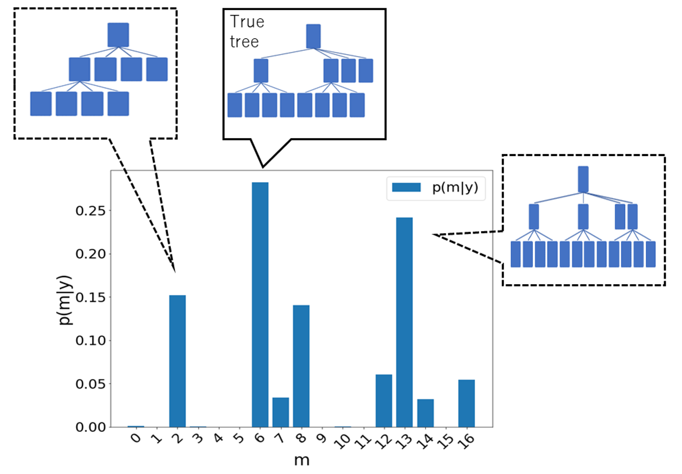
The result of this experiment is in Fig. 2. Since dmax=2subscript𝑑2d_{\max}=2, we have ||=1717|\mathcal{M}|=17. In other words, there are 17 candidate trees in total. we give them indices from 0 to 16 in an arbitrary order. In this experiment, the sixth tree in this order is fixed as the true tree for data generation.
Refer to caption
Figure 2: p(m|𝒚)𝑝conditional𝑚𝒚p(m|\bm{y}) in Experiment 1

According to this result, we can confirm that the posterior probability of the sixth tree, which is the true tree, is the maximum value. Moreover, the tree with only one node expanded from the true tree has the second-largest posterior probability and the tree with only one node shrunk from the true tree has the third-largest posterior probability. Therefore, we confirmed our algorithm properly computed the posterior distribution by not only the theoretical proof but also the quantitative experiment.

IV-B Experiment 2 : Value of Bayes risk function BR(δ)𝐵𝑅𝛿BR(\delta)

The purpose of Experiment 2 is to confirm the effectiveness of the proposed method by calculating the value of the Bayes risk function. We compare the proposed method with the estimated signals from five models mi(i=1,2,3,4,5)subscript𝑚𝑖𝑖12345m_{i}\in\mathcal{M}\hskip 2.84544pt(i=1,2,3,4,5). misubscript𝑚𝑖m_{i} is a perfect quadtree expanded to the depth i𝑖i.

The estimated signals from these models misubscript𝑚𝑖m_{i}\in\mathcal{M} are obtained by the following equations.

δi(𝒚)superscript𝛿𝑖𝒚\displaystyle\delta^{i}(\bm{y}) =σ2σ2+σϵ2𝒚+σϵ2σ2+σϵ2(Wmi)𝝁mi.absentsuperscript𝜎2superscript𝜎2subscriptsuperscript𝜎2bold-italic-ϵ𝒚subscriptsuperscript𝜎2bold-italic-ϵsuperscript𝜎2subscriptsuperscript𝜎2bold-italic-ϵsuperscriptsuperscript𝑊subscript𝑚𝑖topsuperscript𝝁subscript𝑚𝑖\displaystyle=\frac{\sigma^{2}}{\sigma^{2}+\sigma^{2}_{\bm{\epsilon}}}\bm{y}+\frac{\sigma^{2}_{\bm{\epsilon}}}{\sigma^{2}+\sigma^{2}_{\bm{\epsilon}}}(W^{m_{i}})^{\top}\bm{\mu}^{m_{i}}. (29)

The setting of Experiment 2 is as follows.

  • dmax=5subscript𝑑5d_{\max}=5.

  • σ2=10superscript𝜎210\sigma^{2}=10.

  • σϵ2=4subscriptsuperscript𝜎2bold-italic-ϵ4\sigma^{2}_{\bm{\epsilon}}=4.

  • 𝝁ssubscript𝝁𝑠\bm{\mu}_{s} is calculated from images in [10].

This experiment is conducted by using the following procedure.

  1. 1.

    Set gs{0.1,0.2,0.3,0.4,0.5,0.6,0.7,0.8,0.9}subscript𝑔𝑠0.10.20.30.40.50.60.70.80.9g_{s}\in\{0.1,0.2,0.3,0.4,0.5,0.6,0.7,0.8,0.9\}.

  2. 2.

    Gernerate quadtree mp(m)similar-to𝑚𝑝𝑚m\sim p(m).

  3. 3.

    Generate 𝒙p(𝒙|m)similar-to𝒙𝑝conditional𝒙𝑚\bm{x}\sim p(\bm{x}|m).

  4. 4.

    Generate 𝒚=𝒙+ϵ𝒚𝒙bold-italic-ϵ\bm{y}=\bm{x}+\bm{\epsilon}.

  5. 5.

    Calculate δ(𝒚),δi(𝒚)superscript𝛿𝒚superscript𝛿𝑖𝒚\delta^{\ast}(\bm{y}),\delta^{i}(\bm{y}).

  6. 6.

    Calculate mean-square error loss.

  7. 7.

    Repeat from step 4 to step 6 10 times.

  8. 8.

    Repeat from step 3 to step 7 10 times.

  9. 9.

    Repeat from step 2 to step 8 30 times.

Refer to caption
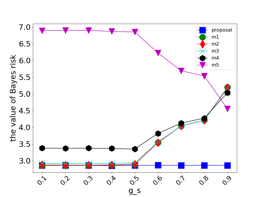
Figure 3: Value of Bayes risk function BR(δ)𝐵𝑅𝛿BR(\delta) for each method
TABLE I: Average depth of m𝑚m\in\mathcal{M} for each gssubscript𝑔𝑠g_{s}
gssubscript𝑔𝑠g_{s} Average depth of m𝑚m\in\mathcal{M}
0.10.10.1 0.000
0.20.20.2 0.290
0.30.30.3 0.957
0.40.40.4 0.897
0.50.50.5 2.318
0.60.60.6 3.243
0.70.70.7 3.974
0.80.80.8 3.732
0.90.90.9 4.452

The result of this experiment is at Fig. 3, and TABLE I shows the average depth444The average depth is calculated as 1|m|smi(s)1superscript𝑚subscript𝑠superscript𝑚𝑖𝑠\frac{1}{|\mathcal{L}^{m}|}\sum_{s\in\mathcal{L}^{m}}i(s).of m𝑚m\in\mathcal{M} for each gssubscript𝑔𝑠g_{s}.

According to this result, we can confirm that the proposed method achieved the minimum value of the Bayes risk function for all noise variances. Moreover, each of δisuperscript𝛿𝑖\delta^{i} depends on the depth of the m𝑚m\in\mathcal{M}. For example, the deeper the average depth of the generated trees is, the higher the value of the Bayes risk function of δ1,δ2,δ3,δ4superscript𝛿1superscript𝛿2superscript𝛿3superscript𝛿4\delta^{1},\delta^{2},\delta^{3},\delta^{4} is, and vice versa. Therefore, we can confirm the effectiveness of the proposed method.

Acknowledgment

The author would like to thank my family for supporting me in my daily life and the members of the Matsushima laboratory for their meaningful discussions.

Appendix A Proof of Theory 2

In the following, let C𝐶C\in\mathbb{R} be a constant. First, we show the equation (19).

lnp(𝒙|m,𝒚)𝑝conditional𝒙𝑚𝒚\displaystyle\ln p(\bm{x}|m,\bm{y}) (30)
=\displaystyle= lnp(𝒚|𝒙,m)+lnp(𝒙|m)+C𝑝conditional𝒚𝒙𝑚𝑝conditional𝒙𝑚𝐶\displaystyle\ln p(\bm{y}|\bm{x},m)+\ln p(\bm{x}|m)+C (31)
=\displaystyle= ln𝒩(𝒚|𝒙,σϵ2I)+ln𝒩(𝒙|(Wm)𝝁m,σ2I)+C𝒩conditional𝒚𝒙subscriptsuperscript𝜎2bold-italic-ϵ𝐼𝒩conditional𝒙superscriptsuperscript𝑊𝑚topsuperscript𝝁𝑚superscript𝜎2𝐼𝐶\displaystyle\ln\mathcal{N}(\bm{y}|\bm{x},\sigma^{2}_{\bm{\epsilon}}I)+\ln\mathcal{N}(\bm{x}|(W^{m})^{\top}\bm{\mu}^{m},\sigma^{2}I)+C (32)
=\displaystyle= 12σϵ2(𝒚𝒙)(𝒚𝒙)12subscriptsuperscript𝜎2bold-italic-ϵsuperscript𝒚𝒙top𝒚𝒙\displaystyle-\frac{1}{2\sigma^{2}_{\bm{\epsilon}}}(\bm{y}-\bm{x})^{\top}(\bm{y}-\bm{x})
12σ2(𝒙(Wm)𝝁m)(𝒙(Wm)𝝁m)+C12superscript𝜎2superscript𝒙superscriptsuperscript𝑊𝑚topsuperscript𝝁𝑚top𝒙superscriptsuperscript𝑊𝑚topsuperscript𝝁𝑚𝐶\displaystyle-\frac{1}{2\sigma^{2}}(\bm{x}-(W^{m})^{\top}\bm{\mu}^{m})^{\top}(\bm{x}-(W^{m})^{\top}\bm{\mu}^{m})+C (33)
=\displaystyle= 12(1σ2+1σϵ2)𝒙𝒙121superscript𝜎21subscriptsuperscript𝜎2bold-italic-ϵsuperscript𝒙top𝒙\displaystyle-\frac{1}{2}\bigg{(}\frac{1}{\sigma^{2}}+\frac{1}{\sigma^{2}_{\bm{\epsilon}}}\bigg{)}\bm{x}^{\top}\bm{x}
+(1σϵ2𝒚+1σ2(Wm)𝝁m)𝒙+C.superscript1subscriptsuperscript𝜎2bold-italic-ϵ𝒚1superscript𝜎2superscriptsuperscript𝑊𝑚topsuperscript𝝁𝑚top𝒙𝐶\displaystyle+\bigg{(}\frac{1}{\sigma^{2}_{\bm{\epsilon}}}\bm{y}+\frac{1}{\sigma^{2}}(W^{m})^{\top}\bm{\mu}^{m}\bigg{)}^{\top}\bm{x}+C. (34)

Let us define σ~2,𝝁~msuperscript~𝜎2superscript~𝝁𝑚\tilde{\sigma}^{2},\tilde{\bm{\mu}}^{m} as follows.

σ~2superscript~𝜎2\displaystyle\tilde{\sigma}^{2} σ2σϵ2σ2+σϵ2,absentsuperscript𝜎2subscriptsuperscript𝜎2bold-italic-ϵsuperscript𝜎2subscriptsuperscript𝜎2bold-italic-ϵ\displaystyle\coloneqq\frac{\sigma^{2}\sigma^{2}_{\bm{\epsilon}}}{\sigma^{2}+\sigma^{2}_{\bm{\epsilon}}}, (35)
𝝁~msuperscript~𝝁𝑚\displaystyle\tilde{\bm{\mu}}^{m} σ~2(1σϵ2𝒚+1σ2(Wm)𝝁m).absentsuperscript~𝜎21subscriptsuperscript𝜎2bold-italic-ϵ𝒚1superscript𝜎2superscriptsuperscript𝑊𝑚topsuperscript𝝁𝑚\displaystyle\coloneqq\tilde{\sigma}^{2}\bigg{(}\frac{1}{\sigma^{2}_{\bm{\epsilon}}}\bm{y}+\frac{1}{\sigma^{2}}(W^{m})^{\top}\bm{\mu}^{m}\bigg{)}. (36)

Therefore,

lnp(𝒙|m,𝒚)𝑝conditional𝒙𝑚𝒚\displaystyle\ln p(\bm{x}|m,\bm{y}) (37)
=\displaystyle= 12σ~2(𝒙𝝁~m)(𝒙𝝁~m)+C12superscript~𝜎2superscript𝒙superscript~𝝁𝑚top𝒙superscript~𝝁𝑚𝐶\displaystyle-\frac{1}{2\tilde{\sigma}^{2}}(\bm{x}-\tilde{\bm{\mu}}^{m})^{\top}(\bm{x}-\tilde{\bm{\mu}}^{m})+C (38)
=\displaystyle= ln𝒩(𝒙|𝝁~m,σ~2I).𝒩conditional𝒙superscript~𝝁𝑚superscript~𝜎2𝐼\displaystyle\ln\mathcal{N}(\bm{x}|\tilde{\bm{\mu}}^{m},\tilde{\sigma}^{2}I). (39)

Next, we show the equation (20).

lnp(m|𝒚)𝑝conditional𝑚𝒚\displaystyle\ln p(m|\bm{y}) (40)
=\displaystyle= lnp(𝒚|m)+lnp(m)+C𝑝conditional𝒚𝑚𝑝𝑚𝐶\displaystyle\ln p(\bm{y}|m)+\ln p(m)+C (41)
=\displaystyle= lnp(𝒚|𝒙,m)p(𝒙|m)d𝒙+lnp(m)+C𝑝conditional𝒚𝒙𝑚𝑝conditional𝒙𝑚differential-d𝒙𝑝𝑚𝐶\displaystyle\ln\int p(\bm{y}|\bm{x},m)p(\bm{x}|m)\mathrm{d}\bm{x}+\ln p(m)+C (42)
=\displaystyle= ln𝒩(𝒚|𝒙,σϵ2I)𝒩(𝒙|(Wm)𝝁m,σ2I)d𝒙𝒩conditional𝒚𝒙subscriptsuperscript𝜎2bold-italic-ϵ𝐼𝒩conditional𝒙superscriptsuperscript𝑊𝑚topsuperscript𝝁𝑚superscript𝜎2𝐼differential-d𝒙\displaystyle\ln\int\mathcal{N}(\bm{y}|\bm{x},\sigma^{2}_{\bm{\epsilon}}I)\mathcal{N}(\bm{x}|(W^{m})^{\top}\bm{\mu}^{m},\sigma^{2}I)\mathrm{d}\bm{x}
+lnp(m)+C𝑝𝑚𝐶\displaystyle+\ln p(m)+C (43)
=\displaystyle= ln𝒩(𝒚|(Wm)𝝁m,(σ2+σϵ2)I)+lnp(m)+C𝒩conditional𝒚superscriptsuperscript𝑊𝑚topsuperscript𝝁𝑚superscript𝜎2subscriptsuperscript𝜎2bold-italic-ϵ𝐼𝑝𝑚𝐶\displaystyle\ln\mathcal{N}(\bm{y}|(W^{m})^{\top}\bm{\mu}^{m},(\sigma^{2}+\sigma^{2}_{\bm{\epsilon}})I)+\ln p(m)+C (44)
=\displaystyle= 12(σ2+σϵ2)(𝒚(Wm)𝝁m)(𝒚(Wm)𝝁m)12superscript𝜎2subscriptsuperscript𝜎2bold-italic-ϵsuperscript𝒚superscriptsuperscript𝑊𝑚topsuperscript𝝁𝑚top𝒚superscriptsuperscript𝑊𝑚topsuperscript𝝁𝑚\displaystyle-\frac{1}{2(\sigma^{2}+\sigma^{2}_{\bm{\epsilon}})}(\bm{y}-(W^{m})^{\top}\bm{\mu}^{m})^{\top}(\bm{y}-(W^{m})^{\top}\bm{\mu}^{m})
+lnp(m)+C𝑝𝑚𝐶\displaystyle+\ln p(m)+C (45)
=\displaystyle= 12(σ2+σϵ2)(𝒚𝒚2𝒚(Wm)𝝁m+(𝝁m)𝝁m)12superscript𝜎2subscriptsuperscript𝜎2bold-italic-ϵsuperscript𝒚top𝒚2superscript𝒚topsuperscriptsuperscript𝑊𝑚topsuperscript𝝁𝑚superscriptsuperscript𝝁𝑚topsuperscript𝝁𝑚\displaystyle-\frac{1}{2(\sigma^{2}+\sigma^{2}_{\bm{\epsilon}})}(\bm{y}^{\top}\bm{y}-2\bm{y}^{\top}(W^{m})^{\top}\bm{\mu}^{m}+(\bm{\mu}^{m})^{\top}\bm{\mu}^{m})
+lnp(m)+C𝑝𝑚𝐶\displaystyle+\ln p(m)+C (46)
=\displaystyle= 1(σ2+σϵ2)(Wm𝒚𝝁m2)𝝁m+lnp(m)+C1superscript𝜎2subscriptsuperscript𝜎2bold-italic-ϵsuperscriptsuperscript𝑊𝑚𝒚superscript𝝁𝑚2topsuperscript𝝁𝑚𝑝𝑚𝐶\displaystyle\frac{1}{(\sigma^{2}+\sigma^{2}_{\bm{\epsilon}})}\bigg{(}W^{m}\bm{y}-\frac{\bm{\mu}^{m}}{2}\bigg{)}^{\top}\bm{\mu}^{m}+\ln p(m)+C (47)
=\displaystyle= 1(σ2+σϵ2){sm(Ws𝒚𝝁s2)}(sm𝝁s)1superscript𝜎2subscriptsuperscript𝜎2bold-italic-ϵsuperscriptsubscript𝑠superscript𝑚subscript𝑊𝑠𝒚subscript𝝁𝑠2topsubscriptsuperscript𝑠superscript𝑚subscript𝝁superscript𝑠\displaystyle\frac{1}{(\sigma^{2}+\sigma^{2}_{\bm{\epsilon}})}\bigg{\{}\sum_{s\in\mathcal{L}^{m}}\bigg{(}W_{s}\bm{y}-\frac{\bm{\mu}_{s}}{2}\bigg{)}\bigg{\}}^{\top}\bigg{(}\sum_{s^{\prime}\in\mathcal{L}^{m}}\bm{\mu}_{s^{\prime}}\bigg{)}
+lnp(m)+C𝑝𝑚𝐶\displaystyle+\ln p(m)+C (48)
=\displaystyle= 1(σ2+σϵ2)sm(Ws𝒚𝝁s2)𝝁s+lnp(m)+C1superscript𝜎2subscriptsuperscript𝜎2bold-italic-ϵsubscript𝑠superscript𝑚superscriptsubscript𝑊𝑠𝒚subscript𝝁𝑠2topsubscript𝝁𝑠𝑝𝑚𝐶\displaystyle\frac{1}{(\sigma^{2}+\sigma^{2}_{\bm{\epsilon}})}\sum_{s\in\mathcal{L}^{m}}\bigg{(}W_{s}\bm{y}-\frac{\bm{\mu}_{s}}{2}\bigg{)}^{\top}\bm{\mu}_{s}+\ln p(m)+C (49)
(ss(Ws𝒚𝝁s2)𝝁s=0)\displaystyle\bigg{(}\because s\neq s^{\prime}\Rightarrow\bigg{(}W_{s}\bm{y}-\frac{\bm{\mu}_{s}}{2}\bigg{)}^{\top}\bm{\mu}_{s^{\prime}}=0\bigg{)}
=\displaystyle= logsmψs(1gs)smgs+C.subscriptproduct𝑠superscript𝑚subscript𝜓𝑠1subscript𝑔𝑠subscriptproduct𝑠superscript𝑚subscript𝑔superscript𝑠𝐶\displaystyle\log\prod_{s\in\mathcal{L}^{m}}\psi_{s}(1-g_{s})\prod_{s\in\mathcal{I}^{m}}g_{s^{\prime}}+C. (50)

Let us denote lnψssubscript𝜓𝑠\ln\psi_{s} as follows.

lnψssubscript𝜓𝑠\displaystyle\ln\psi_{s} 1σ2+σϵ2(Ws𝒚𝝁s2)𝝁s.absent1superscript𝜎2subscriptsuperscript𝜎2bold-italic-ϵsuperscriptsubscript𝑊𝑠𝒚subscript𝝁𝑠2topsubscript𝝁𝑠\displaystyle\coloneqq\frac{1}{\sigma^{2}+\sigma^{2}_{\bm{\epsilon}}}\bigg{(}W_{s}\bm{y}-\frac{\bm{\mu}_{s}}{2}\bigg{)}^{\top}\bm{\mu}_{s}. (51)

We assume the following lemma, which will be proved later.

Lemma 1

Let us denote ψ~s,g~ssubscript~𝜓𝑠subscript~𝑔𝑠\tilde{\psi}_{s},\tilde{g}_{s} as follows.

ψ~ssubscript~𝜓𝑠\displaystyle\tilde{\psi}_{s} {ψs(s)(1gs)ψs+gssCh(s)ψ~s(otherwise),absentcasessubscript𝜓𝑠𝑠1subscript𝑔𝑠subscript𝜓𝑠subscript𝑔𝑠subscriptproductsuperscript𝑠Ch𝑠subscript~𝜓superscript𝑠otherwise\displaystyle\coloneqq\begin{cases}\psi_{s}&(s\in\mathcal{L})\\ (1-g_{s})\psi_{s}+g_{s}\prod_{s^{\prime}\in\text{Ch}(s)}\tilde{\psi}_{s^{\prime}}&(\text{otherwise}),\end{cases} (52)
g~ssubscript~𝑔𝑠\displaystyle\tilde{g}_{s} {gs(s)gssCh(s)ψ~sψ~s(otherwise).absentcasessubscript𝑔𝑠𝑠subscript𝑔𝑠subscriptproductsuperscript𝑠Ch𝑠subscript~𝜓superscript𝑠subscript~𝜓𝑠otherwise\displaystyle\coloneqq\begin{cases}g_{s}&(s\in\mathcal{L})\\ \frac{g_{s}\prod_{s^{\prime}\in\text{Ch}(s)}\tilde{\psi}_{s^{\prime}}}{\tilde{\psi}_{s}}&(\text{otherwise}).\end{cases} (53)

In this case, the following equation holds.

sm(1g~s)smg~s=1ψ~srsmψs(1gs)smgs.subscriptproduct𝑠superscript𝑚1subscript~𝑔𝑠subscriptproductsuperscript𝑠superscript𝑚subscript~𝑔superscript𝑠1subscript~𝜓subscript𝑠rsubscriptproduct𝑠superscript𝑚subscript𝜓𝑠1subscript𝑔𝑠subscriptproduct𝑠superscript𝑚subscript𝑔superscript𝑠\displaystyle\prod_{s\in\mathcal{L}^{m}}(1-\tilde{g}_{s})\prod_{s^{\prime}\in\mathcal{I}^{m}}\tilde{g}_{s^{\prime}}=\frac{1}{\tilde{\psi}_{s_{\text{r}}}}\prod_{s\in\mathcal{L}^{m}}\psi_{s}(1-g_{s})\prod_{s\in\mathcal{I}^{m}}g_{s^{\prime}}. (54)

Because g~ssubscript~𝑔𝑠\tilde{g}_{s} is in the range of [0,1]01[0,1], we can show the following equation in the same way for the equation mp(m)=1subscript𝑚𝑝𝑚1\sum_{m\in\mathcal{M}}p(m)=1.

msm(1g~s)smg~s=1.subscript𝑚subscriptproduct𝑠superscript𝑚1subscript~𝑔𝑠subscriptproductsuperscript𝑠superscript𝑚subscript~𝑔superscript𝑠1\displaystyle\sum_{m\in\mathcal{M}}\prod_{s\in\mathcal{L}^{m}}(1-\tilde{g}_{s})\prod_{s^{\prime}\in\mathcal{I}^{m}}\tilde{g}_{s^{\prime}}=1. (55)

Using the above lemma, the following equation can be derived by setting C=lnψ~sr𝐶subscript~𝜓subscript𝑠rC=-\ln\tilde{\psi}_{s_{\text{r}}}

lnp(m|𝒚)=lnsm(1g~s)smg~s.𝑝conditional𝑚𝒚subscriptproduct𝑠superscript𝑚1subscript~𝑔𝑠subscriptproductsuperscript𝑠superscript𝑚subscript~𝑔superscript𝑠\displaystyle\ln p(m|\bm{y})=\ln\prod_{s\in\mathcal{L}^{m}}(1-\tilde{g}_{s})\prod_{s^{\prime}\in\mathcal{I}^{m}}\tilde{g}_{s^{\prime}}. (56)

Appendix B Proof of Lemma 1

We show the proof of Lemma 1.

p(m|𝒚)𝑝conditional𝑚𝒚\displaystyle p(m|\bm{y}) (57)
=\displaystyle= sm(1g~s)smg~ssubscriptproduct𝑠superscript𝑚1subscript~𝑔𝑠subscriptproductsuperscript𝑠superscript𝑚subscript~𝑔superscript𝑠\displaystyle\prod_{s\in\mathcal{L}^{m}}(1-\tilde{g}_{s})\prod_{s^{\prime}\in\mathcal{I}^{m}}\tilde{g}_{s^{\prime}} (58)
=\displaystyle= sm(1g~s)sm\(1g~s)s′′mg~s′′subscriptproduct𝑠superscript𝑚1subscript~𝑔𝑠subscriptproductsuperscript𝑠\superscript𝑚1subscript~𝑔superscript𝑠subscriptproductsuperscript𝑠′′superscript𝑚subscript~𝑔superscript𝑠′′\displaystyle\prod_{s\in\mathcal{L}^{m}\cap\mathcal{L}}(1-\tilde{g}_{s})\prod_{s^{\prime}\in\mathcal{L}^{m}\backslash\mathcal{L}}(1-\tilde{g}_{s^{\prime}})\prod_{s^{\prime\prime}\in\mathcal{I}^{m}}\tilde{g}_{s^{\prime\prime}} (59)
=\displaystyle= sm(1gs)sm\ψs(1gs)subscriptproduct𝑠superscript𝑚1subscript𝑔𝑠subscriptproductsuperscript𝑠\superscript𝑚subscript𝜓superscript𝑠1subscript𝑔superscript𝑠\displaystyle\prod_{s\in\mathcal{L}^{m}\cap\mathcal{L}}(1-g_{s})\prod_{s^{\prime}\in\mathcal{L}^{m}\backslash\mathcal{L}}\psi_{s^{\prime}}(1-g_{s^{\prime}})
×s′′mgs′′s′′′Ch(s′′)ψ~s′′′ψ~s′′′(53)\displaystyle\times\prod_{s^{\prime\prime}\in\mathcal{I}^{m}}\frac{g_{s^{\prime\prime}}\prod_{s^{\prime\prime\prime}\in\text{Ch}(s^{\prime\prime})}\tilde{\psi}_{s^{\prime\prime\prime}}}{\tilde{\psi}_{s^{\prime\prime\prime}}}\quad\because(\ref{tilde_g}) (60)
=\displaystyle= 1ψ~srsm(1gs)sm\ψs(1gs)1subscript~𝜓subscript𝑠rsubscriptproduct𝑠superscript𝑚1subscript𝑔𝑠subscriptproductsuperscript𝑠\superscript𝑚subscript𝜓superscript𝑠1subscript𝑔superscript𝑠\displaystyle\frac{1}{\tilde{\psi}_{s_{\text{r}}}}\prod_{s\in\mathcal{L}^{m}\cap\mathcal{L}}(1-g_{s})\prod_{s^{\prime}\in\mathcal{L}^{m}\backslash\mathcal{L}}\psi_{s^{\prime}}(1-g_{s^{\prime}})
×s′′mgs′′s′′′mψ~s′′′.\displaystyle\times\prod_{s^{\prime\prime}\in\mathcal{I}^{m}}g_{s^{\prime\prime}}\prod_{s^{\prime\prime\prime}\in\mathcal{L}^{m}\cap\mathcal{L}}\tilde{\psi}_{s^{\prime\prime\prime}}. (61)

In (60), ψ~s(s𝒮\({sr}(m))\tilde{\psi}_{s}(s\in\mathcal{S}\backslash(\{s_{\text{r}}\}\cup(\mathcal{L}\cap\mathcal{L}^{m})) appeared once in the denominator and numerator. Hence, only (ψ~sr)1superscriptsubscript~𝜓subscript𝑠r1(\tilde{\psi}_{s_{\text{r}}})^{-1} remains.

Therefore,

(61)=61absent\displaystyle(\ref{tmp})= 1ψ~srsm(1gs)sm\ψs(1gs)1subscript~𝜓subscript𝑠rsubscriptproduct𝑠superscript𝑚1subscript𝑔𝑠subscriptproductsuperscript𝑠\superscript𝑚subscript𝜓superscript𝑠1subscript𝑔superscript𝑠\displaystyle\frac{1}{\tilde{\psi}_{s_{\text{r}}}}\prod_{s\in\mathcal{L}^{m}\cap\mathcal{L}}(1-g_{s})\prod_{s^{\prime}\in\mathcal{L}^{m}\backslash\mathcal{L}}\psi_{s^{\prime}}(1-g_{s^{\prime}})
×s′′mgs′′s′′′mψs′′′\displaystyle\times\prod_{s^{\prime\prime}\in\mathcal{I}^{m}}g_{s^{\prime\prime}}\prod_{s^{\prime\prime\prime}\in\mathcal{L}^{m}\cap\mathcal{L}}\psi_{s^{\prime\prime\prime}} (62)
=\displaystyle= 1ψ~srsmψs(1gs)smgs.1subscript~𝜓subscript𝑠rsubscriptproduct𝑠superscript𝑚subscript𝜓𝑠1subscript𝑔𝑠subscriptproductsuperscript𝑠superscript𝑚subscript𝑔superscript𝑠\displaystyle\frac{1}{\tilde{\psi}_{s_{\text{r}}}}\prod_{s\in\mathcal{L}^{m}}\psi_{s}(1-g_{s})\prod_{s^{\prime}\in\mathcal{I}^{m}}g_{s^{\prime}}. (63)

Appendix C Proof of Theorem 4

mp(m|𝒚)(Wm)𝝁msubscript𝑚𝑝conditional𝑚𝒚superscriptsuperscript𝑊𝑚topsuperscript𝝁𝑚\displaystyle\sum_{m\in\mathcal{M}}p(m|\bm{y})(W^{m})^{\top}\bm{\mu}^{m} (64)
=\displaystyle= msmp(m|𝒚)Ws𝝁ssubscript𝑚subscript𝑠superscript𝑚𝑝conditional𝑚𝒚subscriptsuperscript𝑊top𝑠subscript𝝁𝑠\displaystyle\sum_{m\in\mathcal{M}}\sum_{s\in\mathcal{L}^{m}}p(m|\bm{y})W^{\top}_{s}\bm{\mu}_{s} (65)
=\displaystyle= s𝒮{m{m|sm}p(m|𝒚)}Ws𝝁ssubscript𝑠𝒮subscript𝑚conditional-setsuperscript𝑚𝑠superscript𝑚𝑝conditional𝑚𝒚subscriptsuperscript𝑊top𝑠subscript𝝁𝑠\displaystyle\sum_{s\in\mathcal{S}}\bigg{\{}\sum_{m\in\{m^{\prime}\in\mathcal{M}|s\in\mathcal{L}^{m}\}}p(m|\bm{y})\bigg{\}}W^{\top}_{s}\bm{\mu}_{s} (66)
=\displaystyle= s𝒮{(1g~s)sAn(s)g~s}Ws𝝁ssubscript𝑠𝒮1subscript~𝑔𝑠subscriptproductsuperscript𝑠An𝑠subscript~𝑔superscript𝑠subscriptsuperscript𝑊top𝑠subscript𝝁𝑠\displaystyle\sum_{s\in\mathcal{S}}\bigg{\{}(1-\tilde{g}_{s})\prod_{s^{\prime}\in\text{An}(s)}\tilde{g}_{s^{\prime}}\bigg{\}}W^{\top}_{s}\bm{\mu}_{s} (67)
([9] Theorem 2)\displaystyle(\because\text{\cite[cite]{[\@@bibref{}{nakahara}{}{}]} Theorem 2})
=\displaystyle= (1g~sr)Ws𝝁s+g~sr1subscript~𝑔subscript𝑠rsubscriptsuperscript𝑊top𝑠subscript𝝁𝑠subscript~𝑔subscript𝑠r\displaystyle(1-\tilde{g}_{s_{\text{r}}})W^{\top}_{s}\bm{\mu}_{s}+\tilde{g}_{s_{\text{r}}}
×s𝒮\{sr}(1g~s)Ws𝝁ssAn(s)\{sr}g~s.\displaystyle\times\sum_{s\in\mathcal{S}\backslash\{s_{\text{r}}\}}(1-\tilde{g}_{s})W^{\top}_{s}\bm{\mu}_{s}\prod_{s^{\prime}\in\text{An}(s)\backslash\{s_{\text{r}}\}}\tilde{g}_{s^{\prime}}. (68)

Note that An(s)An𝑠\text{An}(s) is the set of ancestor nodes of s𝒮𝑠𝒮s\in\mathcal{S}.

s𝒮\{sr}(1g~s)Ws𝝁ssAn(s)\{sr}g~ssubscript𝑠\𝒮subscript𝑠r1subscript~𝑔𝑠subscriptsuperscript𝑊top𝑠subscript𝝁𝑠subscriptproductsuperscript𝑠\An𝑠subscript𝑠rsubscript~𝑔superscript𝑠\displaystyle\sum_{s\in\mathcal{S}\backslash\{s_{\text{r}}\}}(1-\tilde{g}_{s})W^{\top}_{s}\bm{\mu}_{s}\prod_{s^{\prime}\in\text{An}(s)\backslash\{s_{\text{r}}\}}\tilde{g}_{s^{\prime}}
=sCh(sr)(1g~s)Ws𝝁ssAn(s)\{sr}g~s+absentlimit-fromsubscript𝑠Chsubscript𝑠r1subscript~𝑔𝑠subscriptsuperscript𝑊top𝑠subscript𝝁𝑠subscriptproductsuperscript𝑠\An𝑠subscript𝑠rsubscript~𝑔superscript𝑠\displaystyle=\sum_{s\in\text{Ch}(s_{\text{r}})}(1-\tilde{g}_{s})W^{\top}_{s}\bm{\mu}_{s}\prod_{s^{\prime}\in\text{An}(s)\backslash\{s_{\text{r}}\}}\tilde{g}_{s^{\prime}}+ (69)
s′′𝒮\({sr}Ch(sr))(1g~s′′)Ws′′𝝁s′′s′′′An(s′′)\{sr}g~s′′′subscriptsuperscript𝑠′′\𝒮subscript𝑠rChsubscript𝑠r1subscript~𝑔superscript𝑠′′subscriptsuperscript𝑊topsuperscript𝑠′′subscript𝝁superscript𝑠′′subscriptproductsuperscript𝑠′′′\Ansuperscript𝑠′′subscript𝑠rsubscript~𝑔superscript𝑠′′′\displaystyle\sum_{s^{\prime\prime}\in\mathcal{S}\backslash(\{s_{\text{r}}\}\cup\text{Ch}(s_{\text{r}}))}(1-\tilde{g}_{s^{\prime\prime}})W^{\top}_{s^{\prime\prime}}\bm{\mu}_{s^{\prime\prime}}\prod_{s^{\prime\prime\prime}\in\text{An}(s^{\prime\prime})\backslash\{s_{\text{r}}\}}\tilde{g}_{s^{\prime\prime\prime}}
=sCh(sr)(1g~s)Ws𝝁s+absentlimit-fromsubscript𝑠Chsubscript𝑠r1subscript~𝑔𝑠subscriptsuperscript𝑊top𝑠subscript𝝁𝑠\displaystyle=\sum_{s\in\text{Ch}(s_{\text{r}})}(1-\tilde{g}_{s})W^{\top}_{s}\bm{\mu}_{s}+ (70)
s𝒮\({sr}Ch(sr))(1g~s)Ws𝝁ss′′An(s)\{sr}g~s′′subscriptsuperscript𝑠\𝒮subscript𝑠rChsubscript𝑠r1subscript~𝑔superscript𝑠subscriptsuperscript𝑊topsuperscript𝑠subscript𝝁superscript𝑠subscriptproductsuperscript𝑠′′\Ansuperscript𝑠subscript𝑠rsubscript~𝑔superscript𝑠′′\displaystyle\sum_{s^{\prime}\in\mathcal{S}\backslash(\{s_{\text{r}}\}\cup\text{Ch}(s_{\text{r}}))}(1-\tilde{g}_{s^{\prime}})W^{\top}_{s^{\prime}}\bm{\mu}_{s^{\prime}}\prod_{s^{\prime\prime}\in\text{An}(s^{\prime})\backslash\{s_{\text{r}}\}}\tilde{g}_{s^{\prime\prime}}
=sCh(sr){(1g~s)Ws𝝁s+g~ss𝒮\({sr}Ch(sr))\displaystyle=\sum_{s\in\text{Ch}(s_{\text{r}})}\bigg{\{}(1-\tilde{g}_{s})W^{\top}_{s}\bm{\mu}_{s}+\tilde{g}_{s}\sum_{s^{\prime}\in\mathcal{S}\backslash(\{s_{\text{r}}\}\cup\text{Ch}(s_{\text{r}}))}
(1g~s)Ws𝝁ss′′An(s)\({sr}Ch(sr))g~s′′}.\displaystyle(1-\tilde{g}_{s^{\prime}})W^{\top}_{s^{\prime}}\bm{\mu}_{s^{\prime}}\prod_{s^{\prime\prime}\in\text{An}(s^{\prime})\backslash(\{s_{\text{r}}\}\cup\text{Ch}(s_{\text{r}}))}\tilde{g}_{s^{\prime\prime}}\bigg{\}}. (71)

Therefore, from (68) and (71)

(64)=64absent\displaystyle(\ref{ex_wmu})= {(1g~sr)Ws𝝁s+g~sr\displaystyle\bigg{\{}(1-\tilde{g}_{s_{\text{r}}})W^{\top}_{s}\bm{\mu}_{s}+\tilde{g}_{s_{\text{r}}}
s𝒮\{sr}(1g~s)Ws𝝁ssAn(s)\{sr}g~s}\displaystyle\sum_{s\in\mathcal{S}\backslash\{s_{\text{r}}\}}(1-\tilde{g}_{s})W^{\top}_{s}\bm{\mu}_{s}\prod_{s^{\prime}\in\text{An}(s)\backslash\{s_{\text{r}}\}}\tilde{g}_{s^{\prime}}\bigg{\}} (72)
=\displaystyle= (1g~sr)Ws𝝁s+g~sr1subscript~𝑔subscript𝑠rsubscriptsuperscript𝑊top𝑠subscript𝝁𝑠subscript~𝑔subscript𝑠r\displaystyle(1-\tilde{g}_{s_{\text{r}}})W^{\top}_{s}\bm{\mu}_{s}+\tilde{g}_{s_{\text{r}}}
×sCh(sr){(1g~s)Ws𝝁s+g~ss𝒮\({sr}Ch(sr))\displaystyle\times\sum_{s\in\text{Ch}(s_{\text{r}})}\bigg{\{}(1-\tilde{g}_{s})W^{\top}_{s}\bm{\mu}_{s}+\tilde{g}_{s}\sum_{s^{\prime}\in\mathcal{S}\backslash(\{s_{\text{r}}\}\cup\text{Ch}(s_{\text{r}}))}
(1g~s)Ws𝝁ss′′An(s)\({sr}Ch(sr))g~s′′}.\displaystyle(1-\tilde{g}_{s^{\prime}})W^{\top}_{s^{\prime}}\bm{\mu}_{s^{\prime}}\prod_{s^{\prime\prime}\in\text{An}(s^{\prime})\backslash(\{s_{\text{r}}\}\cup\text{Ch}(s_{\text{r}}))}\tilde{g}_{s^{\prime\prime}}\bigg{\}}. (73)

The {}\{\} in the (72) and the {}\{\} in the (73) have the same structure. The same operation can be recursively computed by setting rssubscript𝑟𝑠r_{s} as in equation (28).

References

  • [1] J. O. Berger, Statistical Decision Theory and Bayesian Analysis.   Springer Science & Business Media, 2013.
  • [2] A. Fathi and A. R. Naghsh-Nilchi, “Efficient image denoising method based on a new adaptive wavelet packet thresholding function,” IEEE Transactions on Image Processing, vol. 21, no. 9, pp. 3981–3990, 2012.
  • [3] M. Sruthi, L. Mredhula, and M. A. Dorairangaswamy, “Image denoising with true pixel presence detection procedure,” in 2014 International Conference on Data Science Engineering (ICDSE), 2014, pp. 215–218.
  • [4] F. Meyer, A. Averbuch, and J.-O. Stromberg, “Fast adaptive wavelet packet image compression,” IEEE Transactions on Image Processing, vol. 9, no. 5, pp. 792–800, 2000.
  • [5] A. Laine and J. Fan, “Texture classification by wavelet packet signatures,” IEEE Transactions on Pattern Analysis and Machine Intelligence, vol. 15, no. 11, pp. 1186–1191, 1993.
  • [6] S. Mallat and G. Peyré, A Wavelet Tour of Signal Processing : The Sparse Way.   San Diego, UNITED STATES: Elsevier Science & Technology, 2008. [Online]. Available: http://ebookcentral.proquest.com/lib/waseda-ebooks/detail.action?docID=413871
  • [7] T. Matsushima and S. Hirasawa, “A Bayes coding algorithm using context tree,” in Proceedings of 1994 IEEE International Symposium on Information Theory, 1994, pp. 386–.
  • [8] M. Kitahara, R. Nomura, and T. Matsushima, “A note on signal estimation by wavelet packets and Bayes decision theory,” IEICE Trans. Fundamentals, vol. 85, no. 5, pp. 584–596, may 2002, (in Japanese).
  • [9] Y. Nakahara, S. Saito, A. Kamatsuka, and T. Matsushima, “Probability distribution on full rooted trees,” 2021. [Online]. Available: https://arxiv.org/abs/2109.12825
  • [10] A. Krizhevsky, “Learning multiple layers of features from tiny images,” University of Toronto, 2012.