Stochastic SICA Epidemic Model with Jump Lévy Processes

Abstract

We propose and study a shifted SICA epidemic model, extending the one of Silva and Torres (2017) to the stochastic setting driven by both Brownian motion processes and jump Lévy noise. Lévy noise perturbations are usually ignored by existing works of mathematical modelling in epidemiology, but its incorporation into the SICA epidemic model is worth to consider because of the presence of strong fluctuations in HIV/AIDS dynamics, often leading to the emergence of a number of discontinuities in the processes under investigation. Our work is organised as follows: (i) we begin by presenting our model, by clearly justifying its used form, namely the component related to the Lévy noise; (ii) we prove existence and uniqueness of a global positive solution by constructing a suitable stopping time; (iii) under some assumptions, we show extinction of HIV/AIDS; (iv) we obtain sufficient conditions assuring persistence of HIV/AIDS; (v) we illustrate our mathematical results through numerical simulations.

Keywords: the SICA epidemic model; jump Lévy processes; stochastic differential equations; Brownian motion; extinction and persistence.

1 Introduction

Human immunodeficiency virus (HIV) is known as a pathogen causing the acquired immunodeficiency syndrome (AIDS), which is the end-stage of the infection. After that, the immune system fails to play its life-sustaining role [3, 13]. On the other hand, according to the World Health Organization [14], $36.7$ million people live with HIV, $1.8$ million people become newly infected with HIV, and more than $1$ million individuals die annually. Based on these alarming statistics, HIV becomes a major global public health issue. Mathematical modelling of HIV viral dynamics is a powerful tool for predicting the evolution of this disease [2, 4, 5, 7, 12].

On the other hand, stochastic quantification of several real life phenomena has been much helpful in understanding the random nature of their incidence or occurrence. This also helps in finding solutions to such problems, arising either in form of minimization of their undesirability or maximization of their rewards. Besides, the infectious diseases are exposed to randomness and uncertainty in terms of normal infection progress. Therefore, stochastic modelling is more appropriate comparing to deterministic, in particular considering the fact that stochastic systems do not only take into account the variable mean but also the standard deviation behaviour surrounding it. Moreover, the deterministic systems generate similar results for similar initial fixed values, while the stochastic ones can give different predicted results. Several stochastic infectious models, describing the effect of white noise on viral dynamics, have been published [1, 6, 8, 9, 15].

In this paper, based on [11], we propose and analyse a mathematical model for the transmission dynamics of HIV and AIDS. Our aim is to show the effect of the Lévy jump in the dynamics of the population. The Lévy noise is used to describe the contingency and the outburst. Precisely, we propose the following stochastic model driven jointly by white and Lévy noises:

$$\begin{cases}dS(t)=\left(\Lambda-\beta I(t)S(t)-\mu S(t)\right)dt-\sigma I(t)S(t)dW_{t}-\displaystyle\int_{U}J(u)I(t-)S(t-)\check{N}(dt,du),\\ dI(t)=\left(\beta I(t)S(t)-(\rho+\phi+\mu)I(t)+\alpha A(t)+\omega C(t)\right)dt+\sigma I(t)S(t)dW_{t}\\ \qquad\qquad+\displaystyle\int_{U}J(u)I(t-)S(t-)\check{N}(dt,du),\\ dC(t)=\left(\phi I(t)-(\omega+\mu)C(t)\right)dt,\\ dA(t)=\left(\rho I(t)-(\alpha+\mu+d)A(t)\right)dt,\end{cases}$$ (1)

where $W_{t}$ is a standard Brownian motion with intensity $\sigma$ defined on a complete filtered probability space $\left(\Omega,\mathcal{F},(\mathcal{F}_{t})_{t\geq 0},\mathbb{P}\right)$ with filtration $(\mathcal{F}_{t})_{t\geq 0}$ satisfying the usual conditions; $S(t-)$ and $I(t-)$ denote the left limits of $S(t)$ and $I(t)$, respectively; $N(dt,du)$ is a Poisson counting measure with the stationary compensator $\nu(du)dt$ and $\tilde{N}(dt,du)=N(dt,du)-\nu(du)dt$, where $\nu$ is defined on a measurable subset $U$ of the non-negative half-line, with $\nu(U)<\infty$; and $J(u)$ represents the jumps intensity. Here, $S$ denotes the susceptible individuals; $I$ the HIV-infected individuals with no clinical symptoms of AIDS (the virus is living or developing in the individuals but without producing symptoms or only mild ones) but able to transmit HIV to other individuals; $C$ the HIV-infected individuals under ART treatment (the so called chronic stage) with a viral load remaining low; and $A$ the HIV-infected individuals with AIDS clinical symptoms. The meaning of the parameters of the SICA model (1) are given in Table 1.

Table 1: Parameters of the suggested stochastic SICA model (1) and their meaning.

Parameters	Meaning
$\Lambda$	Recruitment rate
$\mu$	Natural death rate
$\beta$	The transmission rate
$\phi$	HIV treatment rate for $I$ individuals
$\rho$	Default treatment rate for $I$ individuals
$\alpha$	AIDS treatment rate
$\omega$	Default treatment rate for $C$ individuals
$d$	AIDS induced death rate

2 Existence and uniqueness of a global positive solution

Let us define

$$\Omega:=\left\{(S;I;C;A)\in\mathbb{R}_{+}^{4}:\frac{\Lambda}{\mu+d}\leq S+I+C+A\leq\frac{\Lambda}{\mu}\right\}.$$

Along the text, we assume that the following hypothesis on the jumps intensity $J(u)$ holds:

• $J$ is a bounded function and $0<J(u)\leq\displaystyle\frac{\mu}{\Lambda}$, $u\in U$.

Moreover, we abbreviate “almost surely” as $a.s.$

We begin by proving existence of a unique global positive solution of system (1) for any given initial data in $\Omega$.

Theorem 2.1.

If the given initial data $(S(0);I(0);C(0);A(0))$ belongs to $\Omega$, then there exists $a.s.$ a unique global positive solution $(S(t);I(t);C(t);A(t))$ of system (1) in $\Omega$ for every $t\geq 0$. Moreover,

$$\limsup_{t\rightarrow\infty}S(t)\leq\dfrac{\Lambda}{\mu}\text{ a.s.},\qquad\qquad\liminf_{t\rightarrow\infty}S(t)\geq\dfrac{\Lambda}{\mu+d}\text{ a.s.},$$

$$\limsup_{t\rightarrow\infty}I(t)\leq\dfrac{\Lambda}{\mu}\text{ a.s.},\qquad\qquad\liminf_{t\rightarrow\infty}I(t)\geq\dfrac{\Lambda}{\mu+d}\text{ a.s.},$$

$$\limsup_{t\rightarrow\infty}C(t)\leq\dfrac{\Lambda}{\mu}\text{ a.s.},\qquad\qquad\liminf_{t\rightarrow\infty}C(t)\geq\dfrac{\Lambda}{\mu+d}\text{ a.s.},$$

$$\limsup_{t\rightarrow\infty}A(t)\leq\dfrac{\Lambda}{\mu}\text{ a.s.},\qquad\qquad\liminf_{t\rightarrow\infty}A(t)\geq\dfrac{\Lambda}{\mu+d}\text{ a.s.}$$

Proof.

Given initial data $(S(0);I(0);C(0);A(0))\in\Omega$, the local lipschitzianity of the drift and the diffusion enable us to confirm existence and uniqueness of a local solution $(S(t);I(t);C(t);A(t))$ in $\Omega$ for $t\in[0,\tau_{e})$, where $\tau_{e}$ is the explosion time. To prove that such solution is global, we define the stopping time

$$\tau=\left\{t\in[0,\tau_{e}):S(t)\leq 0,I(t)\leq 0,C(t)\leq 0,A(t)\leq 0\right\}.$$

Assuming that $\tau_{e}<\infty$, we have $\tau\leq\tau_{e}$ and there exist $T>0$ and $\epsilon>0$ such that $P(\tau\leq T)>\epsilon$. Let us now consider the following function $V$ on $\mathbb{R}_{+}^{4}$: $V(x,y,z,t)=\log(xyzt)$. Using Itô’s formula, we get:

$$dV(t,X(t))=LV(t,X(t))dt+\partial_{x}V(t,X(t))\cdot b(t,X(t))dW_{t}\\ +\int_{U}\left(V(X(t-)+J(u))-V(X(t-))\right)\check{N}(dt,du),$$

where $b$ is the drift coefficient, that is, in abbreviation,

$$dV=LVdt+\left(\frac{\Lambda}{S}-\beta I+\beta S-\rho-\phi-2\mu+\alpha\frac{A}{I}+\omega\frac{C}{I}\right)dW_{t}+\int_{U}\log(1-JI)(1+JS)\check{N}(dt,du),$$

where $L$ denotes the differential operator. We have

$$LV=(\Lambda-\beta IS-\mu S)\frac{1}{S}+(\beta IS-(\rho+\phi+\mu)I+\alpha A+\omega C)\frac{1}{I}-\frac{\sigma^{2}I^{2}}{2}-\frac{\sigma^{2}S^{2}}{2}\\ +\int_{U}[\log(1-JI)(1+JS)-JI+JS]\nu(du)$$

and, noting that from our assumption $(H)$ one has $1-JI>0$, it follows that

$$LV\geq-\frac{\beta\Lambda}{\mu}-2\mu-\rho-\phi-\frac{\sigma^{2}\Lambda^{2}}{\mu^{2}}+\int_{U}[\log(1-JI)+JI]\nu(du)+\int_{U}[\log(1+JS)-JS]\nu(du):=K.$$

Observe that $x\longmapsto\log(1+x)-x$ and $x\longmapsto\log(1-x)+x$ are non-positive functions. Therefore,

$$dV\geq Kdt+\left(\frac{\Lambda}{S}-\beta I+\beta S-\rho-\phi-2\mu+\alpha\frac{A}{I}+\omega\frac{C}{I}\right)dW_{t}\\ +\int_{U}\log(1-JI)(1+JS)\check{N}(dt,du).$$ (2)

Integrating (2) from $0$ to $t$, we get

$$\begin{split}V(S(t),I(t),C(t),A(t))&\geq V(S(0),I(0),C(0),A(0))+K(t)\\ &\quad+\int_{0}^{t}\int_{U}\left(\frac{\Lambda}{S}-\beta I+\beta S-\rho-\phi-2\mu+\alpha\frac{A}{I}+\omega\frac{C}{I}\right)dW_{s}\\ &\quad+\int_{0}^{t}\int_{U}\log(1-JI)(1+JS)\check{N}(ds,du).\end{split}$$

Because of the continuity of the state variables, some components of $(S(\tau),I(\tau),C(\tau),A(\tau))$ are equal to $0$. Thus, $\lim_{t\rightarrow\tau}V(\tau)=-\infty$. Letting $t\rightarrow\tau$, we deduce that

$$-\infty\geq V(S(0),I(0),C(0),A(0))+K(t)+\int_{0}^{t}\int_{U}\left(\frac{\Lambda}{S}-\beta I+\beta S-\rho-\phi-2\mu+\alpha\frac{A}{I}+\omega\frac{C}{I}\right)dW_{s}\\ +\int_{0}^{t}\int_{U}\log(1-JI)(1+JS)\check{N}(ds,du)>\infty,$$

which contradicts our assumption. It remains to show the boundedness of the solution. Summing up the equations from system (1) gives that

$$\dfrac{dN(t)}{dt}=\Lambda-\mu N(t)-dA(t),$$

and upper and lower bounds are given by

$$\Lambda-(\mu+d)N(t)\leq\dfrac{dN(t)}{dt}\leq\Lambda-\mu N(t),$$

where $N(t)=S(t)+I(t)+C(t)+A(t)$. So,

$$e^{\mu t}\dfrac{dN(t)}{dt} \leq e^{\mu t}\left(\Lambda-\mu N(t)\right),$$

$$\int_{0}^{t}e^{\mu s}\dfrac{dN(s)}{ds}ds \leq\int_{0}^{t}e^{\mu s}\left(\Lambda-\mu N(s)\right)ds,$$

$$e^{\mu t}N(t) \leq\dfrac{\Lambda}{\mu}(e^{\mu t}-1)+N(0),$$

$$N(t) \leq\dfrac{\Lambda}{\mu}(1-e^{-\mu t})+N(0)e^{-\mu t},$$

and

$$\limsup_{t\rightarrow\infty}N(t)\leq\dfrac{\Lambda}{\mu}\text{ a.s.}$$

Adopting the same technique, we also arrive to $\liminf_{t\rightarrow\infty}N(t)\geq\dfrac{\Lambda}{\mu+d}\text{ a.s.}$, which confirms the intended boundedness. ∎

3 Extinction

We now provide a sufficient condition for the extinction of $I(t)$.

Theorem 3.1.

If

$$\frac{\beta^{2}}{2\sigma^{2}}<(\rho+\phi+\mu)+(\alpha+\omega)\frac{\Lambda}{\mu},$$

then $I(t)\rightarrow 0$ a.s. when $t\rightarrow+\infty$.

Proof.

Let $V(I)=\log(I)$. Using Itô’s formula corresponding to the Poissonian process, we get

$$dV(t,X(t)) =LV(t,X(t))dt+\partial_{x}V(t,X(t))\cdot\sigma I(t)S(t)dW_{t}$$

$$\quad+\int_{U}\left(V(X(t-)+J(u))-V(X(t-))\right)\check{N}(dt,du)$$

$$=LV(t,X(t))dt+\sigma S(t)dW_{t}+\int_{U}\left(\log(1+JS)\right)\check{N}(dt,du),$$

where

$$LV=\left(\beta IS-(\rho+\phi+\mu)I+\alpha A+\omega C\right)\frac{1}{I}-\frac{\sigma^{2}S^{2}}{2}+\int_{U}\log(1+JS)-JS]\nu(du),$$

which implies that

$$LV\leq\frac{\beta^{2}}{2\sigma^{2}}-(\rho+\phi+\mu)+(\alpha+\omega)\frac{\Lambda}{\mu}$$

and

$$dV\leq\left(\frac{\beta^{2}}{2\sigma^{2}}-(\rho+\phi+\mu)+(\alpha+\omega)\frac{\Lambda}{\mu}\right)dt+\sigma S(t)dW_{t}+\int_{U}\log(1+JS)\check{N}(dt,du).$$

Integrating from $0$ to $t$ and dividing by $t$ on both sides, we have

$$\dfrac{\log(V(t)}{t} \leq\dfrac{\log(I_{0})}{t}+\dfrac{1}{t}\int_{0}^{t}\left(\frac{\beta^{2}}{2\sigma^{2}}-(\rho+\phi+\mu)+(\alpha+\omega)\frac{\Lambda}{\mu}\right)ds$$

$$\quad+\dfrac{1}{t}\int_{0}^{t}\sigma S(s)dB(s)+\dfrac{1}{t}\int_{0}^{t}\int_{U}\log(1+JS)\check{N}(ds,du)$$

$$\leq\dfrac{\log(I_{0})}{t}+\frac{\beta^{2}}{2\sigma^{2}}-(\rho+\phi+\mu)+(\alpha+\omega)\frac{\Lambda}{\mu}+\dfrac{\sigma}{t}\int_{0}^{t}S(s)dB(s)$$

$$\quad+\dfrac{1}{t}\int_{0}^{t}\int_{U}\log(1+JS)\check{N}(ds,du).$$

Put

$$M_{t}=\int_{0}^{t}\sigma S(s)dB_{s},$$

so that

$$\limsup_{t\rightarrow+\infty}\dfrac{<M_{t},M_{t}>}{t}=\limsup_{t\rightarrow+\infty}\dfrac{\sigma^{2}}{t}\int_{0}^{t}u^{2}(s)ds\leq\sigma^{2}\left(\dfrac{\Lambda}{\mu}\right)^{2}<\infty.$$

Then, by using the strong law of large numbers theorem for martingales [10], and the fact that the solution of the principal system is bounded, we get

$$\limsup_{t\rightarrow+\infty}\dfrac{M_{t}}{t}=0.$$

Therefore,

$$\limsup_{t\rightarrow+\infty}\dfrac{\log(I(t)}{t}\leq\frac{\beta^{2}}{2\sigma^{2}}-(\rho+\phi+\mu)+(\alpha+\omega)\frac{\Lambda}{\mu}.$$

Therefore, if $\frac{\beta^{2}}{2\sigma^{2}}<(\rho+\phi+\mu)+(\alpha+\omega)\frac{\Lambda}{\mu}$, then $I(t)\rightarrow 0$ a.s. when $t\rightarrow+\infty$. ∎

4 Persistence in the mean

In this section, we shall investigate the persistence property of $S(t)$, $I(t)$, $C(t)$, and $A(t)$ in the mean. This means that

$$\liminf_{t\rightarrow\infty}\dfrac{1}{t}\int_{0}^{t}x(s)ds>0,$$

where $x(t)\in\{S(t),I(t),C(t),A(t)\}$. For convenience, we define the following notation:

$$<x(t)>:=\dfrac{1}{t}\int_{0}^{t}x(s)ds.$$

Theorem 4.1.

Let $(S(t),I(t),C(t),A(t))$ be a solution of system (1) with an arbitrary initial value $(S(0),I(0),C(0),A(0))$ in $\Omega$. If

$$\beta\frac{\Lambda}{\mu+d}>(\rho+\phi+\mu)+\frac{\sigma^{2}\Lambda^{2}}{2\mu^{2}},$$ (3)

then

$$\liminf_{t\rightarrow\infty}<I(t)>\ \geq\frac{1}{(\rho+\phi+\mu)}\left(\frac{\beta\Lambda}{\mu+d}-(\rho+\phi+\mu)-\frac{\sigma^{2}\Lambda^{2}}{2\mu^{2}}\right)>0$$

and

$$\liminf_{t\rightarrow\infty}<S(t)>\frac{\Lambda\mu}{\Lambda\beta+\mu^{2}}>0.$$

Proof.

Using the first equation of system (1), we have

$$\dfrac{S(t)-S(0)}{t} =\frac{1}{t}\int_{0}^{t}(\Lambda-\beta IS-\mu S)ds-\frac{1}{t}\int_{0}^{t}\sigma ISdW_{s}-\frac{1}{t}\int_{0}^{t}\int_{U}J(u)IS\check{N}(ds,du)$$

$$\geq\frac{1}{t}\int_{0}^{t}(\Lambda-\beta\frac{\Lambda}{\mu}S-\mu S)ds-\frac{1}{t}\int_{0}^{t}\sigma ISdW_{s}-\frac{1}{t}\int_{0}^{t}\int_{U}J(u)IS\check{N}(ds,du)$$

and

$$\left(\frac{\Lambda\beta}{\mu}+\mu\right)<S>\ \geq\Lambda-\dfrac{S(t)-S(0)}{t}-\frac{1}{t}\int_{0}^{t}\sigma ISdW_{s}-\frac{1}{t}\int_{0}^{t}\int_{U}J(u)IS\check{N}(ds,du).$$

Using the strong law of large numbers for martingales and the boundedness of solution, we get

$$\liminf_{t\rightarrow\infty}<S(t)>\ \geq\frac{\Lambda\mu}{\Lambda\beta+\mu^{2}}>0.$$

Integrating the second equation of system (1) from $0$ to $t$, and dividing both sides by $t$, we obtain

$$\dfrac{I(t)-I(0)}{t} =\frac{1}{t}\int_{0}^{t}(\left(\beta I(s)S(s)-(\rho+\phi+\mu)I(s)+\alpha A(s)+\omega C(s)\right)ds$$

$$\quad+\frac{1}{t}\int_{0}^{t}\sigma ISdW_{s}+\frac{1}{t}\int_{0}^{t}\int_{U}J(u)IS\check{N}(ds,du)$$

$$\geq-(\rho+\phi+\mu)<I(t)>+\frac{1}{t}\int_{0}^{t}\sigma ISdW_{s}+\frac{1}{t}\int_{0}^{t}\int_{U}J(u)IS\check{N}(ds,du).$$

Using again Itô’s formula on function $V$ with $V(I)=\log(I)$, we get

$$dV =(\beta IS-(\rho+\phi+\mu)I+\alpha A+\omega C)\frac{1}{I}-\frac{\sigma^{2}S^{2}}{2}$$

$$\quad+\int_{U}\log(1+JS)-JS]\nu(du))dt+\sigma S(t)dW_{t}+\int_{U}\log(1+JS)\check{N}(dt,du)$$

$$\geq\left(\beta\frac{\Lambda}{\mu+d}-(\rho+\phi+\mu)+\alpha\frac{\mu}{\mu+d}+\omega\frac{\mu}{\mu+d}\right)-\frac{\sigma^{2}S^{2}}{2}$$

$$\quad+\int_{U}\log(1+JS)-JS]\nu(du))dt+\sigma S(t)dW_{t}+\int_{U}\log(1+JS)\check{N}(dt,du)$$

and

$$\frac{\log I(t)-\log I(0)}{t} \geq\left(\beta\frac{\Lambda}{\mu+d}-(\rho+\phi+\mu)+\alpha\frac{\mu}{\mu+d}+\omega\frac{\mu}{\mu+d}\right)-\frac{\sigma^{2}\Lambda^{2}}{2\mu^{2}}$$

$$\quad+\frac{1}{t}\int_{U}\log(1+JS)-JS]\nu(du))ds+\frac{1}{t}\int_{0}^{t}\sigma S(s)dW_{s}$$

$$\quad+\frac{1}{t}\int_{0}^{t}\int_{U}\log(1+JS)\check{N}(ds,du).$$

By summing $\dfrac{I(t)-I(0)}{t}$ and $\dfrac{\log I(t)-\log I(0)}{t}$, applying the strong law of large numbers for martingales, and using the positivity and boundedness of the solution, we get

$$\liminf_{t\rightarrow\infty}<I(t)> \geq\frac{1}{(\rho+\phi+\mu)}\left(\frac{\beta\Lambda}{\mu+d}-(\rho+\phi+\mu)-\frac{\sigma^{2}\Lambda^{2}}{2\mu^{2}}\right)>0.$$

Consequently, the intended persistence in mean of $I(t)$ holds. ∎

5 Numerical results

This section is devoted to illustrate our mathematical findings through numerical simulations. In the following examples, we apply the algorithm presented in [16] to solve system (1) and we take the parameter values as given in Table 2.

Table 2: Parameters values used in the numerical simulations.

Parameters	Fig. 1	Fig. 2
$\Lambda$	$10$	$100$
$\mu$	$0.0125$	$0.0013$
$\beta$	$0.0001$	$0.1$
$\phi$	$1$	$1$
$\rho$	$0.1$	$0.1$
$\alpha$	$0.33$	$0.33$
$\omega$	$0.09$	$0.09$
$d$	$1$	$1$

Figure 1: Susceptible and infected populations as functions of time in a situation of disease extinction.

Figure 1 shows the dynamics of susceptible and infected classes during the period of observation for the case of disease extinction. From Figure 1, we clearly observe that the curve representing the infected population converges to $0$. It is worth to notice that, in this case, the susceptible individuals increase to reach their maximum, which means that the disease dies out. This is consistent with our theoretical findings of Section 3 concerning extinction in the SICA model.

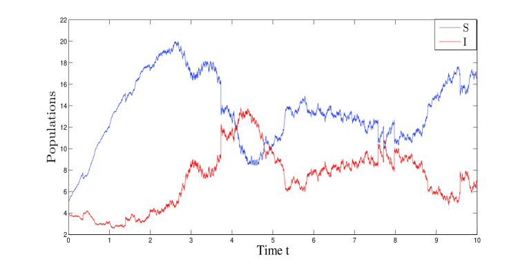
Figure 2: Susceptible and infected populations as functions of time in a situation of disease persistence.

The evolution of both susceptible and infected populations, as predicted by our Lévy jumps model (1), is illustrated in Fig. 2 in the case of disease persistence. We note that in this epidemic situation, all the four SICA compartments, i.e., the susceptible, the infected, the HIV-infected individuals under ART treatment (the so called chronic stage) with a viral load remaining low, and the HIV-infected individuals with AIDS clinical symptoms, persist. This is consistent with our theoretical findings of Section 4 concerning persistence.

6 Conclusion

In this work, we have considered and extended the epidemic SICA model of Silva and Torres [11] to a new stochastic model driven by both white noise and Lévy noise. This allows to better describe the sudden social fluctuations. The new SICA model was studied theoretically and some numerical simulations were also performed, which not only support the proved mathematical results but also illustrate the asymptotic behaviour of the solution. Firstly, with the help of Lyapunov’s analysis method, we have proved existence and uniqueness of a solution. Secondly, we have demonstrated that the model is well-posed, both mathematically and biologically, by establishing the boundedness of the solution, that is, $\limsup_{t\rightarrow\infty}N(t)\leq\dfrac{\Lambda}{\mu}$ a.s. and $\liminf_{t\rightarrow\infty}N(t)\geq\dfrac{\Lambda}{\mu+d}$ a.s., as well as the positivity of the solution. Thirdly, we have obtained an appropriate sufficient condition for extinction, showing that with an effective threshold of an eventual big magnitude of the volatility $\sigma$, $\frac{\beta^{2}}{2\sigma^{2}}<(\rho+\phi+\mu)+(\alpha+\omega)\frac{\Lambda}{\mu}$, the eradication of the disease occurs. Fourthly, a novel and significant sufficient condition

$$\liminf_{t\rightarrow\infty}<I(t)>\ \geq\frac{1}{(\rho+\phi+\mu)}\left(\frac{\beta\Lambda}{\mu+d}-(\rho+\phi+\mu)-\frac{\sigma^{2}\Lambda^{2}}{2\mu^{2}}\right)>0$$

and

$$\liminf_{t\rightarrow\infty}<S(t)>\frac{\Lambda\mu}{\Lambda\beta+\mu^{2}}>0$$

for persistence is obtained, which means that with an adopted small magnitude of volatility $\sigma$, the model is persistent in mean. Lastly, some numerical simulations were implemented that confirm and illustrate our mathematical results, give some supplementary insights and eventually helps a decision maker to select a good strategy to control the disease by means of the increasing or decreasing of the intensity of volatility or by taking into account and influencing the Lévy noise on the evolution of the variables of the system.

References

• [1] K. Akdim, A. Ez-Zetouni, J. Danane and K. Allali, Stochastic viral infection model with lytic and nonlytic immune responses driven by Lévy noise, Phys. A 549 (2020), Art. 124367, 11 pp.
• [2] K. Allali, J. Danane and Y. Kuang, Global analysis for an HIV infection model with CTL immune response and infected cells in eclipse phase, Appl. Sci. 7 (2017), no. 8, Art. 861, 18 pp.
• [3] W. Blanttner, R. C. Gallo and H. M. Temin, HIV causes AIDS, Science 241 (1988), 515–516.
• [4] P. De Leenheer and H. L. Smith, Virus dynamics: a global analysis, SIAM J. Appl. Math. 63 (2003), no. 4, 1313–1327.
• [5] A. Korobeinikov, Global properties of basic virus dynamics models, Bull. Math. Biol. 66 (2004), no. 4, 879–883.
• [6] M. Mahrouf, L. El Mehdi, M. Mehdi, K. Hattaf and N. Yousfi, A stochastic viral infection model with general functional response, Nonlinear Anal. Differ. Equ. 4 (2016), no. 9, 435–445.
• [7] M. A. Nowak and C. R. M. Bangham, Population dynamics of immune responses to persistent viruses, Science 272 (1996), no. 5258, 74–79.
• [8] M. Pitchaimani and M. Brasanna Devi, Effects of randomness on viral infection model with application, IFAC J. Syst. Control 6 (2018), 53–69.
• [9] R. Rajaji and M. Pitchaimani, Analysis of stochastic viral infection model with immune impairment, Int. J. Appl. Comput. Math. 3 (2017), no. 4, 3561–3574.
• [10] R. Sh. Liptser, A strong law of large numbers for local martingales, Stochastics 3 (1980), no. 3, 217–228.
• [11] C. J. Silva and D. F. M. Torres, A SICA compartmental model in epidemiology with application to HIV/AIDS in Cape Verde, Ecological Complexity 30 (2017), 70–75. arXiv:1612.00732
• [12] Q. Sun, L. Min and Y. Kuang, Global stability of infection-free state and endemic infection state of a modified human immunodeficiency virus infection model, IET Systems Biology 9 (2015), 95–103.
• [13] R. A. Weiss, How does HIV cause AIDS? Science 260 (1993), no. 5112, 1273–1279.
• [14] WHO, HIV/AIDS key facts, http://www.who.int/mediacentre/factsheets/fs360/en/index.html (accessed October 31, 2021)
• [15] Q. Zhang and K. Zhou, Stationary distribution and extinction of a stochastic SIQR model with saturated incidence rate, Math. Probl. Eng. 2019 (2019), Art. 3575410, 12 pp.
• [16] X. Zou and K. Wang, Numerical simulations and modeling for stochastic biological systems with jumps, Commun. Nonlinear Sci. Numer. Simul. 19 (2014), no. 5, 1557–1568.