Transport and Optimal Control of Vaccination Dynamics for COVID-19

Abstract

We develop a mathematical model for transferring the vaccine BNT162b2 based on the heat diffusion equation. Then, we apply optimal control theory to the proposed generalized SEIR model. We introduce vaccination for the susceptible population to control the spread of the COVID-19 epidemic. For this, we use the Pontryagin minimum principle to find the necessary optimality conditions for the optimal control. The optimal control problem and the heat diffusion equation are solved numerically. Finally, several simulations are done to study and predict the spread of the COVID-19 epidemic in Italy. In particular, we compare the model in the presence and absence of vaccination.

url]https://orcid.org/0000-0002-8956-2266

url]https://orcid.org/0000-0002-3531-0928

url]https://orcid.org/0000-0001-8641-2505

1 Introduction

BNT162b2 is an mRNA-based vaccine candidate against SARS-CoV-2, currently being developed by Pfizer and BioTech [9]. As announced on $9^{th}$ November 2020, BNT162b2 shows an efficacy against COVID-19 in patients without prior evidence of SARS-CoV-2 infection. A first interim efficacy analysis was conducted by an external, independent Data Monitoring Committee from the Phase 3 clinical study, and the case split, between vaccinated individuals and those who received the placebo, indicates a vaccine efficacy rate above $90\%$, at seven days after the second dose, of the 94 cases reviewed [20].

The major obstacle that must be overcome is related to the process of transporting the vaccine, which must be stored at $-70^{o}C$ [24]. Pfizer indicates that the vaccine will be distributed from its factories in the USA, Belgium and Germany. The American Wall Street Journal revealed that Pfizer has developed a special box packed with dry ice and a GPS tracker, which can hold 5000 doses of the vaccine under the right conditions for 10 days. Moreover, there is another obstacle related to the cost of the transportation boxes, where a similar box of 1200 doses in $-8^{o}C$ costs 6868 USD, which is very expensive.

The transport of the vaccine must comply with the general standards for drug storage and the recommended conditions. Although many transport vehicles are equipped with refrigeration devices, assuring recommended storage conditions, simple insulated transport boxes are often used. In this study, we use the heat diffusion equation and assume that the shape of the vaccine bottle is cylindrical [18]. We perform the calculations to find out an initial temperature that ensures the arrival of the vaccine while fulfilling the required condition of $-70^{o}C$, by using insulated transfer boxes with the internal temperature at $0^{o}C$ [22].

Optimal control is a mathematical theory that consists of finding a control that optimizes a functional on a domain described by a system of differential equations. This theory is applied in various fields of the engineering sciences: aeronautics, physics, biomedicine, etc. The Pontryagin minimum principle is used to find the necessary conditions for optimal controls [21].

Several models were presented to predict the spread of COVID-19 [14, 16, 17, 23, 26, 28]. These studies used the SIR and SEIR models [11] and the generalized SEIR model [19]. Most of them were implemented to evaluate the strategy of the preventive measures [2, 3, 4, 13, 15, 27].

In [1], the authors present a mathematical model to analyze the Ebola epidemic and two optimal control problems related to the transmission of Ebola disease with vaccination. In [19], the authors present a mathematical model to analyze the COVID-19 epidemic based on a dynamic mechanism that incorporates the intrinsic impact of hidden latent and infectious cases on the entire process of the virus transmission. The authors validate this model by analyzing data correlation and forecasting available general data. Their model reveals the key parameters of the COVID-19 epidemic. Here, we modify the model analyzed in [19] and consider an optimal control problem. More precisely, we introduce an extra variable for the number of vaccines used. Secondly, we study the associated optimal control problem, solving it numerically. Moreover, in order to find out the main parameters, we have performed a numerical simulation of the spread of COVID-19 in Italy from $01^{st}$ November 2020 to $31^{th}$ January 2021. Finally, we have presented another simulation to find the optimal control, and we have compared the models with and without vaccination.

The paper is organized as follows. We begin by formulating the vaccination transport model in Section 2. In Section 3, we recall the generalized SEIR model. Then, in Section 4, we formulate the generalized SEIR model with vaccination as an optimal control problem. The obtained optimal control problem is solved numerically in Section 5. In Section 6, we present a discussion concerning the spread of COVID-19 in Italy during three months, starting from $1^{st}$ November 2020. We end with Section 7 of conclusion, including some future research directions.

2 Vaccine transport model

In this section, we present a model to maintain the effectiveness of the vaccine while transporting it from the factory storage area to the desired destination. The aim is to know the initial temperature that maintains the effectiveness of the vaccine, less than $-70^{o}$, and this by using the available mobile boxes at $0^{o}C$. Thus, we propose the following mathematical model:

$$\left\{\begin{array}[]{l l}\displaystyle\frac{\partial T(t,x,y,z)}{\partial t}-\alpha\nabla^{2}T(t,x,y,z)=0,&\text{on }\ [0,t_{*}]\times\Omega,\\ T(t_{*},x,y,z)=-70^{o}C,&\forall(x,y,z)\in\Omega,\\ T(t,x,y,z)=0^{o}C,&\forall(t,x,y,z)\in[0,t_{*}]\times\partial\Omega,\\ \Omega=\left\{(x,y,z)\in\mathbb{R}^{3}:\ x^{2}+y^{2}<r^{2},\ 0<z<h\right\},\\ \partial\Omega=\left\{(x,y,z)\in\mathbb{R}^{3}:\ x^{2}+y^{2}=r^{2},\ 0\leq z\leq h\right\},\\ \end{array}\right.$$ (1)

where $T(t,x,y,z)$ represents the temperature of the vaccine at the point $(x,y,z)$ and the time $t$; $t_{*}$ is the arrival time of the vaccine; and $0^{o}C$ is the temperature inside the box. The sets $\Omega$ and $\partial\Omega$ represent the interior and the border of the bottle containing the vaccine, respectively, $r$ and $h$ are the radius and height of the bottle, respectively, and $\alpha$ is the thermal diffusivity defined by

$$\alpha=\frac{k}{\rho c_{\rho}},$$ (2)

where $k$ is the thermal conductivity, $c_{\rho}$ is the specific heat capacity, and $\rho$ is the density.

3 Initial mathematical model for COVID-19

The generalized SEIR model proposed by Peng et al. [19] is expressed by a seven-dimensional dynamical system defined by

$$\left\{\begin{array}[]{l l}\dot{S}(t)=-\dfrac{\beta S(t)I(t)}{N}-\omega S(t),\\ \dot{E}(t)=\dfrac{\beta S(t)I(t)}{N}-\gamma E(t),\\ \dot{I}(t)=\gamma E(t)-\delta I(t),\\ \dot{Q}(t)=\delta I(t)-\lambda(t)Q(t)-\kappa(t)Q(t),\\ \dot{R}(t)=\lambda(t)Q(t),\\ \dot{D}(t)=\kappa(t)Q(t),\\ \dot{P}(t)=\omega S(t),\\ \end{array}\right.$$ (3)

where the state variables are subjected to the following initial conditions:

$$S(0)=S_{0},\ E(0)=E_{0},\ I(0)=I_{0},\ Q(0)=Q_{0},\ R(0)=R_{0},\ D(0)=D_{0},\ P(0)=P_{0}.$$

In this model, the population is divided into the following compartments: susceptible individuals $S(t)$, exposed individuals $E(t)$, infected individuals $I(t)$, quarantined individuals $Q(t)$, recovered individuals $R(t)$, death individuals $D(t)$, and insusceptible/protected individuals $P(t)$. These variables, in total, constitute the whole population, denoted by $N$:

$$N=S(t)+E(t)+I(t)+Q(t)+R(t)+D(t)+P(t).$$

The parameters $\omega$, $\beta$, $\gamma$, $\delta$, $\lambda(t)$, and $\kappa(t)$ represent the protection rate, infection rate, inverse of the average latent time, rate at which infectious people enter in quarantine, time-dependent recovery rate, and the time-dependent mortality rate, respectively. The recovery $\lambda(t)$ and mortality $\kappa(t)$ rates are analytical functions of time, defined by

$$\lambda(t)=\frac{\lambda_{1}}{1+\exp(-\lambda_{2}(t-\lambda_{3}))},$$ (4)

$$\kappa(t)=\frac{\kappa_{1}}{\exp(\kappa_{2}(t-\kappa_{3}))+\exp(-\kappa_{2}(t-\kappa_{3}))},$$ (5)

where the parameters $\lambda_{1}$, $\lambda_{2}$, $\lambda_{3}$, $\kappa_{1}$, $\kappa_{2}$ and $\kappa_{3}$ are empirically determined in Section 6.

4 Mathematical model for COVID-19 with vaccination

We now introduce the vaccine for the susceptible population in order to control the spread of COVID-19. Let us introduce in model (3) a control function $u(t)$ and an extra variable $W(t)$, $t\in[0,t_{f}]$, representing the percentage of susceptible individuals being vaccinated and the number of vaccines used, respectively, with

$$\frac{dW}{dt}(t)=u(t)S(t),\ \ \text{subject to the initial condition}\ W(0)=0,\\$$ (6)

where $t_{f}$ represents the final time of the vaccination program. Hence, our model with vaccination is given by the following system of eight nonlinear ordinary differential equations:

$$\left\{\begin{array}[]{l l}\dot{S}(t)=-\dfrac{\beta S(t)I(t)}{N}-\omega S(t)-u(t)S(t),\\ \dot{E}(t)=\dfrac{\beta S(t)I(t)}{N}-\gamma E(t),\\ \dot{I}(t)=\gamma E(t)-\delta I(t),\\ \dot{Q}(t)=\delta I(t)-\lambda(t)Q(t)-\kappa(t)Q(t),\\ \dot{R}(t)=\lambda(t)Q(t),\\ \dot{D}(t)=\kappa(t)Q(t),\\ \dot{P}(t)=\omega S(t),\\ \dot{W}(t)=u(t)S(t),\end{array}\right.$$ (7)

where the state variables are subject to the initial conditions:

$$\begin{split}S(0)&=S_{0},\ E(0)=E_{0},\ I(0)=I_{0},\ Q(0)=Q_{0},\\ R(0)&=R_{0},\ D(0)=D_{0},\ P(0)=P_{0},\ W(0)=W_{0}=0.\end{split}$$

A schematic diagram of model (7) is given in Figure 1.

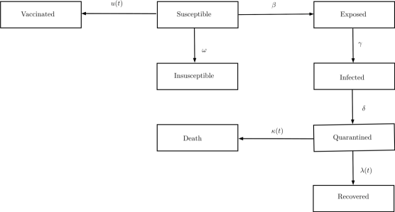
Figure 1: Schematic diagram of the generalized SEIR model with vaccination.

5 Optimal Control

We consider the model with vaccination (7) and formulate an optimal control problem to determine the vaccination strategy $u$ that minimizes the cost of treatment and vaccination:

$$\min_{u}J(u)=\int\limits_{0}^{t_{f}}\left(w_{1}I^{2}(t)+w_{2}u^{2}(t)\right)dt,$$ (8)

where $w_{1}$ and $w_{2}$ represent the weights associated with the cost of treatment and vaccination, respectively. We assume that the control function $u$ takes values between $0$ and $1$. When $u(t)=0$, no susceptible individual is vaccinated at time $t$ and if $u(t)=1$, then all susceptible individuals are vaccinated at time $t$.

Let $x(t)=(x_{1}(t),\ldots,x_{8}(t))=(S(t),E(t),I(t),Q(t),R(t),D(t),P(t),W(t))\in\mathbb{R}^{8}$. The optimal control problem consists in finding the control $\tilde{u}$ and the associated optimal trajectory $\tilde{x}$, satisfying the control system (7) with the given initial conditions

$$x(0)=(S_{0},E_{0},I_{0},Q_{0},R_{0},D_{0},P_{0},W_{0}),$$ (9)

where the control $\tilde{u}\in\Gamma$,

$$\Gamma=\{u(\cdot)\in L^{\infty}([0,t_{f}],\mathbb{R})\ :\ 0\leq u(t)\leq 1,\ t\in[0,t_{f}]\},$$ (10)

minimizes the objective functional (8). With the new variables, problem (7)–(10) becomes

$$\begin{gathered}\min\limits_{u\in\Gamma}J(u)=\int\limits_{0}^{t_{f}}\left(w_{1}x_{3}^{2}(t)+w_{2}u^{2}(t)\right)dt,\\ \dot{x}(t)=A(t)x(t)+B(x(t))u(t)+f(x(t)),\quad x(0)=(S_{0},E_{0},I_{0},Q_{0},R_{0},D_{0},P_{0},W_{0}),\end{gathered}$$ (11)

where

$$A(t)=\left(\begin{array}[]{cccccccc}-\omega&0&0&0&0&0&0&0\\ 0&-\gamma&0&0&0&0&0&0\\ 0&\gamma&-\delta&0&0&0&0&0\\ 0&0&\delta&-\lambda(t)-\kappa(t)&0&0&0&0\\ 0&0&0&\lambda(t)&0&0&0&0\\ 0&0&0&\kappa(t)&0&0&0&0\\ \omega&0&0&0&0&0&0&0\\ 0&0&0&0&0&0&0&0\\ \end{array}\right),$$

$$B(x)=(-x_{1},\ 0,\ 0,\ 0,\ 0,\ 0,\ 0,\ x_{1})^{T},$$

$$f(x)=\left(-\frac{\beta x_{1}x_{3}}{N},\ \frac{\beta x_{1}x_{3}}{N},\ 0,\ 0,\ 0,\ 0,\ 0,\ 0\right)^{T}.$$

The existence of the optimal control $\tilde{u}$ and the associated optimal trajectory $\tilde{x}$ comes from the convexity of the integrand of the cost functional (8) with respect to the control $u$ and the Lipschitz property of the state system with respect to the state vector $x(t)$ (see [7] for existence results of optimal solutions). According to the Pontryagin Minimum Principle [21], if $\tilde{u}\in\Gamma$ is optimal for the problem (11) with fixed final time $t_{f}$, then there exists $\psi\in AC([0,t_{f}],\mathbb{R}^{8})$, $\psi(t)=(\psi_{1}(t),\ldots,\psi_{8}(t))$, called the adjoint vector, such that

$$\dot{x}=\frac{\partial H}{\partial\psi}\ \text{ and }\ \dot{\psi}=-\frac{\partial H}{\partial x},$$

where the Hamiltonian $H$ is defined by

$$H(t,x,\psi,u)=w_{1}x_{3}^{2}+w_{2}u^{2}+\psi^{T}\left(A(t)x+B(x)u+f(x)\right).$$ (12)

The adjoint functions satisfy

$$\dot{\psi}=-\frac{\partial H}{\partial x}=\bar{A}(t,x,u)\psi+\bar{B}(x),$$ (13)

where

$$\bar{A}(t,x,u)=\left(\begin{array}[]{cccccccc}\frac{\beta x_{3}}{N}+\omega+u&-\frac{\beta x_{3}}{N}&0&0&0&0&-\omega&-u\\ 0&\gamma&-\gamma&0&0&0&0&0\\ \frac{\beta x_{1}}{N}&-\frac{\beta x_{1}}{N}&\delta&-\delta&0&0&0&0\\ 0&0&0&\lambda(t)+\kappa(t)&-\lambda(t)&-\kappa(t)&0&0\\ 0&0&0&0&0&0&0&0\\ 0&0&0&0&0&0&0&0\\ 0&0&0&0&0&0&0&0\\ 0&0&0&0&0&0&0&0\end{array}\right),$$

$$\bar{B}(x)=\left(0,\ 0,\ -2w_{1}x_{3},\ 0,\ 0,\ 0,\ 0,\ 0\right)^{T}.$$

The minimality condition

$$H(t,\tilde{x}(t),\tilde{\psi}(t),\tilde{u}(t))=\min\limits_{u\in[0,1]}H(t,\tilde{x}(t),\tilde{\psi}(t),u)$$ (14)

holds almost everywhere on $[0,t_{f}]$. Moreover, the transversality conditions assert that $\tilde{\psi}_{i}(t_{f})=0$, $i=1,\ldots,8$. It follows from the the Pontryagin minimum principle that the extremal control $\tilde{u}^{p}$ is given by

$$\tilde{u}^{p}(t)=\left\{\begin{array}[]{ll}\tilde{u}(t)&\text{if}\ \ 0<\tilde{u}(t)<1,\\ 0&\text{if}\ \ \tilde{u}(t)\leq 0,\\ 1&\text{if}\ \ \tilde{u}(t)\geq 1,\\ \end{array}\right.$$ (15)

where

$$\tilde{u}(t)=\frac{\tilde{x}_{1}(t)\left(\tilde{\psi}_{1}(t)-\tilde{\psi}_{8}(t)\right)}{2w_{2}}.$$ (16)

6 Numerical Results

The current study aims to find the initial temperature to maintain the effectiveness of the vaccine during the transportation process, as well as determining an optimal vaccination strategy to limit the spread of COVID-19 in Italy. For that we reduce the costs of treatment and vaccination, during the three months starting from $1^{st}$ November 2020. We use the MATLAB R2020b program to perform all numerical computations. The initial conditions and real data are taken from the public database Dati COVID-19 Italia, available from https://github.com/pcm-dpc/COVID-19.

We assume $r=3\ cm$, $h=4\ cm$, $\alpha=0.0137\ W/(m\cdot C)$, $\rho=2600\ kg/m^{3}$, $c_{\rho}=750\ W\cdot s/(kg\cdot C)$ and $t_{*}=7200\ s$, with the heat transfer coefficient equal to $1$. In Fig. 2 we present the numerical solution of the heat diffusion equation (1), which gives the initial temperature equal to $-94.5^{o}C$.

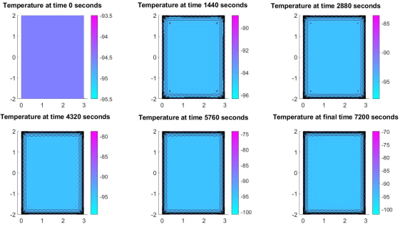
Figure 2: Numerical solution of the heat diffusion equation (1).

We consider the following initial guesses: $\omega=0.06$, $\beta=1$, $\gamma=5$, $\delta=0.5$, $(\lambda_{1},\lambda_{2},\lambda_{3})=(0.01,\ 0.1,\ 10)$ and $(\kappa_{1},\kappa_{2},\kappa_{3})=(0.001,\ 0.001,\ 10)$.

The parameters of the generalized SEIR model are computed simultaneously by a nonlinear least-squares solver [8]. These parameters over the period starting from $1^{st}$ November 2020 till $31^{th}$ January 2021 are: $\omega=0.0547$, $\beta=0.5425$, $\gamma=0.0873$, $\delta=0.3425$, $(\lambda_{1},\lambda_{2},\lambda_{3})=(0.0999,\ 0.0501,\ 38.8542)$ and $(\kappa_{1},\kappa_{2},\kappa_{3})=(0.0021,\ 0.0125,\ 66.6652)$.

In Fig. 3 we show the recovery rate $\lambda(t)$ and the mortality rate $\kappa(t)$.

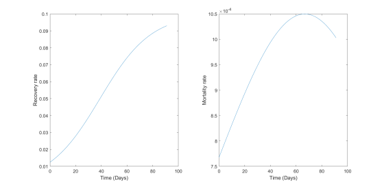
Figure 3: The recovery and mortality rates.

We fixed $w_{1}=w_{2}=1$. The numerical solutions to the non-linear differential equations that represent the generalized SEIR model (3), the generalized SEIR model with vaccination (7), and the real data of the quarantined, recovered and death cases, from $1^{st}$ November till $6^{th}$ December 2021, are shown in Fig. 4.

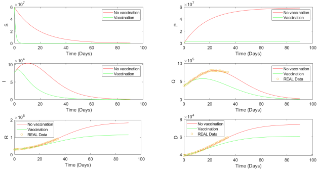
Figure 4: The solutions of the generalized SEIR models (3) and (7), respectively without and with vaccination, and real data of Italy from $1^{st}$ November till $6^{th}$ December 2021 with total population of $N=60.480.000$.

In Fig. 5 we present the optimal control (15)–(16) and the number of vaccines used starting from $1^{st}$ November 2020 till $31^{th}$ January 2021.

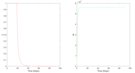
Figure 5: The optimal control $\tilde{u}$ (left) and the number of vaccines $W(t)$ (right).

The orange curves in Fig. 4 represent the real data for the number of the quarantine, recovery and death cases in Italy starting from $1^{st}$ November till $6^{th}$ December $2020$. The red curves in Fig. 4 represent the solutions of the generalized SEIR model (3) without vaccination, and they simulate what happen from the beginning of November to the end of January. There is an increase in the number of the recovered, death and insusceptible cases that reach, respectively, $1.830.000$, $74.050$ and $58.130.000$ cases. The red curves for both the number of infected and quarantined individuals have their higher limit values of $103500$ cases on $11^{th}$ November and $798.500$ on $25^{th}$ November, respectively, reaching the values $614$ and $22.640$ cases on $31^{th}$ January $2021$, respectively. We note that the number of susceptible individuals gradually decrease, reaching $416.600$ cases at the end of January $2021$.

The green curves in Fig. 4 represent the solutions of the generalized SEIR model (7) with vaccination, and they simulate what happened from the beginning of November to the end of January. There is an increase in the number of recovered, death and insusceptible cases that reach, respectively, $1.135.000$, $60.560$ and $3.076.000$ cases. The green curves for both the number of infected and quarantined individuals have their higher limit values of $84.800$ cases on $4^{th}$ November and $577.600$ cases on $15^{th}$ November, respectively, reaching $55$ and $7.237$ cases on $31^{th}$ January $2021$, respectively. We note that the number of susceptible individuals decrease rapidly reaching $0$ cases on $19^{th}$ November $2020$.

The red curve in Fig. 5 shows that the optimal vaccination of 100 percent of the susceptible individuals takes 19 days, followed by a rapid decrease in the number of susceptible individuals, which means they move to the class of vaccinated. The green curve in Fig. 5 shows the necessary number of vaccines to eliminate COVID-19, which is estimated at 56.200.100 doses. The total number of vaccinated and insusceptible individuals equal to 59.276.100 of the total Italian population of 60.480.000.

7 Conclusion

Our results show the importance of the vaccine for COVID-19 control and also the best result that could be obtained if the number of available vaccines satisfies the needs of the population and are distributed according with the theory of optimal control.

Here our optimal control problem has only one control: the vaccine. In reality, there are several other factors to take into account and other variables to control. In a future work, we would like to use the support maximum principle [5, 6, 10], as well as the hybrid direction method [25], to elaborate a primal-dual method for solving a more realistic optimal control problem, in presence of multiple inputs [12].

References

- [1] I. Area, F. Ndaïrou, J. J. Nieto, C. J. Silva and D. F. M. Torres, Ebola model and optimal control with vaccination constraints, J. Ind. Manag. Optim. 14 (2018), no. 2, 427–446. arXiv:1703.01368
- [2] D. K. Bagal, A. Rath, A. Barua and D. Patnaik, Estimating the parameters of susceptible-infected-recovered model of COVID-19 cases in India during lockdown periods, Chaos Solitons Fractals 140 (2020), Art. 110154, 12 pp.
- [3] A. Ballesteros et al., Hamiltonian Structure of Compartmental Epidemiological models, Physica D: Nonlinear Phenomena 413 (2020), Art. 132656, 18 pp.
- [4] H. W. Berhe and O. D. Makinde, Optimal Control and Cost-Effectiveness Analysis for Dysentery Epidemic Model, Applied Mathematics and Information Sciences 12 (2018), no. 6, 1183–1195.
- [5] M. O. Bibi, Methods for solving linear-quadratic problems of optimal control, PhD thesis in Applied Mathematics, University of Minsk, 1985.
- [6] M. O. Bibi, Optimization of a linear dynamic system with double terminal constraint on the trajectories, Optimization 30 (1994), no. 4, 359–366.
- [7] L. Cesari, Optimization—theory and applications, Applications of Mathematics (New York), 17, Springer-Verlag, New York, 1983.
- [8] E. Cheynet, Generalized SEIR Epidemic Model (fitting and computation), 28 Sept 2020. https://github.com/ECheynet/SEIR/tree/v4.8.7
- [9] E. Edward et al., Safety and Immunogenicity of Two RNA-Based Covid-19 Vaccine Candidates, N. Engl. J. Med. 383 (2020), 2439–2450.
- [10] F. Ghellab and M. O. Bibi, Optimality and suboptimality criteria in a quadratic problem of optimal control with a piecewise linear entry, International Journal of Mathematics in Operational Research 19 (2021), no. 1, 1–18.
- [11] W. O. Kermack and A. G. McKendrick, A contribution to the mathematical theory of epidemics, Proc. R. Soc. Lond., Ser. A 115 (1927), 700–721.
- [12] N. Khimoum and M. O. Bibi, Primal-dual method for solving a linear-quadratic multi-input optimal control problem, Optimization Letters 14 (2020), 653–669.
- [13] S. A. Lauer, K. H. Grantz, Q. Bi, F. K. Jones and Q. Zheng, H. R. Meredith, A. S. Azman, N. G. Reich and J. Lessler, The incubation period of coronavirus disease 2019 (COVID-19) from publicly reported confirmed cases: Estimation and application, Annals of Internal Medicine 172 (2020), no. 9, 577–583.
- [14] A. P. Lemos-Paião, C. J. Silva and D. F. M. Torres, A new compartmental epidemiological model for COVID-19 with a case study of Portugal, Ecological Complexity 44 (2020) Art. 100885, 8 pp. arXiv:2011.08741
- [15] Q. Lin, S. Zhao, D. Gao, Y. Lou, S. Yang and S. S. Musa, M. H. Wang, Y. Cai, W. Wang, L. Yang and D. He, A conceptual model for the coronavirus disease 2019 (COVID-19) outbreak in Wuhan, China with individual reaction and governmental action, International Journal of Infectious Diseases 93 (2020), 211–216.
- [16] R. Lu et al., Genomic characterisation and epidemiology of 2019 novel coronavirus: Implications for virus origins and receptor binding, The Lancet 395 (2020), no. 10224, 565–574.
- [17] F. Ndaïrou, I. Area, J. J. Nieto, C. J. Silva and D. F. M. Torres, Fractional model of COVID-19 applied to Galicia, Spain and Portugal, Chaos Solitons Fractals 144 (2021), Art. 110652, 7 pp. arXiv:2101.01287
- [18] M. O. Necati, Heat Conduction, Interscience Publishers John Wiley & Sons, Inc. New York, 1993.
- [19] L. Peng, W. Yang, D. Zhang, C. Zhuge and L. Hong, Epidemic analysis of COVID-19 in China by dynamical modeling, preprint, arXiv:2002.06563v2, 25 June 2020. https://doi.org/10.1101/2020.02.16.20023465
- [20] F. P. Polack et al., Safety and efficacy of the BNT162b2 mRNA Covid-19 vaccine, N. Engl. J. Med. 383 (2020), 2603–2615.
- [21] L. S. Pontryagin, V. G. Boltyanskii, R. V. Gamkrelidze and E. F. Mishchenko, The mathematical theory of optimal processes, Translated from the Russian by K. N. Trirogoff; edited by L. W. Neustadt, Interscience Publishers John Wiley & Sons, Inc. New York, 1962.
- [22] M. Shashkov and S. Steinberg, Solving Diffusion Equations with Rough Coefficients in Rough Grids, Journal of Computational Physics 129 (1996), 383–405.
- [23] C. J. Silva et al., Optimal control of the COVID-19 pandemic: controlled sanitary deconfinement in Portugal, Scientific Reports 11 (2021), Art. 3451, 15 pp. arXiv:2009.00660
- [24] A. B. Vogel et al., A prefusion SARS-CoV-2 spike RNA vaccine is highly immunogenic and prevents lung infection in non-human primates, bioRxiv (2020), DOI: https://doi.org/10.1101/2020.09.08.280818.
- [25] M. A. Zaitri, M. O. Bibi and M. Bentobache, A hybrid direction algorithm for solving optimal control problems, Cogent Math. Stat. 6 (2019), no. 1, Art. ID 1612614, 12 pp.
- [26] M. Zamir, T. Abdeljawad, F. Nadeem, A. Wahid and A. Yousef, An optimal control analysis of a COVID-19 model, Alexandria Engineering Journal 60 (2021), no. 3, 2875–2884.
- [27] Z. Zhao, X. Li, F. Liu, G. Zhu, C. Ma and L. Wang, Prediction of the COVID-19 spread in African countries and implications for prevention and control: A case study in South Africa, Egypt, Algeria, Nigeria, Senegal and Kenya, Science of the Total Environment 729 (2020), Art. 138959, 10 pp.
- [28] H. Zine, A. Boukhouima, E. M. Lotfi, M. Mahrouf, D. F. M. Torres and N. Yousfi, A stochastic time-delayed model for the effectiveness of Moroccan COVID-19 deconfinement strategy, Math. Model. Nat. Phenom. 15 (2020), Art. 50, 14 pp. arXiv:2010.16265