Multi-cell Non-coherent Over-the-Air Computation for Federated Edge Learning

Abstract

In this paper, we propose a framework where over-the-air computation (OAC) occurs in both uplink (UL) and downlink (DL), sequentially, in a multi-cell environment to address the latency and the scalability issues of federated edge learning (FEEL). To eliminate the channel state information (CSI) at the edge devices and edge servers and relax the time-synchronization requirement for the OAC, we use a non-coherent computation scheme, i.e., -based (FSK-MV). With the proposed framework, multiple ESs function as the aggregation nodes in the UL and each ES determines the MVs independently. After the ESs broadcast the detected MVs, the EDs determine the sign of the gradient through another OAC in the DL. Hence, inter-cell interference is exploited for the OAC. In this study, we prove the convergence of the non-convex optimization problem for the FEEL with the proposed OAC framework. We also numerically evaluate the efficacy of the proposed method by comparing the test accuracy in both multi-cell and single-cell scenarios for both homogeneous and heterogeneous data distributions.

I Introduction

OAC refers to the computation of mathematical functions by exploiting the superposition property of wireless multiple-access channel [1]. It has been initially considered in wireless sensor networks to reduce the latency due to a large number of nodes [2, 3, 4]. Recently, it has been shown that OAC is also a prominent solution to address the latency issue of FEEL [5] or distributed training problems in a wireless network [6]. Nevertheless, apart from a few work, e.g., [7], FEEL with OAC is primarily investigated in a single cell in the UL although the practical wireless networks often consist of multiple cells. In this study, we address this issue and propose a framework for FEEL based on a non-coherent OAC scheme in both UL and DL in a multi-cell environment.

One of the major challenges in the OAC is the detrimental impact of wireless channels on the coherent symbol superposition. To address this issue, a majority of the state-of-the-art solutions rely on pre-equalization techniques. For instance, in [8] and [9], broadband analog aggregation (BAA) over orthogonal frequency division multiplexing (OFDM) with truncated-channel inversion (TCI) is investigated to obtain unbiased estimates of the weights or gradients. In [10], one-bit broadband digital aggregation (OBDA), inspired by distributed training by MV with the sign stochastic gradient descend (signSGD) [11], is proposed to facilitate the implementation of FEEL for a practical wireless system, which also uses TCI. In [12], instead of TCI, the conjugate of the channel is utilized. In [13] and [14], it is assumed that the CSI for each ED is available at the ES. The impact of the channel on OAC is mitigated through beamforming techniques. In this paper, to overcome this challenge and requiring CSI access at the EDs and the ESs, a non-coherent computation scheme is deployed.

The state-of-the-art OAC techniques are often suitable for a single cell where the OAC occurs in the UL due to the pre-equalization. In addition, pre-equalization techniques require sample-level precise time synchronization, which causes another shortcoming when multiple aggregation nodes exist in a wireless network. In [15] and [16], non-coherent computation through FSK-MV and -based (PPM-MV) are investigated for FEEL in a single cell scenario. The main strategy in these studies is to dedicate two resources where either of the two resources are activated based on the sign of the gradient. The MV at the ES is detected through an energy detector. Since the information is not encoded in the amplitude or the phase in this strategy, the need for CSI at the EDs and the ES are eliminated and the precise time-synchronization requirement is relaxed. Because of these unique features, we consider non-coherent OAC in a multi-cell environment.

In this study, we propose an OAC framework where OAC occurs in both UL and DL in a multi-cell environment with FSK-based MV. As opposed to a single-cell solution, multiple ESs first detect the MVs through the UL OAC. Afterward, each ED determines the sign of the gradient by aggregating the ESs’ signals in the DL with another OAC. We show the convergence of the non-convex loss function problem for FEEL with the proposed scheme and evaluate the proposed framework numerically. We show that the efficacy of the proposed framework by comparing it with a single-cell scenario for both homogeneous and heterogeneous data distributions.

Notation: ${\mathbb{E}}\left[\cdot\right]$ is the expectation operation. $\mathbb{I}\left[{\cdot}\right]$ is the indicator function. The function $\operatorname{sign}(\cdot)$ results in $1$, $-1$, or $\pm 1$ at random for a positive, a negative, or a zero-valued argument.

II System Model

Consider a multi-cell wireless network with $K$ EDs and $S$ ESs. We assume that the frequency synchronization in the network is handled through a control mechanism. We consider time synchronization errors among the EDs (and the ESs) and the maximum difference between the time of arrivals of the signals at the desired receiver’s location is $T_{\rm sync}$ seconds, where $T_{\rm sync}$ is equal to the reciprocal to the signal bandwidth. We assume that the UL signal-to-noise ratio (SNR) at an ES is $1/\sigma_{\rm ES}^{2}$ when an ED is located at the reference distance $r_{\rm UL}$. We then set the received signal power of the $k$th ED at the $s$th ES as $P^{k,s}_{\rm ED}={r_{k,s}}^{-\alpha}/{r_{\rm UL}^{-\alpha}}$, where $r_{k,s}$ is the link distance between the $k$th ED and the $s$th ES, and $\alpha$ is the path loss exponent. Similarly, we define the DL SNR at an ED is $1/\sigma_{\rm ED}^{2}$ when the distance between an ED and an ES is equal to the reference distance $r_{\rm DL}$. We then set the received signal power of the $s$th ES at the $k$th ED as $P^{s,k}_{\rm ES}={{r_{s,k}}^{-\alpha}}/{r_{\rm DL}^{-\alpha}}$.

II-A Signal Model in Uplink and Downlink

In this study, the EDs in the UL and the ESs in the DL access the wireless channel on the same time-frequency resources simultaneously with $N$ OFDM symbols consisting of $M$ active subcarriers. We assume that the cyclic prefix (CP) duration is larger than $T_{\rm sync}$ and the maximum-excess delay of the channel. Considering independent frequency-selective channels between the EDs and the ESs, the superposed symbol on the $m$th subcarrier of the $n$th OFDM symbol at the $s$th ES for the $t$th communication round of FEEL can be written as

$$r^{t,{s,m,n}}_{\rm ES}=\sum_{k=1}^{K}\sqrt{P^{s,k}_{\rm ED}}h^{t,{s,k,m,n}}_{\rm UL}t_{\rm ED}^{t,{k,m,n}}+\omega^{t,{s,m,n}}_{\rm ES}~{},$$ (1)

where $h^{t,{s,k,m,n}}_{\rm UL}\in\mathbb{C}$ is the channel coefficient between the $s$th ES and the $k$th ED, $t_{\rm ED}^{t,{k,m,n}}\in\mathbb{C}$ is the transmitted symbol from the $k$th ED, and $\omega^{t,{k,m,n}}_{\rm ES}$ is the symmetric additive white Gaussian noise (AWGN) with zero mean and the variance $\sigma_{\rm ES}^{2}$ on the $m$th subcarrier for $m\in\{0,1,\hbox to10.00002pt{.\hss.\hss.},M-1\}$ and $n\in\{0,1,\hbox to10.00002pt{.\hss.\hss.},N-1\}$. Similarly, the received symbol on the $m$th subcarrier of the $n$th OFDM symbol at the $k$th ED for the $t$th communication round in the DL can be shown as

$$r^{t,{k,m,n}}_{\rm ED}=\sum_{s=1}^{S}\sqrt{P^{s,k}_{\rm ES}}h^{t,{s,k,m,n}}_{\rm DL}t_{\rm ES}^{t,{s,m,n}}+\omega^{t,{k,m,n}}_{\rm ED}~{},$$ (2)

where $h^{t,{s,k,m,n}}_{\rm DL}\in\mathbb{C}$ is the channel coefficient between the $s$th ES and the $k$th ED, $t_{\rm ES}^{t,{s,m,n}}\in\mathbb{C}$ is the transmitted symbol from the $s$th ES, and $\omega^{t,{k,m,n}}_{\rm ED}$ is the symmetric AWGN with zero mean and the variance $\sigma_{\rm ED}^{2}$ on the $m$th subcarrier.

II-B Problem Statement and Learning Model

Let $\textbf{w}^{(t)}_{k}\in\mathbb{R}^{Q}$ denote the model parameters at the $k$th ED for the $t$th communication round, and $Q$ is the number of parameters. The local data set containing labeled data samples at the $k$th ED as $\{({\textrm{{x}}}_{{\ell}},{y}_{{\ell}})\}\in\mathcal{D}_{k}$, where ${\textrm{{x}}}_{{\ell}}$ and ${y}_{{\ell}}$ are the ${\ell}$th data sample and its associated label respectively. In this study, unlike to a classical FEEL problem, to capture the model test accuracy for each ED under heterogeneous data distribution, we define a personalized global loss function at the $k$th ED for a given $\textbf{w}^{(t)}_{k}$ as

$$F_{k}(\textbf{w}^{(t)}_{k})=\frac{1}{|\mathcal{G}_{k}|}\sum_{\forall({\textrm{{x}}}_{{\ell}},{y}_{{\ell}})\in\mathcal{G}_{k}}f({\textbf{w}^{(t)}_{k}},{\textrm{{x}}}_{{\ell}},{y}_{{\ell}})~{},$$ (3)

where $\mathcal{G}_{k}=\{({\textrm{{x}}}_{{\ell}},{y}_{{\ell}})\in\mathcal{G}|{y}_{{\ell}}\in\mathcal{C}_{k}\}$ for $\mathcal{G}=\mathcal{D}_{1}\cup\mathcal{D}_{2}\cup\hbox to10.00002pt{.\hss.\hss.}\cup\mathcal{D}_{K}$, and $\mathcal{C}_{k}$ is the set of distinct labels in the dataset of the $k$th ED. $f({\textbf{w}^{(t)}_{k}},{\textrm{{x}}}_{{\ell}},{y}_{{\ell}})$ is the sample loss function that measures the labelling error for $({\textrm{{x}}}_{{\ell}},{y}_{{\ell}})$ for the parameters ${\textbf{w}^{(t)}_{k}}$ at the $k$th ED. The personalized federated learning (FL) problem can then be defined as

$${\textbf{w}_{k}^{*}}=\arg\min_{\textbf{w}_{k}}F_{k}(\textbf{w}^{(t)}_{k})~{}.$$ (4)

To solve (4), a full-batch gradient descent with the learning rate $\eta$ is given by $\textbf{w}^{(t+1)}_{k}=\textbf{w}^{(t)}_{k}-\eta\textbf{g}_{k}^{(t)}$, and

$$\textbf{g}_{k}^{(t)}=\nabla F_{k}(\textbf{w}^{(t)}_{k})=\frac{1}{|\mathcal{G}_{k}|}\sum_{\forall({\textrm{{x}}}_{{\ell}},{y}_{{\ell}})\in\mathcal{G}_{k}}\nabla f(\textbf{w}^{(t)}_{k},{\textrm{{x}}}_{{\ell}},{y}_{{\ell}})~{},$$ (5)

where the $i$th element of $\textbf{g}_{k}^{(t)}$ is ${g}_{k,i}^{(t)}$, which is the gradient of $F_{k}(\textbf{w}^{(t)}_{k})$ with respect to $w^{(t)}_{k,i}$.

In this study, our main goal is to solve (4) in a wireless network consisting of multiple cells, where the data sharing among EDs is not allowed to promote data privacy. To this end, we consider FEEL and reduce the communication latency by adopting an OAC scheme, i.e., FSK-MV [15], which is originally proposed in the UL for a single cell (i.e., $S=1$). With this scheme, the $k$th ED first calculates the local stochastic gradient as

$${\tilde{\textbf{g}}}_{k}^{(t)}=\frac{1}{n_{\rm b}}\sum_{\forall({\textrm{{x}}}_{{\ell}},{y}_{{\ell}})\in\mathcal{\tilde{D}}_{k}}\nabla f(\textbf{w}^{(t)}_{k},{\textrm{{x}}}_{{\ell}},{y}_{{\ell}})~{},$$ (6)

where ${\tilde{\textbf{g}}}_{k}^{(t)}$ is the local gradient where its $i$th element is ${\tilde{g}^{(t)}}_{k,i}$ and $\mathcal{\tilde{D}}_{k}\subset\mathcal{D}_{k}$ is the selected data batch from the local data set with the batch size, $n_{\rm b}=|\mathcal{\tilde{D}}_{k}|$. Each ED then obtains the transmit symbols in the UL as follows: Consider a mapping from $i\in\{1,...,Q\}$ to the distinct pairs $(m^{+},n^{+})$ and $(m^{-},n^{-})$ for $m^{+},m^{-}\in\{0,1,\hbox to10.00002pt{.\hss.\hss.},M-1\}$ and $n^{+},n^{-}\in\{0,1,\hbox to10.00002pt{.\hss.\hss.},N-1\}$. Based on the value of ${\bar{g}}_{k,i}^{(t)}\triangleq\operatorname{sign}{({\tilde{g}^{(t)}}_{k,i})}$, the $k$th ED calculates the symbol $t_{\rm ED}^{t,{k,m^{+},n^{+}}}$ and $t_{\rm ED}^{t,{k,m^{-},n^{-}}}$, $\forall i$, as

$$t_{\rm ED}^{t,{k,m^{+},n^{+}}}=\sqrt{E_{\rm s}}s_{\rm ED}^{t,{k,i}}\mathbb{I}\left[{{\bar{g}}_{k,i}^{(t)}=1}\right]~{},$$ (7)

and

$$t_{\rm ED}^{t,{k,m^{-},n^{-}}}=\sqrt{E_{\rm s}}s_{\rm ED}^{t,{k,i}}\mathbb{I}\left[{{\bar{g}}_{k,i}^{(t)}=-1}\right]~{},$$ (8)

respectively, where $s_{\rm ED}^{t,{k,i}}$ is a random quadrature phase-shift keying (QPSK) symbol and $E_{\rm s}=2$ is the symbol energy. Note that a long-term power constraint, used for OBDA [10, Eq. 9 and Eq. 10], is not needed for FSK-MV as the OFDM symbol energy does not change as a function of CSI with FSK-MV. The ES receives the superposed symbols for a given $i$, respectively, as follows:

$$r^{t,{s,m^{+},n^{+}}}_{\rm ES}=\sum_{\begin{subarray}{c}k=1,{\tilde{g}^{(t)}}_{k,i}>0\end{subarray}}^{K}\sqrt{P^{s,k}_{\rm ED}}h^{t,{s,k,m^{+},n^{+}}}_{\rm UL}t_{\rm ED}^{t,{k,m^{+},n^{+}}}+\omega^{t,{s,m^{+},n^{+}}}_{\rm ES}~{},$$

$$r^{t,{s,m^{-},n^{-}}}_{\rm ES}=\sum_{\begin{subarray}{c}k=1,{\tilde{g}^{(t)}}_{k,i}<0\end{subarray}}^{K}\sqrt{P^{s,k}_{\rm ED}}h^{t,{s,k,m^{-},n^{-}}}_{\rm UL}t_{\rm ED}^{t,{k,m^{-},n^{-}}}+\omega^{t,{s,m^{-},n^{-}}}_{\rm ES}~{}.$$

The superposed symbols at the ES are then compared with an energy detector for the $i$th gradient to detect the MV as $v^{t,{s,i}}_{\rm ES}=\operatorname{sign}(\Delta^{t,{s,i}}_{\rm ES})$ for $\forall i$, where $\Delta^{t,{s,i}}_{\rm ES}\triangleq|{r^{t,{s,m^{+},n^{+}}}_{\rm ES}}|^{2}-|{r^{t,{s,m^{-},n^{-}}}_{\rm ES}}|^{2}$. Finally, the ES transmits the MVs, i.e., $\textbf{v}^{t,{s}}_{\rm ES}=[v^{t,{s,1}}_{\rm ES},\hbox to10.00002pt{.\hss.\hss.},v^{t,{s,Q}}_{\rm ES}]^{\rm T}$, to the EDs and the model parameters at the $k$th ED are updated as

$${\textbf{w}^{(t+1)}_{k}}=\textbf{w}^{(t)}_{k}-\eta\textbf{v}^{t,{k}}_{\rm ED}~{}.$$ (9)

This procedure is repeated for $T$ communication rounds.

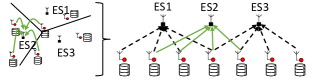
(a) UL OAC.

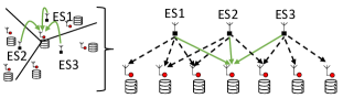
(b) DL OAC.

Figure 1: The interference across the cells (i.e., among the EDs or the ESs) is exploited in both UL and DL for the gradient aggregation.

III Multi-cell Over-the-Air Computation

One of the major advantages of FSK-MV over other state-of-the-art OAC schemes (e.g., OBDA [10]) is that EDs and ESs do not need to utilize the CSI. Also, it does not require precise time-synchronization among the transmitters since the computation with FSK-MV is achieved through a non-coherent detection in the frequency domain. These unique features enable us to extend FSK-MV in a multi-cell environment as the interference in both UL and DL can be exploited for computations: In the UL, the transmitted symbols from an ED superpose not only with the other EDs in the cell, but also with the ones at the neighboring cells. Therefore, the MV calculation at the ESs can exploit the interference from the EDs located at the neighboring cells as illustrated in Figure 1LABEL:sub@subfig:ul_oac. Similarly, in the DL, an ED (e.g., a cell-edge ED) can receive signals from multiple ESs. Hence, the inter-cell interference in the DL can also be used for the MV calculation at the EDs as depicted in Figure 1LABEL:sub@subfig:dl_oac. We discuss the operations at EDs and ESs in the following subsections in detail. The proposed framework is also outlined in Algorithm 1.

Function  multiCellOAC

       for $t=1:T$ do

            

             /* Processing @ EDs

             for $k=1:K$ do

                   Determine $r^{t,{k,m^{+},n^{+}}}_{\rm ED},r^{t,{k,m^{-},n^{-}}}_{\rm ED}$, $\forall i$

                   Detect the MV at the ED, i.e., $v^{t,{k,i}}_{\rm ED}$, $\forall i$

                   Update the model parameter ${\textbf{w}^{(t+1)}_{k}}=\textbf{w}^{(t)}_{k}-\eta\textbf{v}^{t,{k}}_{\rm ED}~{}.$

                   Calculate local gradients based on (6)

                   Calculate $t_{\rm ED}^{t,{k,m^{+},n^{+}}},t_{\rm ED}^{t,{k,m^{-},n^{-}}}$ , $\forall i$

                  

            

             /* Aggregation in the uplink channel

             EDs transmit the corresponding OFDM symbols simultaneously

             ESs receive the superposed OFDM symbols in the uplink

            

             /* Processing @ ESs

             for $s=1:S$ do

                   Determine $r^{t,{s,m^{+},n^{+}}}_{\rm ES},r^{t,{s,m^{-},n^{-}}}_{\rm ES}$, $\forall i$

                   Detect the MV at the ES, i.e., $v^{t,{s,i}}_{\rm ES}$, $\forall i$

                   Calculate $t_{\rm ES}^{t,{s,m^{+},n^{+}}},t_{\rm ES}^{t,{s,m^{-},n}}$, $\forall i$

                  

            

             /* Aggregation in the downlink channel

             ESs transmit the corresponding OFDM symbols simultaneously

             EDs receive the superposed OFDM symbols in the downlink

            

      

Algorithm 1 Multi-cell over-the-air computation

III-A Uplink OAC with FSK-MV

In the UL, the expressions given for the transmitted symbols from the EDs and the superposed symbols at the ES with FSK-MV for a single cell, discussed in Section II-B, also hold in a multi-cell environment for $S>1$. After the $s$th ES calculates the vector $\textbf{v}^{t,{s}}_{\rm ES}$, $\forall s$, the DL OAC starts.

III-B Downlink OAC with FSK-MV

III-B1 Edge Servers - Transmitter

Similar to the UL OAC, we first consider a distinct pairs $(m^{+},n^{+})$ and $(m^{-},n^{-})$ corresponding to the $i$th gradient. Based on the value of $\textbf{v}^{t,{s}}_{\rm ES}$, at the $t$th communication round, the $s$th ES calculates the symbol $t_{\rm ED}^{t,{s,m^{+},n^{+}}}$ and $t_{\rm ED}^{t,{s,m^{-},n^{-}}}$, $\forall i$, as

$$t_{\rm ES}^{t,{s,m^{+},n^{+}}}=\sqrt{E_{\rm s}}s_{\rm ES}^{t,{s,i}}\mathbb{I}\left[{v^{t,{s,i}}_{\rm ES}=1}\right]~{},$$ (10)

and

$$t_{\rm ES}^{t,{s,m^{-},n^{-}}}=\sqrt{E_{\rm s}}s_{\rm ES}^{t,{s,i}}\mathbb{I}\left[{v^{t,{s,i}}_{\rm ES}=-1}\right]~{},$$ (11)

respectively, where $s_{\rm ES}^{t,{s,i}}$ is a random QPSK symbol. All ESs calculate the corresponding OFDM symbols and transmit them simultaneously for DL OAC.

III-B2 Edge Device - Receiver

In the DL, the superposed symbols at the $k$th ED for all $i$ can be expressed as

$$r^{t,{k,m^{+},n^{+}}}_{\rm ED}=\sum_{s=1,\Delta^{t,{s,i}}_{\rm ES}>0}^{S}\sqrt{P^{s,k}_{\rm ES}}h^{t,{s,k,m^{+},n^{+}}}_{\rm DL}t_{\rm ES}^{t,{s,m^{+},n^{+}}}+\omega^{t,{s,m^{+},n^{+}}}_{\rm ED}~{},$$

and

$$r^{t,{k,m^{-},n^{-}}}_{\rm ED}=\sum_{s=1,\Delta^{t,{s,i}}_{\rm ES}<0}^{S}\sqrt{P^{s,k}_{\rm ES}}h^{t,{s,k,m^{-},n^{-}}}_{\rm DL}t_{\rm ES}^{t,{s,m^{-},n^{-}}}+\omega^{t,{s,m^{-},n^{-}}}_{\rm ED}~{}.$$

The energy detector at the $k$th ED then detects the MV for the $i$th gradient as $v^{t,{k,i}}_{\rm ED}=\operatorname{sign}(\Delta^{t,{k,i}}_{\rm ED})$ for $\forall i$, where $\Delta^{t,{k,i}}_{\rm ED}\triangleq|{r^{t,{k,m^{+},n^{+}}}_{\rm ED}}|^{2}-|{r^{t,{k,m^{-},n^{-}}}_{\rm ED}}|^{2}$. Subsequently, the $k$th ED calculates the MV vector, i.e., $\textbf{v}^{t,{k}}_{\rm ED}=[v^{t,{k,1}}_{\rm ED},\hbox to10.00002pt{.\hss.\hss.},v^{t,{k,Q}}_{\rm ED}]^{\rm T}$ and updates its parameters as in (9). Hence, the parameters at the EDs are updated based on the received signals from multiple ESs.

III-C Convergence Analysis

For the convergence analysis, we consider several standard assumptions made in the literature [11, 10]:

Assumption 1 (Bounded loss function).

The loss function has a lower bound for some value $F^{*}$, i.e., $F_{k}(\textbf{w}_{k})\geq F^{*}$, $\forall\textbf{w}_{k}$ [11].

Assumption 2 (Smoothness).

Let ${\textbf{g}}_{k}$ be the gradient of the personalized global loss function $F_{k}(\textbf{w}_{k})$ evaluated at $\textbf{w}_{k}$. For all $\textbf{w}_{k}$ and $\textbf{w}_{k}^{\prime}$, the expression given by

$$\left|F_{k}(\textbf{w}_{k}^{\prime})-(F(\textbf{w}_{k})-{\textbf{g}}_{k}^{\rm T}(\textbf{w}_{k}^{\prime}-\textbf{w}_{k}))\right|\leq\frac{1}{2}\sum_{i=1}^{Q}L_{i}({w}_{i}^{\prime}-{w}_{i})^{2}~{},$$

holds for a non-negative constant vector $\textbf{L}=[L_{1},\hbox to10.00002pt{.\hss.\hss.},L_{Q}]^{\rm T}$.

Assumption 3 (Variance bound).

Assume that the estimated gradient is an unbiased estimate of the true gradient, ${\mathbb{E}}\left[{\tilde{\textbf{g}}}_{k}\right]={\textbf{g}}_{k},~{}\forall k$, and the variance of each component of them is bounded as ${\mathbb{E}}\left[({\tilde{g}}_{k,i}-{g_{k,i}})^{2}\right]\leq\sigma_{i}^{2}/n_{\rm b},~{}\forall k,i$, where ${\bm{\sigma}}=[\sigma_{1},\hbox to10.00002pt{.\hss.\hss.},\sigma_{Q}]^{\rm T}$ is a non-negative constant vector.

Assumption 4 (Unimodal, symmetric gradient noise).

For any given $\textbf{w}_{k}$, the elements of the vector ${\textbf{g}}_{k}$, $\forall k$, has an unimodal distribution that is also symmetric around its mean.

We also assume that the number of EDs that are connected to an ES and the number of ESs that are connected to an ED are fixed and denoted as $K_{\rm c}\leq K$ and $S_{\rm c}\leq S$, respectively (i.e., fixed-connectivity assumption). This assumption is due to the large-scale fading in wireless channels, e.g., an ES can receive the strong signals from the EDs located at its adjacent ESs, but the ones from far cells are likely to be attenuated due to the large link distance. Based on this assumption, let $\mathcal{K}_{s}$ be the set of all EDs that are connected to the $s$th ES and $\mathcal{S}_{k}$ be the set of all ESs that are connected to the $k$th ED, where $|\mathcal{K}_{s}|=K_{\rm c}$, $\forall k$, and $|\mathcal{S}_{k}|=S_{\rm c}$, $\forall s$. We set the received power $P^{s,k}_{\rm ED}=1$ for $k\in{\mathcal{K}_{s}},\forall s$, otherwise $0$, and $P^{s,k}_{\rm ES}=1$ for $s\in{\mathcal{S}_{k}},\forall k$, otherwise $0$. This assumption does not hold for an irregular deployment. Nevertheless, it leads us to provide insight into multi-cell OAC with a tractable analysis since it results in $|{r^{t,{s,m^{+},n^{+}}}_{\rm ES}}|^{2}$ and $|{r^{t,{s,m^{-},n^{-}}}_{\rm ES}}|$ to be exponential random variables with the means $\mu^{+}_{{\rm ES,i}}=E_{\rm s}K^{+}_{s}+\sigma_{\rm ES}^{2}$ and $\mu^{-}_{{\rm ES,i}}=E_{\rm s}K^{-}_{s}+\sigma_{\rm ES}^{2}$, respectively, where $K^{+}_{s}$ and $K^{-}_{s}$ are the cardinalities of the sets $\{{{\bar{g}}_{k,i}^{(t)}=+1}|k\in\mathcal{K}_{s}\}$ and $\{{{\bar{g}}_{k,i}^{(t)}=-1}|k\in\mathcal{K}_{s}\}$, respectively. Also, $|{r^{t,{k,m^{+},n^{+}}}_{\rm ED}}|^{2}$ and $|{r^{t,{k,m^{-},n^{-}}}_{\rm ED}}|^{2}$ become exponential random variables with the means $\mu^{+}_{{\rm ED,i}}=E_{\rm s}S^{+}_{k}+\sigma_{\rm ED}^{2}$ and $\mu^{-}_{{\rm ED,i}}=E_{\rm s}S^{-}_{k}+\sigma_{\rm ED}^{2}$, respectively, where $S^{+}_{k}$ and $S^{-}_{k}$ are the cardinalities of the sets $\{{v^{t,{s,i}}_{\rm ES}=+1}|s\in\mathcal{S}_{k}\}$ and $\{{v^{t,{s,i}}_{\rm ES}=-1}|s\in\mathcal{S}_{k}\}$, respectively. The distributions of $\Delta^{t,{s,i}}_{\rm ES}$ and $\Delta^{t,{k,i}}_{\rm ED}$ can then be calculated as $\Delta^{t,{s,i}}_{\rm ES}\sim f(x,\mu^{+}_{{\rm ES,i}},\mu^{-}_{{\rm ES,i}})$ and $\Delta^{t,{k,i}}_{\rm ED}\sim f(y,\mu^{+}_{{\rm ED,i}},\mu^{-}_{{\rm ED,i}})$ respectively, where $f(x,\mu_{1},\mu_{2})$ is ${{\rm e}^{-\frac{x}{\mu_{1}}}}/{(\mu_{1}+\mu_{2})}$ for $x>0$, and otherwise it is ${{\rm e}^{-\frac{x}{\mu_{2}}}}/{(\mu_{1}+\mu_{2})}$ [15].

Theorem 1.

For $\eta=\frac{1}{T}$ and $n_{\rm b}=\frac{T}{\gamma}$, the convergence rate of multi-cell OAC with FSK-MV in Rayleigh fading channel is

$${\mathbb{E}}\left[\frac{1}{T}{\sum^{T-1}_{t=0}\lVert\textbf{g}_{k}^{(t)}\rVert_{1}}\right]$$

$$\leq\frac{1}{(K-2A){\sqrt{T}}}\left(F_{k}(\textbf{w}^{(0)}_{k})-F^{*}+\frac{1}{2}K\lVert\textbf{L}\rVert_{1}+2\sqrt{\gamma}B\frac{\sqrt{2}}{3}\lVert{\bm{\sigma}}\rVert_{1}\right),$$ (12)

where $\gamma$ is a positive integer, $A$ and $B$ are defined as $A\triangleq\frac{1}{1+\sigma_{\rm ED}^{2}}-B$ and $B\triangleq\frac{S_{\rm c}(\sigma_{\rm ES}^{2}+E_{\rm s}K_{\rm c})}{E_{\rm s}(S_{\rm c}+2\sigma_{\rm ED}^{2})(K_{\rm c}+2\sigma_{\rm ES}^{2})}$, respectively.

Proof:

The proof relies on the strategy used in [11]. By using Assumption 2 and using (9), it can be shown that

$${\mathbb{E}}\left[F_{k}(\textbf{w}^{(t+1)}_{k})-F_{k}(\textbf{w}^{(t)}_{k})\right]\leq-\eta K\lVert\textbf{g}_{k}^{(t)}\rVert_{1}+\frac{{\eta}^{2}}{2}K\lVert\textbf{L}\rVert_{1}$$

$$~{}~{}~{}~{}~{}~{}~{}~{}~{}~{}~{}~{}~{}~{}+2\eta\sum^{K}_{k=1}\sum_{i=1}^{Q}|{g}_{k,i}^{(t)}|\mathbb{P}\left({v^{t,{k,i}}_{\rm ED}\neq\hat{g}^{(t)}_{k,i}}\right)~{},$$

where $\sum^{K}_{k=1}\sum_{i=1}^{Q}|{g}_{k,i}^{(t)}|\mathbb{P}\left({v^{t,{k,i}}_{\rm ED}\neq\hat{g}^{(t)}_{k,i}}\right)$ is the stochasticity-induced error. Let $\hat{g}^{(t)}_{k,i}\triangleq\operatorname{sign}{({g}_{k,i}^{(t)})}$ denote the correct decision. Also, let $Y$ and $Z$ be binomial random variables for the number of ESs and the number of EDs with the correct decision, i.e., $Y\sim B(S_{\rm c},p_{\textrm{y},i})$ and $Z\sim B(K_{\rm c},p_{\textrm{z},i})$, where $p_{\textrm{y},i}$ and $p_{\textrm{z},i}$ denote the success probabilities [11]. The probability $P^{\rm{err}}_{k,i}\triangleq\mathbb{P}\left({v^{t,{k,i}}_{\rm ED}\neq\hat{g}^{(t)}_{k,i}}\right)$ and the success probability $p_{\textrm{y},i}$ can then be written as

$$P^{\rm{err}}_{k,i}=\sum^{S_{\rm c}}_{S^{+}_{k}=1}\mathbb{P}\left({v^{t,{k,i}}_{\rm ED}\neq\hat{g}^{(t)}_{k,i}|Y=S^{+}_{k}}\right)\mathbb{P}\left({Y=S^{+}_{k}}\right)~{},$$ (13)

and

$$p_{\textrm{y},i}= \sum^{K_{\rm c}}_{K^{+}_{s}=1}\mathbb{P}\left({v^{t,{s,i}}_{\rm ES}=\hat{g}^{(t)}_{k,i}|Z=K^{+}_{s}}\right)\mathbb{P}\left({Z=K^{+}_{s}}\right)~{},$$ (14)

respectively. Based on the distributions of $\Delta^{t,{s,i}}_{\rm ES}$ and $\Delta^{t,{k,i}}_{\rm ED}$, we calculate the conditional probabilities in (13) and (14) as

$$\mathbb{P}\left({v^{t,{k,i}}_{\rm ED}\neq\hat{g}^{(t)}_{k,i}|Y=S^{+}_{k}}\right) =\frac{\mu^{-}_{{\rm ED,i}}}{\mu^{+}_{{\rm ED,i}}+\mu^{-}_{{\rm ED,i}}}~{},$$ (15)

and

$$\mathbb{P}\left({v^{t,{s,i}}_{\rm ES}=\hat{g}^{(t)}_{k,i}|Z=K^{+}_{s}}\right) =\frac{\mu^{+}_{{\rm ES,i}}}{\mu^{+}_{{\rm ES,i}}+\mu^{-}_{{\rm ES,i}}}~{},$$ (16)

respectively. By using the definitions of $\mu^{+}_{{\rm ES,i}}$ and $\mu^{-}_{{\rm ES,i}}$ and substituting (16) into (14), we obtain

$$p_{\textrm{y},i} =\sum^{K_{\rm c}}_{K^{+}_{s}=1}\frac{E_{\rm s}K^{+}_{s}+\sigma_{\rm ES}^{2}}{E_{\rm s}K_{\rm c}+2\sigma_{\rm ES}^{2}}\binom{K_{\rm c}}{K^{+}_{s}}p_{\textrm{z},i}^{K^{+}_{s}}{(1-p_{\textrm{z},i})}^{K_{\rm c}-K^{+}_{s}}$$

$$=\frac{E_{\rm s}K_{\rm c}p_{\textrm{z},i}+\sigma_{\rm ES}^{2}}{E_{\rm s}K_{\rm c}+2\sigma_{\rm ES}^{2}}~{}.$$ (17)

By substituting (15) into (13) and using (17), we obtain $P^{\rm{err}}_{i,k}$ as

$$P^{\rm{err}}_{i,k} =\sum^{S_{\rm c}}_{S^{+}_{k}=1}\frac{E_{\rm s}S^{-}_{k}+\sigma_{\rm ED}^{2}}{E_{\rm s}S_{\rm c}+2\sigma_{\rm ED}^{2}}\binom{S_{\rm c}}{S^{+}_{k}}{p_{\textrm{y},i}}^{S^{+}_{k}}{(1-p_{\textrm{y},i})}^{S_{\rm c}-S^{+}_{k}}$$

$$\leq\frac{\sigma_{\rm ED}^{2}+E_{\rm s}S_{\rm c}\left({1-{\frac{\sigma_{\rm ES}^{2}+E_{\rm s}K_{\rm c}\left(1-\frac{\sqrt{2}}{3S}\right)}{E_{\rm s}K_{\rm c}+2\sigma_{\rm ES}^{2}}}}\right)}{E_{\rm s}S_{\rm c}+2\sigma_{\rm ED}^{2}}~{},$$ (18)

for $S\triangleq{|{g}_{k,i}^{(t)}|}/{\frac{\sigma_{i}^{2}}{\sqrt{n_{\rm b}}}}$. Accordingly, an upper bound for the stochasticity-induced error can be obtained as follows:

$$\sum^{K}_{k=1}\sum_{i=1}^{Q}|{g}_{k,i}^{(t)}|P^{\rm{err}}_{k,i}\leq A\lVert\textbf{g}_{k}^{(t)}\rVert_{1}+B\frac{\sqrt{2}}{3\sqrt{n_{\rm b}}}\lVert{\bm{\sigma}}\rVert_{1},$$ (19)

where $A$ and $B$ are defined in Theorem 1. By considering Assumption 1, an upper bound can then be obtained as follows:

$$F^{*}-F_{k}(\textbf{w}^{(0)}_{k})$$

$$\leq{\mathbb{E}}\left[\sum^{T-1}_{t=0}-\eta K\lVert\textbf{g}_{k}^{(t)}\rVert_{1}+\frac{{\eta}^{2}}{2}K\lVert\textbf{L}\rVert_{1}+2\eta\sum^{K}_{k=1}\sum_{i=1}^{Q}|{g}_{k,i}^{(t)}|P^{\rm{err}}_{k,i}\right]$$

$$={\mathbb{E}}\left[\sum^{T-1}_{t=0}-\eta(K-2A)\lVert\textbf{g}_{k}^{(t)}\rVert_{1}+\frac{{\eta}^{2}}{2}K\lVert\textbf{L}\rVert_{1}+2\eta B\frac{\sqrt{2}}{3\sqrt{n_{\rm b}}}\lVert{\bm{\sigma}}\rVert_{1}\right].$$

Finally, by rearranging terms of the above equation and considering $\eta=\frac{1}{T}$ and $n_{\rm b}=\frac{T}{\gamma}$, (12) can be reached. ∎

IV Numerical Results

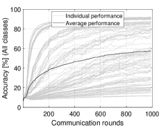
(a) All classes, homogeneous data.

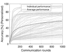
(b) Personalized, heterogeneous data.

Figure 2: Test accuracy - communication round for a single cell ($|\mathcal{G}|=30000$).

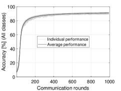
(a) All classes, homogeneous data.

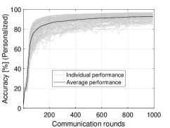
(b) Personalized, heterogeneous data.

Figure 3: Test accuracy - communication round for multiple cells ($|\mathcal{G}|=30000$).

To numerically evaluate multi-cell OAC, we consider the learning task of handwritten-digit recognition over an hexagonal tessellation with $77$ cells, i.e., $S=77$ ESs, where $K=120$ EDs are located at the cell edge and the distance between two adjacent ESs is $50$ meters (see Figure 6). Under this specific deployment, $K_{\rm c}$ and $S_{\rm c}$ are approximately $6$ and $3$, respectively. Our evaluation is limited to FSK-MV since it is the only scheme that allows both OAC in both UL and DL, to the best of our knowledge. For the large-scale channel model, we assume that the path loss exponent is $\alpha=4$ and the UL and DL SNRs are set to $20$ dB for $r_{\rm UL}=r_{\rm DL}=25/\cos(\pi/6)$. For the fading channel, we consider ITU Extended Pedestrian A (EPA) with no mobility in both UL and DL and capture the long-term channel variations by regenerating the channels between the ESs and the EDs independently for each communication round. In this study, we also assume that the UL and DL channel realizations are independent of each other. The subcarrier spacing and the CP duration are set to $15$ kHz and $4.7$ $\mu$s, respectively. We use $M=1200$ subcarriers (i.e., the signal bandwidth is $18$ MHz). Therefore, $T_{\rm sync}$ can be calculated as $55.6$ ns.

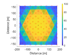
(a) All classes, homogeneous data.

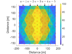
(b) Personalized, heterogeneous data.

Figure 4: Distribution of the test accuracy for a single cell ($\times$: ES, $\circ$: ED, Blue: Low test accuracy, Yellow: High test accuracy, $|\mathcal{G}|=30000$).

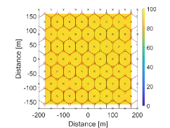
(a) All classes, homogeneous data.

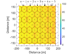
(b) Personalized, heterogeneous data.

Figure 5: Distribution of the test accuracy for multiple cells ($\times$: ES, $\circ$: ED, Blue: Low test accuracy, Yellow: High test accuracy, $|\mathcal{G}|=30000$).

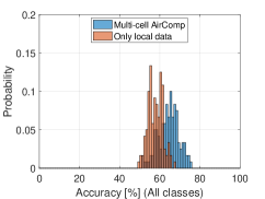
(a) All classes, homogeneous data.

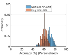
(b) Personalized, heterogeneous data.

Figure 6: Test accuracy with multi-cell FL with the proposed OAC or the training based on only local data after 400 iterations ($|\mathcal{G}|=5000$).

For the local data at the EDs, we use the MNIST database that contains labeled handwritten-digit images size of $28\times 28$ from digit 0 to digit 9. We consider both homogeneous data and heterogeneous data distribution in the cell. To prepare the data, we first choose $|\mathcal{G}|\in\{5000,30000\}$ training images from the database, where each digit has the identical number of images. For the scenario with the homogeneous data distribution, each local dataset has approximately an equal number of distinct images for each digit. For the scenario with the heterogeneous data distribution, we assume that the distribution of the images depends on the locations of the EDs. To this end, we divide the area into 5 identical parallel areas, where the EDs located in the $a$th area have the data samples with the labels $\{a-1,a,1+a,2+a,3+a,4+a\}$ for $a\in\{1,\hbox to10.00002pt{.\hss.\hss.},5\}$ (see Figure 6LABEL:sub@subfig:dep_mc_20_accPer_niid). Hence, the availability of the labels gradually changes. The model at EDs is based on a convolution neural network (CNN) described in [15]. It has $Q=123090$ learnable parameters, which corresponds to $N=206$ OFDM symbols in both UL and DL, respectively. The learning rate is $0.0001$. The batch size $n_{\rm b}$ is $16$. For the test accuracy calculation, we use $10000$ test samples available in the MNIST database. For the personalized test accuracy, we test the models based on only the classes available at the ED’s local dataset.

In Figure 3, we evaluate the test accuracy versus communication round in a single cell under homogeneous and heterogeneous data distributions. When there is only a single ES for the aggregation and the data distribution in the area is homogeneous, only a few number of EDs obtain a high test accuracy, while a majority of EDs fails to recognize the digits as shown in Figure 3LABEL:sub@subfig:acc_sc_20_acc_iid. The personalized test accuracy results for heterogeneous data distribution in Figure 3LABEL:sub@subfig:accPer_sc_20_acc_niid are also low (i.e., the EDs cannot even learn the classes that are available at their local datasets). In Figure 3, we consider multi-cell scenario. When the data distribution is homogeneous, all EDs result in higher test accuracy results as demonstrated in Figure 3LABEL:sub@subfig:acc_mc_20_acc_iid. The personalized test accuracy is also high for the heterogeneous data distribution as can be seen in Figure 3LABEL:sub@subfig:accPer_mc_20_acc_niid. This demonstrates that EDs learn to classify the labels while being harmonious with other EDs in the wireless network with the proposed OAC framework. Figure 3 shows that the convergence for this specific learning task can be achieved approximately after $200$ rounds. Thus, the amount of consumed time-frequency resources can be calculated as $2\times(66.7+4.7)\mu s\times 206\times 200=5.88$ seconds over $18$ MHz, respectively.

In Figure 6LABEL:sub@subfig:dep_sc_20_acc_iid and Figure 6LABEL:sub@subfig:dep_sc_20_accPer_niid, we show the distribution of the test accuracy in the area. The single-cell OAC suffers from path loss: The far EDs’ votes cannot contribute the MV decision in the UL. Similarly, the ES’s signal is not strong at the far EDs in the DL. Therefore, only nearby EDs get benefit from the FEEL and the ones have similar data distribution. On the other hand, multi-cell OAC yields almost a uniform distribution for both homogeneous and heterogeneous data as it can be seen in Figure 6LABEL:sub@subfig:dep_mc_20_acc_iid and Figure 6LABEL:sub@subfig:dep_mc_20_accPer_niid, respectively.

In Figure 6, we evaluate if the proposed OAC method is superior to the case where each ED performs the training based on its own local data. To this end, we intentionally reduce $|\mathcal{G}|$ to $5000$ and set $\eta=0.01$ to demonstrate if the EDs are able to leverage the data at the neighbouring EDs through FEEL. We plot the histogram of the test accuracy after $400$ iterations for both cases. The results show that, in both homogeneous and heterogeneous data distributions, the proposed concept improves the average test accuracy based on all classes and personalized test accuracy in this scenario.

V Concluding Remarks

In this paper, we present a multi-cell OAC framework where the aggregations occur in both UL and DL across multiple cells through a non-coherent OAC scheme, i.e., FSK-MV. We also prove the convergence of FEEL under a fixed-connectivity assumption. Finally, we evaluate the test accuracy of the multi-cell OAC by comparing it with the one for a single-cell scenario for homogeneous and heterogeneous data distributions. Our numerical results show that the proposed approach is a promising solution to achieve a high-test accuracy at the EDs by exploiting the interference among multiple cells. In this study, our analysis is based on regular tessellation. For an irregular deployment, the interference distributions in UL and DL need to be considered for the convergence analysis, which will be investigated in future work.

References

• [1] B. Nazer and M. Gastpar, “Computation over multiple-access channels,” IEEE Trans. Inf. Theory, vol. 53, no. 10, pp. 3498–3516, Oct. 2007.
• [2] M. Goldenbaum, H. Boche, and S. Stańczak, “Harnessing interference for analog function computation in wireless sensor networks,” IEEE Trans. Signal Process., vol. 61, no. 20, pp. 4893–4906, Oct. 2013.
• [3] M. Tang, S. Cai, and V. K. N. Lau, “Remote state estimation with asynchronous mission-critical IoT sensors,” IEEE Journal on Selected Areas in Communications, vol. 39, no. 3, pp. 835–850, Aug. 2021.
• [4] L. Chen, X. Qin, and G. Wei, “A uniform-forcing transceiver design for over-the-air function computation,” IEEE Wireless Communications Letters, vol. 7, no. 6, pp. 942–945, May 2018.
• [5] T. Gafni, N. Shlezinger, K. Cohen, Y. C. Eldar, and H. V. Poor, “Federated learning: A signal processing perspective,” 2021. [Online]. Available: arXiv:2103.17150
• [6] M. Chen, D. Gündüz, K. Huang, W. Saad, M. Bennis, A. V. Feljan, and H. Vincent Poor, “Distributed learning in wireless networks: Recent progress and future challenges,” IEEE J. Sel. Areas Commun., pp. 1–26, 2021.
• [7] L. Liu, J. Zhang, S. Song, and K. B. Letaief, “Client-edge-cloud hierarchical federated learning,” in ICC 2020 - 2020 IEEE International Conference on Communications (ICC), 2020, pp. 1–6.
• [8] G. Zhu, Y. Wang, and K. Huang, “Broadband analog aggregation for low-latency federated edge learning,” IEEE Trans. Wireless Commun., vol. 19, no. 1, pp. 491–506, Jan. 2020.
• [9] M. M. Amiri and D. Gündüz, “Federated learning over wireless fading channels,” IEEE Trans. Wireless Commun., vol. 19, no. 5, pp. 3546–3557, Feb. 2020.
• [10] G. Zhu, Y. Du, D. Gündüz, and K. Huang, “One-bit over-the-air aggregation for communication-efficient federated edge learning: Design and convergence analysis,” IEEE Trans. Wireless Commun., vol. 20, no. 3, pp. 2120–2135, Nov. 2021.
• [11] J. Bernstein, Y.-X. Wang, K. Azizzadenesheli, and A. Anandkumar, “signSGD: Compressed optimisation for non-convex problems,” in Proc. in International Conference on Machine Learning, vol. 80.   Proceedings of Machine Learning Research, 10–15 Jul 2018, pp. 560–569.
• [12] L. Su and V. K. N. Lau, “Hierarchical federated learning for hybrid data partitioning across multitype sensors,” IEEE Internet of Things Journal, vol. 8, no. 13, pp. 10 922–10 939, Jan. 2021.
• [13] K. Yang, T. Jiang, Y. Shi, and Z. Ding, “Federated learning via over-the-air computation,” IEEE Trans. Wireless Commun., vol. 19, no. 3, pp. 2022–2035, 2020.
• [14] M. M. Amiria, T. M. Duman, D. Gündüz, S. R. Kulkarni, and H. Vincent Poor, “Collaborative machine learning at the wireless edge with blind transmitters,” IEEE Trans. Wireless Commun., pp. 1–1, Mar 2021.
• [15] A. Şahin, B. Everette, and S. Hoque, “Distributed learning over a wireless network with FSK-based majority vote,” in Proc. IEEE International Conference on Advanced Communication Technologies and Networking (CommNet), Dec. 2021, pp. 1–9.
• [16] ——, “Over-the-air computation with DFT-spread OFDM for federated edge learning,” in Proc. IEEE Wireless Communications and Networking Conference (WCNC), Apr. 2022, pp. 1–6.