Fine-grained Differentiable Physics: A Yarn-level Model for Fabrics

Abstract

Differentiable physics modeling combines physics models with gradient-based learning to provide model explicability and data efficiency. It has been used to learn dynamics, solve inverse problems and facilitate design, and is at its inception of impact. Current successes have concentrated on general physics models such as rigid bodies, deformable sheets, etc, assuming relatively simple structures and forces. Their granularity is intrinsically coarse and therefore incapable of modelling complex physical phenomena. Fine-grained models are still to be developed to incorporate sophisticated material structures and force interactions with gradient-based learning. Following this motivation, we propose a new differentiable fabrics model for composite materials such as cloths, where we dive into the granularity of yarns and model individual yarn physics and yarn-to-yarn interactions. To this end, we propose several differentiable forces, whose counterparts in empirical physics are indifferentiable, to facilitate gradient-based learning. These forces, albeit applied to cloths, are ubiquitous in various physical systems. Through comprehensive evaluation and comparison, we demonstrate our model’s explicability in learning meaningful physical parameters, versatility in incorporating complex physical structures and heterogeneous materials, data-efficiency in learning, and high-fidelity in capturing subtle dynamics. Code is available in: https://github.com/realcrane/Fine-grained-Differentiable-Physics-A-Yarn-level-Model-for-Fabrics.git

1 Introduction

Differentiable physics models (DPMs) have recently spiked interests, e.g. rigid bodies (Heiden et al., 2020), cloth (Liang et al., 2019), and soft bodies (Hu et al., 2019). The essence of DPMs is making physics models differentiable, so that gradient-based learning can be used to make systems adhere strictly to physical dynamics. This is realized via back-propagation through a series of observed actions, where the system can quickly learn the underlying dynamics. While enjoying neural networks’ capability of modeling arbitrary non-linearity, DPMs also improve the model explicability as the learnable model parameters bear physical meanings. As a result, such models provide a new avenue for many applications such as inverse problems, e.g. estimating the mass of a moving rigid body (de Avila Belbute-Peres et al., 2018b), and control, e.g. learning to shake a bottle to shape the fluid in it (Li et al., 2019).

Early research attempted to model simple and general physical systems such as rigid bodies (de Avila Belbute-Peres et al., 2018b), followed by a range of systems including deformable objects (Li et al., 2019), cloth (Liang et al., 2019), contacts (Zhong et al., 2021), etc. However, existing models are only generally-purposed which do not consider complex structures/topologies and force interactions. Taking cloth (i.e. fabrics) as an example, existing models (Liang et al., 2019; Li et al., 2019) can learn general cloth dynamics, but only when the cloth is relative simple and homogeneous. Recent research (Wang et al., 2020) has started to explore articulated systems but the model capacity is insufficient to capture the full dynamics of complex systems such as fabrics. Since real-world physical systems (e.g. materials in engineering) often have sophisticated structures and consist of heterogeneous materials, we argue that it is crucial to design fine-grained DPMs, for differentiable physics to be truly applicable and meaningful to real-world applications.

This paper focuses on fabrics which are composite materials consisting of basic slim units arranged in different patterns. A common example in fabrics is woven cloth which is made from yarns of different materials (silk, cotton, nylon, etc.) interlaced in various patterns (e.g. plain, satin, twill). Fabrics present new challenges in differentiable modeling. First, the dynamics heterogeneity caused by material and structural diversity needs to be incorporated into modeling, which is especially crucial for solving inverse problems where the physical properties are learned from data. General DPMs without sufficient granularity can only approximate the dynamics and are unable to learn meaningful parameters. Second, certain forces that are essential for fabrics dynamics are indifferentiable. One such example is friction. The standard Coulomb model for rigid bodies has been made differentiable recently (de Avila Belbute-Peres et al., 2018b; Zhong et al., 2021). However, it is overly simplified for fabrics because the yarn-to-yarn friction shows richer dynamics (Zhou et al., 2017) that is beyond the capacity of existing methods. Further, the contact modeling together with friction requires new treatments that previous methods did not have to consider.

To overcome these challenges, we propose a new DPM for fabrics at a more fine-grained level and apply it to cloth modeling. Unlike general DPMs, we start with a fine-grained yarn-level model. By modeling each yarn individually, we provide the capacity of modeling fabrics with mixed yarns and different woven patterns, which could not be handled previously. To facilitate gradient-based learning, we propose new differentiable forces on/between yarns, including contact, friction and shear. Finally, we incorporate implicit Euler and implicit differentiation to compute gradients induced by an optimization problem embedded in the simulation.

To our best knowledge, our model is the first differentiable physics model which provides sufficient granularity for heterogeneous materials such as fabrics. We comprehensively evaluate its learning capability, data efficiency and fidelity. Since there is no similar model, we compare our model with the most similar work (Liang et al., 2019) and traditional Bayesian optimization on inverse problems. We also compare our work on control learning with popular Reinforcement Learning methods. We show that our model is more explicable, has higher data efficiency, generates more accurate predictions in inverse problem and control learning respectively.

2 Related work

Differentiable physics simulator. A differentiable simulator integrates differentiable physics engine into the forward and backward propagation of learning. As a strong inductive bias, these simulation engines increase data efficiency and learning accuracy over gradient-free models. Due to these advantages, differentiable simulation demonstrates superiority in a number of problem domains such as inverse problem, robot control and motion planning. The early works focused initially on simple rigid bodies (de Avila Belbute-Peres et al., 2018a; Degrave et al., 2019) and later simulation of high degrees of freedom systems, such as fluids (Schenck & Fox, 2018), elastic bodies (Hu et al., 2019; Huang et al., 2021), and cloth (Liang et al., 2019). More recently, Jatavallabhula et al. (2021) introduced an end-to-end differentiable simulator that can learn from images by combining differentiable rendering and differentiable simulation. Comparatively, we explore fine-grained DPMs for composite materials, which leads to new challenges in differentiable modeling.

Cloth simulation. Cloth simulation initially appeared in textile engineering and was then introduced to computer graphics (Long et al., 2011). Cloth has been modeled as particle systems (Breen et al., 1992), mass-spring systems (Provot et al., 1995), and continuum (Narain et al., 2012). Kaldor et al. (2008) proposed a yarn-level knit cloth simulator and found that cloth microstructures have a considerable influence on cloth dynamics. Since then the cloth simulation community has shifted the focus to yarn-level cloth simulation. Based on the objectives, the recent research can be classified to increasing efficiency (Kaldor et al., 2010; Cirio et al., 2016), combining continuum models and yarn-level models (Casafranca et al., 2020; Sperl et al., 2020), introducing woven cloth simulation (Cirio et al., 2014), and optimizations (Pizana et al., 2020; Sánchez-Banderas et al., 2020). Our work is orthogonal to these papers in that we introduce a new methodology to incorporate differentiable physics into yarn-level models.

Machine learning and cloth simulation. Machine learning was initially introduced to cloth simulation to make data-driven simulators, which have inherent advantages in simulation efficiency over physical-based methods (James & Fatahalian, 2003; Kim & Vendrovsky, 2008), and can help improve fidelity (Lahner et al., 2018). In parallel, machine learning has been applied to discover the physical properties from visual information. Bouman et al. (2013) proposed a linear regression model for evaluating cloth density and stiffness from the dynamics of wind-blown cloth. Yang et al. (2017b) introduced a neural network for classifying cloths based on how their dynamics are affected by stretching and bending stiffness. Rasheed et al. (2020) proposed a model for estimating the friction coefficient between cloth and other objects. By combining physically-based cloth simulators and neural networks, Runia et al. (2020) estimated cloth parameters by training neural networks to adjust a simulator’s parameters so that the simulated cloth mimics the observed one in videos. Different from these gradient-free models, Liang et al. (2019) and Li et al. (2021) proposed sheet-level differentiable cloth models that can be used to estimate cloth parameters. In this work, we dive into fine-grained physics and propose a new yarn-level differentiable fabrics model which can be embedded into deep neural networks as a layer.

3 Methodology

Since cloth is employed as an application in this paper, we use the terms ‘cloth’ and ‘fabric’ interchangeably. We first explain the cloth representation (Sec. 3.1) and the (physics) system equation for simulation (Sec. 3.2). Then we present our new force models (Sec. 3.3), and how we solve the system equation to enable back-propagation (Sec. 3.4).

3.1 Cloth representation

Similar to Cirio et al. (2014), our cloth consists of two perpendicular groups of parallel yarns named warps and wefts. Every pair of warp and weft are in contact with each other at one crossing node (Figure 1), with a persistent contact. We employ an Eulerian-on-Lagrangian discretization (Sueda et al., 2011), and denote the Degrees of Freedom (DoFs) of every crossing node as $\mathbf{q}_{i}\equiv(\mathbf{x}_{i},u_{i},v_{i})$. $\mathbf{x}_{i}\in\mathbb{R}^{3}$ is the Lagrangian coordinates indicating spatial locations and $(u_{i},v_{i})$ is the Eulerian coordinates indicating sliding movements between yarns. The end points of yarns do not contact with other yarns and hence they are treated as special crossing nodes that have no Eulerian terms, i.e. $\mathbf{q}_{j}\equiv\mathbf{x}_{i}$. Therefore, on a $r(rows)\times c(columns)$ cloth, there are $(r-2)\times(c-2)$ crossing nodes with five DoFs and $2r+2c-4$ crossing nodes with three DoFs. Every two neighboring crossing nodes on the same warp/weft delimit a warp/weft segment. A warp segment with end points $\mathbf{q}_{0}$ and $\mathbf{q}_{1}$ is denoted as $\mathbf{[q_{0},q_{1}]}$ and its position is $(\mathbf{x}_{0},\mathbf{x}_{1},u_{0},u_{1})$ (Figure 1). This way, a woven cloth is discretized into crossing nodes and segments which are the primitive units of the cloth. Every segment is assumed to be straight so that linear interpolation can be employed on the segment, i.e. the spatial location of a point in the segment $\mathbf{[q_{0},q_{1}]}$ is $\mathbf{x}(u)=\frac{u-u_{0}}{\Delta u}\mathbf{x}_{0}+\frac{u_{1}-u}{\Delta u}\mathbf{x}_{1}$, where $u$ is the point’s position in Eulerian coordinates and $\Delta u=u_{1}-u_{0}$ is the crossing nodes distance in Eulerian coordinates. We use $L$ to denote the rest length of the yarn segment and $R$ to denote the yarn radius.

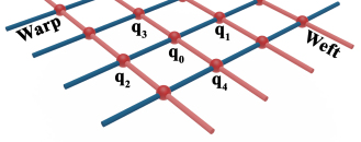
Figure 1: Blue and red rods denote warps and wefts respectively. $\mathbf{q}$s are the crossing nodes.

3.2 System equation for simulation

A cloth’s state at time $t$, $\mathcal{S}_{(t)}=\{\mathcal{Q}_{(t)},\dot{\mathcal{Q}}_{(t)}\}$, includes all the crossing node DoFs $\mathcal{Q}=\{\mathbf{q}_{i}|i=1,2,\dots,N\}$ and their velocities $\dot{\mathcal{Q}}=\{\dot{\mathbf{q}}_{i}|i=1,2,\dots,N\}$, where $N$ is the number of crossing nodes. Knowing the state, we can calculate the internal and external forces:

$$\mathbf{F}=\mathbf{M}\ddot{\mathbf{q}}=\frac{\partial T}{\partial\mathbf{q}}-\frac{\partial V}{\partial\mathbf{q}}-\dot{\mathbf{M}}\dot{\mathbf{q}}$$ (1)

where $\mathbf{q}$, $\dot{\mathbf{q}}$, and $\ddot{\mathbf{q}}$ are the general position, velocity, and acceleration respectively, with a dimension $l=3\times r\times c+2\times(r-2)\times(c-2)$. $\mathbf{M}\in\mathbb{R}^{l\times l}$ is the general mass matrix. The model assumes mass is distributed homogeneously. $T$ and $V$ are the kinetic and potential energy. As force is related to the partial derivative of energy with respect to position, the right hand terms in Eq. 1 are inertia, conservative forces, and part of the time derivative of $\mathbf{M}\dot{\mathbf{q}}$. Non-conservative forces are added to the right side of the equation. Section 3.3 gives the details of all the forces considered in our model. Using implicit Euler (Baraff & Witkin, 1998), we can derive the system equation for simulation:

$$\left(\mathbf{M}-\frac{\partial\mathbf{F}_{(t)}}{\partial\mathbf{q}}h^{2}-\frac{\partial\mathbf{F}_{(t)}}{\partial\dot{\mathbf{q}}}h\right)\dot{\mathbf{q}}_{(t+1)}=h\left(\mathbf{F}_{(t)}-\frac{\partial\mathbf{F}_{(t)}}{\partial\dot{\mathbf{q}}}\dot{\mathbf{q}}_{(t)}\right)+\mathbf{M}\dot{\mathbf{q}}_{(t)}$$ (2)

where the subscript in brackets $t$ indicates the associate variable at time $t$. Detailed deduction is in Appendix.

3.3 Force models

To simulate cloth, we need to compute the inertia, internal and external forces in Equation 2. Inertia is the derivative of kinetic energy with respect to node positions. As woven cloths are interlaced yarns, the internal forces can be further classified into 1) forces caused by yarn deformation and 2) forces resulting from yarn-to-yarn interactions. We treat each yarn as an elastic rod that can generate elastic energy, including stretching and bending (Jawed et al., 2018), ignoring the twisting due to its triviality in cloth dynamics  (Cirio et al., 2014). The elastic energy is $V^{e}=V^{s}+V^{b}$, where $V^{s}$ and $V^{b}$ are the stretching and bending energy respectively. The yarn-to-yarn interaction forces include friction, shear, and parallel yarn collisions. We refer the reader to Appendix for the inertia, stretching, and bending force as it is straightforward to show that they are differentiable.

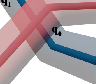
Figure 2: Compression force on $\mathbf{q}_{0}$ along normal $\mathbf{n}$ at $\mathbf{q}_{0}$.

Yarn-to-yarn contact. While the aforementioned forces are differentiable, the yarn-to-yarn forces are not. Existing differentiable contact models mainly correct after-contact positions and velocities (de Avila Belbute-Peres et al., 2018b; Liang et al., 2019; Zhong et al., 2021) via (multiple) optimization solves, which is too simplistic for fabrics. Yarn-to-yarn contact has its unique features. It is relatively sticky and often has small relative velocities. We need a contact model that reflects this and leads to a differentiable contact force which affects the friction/shear. The contact force is a combination of the stretching $\mathbf{F}_{s}$ and bending forces $\mathbf{F}_{b}$ at every crossing node along the contact normal $\mathbf{n}$. We assume no-slip contact and compute the contact force by:

$$F_{n}=\mbox{ReLU}(\frac{1}{2}\mathbf{n}^{\top}(\mathbf{F}_{s}^{u}+\mathbf{F}_{b}^{u}-\mathbf{F}_{s}^{v}-\mathbf{F}_{b}^{v}))$$ (3)

where $u$ and $v$ represent the forces from warp and weft segments. The rectified linear unit (ReLU) ensures the non-negativity of the contact force. The normal $\mathbf{n}$, from warp to weft yarn (Fig. 2), is approximated by the normal of the best-fit plane of $\mathbf{q_{0}}$-$\mathbf{q_{4}}$.

Friction. The friction between warps and wefts prohibits relative movements, which is crucial to the overall dynamics of the fabric. In differentiable physics, contacts under simple settings have been modeled, such as the standard Coulomb model for kinetic friction (Zhong et al., 2021). But this is insufficient for our purpose for two reasons. First, the static friction plays a key role in stick-slip behaviours of yarns (Zhou et al., 2017) and needs to be modeled. Second, the standard Coulomb friction model is a piece-wise function, which is intrinsically indifferentiable at the static-to-kinetic transition point. Therefore, we need a new differentiable friction model.

The low relative speed between yarns is a special situation where the static-to-kinetic transition could actually be continuous (as opposed to the Coulomb model), experimentally shown by Stribeck (Stribeck, 1902). This indicates that a continuous and differentiable model has the potential to be more accurate for yarns than the widely used Coulomb model. Further, the breakaway force causing the static-to-kinetic transition depends on the rate of the external force (Johannes et al., 1973), and the nonlinear stick-slip behavior is related to self-excited vibrations before transition (Awrejcewicz, 1988). Inspired by the above research, we propose a new differentiable yarn-to-yarn friction model (Figure 3):

$$F_{Slide}=-\Big{(}\frac{k_{f}\delta u-K(\delta u)\mu F_{n}}{2}K(\mu F_{n}-F_{u})+\frac{k_{f}\delta u+K(\delta u)\mu F_{n}}{2}\Big{)}-d_{f}\dot{u}_{0}$$ (4)

where $\delta u=u_{0}-\bar{u}_{0}$ and $K(x)=\tanh(px)$. $\bar{u}_{0}$ is the anchor position when there is no relative movement between the warp and the weft segment, $\mu$ is the friction coefficient, and $F_{u}$ is the external force. We introduce a hyperparameter $p$ to control the conversion speed between static and kinetic friction. To understand Equation 4, there are three situations: $F_{u}=0$ (no external force), $0\leq F_{u}\leq\mu F_{n}$ (static friction), and $F_{u}>\mu F_{n}$ (kinetic friction). When $F_{u}=0$, $\delta u=0$, $K(\mu F_{n}-F_{u})=1$ and the speed $\dot{u}_{0}=0$, so $F_{Slide}=0$; when $0\leq F_{u}\leq\mu F_{n}$, we allow a small displacement $\delta u$ to mimic the self-excited vibration in static friction, governed by a Hooke’s spring $k_{f}\delta u$ with stiffness $k_{f}$. When $F_{u}$ is small, i.e. $K(\mu F_{n}-F_{u})$ is close to 1, $F_{Slide}\approx-k_{f}\delta u-d_{f}\dot{u}_{0}$ where $d_{f}$ is a damping coefficient. $F_{Slide}$ is mainly the static friction minus a small damping term (as $\dot{u}_{0}$ is small). Due to the time discretization in simulation, the spring force has a delayed response which causes small-range vibrations. When $K(\mu F_{n}-F_{u})$ starts to decrease to 0 and the breakaway force is achieved $F_{u}=\mu F_{n}$, $F_{Slide}=-\frac{k_{f}\delta u+K(\delta u)\mu F_{n}}{2}-d_{f}\dot{u}_{0}$ and $\frac{k_{f}\delta u+K(\delta u)\mu F_{n}}{2}$ is the average of the spring force and the maximum static friction. Finally when $F_{u}>\mu F_{n}$, $K(\mu F_{n}-F_{u})$ quickly becomes -1 and $K(\delta u)$ becomes 1 as $\delta u$ increases. Then $F_{Slide}=-\mu F_{n}-d_{f}\dot{u}_{0}$, which is the kinetic friction minus damping. Fig. 3 shows our friction can closely approximate the Stribeck effect while maintaining differentiability, as opposed to the indifferentiable Coulomb model. Also, it incorporates self-excited vibrations within $F_{Slide}\in[-F_{k},F_{k}]$ which is when $0\leq F_{u}\leq\mu F_{n}$.

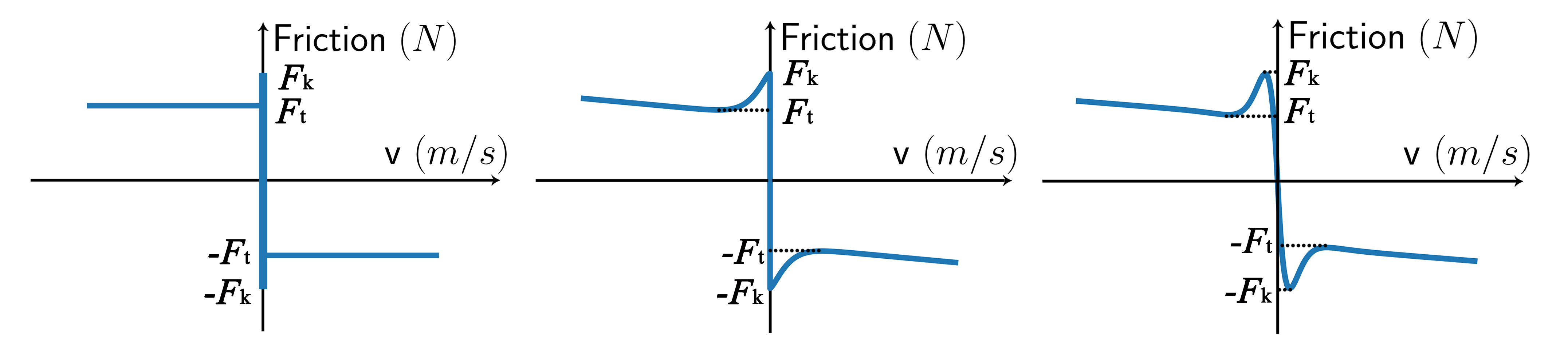
Figure 3: $F_{k}$ and $F_{t}$ are the static and kinetic friction. Coulomb model (left) is an indifferentiable multi-value function. Stribeck effect (middle) is empirically observed (Stribeck, 1902). Our model (right) incorporates the Stribeck effect and also simulates self-excited vibrations around $\mathsf{v}=0$.

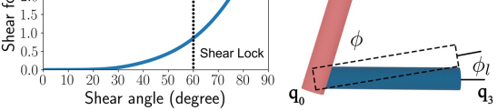
Figure 4: Shear force strength vs shear angle $\bar{\phi}-\phi$, (left) and graphical illustration (right).

Shear. A shear force is generated when there is relative rotation between a warp and a weft at a crossing node (Parsons et al., 2010), which increases non-linearly when the shear angle increases (Mohammed et al., 2000; Peng et al., 2004; Cao et al., 2008). Previous differential models do not consider this type of forces. Therefore, we propose a new differentiable shear model. There are different stages when the shear angle increases (King et al., 2005). The shear force first grows almost linearly initially, then ‘shear lock’ is triggered (Wang et al., 1999) when the angle passes a threshold and the shear force starts to increase exponentially as the angle increases, producing highly non-linear behaviors. We therefore define the shear energy as a function of the shear angle $\bar{\phi}-\phi$ (Figure 4): $\frac{1}{2}k_{s}L(\phi-\bar{\phi})^{2}$, where $\bar{\phi}=\frac{\uppi}{2}$ is the rest shear angle. $k_{s}=S\uppi R^{2}(1+F_{n})$ is the shear stiffness and $S$ is the shear modulus. We embed the ‘shear lock’ by boosting $k_{s}$ exponentially with $\gamma=(\sqrt{2L^{2}}-2\sin\frac{\phi}{2}L)/R$ as long as it stays smaller than the lock threshold $\phi_{l}=2\arcsin{\frac{R}{L}}$: $k_{s}$ equals to $S\uppi R^{2}(1+F_{n})$ if $\phi>\phi_{l}$; and $S\uppi R^{2}(1+F_{n})\gamma^{c}$ otherwise, where $c$ controls the increase rate of $k_{s}$ with respect to $\phi$ when ‘shear lock’ occurs. Although $k_{s}$ has discontinuities within $[0,\frac{\phi}{2}]$, our new shear stiffness can be defined as:

$$k_{s}=\frac{1}{2}(F_{n}+1)S\uppi R^{2}\Bigg{(}(1+\gamma^{c})+(1-\gamma^{c})\tanh\left(\frac{\bar{\phi}^{5}(\phi-\phi_{l})}{(\phi(\phi-\phi_{l})(\phi-\bar{\phi}))^{2}+\bar{\phi}^{4}\sigma^{2}}\right)\Bigg{)}$$ (5)

where $\sigma$ governs the transition smoothness between lock and no-lock. The smaller the $\sigma$ is, the smoother the transition is. The shear force (Figure 4) derivation is in Appendix.

Yarn-to-yarn collision. The last internal force is the yarn-to-yarn collisions between parallel yarns. Although it is theoretically possible to use an existing approach (de Avila Belbute-Peres et al., 2018b; Liang et al., 2019), it would require forming an optimization for all segments and therefore become prohibitively slow. Therefore, we introduce a new penalty energy, defined as a function of the nodes’ distance in Eulerian coordinates for a warp segment $[\mathbf{q}_{0},\mathbf{q}_{1}]$ (similar for a weft segment): $V_{0,1}=\frac{1}{2}k_{c}L(\mbox{ReLU}(d-\Delta u))^{2}$ where $d=4R$ or $2R$ which is elaborated in Appendix.

External forces and collisions. Without loss of generality, we consider two external forces: gravity and wind force. Their impacts can be modeled by defining proper potential energies. Finally, after calculating all forces, the resultant force at every crossing node is the combined force of all segments that connect to that node. The cloth is simulated by solving Equation 2. We use bounding volume hierarchy (Tang et al., 2010) with continuous collision detection and non-rigid impact zones (Harmon et al., 2008) to compute collision. Similar to Liang et al. (2019); Wang et al. (2020), we form an optimization problem for continuous collision. Details can be found in Appendix.

3.4 Derivatives of the simulator

Now we have a fully differentiable simulator with parameters $\bm{\omega}$. The $\bm{\omega}$ is the cloth physical parameters (stretching, bending, shearing, etc) when solving inverse problems, or the to be learned external forces in control experiments. Given a loss function $\mathcal{L}$, its gradient with respect to the parameters $\frac{\partial\mathcal{L}}{\partial\bm{\omega}}$ can help learn the right physics parameters via back-propagation. Implicit differentiation can be used to derive $\frac{\partial\mathcal{L}}{\partial\bm{\omega}}$ as detailed in Appendix. Finally, we define the loss function: $\mathcal{L}(\mathbf{q},\hat{\mathbf{q}})=\frac{1}{NT}\sum_{n=1}^{N}\sum_{t=1}^{T}\|\mathbf{q}_{n,t}-\hat{\mathbf{q}}_{n,t}\|^{2}_{2}$, where $\mathbf{q}_{n,t}$ and $\hat{\mathbf{q}}_{n,t}$ are the ground-truth and predicted general position. $N$ and $T$ are the total number of nodes and simulation steps respectively. We use Stochastic Gradient Descent and run 70 epochs for training.

Underconstrainedness Mitigation. Learning physical parameters via solving an inverse problem is intrinsically under-constrained, leading to multiple solutions or implausible parameter values when fitting data, e.g. unconstrained learning leads to negative density. We mitigate this issue by incorporating prior knowledge. Instead of directly learning parameters $\bm{\omega}$, we set $\bm{\omega}=a\times\mbox{sigmoid}(y)+b$ where $a$ and $b$ are tunable scalars, and we learn $y$ instead. $a$ and $b$ essentially limit the range of $\bm{\omega}$. We can induce prior knowledge of parameter ranges such as yarn density ranges, because although the exact value is to be learned and not known a priori, their ranges are available in practice. Our experiments demonstrate that this strategy effectively mitigates the multi-solution issue.

4 Experiments

Figure 5: Woven patterns. Left-to-right: plain, satin, and twill. Teal and coral indicate different yarns.

We employ a traditional indifferentiable yarn-level simulator (Cirio et al., 2014) to generate the ground-truth data, and build a dataset of fabrics with three types of yarns and three types of woven patterns. The yarns vary in density, elastic modulus, and bending modulus (Table 1). The three woven patterns include plain, twill and satin. We use hybrid fabrics made from two types of yarns, and exhaustively combine three yarns with three woven patterns (Figure 5) to generate 9 types of fabrics. We denote them as XXX-(X, X) where the prefix is the woven pattern and the numbers in the brackets are the yarns, e.g. Plain-(1, 2) means a plain pattern woven with Yarn1 and Yarn2. In our ground-truth data, we use a square piece of cloth hanging at its two corners and blown by wind with a constant magnitude. The simulation is conducted for 500 steps with $h=0.001s$. Training details are in Appendix.

4.1 Learning physical parameters

We first demonstrate our model’s effectiveness in learning meaningful physical parameters, under various model sizes and different amounts of training data.

Table 1: Ground-truth parameters of three yarns.

Parameter/Yarn	Yarn1	Yarn2	Yarn3
Density($kg/m$)	0.0020	0.0025	0.0024
Stretch modulus($N/m$)	500000	170000	120000
Bending modulus($N/m$)	0.00014	0.00011	0.00009

Learning capacity. We first test whether meaningful physical parameters can be learned from cloths of different sizes. Small-size cloths tend to show low-frequency features, e.g. the general shape, as opposed to high-frequency features, such as wrinkles and buckling. We test our model on simulation data with sizes: 5$\times$5, 10$\times$10, 17$\times$17 and 25$\times$25, trained on the first 25 frames. Table 2 shows that our model can effectively estimate yarn parameters with underlying physics models of different sizes. This has several implications. First, although cloth size does affect the overall dynamics of the motion in the ground-truth data (e.g. larger cloths have more wrinkles), it does not affect our model’s learning capability. Second, since our model can reliably learn the yarn parameters on a small fraction of a cloth, it saves the computation of learning from large cloths, which improves the learning scalability. We can learn from small cloths and then scale to simulate large cloths. Further, inter-yarn parameters including shear $S$ and friction coefficient $\mu$ are highly correlated so that the model can easily end up learning only plausible parameter values rather than the true values. This is where we expect our model to suffer from the under-constrainedness problem as Liang et al. (2019). Surprisingly, our model can learn the right parameters under different sizes. By introducing prior knowledge as aforementioned, the learned parameters are restricted within valid ranges.

Table 2: Inter/intra parameters learned on Plain-(1, 2), with ground-truth $S=1000Pa$, $\mu=0.5$.

Size	Shear $S$	Friction $\mu$	Yarn	Density	Stretch	Bend
$5\times 5$	$949$	0.437	1	$2.028\text{\times}{10}^{-3}$	479523	$1.387\text{\times}{10}^{-4}$
			2	$2.450\text{\times}{10}^{-3}$	172928	$1.112\text{\times}{10}^{-4}$
$10\times 10$	$932$	0.455	1	$1.991\text{\times}{10}^{-3}$	484719	$1.325\text{\times}{10}^{-4}$
			2	$2.448\text{\times}{10}^{-3}$	173843	$1.026\text{\times}{10}^{-4}$
$17\times 17$	947	0.402	1	$1.969\text{\times}{10}^{-3}$	505421	$1.323\text{\times}{10}^{-4}$
			2	$2.440\text{\times}{10}^{-3}$	171304	$1.034\text{\times}{10}^{-4}$
$25\times 25$	913	0.380	1	$2.069\text{\times}{10}^{-3}$	510215	$1.488\text{\times}{10}^{-4}$
			2	$2.443\text{\times}{10}^{-3}$	173920	$1.201\text{\times}{10}^{-4}$

Data efficiency. Data efficiency is crucial as obtaining the ground-truth data can be expensive. Precise 3D geometry capture of real cloths is difficult and time-consuming, while simulation of high-res cloths is prohibitively slow. We further investigate the data efficiency by varying the amount of training data. We gradually increase the training data from the first 5 frames to the first 25 frames. Table 3 shows that our model has high data efficiency. It can learn reasonably well from as few as the first 5 frames. The benefits are two-fold. First, our model needs just a few frames to train, making it highly applicable. The second benefit is bigger but less obvious. The first 5 frames (from a static pose) normally contains little dynamics as the cloth just starts to move. This indicates that our model only requires a few frames of low-dynamics motions. This eases real-world measurements on cloth because no large motions are needed. This also saves time if simulation data is used, as small time step size is usually demanded in high-dynamic motion simulations.

Table 3: Plain-(1,2) learnt parameters on different training data. Left: Yarn1, Right:Yarn2.

Frames	Density	Stretch	Bend	Density	Stretch	Bend
5	$2.030\text{\times}{10}^{-3}$	494301	$1.357\text{\times}{10}^{-4}$	$2.450\text{\times}{10}^{-3}$	169597	$1.130\text{\times}{10}^{-4}$
10	$2.037\text{\times}{10}^{-3}$	491717	$1.379\text{\times}{10}^{-4}$	$2.443\text{\times}{10}^{-3}$	169543	$1.130\text{\times}{10}^{-4}$
25	$2.038\text{\times}{10}^{-3}$	491873	$1.367\text{\times}{10}^{-4}$	$2.447\text{\times}{10}^{-3}$	167217	$1.096\text{\times}{10}^{-4}$

All simulations can be found in the supplementary video. We also include simulations with collisions and simulations on large cloths using parameters learnt on small cloths. More results and details are in Appendix.

4.2 Comparisons

4.2.1 Prediction & Data Efficiency

To our best knowledge, there is no similar fine-grained DPM in the literature. The closest method is a general sheet model (Liang et al., 2019), so we compare our model with theirs. We employ their settings, and use a 17$\times$17 model and 50 frames simulation data, with 5, 10 and 25 frames for training and the whole 50 for testing. Since the two methods model cloths at different levels of granularity, their physical parameters are not directly comparable. We therefore compare their Mean Squared Error (MSE). We also include a traditional parameter estimation method based on Bayesian Optimization (BO) (Snoek et al., 2012) combined with a yarn-level simulator (Cirio et al., 2014) as another baseline. In BO, we randomly select 5 initial points and use the expected improvement (Jones et al., 1998) as the acquisition function. As the learning process of differentiable simulation consists of forward simulation and backward simulation, training 70 epochs can be considered as running 140 simulations. Therefore, we run 140 iterations when using BO. Moreover, we impose the same parameter ranges in the BO as we did in our model.

Table 4: Testing errors ($\times 10^{-6}$) of our model (left) and (Liang et al., 2019) (middle) and BO (right) trained on 5, 10 and 25 frames generated by yarn-level simulator (Cirio et al., 2014).

Fabrics/Frames	5	25	5	25	5	25
Plain-(1,2)	$1.152\text{\times}{10}^{-4}$	$3.962\text{\times}{10}^{-5}$	1.461	0.4124	$0.512$	$0.109$
Plain-(1,3)	$1.516\text{\times}{10}^{-4}$	$3.555\text{\times}{10}^{-5}$	1.608	0.4567	$1.280$	$0.738$
Plain-(2,3)	$5.233\text{\times}{10}^{-4}$	$2.117\text{\times}{10}^{-5}$	1.952	0.2294	$28.19$	$18.16$

Figure 6: Simulation errors: data efficiency (left), long (middle) and big cloths simulation (right).

Figure 7: Simulation snapshots of the same step. The parameters estimated by our model is visually closest to the ground truth.

From Table 4, our model uses data more efficiently than (Liang et al., 2019) and BO. From training on 5 frames to 25 frames, our model reduces the error by as much as 96% on Plain-(2, 3), while the largest improvements by the sheet-level model and BO optimization are 88% on Plain-(2, 3) and 78% on Plain-(1,2) respectively. Moreover, as shown in Figure 6 left, our error on 5 frames is already several magnitudes smaller than the baselines. Further reducing it requires the model to be able to learn subtle dynamics very well. Liang et al. (2019) essentially treats fabrics as a sheet. Since the simulation is from a yarn-level simulator (Cirio et al., 2014) which contains rich dynamics, the sheet model cannot precisely capture the subtle dynamics caused by individual yarns and their interactions. Further, the model granularity difference has more profound impact than just prediction. Being able to learn yarn parameters has immediate benefits for manufacturing and design, in terms of providing guidance on the choices of yarns and woven patterns. In addition, although BO can sometimes perform slightly better than the sheet model benefiting from a yarn-level simulator, its optimization process is not as efficient as ours. We only show results on Plain here and refer the readers to Appendix for Satin, Twill, and video comparisons.

Error significance. The MSE errors in Table 4 seem to be small, this is because the cloth is small and only simulated for a short period of time. But the results suggest errors in parameter estimation, which are amplified when the cloth is larger and simulated for a longer time. To demonstrate this, first, we run forward simulations for 2000 steps with parameters learned by our model and BO. Second, we show the compound influence using the parameters estimated by our model, Liang et al. (2019), and BO, and simulate a $17\times 17$ cloth for 500 steps in the original size, 2 times size, and 4 times size. Fig. 6 middle-right show both results, which demonstrates the importance of accurate parameter estimation. The errors of BO and Liang et al. (2019) quickly become several times higher than our model when we scale the size and simulation time. We also show a visual comparison in Figure 7 and refer the readers to Appendix for more results.

4.2.2 Control Learning

We also show that our model can facilitate control learning. We design a task with a cloth placed on a table and aims to learn forces applied onto the four corners of the cloth to throw it into a box next to the table. The forces are only applied in the first 5 frames. We use our model to learn a sequence of forces which can throw the cloth into the box and compare it with a reinforcement learning baseline model: PPO (Schulman et al., 2017). In addition, we also present a variant of our model by appending two fully-connected layers after our model output (Ours + FC). We use the center of the box’s bottom as the target location. When training our model, we use the $l_{2}$ distance between the cloth center of mass and the target position as the loss. When training PPO, we use the same $l_{2}$ distance for the reward.

Figure 8: The MSE errors against epochs. Our approach learns faster than PPO.

The result shows both our model and Ours+FC can quickly learn the forces to throw the cloth into the box. By contrast, PPO is model-free and much slower because it needs to sample in a huge action space. By contrast, the full differentiability of our model enables a quicker search for effective control forces. More details can be found in Appendix.

In a broader context, there are also model-free methods (Yang et al., 2017a; Pfaff et al., 2020) which can also learn physics. The differences between our model and theirs are: 1. model explicability. The parameters that our model learns are interpretable and have physical meanings, so that it can guide manufacturing and design. 2. data efficiency. The data efficiency is much higher in our method. Our model can use as few as 5 frames for learning while model-free methods typically require hundreds to thousands.

5 Discussion and Conclusion

Our method is model-based, which requires domain knowledge and cannot simply ‘plug and play’ on data as model-free methods Pfaff et al. (2020). However, strong inductive biases from domain knowledge are necessary for differentiable physics to be applied in applications, because the model behaviour needs to be explainable in such applications, and cannot be merely black-box regression. Representative application domains include fabric manufacture/design and computer graphics, where both simulation and inverse problems need to be solved. Albeit focused on cloth, our model can be readily extended to general composite materials with mesh structures, e.g. from metal/plastic nets to buildings. In addition, our model can be embedded as a layer into a neural network, which helps learning control policies for cloth manipulation. Further, our model potentially enables a synergy between empirical physics modeling and deep learning, where our model can serve as a deterministic physics layer and other layers can incorporate non-linearity such as high-frequency dynamics in the system (Shen et al., 2021). Finally, our modeling of general forces such as friction and shear contributes to differentiable physical modeling in a wider range, given the universal presence of such forces in the real world.

To our best knowledge, we proposed the first yarn-level differentiable fabric simulator, in the pursuit of fine-grained DPMs capable of incorporating domain knowledge. Through comprehensive evaluation, our model can effectively solve inverse problems, provide high data efficiency and facilitate control. We investigated differentiable modeling of common forces such as friction and shear, which provides a foundation for future attempts on fine-grained differentiable physics modeling. In future, we will pursue other composite materials such as metal meshes. Also, we will explore more complex dynamics such as buckling and permanent damages.

Appendix A Appendix

All simulations are available in the accompanied videos:https://youtu.be/pCB8AD9R4Dk

A.1 Training Details

Our ground-truth data is simulated with a piece of cloth hanging at its two corners, blown by a wind with a constant magnitude (Figure 9).

Figure 9: A piece of square cloth blown by constant magnitude wind.

The simulation is conducted with a time step h = 0.001. In all experiments, we use Stochastic Gradient Descent and run 70 epochs for training, except in XXX-(1,3) where we trained our model for 90 epochs. The training is conducted on a machine with Intel(R) Xeon(R) Silver 4216 CPU, 187G memory, NVIDIA TITAN RTX graphics card on Linux. The main factors of training speed are the cloth size and the training data size. In our experiments, the training takes approximately 68, 133, and 328 seconds per epoch on a $17\times 17$ cloth with training data containing 5, 10, and 25 frames respectively. The training per epoch takes approximately 13, 106, 328, and 1310 seconds with 25 training frames, on a $5\times 5$, $10\times 10$, $17\times 17$, and $25\times 25$ cloth respectively.

Additional experiments. Further, we also conduct comparisons on the data simulated under the same settings by a sheet-level simulator (Narain et al., 2012), which tends to be stiffer. This is to compare the performance when the ground-truth does not contain the same level of subtle dynamics. Since there is no Eulerian coordinates in the sheet-level simulation, we only use Lagragian coordinates in the loss function. The visual comparison is in Figure 10 and the prediction errors are shown in Table 5. Our model can learn comparable results on 5 frames, and better results on 10 and 25 frames. The slightly worse 5-frame result is mainly because the first 5 frames contain small dynamics and therefore is insufficient for our model to learn the overall stiffness of the cloth. However, when 10 and 25 frames are given, the learning is significantly improved and even outperforms Liang et al. (2019). Also, since there is no woven pattern information in the ground truth, we examine our model across the three woven patterns, all giving more accurate predictions. Overall, the comparisons show our model has higher prediction accuracy regardless the granularity of the underlying physics model.

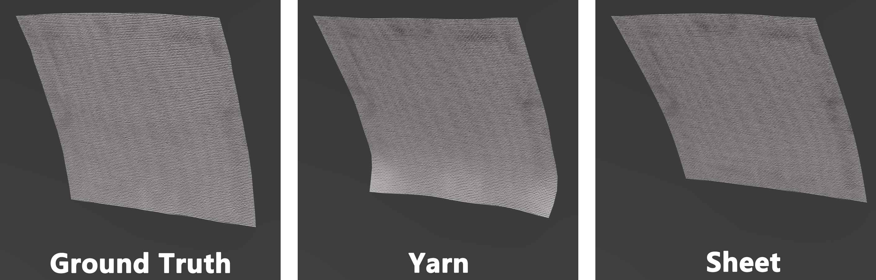
Figure 10: The visual learning results of the differentiable sheet-level simulator (Liang et al., 2019) and our model learns on the data generate by (Narain et al., 2012)

Parameters. We induce prior knowledge to limit the parameter learning within valid ranges, so that the multi-solution problem, also met by existing methods, can be mitigated. All cloths we used are made of two types of yarns. We use the same range, $d\in[0.001,0.003]$, $b\in[0.00005,0.00018]$, $S\in[0,1200]$ and $\mu\in[0,1.0]$ for both yarns, where $d$, $b$, $S$ and $\mu$ are the density, bending modulus, shear modulus and friction coefficient respectively. We use $s_{1}\in[0,800000]$ and $s_{2}\in[0,300000]$ for the stretching for both yarns. For other coefficients, we use $k_{f}=1000$ and $d_{f}=1000$ in the friction force, $c=3$ and $\sigma=0.6$ in the shear force, $k_{c}=1$ in yarn-to-yarn collision in all experiments.

When training our model on the data generated by a sheet-level cloth simulator (Narain et al., 2012), we use a pure woven cloth made of one type of yarn. This is because it is not possible to specify multiple yarn behaviors in a sheet simulator, so we use a pure yarn cloth for generating the ground truth. The cloth parameters are from the ‘white-dots-on-black’ cloth in Wang et al. (2011) which is 100 percent polyester. To learn from it, we employ all three woven patterns in our model as there is no prior knowledge about the woven pattern of the ‘white-dots-on-black’ cloth. We also fix the friction coefficient $\mu=0.5$ and impose the ranges on parameters shown in Table 9. Finally, we would like to point it out in real-world applications, information such as woven patterns and yarn materials are easily available so that the ranges of parameter values such as density, bending and stretching can be obtained. Although the knowledge of shearing and friction cannot be easily acquired, the ranges we use are general enough.

Table 5: Testing errors ($\times 10^{-6}$) of our model and (Liang et al., 2019) trained on 5, 10 and 25 frames generated by (Narain et al., 2012).

fabrics/frames	5	10	25
Plain-(1,2)	$6.702$	$1.167$	$0.496$
Satin-(1,2)	$7.972$	$1.225$	$0.624$
Twill-(1,2)	$8.218$	$1.772$	$0.776$
(Liang et al., 2019)	$4.098$	$4.752$	$1.716$

Note that in all experiments, the prior knowledge we induce is only a weak prior, i.e. using the same general ranges for multiple experiments across different woven patterns, so that the learning success still lies in our model’s ability to infer the right parameter values.

Parameter Initialization.

The material estimation results are affected by initialization. To test if our model can learn stably, we report the mean and the standard deviation of multiple experiments with different parameter initial values. The initial values of the physical parameters are randomly selected from a range of $\pm 10\%$ of the average of the two yarns. For instance, in learning the stretch in Plain-(1,2), we only know the ranges of the stretching parameters Y1 and Y2 of Yarn1 and Yarn2 but not the exact values. Therefore, when initializing Y1 and Y2, we randomly sample values from a range of $\pm 10\%$ of the mean stretch stiffness of the Yarn1 and Yarn2, $[\mbox{mean(Y1, Y2)}\times 0.9,\mbox{mean(Y1, Y2)}\times 1.1]$ for initialization. The results of the 5 repetitions are shown Table 6 and Table 7. Given that the standard deviations are small, it shows that our model can stably learn reasonable parameter values.

Different Force Magnitude.

To evaluate the influence of the wind force, we conduct experiments using 5N, 10N, and 15N wind force to blow a piece of $17\times 17$ Plain-(1,2) cloth. The learning result is shown in the Table 8 which demonstrate wind force strength has ignorable influence on the learned parameters.

Table 6: Learning cloth parameters with different initial values (part one).

Size	Shear $S$	Friction $\mu$
$5\times 5$	$1011.79\pm 6.12$	$0.39\pm 0.08$
$10\times 10$	$983.41\pm 6.84$	$0.44\pm 0.03$
$17\times 17$	$962.29\pm 8.99$	$0.47\pm 0.06$

Table 7: Learning cloth parameters with different initial values (part two).

Size	Yarn	Density	Stretch	Bend
$5\times 5$	1	$1.98\text{\times}{10}^{-3}$$\pm$$3.00\text{\times}{10}^{-5}$	$498595\pm 8862$	$1.37\text{\times}{10}^{-4}$$\pm$$1.41\text{\times}{10}^{-6}$
	2	$2.45\text{\times}{10}^{-3}$$\pm$$4.81\text{\times}{10}^{-5}$	$186710\pm 3776$	$1.11\text{\times}{10}^{-4}$$\pm$$4.78\text{\times}{10}^{-6}$
$10\times 10$	1	$2.03\text{\times}{10}^{-3}$$\pm$$5.04\text{\times}{10}^{-5}$	$542375\pm 7099$	$1.44\text{\times}{10}^{-4}$$\pm$$2.08\text{\times}{10}^{-6}$
	2	$2.47\text{\times}{10}^{-3}$$\pm$$4.73\text{\times}{10}^{-5}$	$180032\pm 1848$	$1.05\text{\times}{10}^{-4}$$\pm$$8.18\text{\times}{10}^{-6}$
$17\times 17$	1	$2.00\text{\times}{10}^{-3}$$\pm$$6.66\text{\times}{10}^{-5}$	$519993\pm 3175$	$1.43\text{\times}{10}^{-4}$$\pm$$5.55\text{\times}{10}^{-6}$
	2	$2.45\text{\times}{10}^{-3}$$\pm$$5.04\text{\times}{10}^{-5}$	$176232\pm 1514$	$1.19\text{\times}{10}^{-4}$$\pm$$6.50\text{\times}{10}^{-6}$

Table 8: Learning cloth physical parameters with different wind force.

Wind	Shear $S$	Friction $\mu$	Yarn	Density	Stretch	Bend
5	$947$	0.402	1	$1.969\text{\times}{10}^{-3}$	505421	$1.323\text{\times}{10}^{-4}$
			2	$2.440\text{\times}{10}^{-3}$	171304	$1.034\text{\times}{10}^{-4}$
10	$942$	0.520	1	$2.026\text{\times}{10}^{-3}$	494109	$1.311\text{\times}{10}^{-4}$
			2	$2.441\text{\times}{10}^{-3}$	168267	$1.049\text{\times}{10}^{-4}$
15	934	0.586	1	$2.029\text{\times}{10}^{-3}$	487918	$1.341\text{\times}{10}^{-4}$
			2	$2.437\text{\times}{10}^{-3}$	167601	$1.066\text{\times}{10}^{-4}$

Influence of Woven Patterns.

The investigation on different woven patterns is crucial as they affect the cloth dynamics significantly. To show this, we conducted simulations of three pieces of cloths with the same parameters, but with different woven patterns. We shear three pieces of cloth then release them. The Figure 11 shows three pieces of cloth in the initial state and 10 steps later. There are obvious differences after merely 10 steps. This demonstrates woven patterns have considerable influences on the overall mechanical properties.

Figure 11: Three pieces of cloth woven in different patterns show different dynamics.

Table 9: Cloth parameters’ initial values and ranges when ground-truth generated by sheet-level cloth simulator(Narain et al., 2012)

Name	Density($kg/m$)	Stretch($N/m$)	Bend($N/m$)	Shear($N/m$)
Value	0.004	1e6	0.0001	20000
Upper limit	0.008	2e6	0.0002	30000
Lower limit	0.001	0	0	0

Table 10: Testing errors ($\times 10^{-6}$) of our model (left) and (Liang et al., 2019) (right) trained on 5, 10 and 25 frames. Ground-truth generated by a yarn-level simulator (Cirio et al., 2014).

fabrics/frames	5	10	25	5	10	25
Plain-(1,2)	$1.152\text{\times}{10}^{-4}$	$1.068\text{\times}{10}^{-4}$	$3.962\text{\times}{10}^{-5}$	$1.462$	0.7375	0.4124
Plain-(1,3)	$1.516\text{\times}{10}^{-4}$	$1.268\text{\times}{10}^{-4}$	$3.555\text{\times}{10}^{-5}$	$1.608$	0.7906	0.4567
Plain-(2,3)	$5.233\text{\times}{10}^{-4}$	$1.291\text{\times}{10}^{-4}$	$2.117\text{\times}{10}^{-5}$	$1.952$	0.5999	0.2294
Satin-(1,2)	$1.134\text{\times}{10}^{-4}$	$1.070\text{\times}{10}^{-4}$	$4.285\text{\times}{10}^{-5}$	$1.466$	0.7405	0.4146
Satin-(1,3)	$1.551\text{\times}{10}^{-4}$	$1.355\text{\times}{10}^{-4}$	$4.362\text{\times}{10}^{-5}$	$1.624$	0.8004	0.4445
Satin-(2,3)	$6.254\text{\times}{10}^{-4}$	$1.355\text{\times}{10}^{-4}$	$4.413\text{\times}{10}^{-5}$	$2.128$	0.5949	0.2265
Twill-(1,2)	$1.130\text{\times}{10}^{-4}$	$1.068\text{\times}{10}^{-4}$	$4.208\text{\times}{10}^{-5}$	$1.472$	0.7451	0.4160
Twill-(1,3)	$1.550\text{\times}{10}^{-4}$	$1.349\text{\times}{10}^{-4}$	$4.200\text{\times}{10}^{-5}$	$1.633$	0.8059	0.4577
Twill-(2,3)	$6.470\text{\times}{10}^{-4}$	$1.352\text{\times}{10}^{-4}$	$4.938\text{\times}{10}^{-5}$	$2.181$	0.5994	0.2278

A.2 Visual results

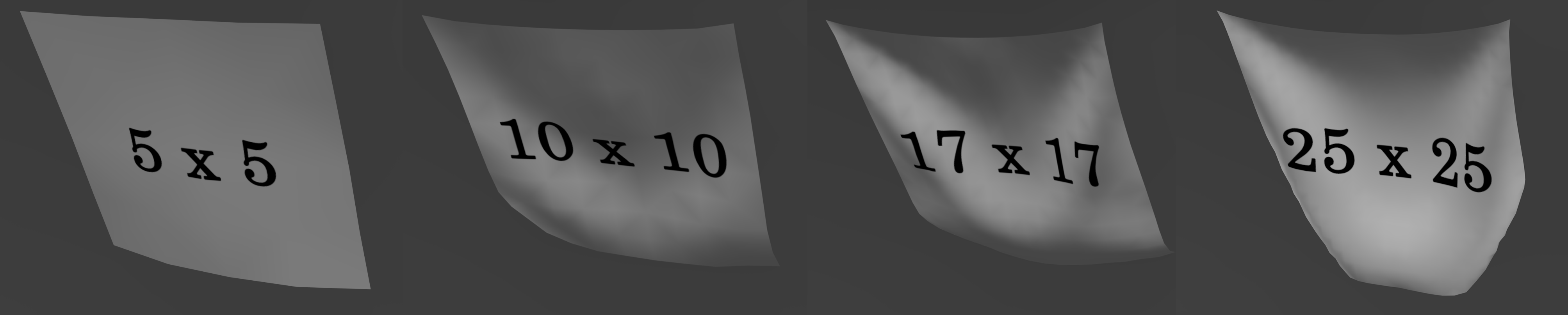
Figure 12: The visual results of our model learning on different cloth sizes. From left to right: $5\times 5$, $10\times 10$, $17\times 17$ and $25\times 25$.

Here we show some snapshots of our model on cloths of different sizes in Figure 12. As expected, small cloths tend to show low dynamics and appear to be more ‘rigid’. Bigger cloths tend to have more subtle dynamics such as wrinkles, even under the same external impact, i.e. gravity and wind with a constant magnitude. More visual results can be found in the supplementary video.

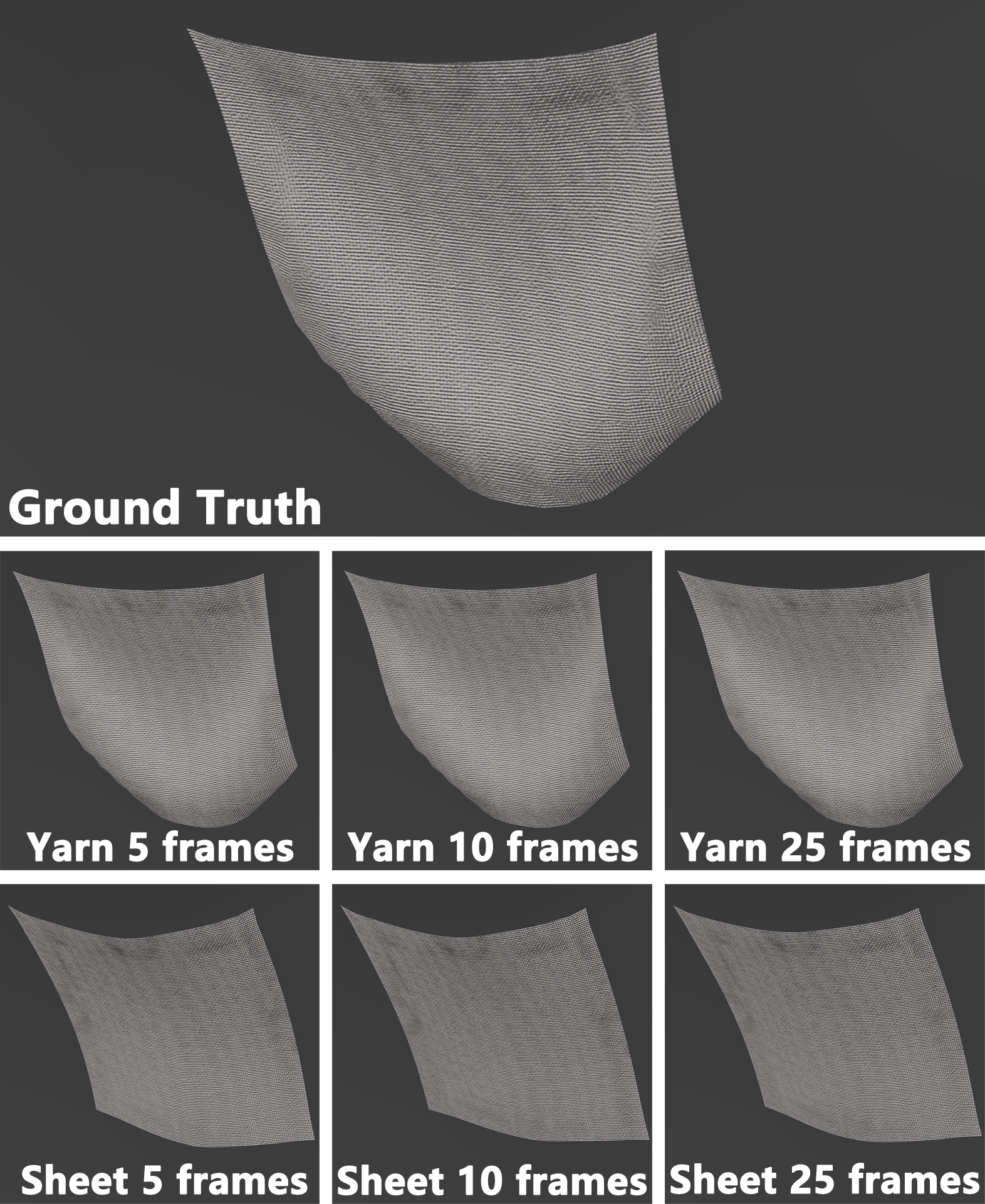
Figure 13: The visual results of Plain-(1, 2) ground-truth, our model, and sheet-level model trained with different number of frames. The snapshots are the 133$th$ frame of the simulations after learning.

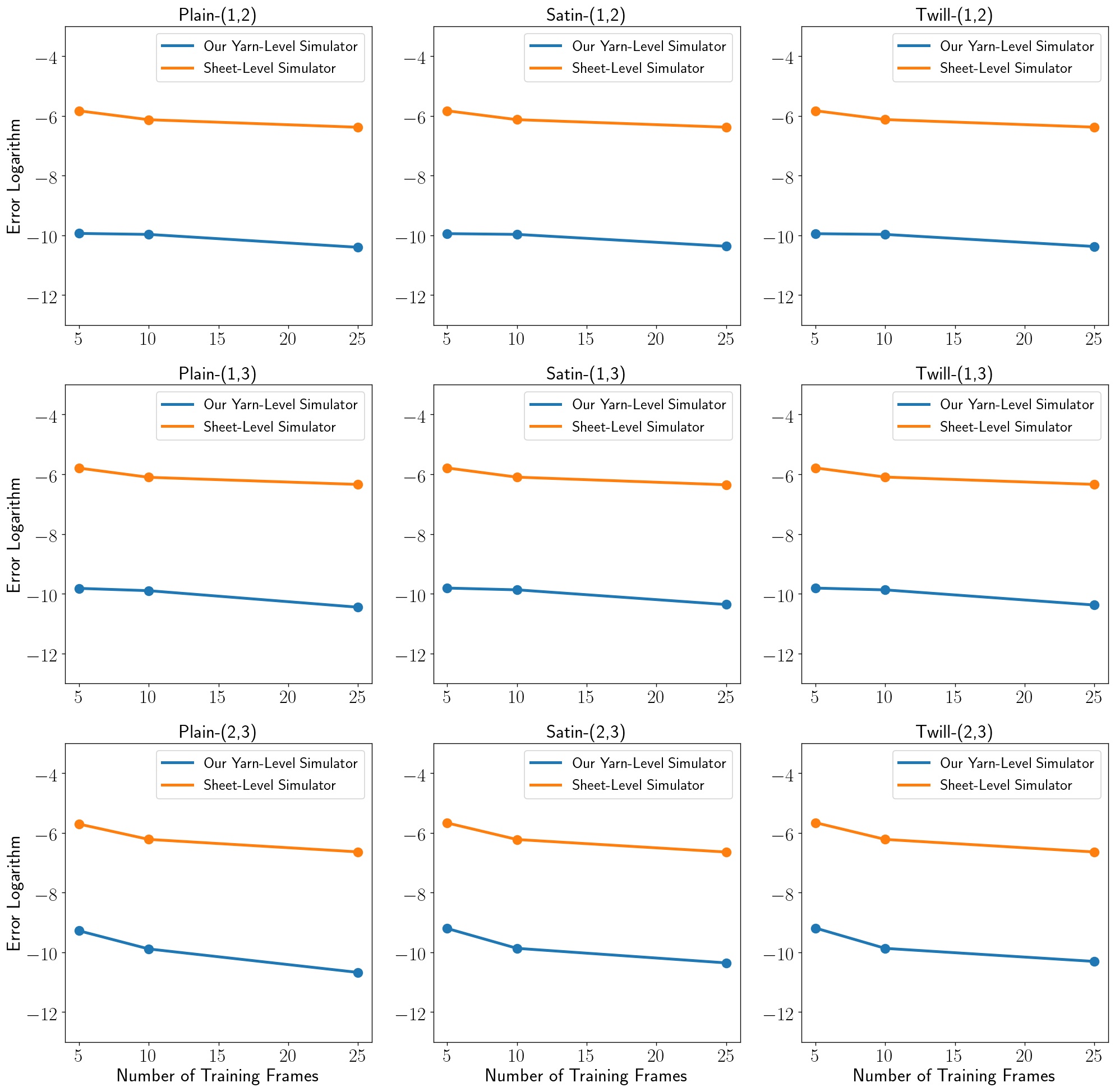
Figure 14: Prediction error logarithm vs training data.

Table 11: Learned parameters by Bayesian Optimization on different kinds of fabrics.

Frames	Density	Stretch	Bend	Density	Stretch	Bend
5	$2.483\text{\times}{10}^{-3}$	647270	$0.636\text{\times}{10}^{-4}$	$2.125\text{\times}{10}^{-3}$	270641	$1.576\text{\times}{10}^{-4}$
10	$2.176\text{\times}{10}^{-3}$	577235	$0.798\text{\times}{10}^{-4}$	$2.264\text{\times}{10}^{-3}$	217144	$1.542\text{\times}{10}^{-4}$
25	$2.328\text{\times}{10}^{-3}$	537434	$1.687\text{\times}{10}^{-4}$	$2.097\text{\times}{10}^{-3}$	249896	$0.976\text{\times}{10}^{-4}$
5	$2.202\text{\times}{10}^{-3}$	605289	$1.403\text{\times}{10}^{-4}$	$2.349\text{\times}{10}^{-3}$	272153	$0.868\text{\times}{10}^{-4}$
10	$1.669\text{\times}{10}^{-3}$	257877	$1.582\text{\times}{10}^{-4}$	$2.635\text{\times}{10}^{-3}$	268451	$0.529\text{\times}{10}^{-4}$
25	$1.454\text{\times}{10}^{-3}$	315715	$1.213\text{\times}{10}^{-4}$	$2.950\text{\times}{10}^{-3}$	23702	$1.656\text{\times}{10}^{-4}$
5	$2.514\text{\times}{10}^{-3}$	250093	$1.611\text{\times}{10}^{-4}$	$2.363\text{\times}{10}^{-3}$	20371	$0.985\text{\times}{10}^{-4}$
10	$2.964\text{\times}{10}^{-3}$	164021	$0.524\text{\times}{10}^{-4}$	$2.255\text{\times}{10}^{-3}$	49648	$1.225\text{\times}{10}^{-4}$
25	$2.414\text{\times}{10}^{-3}$	73734	$0.890\text{\times}{10}^{-4}$	$2.436\text{\times}{10}^{-3}$	267452	$1.113\text{\times}{10}^{-4}$

A.3 Yarn-level versus Sheet-level

A full comparison between our model and (Liang et al., 2019) is shown in Table 10, where a yarn-level simulator (Cirio et al., 2016) is used to generate the ground-truth. We exhaustively conduct comparisons using all combinations of yarns and woven patterns. We can see that our model is consistently better than (Liang et al., 2019) by large margins. Visually, we show snapshots in Figure 13. The sheet model results are in general more rigid and do not contain as much subtle dynamics as ours do, across different training frame numbers. Since 5, 10 and 25 frames contain different amounts of information on (subtle) motion dynamics, Figure 13 shows that there is a lack of granularity in the sheet model when capturing subtle dynamics compared with ours.

Further, we also show the plots on the data efficiency in Figure 14, under all 9 yarn-woven pattern combinations, across different amounts of training data. In all settings, our data efficiency is significantly higher. By extrapolation, it would take a large number of extra training frames for the sheet-level model to achieve similar accuracy. More comparisons are also available in the supplementary video.

A.4 Our model versus Bayesian Optimization

Table 12 shows the testing errors of the Bayesian Optimization. Although the MSE errors are small, the learned parameters are far from the ground truth (shown in the Table 11), which is somewhat surprising. After examining the results, we find that Bayesian Optimization suffers from the multi-solution problem so that it merely gives a set of working parameters instead of the true parameters. In other words, although the prediction error is low, physically speaking, the learned parameters are far from the true materials. This happens even when we use the same parameter ranges as in our model. This is an intrinsic property of Bayesian optimization which is based on sampling, and therefore difficult to avoid during learning.

Table 12: Testing error ($\times 10^{-6}$) of Bayesian Optimization with yarn-level simulator (Cirio et al., 2016) learned on 5, 10, and 25 frames.

Fabrics/Frames	5	10	25
Plain-(1,2)	$0.512$	$0.176$	$0.109$
Plain-(1,3)	$1.280$	$1.269$	$0.738$
Plain-(2,3)	$28.19$	$19.22$	$18.16$

A.5 Control Experiment Setting

The control experiment scenario is illustrated in the Figure 15.

Figure 15: A square cloth is thrown from the table into the black box by four forces applied on the four corners of the cloth.

A.6 Significant Error in Visual

We discussed the significance of the small error in physics-based simulation. Figure 16 and Figure 17 visually prove our explanations in the main paper: the error accumulates over time and increases with increasing cloth size.

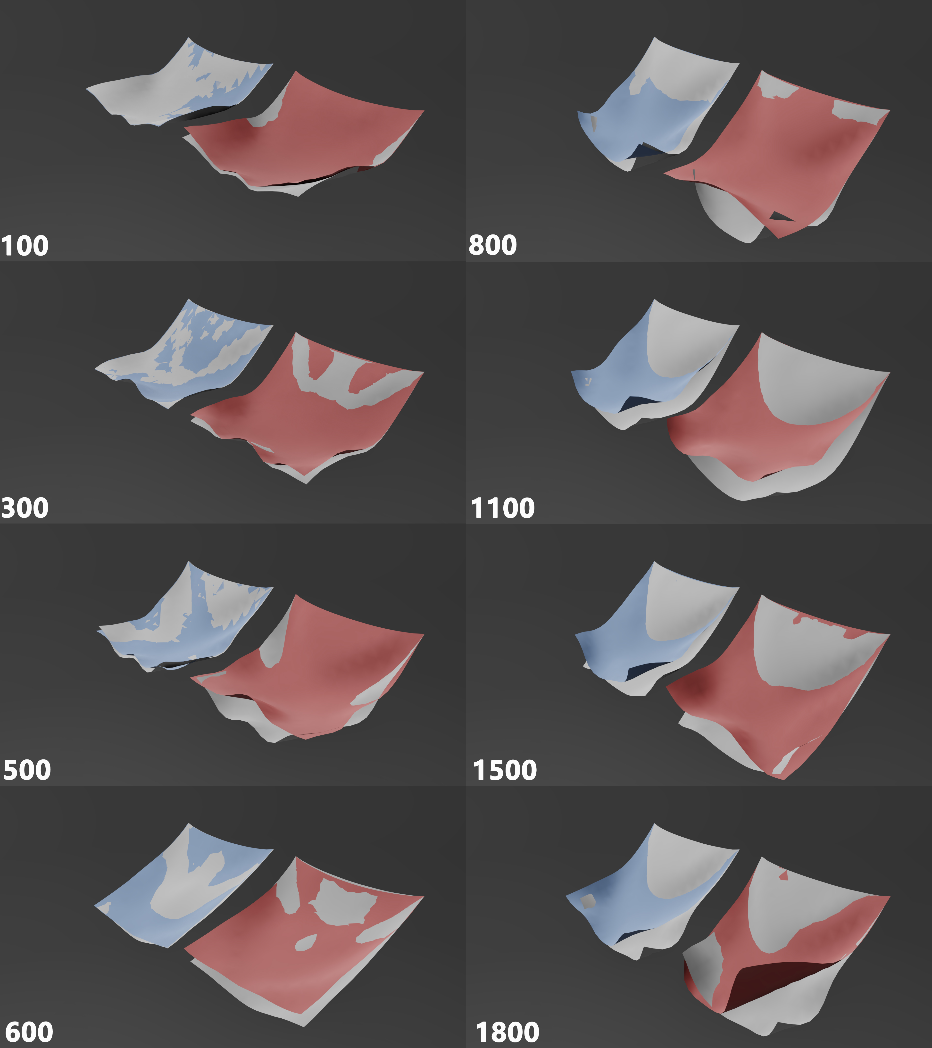
Figure 16: Visual differences in long simulations. The grey cloth is ground truth. The blue cloth and the red cloth are simulated with the parameters learned by our model and BO. The blue cloth shows smaller visual differences than the red one.

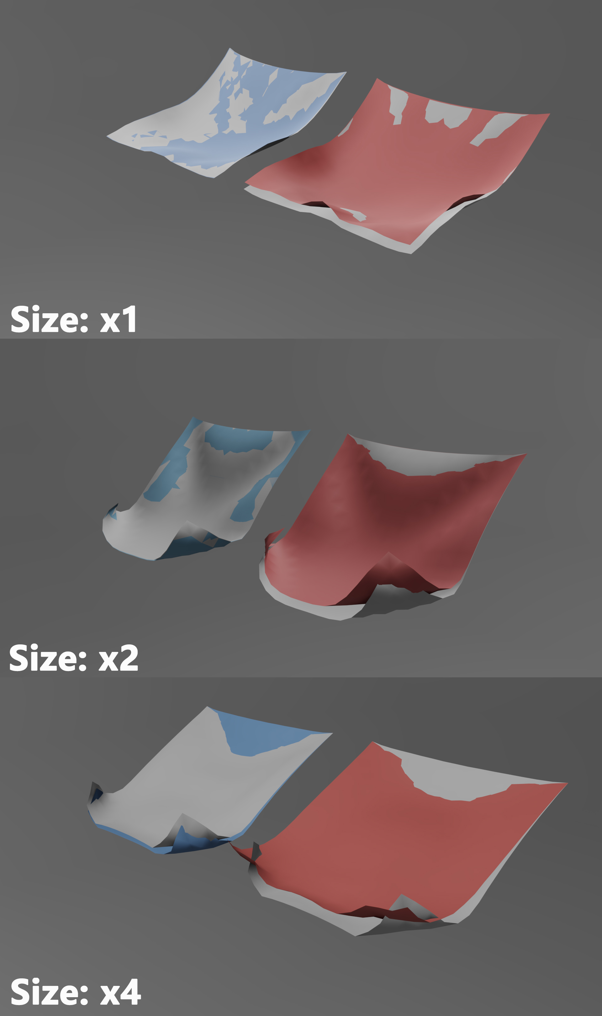
Figure 17: Visual differences on larger cloths and long simulation (500 steps). The grey cloth is ground truth. The blue cloth and the red cloth are simulated with the parameters learned by our model and BO. The blue cloth shows smaller differences than the red one.

Appendix B Differentiable Yarn-level Cloth Simulator

In this section, we give the full details of our model and mathematical derivation.

B.1 Intro yarn force models

Figure 18: Blue and red rods denote warps and wefts respectively. $\mathbf{q}$s are the crossing nodes.

Representing the cloth as in Figure 18, we employ an EoL discretization (Sueda et al., 2011) and denote the spatial positions of crossing nodes in Lagrangian coordinates and represent the contact sliding movement in Eulerian coordinates, $\mathbf{q}_{i}\equiv(\mathbf{x}_{i},u_{i},v_{i})$ where $\mathbf{x}_{i}\in\mathbb{R}^{3}$ implies crossing node $i$’s spatial position and $(u_{i},v_{i})$ the node’s position in the material frame. The two end points of yarns are taken as special crossing nodes as they do not contact with other yarns and therefore have no Eulerian terms, i.e. $\mathbf{q}_{j}\equiv\mathbf{x}_{i}$. Therefore, on a $r(rows)\times c(columns)$ cloth, there are $(r-2)\times(c-2)$ crossing nodes with five Degrees of Freedom (DoFs) and $2r+2c-4$ crossing nodes with three DoFs. Every two neighboring crossing nodes on the same warp/weft delimit a warp/weft segment. A warp segment whose two end points are $\mathbf{q}_{0}$ and $\mathbf{q}_{1}$ is denoted as $\mathbf{[q_{0},q_{1}]}$ and its position is $(\mathbf{x}_{0},\mathbf{x}_{1},u_{0},u_{1})$ (shown in 18). This way, a woven cloth is discretized into crossing nodes and segments which are the primitive units of the simulated cloth. Every segment is assumed to be straight so that linear interpolation can be employed on the segment, e.g. the spatial position of a point in the segment $\mathbf{[q_{0},q_{1}]}$ is $\mathbf{x}(u)=\frac{u-u_{0}}{\Delta u}\mathbf{x}_{0}+\frac{u_{1}-u}{\Delta u}\mathbf{x}_{1}$, where $u$ is the point’s position in Eulerian coordinates and $\Delta u=u_{1}-u_{0}$ is the length of the segment. We use $L$ to denote the distances between neighbor yarns and $R$ to denote the yarn radius.

B.2 System Equation for Simulation

A cloth’s state at time $t$, $\mathcal{S}_{(t)}=\{\mathcal{Q}_{(t)},\dot{\mathcal{Q}}_{(t)}\}$, includes all its crossing nodes’ positions $\mathcal{Q}=\{\mathbf{q}_{i}|i=1,2,\dots,N\}$ and velocities $\dot{\mathcal{Q}}=\{\dot{\mathbf{q}}_{i}|i=1,2,\dots,N\}$, where $N$ is the number of crossing nodes. Knowing the states, then we can calculate the internal and external forces:

$$\mathbf{F}=\mathbf{M}\ddot{\mathbf{q}}=\frac{\partial T}{\partial\mathbf{q}}-\frac{\partial V}{\partial\mathbf{q}}-\dot{\mathbf{M}}\dot{\mathbf{q}}$$ (6)

where $\mathbf{q}$, $\dot{\mathbf{q}}$, and $\ddot{\mathbf{q}}$ are the nodes general position, velocity, and acceleration respectively, with a dimension $l=3\times r\times c+2\times(r-2)\times(c-2)$. $\mathbf{M}\in\mathbb{R}^{l\times l}$ is the general mass matrix. The model assumes mass is distributed homogeneously in one segment, so the mass matrix of a warp segment $[\mathbf{q}_{0},\mathbf{q}_{1}]$ is

$$\mathbf{M}_{0,1}=\frac{1}{6}\Delta u\rho\begin{pmatrix}2\mathbf{I}_{3}&\mathbf{I}_{3}&-2\mathbf{w}&-\mathbf{w}\\ \mathbf{I}_{3}&2\mathbf{I}_{3}&-\mathbf{w}&-2\mathbf{w}\\ -2\mathbf{w}^{\top}&-\mathbf{w}^{\top}&2\mathbf{w}^{\top}\mathbf{w}&\mathbf{w}^{\top}\mathbf{w}\\ -\mathbf{w}^{\top}&-2\mathbf{w}^{\top}&\mathbf{w}^{\top}\mathbf{w}&2\mathbf{w^{\top}w}\\ \end{pmatrix}$$ (7)

where $\mathbf{w}=\frac{\mathbf{x}_{1}-\mathbf{x}_{0}}{\Delta u}$, and $\rho$ is yarn density. $T$ and $V$ are the kinetic and potential energy respectively. As the partial derivative of energy with respect to position is force, the right hand terms in Equation 6 are inertia, conservative forces, and part of the time derivative of $\mathbf{M}\dot{\mathbf{q}}$. Non-conservative forces are added to the right side of the equation.

We employ implicit Euler for stability in large steps (Baraff & Witkin, 1998). Given the acceleration $\ddot{\mathbf{q}}=\mathbf{M}^{-1}\mathbf{F}$ and the change of speed over time step $h$, $\Delta\dot{\mathbf{q}}$ can be approximated by $\Delta\dot{\mathbf{q}}=h\mathbf{M}^{-1}\mathbf{F}_{(t+1)}$, where $\mathbf{F}_{(t+1)}$ is the force at $t+1$ that can be approximated by first-order Taylor expansion $\mathbf{F}_{(t+1)}=\mathbf{F}_{(t)}+\frac{\partial\mathbf{F}_{(t)}}{\partial\mathbf{q}}\Delta\mathbf{q}+\frac{\partial\mathbf{F}_{(t)}}{\partial\dot{\mathbf{q}}}\Delta\dot{\mathbf{q}}$, where $\mathbf{F}_{(t)}$ is the force at $t$ which can be computed by Equation 6. Then node positions at $t+1$ are $\mathbf{q}_{(t+1)}=\mathbf{q}_{(t)}+h(\dot{\mathbf{q}}_{(t)}+\Delta\dot{\mathbf{q}})$. Finally, we have the system equation for simulation:

$$\left(\mathbf{M}-\frac{\partial\mathbf{F}_{(t)}}{\partial\mathbf{q}}h^{2}-\frac{\partial\mathbf{F}_{(t)}}{\partial\dot{\mathbf{q}}}h\right)\dot{\mathbf{q}}_{(t+1)}=h\left(\mathbf{F}_{(t)}-\frac{\partial\mathbf{F}_{(t)}}{\partial\dot{\mathbf{q}}}\right)+\mathbf{M}\dot{\mathbf{q}}_{(t)}$$ (8)

To solve Equation 8, we explain every term including the general mass matrix $\mathbf{M}$ and every force contained in $\mathbf{F}_{(t)}$ below.

B.3 General Mass Matrix

The mass matrix of a warp segment $[\mathbf{q}_{0},\mathbf{q}_{1}]$ is

$$\mathbf{M}_{0,1}=\frac{1}{6}\Delta u\rho\begin{pmatrix}2\mathbf{I}_{3}&\mathbf{I}_{3}&-2\mathbf{w}&-\mathbf{w}\\ \mathbf{I}_{3}&2\mathbf{I}_{3}&-\mathbf{w}&-2\mathbf{w}\\ -2\mathbf{w}^{\top}&-\mathbf{w}^{\top}&2\mathbf{w}^{\top}\mathbf{w}&\mathbf{w}^{\top}\mathbf{w}\\ -\mathbf{w}^{\top}&-2\mathbf{w}^{\top}&\mathbf{w}^{\top}\mathbf{w}&2\mathbf{w^{\top}w}\\ \end{pmatrix}$$ (9)

where $\Delta u=u_{1}-u_{0}$ is the distance between the two nodes in Eulerian coordinates, $\mathbf{w}=\frac{\mathbf{x}_{1}-\mathbf{x}_{0}}{\Delta u}$, and $\rho$ is yarn’s linear density. The partial derivatives of general mass matrix with respect to nodes’ position is

$$\begin{pmatrix}\frac{\partial\mathbf{M}_{0,1}}{\partial\mathbf{x}_{0}}&\frac{\partial\mathbf{M}_{0,1}}{\partial\mathbf{x}_{1}}&\frac{\partial\mathbf{M}_{0,1}}{\partial u_{0}}&\frac{\partial\mathbf{M}_{0,1}}{\partial u_{1}}\end{pmatrix}^{\top}$$ (10)

As $\mathbf{x}_{0}$ and $\mathbf{x}_{1}$ are vectors:

$$\frac{\partial\mathbf{M}_{0,1}}{\partial\mathbf{x}_{0}}=\begin{pmatrix}\frac{\partial\mathbf{M}_{0,1}}{\partial\mathbf{x}_{0}^{(1)}}\\ \frac{\partial\mathbf{M}_{0,1}}{\partial\mathbf{x}_{0}^{(2)}}\\ \frac{\partial\mathbf{M}_{0,1}}{\partial\mathbf{x}_{0}^{(3)}}\end{pmatrix}\mbox{and}\;\frac{\partial\mathbf{M}_{0,1}}{\partial\mathbf{x}_{1}}=\begin{pmatrix}\frac{\partial\mathbf{M}_{0,1}}{\partial\mathbf{x}_{1}^{(1)}}\\ \frac{\partial\mathbf{M}_{0,1}}{\partial\mathbf{x}_{1}^{(2)}}\\ \frac{\partial\mathbf{M}_{0,1}}{\partial\mathbf{x}_{1}^{(3)}}\end{pmatrix}$$ (11)

The component $\frac{\partial\mathbf{M}_{0,1}}{\partial\mathbf{x}_{0}^{(1)}}$ is

$$\frac{\partial\mathbf{M}_{0,1}}{\partial\mathbf{x}_{0}^{(1)}}=\frac{1}{6}\Delta u\rho\begin{pmatrix}\mathbf{0}&\mathbf{0}&-2\frac{\partial\mathbf{w}}{\partial\mathbf{x}_{0}^{(1)}}&-\frac{\partial\mathbf{w}}{\partial\mathbf{x}_{0}^{(1)}}\\ \mathbf{0}&\mathbf{0}&-\frac{\partial\mathbf{w}}{\partial\mathbf{x}_{0}^{(1)}}&-2\frac{\partial\mathbf{w}}{\partial\mathbf{x}_{0}^{(1)}}\\ -2\frac{\partial\mathbf{w}^{\top}}{\partial\mathbf{x}_{0}^{(1)}}&-\frac{\partial\mathbf{w}^{\top}}{\partial\mathbf{x}_{0}^{(1)}}&2\frac{\partial\mathbf{w}^{\top}\mathbf{w}}{\partial\mathbf{x}_{0}^{(1)}}&\frac{\partial\mathbf{w}^{\top}\mathbf{w}}{\partial\mathbf{x}_{0}^{(1)}}\\ -\frac{\partial\mathbf{w}^{\top}}{\partial\mathbf{x}_{0}^{(1)}}&-2\frac{\partial\mathbf{w}^{\top}}{\partial\mathbf{x}_{0}^{(1)}}&\frac{\partial\mathbf{w}^{\top}\mathbf{w}}{\partial\mathbf{x}_{0}^{(1)}}&2\frac{\partial\mathbf{w}^{\top}\mathbf{w}}{\partial\mathbf{x}_{0}^{(1)}}\end{pmatrix}$$

and $\frac{\partial\mathbf{M}_{0,1}}{\partial\mathbf{x}_{0}^{(2)}}$, $\frac{\partial\mathbf{M}_{0,1}}{\partial\mathbf{x}_{0}^{(3)}}$, $\frac{\partial\mathbf{M}_{0,1}}{\partial\mathbf{x}_{1}^{(1)}}$, $\frac{\partial\mathbf{M}_{0,1}}{\partial\mathbf{x}_{1}^{(2)}}$ and $\frac{\partial\mathbf{M}_{0,1}}{\partial\mathbf{x}_{1}^{(3)}}$ are in a similar form as $\frac{\partial\mathbf{M}_{0,1}}{\partial\mathbf{x}_{0}^{(1)}}$. In each term, we have:

$$\frac{\partial\mathbf{w}}{\partial\mathbf{x}_{0}^{(1)}}=-\begin{pmatrix}\frac{1}{\Delta u}\\ 0\\ 0\end{pmatrix}\mbox{,}\;\frac{\partial\mathbf{w}}{\partial\mathbf{x}_{0}^{(2)}}=-\begin{pmatrix}0\\ \frac{1}{\Delta u}\\ 0\end{pmatrix}\mbox{, and}\;\frac{\partial\mathbf{w}}{\partial\mathbf{x}_{0}^{(3)}}=-\begin{pmatrix}0\\ 0\\ \frac{1}{\Delta u}\end{pmatrix}$$

$$\frac{\partial\mathbf{w}}{\partial\mathbf{x}_{1}^{(1)}}=\begin{pmatrix}\frac{1}{\Delta u}\\ 0\\ 0\end{pmatrix}\mbox{,}\;\frac{\partial\mathbf{w}}{\partial\mathbf{x}_{1}^{(2)}}=\begin{pmatrix}0\\ \frac{1}{\Delta u}\\ 0\end{pmatrix}\mbox{, and}\;\frac{\partial\mathbf{w}}{\partial\mathbf{x}_{1}^{(3)}}=\begin{pmatrix}0\\ 0\\ \frac{1}{\Delta u}\end{pmatrix}$$

$$\frac{\partial\mathbf{w}^{\top}\mathbf{w}}{\partial\mathbf{x}_{0}^{(1)}}=\frac{\partial\mathbf{w}^{\top}}{\partial\mathbf{x}_{0}^{(1)}}\mathbf{w}+\mathbf{w}^{\top}\frac{\partial\mathbf{w}}{\partial\mathbf{x}_{0}^{(1)}}=-2\frac{\mathbf{x}_{1}^{(1)}-\mathbf{x}_{0}^{(1)}}{\Delta u^{2}}$$

where $\frac{\partial\mathbf{w}^{\top}\mathbf{w}}{\partial\mathbf{x}_{0}^{(2)}}$, $\frac{\partial\mathbf{w}^{\top}\mathbf{w}}{\partial\mathbf{x}_{0}^{(3)}}$, $\frac{\partial\mathbf{w}^{\top}\mathbf{w}}{\partial\mathbf{x}_{1}^{(1)}}$, $\frac{\partial\mathbf{w}^{\top}\mathbf{w}}{\partial\mathbf{x}_{1}^{(2)}}$ and $\frac{\partial\mathbf{w}^{\top}\mathbf{w}}{\partial\mathbf{x}_{1}^{(3)}}$ have a similar form as $\frac{\partial\mathbf{w}^{\top}\mathbf{w}}{\partial\mathbf{x}_{0}^{(1)}}$.

Unsurprisingly, we can find that

$$\frac{\partial\mathbf{M}_{0,1}}{\partial\mathbf{x}_{0}^{(1)}}=-\frac{\partial\mathbf{M}_{0,1}}{\partial\mathbf{x}_{1}^{(1)}}\;\mbox{,}\;\frac{\partial\mathbf{M}_{0,1}}{\partial\mathbf{x}_{0}^{(2)}}=-\frac{\partial\mathbf{M}_{0,1}}{\partial\mathbf{x}_{1}^{(2)}}\;\mbox{and}\;\frac{\partial\mathbf{M}_{0,1}}{\partial\mathbf{x}_{0}^{(3)}}=-\frac{\partial\mathbf{M}_{0,1}}{\partial\mathbf{x}_{1}^{(3)}}$$

After deriving the partial derivatives of $\mathbf{M}_{0,1}$ with respect to the Lagrangian coordinates, we give its partial derivatives with respect to Eulerian coordinates:

$$\frac{\partial\mathbf{M}_{0,1}}{\partial u_{0}}= -\frac{1}{6}\rho\begin{pmatrix}2\mathbf{I}_{3}&\mathbf{I}_{3}&-2\mathbf{w}&-\mathbf{w}\\ \mathbf{I}_{3}&2\mathbf{I}_{3}&-\mathbf{w}&-2\mathbf{w}\\ -2\mathbf{w}^{\top}&-\mathbf{w}^{\top}&2\mathbf{w}^{\top}\mathbf{w}&\mathbf{w}^{\top}\mathbf{w}\\ -\mathbf{w}^{\top}&-2\mathbf{w}^{\top}&\mathbf{w}^{\top}\mathbf{w}&2\mathbf{w^{\top}w}\\ \end{pmatrix}$$

$$+\frac{1}{6}\Delta u\rho\begin{pmatrix}\mathbf{0}&\mathbf{0}&-2\frac{\partial\mathbf{w}}{\partial u_{0}}&-\frac{\partial\mathbf{w}}{\partial u_{0}}\\ \mathbf{0}&\mathbf{0}&-\frac{\partial\mathbf{w}}{\partial u_{0}}&-2\frac{\partial\mathbf{w}}{\partial u_{0}}\\ -2\frac{\partial\mathbf{w}^{\top}}{\partial u_{0}}&-\frac{\partial\mathbf{w}^{\top}}{\partial u_{0}}&2\frac{\partial\mathbf{w}^{\top}\mathbf{w}}{\partial u_{0}}&\frac{\partial\mathbf{w}^{\top}\mathbf{w}}{\partial u_{0}}\\ -\frac{\partial\mathbf{w}^{\top}}{\partial u_{0}}&-2\frac{\partial\mathbf{w}^{\top}}{\partial u_{0}}&\frac{\partial\mathbf{w}^{\top}\mathbf{w}}{\partial u_{0}}&2\frac{\partial\mathbf{w}^{\top}\mathbf{w}}{\partial u_{0}}\end{pmatrix}$$ (12)

where $\frac{\partial\mathbf{M}_{0,1}}{\partial u_{1}}$ has a similar form as $\frac{\partial\mathbf{M}_{0,1}}{\partial u_{0}}$ and:

$$\frac{\partial\mathbf{w}}{\partial u_{0}}=\frac{\mathbf{x}_{1}-\mathbf{x}_{0}}{\Delta u^{2}}=\frac{\mathbf{w}}{\Delta u}\;\mbox{and}\;\frac{\partial\mathbf{w}}{\partial u_{1}}=-\frac{\mathbf{x}_{1}-\mathbf{x}_{0}}{\Delta u^{2}}=-\frac{\mathbf{w}}{\Delta u}$$

$$\frac{\partial\mathbf{w}^{\top}\mathbf{w}}{\partial u_{0}}=\frac{\partial\mathbf{w}^{\top}}{\partial u_{0}}\mathbf{w}+\mathbf{w}^{\top}\frac{\partial\mathbf{w}}{\partial u_{0}}=2\frac{\mathbf{w}^{\top}\mathbf{w}}{\Delta u}$$

$$\frac{\partial\mathbf{w}^{\top}\mathbf{w}}{\partial u_{1}}=\frac{\partial\mathbf{w}^{\top}}{\partial u_{1}}\mathbf{w}+\mathbf{w}^{\top}\frac{\partial\mathbf{w}}{\partial u_{1}}=-2\frac{\mathbf{w}^{\top}\mathbf{w}}{\Delta u}$$

Likewise, we can find

$$\frac{\partial\mathbf{M}_{0,1}}{\partial u_{0}}=-\frac{\partial\mathbf{M}_{0,1}}{\partial u_{1}}$$

So far, we have given the full details of $\mathbf{M}_{0,1}$’ s partial derivatives with respect to positions in Equation 10. Now we give its time derivative:

$$\dot{\mathbf{M}}_{0,1} =\frac{1}{6}\rho(\dot{u}_{1}-\dot{u}_{0})\begin{pmatrix}2\mathbf{I}_{3}&\mathbf{I}_{3}&-2\mathbf{w}&-\mathbf{w}\\ \mathbf{I}_{3}&2\mathbf{I}_{3}&-\mathbf{w}&-2\mathbf{w}\\ -2\mathbf{w}^{\top}&-\mathbf{w}^{\top}&2\mathbf{w}^{\top}\mathbf{w}&\mathbf{w}^{\top}\mathbf{w}\\ -\mathbf{w}^{\top}&-2\mathbf{w}^{\top}&\mathbf{w}^{\top}\mathbf{w}&2\mathbf{w^{\top}w}\\ \end{pmatrix}$$

$$+\frac{1}{6}\rho\Delta u\begin{pmatrix}\mathbf{0}&\mathbf{0}&-2\frac{\partial\mathbf{w}}{\partial t}&-\frac{\partial\mathbf{w}}{\partial t}\\ \mathbf{0}&\mathbf{0}&-\frac{\partial\mathbf{w}}{\partial t}&-2\frac{\partial\mathbf{w}}{\partial t}\\ -2\frac{\partial\mathbf{w}^{\top}}{\partial t}&-\frac{\partial\mathbf{w}^{\top}}{\partial t}&2\frac{\partial\mathbf{w}^{\top}\mathbf{w}}{\partial t}&\frac{\partial\mathbf{w}^{\top}\mathbf{w}}{\partial t}\\ -\frac{\partial\mathbf{w}^{\top}}{\partial t}&-2\frac{\partial\mathbf{w}^{\top}}{\partial t}&\frac{\partial\mathbf{w}^{\top}\mathbf{w}}{\partial t}&2\frac{\partial\mathbf{w}^{\top}\mathbf{w}}{\partial t}\end{pmatrix}$$ (13)

where

$$\frac{\partial\mathbf{w}}{\partial t}=\frac{\partial}{\partial t}\frac{\mathbf{x}_{1}-\mathbf{x}_{0}}{\Delta u}=\frac{(\dot{\mathbf{x}}_{1}-\dot{\mathbf{x}}_{0})\Delta u-(\mathbf{x}_{1}-\mathbf{x}_{0})(\dot{u}_{1}-\dot{u}_{0})}{\Delta u^{2}}$$

$$\frac{\partial\mathbf{w}^{\top}\mathbf{w}}{\partial t}=\frac{\partial\mathbf{w}^{\top}}{\partial t}\mathbf{w}+\mathbf{w}^{\top}\frac{\partial\mathbf{w}}{\partial t}$$

In addition, the derivatives of $\dot{\mathbf{M}}_{0,1}\dot{\mathbf{q}}_{0,1}$ with respect to the nodes’ positions are:

$$\frac{\partial\dot{\mathbf{M}}_{0,1}\dot{\mathbf{q}}_{0,1}}{\partial\mathbf{x}_{0}}=\begin{pmatrix}\frac{\partial\dot{\mathbf{M}}_{0,1}}{\partial\mathbf{x}_{0}^{(1)}}\dot{\mathbf{q}}_{0,1}\\ \frac{\partial\dot{\mathbf{M}}_{0,1}}{\partial\mathbf{x}_{0}^{(2)}}\dot{\mathbf{q}}_{0,1}\\ \frac{\partial\dot{\mathbf{M}}_{0,1}}{\partial\mathbf{x}_{0}^{(3)}}\dot{\mathbf{q}}_{0,1}\end{pmatrix}\mbox{, }\frac{\partial\dot{\mathbf{M}}_{0,1}\dot{\mathbf{q}}_{0,1}}{\partial\mathbf{x}_{1}}=\begin{pmatrix}\frac{\partial\dot{\mathbf{M}}_{0,1}}{\partial\mathbf{x}_{1}^{(1)}}\dot{\mathbf{q}}_{0,1}\\ \frac{\partial\dot{\mathbf{M}}_{0,1}}{\partial\mathbf{x}_{1}^{(2)}}\dot{\mathbf{q}}_{0,1}\\ \frac{\partial\dot{\mathbf{M}}_{0,1}}{\partial\mathbf{x}_{1}^{(3)}}\dot{\mathbf{q}}_{0,1}\end{pmatrix}$$

$$\frac{\partial\dot{\mathbf{M}}_{0,1}\dot{\mathbf{q}}_{0,1}}{\partial u_{0}}=\frac{\partial\dot{\mathbf{M}}_{0,1}}{\partial u_{0}}\dot{\mathbf{q}}_{0,1}\mbox{, }\frac{\partial\dot{\mathbf{M}}_{0,1}\dot{\mathbf{q}}_{0,1}}{\partial u_{1}}=\frac{\partial\dot{\mathbf{M}}_{0,1}}{\partial u_{1}}\dot{\mathbf{q}}_{0,1}$$ (14)

The components in Equation B.3 are:

$$\frac{\partial\dot{\mathbf{M}}_{0,1}}{\partial\mathbf{x}_{0}^{(1)}} =\frac{1}{6}\rho(\dot{u}_{1}-\dot{u}_{0})\begin{pmatrix}\mathbf{0}&\mathbf{0}&-2\frac{\partial\mathbf{w}}{\partial\mathbf{x}_{0}^{(1)}}&-\frac{\partial\mathbf{w}}{\partial\mathbf{x}_{0}^{(1)}}\\ \mathbf{0}&\mathbf{0}&-\frac{\partial\mathbf{w}}{\partial\mathbf{x}_{0}^{(1)}}&-2\frac{\partial\mathbf{w}}{\partial\mathbf{x}_{0}^{(1)}}\\ -2\frac{\partial\mathbf{w}^{\top}}{\partial\mathbf{x}_{0}^{(1)}}&-\frac{\partial\mathbf{w}^{\top}}{\partial\mathbf{x}_{0}^{(1)}}&2\frac{\partial\mathbf{w}^{\top}\mathbf{w}}{\partial\mathbf{x}_{0}^{(1)}}&\frac{\partial\mathbf{w}^{\top}\mathbf{w}}{\partial\mathbf{x}_{0}^{(1)}}\\ -\frac{\partial\mathbf{w}^{\top}}{\partial\mathbf{x}_{0}^{(1)}}&-2\frac{\partial\mathbf{w}^{\top}}{\partial\mathbf{x}_{0}^{(1)}}&\frac{\partial\mathbf{w}^{\top}\mathbf{w}}{\partial\mathbf{x}_{0}^{(1)}}&2\frac{\partial\mathbf{w}^{\top}\mathbf{w}}{\partial\mathbf{x}_{0}^{(1)}}\end{pmatrix}$$

$$+\frac{1}{6}\rho\Delta u\begin{pmatrix}\mathbf{0}&\mathbf{0}&-2\frac{\partial^{2}\mathbf{w}}{\partial t\partial\mathbf{x}_{0}^{(1)}}&-\frac{\partial^{2}\mathbf{w}}{\partial t\partial\mathbf{x}_{0}^{(1)}}\\ \mathbf{0}&\mathbf{0}&-\frac{\partial^{2}\mathbf{w}}{\partial t\partial\mathbf{x}_{0}^{(1)}}&-2\frac{\partial^{2}\mathbf{w}}{\partial t\partial\mathbf{x}_{0}^{(1)}}\\ -2\frac{\partial^{2}\mathbf{w}^{\top}}{\partial t\partial\mathbf{x}_{0}^{(1)}}&-\frac{\partial^{2}\mathbf{w}^{\top}}{\partial t\partial\mathbf{x}_{0}^{(1)}}&2\frac{\partial^{2}\mathbf{w}^{\top}\mathbf{w}}{\partial t\partial\mathbf{x}_{0}^{(1)}}&\frac{\partial^{2}\mathbf{w}^{\top}\mathbf{w}}{\partial t\partial\mathbf{x}_{0}^{(1)}}\\ -\frac{\partial^{2}\mathbf{w}^{\top}}{\partial t\partial\mathbf{x}_{0}^{(1)}}&-2\frac{\partial^{2}\mathbf{w}^{\top}}{\partial t\partial\mathbf{x}_{0}^{(1)}}&\frac{\partial^{2}\mathbf{w}^{\top}\mathbf{w}}{\partial t\partial\mathbf{x}_{0}^{(1)}}&2\frac{\partial^{2}\mathbf{w}^{\top}\mathbf{w}}{\partial t\partial\mathbf{x}_{0}^{(1)}}\end{pmatrix}$$

and

$$\frac{\partial\dot{\mathbf{M}}_{0,1}}{\partial u_{0}} =\frac{1}{6}\rho(\dot{u}_{1}-\dot{u}_{0})\begin{pmatrix}\mathbf{0}&\mathbf{0}&-2\frac{\partial\mathbf{w}}{\partial u_{0}}&-\frac{\partial\mathbf{w}}{\partial u_{0}}\\ \mathbf{0}&\mathbf{0}&-\frac{\partial\mathbf{w}}{\partial u_{0}}&-2\frac{\partial\mathbf{w}}{\partial u_{0}}\\ -2\frac{\partial\mathbf{w}^{\top}}{\partial u_{0}}&-\frac{\partial\mathbf{w}^{\top}}{\partial u_{0}}&2\frac{\partial\mathbf{w}^{\top}\mathbf{w}}{\partial u_{0}}&\frac{\partial\mathbf{w}^{\top}\mathbf{w}}{\partial u_{0}}\\ -\frac{\partial\mathbf{w}^{\top}}{\partial u_{0}}&-2\frac{\partial\mathbf{w}^{\top}}{\partial u_{0}}&\frac{\partial\mathbf{w}^{\top}\mathbf{w}}{\partial u_{0}}&2\frac{\partial\mathbf{w}^{\top}\mathbf{w}}{\partial u_{0}}\end{pmatrix}$$

$$-\frac{1}{6}\rho\begin{pmatrix}\mathbf{0}&\mathbf{0}&-2\frac{\partial\mathbf{w}}{\partial t}&-\frac{\partial\mathbf{w}}{\partial t}\\ \mathbf{0}&\mathbf{0}&-\frac{\partial\mathbf{w}}{\partial t}&-2\frac{\partial\mathbf{w}}{\partial t}\\ -2\frac{\partial\mathbf{w}^{\top}}{\partial t}&-\frac{\partial\mathbf{w}^{\top}}{\partial t}&2\frac{\partial\mathbf{w}^{\top}\mathbf{w}}{\partial t}&\frac{\partial\mathbf{w}^{\top}\mathbf{w}}{\partial t}\\ -\frac{\partial\mathbf{w}^{\top}}{\partial t}&-2\frac{\partial\mathbf{w}^{\top}}{\partial t}&\frac{\partial\mathbf{w}^{\top}\mathbf{w}}{\partial t}&2\frac{\partial\mathbf{w}^{\top}\mathbf{w}}{\partial t}\end{pmatrix}$$

$$+\frac{1}{6}\Delta u\rho\begin{pmatrix}\mathbf{0}&\mathbf{0}&-2\frac{\partial^{2}\mathbf{w}}{\partial t\partial u_{0}}&-\frac{\partial^{2}\mathbf{w}}{\partial t\partial u_{0}}\\ \mathbf{0}&\mathbf{0}&-\frac{\partial^{2}\mathbf{w}}{\partial t\partial u_{0}}&-2\frac{\partial^{2}\mathbf{w}}{\partial t\partial u_{0}}\\ -2\frac{\partial^{2}\mathbf{w}^{\top}}{\partial t\partial u_{0}}&-\frac{\partial^{2}\mathbf{w}^{\top}}{\partial t\partial u_{0}}&2\frac{\partial^{2}\mathbf{w}^{\top}\mathbf{w}}{\partial t\partial u_{0}}&\frac{\partial^{2}\mathbf{w}^{\top}\mathbf{w}}{\partial t\partial u_{0}}\\ -\frac{\partial^{2}\mathbf{w}^{\top}}{\partial t\partial u_{0}}&-2\frac{\partial^{2}\mathbf{w}^{\top}}{\partial t\partial u_{0}}&\frac{\partial^{2}\mathbf{w}^{\top}\mathbf{w}}{\partial t\partial u_{0}}&2\frac{\partial^{2}\mathbf{w}^{\top}\mathbf{w}}{\partial t\partial u_{0}}\end{pmatrix}$$

where

$$\frac{\partial^{2}\mathbf{w}}{\partial t\partial\mathbf{x}_{0}^{(1)}}=\begin{pmatrix}\frac{\dot{u}_{1}-\dot{u}_{0}}{\Delta u^{2}}\\ 0\\ 0\end{pmatrix}\;\mbox{,}\;\frac{\partial^{2}\mathbf{w}}{\partial t\partial\mathbf{x}_{0}^{(2)}}=\begin{pmatrix}0\\ \frac{\dot{u}_{1}-\dot{u}_{0}}{\Delta u^{2}}\\ 0\end{pmatrix}\;\mbox{, and}\;\frac{\partial^{2}\mathbf{w}}{\partial t\partial\mathbf{x}_{0}^{(2)}}=\begin{pmatrix}0\\ 0\\ \frac{\dot{u}_{1}-\dot{u}_{0}}{\Delta u^{2}}\end{pmatrix}$$

$$\frac{\partial^{2}\mathbf{w}}{\partial t\partial\mathbf{x}_{1}^{(1)}}=-\begin{pmatrix}\frac{\dot{u}_{1}-\dot{u}_{0}}{\Delta u^{2}}\\ 0\\ 0\end{pmatrix}\;\mbox{,}\;\frac{\partial^{2}\mathbf{w}}{\partial t\partial\mathbf{x}_{1}^{(2)}}=-\begin{pmatrix}0\\ \frac{\dot{u}_{1}-\dot{u}_{0}}{\Delta u^{2}}\\ 0\end{pmatrix}\;\mbox{, and}\;\frac{\partial^{2}\mathbf{w}}{\partial t\partial\mathbf{x}_{1}^{(2)}}=-\begin{pmatrix}0\\ 0\\ \frac{\dot{u}_{1}-\dot{u}_{0}}{\Delta u^{2}}\end{pmatrix}$$

$$\frac{\partial^{2}\mathbf{w}}{\partial t\partial u_{0}}=\frac{\dot{\mathbf{x}}_{1}-\dot{\mathbf{x}}_{1}}{(u_{1}-u_{0})^{2}}-\frac{2(\mathbf{x}_{1}-\mathbf{x}_{0})(\dot{u}_{1}-\dot{u}_{0})}{(u_{1}-u_{0})^{3}}$$

$$\frac{\partial^{2}\mathbf{w}}{\partial t\partial u_{1}}=-\frac{\dot{\mathbf{x}}_{1}-\dot{\mathbf{x}}_{1}}{(u_{1}-u_{0})^{2}}+\frac{2(\mathbf{x}_{1}-\mathbf{x}_{0})(\dot{u}_{1}-\dot{u}_{0})}{(u_{1}-u_{0})^{3}}$$

$$\frac{\partial^{2}\mathbf{w}^{\top}\mathbf{w}}{\partial t\partial\mathbf{x}_{0}^{(1)}}=\frac{\partial\mathbf{w}^{\top}}{\partial\mathbf{x}_{1}^{(1)}}\frac{\partial\mathbf{w}}{\partial t}+\mathbf{w}^{\top}\frac{\partial^{2}\mathbf{w}}{\partial t\partial\mathbf{x}_{1}^{(1)}}+\frac{\partial^{2}\mathbf{w}^{\top}}{\partial t\partial\mathbf{x}_{1}^{(1)}}\mathbf{w}+\frac{\partial\mathbf{w}^{\top}}{\partial t}\frac{\partial\mathbf{w}}{\partial\mathbf{x}_{1}^{(1)}}$$

$$\frac{\partial^{2}\mathbf{w}^{\top}\mathbf{w}}{\partial t\partial u_{0}}=\frac{\partial\mathbf{w}^{\top}}{\partial u_{0}}\frac{\partial\mathbf{w}}{\partial t}+\mathbf{w}^{\top}\frac{\partial^{2}\mathbf{w}}{\partial t\partial u_{0}}+\frac{\partial^{2}\mathbf{w}^{\top}}{\partial t\partial u_{0}}\mathbf{w}+\frac{\partial\mathbf{w}^{\top}}{\partial t}\frac{\partial\mathbf{w}}{\partial u_{0}}$$

The derivatives of $\dot{\mathbf{M}}_{0,1}\dot{\mathbf{q}}_{0,1}$ with respect to the nodes’ velocities are:

$$\frac{\partial\dot{\mathbf{M}}_{0,1}\dot{\mathbf{q}}_{0,1}}{\partial\dot{\mathbf{x}}_{0}}=\begin{pmatrix}\frac{\partial\dot{\mathbf{M}}_{0,1}\dot{\mathbf{q}}_{0,1}}{\partial\dot{\mathbf{x}}_{0}^{(1)}}\\ \frac{\partial\dot{\mathbf{M}}_{0,1}\dot{\mathbf{q}}_{0,1}}{\partial\dot{\mathbf{x}}_{0}^{(2)}}\\ \frac{\partial\dot{\mathbf{M}}_{0,1}\dot{\mathbf{q}}_{0,1}}{\partial\dot{\mathbf{x}}_{0}^{(3)}}\end{pmatrix}=\begin{pmatrix}\frac{\partial\dot{\mathbf{M}}_{0,1}}{\partial\dot{\mathbf{x}}_{0}^{(1)}}\dot{\mathbf{q}}_{0,1}+\dot{\mathbf{M}}_{0,1}\frac{\partial\dot{\mathbf{q}}_{0,1}}{\partial\dot{\mathbf{x}}_{0}^{(1)}}\\ \frac{\partial\dot{\mathbf{M}}_{0,1}}{\partial\dot{\mathbf{x}}_{0}^{(2)}}\dot{\mathbf{q}}_{0,1}+\dot{\mathbf{M}}_{0,1}\frac{\partial\dot{\mathbf{q}}_{0,1}}{\partial\dot{\mathbf{x}}_{0}^{(2)}}\\ \frac{\partial\dot{\mathbf{M}}_{0,1}}{\partial\dot{\mathbf{x}}_{0}^{(3)}}\dot{\mathbf{q}}_{0,1}+\dot{\mathbf{M}}_{0,1}\frac{\partial\dot{\mathbf{q}}_{0,1}}{\partial\dot{\mathbf{x}}_{0}^{(3)}}\end{pmatrix}$$

$$\frac{\partial\dot{\mathbf{M}}_{0,1}\dot{\mathbf{q}}_{0,1}}{\partial\dot{\mathbf{x}}_{1}}=\begin{pmatrix}\frac{\partial\dot{\mathbf{M}}_{0,1}\dot{\mathbf{q}}_{0,1}}{\partial\dot{\mathbf{x}}_{1}^{(1)}}\\ \frac{\partial\dot{\mathbf{M}}_{0,1}\dot{\mathbf{q}}_{0,1}}{\partial\dot{\mathbf{x}}_{1}^{(2)}}\\ \frac{\partial\dot{\mathbf{M}}_{0,1}\dot{\mathbf{q}}_{0,1}}{\partial\dot{\mathbf{x}}_{1}^{(3)}}\end{pmatrix}=\begin{pmatrix}\frac{\partial\dot{\mathbf{M}}_{0,1}}{\partial\dot{\mathbf{x}}_{1}^{(1)}}\dot{\mathbf{q}}_{0,1}+\dot{\mathbf{M}}_{0,1}\frac{\partial\dot{\mathbf{q}}_{0,1}}{\partial\dot{\mathbf{x}}_{1}^{(1)}}\\ \frac{\partial\dot{\mathbf{M}}_{0,1}}{\partial\dot{\mathbf{x}}_{1}^{(2)}}\dot{\mathbf{q}}_{0,1}+\dot{\mathbf{M}}_{0,1}\frac{\partial\dot{\mathbf{q}}_{0,1}}{\partial\dot{\mathbf{x}}_{1}^{(2)}}\\ \frac{\partial\dot{\mathbf{M}}_{0,1}}{\partial\dot{\mathbf{x}}_{1}^{(3)}}\dot{\mathbf{q}}_{0,1}+\dot{\mathbf{M}}_{0,1}\frac{\partial\dot{\mathbf{q}}_{0,1}}{\partial\dot{\mathbf{x}}_{1}^{(3)}}\end{pmatrix}$$

$$\frac{\partial\dot{\mathbf{M}}_{0,1}\dot{\mathbf{q}}_{0,1}}{\partial\dot{u}_{0}}=\frac{\partial\dot{\mathbf{M}}_{0,1}}{\partial\dot{u}_{0}}\dot{\mathbf{q}}_{0,1}+\dot{\mathbf{M}}_{0,1}\frac{\partial\dot{\mathbf{q}}_{0,1}}{\partial\dot{u}_{0}}$$

$$\frac{\partial\dot{\mathbf{M}}_{0,1}\dot{\mathbf{q}}_{0,1}}{\partial\dot{u}_{1}}=\frac{\partial\dot{\mathbf{M}}_{0,1}}{\partial\dot{u}_{1}}\dot{\mathbf{q}}_{0,1}+\dot{\mathbf{M}}_{0,1}\frac{\partial\dot{\mathbf{q}}_{0,1}}{\partial\dot{u}_{1}}$$ (15)

where

$$\frac{\partial\dot{\mathbf{M}}_{0,1}}{\partial\dot{\mathbf{x}}_{1}^{(1)}}=\frac{1}{6}\Delta u\rho\begin{pmatrix}\mathbf{0}&\mathbf{0}&-2\frac{\partial^{2}\mathbf{w}}{\partial t\partial\mathbf{x}_{0}^{(1)}}&-\frac{\partial^{2}\mathbf{w}}{\partial t\partial\mathbf{x}_{0}^{(1)}}\\ \mathbf{0}&\mathbf{0}&-\frac{\partial^{2}\mathbf{w}}{\partial t\partial\mathbf{x}_{0}^{(1)}}&-2\frac{\partial^{2}\mathbf{w}}{\partial t\partial\mathbf{x}_{0}^{(1)}}\\ -2\frac{\partial^{2}\mathbf{w}^{\top}}{\partial t\partial\mathbf{x}_{0}^{(1)}}&-\frac{\partial^{2}\mathbf{w}^{\top}}{\partial t\partial\mathbf{x}_{0}^{(1)}}&2\frac{\partial^{2}\mathbf{w}^{\top}\mathbf{w}}{\partial t\partial\mathbf{x}_{0}^{(1)}}&\frac{\partial^{2}\mathbf{w}^{\top}\mathbf{w}}{\partial t\partial\mathbf{x}_{0}^{(1)}}\\ -\frac{\partial^{2}\mathbf{w}^{\top}}{\partial t\partial\mathbf{x}_{0}^{(1)}}&-2\frac{\partial^{2}\mathbf{w}^{\top}}{\partial t\partial\mathbf{x}_{0}^{(1)}}&\frac{\partial^{2}\mathbf{w}^{\top}\mathbf{w}}{\partial t\partial\mathbf{x}_{0}^{(1)}}&2\frac{\partial^{2}\mathbf{w}^{\top}\mathbf{w}}{\partial t\partial\mathbf{x}_{0}^{(1)}}\end{pmatrix}$$

$$\frac{\partial\dot{\mathbf{M}}_{0,1}}{\partial\dot{u}_{0}} =-\frac{1}{6}\rho\begin{pmatrix}2\mathbf{I}_{3}&\mathbf{I}_{3}&-2\mathbf{w}&-\mathbf{w}\\ \mathbf{I}_{3}&2\mathbf{I}_{3}&-\mathbf{w}&-2\mathbf{w}\\ -2\mathbf{w}^{\top}&-\mathbf{w}^{\top}&2\mathbf{w}^{\top}\mathbf{w}&\mathbf{w}^{\top}\mathbf{w}\\ -\mathbf{w}^{\top}&-2\mathbf{w}^{\top}&\mathbf{w}^{\top}\mathbf{w}&2\mathbf{w^{\top}w}\\ \end{pmatrix}$$

$$+\frac{1}{6}\Delta u\rho\begin{pmatrix}\mathbf{0}&\mathbf{0}&-2\frac{\partial^{2}\mathbf{w}}{\partial t\partial\dot{u}_{0}}&-\frac{\partial^{2}\mathbf{w}}{\partial t\partial\dot{u}_{0}}\\ \mathbf{0}&\mathbf{0}&-\frac{\partial^{2}\mathbf{w}}{\partial t\partial\dot{u}_{0}}&-2\frac{\partial^{2}\mathbf{w}}{\partial t\partial\dot{u}_{0}}\\ -2\frac{\partial^{2}\mathbf{w}^{\top}}{\partial t\partial\dot{u}_{0}}&-\frac{\partial^{2}\mathbf{w}^{\top}}{\partial t\partial\dot{u}_{0}}&2\frac{\partial^{2}\mathbf{w}^{\top}\mathbf{w}}{\partial t\partial\dot{u}_{0}}&\frac{\partial^{2}\mathbf{w}^{\top}\mathbf{w}}{\partial t\partial\dot{u}_{0}}\\ -\frac{\partial^{2}\mathbf{w}^{\top}}{\partial t\partial\dot{u}_{0}}&-2\frac{\partial^{2}\mathbf{w}^{\top}}{\partial t\partial\dot{u}_{0}}&\frac{\partial^{2}\mathbf{w}^{\top}\mathbf{w}}{\partial t\partial\dot{u}_{0}}&2\frac{\partial^{2}\mathbf{w}^{\top}\mathbf{w}}{\partial t\partial\dot{u}_{0}}\end{pmatrix}$$

$$\frac{\partial\dot{\mathbf{q}}_{0,1}}{\partial\dot{\mathbf{x}}_{0}^{(1)}}=\begin{pmatrix}1\\ 0\\ 0\\ 0\\ 0\\ 0\\ 0\\ 0\end{pmatrix}\;\mbox{and}\;\frac{\partial\dot{\mathbf{q}}_{0,1}}{\partial u_{0}}=\begin{pmatrix}0\\ 0\\ 0\\ 1\\ 0\\ 0\\ 0\\ 0\end{pmatrix}$$

B.4 Inertia

Kinetic energy is computed segment-wise, e.g. for a segment $[\mathbf{q_{0},q_{1}}]$:

$$T_{0,1}=\frac{1}{2}\dot{\mathbf{q}}_{0,1}^{\top}\mathbf{M}_{0,1}\dot{\mathbf{q}}_{0,1}=\frac{1}{2}\begin{pmatrix}\dot{\mathbf{x}}_{0}^{\top}&\dot{\mathbf{x}}_{1}^{\top}&\dot{u}_{0}&\dot{u}_{1}\end{pmatrix}\mathbf{M}_{0,1}\begin{pmatrix}\dot{\mathbf{x}}_{0}\\ \dot{\mathbf{x}}_{1}\\ \dot{u}_{0}\\ \dot{u}_{1}\end{pmatrix}$$ (16)

Its derivatives with respect to each node’s position is the node’s inertia:

$$\frac{\partial T_{0,1}}{\partial\mathbf{q}_{0,1}}=\begin{pmatrix}\mathbf{F}_{\mathbf{x}_{0}}\\ \mathbf{F}_{\mathbf{x}_{1}}\\ \mathbf{F}_{u_{0}}\\ \mathbf{F}_{u_{1}}\end{pmatrix}$$ (17)

$$\mathbf{F}_{\mathbf{x}_{0}}=\frac{\partial T_{0,1}}{\partial\mathbf{x}_{0}}=\frac{1}{2}\dot{\mathbf{q}}_{0,1}^{\top}\frac{\partial\mathbf{M}_{0,1}}{\partial\mathbf{x}_{0}}\dot{\mathbf{q}}_{0,1}$$

$$\mathbf{F}_{\mathbf{x}_{1}}=\frac{\partial T_{0,1}}{\partial\mathbf{x}_{1}}=\frac{1}{2}\dot{\mathbf{q}}_{0,1}^{\top}\frac{\partial\mathbf{M}_{0,1}}{\partial\mathbf{x}_{1}}\dot{\mathbf{q}}_{0,1}$$

$$F_{u_{0}}=\frac{\partial T_{0,1}}{\partial u_{0}}=\frac{1}{2}\dot{\mathbf{q}}_{0,1}^{\top}\frac{\partial\mathbf{M}_{0,1}}{\partial u_{0}}\dot{\mathbf{q}}_{0,1}$$

$$F_{u_{1}}=\frac{\partial T_{0,1}}{\partial u_{1}}=\frac{1}{2}\dot{\mathbf{q}}_{0,1}^{\top}\frac{\partial\mathbf{M}_{0,1}}{\partial u_{1}}\dot{\mathbf{q}}_{0,1}$$

where $\mathbf{F}_{x_{0}}$ and $\mathbf{F}_{u_{0}}$ are the inertia of $\mathbf{q}_{0}$ in Lagrangian and Eulerian coordinates respectively. Similarly, $\mathbf{F}_{x_{1}}$ and $\mathbf{F}_{u_{1}}$ are the inertia of $\mathbf{q}_{1}$. The derivative of the forces with respect to positions are:

$$\frac{\partial^{2}T_{0,1}}{\partial\mathbf{q}_{0,1}\partial\mathbf{q}_{0,1}}=\begin{pmatrix}\frac{\partial\mathbf{F}_{\mathbf{x}_{0}}}{\partial\mathbf{x}_{0}}&\frac{\partial\mathbf{F}_{\mathbf{x}_{0}}}{\partial\mathbf{x}_{1}}&\frac{\partial\mathbf{F}_{\mathbf{x}_{0}}}{\partial u_{0}}&\frac{\partial\mathbf{F}_{\mathbf{x}_{0}}}{\partial u_{1}}\\ \frac{\partial\mathbf{F}_{\mathbf{x}_{1}}}{\partial\mathbf{x}_{0}}&\frac{\partial\mathbf{F}_{\mathbf{x}_{1}}}{\partial\mathbf{x}_{1}}&\frac{\partial\mathbf{F}_{\mathbf{x}_{1}}}{\partial u_{0}}&\frac{\partial\mathbf{F}_{\mathbf{x}_{1}}}{\partial u_{1}}\\ \frac{\partial\mathbf{F}_{u_{0}}}{\partial\mathbf{x}_{0}}&\frac{\partial\mathbf{F}_{u_{0}}}{\partial\mathbf{x}_{1}}&\frac{\partial\mathbf{F}_{u_{0}}}{\partial u_{0}}&\frac{\partial\mathbf{F}_{u_{0}}}{\partial u_{1}}\\ \frac{\partial\mathbf{F}_{u_{1}}}{\partial\mathbf{x}_{0}}&\frac{\partial\mathbf{F}_{u_{1}}}{\partial\mathbf{x}_{1}}&\frac{\partial\mathbf{F}_{u_{1}}}{\partial u_{0}}&\frac{\partial\mathbf{F}_{u_{1}}}{\partial u_{1}}\\ \end{pmatrix}$$ (18)

The derivative of the force in Lagrangian coordinates with respect to Lagrangian coordinates is

$$\frac{\partial\mathbf{F}_{\mathbf{x}_{0}}}{\partial\mathbf{x}_{0}} =\frac{1}{2}\dot{\mathbf{q}}_{0,1}^{\top}\frac{\partial^{2}\mathbf{M}_{0,1}}{\partial\mathbf{x}_{0}\partial\mathbf{x}_{0}}\dot{\mathbf{q}}_{0,1}$$

$$=\frac{1}{2}\begin{pmatrix}\dot{\mathbf{q}}_{0,1}^{\top}\frac{\partial^{2}\mathbf{M}_{0,1}}{\partial\mathbf{x}_{0}^{(1)}\partial\mathbf{x}_{0}^{(1)}}\dot{\mathbf{q}}_{0,1}&\dot{\mathbf{q}}_{0,1}^{\top}\frac{\partial^{2}\mathbf{M}_{0,1}}{\partial\mathbf{x}_{0}^{(1)}\partial\mathbf{x}_{0}^{(2)}}\dot{\mathbf{q}}_{0,1}&\dot{\mathbf{q}}_{0,1}^{\top}\frac{\partial^{2}\mathbf{M}_{0,1}}{\partial\mathbf{x}_{0}^{(1)}\partial\mathbf{x}_{0}^{(3)}}\dot{\mathbf{q}}_{0,1}&\\ \dot{\mathbf{q}}_{0,1}^{\top}\frac{\partial^{2}\mathbf{M}_{0,1}}{\partial\mathbf{x}_{0}^{(2)}\partial\mathbf{x}_{0}^{(1)}}\dot{\mathbf{q}}_{0,1}&\dot{\mathbf{q}}_{0,1}^{\top}\frac{\partial^{2}\mathbf{M}_{0,1}}{\partial\mathbf{x}_{0}^{(2)}\partial\mathbf{x}_{0}^{(2)}}\dot{\mathbf{q}}_{0,1}&\dot{\mathbf{q}}_{0,1}^{\top}\frac{\partial^{2}\mathbf{M}_{0,1}}{\partial\mathbf{x}_{0}^{(2)}\partial\mathbf{x}_{0}^{(3)}}\dot{\mathbf{q}}_{0,1}&\\ \dot{\mathbf{q}}_{0,1}^{\top}\frac{\partial^{2}\mathbf{M}_{0,1}}{\partial\mathbf{x}_{0}^{(3)}\partial\mathbf{x}_{0}^{(1)}}\dot{\mathbf{q}}_{0,1}&\dot{\mathbf{q}}_{0,1}^{\top}\frac{\partial^{2}\mathbf{M}_{0,1}}{\partial\mathbf{x}_{0}^{(3)}\partial\mathbf{x}_{0}^{(2)}}\dot{\mathbf{q}}_{0,1}&\dot{\mathbf{q}}_{0,1}^{\top}\frac{\partial^{2}\mathbf{M}_{0,1}}{\partial\mathbf{x}_{0}^{(3)}\partial\mathbf{x}_{0}^{(3)}}\dot{\mathbf{q}}_{0,1}&\\ \end{pmatrix}$$

$\frac{\partial\mathbf{F}_{\mathbf{x}_{0}}}{\partial\mathbf{x}_{1}}$, $\frac{\partial\mathbf{F}_{\mathbf{x}_{1}}}{\partial\mathbf{x}_{0}}$ and $\frac{\partial\mathbf{F}_{\mathbf{x}_{1}}}{\partial\mathbf{x}_{1}}$ are in similar forms as $\frac{\partial\mathbf{F}_{\mathbf{x}_{0}}}{\partial\mathbf{x}_{0}}$. Also, the derivative of the force in Lagrangian coordinate with respect to Eulerian coordinates is:

$$\frac{\partial\mathbf{F}_{\mathbf{x}_{0}}}{\partial u_{0}}=\frac{1}{2}\dot{\mathbf{q}}_{0,1}^{\top}\frac{\partial^{2}\mathbf{M}_{0,1}}{\partial\mathbf{x}_{0}\partial u_{0}}\dot{\mathbf{q}}_{0,1}$$

$\frac{\partial\mathbf{F}_{\mathbf{x}_{0}}}{\partial u_{1}}$, $\frac{\partial\mathbf{F}_{\mathbf{x}_{1}}}{\partial u_{0}}$ and $\frac{\partial\mathbf{F}_{\mathbf{x}_{1}}}{\partial u_{1}}$ are in similar forms as $\frac{\partial\mathbf{F}_{\mathbf{x}_{0}}}{\partial u_{0}}$. Correspondingly, the derivative of the force in Eulerian coordinates with respect to Lagrangian coordinates is:

$$\frac{\partial\mathbf{F}_{u_{0}}}{\partial\mathbf{x}_{0}}=\frac{1}{2}\dot{\mathbf{q}}_{0,1}^{\top}\frac{\partial^{2}\mathbf{M}_{0,1}}{\partial u_{0}\partial\mathbf{x}_{0}}\dot{\mathbf{q}}_{0,1}$$

$\frac{\partial\mathbf{F}_{u_{0}}}{\partial\mathbf{x}_{1}}$, $\frac{\partial\mathbf{F}_{u_{1}}}{\partial\mathbf{x}_{0}}$ and $\frac{\partial\mathbf{F}_{u_{1}}}{\partial\mathbf{x}_{1}}$ are in similar forms as $\frac{\partial\mathbf{F}_{u_{0}}}{\partial\mathbf{x}_{0}}$. The derivative of the force in Eulerian coordinates with respect to Eulerian coordinates is:

$$\frac{\partial\mathbf{F}_{u_{0}}}{\partial u_{0}}=\frac{1}{2}\dot{\mathbf{q}}_{0,1}^{\top}\frac{\partial^{2}\mathbf{M}_{0,1}}{\partial u_{0}\partial u_{0}}\dot{\mathbf{q}}_{0,1}$$

$\frac{\partial\mathbf{F}_{u_{0}}}{\partial u_{1}}$, $\frac{\partial\mathbf{F}_{u_{1}}}{\partial u_{0}}$ and $\frac{\partial\mathbf{F}_{u_{1}}}{\partial u_{1}}$ are in similar forms as $\frac{\partial\mathbf{F}_{u_{0}}}{\partial u_{0}}$.

Specially, the entries in $\frac{\partial\mathbf{F}_{\mathbf{x}_{0}}}{\partial\mathbf{x}_{0}}$ are:

$$\frac{\partial^{2}\mathbf{M}_{0,1}}{\partial\mathbf{x}_{0}^{(1)}\partial\mathbf{x}_{0}^{(1)}}=\frac{1}{6}\Delta u\rho\begin{pmatrix}\mathbf{0}&\mathbf{0}&\mathbf{0}&\mathbf{0}\\ \mathbf{0}&\mathbf{0}&\mathbf{0}&\mathbf{0}\\ \mathbf{0}&\mathbf{0}&2\frac{\partial^{2}\mathbf{w}^{\top}\mathbf{w}}{\partial\mathbf{x}_{0}^{(1)}\partial\mathbf{x}_{0}^{(1)}}&\frac{\partial^{2}\mathbf{w}^{\top}\mathbf{w}}{\partial\mathbf{x}_{0}^{(1)}\partial\mathbf{x}_{0}^{(1)}}\\ \mathbf{0}&\mathbf{0}&\frac{\partial^{2}\mathbf{w}^{\top}\mathbf{w}}{\partial\mathbf{x}_{0}^{(1)}\partial\mathbf{x}_{0}^{(1)}}&2\frac{\partial^{2}\mathbf{w}^{\top}\mathbf{w}}{\partial\mathbf{x}_{0}^{(1)}\partial\mathbf{x}_{0}^{(1)}}\end{pmatrix}$$

$$\frac{\partial^{2}\mathbf{M}_{0,1}}{\partial\mathbf{x}_{0}^{(2)}\partial\mathbf{x}_{0}^{(2)}}=\frac{1}{6}\Delta u\rho\begin{pmatrix}\mathbf{0}&\mathbf{0}&\mathbf{0}&\mathbf{0}\\ \mathbf{0}&\mathbf{0}&\mathbf{0}&\mathbf{0}\\ \mathbf{0}&\mathbf{0}&2\frac{\partial^{2}\mathbf{w}^{\top}\mathbf{w}}{\partial\mathbf{x}_{0}^{(2)}\partial\mathbf{x}_{0}^{(2)}}&\frac{\partial^{2}\mathbf{w}^{\top}\mathbf{w}}{\partial\mathbf{x}_{0}^{(2)}\partial\mathbf{x}_{0}^{(2)}}\\ \mathbf{0}&\mathbf{0}&\frac{\partial^{2}\mathbf{w}^{\top}\mathbf{w}}{\partial\mathbf{x}_{0}^{(2)}\partial\mathbf{x}_{0}^{(2)}}&2\frac{\partial^{2}\mathbf{w}^{\top}\mathbf{w}}{\partial\mathbf{x}_{0}^{(2)}\partial\mathbf{x}_{0}^{(2)}}\end{pmatrix}$$

$$\frac{\partial^{2}\mathbf{M}_{0,1}}{\partial\mathbf{x}_{0}^{(3)}\partial\mathbf{x}_{0}^{(3)}}=\frac{1}{6}\Delta u\rho\begin{pmatrix}\mathbf{0}&\mathbf{0}&\mathbf{0}&\mathbf{0}\\ \mathbf{0}&\mathbf{0}&\mathbf{0}&\mathbf{0}\\ \mathbf{0}&\mathbf{0}&2\frac{\partial^{2}\mathbf{w}^{\top}\mathbf{w}}{\partial\mathbf{x}_{0}^{(3)}\partial\mathbf{x}_{0}^{(3)}}&\frac{\partial^{2}\mathbf{w}^{\top}\mathbf{w}}{\partial\mathbf{x}_{0}^{(3)}\partial\mathbf{x}_{0}^{(3)}}\\ \mathbf{0}&\mathbf{0}&\frac{\partial^{2}\mathbf{w}^{\top}\mathbf{w}}{\partial\mathbf{x}_{0}^{(3)}\partial\mathbf{x}_{0}^{(3)}}&2\frac{\partial^{2}\mathbf{w}^{\top}\mathbf{w}}{\partial\mathbf{x}_{0}^{(3)}\partial\mathbf{x}_{0}^{(3)}}\end{pmatrix}$$

where

$$\frac{\partial^{2}\mathbf{w}^{\top}\mathbf{w}}{\partial\mathbf{x}_{0}^{(1)}\partial\mathbf{x}_{0}^{(1)}}=\frac{2}{\Delta u^{2}}\;\mbox{,}\;\frac{\partial^{2}\mathbf{w}^{\top}\mathbf{w}}{\partial\mathbf{x}_{0}^{(2)}\partial\mathbf{x}_{0}^{(2)}}=\frac{2}{\Delta u^{2}}\;\mbox{,and}\;\frac{\partial^{2}\mathbf{w}^{\top}\mathbf{w}}{\partial\mathbf{x}_{0}^{(3)}\partial\mathbf{x}_{0}^{(3)}}=\frac{2}{\Delta u^{2}}$$

The other components are

$$\frac{\partial^{2}\mathbf{M}_{0,1}}{\partial\mathbf{x}_{0}^{(1)}\partial\mathbf{x}_{0}^{(2)}}=\frac{\partial^{2}\mathbf{M}_{0,1}}{\partial\mathbf{x}_{0}^{(1)}\partial\mathbf{x}_{0}^{(3)}}=\mathbf{0}$$

$$\frac{\partial^{2}\mathbf{M}_{0,1}}{\partial\mathbf{x}_{0}^{(2)}\partial\mathbf{x}_{0}^{(1)}}=\frac{\partial^{2}\mathbf{M}_{0,1}}{\partial\mathbf{x}_{0}^{(2)}\partial\mathbf{x}_{0}^{(3)}}=\mathbf{0}$$

$$\frac{\partial^{2}\mathbf{M}_{0,1}}{\partial\mathbf{x}_{0}^{(3)}\partial\mathbf{x}_{0}^{(1)}}=\frac{\partial^{2}\mathbf{M}_{0,1}}{\partial\mathbf{x}_{0}^{(3)}\partial\mathbf{x}_{0}^{(2)}}=\mathbf{0}$$

Moreover, as

$$\frac{\partial^{2}\mathbf{w}^{\top}\mathbf{w}}{\partial\mathbf{x}_{0}^{(1)}\partial\mathbf{x}_{1}^{(1)}}=-\frac{2}{\Delta u^{2}}\;\mbox{,}\;\frac{\partial^{2}\mathbf{w}^{\top}\mathbf{w}}{\partial\mathbf{x}_{0}^{(2)}\partial\mathbf{x}_{1}^{(2)}}=-\frac{2}{\Delta u^{2}}\;\mbox{,and}\;\frac{\partial^{2}\mathbf{w}^{\top}\mathbf{w}}{\partial\mathbf{x}_{0}^{(3)}\partial\mathbf{x}_{1}^{(3)}}=-\frac{2}{\Delta u^{2}}$$

$$\frac{\partial^{2}\mathbf{M}_{0,1}}{\partial\mathbf{x}_{0}^{(1)}\partial\mathbf{x}_{1}^{(2)}}=\frac{\partial^{2}\mathbf{M}_{0,1}}{\partial\mathbf{x}_{0}^{(1)}\partial\mathbf{x}_{1}^{(3)}}=\mathbf{0}$$

$$\frac{\partial^{2}\mathbf{M}_{0,1}}{\partial\mathbf{x}_{0}^{(2)}\partial\mathbf{x}_{1}^{(1)}}=\frac{\partial^{2}\mathbf{M}_{0,1}}{\partial\mathbf{x}_{0}^{(2)}\partial\mathbf{x}_{1}^{(3)}}=\mathbf{0}$$

$$\frac{\partial^{2}\mathbf{M}_{0,1}}{\partial\mathbf{x}_{0}^{(3)}\partial\mathbf{x}_{1}^{(1)}}=\frac{\partial^{2}\mathbf{M}_{0,1}}{\partial\mathbf{x}_{0}^{(3)}\partial\mathbf{x}_{1}^{(2)}}=\mathbf{0}$$

We can find that

$$\frac{\partial^{2}\mathbf{M}_{0,1}}{\partial\mathbf{x}_{0}^{(1)}\partial\mathbf{x}_{0}^{(1)}}=-\frac{\partial^{2}\mathbf{M}_{0,1}}{\partial\mathbf{x}_{0}^{(1)}\partial\mathbf{x}_{1}^{(1)}}$$

$$\frac{\partial^{2}\mathbf{M}_{0,1}}{\partial\mathbf{x}_{0}^{(2)}\partial\mathbf{x}_{0}^{(2)}}=-\frac{\partial^{2}\mathbf{M}_{0,1}}{\partial\mathbf{x}_{0}^{(2)}\partial\mathbf{x}_{1}^{(2)}}$$

$$\frac{\partial^{2}\mathbf{M}_{0,1}}{\partial\mathbf{x}_{0}^{(3)}\partial\mathbf{x}_{0}^{(3)}}=-\frac{\partial^{2}\mathbf{M}_{0,1}}{\partial\mathbf{x}_{0}^{(3)}\partial\mathbf{x}_{1}^{(3)}}$$

Therefore,

$$\frac{\partial\mathbf{F}_{\mathbf{x}_{0}}}{\partial\mathbf{x}_{0}}=-\frac{\partial\mathbf{F}_{\mathbf{x}_{0}}}{\partial\mathbf{x}_{1}}$$

$$\frac{\partial\mathbf{F}_{\mathbf{x}_{1}}}{\partial\mathbf{x}_{1}}=-\frac{\partial\mathbf{F}_{\mathbf{x}_{1}}}{\partial\mathbf{x}_{0}}=\frac{\partial\mathbf{F}_{\mathbf{x}_{0}}}{\partial\mathbf{x}_{0}}$$

To compute the derivatives of the forces in Lagrangian coordinates with respect to Eulerian coordinates, we need to compute:

$$\frac{\partial^{2}\mathbf{M}_{0,1}}{\partial\mathbf{x}_{0}\partial u_{0}}=\begin{pmatrix}\frac{\partial^{2}\mathbf{M}_{0,1}}{\partial\mathbf{x}_{0}^{(1)}\partial u_{0}}\\ \frac{\partial^{2}\mathbf{M}_{0,1}}{\partial\mathbf{x}_{0}^{(2)}\partial u_{0}}\\ \frac{\partial^{2}\mathbf{M}_{0,1}}{\partial\mathbf{x}_{0}^{(3)}\partial u_{0}}\end{pmatrix}\;\mbox{and}\;\frac{\partial^{2}\mathbf{M}_{0,1}}{\partial\mathbf{x}_{0}\partial u_{1}}=\begin{pmatrix}\frac{\partial^{2}\mathbf{M}_{0,1}}{\partial\mathbf{x}_{0}^{(1)}\partial u_{1}}\\ \frac{\partial^{2}\mathbf{M}_{0,1}}{\partial\mathbf{x}_{0}^{(2)}\partial u_{1}}\\ \frac{\partial^{2}\mathbf{M}_{0,1}}{\partial\mathbf{x}_{0}^{(3)}\partial u_{1}}\end{pmatrix}$$

$$\frac{\partial^{2}\mathbf{M}_{0,1}}{\partial\mathbf{x}_{1}\partial u_{0}}=\begin{pmatrix}\frac{\partial^{2}\mathbf{M}_{0,1}}{\partial\mathbf{x}_{1}^{(1)}\partial u_{0}}\\ \frac{\partial^{2}\mathbf{M}_{0,1}}{\partial\mathbf{x}_{1}^{(2)}\partial u_{0}}\\ \frac{\partial^{2}\mathbf{M}_{0,1}}{\partial\mathbf{x}_{1}^{(3)}\partial u_{0}}\end{pmatrix}\;\mbox{and}\;\frac{\partial^{2}\mathbf{M}_{0,1}}{\partial\mathbf{x}_{1}\partial u_{1}}=\begin{pmatrix}\frac{\partial^{2}\mathbf{M}_{0,1}}{\partial\mathbf{x}_{1}^{(1)}\partial u_{1}}\\ \frac{\partial^{2}\mathbf{M}_{0,1}}{\partial\mathbf{x}_{1}^{(2)}\partial u_{1}}\\ \frac{\partial^{2}\mathbf{M}_{0,1}}{\partial\mathbf{x}_{1}^{(3)}\partial u_{1}}\end{pmatrix}$$

Take one component $\frac{\partial^{2}\mathbf{M}_{0,1}}{\partial\mathbf{x}_{0}^{(1)}\partial u_{0}}$ as example:

$$\frac{\partial^{2}\mathbf{M}_{0,1}}{\partial\mathbf{x}_{0}^{(1)}\partial u_{0}} =-\frac{1}{6}\begin{pmatrix}\mathbf{0}&\mathbf{0}&-2\frac{\partial\mathbf{w}}{\partial\mathbf{x}_{0}^{(1)}}&-\frac{\partial\mathbf{w}}{\partial\mathbf{x}_{0}^{(1)}}\\ \mathbf{0}&\mathbf{0}&-\frac{\partial\mathbf{w}}{\partial\mathbf{x}_{0}^{(1)}}&-2\frac{\partial\mathbf{w}}{\partial\mathbf{x}_{0}^{(1)}}\\ -2\frac{\partial\mathbf{w}^{\top}}{\partial\mathbf{x}_{0}^{(1)}}&-\frac{\partial\mathbf{w}^{\top}}{\partial\mathbf{x}_{0}^{(1)}}&2\frac{\partial\mathbf{w}^{\top}\mathbf{w}}{\partial\mathbf{x}_{0}^{(1)}}&\frac{\partial\mathbf{w}^{\top}\mathbf{w}}{\partial\mathbf{x}_{0}^{(1)}}\\ -\frac{\partial\mathbf{w}^{\top}}{\partial\mathbf{x}_{0}^{(1)}}&-2\frac{\partial\mathbf{w}^{\top}}{\partial\mathbf{x}_{0}^{(1)}}&\frac{\partial\mathbf{w}^{\top}\mathbf{w}}{\partial\mathbf{x}_{0}^{(1)}}&2\frac{\partial\mathbf{w}^{\top}\mathbf{w}}{\partial\mathbf{x}_{0}^{(1)}}\end{pmatrix}$$

$$+\frac{1}{6}\Delta u\rho\begin{pmatrix}\mathbf{0}&\mathbf{0}&-2\frac{\partial^{2}\mathbf{w}}{\partial\mathbf{x}_{0}^{(1)}\partial u_{0}}&-\frac{\partial^{2}\mathbf{w}}{\partial\mathbf{x}_{0}^{(1)}\partial u_{0}}\\ \mathbf{0}&\mathbf{0}&-\frac{\partial^{2}\mathbf{w}}{\partial\mathbf{x}_{0}^{(1)}\partial u_{0}}&-2\frac{\partial^{2}\mathbf{w}}{\partial\mathbf{x}_{0}^{(1)}\partial u_{0}}\\ -2\frac{\partial^{2}\mathbf{w}^{\top}}{\partial\mathbf{x}_{0}^{(1)}\partial u_{0}}&-\frac{\partial^{2}\mathbf{w}^{\top}}{\partial\mathbf{x}_{0}^{(1)}\partial u_{0}}&2\frac{\partial^{2}\mathbf{w}^{\top}\mathbf{w}}{\partial\mathbf{x}_{0}^{(1)}\partial u_{0}}&\frac{\partial^{2}\mathbf{w}^{\top}\mathbf{w}}{\partial\mathbf{x}_{0}^{(1)}\partial u_{0}}\\ -\frac{\partial^{2}\mathbf{w}^{\top}}{\partial\mathbf{x}_{0}^{(1)}\partial u_{0}}&-2\frac{\partial^{2}\mathbf{w}^{\top}}{\partial\mathbf{x}_{0}^{(1)}\partial u_{0}}&\frac{\partial^{2}\mathbf{w}^{\top}\mathbf{w}}{\partial\mathbf{x}_{0}^{(1)}\partial u_{0}}&2\frac{\partial^{2}\mathbf{w}^{\top}\mathbf{w}}{\partial\mathbf{x}_{0}^{(1)}\partial u_{0}}\end{pmatrix}$$

in which

$$\frac{\partial^{2}\mathbf{w}}{\partial\mathbf{x}_{0}^{(1)}\partial u_{0}}=-\begin{pmatrix}\frac{1}{\Delta u^{2}}\\ 0\\ 0\end{pmatrix}\;\mbox{,}\;\frac{\partial^{2}\mathbf{w}}{\partial\mathbf{x}_{0}^{(2)}\partial u_{0}}=-\begin{pmatrix}0\\ \frac{1}{\Delta u^{2}}\\ 0\end{pmatrix}\;\mbox{,}\;\frac{\partial^{2}\mathbf{w}}{\partial\mathbf{x}_{0}^{(3)}\partial u_{0}}=-\begin{pmatrix}0\\ 0\\ \frac{1}{\Delta u^{2}}\end{pmatrix}$$

$$\frac{\partial^{2}\mathbf{w}}{\partial\mathbf{x}_{0}^{(1)}\partial u_{1}}=\begin{pmatrix}\frac{1}{\Delta u^{2}}\\ 0\\ 0\end{pmatrix}\;\mbox{,}\;\frac{\partial^{2}\mathbf{w}}{\partial\mathbf{x}_{0}^{(2)}\partial u_{1}}=\begin{pmatrix}0\\ \frac{1}{\Delta u^{2}}\\ 0\end{pmatrix}\;\mbox{,}\;\frac{\partial^{2}\mathbf{w}}{\partial\mathbf{x}_{0}^{(3)}\partial u_{1}}=\begin{pmatrix}0\\ 0\\ \frac{1}{\Delta u^{2}}\end{pmatrix}$$

$$\frac{\partial^{2}\mathbf{w}}{\partial\mathbf{x}_{1}^{(1)}\partial u_{0}}=-\begin{pmatrix}\frac{1}{\Delta u^{2}}\\ 0\\ 0\end{pmatrix}\;\mbox{,}\;\frac{\partial^{2}\mathbf{w}}{\partial\mathbf{x}_{1}^{(2)}\partial u_{0}}=-\begin{pmatrix}0\\ \frac{1}{\Delta u^{2}}\\ 0\end{pmatrix}\;\mbox{,}\;\frac{\partial^{2}\mathbf{w}}{\partial\mathbf{x}_{1}^{(3)}\partial u_{0}}=-\begin{pmatrix}0\\ 0\\ \frac{1}{\Delta u^{2}}\end{pmatrix}$$

$$\frac{\partial^{2}\mathbf{w}}{\partial\mathbf{x}_{1}^{(1)}\partial u_{0}}=\begin{pmatrix}\frac{1}{\Delta u^{2}}\\ 0\\ 0\end{pmatrix}\;\mbox{,}\;\frac{\partial^{2}\mathbf{w}}{\partial\mathbf{x}_{1}^{(2)}\partial u_{0}}=\begin{pmatrix}0\\ \frac{1}{\Delta u^{2}}\\ 0\end{pmatrix}\;\mbox{,}\;\frac{\partial^{2}\mathbf{w}}{\partial\mathbf{x}_{1}^{(3)}\partial u_{0}}=\begin{pmatrix}0\\ 0\\ \frac{1}{\Delta u^{2}}\end{pmatrix}$$

It should be easy to compute $\frac{\partial^{2}\mathbf{M}_{0,1}}{\partial\mathbf{x}_{0}\partial u_{0}}$, $\frac{\partial^{2}\mathbf{M}_{0,1}}{\partial\mathbf{x}_{0}\partial u_{1}}$, $\frac{\partial^{2}\mathbf{M}_{0,1}}{\partial\mathbf{x}_{1}\partial u_{0}}$, $\frac{\partial^{2}\mathbf{M}_{0,1}}{\partial\mathbf{x}_{1}\partial u_{1}}$ and then compute $\frac{\partial\mathbf{F}_{\mathbf{x}_{0}}}{\partial u_{0}}$, $\frac{\partial\mathbf{F}_{\mathbf{x}_{0}}}{\partial u_{1}}$, $\frac{\partial\mathbf{F}_{\mathbf{x}_{1}}}{\partial u_{0}}$, $\frac{\partial\mathbf{F}_{\mathbf{x}_{1}}}{\partial u_{1}}$. The derivatives of the forces in Eulerain coordinates with respect to Lagrangian coordinates are the transpose of the forces in Lagrangian coordinates with respect to Eulerian coordinates:

$$\frac{\partial\mathbf{F}_{u_{0}}}{\partial{\mathbf{x}_{0}}}=\left(\frac{\partial\mathbf{F}_{\mathbf{x}_{0}}}{\partial u_{0}}\right)^{\top}\quad\frac{\partial\mathbf{F}_{u_{0}}}{\partial{\mathbf{x}_{1}}}=\left(\frac{\partial\mathbf{F}_{\mathbf{x}_{1}}}{\partial u_{0}}\right)^{\top}$$

$$\frac{\partial\mathbf{F}_{u_{1}}}{\partial{\mathbf{x}_{0}}}=\left(\frac{\partial\mathbf{F}_{\mathbf{x}_{0}}}{\partial u_{1}}\right)^{\top}\quad\frac{\partial\mathbf{F}_{u_{1}}}{\partial{\mathbf{x}_{1}}}=\left(\frac{\partial\mathbf{F}_{\mathbf{x}_{1}}}{\partial u_{1}}\right)^{\top}$$

To compute the derivatives of the forces in Eluerian coordinates with respect to Eulerian coordinates, we need to compute: $\frac{\partial^{2}\mathbf{M}_{0,1}}{\partial u_{0}\partial u_{0}}$, $\frac{\partial^{2}\mathbf{M}_{0,1}}{\partial u_{0}\partial u_{1}}$, $\frac{\partial^{2}\mathbf{M}_{0,1}}{\partial u_{1}\partial u_{0}}$, and $\frac{\partial^{2}\mathbf{M}_{0,1}}{\partial u_{1}\partial u_{1}}$. For example,

$$\frac{\partial^{2}\mathbf{M}_{0,1}}{\partial u_{0}\partial u_{0}}= -\frac{1}{6}\rho\begin{pmatrix}\mathbf{0}&\mathbf{0}&-2\frac{\partial\mathbf{w}}{\partial u_{0}}&-\frac{\partial\mathbf{w}}{\partial u_{0}}\\ \mathbf{0}&\mathbf{0}&-\frac{\partial\mathbf{w}}{\partial u_{0}}&-2\frac{\partial\mathbf{w}}{\partial u_{0}}\\ -2\frac{\partial\mathbf{w}^{\top}}{\partial u_{0}}&-\frac{\partial\mathbf{w}^{\top}}{\partial u_{0}}&2\frac{\partial\mathbf{w}^{\top}\mathbf{w}}{\partial u_{0}}&\frac{\partial\mathbf{w}^{\top}\mathbf{w}}{\partial u_{0}}\\ -\frac{\partial\mathbf{w}^{\top}}{\partial u_{0}}&-2\frac{\partial\mathbf{w}^{\top}}{\partial u_{0}}&\frac{\partial\mathbf{w}^{\top}\mathbf{w}}{\partial u_{0}}&2\frac{\partial\mathbf{w}^{\top}\mathbf{w}}{\partial u_{0}}\end{pmatrix}$$

$$-\frac{1}{6}\rho\begin{pmatrix}\mathbf{0}&\mathbf{0}&-2\frac{\partial\mathbf{w}}{\partial u_{0}}&-\frac{\partial\mathbf{w}}{\partial u_{0}}\\ \mathbf{0}&\mathbf{0}&-\frac{\partial\mathbf{w}}{\partial u_{0}}&-2\frac{\partial\mathbf{w}}{\partial u_{0}}\\ -2\frac{\partial\mathbf{w}^{\top}}{\partial u_{0}}&-\frac{\partial\mathbf{w}^{\top}}{\partial u_{0}}&2\frac{\partial\mathbf{w}^{\top}\mathbf{w}}{\partial u_{0}}&\frac{\partial\mathbf{w}^{\top}\mathbf{w}}{\partial u_{0}}\\ -\frac{\partial\mathbf{w}^{\top}}{\partial u_{0}}&-2\frac{\partial\mathbf{w}^{\top}}{\partial u_{0}}&\frac{\partial\mathbf{w}^{\top}\mathbf{w}}{\partial u_{0}}&2\frac{\partial\mathbf{w}^{\top}\mathbf{w}}{\partial u_{0}}\end{pmatrix}$$

$$+\frac{1}{6}\Delta u\rho\begin{pmatrix}\mathbf{0}&\mathbf{0}&-2\frac{\partial^{2}\mathbf{w}}{\partial u_{0}\partial u_{0}}&-\frac{\partial^{2}\mathbf{w}}{\partial u_{0}\partial u_{0}}\\ \mathbf{0}&\mathbf{0}&-\frac{\partial^{2}\mathbf{w}}{\partial u_{0}\partial u_{0}}&-2\frac{\partial^{2}\mathbf{w}}{\partial u_{0}\partial u_{0}}\\ -2\frac{\partial^{2}\mathbf{w}^{\top}}{\partial u_{0}\partial u_{0}}&-\frac{\partial^{2}\mathbf{w}^{\top}}{\partial u_{0}\partial u_{0}}&2\frac{\partial^{2}\mathbf{w}^{\top}\mathbf{w}}{\partial u_{0}\partial u_{0}}&\frac{\partial^{2}\mathbf{w}^{\top}\mathbf{w}}{\partial u_{0}\partial u_{0}}\\ -\frac{\partial^{2}\mathbf{w}^{\top}}{\partial u_{0}\partial u_{0}}&-2\frac{\partial^{2}\mathbf{w}^{\top}}{\partial u_{0}\partial u_{0}}&\frac{\partial^{2}\mathbf{w}^{\top}\mathbf{w}}{\partial u_{0}\partial u_{0}}&2\frac{\partial^{2}\mathbf{w}^{\top}\mathbf{w}}{\partial u_{0}\partial u_{0}}\end{pmatrix}$$

in which

$$\frac{\partial^{2}\mathbf{w}}{\partial u_{0}\partial u_{0}}=2\frac{\mathbf{w}}{\Delta u^{2}}\;\mbox{and}\;\frac{\partial^{2}\mathbf{w}^{\top}\mathbf{w}}{\partial u_{0}\partial u_{0}}=6\frac{\mathbf{w}^{\top}\mathbf{w}}{\Delta u^{2}}$$

Similarly, we can compute

$$\frac{\partial^{2}\mathbf{w}}{\partial u_{0}\partial u_{1}}=-2\frac{\mathbf{w}}{\Delta u^{2}}\quad\frac{\partial^{2}\mathbf{w}^{\top}\mathbf{w}}{\partial u_{0}\partial u_{1}}=-6\frac{\mathbf{w}^{\top}\mathbf{w}}{\Delta u^{2}}$$

$$\frac{\partial^{2}\mathbf{w}}{\partial u_{1}\partial u_{0}}=-2\frac{\mathbf{w}}{\Delta u^{2}}\quad\frac{\partial^{2}\mathbf{w}^{\top}\mathbf{w}}{\partial u_{1}\partial u_{0}}=-6\frac{\mathbf{w}^{\top}\mathbf{w}}{\Delta u^{2}}$$

$$\frac{\partial^{2}\mathbf{w}}{\partial u_{1}\partial u_{1}}=2\frac{\mathbf{w}}{\Delta u^{2}}\quad\frac{\partial^{2}\mathbf{w}^{\top}\mathbf{w}}{\partial u_{1}\partial u_{1}}=6\frac{\mathbf{w}^{\top}\mathbf{w}}{\Delta u^{2}}$$

to compute $\frac{\partial^{2}\mathbf{M}_{0,1}}{\partial u_{0}\partial u_{1}}$, $\frac{\partial^{2}\mathbf{M}_{0,1}}{\partial u_{1}\partial u_{0}}$, and $\frac{\partial^{2}\mathbf{M}_{0,1}}{\partial u_{1}\partial u_{1}}$. The derivatives of the inertia with respect to nodes’ velocities are:

$$\frac{\partial\mathbf{F}_{\mathbf{x}_{0}}}{\partial\dot{\mathbf{x}}_{0}}=\begin{pmatrix}\frac{1}{2}\frac{\partial\dot{\mathbf{q}}_{0,1}^{\top}}{\partial\dot{\mathbf{x}}_{0}^{(1)}}\frac{\partial\mathbf{M}_{0,1}}{\partial\mathbf{x}_{0}}\dot{\mathbf{q}}_{0,1}+\frac{1}{2}\dot{\mathbf{q}}_{0,1}^{\top}\frac{\partial\mathbf{M}_{0,1}}{\partial\mathbf{x}_{0}}\frac{\partial\dot{\mathbf{q}}_{0,1}}{\partial\dot{\mathbf{x}}_{0}^{(1)}}\\ \frac{1}{2}\frac{\partial\dot{\mathbf{q}}_{0,1}^{\top}}{\partial\dot{\mathbf{x}}_{0}^{(2)}}\frac{\partial\mathbf{M}_{0,1}}{\partial\mathbf{x}_{0}}\dot{\mathbf{q}}_{0,1}+\frac{1}{2}\dot{\mathbf{q}}_{0,1}^{\top}\frac{\partial\mathbf{M}_{0,1}}{\partial\mathbf{x}_{0}}\frac{\partial\dot{\mathbf{q}}_{0,1}}{\partial\dot{\mathbf{x}}_{0}^{(2)}}\\ \frac{1}{2}\frac{\partial\dot{\mathbf{q}}_{0,1}^{\top}}{\partial\dot{\mathbf{x}}_{0}^{(3)}}\frac{\partial\mathbf{M}_{0,1}}{\partial\mathbf{x}_{0}}\dot{\mathbf{q}}_{0,1}+\frac{1}{2}\dot{\mathbf{q}}_{0,1}^{\top}\frac{\partial\mathbf{M}_{0,1}}{\partial\mathbf{x}_{0}}\frac{\partial\dot{\mathbf{q}}_{0,1}}{\partial\dot{\mathbf{x}}_{0}^{(3)}}\\ \end{pmatrix}$$

$$\frac{\partial\mathbf{F}_{\mathbf{x}_{0}}}{\partial\dot{\mathbf{x}}_{1}}=\begin{pmatrix}\frac{1}{2}\frac{\partial\dot{\mathbf{q}}_{0,1}^{\top}}{\partial\dot{\mathbf{x}}_{1}^{(1)}}\frac{\partial\mathbf{M}_{0,1}}{\partial\mathbf{x}_{0}}\dot{\mathbf{q}}_{0,1}+\frac{1}{2}\dot{\mathbf{q}}_{0,1}^{\top}\frac{\partial\mathbf{M}_{0,1}}{\partial\mathbf{x}_{0}}\frac{\partial\dot{\mathbf{q}}_{0,1}}{\partial\dot{\mathbf{x}}_{1}^{(1)}}\\ \frac{1}{2}\frac{\partial\dot{\mathbf{q}}_{0,1}^{\top}}{\partial\dot{\mathbf{x}}_{1}^{(2)}}\frac{\partial\mathbf{M}_{0,1}}{\partial\mathbf{x}_{0}}\dot{\mathbf{q}}_{0,1}+\frac{1}{2}\dot{\mathbf{q}}_{0,1}^{\top}\frac{\partial\mathbf{M}_{0,1}}{\partial\mathbf{x}_{0}}\frac{\partial\dot{\mathbf{q}}_{0,1}}{\partial\dot{\mathbf{x}}_{1}^{(2)}}\\ \frac{1}{2}\frac{\partial\dot{\mathbf{q}}_{0,1}^{\top}}{\partial\dot{\mathbf{x}}_{1}^{(3)}}\frac{\partial\mathbf{M}_{0,1}}{\partial\mathbf{x}_{0}}\dot{\mathbf{q}}_{0,1}+\frac{1}{2}\dot{\mathbf{q}}_{0,1}^{\top}\frac{\partial\mathbf{M}_{0,1}}{\partial\mathbf{x}_{0}}\frac{\partial\dot{\mathbf{q}}_{0,1}}{\partial\dot{\mathbf{x}}_{1}^{(3)}}\\ \end{pmatrix}$$

$$\frac{\partial\mathbf{F}_{\mathbf{x}_{1}}}{\partial\dot{\mathbf{x}}_{0}}=\begin{pmatrix}\frac{1}{2}\frac{\partial\dot{\mathbf{q}}_{0,1}^{\top}}{\partial\dot{\mathbf{x}}_{0}^{(1)}}\frac{\partial\mathbf{M}_{0,1}}{\partial\mathbf{x}_{1}}\dot{\mathbf{q}}_{0,1}+\frac{1}{2}\dot{\mathbf{q}}_{0,1}^{\top}\frac{\partial\mathbf{M}_{0,1}}{\partial\mathbf{x}_{1}}\frac{\partial\dot{\mathbf{q}}_{0,1}}{\partial\dot{\mathbf{x}}_{0}^{(1)}}\\ \frac{1}{2}\frac{\partial\dot{\mathbf{q}}_{0,1}^{\top}}{\partial\dot{\mathbf{x}}_{0}^{(2)}}\frac{\partial\mathbf{M}_{0,1}}{\partial\mathbf{x}_{1}}\dot{\mathbf{q}}_{0,1}+\frac{1}{2}\dot{\mathbf{q}}_{0,1}^{\top}\frac{\partial\mathbf{M}_{0,1}}{\partial\mathbf{x}_{1}}\frac{\partial\dot{\mathbf{q}}_{0,1}}{\partial\dot{\mathbf{x}}_{0}^{(2)}}\\ \frac{1}{2}\frac{\partial\dot{\mathbf{q}}_{0,1}^{\top}}{\partial\dot{\mathbf{x}}_{0}^{(3)}}\frac{\partial\mathbf{M}_{0,1}}{\partial\mathbf{x}_{1}}\dot{\mathbf{q}}_{0,1}+\frac{1}{2}\dot{\mathbf{q}}_{0,1}^{\top}\frac{\partial\mathbf{M}_{0,1}}{\partial\mathbf{x}_{1}}\frac{\partial\dot{\mathbf{q}}_{0,1}}{\partial\dot{\mathbf{x}}_{0}^{(3)}}\\ \end{pmatrix}$$

$$\frac{\partial\mathbf{F}_{\mathbf{x}_{1}}}{\partial\dot{\mathbf{x}}_{1}}=\begin{pmatrix}\frac{1}{2}\frac{\partial\dot{\mathbf{q}}_{0,1}^{\top}}{\partial\dot{\mathbf{x}}_{1}^{(1)}}\frac{\partial\mathbf{M}_{0,1}}{\partial\mathbf{x}_{1}}\dot{\mathbf{q}}_{0,1}+\frac{1}{2}\dot{\mathbf{q}}_{0,1}^{\top}\frac{\partial\mathbf{M}_{0,1}}{\partial\mathbf{x}_{1}}\frac{\partial\dot{\mathbf{q}}_{0,1}}{\partial\dot{\mathbf{x}}_{1}^{(1)}}\\ \frac{1}{2}\frac{\partial\dot{\mathbf{q}}_{0,1}^{\top}}{\partial\dot{\mathbf{x}}_{1}^{(2)}}\frac{\partial\mathbf{M}_{0,1}}{\partial\mathbf{x}_{1}}\dot{\mathbf{q}}_{0,1}+\frac{1}{2}\dot{\mathbf{q}}_{0,1}^{\top}\frac{\partial\mathbf{M}_{0,1}}{\partial\mathbf{x}_{1}}\frac{\partial\dot{\mathbf{q}}_{0,1}}{\partial\dot{\mathbf{x}}_{1}^{(2)}}\\ \frac{1}{2}\frac{\partial\dot{\mathbf{q}}_{0,1}^{\top}}{\partial\dot{\mathbf{x}}_{1}^{(3)}}\frac{\partial\mathbf{M}_{0,1}}{\partial\mathbf{x}_{1}}\dot{\mathbf{q}}_{0,1}+\frac{1}{2}\dot{\mathbf{q}}_{0,1}^{\top}\frac{\partial\mathbf{M}_{0,1}}{\partial\mathbf{x}_{1}}\frac{\partial\dot{\mathbf{q}}_{0,1}}{\partial\dot{\mathbf{x}}_{1}^{(3)}}\\ \end{pmatrix}$$

$$\frac{\partial\mathbf{F}_{\mathbf{x}_{0}}}{\partial\dot{u}_{0}}=\frac{1}{2}\frac{\partial\dot{\mathbf{q}}_{0,1}^{\top}}{\partial\dot{u}_{0}}\frac{\partial\mathbf{M}_{0,1}}{\partial\mathbf{x}_{0}}\dot{\mathbf{q}}_{0,1}+\frac{1}{2}\dot{\mathbf{q}}_{0,1}^{\top}\frac{\partial\mathbf{M}_{0,1}}{\partial\mathbf{x}_{0}}\frac{\partial\dot{\mathbf{q}}_{0,1}}{\partial\dot{u}_{0}}$$

$$\frac{\partial\mathbf{F}_{\mathbf{x}_{1}}}{\partial\dot{u}_{0}}=\frac{1}{2}\frac{\partial\dot{\mathbf{q}}_{0,1}^{\top}}{\partial\dot{u}_{0}}\frac{\partial\mathbf{M}_{0,1}}{\partial\mathbf{x}_{1}}\dot{\mathbf{q}}_{0,1}+\frac{1}{2}\dot{\mathbf{q}}_{0,1}^{\top}\frac{\partial\mathbf{M}_{0,1}}{\partial\mathbf{x}_{1}}\frac{\partial\dot{\mathbf{q}}_{0,1}}{\partial\dot{u}_{0}}$$

$$\frac{\partial\mathbf{F}_{\mathbf{x}_{0}}}{\partial\dot{u}_{1}}=\frac{1}{2}\frac{\partial\dot{\mathbf{q}}_{0,1}^{\top}}{\partial\dot{u}_{1}}\frac{\partial\mathbf{M}_{0,1}}{\partial\mathbf{x}_{0}}\dot{\mathbf{q}}_{0,1}+\frac{1}{2}\dot{\mathbf{q}}_{0,1}^{\top}\frac{\partial\mathbf{M}_{0,1}}{\partial\mathbf{x}_{0}}\frac{\partial\dot{\mathbf{q}}_{0,1}}{\partial\dot{u}_{1}}$$

$$\frac{\partial\mathbf{F}_{\mathbf{x}_{1}}}{\partial\dot{u}_{1}}=\frac{1}{2}\frac{\partial\dot{\mathbf{q}}_{0,1}^{\top}}{\partial\dot{u}_{1}}\frac{\partial\mathbf{M}_{0,1}}{\partial\mathbf{x}_{1}}\dot{\mathbf{q}}_{0,1}+\frac{1}{2}\dot{\mathbf{q}}_{0,1}^{\top}\frac{\partial\mathbf{M}_{0,1}}{\partial\mathbf{x}_{1}}\frac{\partial\dot{\mathbf{q}}_{0,1}}{\partial\dot{u}_{1}}$$

B.5 Stretching

Stretch force resists length changes of segments (with the rest length $\|\mathbf{w}\|=1$). Therefore, the stretching energy is generated when the length changes. We compute the energy of segment $\mathbf{[q_{0},q_{1}]}$, in a similar way as (Loock et al., 2001; Spillmann & Teschner, 2007) :

$$V_{0,1}=\frac{1}{2}Y\pi R^{2}\Delta u(\|\mathbf{w}\|-1)^{2}$$ (19)

where $Y$ is yarn’s elastic modulus and $R$ is yarns’ radius. The stretching forces at the two nodes are:

$$\mathbf{F}_{x_{1}}=-\mathbf{F}_{x_{0}}=-\frac{\partial V_{0,1}}{\partial\mathbf{x}_{1}}=-Y\pi R^{2}(\|\mathbf{w}\|-1)\mathbf{d}_{0,1}$$ (20)

$$\mathbf{F}_{u_{1}}=-\mathbf{F}_{u_{0}}=-\frac{\partial V_{0,1}}{\partial u_{1}}=\frac{1}{2}Y\pi R^{2}(\|\mathbf{w}\|^{2}-1)$$ (21)

where $\mathbf{d}_{0,1}$ is the unit vector points from $\mathbf{q}_{0}$ to $\mathbf{q}_{1}$, $\mathbf{d}_{0,1}=\frac{\mathbf{x}_{1}-\mathbf{x}_{0}}{\|\mathbf{x}_{1}-\mathbf{x}_{0}\|}$. The derivatives of the stretching forces with respect to nodes’ positions are:

$$\frac{\partial\mathbf{F}_{\mathbf{x}_{1}}}{\partial\mathbf{x}_{1}}=\frac{\partial\mathbf{F}_{\mathbf{x}_{0}}}{\partial\mathbf{x}_{0}}=-\frac{\partial\mathbf{F}_{\mathbf{x}_{1}}}{\partial\mathbf{x}_{0}}=-\frac{\partial\mathbf{F}_{\mathbf{x}_{0}}}{\partial\mathbf{x}_{1}}=Y\pi R^{2}(\frac{1}{l_{1}}\mathbf{P}_{0,1}-\frac{1}{\Delta u}\mathbf{I})$$ (22)

$$\frac{\partial F_{u_{1}}}{\partial u_{1}}=\frac{\partial F_{u_{0}}}{\partial u_{0}}=-\frac{\partial F_{u_{1}}}{\partial u_{0}}=-\frac{\partial F_{u_{0}}}{\partial u_{1}}=-Y\pi R^{2}\frac{\|\mathbf{w}\|^{2}}{\Delta u}$$ (23)

$$\frac{\partial\mathbf{F}_{\mathbf{x}_{1}}}{\partial u_{1}}=\frac{\partial\mathbf{F}_{\mathbf{x}_{0}}}{\partial u_{0}}=-\frac{\partial\mathbf{F}_{\mathbf{x}_{1}}}{\partial u_{0}}=-\frac{\partial\mathbf{F}_{\mathbf{x}_{0}}}{\partial u_{1}}=Y\pi R^{2}\frac{\|\mathbf{w}\|^{2}}{\Delta u}\mathbf{d}_{0,1}$$ (24)

$$\frac{\partial F_{u_{1}}}{\partial\mathbf{x}_{1}}=\frac{\partial F_{u_{0}}}{\partial\mathbf{x}_{0}}=-\frac{\partial F_{u_{1}}}{\partial\mathbf{x}_{0}}=-\frac{\partial F_{u_{0}}}{\partial\mathbf{x}_{1}}=\frac{Y\pi R^{2}}{\Delta u}\mathbf{w}^{\top}$$ (25)

where $\mathbf{P}_{0,1}=\mathbf{I}_{3}-\mathbf{d}_{0,1}\mathbf{d}_{0,1}^{\top}$

B.6 Bending

We adopt the discrete differential geometry method (Sullivan, 2008) to define the curvature at the common crossing node of two adjacent segments. Bending energy is defined as the integration of bending energy density along the two segments. The bending energy on the two connected warp segments $[\mathbf{q}_{2},\mathbf{q}_{0}]$ and $[\mathbf{q}_{0},\mathbf{q}_{1}]$ is

$$V_{2,0,1}=B\pi R^{2}\frac{\theta^{2}}{u_{1}-u_{2}}$$ (26)

where $B$ is yarn bending modulus and $\theta=\arcsin(-\mathbf{d}_{0,1}^{\top}\mathbf{d}_{0,2})$ is the angle between the two segments. Its derivatives with respective to the node position are the bending forces:

$$\mathbf{F}_{\mathbf{x}_{1}}=-\frac{2B\pi R^{2}\theta}{l_{1}(u_{1}-u_{2})\sin{\theta}}\mathbf{P}_{0,1}\mathbf{d_{0,2}}$$ (27)

$$\mathbf{F}_{\mathbf{x}_{2}}=-\frac{(2B\pi R^{2}\theta)}{l_{2}(u_{1}-u_{2})\sin{\theta}}\mathbf{P}_{0,2}\mathbf{d_{0,1}}$$ (28)

$$\mathbf{F}_{\mathbf{x}_{0}}=-(\mathbf{F}_{\mathbf{x}_{1}}+\mathbf{F}_{\mathbf{x}_{2}})$$ (29)

$$\mathbf{F}_{u_{1}}=-\mathbf{F}_{u_{2}}=\frac{2B\pi R^{2}\theta^{2}}{(u_{1}-u_{2})^{2}}$$ (30)

$$\mathbf{F}_{u_{0}}=0$$ (31)

The derivatives of the bending forces with respected to the nodes’ position are

$$\frac{\partial\mathbf{F}_{\mathbf{x}_{1}}}{\partial\mathbf{x}_{1}}= \frac{2B\pi R^{2}}{l_{1}^{2}(u_{1}-u_{0})\sin{\theta}}\bigg{(}\theta\bigg{(}\mathbf{P}_{0,1}\mathbf{d}_{0,2}\mathbf{d}_{0,1}^{\top}+\frac{\cos{\theta}}{\sin^{2}{\theta}}\mathbf{P}_{0,1}\mathbf{d}_{0,2}\mathbf{d}_{0,2}^{\top}\mathbf{P}_{0,1}+\cos{\theta}\mathbf{P}_{0,1}$$

$$+\mathbf{d}_{0,1}\mathbf{d}_{0,2}^{\top}\mathbf{P}_{0,1}\bigg{)}-\frac{1}{\sin{\theta}}\mathbf{P}_{0,1}\mathbf{d}_{0,2}\mathbf{d}_{0,2}^{\top}\mathbf{P}_{0,1}\bigg{)}$$ (32)

$$\frac{\partial\mathbf{F}_{\mathbf{x}_{2}}}{\partial\mathbf{x}_{2}}= \frac{2B\pi R^{2}}{l_{2}^{2}(u_{1}-u_{0})\sin{\theta}}\bigg{(}\theta\bigg{(}\mathbf{P}_{0,2}\mathbf{d}_{0,1}\mathbf{d}_{0,2}^{\top}+\frac{\cos{\theta}}{\sin^{2}{\theta}}\mathbf{P}_{0,2}\mathbf{d}_{0,1}\mathbf{d}_{0,1}^{\top}\mathbf{P}_{0,2}+\cos{\theta}\mathbf{P}_{0,2}$$

$$+\mathbf{d}_{0,2}\mathbf{d}_{0,1}^{\top}\mathbf{P}_{0,2}\bigg{)}-\frac{1}{\sin{\theta}}\mathbf{P}_{0,2}\mathbf{d}_{0,1}\mathbf{d}_{0,1}^{\top}\mathbf{P}_{0,2}\bigg{)}$$ (33)

$$\frac{\partial\mathbf{F}_{\mathbf{x}_{1}}}{\partial\mathbf{x}_{2}}=-\frac{2B\pi R^{2}}{l_{2}l_{1}(u_{1}-u_{2})\sin{\theta}}\bigg{(}\theta\bigg{(}\mathbf{P}_{0,1}-\frac{\cos{\theta}}{\sin^{2}{\theta}}\mathbf{P}_{0,1}\mathbf{d}_{0,2}\mathbf{d}_{0,1}^{\top}\bigg{)}+\frac{1}{\sin{\theta}}\mathbf{P}_{0,1}\mathbf{d}_{0,2}\mathbf{d}_{0,1}^{\top}\bigg{)}\mathbf{P}_{0,2}$$ (34)

$$\frac{\partial\mathbf{F}_{\mathbf{x}_{2}}}{\partial\mathbf{x}_{1}}=-\frac{2B\pi R^{2}}{l_{1}l_{2}(u_{1}-u_{2})\sin{\theta}}\bigg{(}\theta\bigg{(}\mathbf{P}_{0,2}-\frac{\cos{\theta}}{\sin^{2}{\theta}}\mathbf{P}_{0,2}\mathbf{d}_{0,1}\mathbf{d}_{0,2}^{\top}\bigg{)}+\frac{1}{\sin{\theta}}\mathbf{P}_{0,2}\mathbf{d}_{0,1}\mathbf{d}_{0,2}^{\top}\bigg{)}\mathbf{P}_{0,1}$$ (35)

$$\frac{\partial\mathbf{F}_{\mathbf{x}_{1}}}{\partial\mathbf{x}_{0}}=-\bigg{(}\frac{\partial\mathbf{F}_{\mathbf{x}_{1}}}{\partial\mathbf{x}_{1}}+\frac{\partial\mathbf{F}_{\mathbf{x}_{1}}}{\partial\mathbf{x}_{2}}\bigg{)}$$ (36)

$$\frac{\partial\mathbf{F}_{\mathbf{x}_{2}}}{\partial\mathbf{x}_{0}}=-\bigg{(}\frac{\partial\mathbf{F}_{\mathbf{x}_{2}}}{\partial\mathbf{x}_{1}}+\frac{\partial\mathbf{F}_{\mathbf{x}_{2}}}{\partial\mathbf{x}_{2}}\bigg{)}$$ (37)

$$\frac{\partial\mathbf{F}_{\mathbf{x}_{0}}}{\partial\mathbf{x}_{1}}=-\bigg{(}\frac{\partial\mathbf{F}_{\mathbf{x}_{1}}}{\partial\mathbf{x}_{1}}+\frac{\partial\mathbf{F}_{\mathbf{x}_{2}}}{\partial\mathbf{x}_{1}}\bigg{)}$$ (38)

$$\frac{\partial\mathbf{F}_{\mathbf{x}_{0}}}{\partial\mathbf{x}_{2}}=-\bigg{(}\frac{\partial\mathbf{F}_{\mathbf{x}_{1}}}{\partial\mathbf{x}_{2}}+\frac{\partial\mathbf{F}_{\mathbf{x}_{2}}}{\partial\mathbf{x}_{2}}\bigg{)}$$ (39)

$$\frac{\partial\mathbf{F}_{\mathbf{x}_{0}}}{\partial\mathbf{x}_{0}}=-\bigg{(}\frac{\partial\mathbf{F}_{\mathbf{x}_{1}}}{\partial\mathbf{x}_{0}}+\frac{\partial\mathbf{F}_{\mathbf{x}_{2}}}{\partial\mathbf{x}_{0}}\bigg{)}$$ (40)

$$\frac{\partial F_{u_{1}}}{\partial u_{1}}=\frac{\partial F_{u_{2}}}{\partial u_{2}}=\frac{\partial F_{u_{1}}}{\partial u_{2}}=\frac{\partial F_{u_{2}}}{\partial u_{1}}=-\frac{2B\pi R^{2}\theta^{2}}{(u_{1}-u_{2})^{2}}$$ (41)

$$\frac{\partial\mathbf{F}_{\mathbf{x}_{1}}}{\partial u_{1}}=-\frac{\partial\mathbf{F}_{\mathbf{x}_{1}}}{\partial u_{2}}=\frac{2B\pi R^{2}\theta}{l_{1}(u_{1}-u_{2})^{2}\sin{\theta}}\mathbf{P}_{0,1}\mathbf{d}_{0,2}$$ (42)

$$\frac{\partial\mathbf{F}_{\mathbf{x}_{2}}}{\partial u_{1}}=-\frac{\partial\mathbf{F}_{\mathbf{x}_{2}}}{\partial u_{2}}=\frac{2B\pi R^{2}\theta}{l_{2}(u_{1}-u_{2})^{2}\sin{\theta}}\mathbf{P}_{0,2}\mathbf{d}_{0,1}$$ (43)

$$\frac{\partial\mathbf{F}_{\mathbf{x}_{0}}}{\partial u_{1}}=-\frac{\partial\mathbf{F}_{\mathbf{x}_{0}}}{\partial u_{2}}=-\bigg{(}\frac{\partial\mathbf{F}_{\mathbf{x}_{1}}}{\partial u_{1}}+\frac{\partial\mathbf{F}_{\mathbf{x}_{2}}}{\partial u_{1}}\bigg{)}$$ (44)

$$\frac{\partial\mathbf{F}_{u_{1}}}{\partial\mathbf{x}_{1}}=-\frac{\partial\mathbf{F}_{u_{2}}}{\partial\mathbf{x}_{1}}=\frac{2B\pi R^{2}\theta}{l_{1}(u_{1}-u_{2})^{2}\sin{\theta}}\mathbf{d}_{0,2}^{\top}\mathbf{P}_{0,1}$$ (45)

$$\frac{\partial\mathbf{F}_{u_{1}}}{\partial\mathbf{x}_{2}}=-\frac{\partial\mathbf{F}_{u_{2}}}{\partial\mathbf{x}_{2}}=\frac{2B\pi R^{2}\theta}{l_{2}(u_{1}-u_{2})^{2}\sin{\theta}}\mathbf{d}_{0,1}^{\top}\mathbf{P}_{0,2}$$ (46)

$$\frac{\partial\mathbf{F}_{u_{1}}}{\partial\mathbf{x}_{0}}=-\frac{\partial\mathbf{F}_{u_{2}}}{\partial\mathbf{x}_{0}}=-\bigg{(}\frac{\partial\mathbf{F}_{u_{1}}}{\partial\mathbf{x}_{1}}+\frac{\partial\mathbf{F}_{u_{1}}}{\partial\mathbf{x}_{2}}\bigg{)}$$ (47)

B.7 Slide Friction

The slide friction at a crossing node $\mathbf{q}_{0}$ along warp $u$ direction is

$$F_{Slide}=-\Big{(}\frac{k_{f}\delta u-K(\delta u)\mu F_{n}}{2}K(\mu F_{n}-F_{u})+\frac{k_{f}\delta u+K(\delta u)\mu F_{n}}{2}\Big{)}-d_{f}\dot{u}_{0}$$ (48)

The derivative of friction force with respect to node position in Eulerian coordinate is

$$\frac{\partial F_{Slide}}{\partial u_{0}}= -\frac{k_{f}-((1-\tanh^{2}{\delta u})\mu F_{n}+\tanh{\delta u}\mu\frac{\partial F_{n}}{\partial u_{0}})}{2}\tanh{(\mu F_{n}-F_{u})}$$

$$-\frac{k_{f}\delta u-\tanh{\delta u}\mu F_{n}}{2}(1-\tanh^{2}{(\mu F_{n}-F_{u})})\left(\frac{\partial F_{u}}{\partial u_{0}}-\mu\frac{\partial F_{n}}{\partial u_{0}}\right)$$

$$-\frac{k_{f}+(1-\tanh^{2}{\delta u})\mu F_{n}+\tanh{\delta u}\mu\frac{\partial F_{n}}{\partial u_{0}}}{2}$$ (49)

The derivative of friction force with respect to node velocity in Eulerian coordinate is

$$\frac{\partial F_{Slide}}{\partial\dot{u}_{0}}=\frac{k_{f}\delta u-\tanh{\delta u}\mu F_{n}}{2}(1-\tanh^{2}(\mu F_{n}-F_{u}))\frac{\partial F_{u}}{\partial\dot{u}_{0}}-d_{f}$$ (50)

B.8 Shearing

The potential energy over the segments $[\mathbf{q}_{0},\mathbf{q}_{1}]$ and $[\mathbf{q}_{0},\mathbf{q}_{3}]$ caused by shearing deformation is

$$V_{1,0,3}=\frac{1}{2}k_{s}L(\phi-\bar{\phi})^{2}$$ (51)

$$k_{s}=\frac{1}{2}(F_{n}+1)SR^{2}\Bigg{(}(1+\gamma^{c})+(1-\gamma^{c})\tanh\left(\frac{\bar{\phi}^{5}(\phi-\phi_{l})}{(\phi(\phi-\phi_{l})(\phi-\bar{\phi}))^{2}+\bar{\phi}^{4}\sigma^{2}}\right)\Bigg{)}$$

The shear forces at those crossing nodes are

$$\mathbf{F}_{\mathbf{x}_{1}}=-\frac{\partial V_{1,0,3}}{\partial\mathbf{x}_{1}}=-\frac{1}{2}\frac{\partial k_{s}}{\partial\mathbf{x}_{1}}L(\phi-\bar{\phi})^{2}+\frac{k_{s}L(\phi-\bar{\phi})}{l_{1}\sin{\phi}}\mathbf{P}_{0,1}\mathbf{d}_{0,3}$$ (52)

$$\mathbf{F}_{\mathbf{x}_{3}}=-\frac{\partial V_{1,0,3}}{\partial\mathbf{x}_{3}}=-\frac{1}{2}\frac{\partial k_{s}}{\partial\mathbf{x}_{3}}L(\phi-\bar{\phi})^{2}+\frac{k_{s}L(\phi-\bar{\phi})}{l_{3}\sin{\phi}}\mathbf{P}_{0,3}\mathbf{d}_{0,1}$$ (53)

$$\mathbf{F}_{\mathbf{x}_{0}}=-(\mathbf{F}_{\mathbf{x}_{1}}+\mathbf{F}_{\mathbf{x}_{3}})$$ (54)

For the sake of simplicity, we define:

$$g(\phi)=\frac{\bar{\phi}^{5}(\phi-\phi_{l})}{(\phi(\phi-\phi_{l})(\phi-\bar{\phi}))^{2}+\bar{\phi}^{4}\sigma^{2}}$$

$$f(\phi)=\tanh{g(\phi)}$$

The numerator and denominator of $g(\phi)$ are

$$g_{num}(\phi)=\bar{\phi}^{5}(\phi-\phi_{l})$$

and

$$g_{den}(\phi)=(\phi(\phi-\phi_{l})(\phi-\bar{\phi}))^{2}+\bar{\phi}^{4}\sigma^{2}$$

Then, we have:

$$\frac{\partial k_{s}}{\partial\mathbf{x}_{3}}=\frac{1}{2}(F_{n}+1)SR^{2}\left(c\gamma^{c-1}\frac{\partial\gamma}{\partial\mathbf{x}_{3}}-c\gamma^{c-1}\frac{\partial\gamma}{\partial\mathbf{x}_{3}}f(\phi)+(1-\gamma^{c})(1-f(\phi)^{2})\frac{\partial g(\phi)}{\partial\mathbf{x}_{3}}\right)$$

$$\frac{\partial k_{s}}{\partial\mathbf{x}_{1}}=\frac{1}{2}(F_{n}+1)SR^{2}\left(c\gamma^{c-1}\frac{\partial\gamma}{\partial\mathbf{x}_{1}}-c\gamma^{c-1}\frac{\partial\gamma}{\partial\mathbf{x}_{1}}f(\phi)+(1-\gamma^{c})(1-f(\phi)^{2})\frac{\partial g(\phi)}{\partial\mathbf{x}_{1}}\right)$$

where

$$\frac{\partial\gamma}{\partial\mathbf{x}_{1}}=-\frac{L}{R}\cos{\frac{\phi}{2}}\frac{\partial\phi}{\partial\mathbf{x}_{1}}\mbox{, }\frac{\partial\gamma}{\partial\mathbf{x}_{3}}=-\frac{L}{R}\cos{\frac{\phi}{2}}\frac{\partial\phi}{\partial\mathbf{x}_{3}}\mbox{, }$$

$$\frac{\partial g(\phi)}{\partial\mathbf{x}_{1}}=\frac{\frac{\partial g_{num}(\phi)}{\partial\mathbf{x}_{1}}g_{den}(\phi)-g_{num}(\phi)\frac{\partial g_{den}(\phi)}{\partial\mathbf{x}_{1}}}{g_{den}^{2}(\phi)}\mbox{,}$$

$$\frac{\partial g(\phi)}{\partial\mathbf{x}_{3}}=\frac{\frac{\partial g_{num}(\phi)}{\partial\mathbf{x}_{3}}g_{den}(\phi)-g_{num}(\phi)\frac{\partial g_{den}(\phi)}{\partial\mathbf{x}_{3}}}{g_{den}^{2}(\phi)}\mbox{.}$$

The terms $\frac{\partial g_{num}(\phi)}{\partial\mathbf{x}_{1}}$, $\frac{\partial g_{den}(\phi)}{\partial\mathbf{x}_{1}}$, $\frac{\partial g_{num}(\phi)}{\partial\mathbf{x}_{3}}$, and $\frac{\partial g_{den}(\phi)}{\partial\mathbf{x}_{3}}$ are:

$$\frac{\partial g_{num}(\phi)}{\partial\mathbf{x}_{1}}=\bar{\phi}^{5}\frac{\partial\phi}{\partial\mathbf{x}_{1}}=-\bar{\phi}^{5}\frac{\mathbf{P}_{0,1}\mathbf{d}_{0,3}}{l_{1}\sin{\phi}}$$

$$\frac{\partial g_{num}(\phi)}{\partial\mathbf{x}_{3}}=\bar{\phi}^{5}\frac{\partial\phi}{\partial\mathbf{x}_{3}}=-\bar{\phi}^{5}\frac{\mathbf{P}_{0,3}\mathbf{d}_{0,1}}{l_{3}\sin{\phi}}$$

$$\frac{\partial g_{den}(\phi)}{\partial\mathbf{x}_{1}}=2(\phi(\phi-\phi_{l})(\phi-\bar{\phi}))\left(\frac{\partial\phi}{\partial\mathbf{x}_{1}}(\phi-\phi_{l})(\phi-\bar{\phi})+\phi\frac{\partial\phi}{\partial\mathbf{x}_{1}}(\phi-\bar{\phi})+\phi(\phi-\phi_{l})\frac{\partial\phi}{\partial\mathbf{x}_{1}}\right)$$

$$\frac{\partial g_{den}(\phi)}{\partial\mathbf{x}_{3}}=2(\phi(\phi-\phi_{l})(\phi-\bar{\phi}))\left(\frac{\partial(\phi)}{\partial\mathbf{x}_{3}}(\phi-\phi_{l})(\phi-\bar{\phi})+\phi\frac{\partial\phi}{\partial\mathbf{x}_{3}}(\phi-\bar{\phi})+\phi(\phi-\phi_{l})\frac{\partial\phi}{\partial\mathbf{x}_{3}}\right)$$

The derivatives of the shear forces with respect to the nodes’ positions in Lagrangian coordinate are:

$$\frac{\partial\mathbf{F}_{\mathbf{x}_{1}}}{\partial\mathbf{x}_{1}}=-\frac{1}{2}\frac{\partial^{2}k_{s}}{\partial\mathbf{x}_{1}\mathbf{x}_{1}}L(\phi-\bar{\phi})^{2}-L(\phi-\bar{\phi})\frac{\partial k_{s}}{\partial\mathbf{x}_{1}}\frac{\partial\phi}{\partial\mathbf{x}_{1}}+\frac{\partial}{\partial\mathbf{x}_{1}}\frac{k_{s}L(\phi-\bar{\phi})}{l_{1}\sin{\phi}}\mathbf{P}_{0,1}\mathbf{d}_{0,3}$$

$$\frac{\partial\mathbf{F}_{\mathbf{x}_{3}}}{\partial\mathbf{x}_{3}}=-\frac{1}{2}\frac{\partial^{2}k_{s}}{\partial\mathbf{x}_{3}\mathbf{x}_{3}}L(\phi-\bar{\phi})^{2}-L(\phi-\bar{\phi})\frac{\partial k_{s}}{\partial\mathbf{x}_{3}}\frac{\partial\phi}{\partial\mathbf{x}_{3}}+\frac{\partial}{\partial\mathbf{x}_{3}}\frac{k_{s}L(\phi-\bar{\phi})}{l_{3}\sin{\phi}}\mathbf{P}_{0,3}\mathbf{d}_{0,1}$$

$$\frac{\partial\mathbf{F}_{\mathbf{x}_{1}}}{\partial\mathbf{x}_{3}}=-\frac{1}{2}\frac{\partial^{2}k_{s}}{\partial\mathbf{x}_{1}\mathbf{x}_{3}}L(\phi-\bar{\phi})^{2}-L(\phi-\bar{\phi})\frac{\partial k_{s}}{\partial\mathbf{x}_{1}}\frac{\partial\phi}{\partial\mathbf{x}_{3}}-L(\phi-\bar{\phi})\frac{\partial\phi}{\partial\mathbf{x}_{1}}\frac{\partial k_{s}}{\partial\mathbf{x}_{3}}+\frac{\partial}{\partial\mathbf{x}_{3}}\frac{k_{s}L(\phi-\bar{\phi})}{l_{1}\sin{\phi}}\mathbf{P}_{0,1}\mathbf{d}_{0,3}$$

$$\frac{\partial\mathbf{F}_{\mathbf{x}_{3}}}{\partial\mathbf{x}_{1}}=-\frac{1}{2}\frac{\partial^{2}k_{s}}{\partial\mathbf{x}_{3}\mathbf{x}_{1}}L(\phi-\bar{\phi})^{2}-L(\phi-\bar{\phi})\frac{\partial k_{s}}{\partial\mathbf{x}_{3}}\frac{\partial\phi}{\partial\mathbf{x}_{1}}-L(\phi-\bar{\phi})\frac{\partial\phi}{\partial\mathbf{x}_{3}}\frac{\partial k_{s}}{\partial\mathbf{x}_{1}}+\frac{\partial}{\partial\mathbf{x}_{1}}\frac{k_{s}L(\phi-\bar{\phi})}{l_{3}\sin{\phi}}\mathbf{P}_{0,3}\mathbf{d}_{0,1}$$

where

$$\frac{\partial}{\partial\mathbf{x}_{1}}\frac{k_{s}L(\phi-\bar{\phi})}{l_{1}\sin{\phi}}\mathbf{P}_{0,1}\mathbf{d}_{0,3}=\frac{k_{s}L}{l_{1}^{2}\sin{\phi}}\bigg{(}\Big{(}\phi-\bar{\phi}\Big{)}\bigg{(}-\mathbf{P}_{0,1}\mathbf{d}_{0,3}\mathbf{d}_{0,1}^{\top}+\frac{\cos{\phi}}{\sin^{2}{\phi}}\mathbf{P}_{0,1}\mathbf{d}_{0,3}\mathbf{d}_{0,3}^{\top}\mathbf{P}_{0,1}$$

$$-\cos{\phi}\mathbf{P}_{0,1}-\mathbf{d}_{0,1}\mathbf{d}_{0,3}^{\top}\mathbf{P}_{0,1}\bigg{)}-\frac{1}{\sin{\phi}}\mathbf{P}_{0,1}\mathbf{d}_{0,3}\mathbf{d}_{0,3}^{\top}\mathbf{P}_{0,1}\bigg{)}$$

$$\frac{\partial}{\partial\mathbf{x}_{3}}\frac{k_{s}L(\phi-\bar{\phi})}{l_{3}\sin{\phi}}\mathbf{P}_{0,3}\mathbf{d}_{0,1}=\frac{k_{s}L}{l_{3}^{2}\sin{\phi}}\bigg{(}\Big{(}\phi-\bar{\phi}\Big{)}\bigg{(}-\mathbf{P}_{0,3}\mathbf{d}_{0,1}\mathbf{d}_{0,3}^{\top}+\frac{\cos{\phi}}{\sin^{2}{\phi}}\mathbf{P}_{0,3}\mathbf{d}_{0,1}\mathbf{d}_{0,1}^{\top}\mathbf{P}_{0,3}$$

$$-\cos{\phi}\mathbf{P}_{0,3}-\mathbf{d}_{0,3}\mathbf{d}_{0,1}^{\top}\mathbf{P}_{0,3}\bigg{)}-\frac{1}{\sin{\phi}}\mathbf{P}_{0,3}\mathbf{d}_{0,1}\mathbf{d}_{0,1}^{\top}\mathbf{P}_{0,3}\bigg{)}$$

$$\frac{\partial}{\partial\mathbf{x}_{3}}\frac{k_{s}L(\phi-\bar{\phi})}{l_{1}\sin{\phi}}\mathbf{P}_{0,1}\mathbf{d}_{0,3}=\frac{k_{s}L}{l_{3}l_{1}\sin{\phi}}\bigg{(}\Big{(}\phi-\bar{\phi}\Big{)}\bigg{(}\frac{\cos{\phi}}{\sin^{2}{\phi}}\mathbf{P}_{0,1}\mathbf{d}_{0,3}\mathbf{d}_{0,1}^{\top}\mathbf{P}_{0,3}+\mathbf{P}_{0,1}\mathbf{P}_{0,3}\bigg{)}$$

$$-\frac{1}{\sin{\phi}}\mathbf{P}_{0,1}\mathbf{d}_{0,3}\mathbf{d}_{0,1}^{\top}\mathbf{P}_{0,3}\bigg{)}$$

$$\frac{\partial}{\partial\mathbf{x}_{1}}\frac{k_{s}L(\phi-\bar{\phi})}{l_{3}\sin{\phi}}\mathbf{P}_{0,3}\mathbf{d}_{0,1}=\frac{k_{s}L}{l_{1}l_{3}\sin{\phi}}\bigg{(}\Big{(}\phi-\bar{\phi}\Big{)}\bigg{(}\frac{\cos{\phi}}{\sin^{2}{\phi}}\mathbf{P}_{0,3}\mathbf{d}_{0,1}\mathbf{d}_{0,3}^{\top}\mathbf{P}_{0,1}+\mathbf{P}_{0,3}\mathbf{P}_{0,1}\bigg{)}$$

$$-\frac{1}{\sin{\phi}}\mathbf{P}_{0,3}\mathbf{d}_{0,1}\mathbf{d}_{0,3}^{\top}\mathbf{P}_{0,1}\bigg{)}$$

Moreover, the other terms are

$$\frac{\partial\mathbf{F}_{\mathbf{x}_{1}}}{\partial\mathbf{x}_{0}}=-\left(\frac{\partial\mathbf{F}_{\mathbf{x}_{1}}}{\partial\mathbf{x}_{1}}+\frac{\partial\mathbf{F}_{\mathbf{x}_{1}}}{\partial\mathbf{x}_{3}}\right)\mbox{, }\frac{\partial\mathbf{F}_{\mathbf{x}_{3}}}{\partial\mathbf{x}_{0}}=-\left(\frac{\partial\mathbf{F}_{\mathbf{x}_{3}}}{\partial\mathbf{x}_{1}}+\frac{\partial\mathbf{F}_{\mathbf{x}_{3}}}{\partial\mathbf{x}_{3}}\right)$$

$$\frac{\partial\mathbf{F}_{\mathbf{x}_{0}}}{\partial\mathbf{x}_{1}}=-\left(\frac{\partial\mathbf{F}_{\mathbf{x}_{1}}}{\partial\mathbf{x}_{1}}+\frac{\partial\mathbf{F}_{\mathbf{x}_{3}}}{\partial\mathbf{x}_{1}}\right)\mbox{, }\frac{\partial\mathbf{F}_{\mathbf{x}_{0}}}{\partial\mathbf{x}_{3}}=-\left(\frac{\partial\mathbf{F}_{\mathbf{x}_{1}}}{\partial\mathbf{x}_{3}}+\frac{\partial\mathbf{F}_{\mathbf{x}_{3}}}{\partial\mathbf{x}_{3}}\right)$$

$$\frac{\partial\mathbf{F}_{\mathbf{x}_{0}}}{\partial\mathbf{x}_{0}}=-\left(\frac{\partial\mathbf{F}_{\mathbf{x}_{1}}}{\partial\mathbf{x}_{0}}+\frac{\partial\mathbf{F}_{\mathbf{x}_{3}}}{\partial\mathbf{x}_{0}}\right)$$

B.9 Yarn-to-yarn collision

$$V_{0,1}=\frac{1}{2}k_{c}L\mbox{ReLU}(d-\Delta u)^{2}$$ (55)

The yarn-to-yarn collision forces are:

$$F_{u_{0}}=-\frac{\partial V_{0,1}}{\partial u_{0}}=k_{c}L(\Delta u-d)$$ (56)

$$F_{u_{1}}=-\frac{\partial V_{0,1}}{\partial u_{1}}=-k_{c}L(\Delta u-d)$$ (57)

The derivatives of the forces with respect to the nodes’ position in Eulerian coordiates:

$$\frac{\partial F_{u_{0}}}{\partial u_{0}}=\frac{\partial F_{u_{1}}}{\partial u_{1}}=-\frac{\partial F_{u_{0}}}{\partial u_{1}}=-\frac{\partial F_{u_{1}}}{\partial u_{0}}=-k_{c}L$$ (58)

B.10 Gravity

We define a gravitational energy which is computed segment-wise. To a warp segment $[\mathbf{q}_{0},\mathbf{q}_{1}]$, it gravitational energy is defined as

$$V_{0,1}=\rho\Delta u\mathbf{g}^{\top}\frac{\mathbf{x}_{0}+\mathbf{x}_{1}}{2}$$ (59)

where $\mathbf{g}\in\mathbb{R}_{3}$ is the gravity of earth which is approximately set to $(0,0,9.8)$. The gravity at the nodes are

$$\mathbf{F}_{\mathbf{x}_{0}}=-\frac{\partial V_{0,1}}{\partial\mathbf{x}_{0}}=-\frac{1}{2}\rho\mathbf{g}\Delta u$$ (60)

$$\mathbf{F}_{\mathbf{x}_{1}}=-\frac{\partial V_{0,1}}{\partial\mathbf{x}_{1}}=-\frac{1}{2}\rho\mathbf{g}\Delta u$$ (61)

$$\mathbf{F}_{u_{0}}=-\frac{\partial V_{0,1}}{\partial u_{0}}=\frac{1}{2}\rho\mathbf{g}^{\top}(\mathbf{x}_{1}+\mathbf{x}_{0})$$ (62)

$$\mathbf{F}_{u_{1}}=-\frac{\partial V_{0,1}}{\partial u_{1}}=-\frac{1}{2}\rho\mathbf{g}^{\top}(\mathbf{x}_{1}+\mathbf{x}_{0})$$ (63)

The derivative of the force with respect to the nodes’ position are:

$$\frac{\partial\mathbf{F}_{\mathbf{x}_{0}}}{\partial u_{0}}=\frac{1}{2}\rho\mathbf{g}\quad\frac{\partial\mathbf{F}_{\mathbf{x}_{0}}}{\partial u_{1}}=-\frac{1}{2}\rho\mathbf{g}$$ (64)

$$\frac{\partial\mathbf{F}_{\mathbf{x}_{1}}}{\partial u_{0}}=\frac{1}{2}\rho\mathbf{g}\quad\frac{\partial\mathbf{F}_{\mathbf{x}_{1}}}{\partial u_{1}}=-\frac{1}{2}\rho\mathbf{g}$$ (65)

$$\frac{\partial\mathbf{F}_{u_{0}}}{\partial\mathbf{x}_{1}}=\frac{1}{2}\rho\mathbf{g}^{\top}\quad\frac{\partial\mathbf{F}_{u_{0}}}{\partial\mathbf{x}_{0}}=\frac{1}{2}\rho\mathbf{g}^{\top}$$ (66)

$$\frac{\partial\mathbf{F}_{u_{1}}}{\partial\mathbf{x}_{1}}=-\frac{1}{2}\rho\mathbf{g}^{\top}\quad\frac{\partial\mathbf{F}_{u_{1}}}{\partial\mathbf{x}_{0}}=-\frac{1}{2}\rho\mathbf{g}^{\top}$$ (67)

B.11 Wind Force

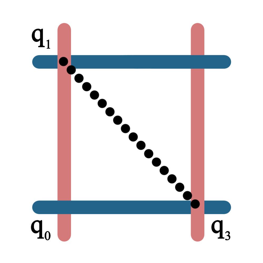
Figure 19: Treat a square hold in 4 segments as two triangles.

To apply wind force to the surface of the cloth, we need to compute an area-based force. Every square composed of four segments can be split into two triangles when computing wind force( shown in 19). The wind force has three properties affecting its influence on the cloth: velocity $\mathbf{v}_{w}$, density $\rho_{w}$, and drag $d_{w}$. $\mathbf{v}_{w}=(0,5,0)$, density $\rho_{w}=2$, and drag $d_{w}=0.5$. The wind force imposed on a triangle face $[\mathbf{q}_{0},\mathbf{q}_{1},\mathbf{q}_{3}]$ is:

$$\mathbf{F}_{w}=\rho_{w}a|v_{n}|v_{n}\mathbf{n}_{f}+d_{w}\mathbf{v}_{t}$$ (68)

where $a$ is face area, $\mathbf{n}_{f}$ is face normal, and

$$v_{n}=\mathbf{n}_{f}\left(\mathbf{v}_{w}-\frac{\dot{\mathbf{x}}_{0}+\dot{\mathbf{x}}_{1}+\dot{\mathbf{x}}_{3}}{3}\right)\mbox{,}$$

$$\mathbf{v}_{t}=\frac{\dot{\mathbf{x}}_{0}+\dot{\mathbf{x}}_{1}+\dot{\mathbf{x}}_{3}}{3}-v_{n}\mathbf{n}_{f}\mbox{.}$$

The forces on the nodes are

$$\mathbf{F}_{\mathbf{x}_{0}}=\mathbf{F}_{\mathbf{x}_{1}}=\mathbf{F}_{\mathbf{x}_{3}}=\frac{1}{3}\mathbf{F}_{w}\mbox{.}$$ (69)

B.12 Collision Response

We adopt a collision handling method originally designed for triangular meshes stored in bounding volume hierarchy (Tang et al., 2010) where continuous collision detection (CCD) can detect edge-edge and vertex-face collision. The detected vertices, edges, and faces are grouped into non-rigid impact zones (Harmon et al., 2008) for computing collision response. We treat collision response as a constrained optimization problem to prevent penetrations (Liang et al., 2019):

$$\underset{z}{\text{minimize}} \frac{1}{2}(\mathbf{x}_{colli}-\mathbf{x})^{\top}\mathbf{W}(\mathbf{x}_{colli}-\mathbf{x})$$

subject to $$\mathbf{Gx}_{colli}+\mathbf{h}\leq\mathbf{0}$$

where $\mathbf{W}$ is a weight matrix, $\mathbf{x}$ is the Lagrangian part of $\mathbf{q}$, $\mathbf{x}_{colli}$ is the updated $\mathbf{x}$ where no collision can be detected. $G$ and $h$ are constraint parameters. We assume neither self-collision nor cloth-object collision can generate considerable yarn-sliding motions, so we exclude the Eulerian terms.

Appendix C Derivatives of the simulator

Now we have a fully differentiable cloth simulator. We then compute the loss $\mathcal{L}$ that indicates the difference between the predicted and ground truth cloth states. The loss gradients with respect to the parameters $\frac{\partial\mathcal{L}}{\partial w}$ can help learn the right physics parameters via back-propagation. For simplicity, we use $\mathbf{A\dot{q}=b}$ to represent Equation 8. The differential of $\mathbf{A\dot{q}=b}$ is (Magnus & Neudecker, 2019):

$$\mathbf{A}\mathsf{d}\dot{\mathbf{q}}=\mathsf{d}\mathbf{b}-\mathsf{d}\mathbf{A}\dot{\mathbf{q}}$$ (70)

We can form the Jacobians of $\dot{\mathbf{q}}$ with respect to $\mathbf{A}$ or $\mathbf{b}$ with Equation 70. For example, to compute the $\frac{\partial\dot{\mathbf{q}}}{\partial\mathbf{A}}$, we need to set $\mathsf{d}\mathbf{A}=\mathbf{I}$ and $\mathsf{d}\mathbf{b}=\mathbf{0}$, then solve the equation and the result is $\frac{\partial\dot{\mathbf{q}}}{\partial\mathbf{A}}$. As pointed out by Amos & Kolter (2017), it is unnecessary to explicitly compute these Jacobians in back-propagation. We want to compute the product of the vector passed from back-propagation, $\frac{\partial\mathcal{L}}{\partial\dot{\mathbf{q}}}$ and the Jacobians of $\dot{\mathbf{q}}$, i.e.$\frac{\partial\mathcal{L}}{\partial\dot{\mathbf{q}}}\frac{\partial\dot{\mathbf{q}}}{\partial\mathbf{A}}$ and $\frac{\partial\mathcal{L}}{\partial\dot{\mathbf{q}}}\frac{\partial\dot{\mathbf{q}}}{\partial\mathbf{b}}$. Assume $\mathbf{A}\in\mathbb{R}^{3\times 3}$, $\dot{\mathbf{q}}\in\mathbb{R}^{3}$, and $\mathbf{b}\in\mathbb{R}^{3}$, then

$$\frac{\partial\mathcal{L}}{\partial\mathbf{b}}=\frac{\partial\mathcal{L}}{\partial\dot{\mathbf{q}}}\frac{\partial\dot{\mathbf{q}}}{\partial\mathbf{b}}=\left(\begin{pmatrix}\frac{\partial\mathcal{L}}{\partial\dot{\mathbf{q}}_{1}}&\frac{\partial\mathcal{L}}{\partial\dot{\mathbf{q}}_{2}}&\frac{\partial\mathcal{L}}{\partial\dot{\mathbf{q}}_{3}}\end{pmatrix}\begin{pmatrix}\frac{\partial\dot{\mathbf{q}}_{1}}{\partial\mathbf{b}_{1}}&\frac{\partial\dot{\mathbf{q}}_{1}}{\partial\mathbf{b}_{2}}&\frac{\partial\dot{\mathbf{q}}_{1}}{\partial\mathbf{b}_{3}}\\ \frac{\partial\dot{\mathbf{q}}_{2}}{\partial\mathbf{b}_{1}}&\frac{\partial\dot{\mathbf{q}}_{2}}{\partial\mathbf{b}_{2}}&\frac{\partial\dot{\mathbf{q}}_{2}}{\partial\mathbf{b}_{3}}\\ \frac{\partial\dot{\mathbf{q}}_{3}}{\partial\mathbf{b}_{1}}&\frac{\partial\dot{\mathbf{q}}_{3}}{\partial\mathbf{b}_{2}}&\frac{\partial\dot{\mathbf{q}}_{3}}{\partial\mathbf{b}_{3}}\end{pmatrix}\right)^{\top}$$ (71)

As

$$\frac{\partial\dot{\mathbf{q}}_{1}}{\partial\mathbf{b}_{1}}=\frac{\partial\;(\mathbf{A}^{-1})_{1,1}\mathbf{b}_{1}+(\mathbf{A}^{-1})_{1,1}\mathbf{b}_{2}+(\mathbf{A}^{-1})_{1,1}\mathbf{b}_{3}}{\partial\mathbf{b}_{1}}=\mathbf{A}^{-1}_{1,1}$$

and similarly for $\frac{\partial\mathbf{x}_{i}}{\partial\mathbf{b}_{j}}$, Equation 71 can be represented as:

$$\left(\begin{pmatrix}\frac{\partial\mathcal{L}}{\partial\dot{\mathbf{q}}_{1}}&\frac{\partial\mathcal{L}}{\partial\dot{\mathbf{q}}_{2}}&\frac{\partial\mathcal{L}}{\partial\dot{\mathbf{q}}_{3}}\end{pmatrix}\begin{pmatrix}(\mathbf{A}^{-1})_{1,1}&(\mathbf{A}^{-1})_{1,2}&(\mathbf{A}^{-1})_{1,3}\\ (\mathbf{A}^{-1})_{2,1}&(\mathbf{A}^{-1})_{2,2}&(\mathbf{A}^{-1})_{2,3}\\ (\mathbf{A}^{-1})_{3,1}&(\mathbf{A}^{-1})_{3,2}&(\mathbf{A}^{-1})_{3,3}\end{pmatrix}\right)^{\top}=(\mathbf{A}^{-1})^{\top}\frac{\partial\mathcal{L}}{\partial\dot{\mathbf{q}}}$$ (72)

After computing $\frac{\partial\mathcal{L}}{\partial\mathbf{b}}$, we need to compute $\frac{\partial\mathcal{L}}{\partial\mathbf{A}}$. The $\mathsf{}\mathbf{b}$ in Equation 70 can be set to 0 because it is irrelevant when computing $\frac{\partial\mathcal{L}}{\partial\mathbf{A}}$. Then we have

$$\mathbf{A}\mathsf{d}\dot{\mathbf{q}}=-\mathsf{d}\mathbf{A}\dot{\mathbf{q}}$$ (73)

The derivative of $\dot{\mathbf{q}}$ with respect to $\mathbf{A}_{i,j}$, the entry in the $i$th row and $j$th column of the matrix $\mathbf{A}$, is

$$\frac{\partial\dot{\mathbf{q}}}{\partial\mathbf{A}_{i,j}}=\mathbf{A}^{-1}\begin{pmatrix}\mathbf{0}\\ -\dot{\mathbf{q}}_{j}\\ \mathbf{0}\end{pmatrix}$$ (74)

According to chain rule,

$$\frac{\partial\mathcal{L}}{\partial\mathbf{A}_{i,j}}=\frac{\partial\mathcal{L}}{\partial\dot{\mathbf{q}}}\frac{\partial\dot{\mathbf{q}}}{\partial\mathbf{A}_{i,j}}=\frac{\partial\mathcal{L}}{\partial\mathbf{b}}^{\top}\mathbf{A}\mathbf{A}^{-1}\begin{pmatrix}\mathbf{0}\\ -\dot{\mathbf{q}}_{j}\\ \mathbf{0}\end{pmatrix}=-\left(\frac{\partial\mathcal{L}}{\partial\mathbf{b}}\right)_{i}\dot{\mathbf{q}}_{j}$$ (75)

The more general form is

$$\frac{\partial\mathcal{L}}{\partial\mathbf{A}}=-\frac{\partial\mathcal{L}}{\partial\mathbf{b}}\dot{\mathbf{q}}^{\top}$$ (76)

References

• Amos & Kolter (2017) Brandon Amos and J Zico Kolter. Optnet: Differentiable optimization as a layer in neural networks. In International Conference on Machine Learning, pp. 136–145. PMLR, 2017.
• Awrejcewicz (1988) J. Awrejcewicz. Chaotic motion in a nonlinear oscillator with friction. KSME Journal, 2(2):104–109, September 1988. ISSN 1738-494X. doi: 10.1007/BF02953669. URL https://doi.org/10.1007/BF02953669.
• Baraff & Witkin (1998) David Baraff and Andrew Witkin. Large steps in cloth simulation. In Proceedings of the 25th Annual Conference on Computer Graphics and Interactive Techniques, SIGGRAPH ’98, pp.  43–54, New York, NY, USA, 1998. Association for Computing Machinery. ISBN 0897919998. doi: 10.1145/280814.280821. URL https://doi.org/10.1145/280814.280821.
• Bouman et al. (2013) Katherine L Bouman, Bei Xiao, Peter Battaglia, and William T Freeman. Estimating the material properties of fabric from video. In 2013 IEEE International Conference on Computer Vision, pp. 1984–1991. IEEE, 2013. ISBN 1479928402.
• Breen et al. (1992) David E Breen, Donald H House, and Phillip H Getto. A physically-based particle model of woven cloth. The Visual Computer, 8(5):264–277, 1992.
• Cao et al. (2008) J. Cao, R. Akkerman, P. Boisse, J. Chen, H.S. Cheng, E.F. de Graaf, J.L. Gorczyca, P. Harrison, G. Hivet, J. Launay, W. Lee, L. Liu, S.V. Lomov, A. Long, E. de Luycker, F. Morestin, J. Padvoiskis, X.Q. Peng, J. Sherwood, Tz. Stoilova, X.M. Tao, I. Verpoest, A. Willems, J. Wiggers, T.X. Yu, and B. Zhu. Characterization of mechanical behavior of woven fabrics: Experimental methods and benchmark results. Composites Part A: Applied Science and Manufacturing, 39(6):1037–1053, 2008. ISSN 1359-835X. doi: https://doi.org/10.1016/j.compositesa.2008.02.016. URL https://www.sciencedirect.com/science/article/pii/S1359835X08000572.
• Casafranca et al. (2020) Juan J Casafranca, Gabriel Cirio, Alejandro Rodríguez, Eder Miguel, and Miguel A Otaduy. Mixing yarns and triangles in cloth simulation. In Computer Graphics Forum, volume 39, pp.  101–110. Wiley Online Library, 2020.
• Cirio et al. (2014) Gabriel Cirio, Jorge Lopez-Moreno, David Miraut, and Miguel A. Otaduy. Yarn-level simulation of woven cloth. ACM Trans. Graph., 33(6), November 2014. ISSN 0730-0301. doi: 10.1145/2661229.2661279. URL https://doi.org/10.1145/2661229.2661279.
• Cirio et al. (2016) Gabriel Cirio, Jorge Lopez-Moreno, and Miguel A Otaduy. Yarn-level cloth simulation with sliding persistent contacts. IEEE transactions on visualization and computer graphics, 23(2):1152–1162, 2016.
• de Avila Belbute-Peres et al. (2018a) Filipe de Avila Belbute-Peres, Kevin Smith, Kelsey Allen, Josh Tenenbaum, and J Zico Kolter. End-to-end differentiable physics for learning and control. Advances in neural information processing systems, 31:7178–7189, 2018a.
• de Avila Belbute-Peres et al. (2018b) Filipe de Avila Belbute-Peres, Kevin Smith, Kelsey Allen, Josh Tenenbaum, and J. Zico Kolter. End-to-End Differentiable Physics for Learning and Control. Advances in Neural Information Processing Systems, 31, 2018b. URL https://proceedings.neurips.cc/paper/2018/hash/842424a1d0595b76ec4fa03c46e8d755-Abstract.html.
• Degrave et al. (2019) Jonas Degrave, Michiel Hermans, Joni Dambre, et al. A differentiable physics engine for deep learning in robotics. Frontiers in neurorobotics, 13:6, 2019.
• Harmon et al. (2008) David Harmon, Etienne Vouga, Rasmus Tamstorf, and Eitan Grinspun. Robust treatment of simultaneous collisions. SIGGRAPH (ACM Transactions on Graphics), 27(3):1–4, 2008.
• Heiden et al. (2020) Eric Heiden, David Millard, Hejia Zhang, and Gaurav S. Sukhatme. Interactive Differentiable Simulation. arXiv:1905.10706 [cs, stat], May 2020. URL http://arxiv.org/abs/1905.10706. arXiv: 1905.10706.
• Hu et al. (2019) Yuanming Hu, Jiancheng Liu, Andrew Spielberg, Joshua B Tenenbaum, William T Freeman, Jiajun Wu, Daniela Rus, and Wojciech Matusik. Chainqueen: A real-time differentiable physical simulator for soft robotics. In 2019 International conference on robotics and automation (ICRA), pp.  6265–6271. IEEE, 2019.
• Huang et al. (2021) Zhiao Huang, Yuanming Hu, Tao Du, Siyuan Zhou, Hao Su, Joshua B Tenenbaum, and Chuang Gan. Plasticinelab: A soft-body manipulation benchmark with differentiable physics. arXiv preprint arXiv:2104.03311, 2021.
• James & Fatahalian (2003) Doug L. James and Kayvon Fatahalian. Precomputing interactive dynamic deformable scenes. ACM Trans. Graph., 22(3):879–887, July 2003. ISSN 0730-0301. doi: 10.1145/882262.882359. URL https://doi.org/10.1145/882262.882359.
• Jatavallabhula et al. (2021) Krishna Murthy Jatavallabhula, Miles Macklin, Florian Golemo, Vikram Voleti, Linda Petrini, Martin Weiss, Breandan Considine, Jerome Parent-Levesque, Kevin Xie, Kenny Erleben, et al. gradsim: Differentiable simulation for system identification and visuomotor control. arXiv preprint arXiv:2104.02646, 2021.
• Jawed et al. (2018) M Khalid Jawed, Alyssa Novelia, and Oliver M O’Reilly. A primer on the kinematics of discrete elastic rods. Springer, 2018.
• Johannes et al. (1973) V. I. Johannes, M. A. Green, and C. A. Brockley. The role of the rate of application of the tangential force in determining the static friction coefficient. Wear, 24(3):381–385, June 1973. ISSN 0043-1648. doi: 10.1016/0043-1648(73)90166-X. URL https://www.sciencedirect.com/science/article/pii/004316487390166X.
• Jones et al. (1998) Donald R Jones, Matthias Schonlau, and William J Welch. Efficient global optimization of expensive black-box functions. Journal of Global optimization, 13(4):455–492, 1998.
• Kaldor et al. (2008) Jonathan M Kaldor, Doug L James, and Steve Marschner. Simulating knitted cloth at the yarn level. In ACM SIGGRAPH 2008 papers, pp.  1–9. 2008.
• Kaldor et al. (2010) Jonathan M Kaldor, Doug L James, and Steve Marschner. Efficient yarn-based cloth with adaptive contact linearization. In ACM SIGGRAPH 2010 papers, pp.  1–10. 2010.
• Kim & Vendrovsky (2008) Tae-Yong Kim and Eugene Vendrovsky. Drivenshape: A data-driven approach for shape deformation. In ACM SIGGRAPH 2008 Talks, SIGGRAPH ’08, New York, NY, USA, 2008. Association for Computing Machinery. ISBN 9781605583433. doi: 10.1145/1401032.1401121. URL https://doi.org/10.1145/1401032.1401121.
• King et al. (2005) M.J. King, P. Jearanaisilawong, and S. Socrate. A continuum constitutive model for the mechanical behavior of woven fabrics. International Journal of Solids and Structures, 42(13):3867–3896, 2005. ISSN 0020-7683. doi: https://doi.org/10.1016/j.ijsolstr.2004.10.030. URL https://www.sciencedirect.com/science/article/pii/S0020768304006225.
• Lahner et al. (2018) Zorah Lahner, Daniel Cremers, and Tony Tung. Deepwrinkles: Accurate and realistic clothing modeling. In Proceedings of the European Conference on Computer Vision (ECCV), pp.  667–684, 2018.
• Li et al. (2021) Yifei Li, Tao Du, Kui Wu, Jie Xu, and Wojciech Matusik. Diffcloth: Differentiable cloth simulation with dry frictional contact. arXiv preprint arXiv:2106.05306, 2021.
• Li et al. (2019) Yunzhu Li, Jiajun Wu, Russ Tedrake, Joshua B. Tenenbaum, and Antonio Torralba. Learning Particle Dynamics for Manipulating Rigid Bodies, Deformable Objects, and Fluids. arXiv:1810.01566 [physics, stat], April 2019. URL http://arxiv.org/abs/1810.01566. arXiv: 1810.01566.
• Liang et al. (2019) Junbang Liang, Ming Lin, and Vladlen Koltun. Differentiable cloth simulation for inverse problems. 2019.
• Long et al. (2011) James Long, Katherine Burns, and Jingzhou James Yang. Cloth modeling and simulation: a literature survey. In International Conference on Digital Human Modeling, pp. 312–320. Springer, 2011.
• Loock et al. (2001) Achim Loock, Elmar Schömer, and Im Stadtwald. A virtual environment for interactive assembly simulation: From rigid bodies to deformable cables. In 5th World Multiconference on Systemics, Cybernetics and Informatics (SCI’01), volume 3, pp.  325–332. Citeseer, 2001.
• Magnus & Neudecker (2019) Jan R Magnus and Heinz Neudecker. Matrix differential calculus with applications in statistics and econometrics. John Wiley & Sons, 2019.
• Mohammed et al. (2000) U. Mohammed, C. Lekakou, L. Dong, and M.G. Bader. Shear deformation and micromechanics of woven fabrics. Composites Part A: Applied Science and Manufacturing, 31(4):299–308, 2000. ISSN 1359-835X. doi: https://doi.org/10.1016/S1359-835X(99)00081-0. URL https://www.sciencedirect.com/science/article/pii/S1359835X99000810.
• Narain et al. (2012) Rahul Narain, Armin Samii, and James F O’brien. Adaptive anisotropic remeshing for cloth simulation. ACM transactions on graphics (TOG), 31(6):1–10, 2012.
• Parsons et al. (2010) Ethan M. Parsons, Tusit Weerasooriya, Sai Sarva, and Simona Socrate. Impact of woven fabric: Experiments and mesostructure-based continuum-level simulations. Journal of the Mechanics and Physics of Solids, 58(11):1995–2021, 2010. ISSN 0022-5096. doi: https://doi.org/10.1016/j.jmps.2010.05.006. URL https://www.sciencedirect.com/science/article/pii/S0022509610000967.
• Peng et al. (2004) X.Q. Peng, J. Cao, J. Chen, P. Xue, D.S. Lussier, and L. Liu. Experimental and numerical analysis on normalization of picture frame tests for composite materials. Composites Science and Technology, 64(1):11–21, 2004. ISSN 0266-3538. doi: https://doi.org/10.1016/S0266-3538(03)00202-1. URL https://www.sciencedirect.com/science/article/pii/S0266353803002021.
• Pfaff et al. (2020) Tobias Pfaff, Meire Fortunato, Alvaro Sanchez-Gonzalez, and Peter Battaglia. Learning Mesh-Based Simulation with Graph Networks. September 2020. URL https://openreview.net/forum?id=roNqYL0_XP.
• Pizana et al. (2020) José M Pizana, Alejandro Rodríguez, Gabriel Cirio, and Miguel A Otaduy. A bending model for nodal discretizations of yarn-level cloth. In Computer Graphics Forum, volume 39, pp.  181–189. Wiley Online Library, 2020.
• Provot et al. (1995) Xavier Provot et al. Deformation constraints in a mass-spring model to describe rigid cloth behaviour. In Graphics interface, pp.  147–147. Canadian Information Processing Society, 1995.
• Rasheed et al. (2020) Abdullah-Haroon Rasheed, Victor Romero, Florence Bertails-Descoubes, Stefanie Wuhrer, Jean-Sébastien Franco, and Arnaud Lazarus. Learning to Measure the Static Friction Coefficient in Cloth Contact. In CVPR 2020 - IEEE Conference on Computer Vision and Pattern Recognition, pp.  9909–9918, Seattle, United States, June 2020. IEEE. doi: 10.1109/CVPR42600.2020.00993. URL https://hal.inria.fr/hal-02511646.
• Runia et al. (2020) Tom F H Runia, Kirill Gavrilyuk, Cees G M Snoek, and Arnold W M Smeulders. Cloth in the wind: A case study of estimating physical measurement through simulation. In The IEEE Conference on Computer Vision and Pattern Recognition (CVPR), June 2020.
• Sánchez-Banderas et al. (2020) Rosa M Sánchez-Banderas, Alejandro Rodríguez, Héctor Barreiro, and Miguel A Otaduy. Robust eulerian-on-lagrangian rods. ACM Transactions on Graphics (TOG), 39(4):59–1, 2020.
• Schenck & Fox (2018) Connor Schenck and Dieter Fox. Spnets: Differentiable fluid dynamics for deep neural networks. In Conference on Robot Learning, pp.  317–335. PMLR, 2018.
• Schulman et al. (2017) John Schulman, Filip Wolski, Prafulla Dhariwal, Alec Radford, and Oleg Klimov. Proximal policy optimization algorithms. arXiv preprint arXiv:1707.06347, 2017.
• Shen et al. (2021) Siyuan Shen, Yin Yang, Tianjia Shao, He Wang, Chenfanfu Jiang, Lei Lan, and Kun Zhou. High-order differentiable autoencoder for nonlinear model reduction. SIGGRAPH (ACM Transactions on Graphics), 40(4), August 2021.
• Snoek et al. (2012) Jasper Snoek, Hugo Larochelle, and Ryan P Adams. Practical bayesian optimization of machine learning algorithms. Advances in neural information processing systems, 25, 2012.
• Sperl et al. (2020) Georg Sperl, Rahul Narain, and Chris Wojtan. Homogenized yarn-level cloth. ACM Transactions on Graphics (TOG), 39(4):2, 2020.
• Spillmann & Teschner (2007) Jonas Spillmann and Matthias Teschner. Corde: Cosserat rod elements for the dynamic simulation of one-dimensional elastic objects. In Proceedings of the 2007 ACM SIGGRAPH/Eurographics symposium on Computer animation, pp.  63–72, 2007.
• Stribeck (1902) Richard Stribeck. Die wesentlichen eigenschaften der gieit-und rollenlager–the key qualities of sliding and roller bearings. Zeitschrift des Vereines Seutscher Ingenieure, 46(38):1342–1348, 1902.
• Sueda et al. (2011) Shinjiro Sueda, Garrett L. Jones, David I. W. Levin, and Dinesh K. Pai. Large-scale dynamic simulation of highly constrained strands. ACM Trans. Graph., 30(4), July 2011. ISSN 0730-0301. doi: 10.1145/2010324.1964934. URL https://doi.org/10.1145/2010324.1964934.
• Sullivan (2008) John M Sullivan. Curves of finite total curvature. In Discrete differential geometry, pp.  137–161. Springer, 2008.
• Tang et al. (2010) Min Tang, Dinesh Manocha, and Ruofeng Tong. Fast continuous collision detection using deforming non-penetration filters. In Proceedings of the 2010 ACM SIGGRAPH Symposium on Interactive 3D Graphics and Games, I3D ’10, pp.  7–13, New York, NY, USA, 2010. Association for Computing Machinery. ISBN 9781605589398. doi: 10.1145/1730804.1730806. URL https://doi.org/10.1145/1730804.1730806.
• Wang et al. (2011) Huamin Wang, James F O’Brien, and Ravi Ramamoorthi. Data-driven elastic models for cloth: modeling and measurement. ACM transactions on graphics (TOG), 30(4):1–12, 2011.
• Wang et al. (1999) J. Wang, R. Paton, and J.R. Page. The draping of woven fabric preforms and prepregs for production of polymer composite components. Composites Part A: Applied Science and Manufacturing, 30(6):757–765, 1999. ISSN 1359-835X. doi: https://doi.org/10.1016/S1359-835X(98)00187-0. URL https://www.sciencedirect.com/science/article/pii/S1359835X98001870.
• Wang et al. (2020) Kun Wang, Mridul Aanjaneya, and Kostas Bekris. A First Principles Approach for Data-Efficient System Identification of Spring-Rod Systems via Differentiable Physics Engines. In Learning for Dynamics and Control, pp.  651–665. PMLR, July 2020. URL http://proceedings.mlr.press/v120/wang20b.html. ISSN: 2640-3498.
• Yang et al. (2017a) Shan Yang, Junbang Liang, and Ming C Lin. Learning-based cloth material recovery from video. In 2017 IEEE International Conference on Computer Vision (ICCV), pp.  4393–4403. IEEE, 2017a. ISBN 9781538610329.
• Yang et al. (2017b) Shan Yang, Junbang Liang, and Ming C Lin. Learning-based cloth material recovery from video. In Proceedings of the IEEE International Conference on Computer Vision, pp.  4383–4393, 2017b.
• Zhong et al. (2021) Yaofeng Desmond Zhong, Biswadip Dey, and Amit Chakraborty. A Differentiable Contact Model to Extend Lagrangian and Hamiltonian Neural Networks for Modeling Hybrid Dynamics. arXiv:2102.06794 [cs], February 2021. arXiv: 2102.06794.
• Zhou et al. (2017) Yi Zhou, Muhammad Ali, Xiaozhou Gong, and Dan Yang. An overview of yarn pull-out behavior of woven fabrics. Textile Research Journal, 89:004051751774115, November 2017. doi: 10.1177/0040517517741156.