EPHS: A Port-Hamiltonian Modelling Language

Abstract

A prevalent theme throughout science and engineering is the ongoing paradigm shift away from isolated systems towards open and interconnected systems. Port-Hamiltonian theory developed as a synthesis of geometric mechanics and network theory. The possibility to model complex multiphysical systems via interconnection of simpler components is often advertised as one of its most attractive features. The development of a port-Hamiltonian modelling language however remains a topic which has not been sufficiently addressed. We report on recent progress towards the formalization and implementation of a modelling language for exergetic port-Hamiltonian systems. Its diagrammatic syntax inspired by bond graphs and its functorial semantics together enable a modular and hierarchical approach to model specification.

1 Introduction

Mathematical modelling of physical systems and the closely related fields of computer simulation, optimization, and control keep growing in their importance for scientific discovery and the design and operation of engineered systems. Although compositional thinking is prevalent throughout science and engineering, modelling and simulation software is still lacking in this respect. Contrary to reality, models are often restricted to isolated systems and model specifications are often intermingled with the computational procedures used to evaluate them.

The advent of equation-based modelling languages like Modelica has improved the situation by offering a declarative approach: Components are defined by their time-dependent variables, parameters, connectors, and the equations relating the former. Hierarchical models can be defined by instantiating components and connecting them via their connectors. The compiler turns model specifications into (hybrid) systems of differential-algebraic equations (DAEs) and uses structural simplification algorithms to make them amenable to numerical methods for simulation, see Modelica Association (2021).

Some limitations however prompt us to think that future tools for modelling physical systems might have to rely on a different kind of language: While Modelica and similar languages offer a practical way to write down systems of DAEs, they lack the ability to express models with more abstract semantics such as those defined via partial differential(-algebraic) equations stated within the vector or exterior calculus formalism. Further, these languages are unable to directly express and assert the structural properties inherent to all models of physical systems. This structure can be made manifest via the Port-Hamiltonian Systems (PHS) framework, see Sec. 2.1. Despite of successful efforts to integrate the PHS framework with Modelica, see Marquez et al. (2020), we want to formalize a new language specifically tailored towards expressing (lumped- and distributed-parameter) port-Hamiltonian semantics in a simple and mathematically rigorous manner. We seek a language which conveys the physical and compositional structure at a level above the defining equations, where it can be exploited more easily for the purpose of analysis, model transformations, simulation, optimization, control, and scientific machine learning.

The present paper is concerned with the formalization of a language for composable networks of multiphysical and thermodynamic systems within the Exergetic Port-Hamiltonian Systems (EPHS) framework, see Lohmayer et al. (2021). Due to its intuitive diagrammatic syntax, the proposed language could form a basis for novel computer-aided engineering (CAE) tools as well as facilitate interdisciplinary communication, decision making, and education. A close connection to the exergy analysis method makes the language particularly interesting for thermodynamic optimization and sustainable engineering.

Throughout science and engineering, various sorts of diagrams, such as circuit diagrams, block diagrams, and Petri nets, are employed to depict information about mathematical models. In applied category theory research, the formalization of such diagrams based on monoidal categories and their underlying operads has been a major topic, see e.g. Baez and Erberle (2015); Baez and Pollard (2017); Baez and Fong (2018); Baez et al. (2021); Bakirtzis et al. (2021) and references therein. We focus on the operadic perspective because it is much closer to how we visually express and implement the language. An operad is a mathematical object used to organize formal ‘operations’ which have finitely many ‘inputs’ and one ‘output’. An operad algebra then endows the formal operations with semantics. One speaks of a coloured operad when its operations compose only if their respective inputs and outputs have matching types, see Leinster (2004); Yau (2016). We shall make use of the operad of undirected wiring diagrams which initially appeared in Spivak (2013) together with its relational algebra used to model database queries, see also Spivak (2014); Yau (2018); Breiner et al. (2020). The recent paper by Libkind et al. (2021) deals with an operadic approach to modelling of discrete and continuous dynamical systems with directed and undirected semantics of composition and its software implementation.

Relying on the operad of undirected wiring diagrams, we can give a precise definition of a diagrammatic syntax for (exergetic) port-Hamiltonian systems which has a close connection to bond graphs. Further, we can formalize different kinds of (exergetic) port-Hamiltonian semantics as an algebra over this operad.

To make the paper as self-contained as possible, in Sec. 2 we review some concepts from port-Hamiltonian systems and category theory. In Sec. 3 we introduce the syntax of the proposed modelling language from an intuitive standpoint and then go on to show how it can be formalized based on the operad of undirected wiring diagrams. Finally we briefly mention how to assign semantics. In Sec. 4 we state our conclusions and give an outlook on future work.

2 Background

We introduce mostly via example necessary concepts from (exergetic) port-Hamiltonian systems and category theory.

2.1 Port-Hamiltonian Systems

For didactic purposes, we consider one of the simplest examples: A damped harmonic oscillator features a spring, a moving mass and a damper. The stored energy is expressed via the Hamiltonian function $H$ defined by

$$H(q,p)\>=\>E_{\text{spring}}(q)+E_{\text{mass}}(p)\>=\>\frac{1}{2\,c}\,q^{2}+\frac{1}{2\,m}\,p^{2}\,.$$ (1)

The extension $q$ and the momentum $p$ are state variables, while the compliance $c$ and the mass $m$ are fixed parameters. The centrepiece of a port-Hamiltonian system (PHS) is its Dirac structure which can be defined via a skew-symmetric matrix encoding the power-conserving interconnection:

$$\left[\begin{array}[]{c}\dot{q}\\ \dot{p}\\ \hline\cr e_{Rm}\end{array}\right]\>=\>\left[\begin{array}[]{rr|r}0&1&0\\ -1&0&-1\\ \hline\cr 0&1&0\end{array}\right]\,\left[\begin{array}[]{c}\partial_{q}H\\ \partial_{p}H\\ \hline\cr f_{Rm}\end{array}\right]$$ (2)

The damping is expressed through a resistive relation $\mathcal{R}$ which relates the flow and effort variables of the third port:

$$f_{Rm}\>=\>d\,e_{Rm}$$ (3)

The Dirac structure implies the power-balance equation

$$\partial_{t}\bigl{(}H(q(t),p(t))\bigr{)}\>+\>e_{Rm}(t)\,f_{Rm}(t)\>=\>0$$ (4)

which says that the net discharge of the stored energy equals the power which is ‘dissipated’ in the damper. According to our sign convention, the stored power, the dissipated power, and the power supplied via additional boundary ports sum to zero. If the Hamiltonian is bounded from below, the system is said to be passive. The ways how components of a model can exchange power is often expressed schematically as a bond graph:

$\mathcal{D}$ represents the Dirac structure, $\mathbb{C}$ (like capacitor) symbolizes storage, and $\mathbb{R}$ (like resistor) stands for dissipation.

We refer to van der Schaft and Jeltsema (2014) for a more in-depth introduction to port-Hamiltonian systems.

2.2 Exergetic Port-Hamiltonian Systems

The EPHS framework establishes a more rigorous thermodynamic foundation for PHS: Rather than energy, the central notion is exergy, a quantity which indeed is dissipated in thermodynamic systems. Its definition relies on a (reference) environment which serves to quantify the degradation of energy. It further acts as an isothermal reservoir which can absorb waste heat and as an isobaric atmosphere, etc. The word ‘environment’ thus acquires a meaning quite different from ‘other systems’.

In place of (3), the resistive structure is defined by

$$\left[\begin{array}[]{c}f_{Rm}\\ f_{Rt}\end{array}\right]\>=\>\frac{1}{\theta_{0}}\,d\,\left[\begin{array}[]{rr}\theta_{0}&-\upsilon\\ -\upsilon&\upsilon^{2}/\theta_{0}\end{array}\right]\,\left[\begin{array}[]{c}e_{Rm}\\ e_{Rt}\end{array}\right]\,,$$ (5)

where $\upsilon:=p/m=e_{Rm}$ is the velocity of the mass and $\theta_{0}$ is the fixed reference temperature of the environment. It relates the mechanical port with an additional thermal port in an energy-conserving, yet dissipative, i.e. entropy producing, manner. The symmetry of the above matrix is related to Onsager’s reciprocal relations. Its positive semidefiniteness encodes non-negative entropy production and its non-trivial kernel encodes conservation of energy. To express the disposal of waste heat, the thermal port is connected to the environment via an extension of the Dirac structure:

$$\left[\begin{array}[]{c}\dot{s}_{e}\\ \hline\cr e_{Rt}\end{array}\right]\>=\>\left[\begin{array}[]{r|r}0&-1\\ \hline\cr 1&0\end{array}\right]\,\left[\begin{array}[]{c}0\\ \hline\cr f_{Rt}\end{array}\right]$$ (6)

Here, $s_{e}$ is the entropy state variable of the environment. The effort variable corresponding to $\dot{s}_{e}$ is $0$ because heat exchanged with the environment has no exergetic value. Eqs. (1), (2), (5), (6) defining the EPHS reduce to $\dot{q}=\upsilon$, $\dot{p}=-\frac{1}{c}\,q-d\,\upsilon$, and $\dot{s}_{e}=\frac{1}{\theta_{0}}\,d\,\upsilon^{2}$. Even though this is more concise, it is less amenable to analysis. The structured representation brings to light the inherent properties of thermodynamic systems, first and foremost conservation of energy and non-negative entropy production. Passivity is tantamount to stability of the thermodynamic equilibrium state. We refer to Lohmayer et al. (2021) for more details.

2.3 Category Theory

A category has objects and (homo)morphisms also called arrows. We write $\mathrm{Ob}(C)$ for the set of objects of the (small) category $C$ and for any $x,\,y\in\mathrm{Ob}(C)$ we write $\mathrm{Hom}(x,\,y)$ for the set of morphisms with domain object $x$ and codomain object $y$, i.e. for arrows from $x$ to $y$. Morphisms compose associatively. For $f\in\mathrm{Hom}(x,\,y)$ and $g\in\mathrm{Hom}(y,\,z)$ there exists $g\circ f\in\mathrm{Hom}(x,\,y)$. For every $x\in\mathrm{Ob}(C)$, there exists a designated morphism $\mathrm{id}_{x}\in\mathrm{Hom}(x,x)$ which behaves as an identity with respect to (pre- and post-)composition. We write this as the diagram

$$\leavevmode\hbox to89.9pt{\vbox to13.67pt{\text{[drawing]}}}. {x} {y} {z} \scriptstyle{f} \scriptstyle{g} {x} {y} {z} \scriptstyle{f} \scriptstyle{g}$$

Composite and identity morphisms are usually omitted because their existence is guaranteed by the axioms. Every directed graph can be made into a category with vertices as objects and edges as morphisms. Identity and composite morphisms must be (freely) added. String diagrams are (Poincaré) dual to diagrams such as the above and provide a formal syntax for morphisms in (monoidal) categories:

Objects and their identity morphisms are drawn as strings (edges), and the morphisms are drawn as boxes (nodes). An import (small) category is $\mathrm{FinSet}$ whose objects are finite sets and whose morphisms are functions between them. There is also a category $\mathrm{Set}$ of (‘small’ but not necessarily finite) sets and functions between them. (This category is not small because its objects do not form a set.) A functor is a structure-preserving map between categories. If $C$ and $D$ are categories, a functor $F:C\rightarrow D$ maps an object $x\in\mathrm{Ob}(C)$ to an object $F(x)\in\mathrm{Ob}(D)$ and maps a morphism $f\in\mathrm{Hom}_{C}(x,\,y)$ to a morphism $F(f)\in\mathrm{Hom}_{D}(F(x),\,F(y))$. A construction is functorial if it can be expressed as a map between categories which preserves composition and identity. A prominent example is the tangent functor which maps the category of smooth manifolds to the category of smooth vector bundles. It sends a manifold to its tangent bundle and it sends a map between manifolds to its linearisation. Functoriality is tantamount to the chain rule, i.e. the linearisation of a composite is equal to the composite of the linearisations.

Multicategories generalize categories by allowing morphisms with finitely many domain objects. A multicategory is called symmetric if permuting the order of the domain objects plays together nicely with composition. Symmetric multicategories are also called coloured operads but we will henceforth just say operads. Objects are thought of as the input and output types of formal $n$-ary operations ($n\in\mathbb{N}$) which constitute the morphisms. If $a,\,b,\,c,\,d,\,e\in\mathrm{Ob}(O)$ are objects of an operad $O$ and $f\in\mathrm{Hom}(a,\,b;\,c)$, $g\in\mathrm{Hom}(c,\,d;\,e)$ are morphisms then the composite $g\circ\left(f,\,\mathrm{id}_{d}\right)\in\mathrm{Hom}(a,\,b,\,d;\,e)$ corresponds to the following string diagram:

$$\begin{gathered}\includegraphics[width=142.26378pt]{string_diagrams/string_diagram_multicategory.eps}\end{gathered}$$ (7)

The objects of the operad $\mathrm{Sets}$ are the (small) sets and its morphisms are all $n$-any functions between them. Functors between operads are defined in essentially the same way. The formal operations of an operad $O$ can be endowed with semantics via a functor $F:O\rightarrow\mathrm{Sets}$ called an algebra over $O$. $F$ sends an object (type) to the set which contains the elements of that type and it sends a morphism (formal operation) to the function which acts on elements of the respective types in the desired way (i.e. its meaning or implementation). The semantics are functorial because assigning concrete meaning to formal operations plays together nicely with their composition.

While Mac Lane (1998) provides an introduction to category theory for mathematicians, Spivak (2014) addresses a general scientific audience and also includes a section on operads and their algebras. Operads are thoroughly treated in Leinster (2004) and Yau (2016). Operads of wiring diagrams are extensively covered in Yau (2018).

3 Modelling language

Due to their structural properties, PHS are considered attractive for analysis and control. EPHS in particular are well suited for multiphysics applications. Therefore we ask what is missing to bring PHS to engineering teams? Although often advertised, the potential of the framework for such enterprise remains unrealized. Hoping to make some progress on this front, we discuss EPHS as a modelling language, a topic beyond ‘equations with geometric structure and thermodynamic interpretation’.

Modelling paradigms are often classified as top-down vs. bottom-up. PHS enable a bottom-up approach, since relatively simple systems can be interconnected to form more complex ones. We advocate an operadic approach which perhaps has more of a top-down flavour: We argue that modelling of a physical system starts with its decomposition, yielding an account not only of its parts but also of their interconnection. Parts can be decomposed recursively until all low-level parts are sufficiently simple, making it relatively straightforward to associate to them their precise meaning. The structure behind hierarchical decompositions of systems into interconnected parts is called the syntax of the modelling language. The structure which governs how meaning, in the form of equations or related data structures, is associated to decompositions is called semantics. Note that we could also conceive of this as a bottom-up approach: A syntactic expression then represents the composition pattern of a system which can be a part of a another composition pattern, etc.

It seems rather self-evident that some sort of bond graphs should be used as a formal syntax for PHS. However, as such, bond graphs are not mathematical objects. Most researchers probably think of them as directed graphs, see e.g. Pfeifer et al. (2020). In Coya (2017) a categorical framework is presented featuring $0$- and $1$-junctions as syntax and functorial semantics for the thereby expressed junction structure. We propose a categorical framework with a syntax using only $0$-junctions, yet arbitrary Dirac structures can be included via semantics: A (bond-graph) expression which can be used to define an isothermal oscillator is shown in Fig. 1.

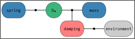
Figure 1: Bond-graph expression for defining an EPHS model of an isothermal damped harmonic oscillator.

The ‘outer box’ is interpreted as the boundary of the represented composite system. The (inner) ‘boxes’ are drawn with rounded corners or as circles and represent the system components. Boxes expose ‘ports’ which are connected via ‘bonds’ drawn as lines to ‘junctions’ drawn as black circles. The junctions and the box named $\texttt{D}_{\texttt{m}}$ define the Dirac structure. The latter connects the potential energy domain on its left with the kinetic energy domain on its right. The junction at the bottom right belongs to the thermal energy domain.

The operad structure allows us to compose bond-graph expressions. This can be understood as substitution of one expression into another. To define a nonisothermal oscillator, we need to include the thermal capacity of the damper as well as a heat transfer law governing its cool-down.

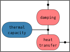
Figure 2: Bond-graph expression for defining an EPHS model of a non-isothermal damper.

The model refinement can proceed by substituting the expression shown in Fig. 2 into the box labelled damping in the expression shown in Fig. 1. The outer box of the substituted expression has two ‘boundary ports’ because it represents an open system.

A box together with its ports is understood as the interface of the component that it represents. Composition proceeds via identification of interfaces: The outer box in the substituted expression is identified with the box into which it is substituted. The resulting composite expression is shown in Fig. 3. The shared interface disappears and for each of its ports, the two corresponding junctions, one on either side of the interface, are also identified.

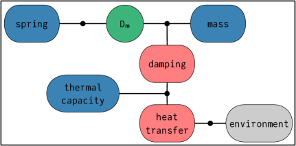
Figure 3: Bond-graph expression for defining an EPHS model of a non-isothermal oscillator.

Bonds and their junctions represent the power-conserving interconnection of components. At every junction the flow variables of all incident bonds sum to zero while the corresponding effort variables are equal. We fix that power going into any (outer) box has a positive sign, making arrowheads on bonds unnecessary. This leads to a much simpler formalism and less visual noise. Stored power, dissipated power, and supplied power is hence associated with a positive sign.

While junctions incident to exactly two bonds might seem unnecessary at first, they are required to formalize a simple and composable syntax. Further, they are convenient from the perspective of a graphical user interface (GUI) for manipulating bond-graph expressions. Junctions with one incident bond define physically meaningful constraints.

Traditional bond graphs also feature $1$-junctions, where efforts sum to zero and flows are equal. While they can be represented by boxes via semantics, they seem unnecessary due to the different roles of flow and effort variables in the EPHS framework. Flow variables are related to rates of extensive quantities or thermodynamic fluxes, while effort variables are related to intensive quantities or thermodynamic forces.

Boxes are identified via their labels. Although part of an expression, we chose to omit labels for (boundary) ports in their visual representation. In contrast, junctions do not have labels.

We further omit that ports and junctions have a type corresponding to the physical dimensions of their port variables. The interconnection of components as captured by expressions and the operadic composition of expressions involve automatic type checking. Semantic data defining a low-level component may further include type annotations which are checked against its interface.

Although boxes do not have a colour at the level of syntax, we hint at the associated semantics by drawing them with a white filling if they represent a nested EPHS. Similarly, blue for exergy storage, green for Dirac structure, red for resistive structure, and grey for the reference environment.

An expression can be understood as defining an operation which takes the meaning of each inner box and returns the meaning of the outer box. For instance, the expression shown in Fig. 4 has two boundary ports.

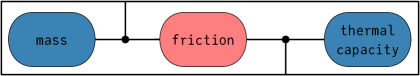
Figure 4: Bond-graph expression for defining an EPHS model of a moving piston with friction.

Hence, if we provide appropriate meaning for its three boxes we get the meaning of the composite system. If we then take this as the meaning of the box labelled piston in Fig. 5

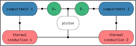
Figure 5: Bond-graph expression for defining an EPHS model of a cylinder-piston device.

and fix an appropriate meaning for the other five boxes, we obtain the model of the isolated piston-cylinder device of Example 5.4 in Lohmayer et al. (2021). $\texttt{D}_{\texttt{+}}$ and $\texttt{D}_{\texttt{-}}$ interconnect the kinetic port of the piston and the port for pressure-volume work of either compartment, taking into account the cross-sectional area of the cylinder. The two Dirac structures differ in sign, since compartment pressure acts on the piston from different sides. If we would first compose the expressions shown in Fig. 4 and 5, i.e. substitute the former expression into the box labelled piston in the latter expression, and then fix the meaning of all boxes in the composite expression accordingly, we would obtain the same model due to functoriality of the semantics.

The environment has a special singleton role. It is part of every system in order to define its exergy and at the same time it may be represented by any number of boxes, including zero, as in the previous example.

The operadic approach allows us to hierarchically define and refine models. It also allows us to reuse expressions either with or without meaning associated to their boxes. We obtain the model of the heated piston-cylinder device of Example 5.6 in Lohmayer et al. (2021) if we reuse parts from the definition of the previous examples to fix the meaning of the expression shown in Fig. 6. Only the resistor needs to be modelled additionally.

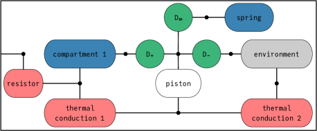
Figure 6: Bond-graph expression for defining an EPHS model of a heated cylinder-piston device.

In Lohmayer et al. (2021) we used a different syntax, see Fig. 7.

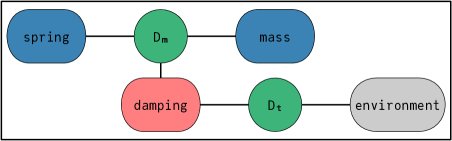
Figure 7: Bond-graph expression for defining an EPHS model of an isothermal damped harmonic oscillator based on the syntax used in Lohmayer et al. (2021).

It is remarkable that the change required to make the syntax compatible with the operadic structure also brings other benefits, namely a clearer separation of physical domains and specification of the Dirac structure with fewer boxes.

3.1 Syntax

The syntax is formalized as the operad of typed undirected wiring diagrams $\mathrm{UWD}$, see Spivak (2013) and Yau (2018). It has boxes as objects and wiring diagrams (i.e. bond-graph expressions) as morphisms. A box is a finite set of ports $b$ with a function $\tau_{b}$ assigning to each port its type:

$$\mathrm{Ob}(\mathrm{UWD})=\{\left(b,\,\tau_{b}\right)\mid b\in\mathrm{Ob}(\mathrm{FinSet}),\,\tau_{b}\colon b\rightarrow\mathrm{Ob}(\mathrm{Set})\}$$

For instance, the box $b=\{p_{1},p_{2}\}$ comes with a function $\tau_{b}$ defined by $\tau_{b}(p_{1})=P_{1}$, $\tau_{b}(p_{2})=P_{2}$. We think of a port type as the set of values of flow and effort variables whose physical dimensions match the physical domain to which the respective port belongs. The box can be drawn like so:

A morphism $f$ is a formal $n$-ary operation with domain objects or inner boxes $b_{i}$ ($i=1,\,\ldots,\,n$) and codomain object or outer box $b_{o}$, i.e. $f\in\mathrm{Hom}(b_{1},\,\ldots,\,b_{n};\,b_{o})$. For instance, the morphism $g$ in Eq. (7) represents a system with boundary ports given by the set $e$ and two inner boxes with ports given by the sets $c$ and $d$, respectively. The composite morphism $g\circ\left(f,\,\mathrm{id}_{d}\right)$ represents a system with boundary ports given by $e$ and three inner boxes with ports given by $a$, $b$, and $d$, respectively. The data of a $n$-ary morphism, i.e. a bond-graph expression with $n$ inner boxes, is defined by a commutative diagram of the form

The coproduct $\coprod_{i}b_{i}$ is the disjoint union of the ports of all inner boxes. The functions $\mathrm{j}_{\mathrm{i}}$ and $\mathrm{j}_{\mathrm{o}}$ are morphisms in $\mathrm{FinSet}$ and assign ports to junctions. To express that junctions are not labelled we can define morphisms as equivalence classes of diagrams as the above. However, this seems unnecessary for software implementation.

In the following we ignore the type information for brevity. Given a box $b$, the identity on $b$ is defined by the diagram $b\rightarrow b\leftarrow b$ with two identity morphisms in $\mathrm{FinSet}$.

Given $g\in\mathrm{Hom}(b_{1},\,\ldots,\,b_{n};\,b_{o})$ defined by

for some $n\in\mathbb{N}$ and for each $i\in\{1,\,\ldots,\,n\}$ a morphism $f_{i}\in\mathrm{Hom}(b_{i,1},\,\ldots,\,b_{i,m_{i}};\,b_{i})$ defined by

for some $m_{i}\in\mathbb{N}$, the composite $g\circ\left(f_{i},\,\ldots,\,f_{n}\right)\in\mathrm{Hom}(b_{1,1},\,\ldots,\,b_{n,m_{n}};\,b_{o})$ is defined (via pushout) by

with $\mathrm{i}_{\mathrm{i}}\circ\left(\coprod_{i}\mathrm{j}_{\mathrm{i}}^{f_{i}}\right)$ and $\mathrm{i}_{\mathrm{o}}\circ\mathrm{j}_{\mathrm{o}}^{g}$ as the two defining functions. The junctions $J$ of the composite wiring diagram together with injections $\mathrm{i}_{\mathrm{i}}$ and $\mathrm{i}_{\mathrm{o}}$ are determined via the commuting (pushout) square. The ports of the shared interfaces $\coprod_{i}b_{i}$ determine which junctions in $J$ are identified.

Attributed C-Sets are defined in Patterson et al. (2021b) and provide a categorical framework for defining data structures for graph-like objects with data attributes. The framework is implemented in the Julia programming language, see Patterson et al. (2021a). Ignoring attributes, a $C$-Set is a functor from a category $C$ to $\mathrm{FinSet}$. The combinatorial data of a bond-graph expression can be expressed as such a functor with the (free) category $C$ defined by the black part of

Similarly, the violet part is mapped to the data attributes encoding the port types.

3.2 Semantics

The semantics of the modelling language is formalized as an algebra over $\mathrm{UWD}$, i.e. as a functor to the operad $\mathrm{Sets}$. On objects, it sends a box to the set of EPHS with boundary ports matching the interface defined by the box. On $n$-ary morphisms, it sends a bond-graph expression with $n$ inner boxes to a function which takes $n$ EPHS matching the inner boxes and returns an EPHS matching the outer box. A bond-graph expression hence defines a function that composes port-Hamiltonian systems. Every box in the defining expression corresponds to a function argument. Regarding the precise definition of this functor, the unique role of the environment deserves special attention. We defer details of this construction to later.

4 Conclusion

We introduce a formal modelling language which focuses on expressing physical and compositional structure, rather than merely systems of equations. In particular, we show that a diagrammatic syntax inspired by bond graphs can be formalized based on the operad of typed undirected wiring diagrams. This work can form the basis of valuable software tools for researchers working on port-Hamiltonian systems theory. Eventually, it could also bring port-Hamiltonian systems closer to real-world applications.

Future work on the exergetic port-Hamiltonian systems framework will focus on presenting a complete definition of the semantics and on a software implementation of the modelling language. We also plan to work on the integration of the modelling language with distributed-parameter models and physics-informed machine learning.

References

- Baez and Erberle (2015) Baez, J. and Erberle, J. (2015). Categories in control. Theory and Applications of Categories, 30(24), 836–881.
- Baez et al. (2021) Baez, J.C., Courser, K., and Vasilakopoulou, C. (2021). Structured versus decorated cospans.
- Baez and Fong (2018) Baez, J.C. and Fong, B. (2018). A compositional framework for passive linear networks.
- Baez and Pollard (2017) Baez, J.C. and Pollard, B.S. (2017). A compositional framework for reaction networks. Reviews in Mathematical Physics, 29(09), 1750028. 10.1142/s0129055x17500283.
- Bakirtzis et al. (2021) Bakirtzis, G., Vasilakopoulou, C., and Fleming, C.H. (2021). Compositional cyber-physical systems modeling. In Proceedings of Applied Category Theory (ACT2020), volume 333, 125–138. Open Publishing Association. 10.4204/eptcs.333.9.
- Breiner et al. (2020) Breiner, S., Pollard, B., Subrahmanian, E., and Marie-Rose, O. (2020). Modeling hierarchical system with operads. Electronic Proceedings in Theoretical Computer Science, 323, 72–83. 10.4204/eptcs.323.5.
- Coya (2017) Coya, B. (2017). A compositional framework for bond graphs.
- Leinster (2004) Leinster, T. (2004). Higher Operads, Higher Categories. London Mathematical Society Lecture Note Series. Cambridge University Press. 10.1017/CBO9780511525896.
- Libkind et al. (2021) Libkind, S., Baas, A., Patterson, E., and Fairbanks, J. (2021). Operadic modeling of dynamical systems: Mathematics and computation.
- Lohmayer et al. (2021) Lohmayer, M., Kotyczka, P., and Leyendecker, S. (2021). Exergetic port-Hamiltonian systems: modelling basics. Mathematical and Computer Modelling of Dynamical Systems, 27(1), 489–521. 10.1080/13873954.2021.1979592.
- Mac Lane (1998) Mac Lane, S. (1998). Categories for the Working Mathematician. Graduate Texts in Mathematics. Springer, second edition.
- Marquez et al. (2020) Marquez, F.M., Zufiria, P.J., and Yebra, L.J. (2020). Port-Hamiltonian modeling of multiphysics systems and object-oriented implementation with the Modelica language. IEEE Access, 8, 105980–105996. 10.1109/access.2020.3000129.
- Modelica Association (2021) Modelica Association (2021). Modelica – A Unified Object-Oriented Language for Systems Modeling, language specification, version 3.5.
- Patterson et al. (2021a) Patterson, E., Fairbanks, J., Baas, A., Brown, K., Halter, M.E., Libkind, S., and Lynch, O. (2021a). Catlab.jl: A framework for applied category theory. 10.17605/OSF.IO/HMNFE.
- Patterson et al. (2021b) Patterson, E., Lynch, O., and Fairbanks, J. (2021b). Categorical data structures for technical computing.
- Pfeifer et al. (2020) Pfeifer, M., Caspart, S., Hampel, S., Muller, C., Krebs, S., and Hohmann, S. (2020). Explicit port-Hamiltonian formulation of multi-bond graphs for an automated model generation. Automatica, 120, 109121. 10.1016/j.automatica.2020.109121.
- Spivak (2014) Spivak, D. (2014). Category Theory for the Sciences. MIT Press.
- Spivak (2013) Spivak, D.I. (2013). The operad of wiring diagrams: formalizing a graphical language for databases, recursion, and plug-and-play circuits.
- van der Schaft and Jeltsema (2014) van der Schaft, A. and Jeltsema, D. (2014). Port-Hamiltonian systems theory: An introductory overview. Foundations and Trends in Systems and Control, 1(2), 173–378. 10.1561/2600000002.
- Yau (2016) Yau, D. (2016). Colored Operads. American Mathematical Society (AMS), Providence, Rhode Island.
- Yau (2018) Yau, D. (2018). Operads of Wiring Diagrams. Springer International Publishing. 10.1007/978-3-319-95001-3.