Finite-time enclosing control for multiple moving targets: a continuous estimator approach

Liang Zhang Liang Zhang is with the School of Electrical Engineering and Automation, Anhui university, Hefei 23000, China. liangzhang@ahu.edu.cn
Abstract

This work addresses the finite-time enclosing control problem where a set of followers are deployed to encircle and rotate around multiple moving targets with a predefined spacing pattern in finite time. A novel distributed and continuous estimator is firstly proposed to track the geometric center of targets in finite time using only local information for every follower. Then a pair of decentralized control laws for both the relative distance and included angle, respectively, are designed to achieve the desired spacing pattern in finite time based on the output of the proposed estimator. Through both theoretical analysis and simulation validation, we show that the proposed estimator is continuous and therefore can avoid dithering control output while still inheriting the merit of finite-time convergence. The steady errors of the estimator and the enclosing controller are guaranteed to converge to some bounded and adjustable regions around zero.

Index Terms:
Enclosing control, Multiple moving targets, Finite-time stabilization, Geometrical center, Multi-agent system.

I Introduction

Encircling formation has been found very popular in natural swarms for its potential advantages in predation and protection [1, 2, 3, 4], which draws more and more attention to the surrounding or enclosing control problems in recent years. The objectives of these problems usually involve attaining a formation for a group of followers to orbit around a common point with a predefined spacing pattern such that single or multiple targets (or leaders) can always be contained within the formation.

Early researches mainly concentrate on enclosing a single target due to its potential applications of attacking, entrapping, or protecting a target object [5, 6]. Results on the single-static-target enclosing problem can be found in [7, 8, 9]. In [7], a balanced enclosing pattern with uniform circular formation around the target at equal angular distances is studied for the unicycle-type mobile followers. Assuming only bearing measurements are available to the followers, the control methods to enclose a stationary target are investigated in [8]. Moving on, the enclosing control has been extended to nonlinear Euler-Lagrange dynamics with collision avoidance in [9].

More works attempt to enclose a single moving target. When the followers are assumed to have access to the target’s velocity, The cyclic pursuit strategy is developed where each agent simply pursues its predecessor to achieve the target-capturing task in 3D space, for holonomic agents in [10] and more general MIMO agents in [11], respectively. Later on, a local information control law is proposed in [12] for the moving-target-enclosing problem where the velocity of the target is bounded but not known a priori. More recent works on the moving-target-enclosing problem are developed regarding the linear dynamics of agents with input saturation in [13], regarding the nonholonomic agents using feedback linearization control method in [14], regarding mobile target with time-varying velocity under the consideration of collision avoidance in [15] and so on.

In the single-target case, the center of circular formation can be directly fixed on the target as its position is generally assumed to be observed by followers. However, enclosing multiple targets is more challenging because the followers must rotate around the targets’ geometrical center, and in practice, the followers can hardly make direct observations of this center. Instead, an extra estimator should be maintained by every follower to estimate the targets’ geometrical center using only local information, for example, the local measurements to a subset of targets and the exchanged messages from its neighbors. Enclosing multiple static leaders is investigated in [16, 17] for both the first- and second-order followers. The designed estimators can exponentially converge to the geometrical center using only their initial measurements to the targets. Then traditional enclosing control approaches for enclosing a single target case can be directly applied to multiple targets case given the output of estimators.

However, the exponentially convergent estimator can not be applied to enclosing multiple moving targets because the accumulated tracking error between the output of the estimator and the time-varying geometrical center will lead to fatal divergence on the enclosing controller, which results in the development of a finite-time convergent estimator in [18, 19, 20, 21]. Such an estimator can ensure to exactly track the targets’ geometrical center in finite time such that the accumulated error is tolerable by the enclosing controller. However, it currently still suffers from the dithering phenomenon (see Figure 3 in [18]) when either the estimator is converging or the adjacent estimators are similar due to the presence of discontinuous term. Although a smoothing function is suggested in [18] to relieve such a problem, no further evidence has been provided to guarantee that the smoothed estimator is still of finite-time convergence and its impact on enclosing control also waits for further investigation. Besides, current finite-time enclosing controllers in [19, 20, 21] mostly only consider the balanced spacing pattern and can only guarantee the finite-time convergence on the relative distance channel, while the included angle is still exponentially convergent.

Regarding the aforementioned problems, this paper addresses the finite-time enclosing control problem for multiple moving targets. A continuous estimator is designed to exactly track the targets’ geometrical center without dithering. Rigorous derivations are presented to show that the tracking error can be stabilized into a bounded and controllable stable region in finite time. Hereafter, two finite-time enclosing control laws are developed based on the output of the continuous estimator, which drive both the relative distance and the included angle to the predefined spacing pattern. Therefore, the steady enclosing formation is not necessarily a balanced one as considered in [18, 19].

The contributions of the proposed method are mainly threefold,

  1. 1.

    A continuous estimator for the track of the targets’ geometrical center, which doesn’t cause dithering phenomenon and is still of finite-time convergence.

  2. 2.

    A pair of finite-time enclosing controllers, driving the errors of both relative distance and included angle to be stabilized into a small region in finite time. The steady spacing pattern can be arbitrarily specified and therefore the balanced cases in [18, 19] are included.

  3. 3.

    The principles for tuning the parameters in controller and estimator to adjust the tracking and controlling accuracy (i.e. the size of bounded stable regions)

II Preliminaries

Generally, there are two methods to prove the finite-time stability of a nonlinear system. The first one is by applying the following theorem [22],

Theorem 1.

Consider the nonlinear system 𝐱˙=f(𝐱)˙𝐱𝑓𝐱\dot{\boldsymbol{x}}=f(\boldsymbol{x}) with f(𝟎)=𝟎𝑓00f(\boldsymbol{0})=\boldsymbol{0}, suppose that there exist a C1superscript𝐶1C^{1} function V(𝐱0)𝑉subscript𝐱0V(\boldsymbol{x}_{0}) defined on a neighborhood of the origin and two real numbers c>0,α(0,1)formulae-sequence𝑐0𝛼01c>0,\alpha\in(0,1), such that

V˙(𝒙)cVα(𝒙),˙𝑉𝒙𝑐superscript𝑉𝛼𝒙\dot{V}(\boldsymbol{x})\leq-cV^{\alpha}(\boldsymbol{x}),

then the origin of the system is finite-time stable and the upper bound of the settling time is

TV1α(𝟎)c(1α).𝑇superscript𝑉1𝛼0𝑐1𝛼T\leq\frac{V^{1-\alpha}(\boldsymbol{0})}{c(1-\alpha)}.

In addition, given a real constant γ<V(𝟎)𝛾𝑉0\gamma<V(\boldsymbol{0}), then the settling time T1subscript𝑇1T_{1} guaranteeing V(t)<γ,t>T1formulae-sequence𝑉𝑡𝛾for-all𝑡subscript𝑇1V(t)<\gamma,\forall t>T_{1} is

T1V1α(𝟎)γ1αc(1α).subscript𝑇1superscript𝑉1𝛼0superscript𝛾1𝛼𝑐1𝛼T_{1}\leq\frac{V^{1-\alpha}(\boldsymbol{0})-\gamma^{1-\alpha}}{c(1-\alpha)}.

Another method utilizes the merit of homogeneous system, which can be defined by the following definitions,

Definition 1.

A function V:n:𝑉superscript𝑛V:\mathbb{R}^{n}\rightarrow\mathbb{R} is homogeneous of degree l𝑙l with respect to the ”standard dilation”:

Δλ(x1,x2,,xn)=(λx1,λx2,,λxn)subscriptΔ𝜆subscript𝑥1subscript𝑥2subscript𝑥𝑛𝜆subscript𝑥1𝜆subscript𝑥2𝜆subscript𝑥𝑛\Delta_{\lambda}(x_{1},x_{2},\cdots,x_{n})=(\lambda x_{1},\lambda x_{2},\cdots,\lambda x_{n}) (1)

if and only if:

V(λx1,λx2,,λxn)=λlV(x1,x2,,xn)𝑉𝜆subscript𝑥1𝜆subscript𝑥2𝜆subscript𝑥𝑛superscript𝜆𝑙𝑉subscript𝑥1subscript𝑥2subscript𝑥𝑛V(\lambda x_{1},\lambda x_{2},\cdots,\lambda x_{n})=\lambda^{l}V(x_{1},x_{2},\cdots,x_{n})
Definition 2.

Considering the following system 𝐱˙=f(𝐱),𝐱nformulae-sequence˙𝐱𝑓𝐱𝐱superscript𝑛\dot{\boldsymbol{x}}=f(\boldsymbol{x}),\boldsymbol{x}\in\mathbb{R}^{n}, it is called to be homogeneous of degree q𝑞q with respect to the standard dilation if and only if the i𝑖i-th component fisubscript𝑓𝑖f_{i} is homogeneous of degree q+1𝑞1q+1 with respect to the standard dilation, i.e. fi(λx1,λx2,,λxn)=λq+1fi(x1,,xn)subscript𝑓𝑖𝜆subscript𝑥1𝜆subscript𝑥2𝜆subscript𝑥𝑛superscript𝜆𝑞1subscript𝑓𝑖subscript𝑥1subscript𝑥𝑛f_{i}(\lambda x_{1},\lambda x_{2},\cdots,\lambda x_{n})=\lambda^{q+1}f_{i}(x_{1},\cdots,x_{n}), λ>0,i={1,2,,n}formulae-sequence𝜆0𝑖12𝑛\lambda>0,i=\{1,2,\cdots,n\}.

Then the following theorem [23] can guarantee the finite-time stability of the homogeneous system,

Theorem 2.

Let f(𝐱),𝐱n𝑓𝐱𝐱superscript𝑛f(\boldsymbol{x}),\boldsymbol{x}\in\mathbb{R}^{n} be a homogeneous vector field of degree q𝑞q with respect to the standard dilation, then the nonlinear system 𝐱˙=f(𝐱),𝐱nformulae-sequence˙𝐱𝑓𝐱𝐱superscript𝑛\dot{\boldsymbol{x}}=f(\boldsymbol{x}),\boldsymbol{x}\in\mathbb{R}^{n} is finite-time stable if and only if it is asymptotically stable and q<0𝑞0q<0.

In addition, the following two lemmas are instrumental to simplify the derivations of our main results,

Lemma 1.

Given a vector 𝐱n𝐱superscript𝑛\boldsymbol{x}\in\mathbb{R}^{n} and a positive 0<p<10𝑝10<p<1, then we have (i=1n|xi|)pi=1n|xi|pn1p(i=1n|xi|)psuperscriptsuperscriptsubscript𝑖1𝑛subscript𝑥𝑖𝑝superscriptsubscript𝑖1𝑛superscriptsubscript𝑥𝑖𝑝superscript𝑛1𝑝superscriptsuperscriptsubscript𝑖1𝑛subscript𝑥𝑖𝑝\left(\sum_{i=1}^{n}|x_{i}|\right)^{p}\leq\sum_{i=1}^{n}|x_{i}|^{p}\leq n^{1-p}\left(\sum_{i=1}^{n}|x_{i}|\right)^{p}

Lemma 2.

Given two sets of functions {b1(t),b2(t),,bn(t)}subscript𝑏1𝑡subscript𝑏2𝑡subscript𝑏𝑛𝑡\{b_{1}(t),b_{2}(t),\cdots,b_{n}(t)\}, {c1(t),c2(t),,cn(t)}subscript𝑐1𝑡subscript𝑐2𝑡subscript𝑐𝑛𝑡\{c_{1}(t),c_{2}(t),\cdots,c_{n}(t)\} and a symmetric matrix 𝐀=[aij]n×n𝐀delimited-[]subscript𝑎𝑖𝑗superscript𝑛𝑛\boldsymbol{A}=[a_{ij}]\in\mathbb{R}^{n\times n}, then

i=1nj=1n[aijci(t)[bi(t)bj(t)]qp]superscriptsubscript𝑖1𝑛superscriptsubscript𝑗1𝑛delimited-[]subscript𝑎𝑖𝑗subscript𝑐𝑖𝑡superscriptdelimited-[]subscript𝑏𝑖𝑡subscript𝑏𝑗𝑡𝑞𝑝\displaystyle\sum_{i=1}^{n}\sum_{j=1}^{n}\left[a_{ij}c_{i}(t)\left[b_{i}(t)-b_{j}(t)\right]^{\frac{q}{p}}\right]
=12i=1nj=1n{aij[ci(t)cj(t)][bi(t)bj(t)]qp}absent12superscriptsubscript𝑖1𝑛superscriptsubscript𝑗1𝑛subscript𝑎𝑖𝑗delimited-[]subscript𝑐𝑖𝑡subscript𝑐𝑗𝑡superscriptdelimited-[]subscript𝑏𝑖𝑡subscript𝑏𝑗𝑡𝑞𝑝\displaystyle=\frac{1}{2}\sum_{i=1}^{n}\sum_{j=1}^{n}\left\{a_{ij}\left[c_{i}(t)-c_{j}(t)\right]\left[b_{i}(t)-b_{j}(t)\right]^{\frac{q}{p}}\right\}

where p,q>0𝑝𝑞0p,q>0 are two odd positives. In addition, if ci(t)=bi(t),i{1,2,,n}formulae-sequencesubscript𝑐𝑖𝑡subscript𝑏𝑖𝑡for-all𝑖12𝑛c_{i}(t)=b_{i}(t),\forall i\in\{1,2,\cdots,n\}, then

i=1nj=1n[aijci(t)[bi(t)bj(t)]qp]superscriptsubscript𝑖1𝑛superscriptsubscript𝑗1𝑛delimited-[]subscript𝑎𝑖𝑗subscript𝑐𝑖𝑡superscriptdelimited-[]subscript𝑏𝑖𝑡subscript𝑏𝑗𝑡𝑞𝑝\displaystyle\sum_{i=1}^{n}\sum_{j=1}^{n}\left[a_{ij}c_{i}(t)\left[b_{i}(t)-b_{j}(t)\right]^{\frac{q}{p}}\right]
=12i=1nj=1n{aij[bi(t)bj(t)]1+qp}absent12superscriptsubscript𝑖1𝑛superscriptsubscript𝑗1𝑛subscript𝑎𝑖𝑗superscriptdelimited-[]subscript𝑏𝑖𝑡subscript𝑏𝑗𝑡1𝑞𝑝\displaystyle=\frac{1}{2}\sum_{i=1}^{n}\sum_{j=1}^{n}\left\{a_{ij}\left[b_{i}(t)-b_{j}(t)\right]^{1+\frac{q}{p}}\right\}

And especially when ci(t)=1,i{1,2,,n}formulae-sequencesubscript𝑐𝑖𝑡1for-all𝑖12𝑛c_{i}(t)=1,\forall i\in\{1,2,\cdots,n\},

i=1nj=1n[aij[bi(t)bj(t)]qp]=0superscriptsubscript𝑖1𝑛superscriptsubscript𝑗1𝑛delimited-[]subscript𝑎𝑖𝑗superscriptdelimited-[]subscript𝑏𝑖𝑡subscript𝑏𝑗𝑡𝑞𝑝0\displaystyle\sum_{i=1}^{n}\sum_{j=1}^{n}\left[a_{ij}\left[b_{i}(t)-b_{j}(t)\right]^{\frac{q}{p}}\right]=0

III Problem formulation

Consider a group of moving targets i,i𝒱L={1,2,,m}𝑖𝑖subscript𝒱𝐿12𝑚i,i\in\mathcal{V}_{L}=\{1,2,\cdots,m\}, called the leaders, that can move freely in a 2-D plane. Their dynamics can be formulated by,

𝒑˙it=𝒗i,i𝒱Lformulae-sequencesuperscriptsubscriptbold-˙𝒑𝑖𝑡subscript𝒗𝑖for-all𝑖subscript𝒱𝐿\boldsymbol{\dot{p}}_{i}^{t}=\boldsymbol{v}_{i},\forall i\in\mathcal{V}_{L} (2)

In the same plane exists another group of moving agents, i,i𝒱F={1,2,,n}𝑖𝑖subscript𝒱𝐹12𝑛i,i\in\mathcal{V}_{F}=\{1,2,\cdots,n\}, called the followers, that are deployed to enclose the leaders with a predefined spacing pattern. The followers are also governed by

𝒑˙i=𝒖i,i𝒱Fformulae-sequencesubscriptbold-˙𝒑𝑖subscript𝒖𝑖for-all𝑖subscript𝒱𝐹\boldsymbol{\dot{p}}_{i}=\boldsymbol{u}_{i},\forall i\in\mathcal{V}_{F} (3)

where 𝒑it=[pi,xt,pi,yt]T,𝒑i=[pi,x,pi,y]Tformulae-sequencesuperscriptsubscript𝒑𝑖𝑡superscriptsuperscriptsubscript𝑝𝑖𝑥𝑡superscriptsubscript𝑝𝑖𝑦𝑡𝑇subscript𝒑𝑖superscriptsubscript𝑝𝑖𝑥subscript𝑝𝑖𝑦𝑇\boldsymbol{p}_{i}^{t}=[p_{i,x}^{t},p_{i,y}^{t}]^{T},\boldsymbol{{p}}_{i}=[p_{i,x},p_{i,y}]^{T} are the positions of leaders and followers, respectively. 𝒗i2subscript𝒗𝑖superscript2\boldsymbol{v}_{i}\in\mathbb{R}^{2} is the velocity of leader i𝑖i and 𝒖i2subscript𝒖𝑖superscript2\boldsymbol{u}_{i}\in\mathbb{R}^{2} is the control input of follower i𝑖i. We firstly have the following assumptions regarding the communication and observation topology,

Assumption 1.

The communication topology among followers is undirect and connected. The communication weights are either 00 or 111.

Assumption 2.

Each leader is assumed to be observed by at least one follower during the enclosing. The follower can only observe its neighboring leaders’ positions while the velocities are unknown.

In addition, we further assume that,

Assumption 3.

There exists a known positive constant β𝛽\beta, such that

𝒗i2β,i𝒱L.formulae-sequencesubscriptnormsubscript𝒗𝑖2𝛽for-all𝑖subscript𝒱𝐿||\boldsymbol{v}_{i}||_{2}\leq\beta,\forall i\in\mathcal{V}_{L}.
Refer to caption
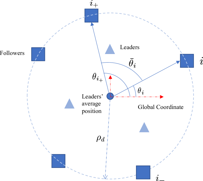
Figure 1: Configuration for the enclosing problem

The enclosing problem is demonstrated in Fig. 1, where the neighbor strategy taken in this work is the same as that in [12, 15] and thus is omitted. Specifically, the targets’ geometrical center is equally represented as the leader’s average position (LAP) in the following sections. Formally, it can be computed by:

𝒑¯t=1mi𝒱F𝒑itsuperscriptbold-¯𝒑𝑡1𝑚subscript𝑖subscript𝒱𝐹superscriptsubscript𝒑𝑖𝑡\boldsymbol{\bar{p}}^{t}=\frac{1}{m}\sum_{i\in\mathcal{V}_{F}}\boldsymbol{p}_{i}^{t} (4)

Given the LAP, we can define the relative position between follower i𝑖i and the LAP as:

Δ𝒑i=𝒑i𝒑¯𝒕=[Δpix,Δpiy]TΔsubscript𝒑𝑖subscript𝒑𝑖superscriptbold-¯𝒑𝒕superscriptΔsuperscriptsubscript𝑝𝑖𝑥Δsuperscriptsubscript𝑝𝑖𝑦𝑇\Delta\boldsymbol{p}_{i}=\boldsymbol{p}_{i}-\boldsymbol{\bar{p}^{t}}=[\Delta p_{i}^{x},\Delta p_{i}^{y}]^{T}

Then the relative angle between the follower i𝑖i and the LAP in the global frame is be denoted by

θi=atan2(ΔpiyΔpix).subscript𝜃𝑖𝑎𝑡𝑎𝑛2Δsuperscriptsubscript𝑝𝑖𝑦Δsuperscriptsubscript𝑝𝑖𝑥\theta_{i}=atan2(\frac{\Delta p_{i}^{y}}{\Delta p_{i}^{x}}).

As a result, the included angle from follower i𝑖i to its successor i+subscript𝑖i_{+} is defined by:

θ¯i=θi+θi+ςisubscript¯𝜃𝑖subscript𝜃subscript𝑖subscript𝜃𝑖subscript𝜍𝑖\bar{\theta}_{i}=\theta_{i_{+}}-\theta_{i}+\varsigma_{i} (5)

where

ςi={0,if θi+θi02π,if θi+θi<0\varsigma_{i}=\left\{\begin{aligned} 0,\text{if }\theta_{i_{+}}-\theta_{i}\geq 0\\ 2\pi,\text{if }\theta_{i_{+}}-\theta_{i}<0\end{aligned}\right. (6)

A predefined spacing pattern is encoded by ={wd,ρd,𝒂}subscript𝑤𝑑subscript𝜌𝑑𝒂\mathbb{P}=\{w_{d},\rho_{d},\boldsymbol{a}\}, which contains a set of desired included angles 𝒂=[a1,a2,,an]T𝒂superscriptsubscript𝑎1subscript𝑎2subscript𝑎𝑛𝑇\boldsymbol{a}=[a_{1},a_{2},\cdots,a_{n}]^{T}, a desired circling radius ρdsubscript𝜌𝑑\rho_{d} and a desired angular velocity wdsubscript𝑤𝑑w_{d} of followers when they finally rotate around the LAP. The pattern is said to be admissible if and only if i=1nai=2π,wd>0,formulae-sequencesuperscriptsubscript𝑖1𝑛subscript𝑎𝑖2𝜋subscript𝑤𝑑0\sum_{i=1}^{n}a_{i}=2\pi,w_{d}>0, and ρd>maxi𝒱L(𝒑it𝒑¯t2)subscript𝜌𝑑𝑚𝑎subscript𝑥𝑖subscript𝒱𝐿subscriptnormsuperscriptsubscript𝒑𝑖𝑡superscriptbold-¯𝒑𝑡2\rho_{d}>max_{i\in\mathcal{V}_{L}}(||\boldsymbol{p}_{i}^{t}-\boldsymbol{\bar{p}}^{t}||_{2}).

Problem 1: Given Assumptions 1 - 3 and the MAS composed of leaders in (2) and followers in (3), design a distributed controller for all followers such that they encircle the leaders (i.e. move along a common circle centered at the LAP) and the desired admissible spacing pattern \mathbb{P} is achieved in finite time.

IV Continuous finite-time estimator

Acquiring the exact LAP is the key for every follower to distributively accomplish the Problem 1. One intuitive method is to collect all leaders’ positions in each follower and then make the calculation directly according to its definition in (4). However, it is usually difficulty or impossible in reality due to various practical limitations. A more meaningful approach is to maintain an estimator for the LAP using only local information, for example, the observations to a subset of neighboring leaders and the exchanged messages from other neighboring followers. A well-studied estimator is designed as:

{𝒓i=𝚽i+𝒑~i,𝒑~i=nmj𝑵iT1|𝑵jF|𝒑jt.𝚽˙i=ksgnj𝑵i𝒓j𝒓i|𝒓j𝒓i|\left\{\begin{aligned} &\boldsymbol{{r}}_{i}=\boldsymbol{\Phi}_{i}+\boldsymbol{\tilde{p}}_{i},\qquad\boldsymbol{\tilde{p}}_{i}=\frac{n}{m}\sum_{j\in\boldsymbol{N}_{i}^{T}}\frac{1}{|\boldsymbol{N}_{j}^{F}|}\boldsymbol{p}_{j}^{t}.\\ &\boldsymbol{\dot{\Phi}}_{i}=k_{sgn}\sum_{j\in\boldsymbol{N}_{i}}\frac{\boldsymbol{r}_{j}-\boldsymbol{r}_{i}}{|\boldsymbol{r}_{j}-\boldsymbol{r}_{i}|}\end{aligned}\right. (7)

It has been investigated in [18, 19, 20, 21] that the output of this estimator 𝒓isubscript𝒓𝑖\boldsymbol{{r}}_{i} can exactly track the real LAP in finite time if Assumptions 1 - 3 hold and the estimator gain has ksgn>β(n1)subscript𝑘𝑠𝑔𝑛𝛽𝑛1k_{sgn}>\beta(n-1).

However, such estimator consists of the discontinuous term 𝒓j𝒓i|𝒓j𝒓i|subscript𝒓𝑗subscript𝒓𝑖subscript𝒓𝑗subscript𝒓𝑖\frac{\boldsymbol{r}_{j}-\boldsymbol{r}_{i}}{|\boldsymbol{r}_{j}-\boldsymbol{r}_{i}|}, which can result in dithering when either the estimator is getting converging or the adjacent estimators are similar. Regarding this problem, we propose a continuous estimator as following,

{𝒓i=𝚽i+𝒑~i,𝒑~i=nmj𝑵iT1|𝑵jF|𝒑j.𝚽˙i=kej𝑵iaij(𝒓j𝒓i)1α1\left\{\begin{aligned} &\boldsymbol{{r}}_{i}=\boldsymbol{\Phi}_{i}+\boldsymbol{\tilde{p}}_{i},\qquad\boldsymbol{\tilde{p}}_{i}=\frac{n}{m}\sum_{j\in\boldsymbol{N}_{i}^{T}}\frac{1}{|\boldsymbol{N}_{j}^{F}|}\boldsymbol{p}_{j}.\\ &\boldsymbol{\dot{\Phi}}_{i}=k_{e}\sum_{j\in\boldsymbol{N}_{i}}a_{ij}\left(\boldsymbol{r}_{j}-\boldsymbol{r}_{i}\right)^{\frac{1}{\alpha_{1}}}\end{aligned}\right. (8)

where α1=p1q1subscript𝛼1subscript𝑝1subscript𝑞1\alpha_{1}=\frac{p_{1}}{q_{1}}, and p1>q1>0subscript𝑝1subscript𝑞10p_{1}>q_{1}>0 are two positive odds. ke>0subscript𝑘𝑒0k_{e}>0 is the estimator gain. To show its effectiveness, we present the following theorem,

Theorem 3.

Given Assumptions 1 - 3, considering the system in (2) and (3), then if each follower in the MAS maintains an estimator (8), there exist a settling time T1subscript𝑇1T_{1} and a positive threshold ϵitalic-ϵ\epsilon, such that,

𝒓i𝒑¯t2ϵ,tT1formulae-sequencesubscriptnormsubscript𝒓𝑖superscriptbold-¯𝒑𝑡2italic-ϵfor-all𝑡subscript𝑇1||\boldsymbol{r}_{i}-\boldsymbol{\bar{p}}^{t}||_{2}\leq\epsilon,\forall t\geq T_{1} (9)

where the threshold can be adjusted by tuning the parameters in estimator.

Proof.

Considering a Lyapunouv candidate V1=12i,j=1n𝒓i𝒓j22=12i,j=1n(𝒓i𝒓j)T(𝒓i𝒓j)subscript𝑉112superscriptsubscript𝑖𝑗1𝑛superscriptsubscriptnormsubscript𝒓𝑖subscript𝒓𝑗2212superscriptsubscript𝑖𝑗1𝑛superscriptsubscript𝒓𝑖subscript𝒓𝑗𝑇subscript𝒓𝑖subscript𝒓𝑗V_{1}=\frac{1}{2}\sum_{i,j=1}^{n}||\boldsymbol{r}_{i}-\boldsymbol{r}_{j}||_{2}^{2}=\frac{1}{2}\sum_{i,j=1}^{n}\left(\boldsymbol{r}_{i}-\boldsymbol{r}_{j}\right)^{T}\left(\boldsymbol{r}_{i}-\boldsymbol{r}_{j}\right), its derivative has

V1˙=12i,j=1n[(𝒓˙i𝒓˙j)T(𝒓i𝒓j)+(𝒓i𝒓j)T(𝒓˙i𝒓˙j)]˙subscript𝑉112superscriptsubscript𝑖𝑗1𝑛delimited-[]superscriptsubscriptbold-˙𝒓𝑖subscriptbold-˙𝒓𝑗𝑇subscript𝒓𝑖subscript𝒓𝑗superscriptsubscript𝒓𝑖subscript𝒓𝑗𝑇subscriptbold-˙𝒓𝑖subscriptbold-˙𝒓𝑗\displaystyle\dot{V_{1}}=\frac{1}{2}\sum_{i,j=1}^{n}\left[(\boldsymbol{\dot{r}}_{i}-\boldsymbol{\dot{r}}_{j})^{T}\left(\boldsymbol{r}_{i}-\boldsymbol{r}_{j}\right)+\left(\boldsymbol{r}_{i}-\boldsymbol{r}_{j}\right)^{T}(\boldsymbol{\dot{r}}_{i}-\boldsymbol{\dot{r}}_{j})\right] (10)
=i,j=1n[(𝒓i𝒓j)T(𝚽˙i𝚽˙j)+(𝒓i𝒓j)T(𝒑~˙i𝒑~˙j)]absentsuperscriptsubscript𝑖𝑗1𝑛delimited-[]superscriptsubscript𝒓𝑖subscript𝒓𝑗𝑇subscriptbold-˙𝚽𝑖subscriptbold-˙𝚽𝑗superscriptsubscript𝒓𝑖subscript𝒓𝑗𝑇subscriptbold-˙bold-~𝒑𝑖subscriptbold-˙bold-~𝒑𝑗\displaystyle=\sum_{i,j=1}^{n}\left[\left(\boldsymbol{r}_{i}-\boldsymbol{r}_{j}\right)^{T}(\boldsymbol{\dot{\Phi}}_{i}-\boldsymbol{\dot{\Phi}}_{j})+\left(\boldsymbol{r}_{i}-\boldsymbol{r}_{j}\right)^{T}(\boldsymbol{\dot{\tilde{p}}}_{i}-\boldsymbol{\dot{\tilde{p}}}_{j})\right]

Substituting the estimator in (8) yields

V˙=i,j=1n[ke(𝒓i𝒓j)Ts1=1nais1(𝒓i𝒓s1)1α1\displaystyle\dot{V}=\sum_{i,j=1}^{n}\left[-k_{e}\left(\boldsymbol{r}_{i}-\boldsymbol{r}_{j}\right)^{T}\sum_{s_{1}=1}^{n}a_{is_{1}}\left(\boldsymbol{r}_{i}-\boldsymbol{r}_{s_{1}}\right)^{\frac{1}{\alpha_{1}}}\right. (11)
ke(𝒓i𝒓j)Ts2=1najs2(𝒓s2𝒓j)1α1+(𝒓i𝒓j)T(𝒑~˙i𝒑~˙j)]\displaystyle\left.-k_{e}\left(\boldsymbol{r}_{i}-\boldsymbol{r}_{j}\right)^{T}\sum_{s_{2}=1}^{n}a_{js_{2}}\left(\boldsymbol{r}_{s_{2}}-\boldsymbol{r}_{j}\right)^{\frac{1}{\alpha_{1}}}+\left(\boldsymbol{r}_{i}-\boldsymbol{r}_{j}\right)^{T}(\boldsymbol{\dot{\tilde{p}}}_{i}-\boldsymbol{\dot{\tilde{p}}}_{j})\right]
=ke2i,j=1n(s1=1nais1(𝒓i𝒓s1)1+α1α1+s2=1najs2(𝒓j𝒓s2)1+α1α1)+absentlimit-fromsubscript𝑘𝑒2superscriptsubscript𝑖𝑗1𝑛superscriptsubscriptsubscript𝑠11𝑛subscript𝑎𝑖subscript𝑠1superscriptsubscript𝒓𝑖subscript𝒓subscript𝑠11subscript𝛼1subscript𝛼1superscriptsubscriptsubscript𝑠21𝑛subscript𝑎𝑗subscript𝑠2superscriptsubscript𝒓𝑗subscript𝒓subscript𝑠21subscript𝛼1subscript𝛼1\displaystyle=-\frac{k_{e}}{2}\sum_{i,j=1}^{n}\left(\sum_{s_{1}=1}^{n}a_{is_{1}}(\boldsymbol{r}_{i}-\boldsymbol{r}_{s_{1}})^{\frac{1+\alpha_{1}}{\alpha_{1}}}+\sum_{s_{2}=1}^{n}a_{js_{2}}(\boldsymbol{r}_{j}-\boldsymbol{r}_{s_{2}})^{\frac{1+\alpha_{1}}{\alpha_{1}}}\right)+
kei=1n𝒓ij,s2=1najs2(𝒓j𝒓s2)1α1+kej=1n𝒓ji,s1=1nais1(𝒓i𝒓s1)1α1subscript𝑘𝑒superscriptsubscript𝑖1𝑛subscript𝒓𝑖superscriptsubscript𝑗subscript𝑠21𝑛subscript𝑎𝑗subscript𝑠2superscriptsubscript𝒓𝑗subscript𝒓subscript𝑠21subscript𝛼1subscript𝑘𝑒superscriptsubscript𝑗1𝑛subscript𝒓𝑗superscriptsubscript𝑖subscript𝑠11𝑛subscript𝑎𝑖subscript𝑠1superscriptsubscript𝒓𝑖subscript𝒓subscript𝑠11subscript𝛼1\displaystyle k_{e}\sum_{i=1}^{n}\boldsymbol{r}_{i}\sum_{j,s_{2}=1}^{n}a_{js_{2}}(\boldsymbol{r}_{j}-\boldsymbol{r}_{s_{2}})^{\frac{1}{\alpha_{1}}}+k_{e}\sum_{j=1}^{n}\boldsymbol{r}_{j}\sum_{i,s_{1}=1}^{n}a_{is_{1}}(\boldsymbol{r}_{i}-\boldsymbol{r}_{s_{1}})^{\frac{1}{\alpha_{1}}}
+i,j=1[(𝒓i𝒓j)T(𝒑~˙i𝒑~˙j)]subscript𝑖𝑗1delimited-[]superscriptsubscript𝒓𝑖subscript𝒓𝑗𝑇subscriptbold-˙bold-~𝒑𝑖subscriptbold-˙bold-~𝒑𝑗\displaystyle+\sum_{i,j=1}\left[\left(\boldsymbol{r}_{i}-\boldsymbol{r}_{j}\right)^{T}(\boldsymbol{\dot{\tilde{p}}}_{i}-\boldsymbol{\dot{\tilde{p}}}_{j})\right]

Recalling Lemma 2, it’s clear that

j=1ns2=1najs2(𝒓j𝒓s2)1α1=0superscriptsubscript𝑗1𝑛superscriptsubscriptsubscript𝑠21𝑛subscript𝑎𝑗subscript𝑠2superscriptsubscript𝒓𝑗subscript𝒓subscript𝑠21subscript𝛼10\sum_{j=1}^{n}\sum_{s_{2}=1}^{n}a_{js_{2}}(\boldsymbol{r}_{j}-\boldsymbol{r}_{s_{2}})^{\frac{1}{\alpha_{1}}}=0

and

i=1ns1=1nais1(𝒓i𝒓s1)1α1=0superscriptsubscript𝑖1𝑛superscriptsubscriptsubscript𝑠11𝑛subscript𝑎𝑖subscript𝑠1superscriptsubscript𝒓𝑖subscript𝒓subscript𝑠11subscript𝛼10\sum_{i=1}^{n}\sum_{s_{1}=1}^{n}a_{is_{1}}(\boldsymbol{r}_{i}-\boldsymbol{r}_{s_{1}})^{\frac{1}{\alpha_{1}}}=0

Therefore, the derivative can be rewritten into:

V1˙˙subscript𝑉1\displaystyle\dot{V_{1}} =nke2[i,s1=1nais1(𝒓i𝒓s1)1+α1α1+js2=1najs2(𝒓j𝒓s2)1+α1α1]absent𝑛subscript𝑘𝑒2delimited-[]superscriptsubscript𝑖subscript𝑠11𝑛subscript𝑎𝑖subscript𝑠1superscriptsubscript𝒓𝑖subscript𝒓subscript𝑠11subscript𝛼1subscript𝛼1superscriptsubscript𝑗subscript𝑠21𝑛subscript𝑎𝑗subscript𝑠2superscriptsubscript𝒓𝑗subscript𝒓subscript𝑠21subscript𝛼1subscript𝛼1\displaystyle=-\frac{nk_{e}}{2}\left[\sum_{i,s_{1}=1}^{n}a_{is_{1}}\left(\boldsymbol{r}_{i}-\boldsymbol{r}_{s_{1}}\right)^{\frac{1+\alpha_{1}}{\alpha_{1}}}+\sum_{js_{2}=1}^{n}a_{js_{2}}\left(\boldsymbol{r}_{j}-\boldsymbol{r}_{s_{2}}\right)^{\frac{1+\alpha_{1}}{\alpha_{1}}}\right] (12)
+i,j=1[(𝒓i𝒓j)T(𝒑~˙i𝒑~˙j)]subscript𝑖𝑗1delimited-[]superscriptsubscript𝒓𝑖subscript𝒓𝑗𝑇subscriptbold-˙bold-~𝒑𝑖subscriptbold-˙bold-~𝒑𝑗\displaystyle+\sum_{i,j=1}\left[\left(\boldsymbol{r}_{i}-\boldsymbol{r}_{j}\right)^{T}(\boldsymbol{\dot{\tilde{p}}}_{i}-\boldsymbol{\dot{\tilde{p}}}_{j})\right]
=nkei,s1=1nais1(𝒓i𝒓s1)1+1α1+i,j=1[(𝒓i𝒓j)T(𝒑~˙i𝒑~˙j)]absent𝑛subscript𝑘𝑒superscriptsubscript𝑖subscript𝑠11𝑛subscript𝑎𝑖subscript𝑠1superscriptsubscript𝒓𝑖subscript𝒓subscript𝑠111subscript𝛼1subscript𝑖𝑗1delimited-[]superscriptsubscript𝒓𝑖subscript𝒓𝑗𝑇subscriptbold-˙bold-~𝒑𝑖subscriptbold-˙bold-~𝒑𝑗\displaystyle=-nk_{e}\sum_{i,s_{1}=1}^{n}a_{is_{1}}\left(\boldsymbol{r}_{i}-\boldsymbol{r}_{s_{1}}\right)^{1+\frac{1}{\alpha_{1}}}+\sum_{i,j=1}\left[\left(\boldsymbol{r}_{i}-\boldsymbol{r}_{j}\right)^{T}(\boldsymbol{\dot{\tilde{p}}}_{i}-\boldsymbol{\dot{\tilde{p}}}_{j})\right]
nkei,s1=1nais1(𝒓i𝒓s1)1+1α1+2i,j=1[𝒑~˙i212𝒓i𝒓j2]absent𝑛subscript𝑘𝑒superscriptsubscript𝑖subscript𝑠11𝑛subscript𝑎𝑖subscript𝑠1superscriptsubscript𝒓𝑖subscript𝒓subscript𝑠111subscript𝛼12subscript𝑖𝑗1delimited-[]superscriptsubscriptnormsubscriptbold-˙bold-~𝒑𝑖212subscriptnormsubscript𝒓𝑖subscript𝒓𝑗2\displaystyle\leq-nk_{e}\sum_{i,s_{1}=1}^{n}a_{is_{1}}\left(\boldsymbol{r}_{i}-\boldsymbol{r}_{s_{1}}\right)^{1+\frac{1}{\alpha_{1}}}+2\sum_{i,j=1}\left[||\boldsymbol{\dot{\tilde{p}}}_{i}||_{2}^{\frac{1}{2}}||\boldsymbol{r}_{i}-\boldsymbol{r}_{j}||_{2}\right]

From the definition of 𝒑~isubscript~𝒑𝑖\tilde{\boldsymbol{p}}_{i} and Assumption 2, we know that |𝑵jF|1superscriptsubscript𝑵𝑗𝐹1|\boldsymbol{N}_{j}^{F}|\geq 1 and |𝑵iT|msuperscriptsubscript𝑵𝑖𝑇𝑚|\boldsymbol{N}_{i}^{T}|\leq m, which yields

𝒑~˙i2subscriptnormsubscriptbold-˙bold-~𝒑𝑖2\displaystyle||\boldsymbol{\dot{\tilde{p}}}_{i}||_{2} nmj𝑵iT1|𝑵jF|𝒑˙jt2absent𝑛𝑚subscript𝑗superscriptsubscript𝑵𝑖𝑇1superscriptsubscript𝑵𝑗𝐹subscriptnormsuperscriptsubscriptbold-˙𝒑𝑗𝑡2\displaystyle\leq\frac{n}{m}\sum_{j\in\boldsymbol{N}_{i}^{T}}\frac{1}{|\boldsymbol{N}_{j}^{F}|}||\boldsymbol{\dot{p}}_{j}^{t}||_{2}
nmaxj𝒱T𝒑˙jt2=nβabsent𝑛subscriptmax𝑗subscript𝒱𝑇subscriptnormsuperscriptsubscriptbold-˙𝒑𝑗𝑡2𝑛𝛽\displaystyle\leq n\text{max}_{j\in\mathcal{V}_{T}}||\boldsymbol{\dot{p}}_{j}^{t}||_{2}=n\beta

As a result,

V1˙˙subscript𝑉1\displaystyle\dot{V_{1}} nkei,s1=1nais1(𝒓i𝒓s1)1+1α1+2nβi,j=1𝒓i𝒓j2absent𝑛subscript𝑘𝑒superscriptsubscript𝑖subscript𝑠11𝑛subscript𝑎𝑖subscript𝑠1superscriptsubscript𝒓𝑖subscript𝒓subscript𝑠111subscript𝛼12𝑛𝛽subscript𝑖𝑗1subscriptnormsubscript𝒓𝑖subscript𝒓𝑗2\displaystyle\leq-nk_{e}\sum_{i,s_{1}=1}^{n}a_{is_{1}}\left(\boldsymbol{r}_{i}-\boldsymbol{r}_{s_{1}}\right)^{1+\frac{1}{\alpha_{1}}}+2n\beta\sum_{i,j=1}||\boldsymbol{r}_{i}-\boldsymbol{r}_{j}||_{2} (13)
nkeV1α1+12α1+2nβV112.absent𝑛subscript𝑘𝑒superscriptsubscript𝑉1subscript𝛼112subscript𝛼12𝑛𝛽superscriptsubscript𝑉112\displaystyle\leq-nk_{e}V_{1}^{\frac{\alpha_{1}+1}{2\alpha_{1}}}+2n\beta V_{1}^{\frac{1}{2}}.

If we let

nkeV1α1+12α1+2nβV112ηV112𝑛subscript𝑘𝑒superscriptsubscript𝑉1subscript𝛼112subscript𝛼12𝑛𝛽superscriptsubscript𝑉112𝜂superscriptsubscript𝑉112-nk_{e}V_{1}^{\frac{\alpha_{1}+1}{2\alpha_{1}}}+2n\beta V_{1}^{\frac{1}{2}}\leq-\eta V_{1}^{\frac{1}{2}}

i.e.

nkeV112α1𝑛subscript𝑘𝑒superscriptsubscript𝑉112subscript𝛼1\displaystyle-nk_{e}V_{1}^{\frac{1}{2\alpha_{1}}} +2nβη2𝑛𝛽𝜂\displaystyle+2n\beta\leq-\eta
V1subscript𝑉1\displaystyle V_{1} (η+2nβnke)2α1:=f(β,ke,α1)absentsuperscript𝜂2𝑛𝛽𝑛subscript𝑘𝑒2subscript𝛼1assign𝑓𝛽subscript𝑘𝑒subscript𝛼1\displaystyle\geq\left(\frac{\eta+2n\beta}{nk_{e}}\right)^{2\alpha_{1}}:=f(\beta,k_{e},\alpha_{1})

where η>0𝜂0\eta>0 is an arbitrary and f(β,ke,α1)𝑓𝛽subscript𝑘𝑒subscript𝛼1f(\beta,k_{e},\alpha_{1}) is a single-valued function with respect to the inputs, then

V˙1ηV112subscript˙𝑉1𝜂superscriptsubscript𝑉112\dot{V}_{1}\leq-\eta V_{1}^{\frac{1}{2}}

which means the Lyapunov function will converge to the set [0,f(β,ke,α1)]0𝑓𝛽subscript𝑘𝑒subscript𝛼1[0,f(\beta,k_{e},\alpha_{1})] in finite time

T12V112(0)f12(β,ke,α1)η.subscript𝑇12superscriptsubscript𝑉1120superscript𝑓12𝛽subscript𝑘𝑒subscript𝛼1𝜂T_{1}\leq 2\frac{V_{1}^{\frac{1}{2}}(0)-f^{\frac{1}{2}}(\beta,k_{e},\alpha_{1})}{\eta}.

and will stay within the set, i.e. V1(t)[0,f(β,ke,α1)],t>T1formulae-sequencesubscript𝑉1𝑡0𝑓𝛽subscript𝑘𝑒subscript𝛼1for-all𝑡subscript𝑇1V_{1}(t)\in[0,f(\beta,k_{e},\alpha_{1})],\forall t>T_{1}.

Since V1=i,j=1(𝒓i𝒓j)2subscript𝑉1subscript𝑖𝑗1superscriptsubscript𝒓𝑖subscript𝒓𝑗2V_{1}=\sum_{i,j=1}(\boldsymbol{r}_{i}-\boldsymbol{r}_{j})^{2}, for any two followers i,j𝑖𝑗i,j, the difference between their estimates has

𝒓i𝒓jV1f12(β,ke,α1)normsubscript𝒓𝑖subscript𝒓𝑗subscript𝑉1superscript𝑓12𝛽subscript𝑘𝑒subscript𝛼1||\boldsymbol{r}_{i}-\boldsymbol{r}_{j}||\leq\sqrt{V_{1}}\leq f^{\frac{1}{2}}(\beta,k_{e},\alpha_{1})

before the settling time T1subscript𝑇1T_{1}. In addition,

i=1n𝒓i(t)superscriptsubscript𝑖1𝑛subscript𝒓𝑖𝑡\displaystyle\sum_{i=1}^{n}\boldsymbol{r}_{i}(t) =ke0ti=1nj𝑵iaij(𝒓j𝒓i)1α1+i=1n𝒑~iabsentsubscript𝑘𝑒superscriptsubscript0𝑡superscriptsubscript𝑖1𝑛subscript𝑗subscript𝑵𝑖subscript𝑎𝑖𝑗superscriptsubscript𝒓𝑗subscript𝒓𝑖1subscript𝛼1superscriptsubscript𝑖1𝑛subscriptbold-~𝒑𝑖\displaystyle=k_{e}\int_{0}^{t}\sum_{i=1}^{n}\sum_{j\in\boldsymbol{N}_{i}}a_{ij}(\boldsymbol{r}_{j}-\boldsymbol{r}_{i})^{\frac{1}{\alpha_{1}}}+\sum_{i=1}^{n}\boldsymbol{\tilde{p}}_{i}

Since

i=1nj𝑵iaij(𝒓j𝒓i)1α1=0superscriptsubscript𝑖1𝑛subscript𝑗subscript𝑵𝑖subscript𝑎𝑖𝑗superscriptsubscript𝒓𝑗subscript𝒓𝑖1subscript𝛼10\sum_{i=1}^{n}\sum_{j\in\boldsymbol{N}_{i}}a_{ij}(\boldsymbol{r}_{j}-\boldsymbol{r}_{i})^{\frac{1}{\alpha_{1}}}=0

and

i=1n𝒑~i=i=1nnmj𝑵iT1|𝑵jF|𝒑jt=nmi=1m𝒑jt=n𝒑¯tsuperscriptsubscript𝑖1𝑛subscriptbold-~𝒑𝑖superscriptsubscript𝑖1𝑛𝑛𝑚subscript𝑗superscriptsubscript𝑵𝑖𝑇1superscriptsubscript𝑵𝑗𝐹superscriptsubscript𝒑𝑗𝑡𝑛𝑚superscriptsubscript𝑖1𝑚subscriptsuperscript𝒑𝑡𝑗𝑛superscriptbold-¯𝒑𝑡\sum_{i=1}^{n}\boldsymbol{\tilde{p}}_{i}=\sum_{i=1}^{n}\frac{n}{m}\sum_{j\in\boldsymbol{N}_{i}^{T}}\frac{1}{|\boldsymbol{N}_{j}^{F}|}\boldsymbol{p}_{j}^{t}=\frac{n}{m}\sum_{i=1}^{m}\boldsymbol{p}^{t}_{j}=n\boldsymbol{\bar{p}}^{t}

Therefore,

1ni=1n𝒓i=𝒑¯t.1𝑛superscriptsubscript𝑖1𝑛subscript𝒓𝑖subscriptbold-¯𝒑𝑡\frac{1}{n}\sum_{i=1}^{n}\boldsymbol{r}_{i}=\boldsymbol{\bar{p}}_{t}.

For any follower i𝒱F𝑖subscript𝒱𝐹i\in\mathcal{V}_{F}, the error between the real LAP and the output of the estimate in (8) is

𝒓i𝒑¯tnormsubscript𝒓𝑖superscriptbold-¯𝒑𝑡\displaystyle||\boldsymbol{r}_{i}-\boldsymbol{\bar{p}}^{t}|| =𝒓i1nj=1n𝒓jabsentnormsubscript𝒓𝑖1𝑛superscriptsubscript𝑗1𝑛subscript𝒓𝑗\displaystyle=||\boldsymbol{r}_{i}-\frac{1}{n}\sum_{j=1}^{n}\boldsymbol{r}_{j}||
=1nj=1n(𝒓i𝒓j)absentnorm1𝑛superscriptsubscript𝑗1𝑛subscript𝒓𝑖subscript𝒓𝑗\displaystyle=||\frac{1}{n}\sum_{j=1}^{n}(\boldsymbol{r}_{i}-\boldsymbol{r}_{j})||
1nj=1n(𝒓i𝒓j)absent1𝑛superscriptsubscript𝑗1𝑛normsubscript𝒓𝑖subscript𝒓𝑗\displaystyle\leq\frac{1}{n}\sum_{j=1}^{n}||(\boldsymbol{r}_{i}-\boldsymbol{r}_{j})||
f12(β,ke,α1)absentsuperscript𝑓12𝛽subscript𝑘𝑒subscript𝛼1\displaystyle\leq f^{\frac{1}{2}}(\beta,k_{e},\alpha_{1})

Let define ϵ=f12(β,ke,α1)italic-ϵsuperscript𝑓12𝛽subscript𝑘𝑒subscript𝛼1\epsilon=f^{\frac{1}{2}}(\beta,k_{e},\alpha_{1}), then this ends the proof of Theorem 3. ∎

Remark that Theorem 3 ensures that the proposed continuous estimator can achieve a bounded accuracy in finite time. The upper bound of accuracy can be adjusted by tuning the parameters ke,α1subscript𝑘𝑒subscript𝛼1k_{e},\alpha_{1} in the estimator. In practice, the preferred principles for determining kesubscript𝑘𝑒k_{e} and α1subscript𝛼1\alpha_{1} could be:

  1. 1.

    choose a large ke>0subscript𝑘𝑒0k_{e}>0 such that nke>η+2nβ𝑛subscript𝑘𝑒𝜂2𝑛𝛽nk_{e}>\eta+2n\beta.

  2. 2.

    given the desired accuracy ϵdsubscriptitalic-ϵ𝑑\epsilon_{d} and settling time T1,dsubscript𝑇1𝑑T_{1,d}, α1subscript𝛼1\alpha_{1} should satisfy:

    α1>lnϵdln(η+2nβ)ln(nke)subscript𝛼1subscriptitalic-ϵ𝑑𝜂2𝑛𝛽𝑛subscript𝑘𝑒\alpha_{1}>\frac{\ln\epsilon_{d}}{\ln(\eta+2n\beta)-\ln(nk_{e})}

    and

    α1>ln[V112(0)T1,dn(ke2β)2]ln(η+2nβ)ln(nke)subscript𝛼1superscriptsubscript𝑉1120subscript𝑇1𝑑𝑛subscript𝑘𝑒2𝛽2𝜂2𝑛𝛽𝑛subscript𝑘𝑒\alpha_{1}>\frac{\ln\left[V_{1}^{\frac{1}{2}}(0)-\frac{T_{1,d}n(k_{e}-2\beta)}{2}\right]}{\ln(\eta+2n\beta)-\ln(nk_{e})}

V Controller design

In this section, a controller is designed for Problem 1 to form the desired encircling formation. Firstly, we will show the property of finite-time convergence in Subsection V-A for the proposed controller without considering the estimated errors of the continuous estimators in (8). Then, the impact of estimated errors is analyzed in Subsection V-B.

V-A Finite-time enclosing controller

After obtaining the estimate of LAP in each follower, we can define the estimated relative distance error:

zi=ρiρdsubscript𝑧𝑖superscriptsubscript𝜌𝑖subscript𝜌𝑑z_{i}={\rho}_{i}^{{}^{\prime}}-\rho_{d} (14)

where ρi=Δ𝒑isuperscriptsubscript𝜌𝑖normΔsuperscriptsubscript𝒑𝑖{\rho}_{i}^{{}^{\prime}}=||\Delta\boldsymbol{p}_{i}^{{}^{\prime}}|| and Δ𝒑i=𝒑i𝒓iΔsuperscriptsubscript𝒑𝑖subscript𝒑𝑖subscript𝒓𝑖\Delta\boldsymbol{p}_{i}^{{}^{\prime}}=\boldsymbol{p}_{i}-\boldsymbol{r}_{i} are the relative position vector between the follower and the estimated LAP. Similar to the definition of θisubscript𝜃𝑖\theta_{i}, we can further define the estimated included angle using Δ𝒑iΔsuperscriptsubscript𝒑𝑖\Delta\boldsymbol{p}_{i}^{{}^{\prime}} as

θi=atan2(ΔpiyΔpix).superscriptsubscript𝜃𝑖𝑎𝑡𝑎𝑛2Δsuperscriptsubscript𝑝𝑖superscript𝑦Δsuperscriptsubscript𝑝𝑖superscript𝑥\theta_{i}^{{}^{\prime}}=atan2(\frac{\Delta p_{i}^{{}^{\prime}y}}{\Delta p_{i}^{{}^{\prime}x}}).

Then the error of estimated included angle is defined as:

δi=θ^1,θ^=θ¯iai,θ¯i=θi+θi+ςiformulae-sequencesubscript𝛿𝑖^𝜃1formulae-sequence^𝜃superscriptsubscript¯𝜃𝑖subscript𝑎𝑖superscriptsubscript¯𝜃𝑖superscriptsubscript𝜃limit-from𝑖superscriptsubscript𝜃𝑖subscript𝜍𝑖\delta_{i}=\hat{\theta}-1,\quad\hat{\theta}=\frac{\bar{\theta}_{i}^{{}^{\prime}}}{a_{i}},\quad\bar{\theta}_{i}^{{}^{\prime}}=\theta_{i+}^{{}^{\prime}}-\theta_{i}^{{}^{\prime}}+\varsigma_{i} (15)

It’s easy to verify that i=1naiδi=i=1nθ¯ii=1nai=2π2π=0superscriptsubscript𝑖1𝑛subscript𝑎𝑖subscript𝛿𝑖superscriptsubscript𝑖1𝑛subscript¯𝜃𝑖superscriptsubscript𝑖1𝑛subscript𝑎𝑖2𝜋2𝜋0\sum_{i=1}^{n}a_{i}\delta_{i}=\sum_{i=1}^{n}\bar{\theta}_{i}-\sum_{i=1}^{n}a_{i}=2\pi-2\pi=0, i.e. 𝒂T𝜹=0superscript𝒂𝑇𝜹0\boldsymbol{a}^{T}\boldsymbol{\delta}=0. The derivative of relative error is :

z˙isubscript˙𝑧𝑖\displaystyle\dot{z}_{i} =ρ˙iabsentsuperscriptsubscript˙𝜌𝑖\displaystyle=\dot{\rho}_{i}^{{}^{\prime}} (16)
=ddt(Δpix)2+(Δpiy)2absent𝑑𝑑𝑡superscriptΔsuperscriptsubscript𝑝𝑖superscript𝑥2superscriptΔsuperscriptsubscript𝑝𝑖superscript𝑦2\displaystyle=\frac{d}{dt}\sqrt{(\Delta p_{i}^{{}^{\prime}x})^{2}+(\Delta p_{i}^{{}^{\prime}y})^{2}}
=12ρiΔpix˙Δpix+Δpiy˙Δpiyabsent12superscriptsubscript𝜌𝑖˙Δsuperscriptsubscript𝑝𝑖superscript𝑥Δsuperscriptsubscript𝑝𝑖superscript𝑥˙Δsuperscriptsubscript𝑝𝑖superscript𝑦Δsuperscriptsubscript𝑝𝑖superscript𝑦\displaystyle=\frac{1}{2\rho_{i}^{{}^{\prime}}}\dot{\Delta p_{i}^{{}^{\prime}x}}\Delta p_{i}^{{}^{\prime}x}+\dot{\Delta p_{i}^{{}^{\prime}y}}\Delta p_{i}^{{}^{\prime}y}
=12ρiΔ𝒑˙iTΔ𝒑i=12ρiΔ𝒑iTΔ𝒑˙i=12𝝋iTΔ𝒑˙i\displaystyle=\frac{1}{2\rho_{i}^{{}^{\prime}}}\Delta\boldsymbol{\dot{p}}_{i}^{{}^{\prime}T}\Delta\boldsymbol{p}_{i}^{{}^{\prime}}=\frac{1}{2\rho_{i}^{{}^{\prime}}}\Delta\boldsymbol{{p}}_{i}^{{}^{\prime}T}\Delta\boldsymbol{\dot{p}}_{i}{{}^{\prime}}=\frac{1}{2}\boldsymbol{\varphi}_{i}^{{}^{\prime}T}\Delta\boldsymbol{\dot{p}}_{i}^{{}^{\prime}}

Regarding the included angle error, one has:

δ˙i=θ¯˙iai1,θ¯˙i=θ˙i+θ˙iformulae-sequencesubscript˙𝛿𝑖superscriptsubscript˙¯𝜃𝑖subscript𝑎𝑖1subscript˙¯𝜃𝑖superscriptsubscript˙𝜃subscript𝑖superscriptsubscript˙𝜃𝑖\dot{\delta}_{i}=\frac{\dot{\bar{\theta}}_{i}^{{}^{\prime}}}{a_{i}}-1,\quad\dot{\bar{\theta}}_{i}=\dot{\theta}_{i_{+}}^{{}^{\prime}}-\dot{\theta}_{i}^{{}^{\prime}} (17)

Further, we have:

θ˙isuperscriptsubscript˙𝜃𝑖\displaystyle\dot{\theta}_{i}^{{}^{\prime}} =11+(ΔpiyΔpiy)2ddt(ΔpiyΔpiy)absent11superscriptΔsuperscriptsubscript𝑝𝑖superscript𝑦Δsuperscriptsubscript𝑝𝑖superscript𝑦2𝑑𝑑𝑡Δsuperscriptsubscript𝑝𝑖superscript𝑦Δsuperscriptsubscript𝑝𝑖superscript𝑦\displaystyle=\frac{1}{1+(\frac{\Delta p_{i}^{{}^{\prime}y}}{\Delta p_{i}^{{}^{\prime}y}})^{2}}\frac{d}{dt}(\frac{\Delta p_{i}^{{}^{\prime}y}}{\Delta p_{i}^{{}^{\prime}y}}) (18)
=1ρi[Δpiy,Δpix][Δp˙ix,Δp˙iy]T1ρiabsent1superscriptsubscript𝜌𝑖Δsuperscriptsubscript𝑝𝑖superscript𝑦Δsuperscriptsubscript𝑝𝑖superscript𝑥superscriptΔsuperscriptsubscript˙𝑝𝑖superscript𝑥Δsuperscriptsubscript˙𝑝𝑖superscript𝑦𝑇1superscriptsubscript𝜌𝑖\displaystyle=\frac{1}{\rho_{i}^{{}^{\prime}}}[-\Delta p_{i}^{{}^{\prime}y},\Delta p_{i}^{{}^{\prime}x}][-\Delta\dot{p}_{i}^{{}^{\prime}x},\Delta\dot{p}_{i}^{{}^{\prime}y}]^{T}\frac{1}{\rho_{i}^{{}^{\prime}}}
=𝝋iTΔ𝒑˙i1ρiabsentsuperscriptsubscript𝝋perpendicular-to𝑖absentsuperscript𝑇Δsuperscriptsubscriptbold-˙𝒑𝑖1superscriptsubscript𝜌𝑖\displaystyle=\boldsymbol{\varphi}_{i\perp}^{{}^{\prime}T}\Delta\boldsymbol{\dot{p}}_{i}^{{}^{\prime}}\frac{1}{\rho_{i}^{{}^{\prime}}}

Let Δ𝒑=[Δ𝒑1,Δ𝒑2,,Δ𝒑n]T,𝒛=[z1,z2,,zn]T,𝜹=[δ1,δ2,,δn]Tformulae-sequenceΔsuperscript𝒑superscriptΔsuperscriptsubscript𝒑1Δsuperscriptsubscript𝒑2Δsuperscriptsubscript𝒑𝑛𝑇formulae-sequence𝒛superscriptsubscript𝑧1subscript𝑧2subscript𝑧𝑛𝑇𝜹superscriptsubscript𝛿1subscript𝛿2subscript𝛿𝑛𝑇\Delta\boldsymbol{p}^{{}^{\prime}}=[\Delta\boldsymbol{p}_{1}^{{}^{\prime}},\Delta\boldsymbol{p}_{2}^{{}^{\prime}},\cdots,\Delta\boldsymbol{p}_{n}^{{}^{\prime}}]^{T},\boldsymbol{z}=[z_{1},z_{2},\cdots,z_{n}]^{T},\boldsymbol{\delta}=[\delta_{1},\delta_{2},\cdots,\delta_{n}]^{T} be the compact vector of these variables respectively. Then we have

{𝒛˙=12diag([𝝋iT])Δ𝒑˙=12ϕΔ𝒑˙𝜹˙=𝑫1𝚲1𝑳θϕΔ𝒑˙\left\{\begin{aligned} \dot{\boldsymbol{z}}&=\frac{1}{2}diag([\boldsymbol{\varphi}_{i}^{{}^{\prime}T}])\Delta\boldsymbol{\dot{p}}^{{}^{\prime}}=\frac{1}{2}\boldsymbol{\phi}\Delta\boldsymbol{\dot{p}}^{{}^{\prime}}\\ \boldsymbol{\dot{\delta}}&=-\boldsymbol{D}^{-1}\boldsymbol{\Lambda}^{-1}\boldsymbol{L}_{\theta}\boldsymbol{\phi}_{\perp}\Delta\boldsymbol{\dot{p}}^{{}^{\prime}}\end{aligned}\right. (19)

where 𝑫=diag([ρi])n×n,𝑳θn×n=diag([lij])formulae-sequence𝑫𝑑𝑖𝑎𝑔delimited-[]superscriptsubscript𝜌𝑖superscript𝑛𝑛subscript𝑳𝜃superscript𝑛𝑛𝑑𝑖𝑎𝑔delimited-[]subscript𝑙𝑖𝑗\boldsymbol{D}=diag([\rho_{i}^{{}^{\prime}}])\in\mathbb{R}^{n\times n},\boldsymbol{L}_{\theta}\in\mathbb{R}^{n\times n}=diag([l_{ij}]) and Li,i=1,Li,i+=1formulae-sequencesubscript𝐿𝑖𝑖1subscript𝐿𝑖subscript𝑖1L_{i,i}=1,L_{i,i_{+}}=-1 and other elements are all zeros. The newly introduced matrices are defined as 𝚲=diag(𝒂)n×n,ϕ=diag([𝝋iT])n×2nformulae-sequence𝚲𝑑𝑖𝑎𝑔𝒂superscript𝑛𝑛bold-italic-ϕ𝑑𝑖𝑎𝑔delimited-[]superscriptsubscript𝝋𝑖superscript𝑇superscript𝑛2𝑛\boldsymbol{\Lambda}=diag(\boldsymbol{a})\in\mathbb{R}^{n\times n},\boldsymbol{\phi}=diag([\boldsymbol{\varphi}_{i}^{{}^{\prime}T}])\in\mathbb{R}^{n\times 2n}, and ϕ=diag([𝝋iT])n×2nsubscriptbold-italic-ϕperpendicular-to𝑑𝑖𝑎𝑔delimited-[]superscriptsubscript𝝋perpendicular-to𝑖absentsuperscript𝑇superscript𝑛2𝑛\boldsymbol{\phi}_{\perp}=diag([\boldsymbol{\varphi}_{i\perp}^{{}^{\prime}T}])\in\mathbb{R}^{n\times 2n}.

Then we design the following finite-time enclosing controller as:

{𝒖i=𝝋iTwz,i+𝝋i,Twδ,i+𝒓˙iwz,i=kzzi1α2wδ,i=kδδi1α3+wd\left\{\begin{aligned} &\boldsymbol{u}_{i}=\boldsymbol{\varphi}_{i}^{T}w_{z,i}+\boldsymbol{\varphi}_{i,\perp}^{T}w_{\delta,i}+\boldsymbol{\dot{r}}_{i}\\ &w_{z,i}=-k_{z}z^{\frac{1}{\alpha_{2}}}_{i}\\ &w_{\delta,i}=k_{\delta}\delta^{\frac{1}{\alpha_{3}}}_{i}+w_{d}\end{aligned}\right. (20)

It can be rewritten into a compact form as

{𝒖=ϕT𝒘z+ϕT𝒘δ+𝒓˙𝒘z=kz𝒛1α2𝒘δ=kδ𝜹1α3+𝒘d\left\{\begin{aligned} &\boldsymbol{u}=\boldsymbol{\phi}^{T}\boldsymbol{w}_{z}+\boldsymbol{\phi}_{\perp}^{T}\boldsymbol{w}_{\delta}+\boldsymbol{\dot{r}}\\ &\boldsymbol{w}_{z}=-k_{z}\boldsymbol{z}^{\frac{1}{\alpha_{2}}}\\ &\boldsymbol{w}_{\delta}=k_{\delta}\boldsymbol{\delta}^{\frac{1}{\alpha_{3}}}+\boldsymbol{w}_{d}\end{aligned}\right. (21)

where kz,kδsubscript𝑘𝑧subscript𝑘𝛿k_{z},k_{\delta} are two positive control gains, α2=p2q2,α3=p3q3formulae-sequencesubscript𝛼2subscript𝑝2subscript𝑞2subscript𝛼3subscript𝑝3subscript𝑞3\alpha_{2}=\frac{p_{2}}{q_{2}},\alpha_{3}=\frac{p_{3}}{q_{3}}, p2>q2>0,p3>q3>0formulae-sequencesubscript𝑝2subscript𝑞20subscript𝑝3subscript𝑞30p_{2}>q_{2}>0,p_{3}>q_{3}>0 are all positive odds, 𝒓˙bold-˙𝒓\boldsymbol{\dot{r}} is the derivative of the continuous estimator in (8), wdsubscript𝑤𝑑w_{d} is a constant indicating the desired rotating velocity for the enclosing formation.

Observing that Δ𝒑˙=𝒖𝒓˙Δsuperscriptbold-˙𝒑bold-′𝒖bold-˙𝒓\Delta\boldsymbol{\dot{p}^{{}^{\prime}}}=\boldsymbol{u}-\boldsymbol{\dot{r}} and 𝑳θ𝒘d=𝟎subscript𝑳𝜃subscript𝒘𝑑0\boldsymbol{L}_{\theta}\boldsymbol{w}_{d}=\boldsymbol{0}, we can substitute the controller in (21) into the error dynamics (19), which yields

{𝒛˙=kz2𝒛1α2𝜹˙=kδ𝑫1𝚲1𝑳θ𝜹1α3\left\{\begin{aligned} \dot{\boldsymbol{z}}&=-\frac{k_{z}}{2}\boldsymbol{z}^{\frac{1}{\alpha_{2}}}\\ \dot{\boldsymbol{\delta}}&=-k_{\delta}\boldsymbol{D}^{-1}\boldsymbol{\Lambda}^{-1}\boldsymbol{L}_{\theta}\boldsymbol{\delta}^{\frac{1}{\alpha_{3}}}\end{aligned}\right. (22)

Firstly, we show that the dynamic of the estimated included angle error 𝜹𝜹\boldsymbol{\delta} is globally asymptotically stable by the following lemma,

Lemma 3.

Let α3=p3q3subscript𝛼3subscript𝑝3subscript𝑞3\alpha_{3}=\frac{p_{3}}{q_{3}} and p3>q3>1subscript𝑝3subscript𝑞31p_{3}>q_{3}>1 be two positive odds, then the origin of

𝜹˙=kδ𝑫1𝚲1𝑳θ𝜹1α3˙𝜹subscript𝑘𝛿superscript𝑫1superscript𝚲1subscript𝑳𝜃superscript𝜹1subscript𝛼3\dot{\boldsymbol{\delta}}=-k_{\delta}\boldsymbol{D}^{-1}\boldsymbol{\Lambda}^{-1}\boldsymbol{L}_{\theta}\boldsymbol{\delta}^{\frac{1}{\alpha_{3}}}

is globally asymptotically stable.

Proof.

Considering the Lyapunouv candidate function V2=α3+1α3𝜹T𝜹1α3=α3+1α3i=1nδi1+1α3subscript𝑉2subscript𝛼31subscript𝛼3superscript𝜹𝑇superscript𝜹1subscript𝛼3subscript𝛼31subscript𝛼3superscriptsubscript𝑖1𝑛superscriptsubscript𝛿𝑖11subscript𝛼3V_{2}=\frac{\alpha_{3}+1}{\alpha_{3}}\boldsymbol{\delta}^{T}\boldsymbol{\delta}^{\frac{1}{\alpha_{3}}}=\frac{\alpha_{3}+1}{\alpha_{3}}\sum_{i=1}^{n}\delta_{i}^{1+\frac{1}{\alpha_{3}}}, its derivative has:

V˙2subscript˙𝑉2\displaystyle\dot{V}_{2} =i=1nδi1α3δ˙i=i=1nδi1α3kδaiρij=1naij(δi1α3δj1α3)absentsuperscriptsubscript𝑖1𝑛superscriptsubscript𝛿𝑖1subscript𝛼3subscript˙𝛿𝑖superscriptsubscript𝑖1𝑛superscriptsubscript𝛿𝑖1subscript𝛼3subscript𝑘𝛿subscript𝑎𝑖subscript𝜌𝑖superscriptsubscript𝑗1𝑛subscript𝑎𝑖𝑗superscriptsubscript𝛿𝑖1subscript𝛼3superscriptsubscript𝛿𝑗1subscript𝛼3\displaystyle=\sum_{i=1}^{n}\delta_{i}^{\frac{1}{\alpha_{3}}}\dot{\delta}_{i}=-\sum_{i=1}^{n}\delta_{i}^{\frac{1}{\alpha_{3}}}\frac{k_{\delta}}{a_{i}\rho_{i}}\sum_{j=1}^{n}a_{ij}(\delta_{i}^{\frac{1}{\alpha_{3}}}-\delta_{j}^{\frac{1}{\alpha_{3}}}) (23)
=12i=1nkδaiρij=1naij(δi1α3δj1α3)20absent12superscriptsubscript𝑖1𝑛subscript𝑘𝛿subscript𝑎𝑖subscript𝜌𝑖superscriptsubscript𝑗1𝑛subscript𝑎𝑖𝑗superscriptsuperscriptsubscript𝛿𝑖1subscript𝛼3superscriptsubscript𝛿𝑗1subscript𝛼320\displaystyle=-\frac{1}{2}\sum_{i=1}^{n}\frac{k_{\delta}}{a_{i}\rho_{i}}\sum_{j=1}^{n}a_{ij}(\delta_{i}^{\frac{1}{\alpha_{3}}}-\delta_{j}^{\frac{1}{\alpha_{3}}})^{2}\leq 0

The equality holds if and only if 𝜹=e𝟏𝜹𝑒1\boldsymbol{\delta}=e\boldsymbol{1}, where e𝑒e is a constant. Since the error vector has the relationship of 𝒂T𝜹=𝟎superscript𝒂𝑇𝜹0\boldsymbol{a}^{T}\boldsymbol{\delta}=\boldsymbol{0}, then the only solution for the equality is e=0𝑒0e=0. Thus, we have V˙20subscript˙𝑉20\dot{V}_{2}\leq 0 with V˙2=0subscript˙𝑉20\dot{V}_{2}=0 if and only if 𝜹=𝟎𝜹0\boldsymbol{\delta}=\boldsymbol{0}. Therefore, the origin is globally asymptotically stable. ∎
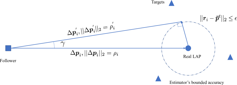
Refer to caption
Figure 2: Illustration for the impact of bounded accuracy

Next, the fact that dynamic of the estimated included angle error δ𝛿\vec{\delta} is a homogeneous system can be guaranteed by,

Lemma 4.

Define the vector field 𝐇(𝛅)=kδ𝐃1𝚲1𝐋θ𝛅1α3𝐇𝛅subscript𝑘𝛿superscript𝐃1superscript𝚲1subscript𝐋𝜃superscript𝛅1subscript𝛼3\boldsymbol{H}(\boldsymbol{\delta})=-k_{\delta}\boldsymbol{D}^{-1}\boldsymbol{\Lambda}^{-1}\boldsymbol{L}_{\theta}\boldsymbol{\delta}^{\frac{1}{\alpha_{3}}}, then it is homogeneous of degree 1α311subscript𝛼31\frac{1}{\alpha_{3}}-1 with respect to the standard dilation.

Proof.

Firstly, we show that δi1α3superscriptsubscript𝛿𝑖1subscript𝛼3\delta_{i}^{\frac{1}{\alpha_{3}}} is homogeneous of degree 1α31subscript𝛼3\frac{1}{\alpha_{3}} with respect to the standard dilation, i.e. for a λ>0𝜆0\lambda>0:

(λδi)1α3=λ1α3δi1α3superscript𝜆subscript𝛿𝑖1subscript𝛼3superscript𝜆1subscript𝛼3superscriptsubscript𝛿𝑖1subscript𝛼3(\lambda\delta_{i})^{\frac{1}{\alpha_{3}}}=\lambda^{\frac{1}{\alpha_{3}}}\delta_{i}^{\frac{1}{\alpha_{3}}}

Then, let’s denote the i𝑖i-th component of the vector field 𝑯(𝜹)𝑯𝜹\boldsymbol{H}(\boldsymbol{\delta}) as 𝑯i(𝜹)=1aiρij=1naij(δi1α3δj1α3)subscript𝑯𝑖𝜹1subscript𝑎𝑖subscript𝜌𝑖superscriptsubscript𝑗1𝑛subscript𝑎𝑖𝑗superscriptsubscript𝛿𝑖1subscript𝛼3superscriptsubscript𝛿𝑗1subscript𝛼3\boldsymbol{H}_{i}(\boldsymbol{\delta})=-\frac{1}{a_{i}\rho_{i}}\sum_{j=1}^{n}a_{ij}(\delta_{i}^{\frac{1}{\alpha_{3}}}-\delta_{j}^{\frac{1}{\alpha_{3}}}), whereby we can get:

𝑯i(λ𝜹)subscript𝑯𝑖𝜆𝜹\displaystyle\boldsymbol{H}_{i}(\lambda\boldsymbol{\delta}) =1aiρij=1naij[(λδi)1α3(λδj)1α3]absent1subscript𝑎𝑖subscript𝜌𝑖superscriptsubscript𝑗1𝑛subscript𝑎𝑖𝑗delimited-[]superscript𝜆subscript𝛿𝑖1subscript𝛼3superscript𝜆subscript𝛿𝑗1subscript𝛼3\displaystyle=-\frac{1}{a_{i}\rho_{i}}\sum_{j=1}^{n}a_{ij}\left[(\lambda\delta_{i})^{\frac{1}{\alpha_{3}}}-(\lambda\delta_{j})^{\frac{1}{\alpha_{3}}}\right]
=λ1α31aiρij=1naij(δi1α3δj1α3)absentsuperscript𝜆1subscript𝛼31subscript𝑎𝑖subscript𝜌𝑖superscriptsubscript𝑗1𝑛subscript𝑎𝑖𝑗superscriptsubscript𝛿𝑖1subscript𝛼3superscriptsubscript𝛿𝑗1subscript𝛼3\displaystyle=-\lambda^{\frac{1}{\alpha_{3}}}\frac{1}{a_{i}\rho_{i}}\sum_{j=1}^{n}a_{ij}\left(\delta_{i}^{\frac{1}{\alpha_{3}}}-\delta_{j}^{\frac{1}{\alpha_{3}}}\right)
=λ1α3𝑯i(𝜹)absentsuperscript𝜆1subscript𝛼3subscript𝑯𝑖𝜹\displaystyle=\lambda^{\frac{1}{\alpha_{3}}}\boldsymbol{H}_{i}(\boldsymbol{\delta})

Therefore, we say that the vector filed is homogeneous of degree 1α311subscript𝛼31\frac{1}{\alpha_{3}}-1 with respect to the standard dilation. ∎

Finally, we can conclude our main results of the finite-time controller as

Theorem 4.

Given Assumptions 1 - 3, consider the MAS composed of m𝑚m leaders in (2) and n𝑛n followers in (3), then if the each follower maintains an estimator in (8) and take the control input as (20), then the origin of the estimated error dynamics in (19) are finite-time stable, i.e. there exist settling time T2,T3subscript𝑇2subscript𝑇3T_{2},T_{3} such that:

{|ρiρd|=0,t>T2|θ¯iai|=0,t>T3\left\{\begin{aligned} |\rho_{i}^{{}^{\prime}}-\rho_{d}|=0,\forall t>T_{2}\\ |\bar{\theta}_{i}^{{}^{\prime}}-a_{i}|=0,\forall t>T_{3}\end{aligned}\right. (24)
Proof.

On the one hand, given the results from Lemma 3 - 4, we can immediately derive the property of finite time convergence for the estimated included angle errors 𝜹𝜹\boldsymbol{\delta} by recalling Theorem 2. Therefore, there exists a settling time T3subscript𝑇3T_{3} such that |θ¯iai|=0,t>T3formulae-sequencesuperscriptsubscript¯𝜃𝑖subscript𝑎𝑖0for-all𝑡subscript𝑇3|\bar{\theta}_{i}^{{}^{\prime}}-a_{i}|=0,\forall t>T_{3}.

On the other hand, regarding the estimated relative distance errors 𝒛𝒛\boldsymbol{z}, let consider the Lyapunouv function V2=12𝒛T𝒛=12i=1nzi2subscript𝑉212superscript𝒛𝑇𝒛12superscriptsubscript𝑖1𝑛superscriptsubscript𝑧𝑖2V_{2}=\frac{1}{2}\boldsymbol{z}^{T}\boldsymbol{z}=\frac{1}{2}\sum_{i=1}^{n}z_{i}^{2}. According to lemma 1, its derivative has:

V˙2subscript˙𝑉2\displaystyle\dot{V}_{2} =i=1nziz˙i=kzi=1nzi1+1α2absentsuperscriptsubscript𝑖1𝑛subscript𝑧𝑖subscript˙𝑧𝑖subscript𝑘𝑧superscriptsubscript𝑖1𝑛superscriptsubscript𝑧𝑖11subscript𝛼2\displaystyle=-\sum_{i=1}^{n}z_{i}\dot{z}_{i}=-k_{z}\sum_{i=1}^{n}z_{i}^{1+\frac{1}{\alpha_{2}}} (25)
=kzi=1n(zi2)α2+12α2kz(i=1nzi2)α2+12α2=kzV2α2+12α2absentsubscript𝑘𝑧superscriptsubscript𝑖1𝑛superscriptsuperscriptsubscript𝑧𝑖2subscript𝛼212subscript𝛼2subscript𝑘𝑧superscriptsuperscriptsubscript𝑖1𝑛superscriptsubscript𝑧𝑖2subscript𝛼212subscript𝛼2subscript𝑘𝑧superscriptsubscript𝑉2subscript𝛼212subscript𝛼2\displaystyle=-k_{z}\sum_{i=1}^{n}\left(z_{i}^{2}\right)^{\frac{\alpha_{2}+1}{2\alpha_{2}}}\leq-k_{z}\left(\sum_{i=1}^{n}z_{i}^{2}\right)^{\frac{\alpha_{2}+1}{2\alpha_{2}}}=-k_{z}V_{2}^{\frac{\alpha_{2}+1}{2\alpha_{2}}}

Therefore, the estimated relative distance errors 𝒛𝒛\boldsymbol{z} will converge to zeros in finite time T22α2kz(α21)V2(0)α212α2subscript𝑇22subscript𝛼2subscript𝑘𝑧subscript𝛼21subscript𝑉2superscript0subscript𝛼212subscript𝛼2T_{2}\leq\frac{2\alpha_{2}}{k_{z}(\alpha_{2}-1)}V_{2}(0)^{\frac{\alpha_{2}-1}{2\alpha_{2}}}.

This ends the proof of Theorem 4. ∎

Refer to caption
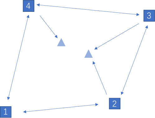
Figure 3: The network topology in the simulation case, where the rectangles and squares denote the followers and leaders, respectively. The arrows indicate connections within MAS. Note that the topology among followers is undirect and each leader is observed by at least one follower.

V-B Bounded error

The previous subsection shows that the proposed controller in (20) can achieve the desired spacing patter \mathbb{P} in finite time if the estimator can exactly track the real LAP in finite-time. However, the estimator designed in (8) can only guarantee a bounded accuracy in finite time. Therefore, the impact of the bounded accuracy on the controller is discussed in this subsection. Let define the real errors of both relative distance and the included angle as

{eρ,i=ρiρdeδ,i=θ¯iai1,\left\{\begin{aligned} e_{\rho,i}=\rho_{i}-\rho_{d}\\ e_{\delta,i}=\frac{\bar{\theta}_{i}}{a_{i}}-1,\end{aligned}\right. (26)
Refer to caption
(a) The error of estimated relative distance


Refer to caption
(b) The error of estimated included angle
Refer to caption
(c) The estimated error between real LAP and the output of estimator
Refer to caption
(d) The error of real relative distance


Refer to caption
(e) The error of real included angle
Refer to caption
(f) The control commands for all followers
Figure 5: The errors of both relative distances and included angles

Then we present our analysis as the following theorem,

Theorem 5.

Given Assumptions 1 - 3, consider the MAS composed of m𝑚m leaders in (2) and n𝑛n followers in (3), then if the each follower maintains an estimator in (8) and take the control input as (20), then there exist positive constants ϵρsubscriptitalic-ϵ𝜌\epsilon_{\rho} and ϵδsubscriptitalic-ϵ𝛿\epsilon_{\delta}, such that

{|eρ,i|<ϵρ,t>T1+T2+T3|eδ,i|<ϵδ,t>T1+T2+T3\left\{\begin{aligned} |e_{\rho,i}|<\epsilon_{\rho},\forall t>T_{1}+T_{2}+T_{3}\\ |e_{\delta,i}|<\epsilon_{\delta},\forall t>T_{1}+T_{2}+T_{3}\\ \end{aligned}\right. (27)
Proof.

Firstly, it’s obvious that

eρ,i=zi+ρiρisubscript𝑒𝜌𝑖subscript𝑧𝑖subscript𝜌𝑖superscriptsubscript𝜌𝑖e_{\rho,i}=z_{i}+\rho_{i}-\rho_{i}^{{}^{\prime}}

and

eδ,isubscript𝑒𝛿𝑖\displaystyle e_{\delta,i} =δi+θ¯iθ¯iaiabsentsubscript𝛿𝑖subscript¯𝜃𝑖subscriptsuperscript¯𝜃𝑖subscript𝑎𝑖\displaystyle=\delta_{i}+\frac{\bar{\theta}_{i}-\bar{\theta}^{{}^{\prime}}_{i}}{a_{i}}
=δi+(θi+θi+)(θiθi)aiabsentsubscript𝛿𝑖subscript𝜃limit-from𝑖superscriptsubscript𝜃limit-from𝑖subscript𝜃𝑖subscriptsuperscript𝜃𝑖subscript𝑎𝑖\displaystyle=\delta_{i}+\frac{\left(\theta_{i+}-\theta_{i+}^{{}^{\prime}}\right)-\left({\theta}_{i}-{\theta}^{{}^{\prime}}_{i}\right)}{a_{i}}
=δi+γi+γiaiabsentsubscript𝛿𝑖subscript𝛾limit-from𝑖subscript𝛾𝑖subscript𝑎𝑖\displaystyle=\delta_{i}+\frac{\gamma_{i+}-\gamma_{i}}{a_{i}}

where γi=θiθisubscript𝛾𝑖subscript𝜃𝑖superscriptsubscript𝜃𝑖\gamma_{i}=\theta_{i}-\theta_{i}^{{}^{\prime}} is the error between the real included angle and the estimated one as depicted in Fig. 2. Then, we can derive,

|eρ,i|<|ρiρi|<ϵ,t>T1+T2+T3formulae-sequencesubscript𝑒𝜌𝑖subscript𝜌𝑖superscriptsubscript𝜌𝑖italic-ϵfor-all𝑡subscript𝑇1subscript𝑇2subscript𝑇3|e_{\rho,i}|<|\rho_{i}-\rho_{i}^{{}^{\prime}}|<\epsilon,\forall t>T_{1}+T_{2}+T_{3} (28)

and

tan(γi)=ϵρdsubscript𝛾𝑖italic-ϵsubscript𝜌𝑑\displaystyle\tan(\gamma_{i})=\frac{\epsilon}{\rho_{d}} (29)
\displaystyle\Rightarrow |eδ,i|=|γi+γiai|2max|γi|ai<2arctanϵρdaisubscript𝑒𝛿𝑖subscript𝛾limit-from𝑖subscript𝛾𝑖subscript𝑎𝑖2subscript𝛾𝑖subscript𝑎𝑖2italic-ϵsubscript𝜌𝑑subscript𝑎𝑖\displaystyle|e_{\delta,i}|=|\frac{\gamma_{i+}-\gamma_{i}}{a_{i}}|\leq 2\frac{\max|\gamma_{i}|}{a_{i}}<\frac{2\arctan\frac{\epsilon}{\rho_{d}}}{a_{i}}

t>T1+T2+T3for-all𝑡subscript𝑇1subscript𝑇2subscript𝑇3\forall t>T_{1}+T_{2}+T_{3}. Therefore, we can define ϵρ=ϵsubscriptitalic-ϵ𝜌italic-ϵ\epsilon_{\rho}=\epsilon and ϵδ=2arctanϵρdaisubscriptitalic-ϵ𝛿2italic-ϵsubscript𝜌𝑑subscript𝑎𝑖\epsilon_{\delta}=\frac{2\arctan\frac{\epsilon}{\rho_{d}}}{a_{i}}.

This ends the proof of Theorem 5. ∎

VI Simulation

Refer to caption
Figure 6: Trajectories of all four followers and the real LAP over 200s

In the simulation, we consider the case with four followers and two leaders moving in 2-D plane. The network topology is demonstrated in Fig. 3, which meets the requirements of the Assumption. 1 and  2. The leaders are moving across the plane with bounded velocities that are unknown to all followers, which are respectively,

𝒗1=[10],𝒗2=[112sin(t10+π4)].formulae-sequencesubscript𝒗1matrix10subscript𝒗2matrix112𝑡10𝜋4\displaystyle\boldsymbol{v}_{1}=\begin{bmatrix}1\\ 0\end{bmatrix},\quad\boldsymbol{v}_{2}=\begin{bmatrix}1\\ \frac{1}{2}\sin(\frac{t}{10}+\frac{\pi}{4})\end{bmatrix}.

Therefore, the upper bound of target velocities is β=52𝛽52\beta=\frac{\sqrt{5}}{2}. The initial positions for both leaders and followers are listed in the Tab. I.

The desired spacing pattern \mathbb{P} is configured as follows. The desired relative distance between each agent and the real LAP is set to ρd=8subscript𝜌𝑑8\rho_{d}=8 m. The desired included angles between any pair of consecutive agents are fixed by 𝒂=[2π5,2π5,2π5,4π5]T𝒂superscript2𝜋52𝜋52𝜋54𝜋5𝑇\boldsymbol{a}=[\frac{2\pi}{5},\frac{2\pi}{5},\frac{2\pi}{5},\frac{4\pi}{5}]^{T}. The controller parameters are designed as in Tab. II. Through simple calculation, we derive that

{infη0(ϵ,ϵρ)=(2nβnke)2α10.099949infη0ϵδ=2arctanϵρdminai0.0199\left\{\begin{aligned} &\inf_{\eta\rightarrow 0}(\epsilon,\epsilon_{\rho})=\left(\frac{2n\beta}{nk_{e}}\right)^{2\alpha_{1}}\approx 0.099949\\ &\inf_{\eta\rightarrow 0}\epsilon_{\delta}=\frac{2\arctan\frac{\epsilon}{\rho_{d}}}{\min a_{i}}\approx 0.0199\end{aligned}\right.
TABLE I: Initial positions for the simulation case
Nodes Followers Leaders
F1subscript𝐹1F_{1} F1subscript𝐹1F_{1} F1subscript𝐹1F_{1} F1subscript𝐹1F_{1} L1subscript𝐿1L_{1} L2subscript𝐿2L_{2}
Pos(m) [10;20]1020[10;-20] [18;12]1812[18;12] [4;12]412[4;12] [2;16]216[-2;16] [0;0]00[0;0] [1;1]11[1;1]
TABLE II: Parameters for the designed controller
kesubscript𝑘𝑒k_{e} α1subscript𝛼1\alpha_{1} kzsubscript𝑘𝑧k_{z} α2subscript𝛼2\alpha_{2} kδsubscript𝑘𝛿k_{\delta} α3subscript𝛼3\alpha_{3}
6 7373\frac{7}{3} 2 333 2 333

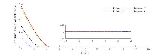
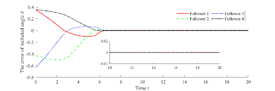
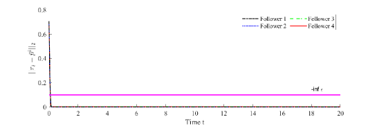
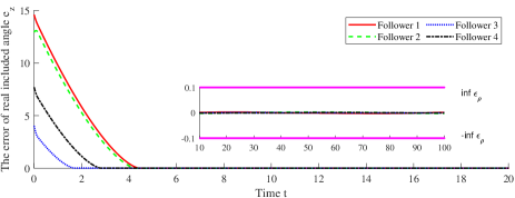
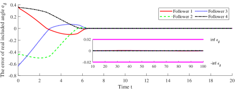
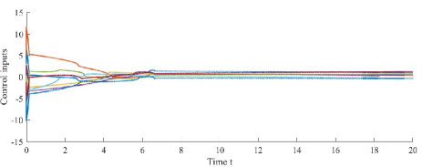
The simulation results are demonstrated from Figs. 5 - 6. Specifically, Fig. 5 shows the performance of the controller in (21) and estimator in (8), where Fig. 5(a) and Fig. 5(b) are the evolution of the estimated errors of both the relative distances zi,i𝒱Fsubscript𝑧𝑖for-all𝑖subscript𝒱𝐹z_{i},\forall i\in\mathcal{V}_{F} and included angles δi,i𝒱Fsubscript𝛿𝑖for-all𝑖subscript𝒱𝐹\delta_{i},\forall i\in\mathcal{V}_{F}. As proven by Theorem 4, they are exactly stabilized in finite-time. The real errors ez,isubscript𝑒𝑧𝑖e_{z,i} and eδ,isubscript𝑒𝛿𝑖e_{\delta,i} demonstrated in Fig 5(d) and Fig. 5(e), however, converge to their theoretical accuracy in finite time as shown in Theorem 5. Fig. 5(c) shows the error between the real LAP and the output of continuous estimators that are maintained by all followers. We can see that the errors of all four estimators quickly converge into the stable region [0,ϵ]0italic-ϵ[0,\epsilon], which validates the correctness of Theorem 3. Although these errors are not exactly zeros in finite time, they become quite smaller than the theoretical accuracy ϵitalic-ϵ\epsilon. Fig. 5(f) presents the control commands of all followers over the simulation, which validate that the designed controller and estimator don’t cause dithering during the enclosing process. Lastly, Fig. 6 gives the trajectories of all followers up to 200s. From Figs. 5 - 6, we can see that the desired spacing pattern is achieved in finite time and can be maintained within the theoretical accuracy.

VII Conclusion

The finite-time enclosing control problem using a multi-agent system for multiple moving targets is investigated in this paper. The proposed distributed estimator can track the geometrical center of multiple moving targets in finite time using only local information and the tracking accuracy is shown to be bounded and adjustable. Based on the output of this estimator, a pair of decentralized enclosing control laws are developed to achieve the desired spacing pattern in finite time. The steady errors of both the relative distance and included angle is bounded and can be adjusted by tuning the parameters in both estimator and controller. Future works may focus on reducing the tracking and controlling errors, extending the results to more general vehicles and so on.

References

  • [1] G. Beni, “From swarm intelligence to swarm robotics,” in International Workshop on Swarm Robotics.   Springer, 2004, pp. 1–9.
  • [2] D. Cushing and F. H. Jones, “Why do fish school?” Nature, vol. 218, no. 5145, pp. 918–920, 1968.
  • [3] F. Berlinger, M. Gauci, and R. Nagpal, “Implicit coordination for 3d underwater collective behaviors in a fish-inspired robot swarm,” Science Robotics, vol. 6, no. 50, 2021.
  • [4] M. Dorigo, G. Theraulaz, and V. Trianni, “Reflections on the future of swarm robotics,” Science Robotics, vol. 5, no. 49, 2020.
  • [5] H. Yamaguchi, “A cooperative hunting behavior by mobile-robot troops,” the International Journal of robotics Research, vol. 18, no. 9, pp. 931–940, 1999.
  • [6] C. Schumacher, “Ground moving target engagement by cooperative uavs,” in Proceedings of the 2005, American Control Conference, 2005.   IEEE, 2005, pp. 4502–4505.
  • [7] Y. Lan, G. Yan, and Z. Lin, “Distributed control of cooperative target enclosing based on reachability and invariance analysis,” Systems & Control Letters, vol. 59, no. 7, pp. 381–389, 2010.
  • [8] R. Zheng, Y. Liu, and D. Sun, “Enclosing a target by nonholonomic mobile robots with bearing-only measurements,” Automatica, vol. 53, pp. 400–407, 2015.
  • [9] C. Li, L. Chen, Y. Guo, and Y. Lyu, “Cooperative surrounding control with collision avoidance for networked lagrangian systems,” Journal of the Franklin Institute, vol. 355, no. 12, pp. 5182–5202, 2018.
  • [10] T.-H. Kim and T. Sugie, “Cooperative control for target-capturing task based on a cyclic pursuit strategy,” Automatica, vol. 43, no. 8, pp. 1426–1431, 2007.
  • [11] S. Hara, T.-H. Kim, and Y. Hori, “Distributed formation control for target-enclosing operations based on a cyclic pursuit strategy,” IFAC Proceedings Volumes, vol. 41, no. 2, pp. 6602–6607, 2008.
  • [12] J. Guo, G. Yan, and Z. Lin, “Local control strategy for moving-target-enclosing under dynamically changing network topology,” Systems & Control Letters, vol. 59, no. 10, pp. 654–661, 2010.
  • [13] B. Xu, H.-T. Zhang, H. Meng, B. Hu, D. Chen, and G. Chen, “Moving target surrounding control of linear multiagent systems with input saturation,” IEEE Transactions on Systems, Man, and Cybernetics: Systems, pp. 1–11, 2020.
  • [14] X. Peng, K. Guo, X. Li, and Z. Geng, “Cooperative moving-target enclosing control for multiple nonholonomic vehicles using feedback linearization approach,” IEEE Transactions on Systems, Man, and Cybernetics: Systems, vol. 51, no. 8, pp. 4929–4935, 2021.
  • [15] L. Dou, X. Yu, L. Liu, X. Wang, and G. Feng, “Moving-target enclosing control for mobile agents with collision avoidance,” IEEE Transactions on Control of Network Systems, pp. 1–1, 2021.
  • [16] F. Chen, W. Ren, and Y. Cao, “Surrounding control in cooperative agent networks,” Systems & Control Letters, vol. 59, no. 11, pp. 704–712, 2010.
  • [17] L. Zhang, Z. Zhang, Y. Qiao, and X. Wei, “Surrounding control in cooperative second-order agent networks,” in IECON 2017-43rd Annual Conference of the IEEE Industrial Electronics Society.   IEEE, 2017, pp. 5604–5609.
  • [18] Y. Shi, R. Li, and K. L. Teo, “Cooperative enclosing control for multiple moving targets by a group of agents,” International Journal of Control, vol. 88, no. 1, pp. 80–89, 2015.
  • [19] A. Sharghi, M. Baradarannia, and F. Hashemzadeh, “Finite-time-estimation-based surrounding control for a class of unknown nonlinear multi-agent systems,” Nonlinear Dynamics, vol. 96, no. 3, pp. 1795–1804, 2019.
  • [20] L. Zhang, Z. Li, and P. Gao, “Finite-time surrounding control of multi-agent systems with multiple targets,” in 2019 IEEE 8th Data Driven Control and Learning Systems Conference (DDCLS).   IEEE, 2019, pp. 231–236.
  • [21] D. Ma and Y. Sun, “Finite-time circle surrounding control for multi-agent systems,” International Journal of Control, Automation and Systems, vol. 15, no. 4, pp. 1536–1543, 2017.
  • [22] L. Wang and F. Xiao, “Finite-time consensus problems for networks of dynamic agents,” IEEE Transactions on Automatic Control, vol. 55, no. 4, pp. 950–955, 2010.
  • [23] S. P. Bhat and D. S. Bernstein, “Geometric homogeneity with applications to finite-time stability,” Mathematics of Control Signals & Systems, vol. 17, no. 2, pp. 101–127, 2005.