On a hybrid continuum-kinetic model for complex fluids

A. Chertock Department of Mathematics, North Carolina State University, USA; chertock@math.ncsu.edu    P. Degond Institut de Mathématiques de Toulouse; UMR5219; Université de Toulouse; CNRS; UPS; F-31062 Toulouse Cedex 9, France; pierre.degond@math.univ-toulouse.fr    G. Dimarco Department of Mathematics and Computer Science &\& Center for Modeling, Computing and Statistics of University of Ferrara, Italy; giacomo.dimarco@unife.it    M. Lukáčová-Medvid’ová Institute of Mathematics, University of Mainz, Germany; lukacova@uni-mainz.de    A. Ruhi Institute of Mathematics, University of Mainz, Germany; ankruh@gmail.com
Abstract

In the present work, we first introduce a general framework for modelling complex multiscale fluids and then focus on the derivation and analysis of a new hybrid continuum-kinetic model. In particular, we combine conservation of mass and momentum for an isentropic macroscopic model with a kinetic representation of the microscopic behavior. After introducing a small scale of interest, we compute the complex stress tensor by means of the Irving–Kirkwood formula. The latter requires an expansion of the kinetic distribution around an equilibrium state and a successive homogenization over the fast in time and small in space scale dynamics. For a new hybrid continuum-kinetic model the results of linear stability analysis indicate a conditional stability in the relevant low speed regimes and linear instability for high speed regimes for higher modes. Extensive numerical experiments confirm that the proposed multiscale model can reflect new phenomena of complex fluids not being present in standard Newtonian fluids. Consequently, the proposed general technique can be successfully used to derive new interesting systems combining the macro and micro structure of a given physical problem.

Keywords: multiscale simulations; hybrid method; kinetic equations; homogenization; scale separation; Newtonian and non-Newtonian flows; fluid dynamics; complex fluids

MSC: 76Nxx, 82C40, 76A05, 76M25

1 Introduction

Many important fluid flow problems are entirely multiscale: microscopic processes strongly influence macroscopic behavior of the fluid and need to be taken into account in order to accurately describe fluid dynamics. Typical examples are granular [33] and high-speed rarefied flows [6], the plastic deformation in materials [31], the viscoelastic [29] and biological type of fluids [37]. For this reason, in the last few decades, there has been a huge interest in both modeling and numerical simulations of problems associated with multilevel physical models, which are able to incorporate multiscale effects in different ways.

For the Newtonian fluids there have been many rigorous theoretical studies of hydrodynamic limits and the relationship between microscopic molecular dynamics and/or mesoscopic kinetic models of the Boltzmann type with macroscopic models such as the compressible Euler or Navier-Stokes equations, see, e.g., [2, 10, 22, 21, 28] and the references therein. On the other hand, for complex fluids theoretical understanding is certainly less developed, and more research is needed. More precisely, compared to standard fluids, the challenge associated with complex fluids lies in an accurate determination of rheological relations that are typically obtained from physical or computational experiments. Consequently, in many situations, e.g., soft matters or colloid-polymer mixtures, their full analytical description is not available.

In order to take small scale effects into account we can apply either mesoscopic kinetic models or directly microscopic models, such as molecular dynamics or dissipative particle dynamics, to reconstruct time evolution of macroscopic quantities. However, as is well known, an obvious drawback of meso- and microscopic descriptions, despite their higher accuracy, is sometimes prohibitively high computational costs, which limit their direct application in many practical situations. To overcome this disadvantage and make large-scale simulations possible the so-called hybrid multiscale methods have been developed in the literature. The latter combine the advantages of both descriptions: the accuracy of microscopic models to be able to consider complex rheological relationships with the efficiency of macroscopic models based on using classical conservation laws.

A prototype of hybrid multiscale methods is the heterogeneous multiscale method proposed by E, Enquist et al. [16, 14, 15, 17, 19, 34], see also [8, 38, 36, 39, 40] for its application for complex polymeric fluids. In this context let us also refer to triple-decker atomistic-mesoscopic-continuum method [20], the seamless multiscale methods [35, 18], the equation-free multiscale methods [25, 26] or the internal-flow multiscale method [4, 5]. In [27] a overview of multiscale flow simulations using particles is presented. For classical gas dynamics, similar ideas were employed, for instance, in [11, 9, 7, 32].

However, such general methods can have several disadvantages: the precise definition of the area in which the microscopic model should be applied is problem-dependent and needs to be specified. If the microscopic description is applied (almost) everywhere, the computational cost may become even larger than the cost required to numerically solve a micro- or mesoscale model. Clearly, bridging the large range of dynamically coupled scales is a fundamental challenge that was and still is a driving force in the development of new mathematical algorithms.

The goal of the present paper is to derive and analyse a new hybrid continuum-kinetic model for complex fluids. We start first by introducing a general methodological approach, which allows us to derive a class of new multiscale models. The basic idea is based on two simple ingredients. First, we assume that the problems we are studying have fast and slow scale dynamics. In addition, we assume a scale separation between the microscopic (fast) and macroscopic (slow) dynamics and thus, the phenomena may be imagined to act at different domain scales. Second, we assume that the effects of the fast scale dynamics on microscopic scale can be captured at the macroscopic level, at least approximately, by homogenization of the microscopic properties of the fluid over a finite size domain. In this work, we consider a prototype situation of isentropic flows governed by the conservation of mass and momentum at the continuum level. In order to model rheology of a complex fluid, the non-Newtonian stress tensor is obtained by an upscaling homogenizing procedure using the kinetic relaxation type equations. We will study properties of the derived hybrid multiscale model using a linear stability analysis and successively conduct several numerical experiments to illustrate the accuracy and efficiency of the proposed hybrid model.

The rest of the paper is organized in the following way. In Section 2, we derive the hybrid continuum-kinetic model including the non-Newtonian stress tensor. The latter is obtained by the Irving-Kirkwood formula which represents upscale microscopic effects. In Section 3, we perform a linear stability analysis which shows that for the regimes of interest, the low speed flows, the model is linearly stable. In Section 4, several numerical examples are conducted that demonstrate the validity of the proposed model for different prototype situations arising in complex flows. Finally, Section 5 is dedicated to the discussion of the obtained results and future developments.

2 The hybrid model approach

In this section, we first detail the general framework which will be used to derive a class of hybrid multiscale models. We then focus on the derivation and analysis of a prototype case, a hybrid continuum-kinetic model for complex fluids. This is realized by homogenization over a fixed size cell of the microscopic domains composed by the fluid molecules. The latter process leads to the Irving-Kirkwood formula for complex macroscopic stress tensor.

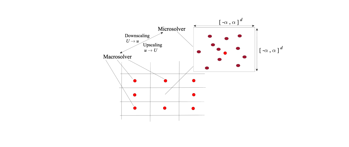
We start by considering the following general setting. We assume that a microscopic process used to describe time evolution of the state of the system of interest is known. For instance, molecular dynamics or kinetic mesoscopic equations are able to provide such information accurately enough. We also assume that we have at our disposal a macroscopic model in which a missing information will be provided by means of a microscopic model. These two models, micro/meso and macro, can be related through a reconstruction (upscaling) and a projection (downscaling) operator which permits to commute from one system to the other. The upscaling operator averages the micro properties of the fluid up to a coarser description, while the downscaling operator uses the coarser description to obtain the unknown variables at the microscopic level. A classical example of the above operators are downscaling/upscaling operators between kinetic and macroscopic description. In this case, the upscaling procedure is obtained by the integration of the distribution function multiplied by the so-called collision invariants over the velocity space while the downscaling operator is recovered from the knowledge of the macroscopic variable defining a so-called equilibrium distribution. In such a setting, our aim is to be able to give a description of the state of the system by working on a given macroscopic grid, defined a-priori, and through the use of a macroscopic model bringing some information from the microscopic/mesoscopic dynamics. Schematically, the proposed method works as depicted in Figure 2.1. We upscale the microsolver information, which is determined by time evolution of the unknown 𝒖𝒖\bm{u}, through a homogenization on a box of fixed size [α,α]dsuperscript𝛼𝛼𝑑[-\alpha,\alpha]^{d} with d𝑑d the spatial dimension and α𝛼\alpha the characteristic length of the microscopic variation. The size of the box depends on the problem under consideration. This micro information is successively used into the macroscopic solver, with unknown 𝑼𝑼\bm{U}, over the macroscopic grid to update the solution of the complex flow.

In what follows, we describe the details of such procedure in the case, where the macroscopic model is represented by the isentropic fluid equations for complex fluids while the microscopic model is the BGK kinetic equation [3]. From the depicted scenario, it is possible to imagine alternative types of combination of micro and macro dynamics which will be discussed in future investigations.
Refer to caption
Figure 2.1: Sketch of the hybrid multiscale approach.

2.1 A prototype case and derivation of the model

In this section, we consider a fluid which, by hypothesis, can be described at the macroscopic level by the compressible isentropic fluid equations. In this case, the system is governed by two equations describing the conservation of mass and momentum. This system reads

tρ+𝒙(ρ𝒖)=0,t(ρ𝒖)+𝒙(ρ𝒖𝒖)=𝒙𝕋,formulae-sequencesubscript𝑡𝜌subscript𝒙𝜌𝒖0subscript𝑡𝜌𝒖subscript𝒙tensor-product𝜌𝒖𝒖subscript𝒙𝕋\begin{split}&\partial_{t}\rho+\nabla_{\bm{x}}\cdot(\rho\bm{u})=0,\\ &\partial_{t}(\rho\bm{u})+\nabla_{\bm{x}}\cdot(\rho\bm{u}\otimes\bm{u})=\nabla_{\bm{x}}\cdot\mathbb{T},\end{split} (2.1)

where ρ𝜌\rho and 𝒖𝒖\bm{u} stand for the fluid density and velocity, respectively. The so-called Cauchy stress tensor 𝕋𝕋\mathbb{T} describes specific rheological fluid properties. All unknowns are functions of space 𝒙d𝒙superscript𝑑\bm{x}\in\mathbb{R}^{d} and time t>0𝑡0t>0. For inviscid fluids, 𝕋=p𝕀𝕋𝑝𝕀\mathbb{T}=-p\mathbb{I}, where 𝕀𝕀\mathbb{I} is the identity tensor. This expression leads to the Euler equations. Considering isentropic fluids, pressure p=p(ρ)𝑝𝑝𝜌p=p(\rho) is a given function of density ρ.𝜌\rho.

If viscous effects are taken into account, the Cauchy stress tensor reads

𝕋=p𝕀+𝕊,𝕋𝑝𝕀𝕊\mathbb{T}=-p\mathbb{I}+\mathbb{S},

where 𝕊𝕊\mathbb{S} stands for the viscous stress. For Newtonian fluids, the latter is given by the Newton rheological rule (NRR)

𝕊=μ(𝒙𝒖+𝒙𝒖T2d𝒙𝒖𝕀)+λ𝒙𝒖𝕀,𝕊𝜇subscript𝒙𝒖subscript𝒙superscript𝒖𝑇2𝑑subscript𝒙𝒖𝕀𝜆subscript𝒙𝒖𝕀\mathbb{S}=\mu\left(\nabla_{\bm{x}}\bm{u}+\nabla_{\bm{x}}\bm{u}^{T}-\frac{2}{d}\nabla_{\bm{x}}\cdot\bm{u}\mathbb{I}\right)+\lambda\nabla_{\bm{x}}\cdot\bm{u}\mathbb{I},

with μ>0𝜇0\mu>0 and λ0𝜆0\lambda\geq 0 being the constant shear and bulk viscosity coefficients, respectively. This relation leads to the compressible Navier-Stokes equations. In complex fluids, however, the rheological relation for the Cauchy stress tensor is more general and typically obtained by computational or physical experiments. Here, we propose instead that the Cauchy stress tensor takes into account microscopic effects in a homogenized way. This new model is derived from considering the kinetic equations underpinning fluid models of the type (2.1) as a microscopic model.

More specifically, we make the hypothesis that the so-called BGK (Bhatnagar-Gross-Krook) equation is a suitable microscopic model which can be upscaled to yield a missing information on a complex Cauchy stress tensor at the macroscopic level. The considered BGK equation reads [3]

tf+𝒗𝒙f=Q(f),subscript𝑡𝑓𝒗subscript𝒙𝑓𝑄𝑓\partial_{t}f+\bm{v}\cdot\nabla_{\bm{x}}f=Q(f), (2.2)

where f𝑓f is the probability density function of fluid molecules at position 𝒙𝒙\bm{x} having velocity 𝒗d𝒗superscript𝑑\bm{v}\in\mathbb{R}^{d} at time t𝑡t and Q(f)𝑄𝑓Q(f) is a collision operator (modelling the molecular interactions) to be described later on. This hypothesis can be relaxed giving rise to similar models with, however, different coefficients.

We assume now as depicted in Figure 2.1 that f𝑓f has slow variations at the domain scale D𝐷D and fast variations at scale αDmuch-less-than𝛼𝐷\alpha\ll D. Given that hypothesis, we consequently set f=f~(𝒙,𝒙α,𝒗,t)𝑓~𝑓𝒙𝒙𝛼𝒗𝑡f=\tilde{f}(\bm{x},\frac{\bm{x}}{\alpha},\bm{v},t) where f~(𝒙,𝒚,𝒗,t)~𝑓𝒙𝒚𝒗𝑡\tilde{f}(\bm{x},\bm{y},\bm{v},t) is 2-periodic with respect to 𝒚𝒚\bm{y}, with unit cell [1,1]dsuperscript11𝑑[-1,1]^{d}. We also suppose that the collision operator has magnitude 1/α1𝛼1/\alpha, i.e. that the microscopic spatial effect are balanced by the collision dynamics among molecules. Substituting this representation into (2.2), yields the following microscopic model

tf~+𝒗𝒙f~+1α𝒗𝒚f~=1αQ(f~).subscript𝑡~𝑓𝒗subscript𝒙~𝑓1𝛼𝒗subscript𝒚~𝑓1𝛼𝑄~𝑓\partial_{t}\tilde{f}+\bm{v}\cdot\nabla_{\bm{x}}\tilde{f}+\frac{1}{\alpha}\bm{v}\cdot\nabla_{\bm{y}}\tilde{f}=\frac{1}{\alpha}Q(\tilde{f}). (2.3)

Now, we introduce two new functions, one for the density ρ~=ρ~(𝒙,𝒚,t)~𝜌~𝜌𝒙𝒚𝑡\tilde{\rho}=\tilde{\rho}(\bm{x},\bm{y},t) and one for the vector velocity 𝒖~=𝒖~(𝒙,𝒚,t)~𝒖~𝒖𝒙𝒚𝑡\tilde{\bm{u}}=\tilde{\bm{u}}(\bm{x},\bm{y},t) to be precisely defined later on. Q(f~)𝑄~𝑓Q(\tilde{f}) is the BGK operator, i.e. a relaxation operator towards a given Maxwellian distribution M(ρ~,𝒖~)subscript𝑀~𝜌~𝒖M_{(\tilde{\rho},\tilde{\bm{u}})} of parameter ρ~~𝜌\tilde{\rho} and 𝒖~~𝒖\tilde{\bm{u}}. We observe at this stage that the way in which ρ~~𝜌\tilde{\rho} and 𝒖~~𝒖\tilde{\bm{u}} will be defined will permit to close the resulting system of macroscopic equations. Denoting by T𝑇T the (constant) temperature and R𝑅R the universal gas constant, M(ρ~,𝒖~)subscript𝑀~𝜌~𝒖M_{(\tilde{\rho},\tilde{\bm{u}})} is given by

M(ρ~,𝒖~)(𝒗)=ρ~(2πRT)d/2exp(|𝒗𝒖~|22RT),subscript𝑀~𝜌~𝒖𝒗~𝜌superscript2𝜋𝑅𝑇𝑑2superscript𝒗~𝒖22𝑅𝑇M_{(\tilde{\rho},\tilde{\bm{u}})}(\bm{v})=\frac{\tilde{\rho}}{(2\pi RT)^{d/2}}\exp{\left(-\frac{|\bm{v}-\tilde{\bm{u}}|^{2}}{2RT}\right)}, (2.4)

and the BGK operator is given by

Q(f~)=1τ~(f~M(ρ~,𝒖~)),𝑄~𝑓1~𝜏~𝑓subscript𝑀~𝜌~𝒖Q(\tilde{f})=-\frac{1}{\tilde{\tau}}(\tilde{f}-M_{(\tilde{\rho},\tilde{\bm{u}})}), (2.5)

where τ~~𝜏\tilde{\tau} is a relaxation time. Finally, (2.3) takes the form

α(tf~+𝒗𝒙f~)+𝒗𝒚f~=1τ~(f~M(ρ~,𝒖~)).𝛼subscript𝑡~𝑓𝒗subscript𝒙~𝑓𝒗subscript𝒚~𝑓1~𝜏~𝑓subscript𝑀~𝜌~𝒖\alpha\big{(}\partial_{t}\tilde{f}+\bm{v}\cdot\nabla_{\bm{x}}\tilde{f}\big{)}+\bm{v}\cdot\nabla_{\bm{y}}\tilde{f}=-\frac{1}{\tilde{\tau}}(\tilde{f}-M_{(\tilde{\rho},\tilde{\bm{u}})}). (2.6)

The microscopic model (2.6) can be used to provide a missing detailed information for the macroscopic model (2.1). To this end, the Cauchy stress tensor 𝕋𝕋\mathbb{T} can be reconstructed from f~~𝑓\tilde{f} by an upscaling homogenization procedure through the Irving-Kirkwood (or Kramer) formula [23]:

𝕋(𝒙,t)=12d[1,1]dd(𝒗𝒖~(𝒙,𝒚,t))(𝒗𝒖~(𝒙,𝒚,t))f~(𝒙,𝒚,𝒗,t)𝑑𝒗𝑑𝒚𝕋𝒙𝑡1superscript2𝑑subscriptsuperscript11𝑑subscriptsuperscript𝑑tensor-product𝒗~𝒖𝒙𝒚𝑡𝒗~𝒖𝒙𝒚𝑡~𝑓𝒙𝒚𝒗𝑡differential-d𝒗differential-d𝒚\mathbb{T}(\bm{x},t)=-\frac{1}{2^{d}}\int\displaylimits_{\left[-1,1\right]^{d}}\int_{\mathbb{R}^{d}}(\bm{v}-\tilde{\bm{u}}(\bm{x},\bm{y},t))\otimes(\bm{v}-\tilde{\bm{u}}(\bm{x},\bm{y},t))\tilde{f}(\bm{x},\bm{y},\bm{v},t)d\bm{v}d\bm{y} (2.7)

with f~~𝑓\tilde{f} being the solution of (2.6). In other words, we measure the microscopic effects by homogenization of the kinetic model over the microscopic box of size [α,α]dsuperscript𝛼𝛼𝑑[-\alpha,\alpha]^{d}. Problem (2.6) can be viewed as a cell problem for 𝒚𝒚\bm{y} in the unit cell [1,1]dsuperscript11𝑑\left[-1,1\right]^{d} and 𝒗d𝒗superscript𝑑\bm{v}\in{\mathbb{R}}^{d}. The size of this box is left as a free parameter, which may depend on the system under consideration. An interesting setting, which will be numerically explored in Section 4, consists of considering the size of the box into relation with the macroscopic description of the flow at the numerical level. This can be done, for instance, by fixing a ratio between the box where the microscopic effects are measured and the size of the mesh employed at the macroscopic level.

In order to have a well posed problem, we finally supplement (2.6) with the periodic boundary conditions for the probability density function:

f~(𝒙,𝒚+𝒏,𝒗,t)=f~(𝒙,𝒚,𝒗,t),𝒏(2)d.formulae-sequence~𝑓𝒙𝒚𝒏𝒗𝑡~𝑓𝒙𝒚𝒗𝑡for-all𝒏superscript2𝑑\tilde{f}(\bm{x},\bm{y}+\bm{n},\bm{v},t)=\tilde{f}(\bm{x},\bm{y},\bm{v},t),\quad\forall\bm{n}\in(2\mathbb{Z})^{d}.

Our aim now is to find an approximate solution of the cell problem by means of the Chapman-Enskog expansion [6] for small relaxation times τ~~𝜏\tilde{\tau}. This will allow us to upscale the microscopic effects at the macroscopic level without resorting to the numerical resolution of the microscopic model which would lead to an expensive computation. This step is performed in the next section.

2.2 Chapman-Enskog expansion for the prototype hybrid model

In this part, we present a perturbation analysis of the distribution function f~~𝑓\tilde{f} over the box [1,1]d.superscript11𝑑[-1,1]^{d}. We assume in the rest of the paper that τ~=O(ε),~𝜏𝑂𝜀\tilde{\tau}=O(\varepsilon), where ε1much-less-than𝜀1\varepsilon\ll 1 is the Knudsen number, i.e. the ratio of the relaxation parameter τ~~𝜏\tilde{\tau} to a characteristic hydrodynamic temporal scale. The latter represents the macroscopic scale of interest in our analysis. More precisely, we write τ~=ετ^~𝜏𝜀^𝜏\tilde{\tau}=\varepsilon\hat{\tau}, where τ^=O(1)^𝜏𝑂1\hat{\tau}=O(1) when ε0𝜀0\varepsilon\rightarrow 0 in the following. We proceed by introducing the Chapman-Enskog expansion [6] that will be truncated at the first-order terms

f~ε=f~(0)+εf~(1)+𝒪(ε2),superscript~𝑓𝜀superscript~𝑓0𝜀superscript~𝑓1𝒪superscript𝜀2\tilde{f}^{\varepsilon}=\tilde{f}^{(0)}+\varepsilon\tilde{f}^{(1)}+{\mathcal{O}}(\varepsilon^{2}), (2.8)

where f~εsuperscript~𝑓𝜀\tilde{f}^{\varepsilon} is the solution of (2.6) when τ~~𝜏\tilde{\tau} is replaced by ετ^𝜀^𝜏\varepsilon\hat{\tau}. The so-called cell problem (2.3) is then rewritten, using the Einstein summation convention under the above scaling as

(α(tf~ε+vixif~ε)+viyif~ε)(𝒙,𝒚,𝒗,t)=1ετ^[f~ε(𝒙,𝒚,𝒗,t)M(ρ~ε(𝒙,𝒚,t),𝒖~ε(𝒙,𝒚,t))(𝒗)].𝛼subscript𝑡superscript~𝑓𝜀subscript𝑣𝑖subscriptsubscript𝑥𝑖superscript~𝑓𝜀subscript𝑣𝑖subscriptsubscript𝑦𝑖superscript~𝑓𝜀𝒙𝒚𝒗𝑡1𝜀^𝜏delimited-[]superscript~𝑓𝜀𝒙𝒚𝒗𝑡subscript𝑀superscript~𝜌𝜀𝒙𝒚𝑡superscript~𝒖𝜀𝒙𝒚𝑡𝒗\Big{(}\alpha\big{(}\partial_{t}\tilde{f}^{\varepsilon}+v_{i}\partial_{x_{i}}\tilde{f}^{\varepsilon}\big{)}+v_{i}\partial_{y_{i}}\tilde{f}^{\varepsilon}\Big{)}(\bm{x},\bm{y},\bm{v},t)=-\frac{1}{\varepsilon\hat{\tau}}\Big{[}\tilde{f}^{\varepsilon}(\bm{x},\bm{y},\bm{v},t)-M_{(\tilde{\rho}^{\varepsilon}(\bm{x},\bm{y},t),\tilde{\bm{u}}^{\varepsilon}(\bm{x},\bm{y},t))}(\bm{v})\Big{]}. (2.9)

Substituting (2.8) into (2.9) and equating the same powers of ε𝜀\varepsilon yields

f~(0)=M(ρ~,𝒖~),f~(1)=τ^(α(tf~(0)+vixif~(0))+viyif~(0)).formulae-sequencesuperscript~𝑓0subscript𝑀~𝜌~𝒖superscript~𝑓1^𝜏𝛼subscript𝑡superscript~𝑓0subscript𝑣𝑖subscriptsubscript𝑥𝑖superscript~𝑓0subscript𝑣𝑖subscriptsubscript𝑦𝑖superscript~𝑓0\tilde{f}^{(0)}=M_{(\tilde{\rho},\tilde{\bm{u}})},\quad\tilde{f}^{(1)}=-\hat{\tau}\Big{(}\alpha\big{(}\partial_{t}\tilde{f}^{(0)}+v_{i}\partial_{x_{i}}\tilde{f}^{(0)}\big{)}+v_{i}\partial_{y_{i}}\tilde{f}^{(0)}\Big{)}.

We proceed now, using the first order expansion (2.9), to the computation of the Cauchy stress tensor appearing in equation (2.1) in the above described setting. To this end, we denote

𝒯ijsubscript𝒯𝑖𝑗\displaystyle\mathcal{T}_{ij} =\displaystyle= d(vju~j)(viu~i)f~(0)𝑑𝒗+εd(vju~j)(viu~i)f~(1)𝑑𝒗+𝒪(ε2)subscriptsuperscript𝑑subscript𝑣𝑗subscript~𝑢𝑗subscript𝑣𝑖subscript~𝑢𝑖superscript~𝑓0differential-d𝒗𝜀subscriptsuperscript𝑑subscript𝑣𝑗subscript~𝑢𝑗subscript𝑣𝑖subscript~𝑢𝑖superscript~𝑓1differential-d𝒗𝒪superscript𝜀2\displaystyle\int_{\mathbb{R}^{d}}(v_{j}-\tilde{u}_{j})(v_{i}-\tilde{u}_{i})\tilde{f}^{(0)}d\bm{v}+\varepsilon\int_{\mathbb{R}^{d}}(v_{j}-\tilde{u}_{j})(v_{i}-\tilde{u}_{i})\tilde{f}^{(1)}d\bm{v}+{\mathcal{O}}(\varepsilon^{2})
=:absent:\displaystyle=: 𝒯ij(0)+𝒯ij(1)+𝒪(ε2),superscriptsubscript𝒯𝑖𝑗0superscriptsubscript𝒯𝑖𝑗1𝒪superscript𝜀2\displaystyle\mathcal{T}_{ij}^{(0)}+\mathcal{T}_{ij}^{(1)}+{\mathcal{O}}(\varepsilon^{2}),

the contribution to the stress tensor coming from the Chapmann-Enskog expansion and we consider in the following computations each term separately.

First, using the equation of state for perfect gases p~=RTρ~~𝑝𝑅𝑇~𝜌\tilde{p}=RT\tilde{\rho}, we obtain that the leading term in (2.2) can be written as

𝒯ij(0)subscriptsuperscript𝒯0𝑖𝑗\displaystyle\mathcal{T}^{(0)}_{ij} =d(vju~j)(viu~i)f~(0)𝑑𝒗absentsubscriptsuperscript𝑑subscript𝑣𝑗subscript~𝑢𝑗subscript𝑣𝑖subscript~𝑢𝑖superscript~𝑓0differential-d𝒗\displaystyle=\int_{\mathbb{R}^{d}}(v_{j}-\tilde{u}_{j})(v_{i}-\tilde{u}_{i})\tilde{f}^{(0)}d\bm{v} (2.11a)
=d(vju~j)(viu~i)ρ~(2πRT)d/2exp(|𝒗𝒖~|22RT)𝑑𝒗=ρ~RTδij=p~δijabsentsubscriptsuperscript𝑑subscript𝑣𝑗subscript~𝑢𝑗subscript𝑣𝑖subscript~𝑢𝑖~𝜌superscript2𝜋𝑅𝑇𝑑2superscript𝒗~𝒖22𝑅𝑇differential-d𝒗~𝜌𝑅𝑇subscript𝛿𝑖𝑗~𝑝subscript𝛿𝑖𝑗\displaystyle=\int_{\mathbb{R}^{d}}(v_{j}-\tilde{u}_{j})(v_{i}-\tilde{u}_{i})\frac{\tilde{\rho}}{(2\pi RT)^{d/2}}\exp{\left(-\frac{|\bm{v}-\tilde{\bm{u}}|^{2}}{2RT}\right)}d\bm{v}=\tilde{\rho}RT\delta_{ij}=\tilde{p}\delta_{ij}
or in the matrix form as
𝒯(0)=p~𝕀.superscript𝒯0~𝑝𝕀\mathcal{T}^{(0)}=\tilde{p}\mathbb{I}. (2.11b)

The second term in (2.2) reads:

𝒯ij(1)subscriptsuperscript𝒯1𝑖𝑗\displaystyle\mathcal{T}^{(1)}_{ij} =\displaystyle= εd(vju~j)(viu~i)f~(1)𝑑𝒗𝜀subscriptsuperscript𝑑subscript𝑣𝑗subscript~𝑢𝑗subscript𝑣𝑖subscript~𝑢𝑖superscript~𝑓1differential-d𝒗\displaystyle\varepsilon\int_{\mathbb{R}^{d}}(v_{j}-\tilde{u}_{j})(v_{i}-\tilde{u}_{i})\tilde{f}^{(1)}d\bm{v} (2.12)
=\displaystyle= τ^εd(vju~j)(viu~i)(α(tf~(0)+vxf~(0))+vyf~(0))𝑑𝒗.^𝜏𝜀subscriptsuperscript𝑑subscript𝑣𝑗subscript~𝑢𝑗subscript𝑣𝑖subscript~𝑢𝑖𝛼subscript𝑡superscript~𝑓0subscript𝑣subscriptsubscript𝑥superscript~𝑓0subscript𝑣subscriptsubscript𝑦superscript~𝑓0differential-d𝒗\displaystyle-\hat{\tau}\varepsilon\int_{\mathbb{R}^{d}}(v_{j}-\tilde{u}_{j})(v_{i}-\tilde{u}_{i})\Big{(}\alpha\big{(}\partial_{t}\tilde{f}^{(0)}+v_{\ell}\partial_{x_{\ell}}\tilde{f}^{(0)}\big{)}+v_{\ell}\partial_{y_{\ell}}\tilde{f}^{(0)}\Big{)}d\bm{v}.

We analyze now each term of equation (2.12) separately. We start by applying the chain rule first to

yf~(0)=ρ~f~(0)yρ~+u~mf~(0)yu~m.subscriptsubscript𝑦superscript~𝑓0subscript~𝜌superscript~𝑓0subscriptsubscript𝑦~𝜌subscriptsubscript~𝑢𝑚superscript~𝑓0subscriptsubscript𝑦subscript~𝑢𝑚\partial_{{y_{\ell}}}\tilde{f}^{(0)}=\partial_{\tilde{\rho}}\tilde{f}^{(0)}\partial_{{y_{\ell}}}\tilde{\rho}+\partial_{\tilde{u}_{m}}\tilde{f}^{(0)}\partial_{y_{\ell}}\tilde{u}_{m}. (2.13)

We then observe that we can write the following relation

vf~(0)ysubscript𝑣superscript~𝑓0subscript𝑦\displaystyle v_{\ell}\frac{\partial\tilde{f}^{(0)}}{\partial y_{\ell}} =vf~(0)ρ~ρ~y+vf~(0)u~mu~myabsentsubscript𝑣superscript~𝑓0~𝜌~𝜌subscript𝑦subscript𝑣superscript~𝑓0subscript~𝑢𝑚subscript~𝑢𝑚subscript𝑦\displaystyle=v_{\ell}\frac{\partial\tilde{f}^{(0)}}{\partial\tilde{\rho}}\frac{\partial\tilde{\rho}}{\partial y_{\ell}}+v_{\ell}\frac{\partial\tilde{f}^{(0)}}{\partial\tilde{u}_{m}}\frac{\partial\tilde{u}_{m}}{\partial y_{\ell}} (2.14)
=vf~(0)ρ~ρ~y+v(vmu~m)RTf~(0)u~my=:A1+A2,\displaystyle=v_{\ell}\frac{\tilde{f}^{(0)}}{\tilde{\rho}}\frac{\partial\tilde{\rho}}{\partial y_{\ell}}+\frac{v_{\ell}(v_{m}-\tilde{u}_{m})}{RT}\tilde{f}^{(0)}\frac{\partial\tilde{u}_{m}}{\partial y_{\ell}}=:A_{1}+A_{2},

to separate different contributions to the stress tensor, i.e. the one, denoted by A1subscript𝐴1A_{1}, is due to the mass variation and the other one, denoted by A2subscript𝐴2A_{2}, is due to the variation of the mean velocity in the cell [1,1]dsuperscript11𝑑[-1,1]^{d}. Now, by introducing the notation dd𝒗delimited-⟨⟩subscriptsuperscript𝑑𝑑𝒗\langle\cdot\rangle\equiv\int_{\mathbb{R}^{d}}\cdot d\bm{v} to indicate integration over the velocity space, one can compute the moments for the terms A1subscript𝐴1A_{1} and A2subscript𝐴2A_{2} defined in (2.14) separately. To that aim, with the notation A~k=(vju~j)(viu~i)Aksubscript~𝐴𝑘delimited-⟨⟩subscript𝑣𝑗subscript~𝑢𝑗subscript𝑣𝑖subscript~𝑢𝑖subscript𝐴𝑘\tilde{A}_{k}=\langle(v_{j}-\tilde{u}_{j})(v_{i}-\tilde{u}_{i})A_{k}\rangle, with k=1, 2𝑘12k=1,\,2, for the second order moments of A1subscript𝐴1A_{1} and A2subscript𝐴2A_{2} we obtain:

A~1subscript~𝐴1\displaystyle\tilde{A}_{1} :=1ρ~ρ~y(vju~j)(viu~i)vf~(0)assignabsent1~𝜌~𝜌subscript𝑦delimited-⟨⟩subscript𝑣𝑗subscript~𝑢𝑗subscript𝑣𝑖subscript~𝑢𝑖subscript𝑣superscript~𝑓0\displaystyle:=\ \frac{1}{\tilde{\rho}}\frac{\partial\tilde{\rho}}{\partial y_{\ell}}\langle(v_{j}-\tilde{u}_{j})(v_{i}-\tilde{u}_{i})v_{\ell}\tilde{f}^{(0)}\rangle
=1ρ~ρ~y(vju~j)(viu~i)(vu~)f~(0)+1ρ~ρ~yu~(vju~j)(viu~i)f~(0)absent1~𝜌~𝜌subscript𝑦delimited-⟨⟩subscript𝑣𝑗subscript~𝑢𝑗subscript𝑣𝑖subscript~𝑢𝑖subscript𝑣subscript~𝑢superscript~𝑓01~𝜌~𝜌subscript𝑦subscript~𝑢delimited-⟨⟩subscript𝑣𝑗subscript~𝑢𝑗subscript𝑣𝑖subscript~𝑢𝑖superscript~𝑓0\displaystyle\qquad=\frac{1}{\tilde{\rho}}\frac{\partial\tilde{\rho}}{\partial y_{\ell}}\langle(v_{j}-\tilde{u}_{j})(v_{i}-\tilde{u}_{i})(v_{\ell}-\tilde{u}_{\ell})\tilde{f}^{(0)}\rangle+\frac{1}{\tilde{\rho}}\frac{\partial\tilde{\rho}}{\partial y_{\ell}}\tilde{u}_{\ell}\langle(v_{j}-\tilde{u}_{j})(v_{i}-\tilde{u}_{i})\tilde{f}^{(0)}\rangle
=ρ~yu~RTδij,absent~𝜌subscript𝑦subscript~𝑢𝑅𝑇subscript𝛿𝑖𝑗\displaystyle\qquad=\frac{\partial\tilde{\rho}}{\partial y_{\ell}}\tilde{u}_{\ell}RT\delta_{ij},
A~2subscript~𝐴2\displaystyle\tilde{A}_{2} :=1RTu~my(vju~j)(viu~i)(vmu~m)vf~(0)assignabsent1𝑅𝑇subscript~𝑢𝑚subscript𝑦delimited-⟨⟩subscript𝑣𝑗subscript~𝑢𝑗subscript𝑣𝑖subscript~𝑢𝑖subscript𝑣𝑚subscript~𝑢𝑚subscript𝑣superscript~𝑓0\displaystyle:=\ \frac{1}{RT}\frac{\partial\tilde{u}_{m}}{\partial y_{\ell}}\langle(v_{j}-\tilde{u}_{j})(v_{i}-\tilde{u}_{i})(v_{m}-\tilde{u}_{m})v_{\ell}\tilde{f}^{(0)}\rangle
=1RTu~my(vju~j)(viu~i)(vmu~m)(vu~)f~(0)+u~mRTu~my(vju~j)(viu~i)(vmu~m)f~(0)absent1𝑅𝑇subscript~𝑢𝑚subscript𝑦delimited-⟨⟩subscript𝑣𝑗subscript~𝑢𝑗subscript𝑣𝑖subscript~𝑢𝑖subscript𝑣𝑚subscript~𝑢𝑚subscript𝑣subscript~𝑢superscript~𝑓0subscript~𝑢𝑚𝑅𝑇subscript~𝑢𝑚subscript𝑦delimited-⟨⟩subscript𝑣𝑗subscript~𝑢𝑗subscript𝑣𝑖subscript~𝑢𝑖subscript𝑣𝑚subscript~𝑢𝑚superscript~𝑓0\displaystyle\qquad=\frac{1}{RT}\frac{\partial\tilde{u}_{m}}{\partial y_{\ell}}\langle(v_{j}-\tilde{u}_{j})(v_{i}-\tilde{u}_{i})(v_{m}-\tilde{u}_{m})(v_{\ell}-\tilde{u}_{\ell})\tilde{f}^{(0)}\rangle+\frac{\tilde{u}_{m}}{RT}\frac{\partial\tilde{u}_{m}}{\partial y_{\ell}}\langle(v_{j}-\tilde{u}_{j})(v_{i}-\tilde{u}_{i})(v_{m}-\tilde{u}_{m})\tilde{f}^{(0)}\rangle
=u~myρ~RT(δijδm+δimδj+δiδjm).absentsubscript~𝑢𝑚subscript𝑦~𝜌𝑅𝑇subscript𝛿𝑖𝑗subscript𝛿𝑚subscript𝛿𝑖𝑚subscript𝛿𝑗subscript𝛿𝑖subscript𝛿𝑗𝑚\displaystyle\qquad=\frac{\partial\tilde{u}_{m}}{\partial y_{\ell}}\tilde{\rho}RT\big{(}\delta_{ij}\delta_{m\ell}+\delta_{im}\delta_{j\ell}+\delta_{i\ell}\delta_{jm}\big{)}.

We now analyze the term involving the time derivative f~(0)tsuperscript~𝑓0𝑡\frac{\partial\tilde{f}^{(0)}}{\partial t} in (2.12). Similarly to (2.13) we have

f~(0)t=f~(0)ρ~ρ~t+vmu~mRTf~(0)u~mt,superscript~𝑓0𝑡superscript~𝑓0~𝜌~𝜌𝑡subscript𝑣𝑚subscript~𝑢𝑚𝑅𝑇superscript~𝑓0subscript~𝑢𝑚𝑡\frac{\partial\tilde{f}^{(0)}}{\partial t}=\frac{\tilde{f}^{(0)}}{\tilde{\rho}}\frac{\partial\tilde{\rho}}{\partial t}+\frac{v_{m}-\tilde{u}_{m}}{RT}\tilde{f}^{(0)}\frac{\partial\tilde{u}_{m}}{\partial t},

and analogously to (2.14) with 𝒚𝒚\bm{y} replaced by 𝒙𝒙\bm{x} we have

vf~(0)x=vf~(0)ρ~ρ~x+v(vmu~m)RTf~(0)u~mx.subscript𝑣superscript~𝑓0subscript𝑥subscript𝑣superscript~𝑓0~𝜌~𝜌subscript𝑥subscript𝑣subscript𝑣𝑚subscript~𝑢𝑚𝑅𝑇superscript~𝑓0subscript~𝑢𝑚subscript𝑥v_{\ell}\frac{\partial\tilde{f}^{(0)}}{\partial x_{\ell}}=v_{\ell}\frac{\tilde{f}^{(0)}}{\tilde{\rho}}\frac{\partial\tilde{\rho}}{\partial x_{\ell}}+\frac{v_{\ell}(v_{m}-\tilde{u}_{m})}{RT}\tilde{f}^{(0)}\frac{\partial\tilde{u}_{m}}{\partial x_{\ell}}.

This leads to the following contribution for what concerns the time derivative of the distribution f~0superscript~𝑓0\tilde{f}^{0}

A~3:=(vju~j)(viu~i)f~(0)t=(vju~j)(viu~i)(f~(0)ρ~ρ~t+vmu~mRTf~(0)u~mt)==(vju~j)(viu~i)f~(0)ρ~ρ~t+(vju~j)(viu~i)vmu~mRTf~(0)u~mt=RTρ~tδij=p~tδij,assignsubscript~𝐴3delimited-⟨⟩subscript𝑣𝑗subscript~𝑢𝑗subscript𝑣𝑖subscript~𝑢𝑖superscript~𝑓0𝑡delimited-⟨⟩subscript𝑣𝑗subscript~𝑢𝑗subscript𝑣𝑖subscript~𝑢𝑖superscript~𝑓0~𝜌~𝜌𝑡subscript𝑣𝑚subscript~𝑢𝑚𝑅𝑇superscript~𝑓0subscript~𝑢𝑚𝑡delimited-⟨⟩subscript𝑣𝑗subscript~𝑢𝑗subscript𝑣𝑖subscript~𝑢𝑖superscript~𝑓0~𝜌~𝜌𝑡delimited-⟨⟩subscript𝑣𝑗subscript~𝑢𝑗subscript𝑣𝑖subscript~𝑢𝑖subscript𝑣𝑚subscript~𝑢𝑚𝑅𝑇superscript~𝑓0subscript~𝑢𝑚𝑡𝑅𝑇~𝜌𝑡subscript𝛿𝑖𝑗~𝑝𝑡subscript𝛿𝑖𝑗\begin{split}&\tilde{A}_{3}:=\Big{\langle}(v_{j}-\tilde{u}_{j})(v_{i}-\tilde{u}_{i})\frac{\partial\tilde{f}^{(0)}}{\partial t}\Big{\rangle}=\Big{\langle}(v_{j}-\tilde{u}_{j})(v_{i}-\tilde{u}_{i})\left(\frac{\tilde{f}^{(0)}}{\tilde{\rho}}\frac{\partial\tilde{\rho}}{\partial t}+\frac{v_{m}-\tilde{u}_{m}}{RT}\tilde{f}^{(0)}\frac{\partial\tilde{u}_{m}}{\partial t}\right)\Big{\rangle}=\\ &=\Big{\langle}(v_{j}-\tilde{u}_{j})(v_{i}-\tilde{u}_{i})\frac{\tilde{f}^{(0)}}{\tilde{\rho}}\frac{\partial\tilde{\rho}}{\partial t}\Big{\rangle}+\Big{\langle}(v_{j}-\tilde{u}_{j})(v_{i}-\tilde{u}_{i})\frac{v_{m}-\tilde{u}_{m}}{RT}\tilde{f}^{(0)}\frac{\partial\tilde{u}_{m}}{\partial t}\Big{\rangle}=RT\frac{\partial\tilde{\rho}}{\partial t}\,\delta_{ij}=\frac{\partial\tilde{p}}{\partial t}\,\delta_{ij},\end{split}

while the contribution to the stress tensor coming from the space variation of the quantities ρ~~𝜌\tilde{\rho}, u~msubscript~𝑢𝑚\tilde{u}_{m} at the macroscopic scale 𝒙𝒙\bm{x} is

A~4:=(vju~j)(viu~i)vf~(0)x=ρ~xu~RTδij+u~mxρ~RT(δijδm+δimδj+δiδjm).assignsubscript~𝐴4delimited-⟨⟩subscript𝑣𝑗subscript~𝑢𝑗subscript𝑣𝑖subscript~𝑢𝑖subscript𝑣superscript~𝑓0subscript𝑥~𝜌subscript𝑥subscript~𝑢𝑅𝑇subscript𝛿𝑖𝑗subscript~𝑢𝑚subscript𝑥~𝜌𝑅𝑇subscript𝛿𝑖𝑗subscript𝛿𝑚subscript𝛿𝑖𝑚subscript𝛿𝑗subscript𝛿𝑖subscript𝛿𝑗𝑚\tilde{A}_{4}:=\Big{\langle}(v_{j}-\tilde{u}_{j})(v_{i}-\tilde{u}_{i})v_{\ell}\frac{\partial\tilde{f}^{(0)}}{\partial x_{\ell}}\Big{\rangle}=\frac{\partial\tilde{\rho}}{\partial x_{\ell}}\tilde{u}_{\ell}RT\delta_{ij}+\frac{\partial\tilde{u}_{m}}{\partial x_{\ell}}\tilde{\rho}RT\big{(}\delta_{ij}\delta_{m\ell}+\delta_{im}\delta_{j\ell}+\delta_{i\ell}\delta_{jm}\big{)}.

Collecting all these terms, we obtain the following form of 𝒯ij(1)=τ^ε(A~1+A~2+α(A~3+A~4))subscriptsuperscript𝒯1𝑖𝑗^𝜏𝜀subscript~𝐴1subscript~𝐴2𝛼subscript~𝐴3subscript~𝐴4\mathcal{T}^{(1)}_{ij}=-\hat{\tau}\varepsilon\left(\tilde{A}_{1}+\tilde{A}_{2}+\alpha(\tilde{A}_{3}+\tilde{A}_{4})\right):

𝒯ij(1)subscriptsuperscript𝒯1𝑖𝑗\displaystyle\mathcal{T}^{(1)}_{ij} =\displaystyle= ετ^RTρ~[u~my(δijδm+δimδj+δiδjm)+δiju~ρ~ρ~y]𝜀^𝜏𝑅𝑇~𝜌delimited-[]subscript~𝑢𝑚subscript𝑦subscript𝛿𝑖𝑗subscript𝛿𝑚subscript𝛿𝑖𝑚subscript𝛿𝑗subscript𝛿𝑖subscript𝛿𝑗𝑚subscript𝛿𝑖𝑗subscript~𝑢~𝜌~𝜌subscript𝑦\displaystyle-\varepsilon\hat{\tau}RT\tilde{\rho}\Big{[}\frac{\partial\tilde{u}_{m}}{\partial y_{\ell}}\left(\delta_{ij}\delta_{m\ell}+\delta_{im}\delta_{j\ell}+\delta_{i\ell}\delta_{jm}\right)+\delta_{ij}\frac{\tilde{u}_{\ell}}{\tilde{\rho}}\frac{\partial\tilde{\rho}}{\partial y_{\ell}}\Big{]} (2.15)
εατ^[p~tδij+RTρ~(u~mx(δijδm+δimδj+δiδjm)+δiju~ρ~ρ~x)].𝜀𝛼^𝜏delimited-[]~𝑝𝑡subscript𝛿𝑖𝑗𝑅𝑇~𝜌subscript~𝑢𝑚subscript𝑥subscript𝛿𝑖𝑗subscript𝛿𝑚subscript𝛿𝑖𝑚subscript𝛿𝑗subscript𝛿𝑖subscript𝛿𝑗𝑚subscript𝛿𝑖𝑗subscript~𝑢~𝜌~𝜌subscript𝑥\displaystyle-\varepsilon\alpha\hat{\tau}\Big{[}\frac{\partial\tilde{p}}{\partial t}\delta_{ij}+RT\tilde{\rho}\Big{(}\frac{\partial\tilde{u}_{m}}{\partial x_{\ell}}\left(\delta_{ij}\delta_{m\ell}+\delta_{im}\delta_{j\ell}+\delta_{i\ell}\delta_{jm}\right)+\delta_{ij}\frac{\tilde{u}_{\ell}}{\tilde{\rho}}\frac{\partial\tilde{\rho}}{\partial x_{\ell}}\Big{)}\Big{]}.

In the matrix form, the contribution to the stress tensor given by the truncated Chapmann-Enskog expansion can be written as

𝒯(1)superscript𝒯1\displaystyle\mathcal{T}^{(1)} =\displaystyle= ετ^RTρ~[𝒚𝒖~+𝒚𝒖~T+(𝒚𝒖~+(𝒖~ρ~𝒚)ρ~)𝕀]𝜀^𝜏𝑅𝑇~𝜌delimited-[]subscript𝒚~𝒖subscript𝒚superscript~𝒖𝑇subscript𝒚~𝒖~𝒖~𝜌subscript𝒚~𝜌𝕀\displaystyle-\varepsilon\hat{\tau}RT\tilde{\rho}\Big{[}\nabla_{\bm{y}}\tilde{\bm{u}}+\nabla_{\bm{y}}\tilde{\bm{u}}^{T}+\Big{(}\nabla_{\bm{y}}\cdot\tilde{\bm{u}}+\big{(}\frac{\tilde{\bm{u}}}{\tilde{\rho}}\cdot\nabla_{\bm{y}}\big{)}\tilde{\rho}\Big{)}\mathbb{I}\Big{]} (2.16)
εατ^[tp~𝕀+RTρ~[𝒙𝒖~+𝒙𝒖~T+(𝒙𝒖~+(𝒖~ρ~𝒙)ρ~)𝕀]=\displaystyle-\varepsilon\alpha\hat{\tau}\Big{[}\partial_{t}\tilde{p}\,\mathbb{I}+RT\tilde{\rho}\Big{[}\nabla_{\bm{x}}\tilde{\bm{u}}+\nabla_{\bm{x}}\tilde{\bm{u}}^{T}+\Big{(}\nabla_{\bm{x}}\cdot\tilde{\bm{u}}+\big{(}\frac{\tilde{\bm{u}}}{\tilde{\rho}}\cdot\nabla_{\bm{x}}\big{)}\tilde{\rho}\Big{)}\mathbb{I}\Big{]}=
=:absent:\displaystyle=: 𝒯(1,1)+𝒯(1,2).superscript𝒯11superscript𝒯12\displaystyle\mathcal{T}^{(1,1)}+\mathcal{T}^{(1,2)}.

Combining now (2.7), (2.11b), (2.16), and discarding the terms 𝒪(ε2)𝒪superscript𝜀2{\mathcal{O}}(\varepsilon^{2}), yields

𝕋(𝒙,t)=12d[1,1]d(𝒯(0)+𝒯(1))𝑑𝒚𝕋𝒙𝑡1superscript2𝑑subscriptsuperscript11𝑑superscript𝒯0superscript𝒯1differential-d𝒚\mathbb{T}(\bm{x},t)=-\frac{1}{2^{d}}\int_{[-1,1]^{d}}\left(\mathcal{T}^{(0)}+\mathcal{T}^{(1)}\right)d\bm{y}

and after substituting plugging this into (2.1) we finally obtain

tρ+𝒙(ρ𝒖)=0,subscript𝑡𝜌subscript𝒙𝜌𝒖0\displaystyle\partial_{t}\rho+\nabla_{\bm{x}}\cdot(\rho\bm{u})=0, (2.17)
t(ρ𝒖)+𝒙(ρ𝒖𝒖)=subscript𝑡𝜌𝒖subscript𝒙tensor-product𝜌𝒖𝒖absent\displaystyle\partial_{t}(\rho\bm{u})+\nabla_{\bm{x}}\cdot(\rho\bm{u}\otimes\bm{u})=
𝒙[12d[1,1]d{p~𝕀+ετ^RTρ~(𝒚𝒖~+𝒚𝒖~T+[𝒚𝒖~+(𝒖~ρ~𝒚)ρ~]𝕀)\displaystyle\hskip 28.45274pt\nabla_{\bm{x}}\cdot\Big{[}\frac{1}{2^{d}}\int\limits_{[-1,1]^{d}}\Big{\{}-\tilde{p}\mathbb{I}+\varepsilon\hat{\tau}RT\tilde{\rho}\Big{(}\nabla_{\bm{y}}\tilde{\bm{u}}+\nabla_{\bm{y}}\tilde{\bm{u}}^{T}+\big{[}\nabla_{\bm{y}}\cdot\tilde{\bm{u}}+\big{(}\frac{\tilde{\bm{u}}}{\tilde{\rho}}\cdot\nabla_{\bm{y}}\big{)}\tilde{\rho}\big{]}\mathbb{I}\Big{)}
ετ^α{tp~𝕀+RTρ~(𝒙𝒖~+𝒙𝒖~T+[𝒙𝒖~+(𝒖~ρ~𝒙)ρ~]𝕀)}}d𝒚].\displaystyle\hskip 56.9055pt\varepsilon\hat{\tau}\alpha\big{\{}\partial_{t}\tilde{p}\,\mathbb{I}+RT\tilde{\rho}\Big{(}\nabla_{\bm{x}}\tilde{\bm{u}}+\nabla_{\bm{x}}\tilde{\bm{u}}^{T}+\big{[}\nabla_{\bm{x}}\cdot\tilde{\bm{u}}+\big{(}\frac{\tilde{\bm{u}}}{\tilde{\rho}}\cdot\nabla_{\bm{x}}\big{)}\tilde{\rho}\big{]}\mathbb{I}\Big{)}\big{\}}\Big{\}}d\bm{y}\Big{]}.

We proceed in the next section by proposing a closing strategy for the system (2.17). This will be established by relating the perturbations 𝒖~,ρ~,p~~𝒖~𝜌~𝑝\tilde{\bm{u}},\tilde{\rho},\tilde{p} to the mean velocity 𝒖𝒖\bm{u} and density ρ𝜌\rho of the fluid at the macroscopic scale. With this aim, we will assume that 𝒖~~𝒖\tilde{\bm{u}} and ρ~~𝜌\tilde{\rho} have approximate polynomial variations w.r.t. 𝒚𝒚\bm{y} in the unit cell. More precisely, we assume that ρ~(𝒙,𝒚,t)ρ(𝒙+α𝒚,t)~𝜌𝒙𝒚𝑡𝜌𝒙𝛼𝒚𝑡\tilde{\rho}(\bm{x},\bm{y},t)\approx\rho(\bm{x}+\alpha\bm{y},t) and similarly for 𝒖~𝒖(𝒙+α𝒚,t).~𝒖𝒖𝒙𝛼𝒚𝑡\tilde{\bm{u}}\approx\bm{u}(\bm{x}+\alpha\bm{y},t). We will use the Taylor expansion and successive truncation with respect to the parameter α𝛼\alpha.

2.3 System closure

In order to get a closed system of equations we proceed with inserting our assumption on a linear variation of the perturbed quantities 𝒖~~𝒖\tilde{\bm{u}} and ρ~~𝜌\tilde{\rho} into (2.17). We assume that both ρ𝜌\rho and 𝒖𝒖\bm{u} are sufficiently regular to be Taylor-expanded from the center of the box. In our expansion, we keep the terms up to order 𝒪(α2)𝒪superscript𝛼2{\mathcal{O}}(\alpha^{2}). Thus, ρ(𝒚,t),𝒖(𝒚,t)𝜌𝒚𝑡𝒖𝒚𝑡\rho(\bm{y},t),\bm{u}(\bm{y},t) can be written as:

ρ~(𝒙,𝒚,t)=ρ(𝒙,t)+α(𝒚𝒙)ρ(𝒙,t)+α22(𝒚𝒙)2ρ(𝒙,t)+𝒪(α3),~𝜌𝒙𝒚𝑡𝜌𝒙𝑡𝛼𝒚subscript𝒙𝜌𝒙𝑡superscript𝛼22superscript𝒚subscript𝒙2𝜌𝒙𝑡𝒪superscript𝛼3\displaystyle\tilde{\rho}(\bm{x},\bm{y},t)=\rho(\bm{x},t)+\alpha(\bm{y}\cdot\nabla_{\bm{x}})\rho(\bm{x},t)+\frac{\alpha^{2}}{2}(\bm{y}\cdot\nabla_{\bm{x}})^{2}\rho(\bm{x},t)+{\mathcal{O}}(\alpha^{3}), (2.18)
𝒖~(𝒙,𝒚,t)=𝒖(𝒙,t)+α(𝒚𝒙)𝒖(𝒙,t)+α22(𝒚𝒙)2𝒖(𝒙,t)+𝒪(α3).~𝒖𝒙𝒚𝑡𝒖𝒙𝑡𝛼𝒚subscript𝒙𝒖𝒙𝑡superscript𝛼22superscript𝒚subscript𝒙2𝒖𝒙𝑡𝒪superscript𝛼3\displaystyle\tilde{\bm{u}}(\bm{x},\bm{y},t)=\bm{u}(\bm{x},t)+\alpha(\bm{y}\cdot\nabla_{\bm{x}})\bm{u}(\bm{x},t)+\frac{\alpha^{2}}{2}(\bm{y}\cdot\nabla_{\bm{x}})^{2}\bm{u}(\bm{x},t)+{\mathcal{O}}(\alpha^{3}).

Substituting (2.18) into (2.11a) and (2.15), integrating over the microscopic box with respect to 𝒚𝒚\bm{y} and noting that odd terms with respect to 𝒚𝒚\bm{y} cancel by antisymmetry, we obtain:

12d[1,1]d𝒯(0)𝑑𝒚1superscript2𝑑subscriptsuperscript11𝑑superscript𝒯0differential-d𝒚\displaystyle-\frac{1}{2^{d}}\int\limits_{[-1,1]^{d}}\mathcal{T}^{(0)}\,d\bm{y} =12d[1,1]dρ~(𝒙,𝒚,t)RT𝕀𝑑𝒚absent1superscript2𝑑subscriptsuperscript11𝑑~𝜌𝒙𝒚𝑡𝑅𝑇𝕀differential-d𝒚\displaystyle=-\frac{1}{2^{d}}\int\limits_{[-1,1]^{d}}\tilde{\rho}(\bm{x},\bm{y},t)RT\mathbb{I}\,d\bm{y} (2.19)
=12d[1,1]d[ρ+α(𝒚𝒙)ρ+α22(𝒚𝒙)2ρ]RT𝕀𝑑𝒚+𝒪(α3)absent1superscript2𝑑subscriptsuperscript11𝑑delimited-[]𝜌𝛼𝒚subscript𝒙𝜌superscript𝛼22superscript𝒚subscript𝒙2𝜌𝑅𝑇𝕀differential-d𝒚𝒪superscript𝛼3\displaystyle=-\frac{1}{2^{d}}\int\limits_{[-1,1]^{d}}\left[\rho+\alpha(\bm{y}\cdot\nabla_{\bm{x}})\rho+\frac{\alpha^{2}}{2}(\bm{y}\cdot\nabla_{\bm{x}})^{2}\rho\right]RT\mathbb{I}\,d\bm{y}+{\mathcal{O}}(\alpha^{3})
=(ρ+α26Δ𝒙ρ)RT𝕀+𝒪(α3).absent𝜌superscript𝛼26subscriptΔ𝒙𝜌𝑅𝑇𝕀𝒪superscript𝛼3\displaystyle=-\left(\rho+\frac{\alpha^{2}}{6}\Delta_{\bm{x}}\rho\right)RT\mathbb{I}+{\mathcal{O}}(\alpha^{3}).

Now taking the 𝒚𝒚\bm{y}-derivative of the second equation in (2.18) relative to the expansion of the velocity 𝒖~~𝒖\tilde{\bm{u}}, we have

𝒚𝒖~=α(𝒙𝒖+α(𝒚𝒙)𝒙𝒖)+𝒪(α3),subscript𝒚~𝒖𝛼subscript𝒙𝒖𝛼𝒚subscript𝒙subscript𝒙𝒖𝒪superscript𝛼3\nabla_{\bm{y}}\tilde{\bm{u}}=\alpha\left(\nabla_{\bm{x}}\bm{u}+\alpha(\bm{y}\cdot\nabla_{\bm{x}})\nabla_{\bm{x}}\bm{u}\right)+{\mathcal{O}}(\alpha^{3}),

with similar relations holding true for (𝒚𝒖~)Tsuperscriptsubscript𝒚~𝒖𝑇(\nabla_{\bm{y}}\tilde{\bm{u}})^{T}, (𝒚𝒖~)subscript𝒚~𝒖(\nabla_{\bm{y}}\cdot\tilde{\bm{u}}), and (𝒚ρ~)subscript𝒚~𝜌(\nabla_{\bm{y}}\tilde{\rho}). Using again that odd terms in 𝒚𝒚\bm{y} cancel by antisymmetry, we get

12d[1,1]d𝒯(1,1)𝑑𝒚=ετ^RT2d[1,1]dρ~(𝒚𝒖~+(𝒚𝒖~)T+(𝒚𝒖~)𝕀)𝑑𝒚+ετ^RT2d[1,1]d(𝒖~𝒚)ρ~𝕀𝑑𝒚=ετ^RTα2d[1,1]d[ρ+α(𝒚𝒙)ρ]×[𝒙𝒖+(𝒙𝒖)T+(𝒙𝒖)𝕀+α(𝒚𝒙)(𝒙𝒖+(𝒙𝒖)T+(𝒙𝒖)𝕀)]d𝒚+ετ^RTα2d[1,1]d[𝒖+α(𝒚𝒙)𝒖][𝒙ρ+α(𝒚𝒙)(𝒙ρ)]𝕀𝑑𝒚+𝒪(α3)=ετ^RTα{ρ[𝒙𝒖+(𝒙𝒖)T+(𝒙𝒖)𝕀]+𝒖𝒙ρ𝕀}+𝒪(α3).1superscript2𝑑subscriptsuperscript11𝑑superscript𝒯11differential-d𝒚𝜀^𝜏𝑅𝑇superscript2𝑑subscriptsuperscript11𝑑~𝜌subscript𝒚~𝒖superscriptsubscript𝒚~𝒖𝑇subscript𝒚~𝒖𝕀differential-d𝒚𝜀^𝜏𝑅𝑇superscript2𝑑subscriptsuperscript11𝑑~𝒖subscript𝒚~𝜌𝕀differential-d𝒚𝜀^𝜏𝑅𝑇𝛼superscript2𝑑subscriptsuperscript11𝑑delimited-[]𝜌𝛼𝒚subscript𝒙𝜌delimited-[]subscript𝒙𝒖superscriptsubscript𝒙𝒖𝑇subscript𝒙𝒖𝕀𝛼𝒚subscript𝒙subscript𝒙𝒖superscriptsubscript𝒙𝒖𝑇subscript𝒙𝒖𝕀𝑑𝒚𝜀^𝜏𝑅𝑇𝛼superscript2𝑑subscriptsuperscript11𝑑delimited-[]𝒖𝛼𝒚subscript𝒙𝒖delimited-[]subscript𝒙𝜌𝛼𝒚subscript𝒙subscript𝒙𝜌𝕀differential-d𝒚𝒪superscript𝛼3𝜀^𝜏𝑅𝑇𝛼𝜌delimited-[]subscript𝒙𝒖superscriptsubscript𝒙𝒖𝑇subscript𝒙𝒖𝕀𝒖subscript𝒙𝜌𝕀𝒪superscript𝛼3\begin{split}&-\frac{1}{2^{d}}\int\limits_{[-1,1]^{d}}\mathcal{T}^{(1,1)}\,d\bm{y}=\frac{\varepsilon\hat{\tau}RT}{2^{d}}\int\limits_{[-1,1]^{d}}\tilde{\rho}\big{(}\nabla_{\bm{y}}\tilde{\bm{u}}+(\nabla_{\bm{y}}\tilde{\bm{u}})^{T}+(\nabla_{\bm{y}}\cdot\tilde{\bm{u}})\,\mathbb{I}\big{)}\,d\bm{y}+\frac{\varepsilon\hat{\tau}RT}{2^{d}}\int_{[-1,1]^{d}}(\tilde{\bm{u}}\cdot\nabla_{\bm{y}})\tilde{\rho}\,\mathbb{I}\,d\bm{y}\\ &=\frac{\varepsilon\hat{\tau}RT\alpha}{2^{d}}\int\limits_{[-1,1]^{d}}\Big{[}\rho+\alpha(\bm{y}\cdot\nabla_{\bm{x}})\rho\Big{]}\times\\ &\phantom{mmmmmmmmmmmmm}\Big{[}\nabla_{\bm{x}}\bm{u}+(\nabla_{\bm{x}}\bm{u})^{T}+(\nabla_{\bm{x}}\cdot\bm{u})\,\mathbb{I}+\alpha(\bm{y}\cdot\nabla_{\bm{x}})\Big{(}\nabla_{\bm{x}}\bm{u}+(\nabla_{\bm{x}}\bm{u})^{T}+(\nabla_{\bm{x}}\cdot\bm{u})\mathbb{I}\Big{)}\Big{]}\,d\bm{y}\\ &+\frac{\varepsilon\hat{\tau}RT\alpha}{2^{d}}\int\limits_{[-1,1]^{d}}\Big{[}\bm{u}+\alpha(\bm{y}\cdot\nabla_{\bm{x}})\bm{u}\Big{]}\cdot\Big{[}\nabla_{\bm{x}}\rho+\alpha(\bm{y}\cdot\nabla_{\bm{x}})(\nabla_{\bm{x}}\rho)\Big{]}\,\mathbb{I}d\bm{y}+{\mathcal{O}}(\alpha^{3})\\ &=\varepsilon\hat{\tau}RT\alpha\Big{\{}\rho\Big{[}\nabla_{\bm{x}}\bm{u}+(\nabla_{\bm{x}}\bm{u})^{T}+(\nabla_{\bm{x}}\cdot\bm{u})\,\mathbb{I}\Big{]}+\bm{u}\cdot\nabla_{\bm{x}}\rho\,\mathbb{I}\Big{\}}+{\mathcal{O}}(\alpha^{3}).\end{split}

Using similar computations for the term 𝒯(1,2)superscript𝒯12\mathcal{T}^{(1,2)} in (2.16), we have

12d[1,1]d𝒯(1,2)𝑑𝒚1superscript2𝑑subscriptsuperscript11𝑑superscript𝒯12differential-d𝒚\displaystyle-\frac{1}{2^{d}}\int\limits_{[-1,1]^{d}}\mathcal{T}^{(1,2)}\,d\bm{y} =12dετ^RTα[1,1]d{tρ~𝕀+ρ~(𝒙𝒖~+(𝒙𝒖~)T+(𝒙𝒖~)𝕀)+(𝒖~𝒙)ρ~𝕀}𝑑𝒚absent1superscript2𝑑𝜀^𝜏𝑅𝑇𝛼subscriptsuperscript11𝑑subscript𝑡~𝜌𝕀~𝜌subscript𝒙~𝒖superscriptsubscript𝒙~𝒖𝑇subscript𝒙~𝒖𝕀~𝒖subscript𝒙~𝜌𝕀differential-d𝒚\displaystyle=\frac{1}{2^{d}}\varepsilon\hat{\tau}RT\alpha\int\limits_{[-1,1]^{d}}\Big{\{}\partial_{t}\tilde{\rho}\,\mathbb{I}+\tilde{\rho}\big{(}\nabla_{\bm{x}}\tilde{\bm{u}}+(\nabla_{\bm{x}}\tilde{\bm{u}})^{T}+(\nabla_{\bm{x}}\cdot\tilde{\bm{u}})\,\mathbb{I}\big{)}+(\tilde{\bm{u}}\cdot\nabla_{\bm{x}})\tilde{\rho}\,\mathbb{I}\Big{\}}\,d\bm{y}
=12dετ^RTα[1,1]d{(tρ+α(𝒚𝒙)ρt)𝕀+[ρ+α(𝒚𝒙)ρ][𝒙𝒖+(𝒙𝒖)T\displaystyle=\frac{1}{2^{d}}\varepsilon\hat{\tau}RT\alpha\int\limits_{[-1,1]^{d}}\Big{\{}\Big{(}\partial_{t}\rho+\alpha(\bm{y}\cdot\nabla_{\bm{x}})\frac{\partial\rho}{\partial t}\Big{)}\,\mathbb{I}+\Big{[}\rho+\alpha(\bm{y}\cdot\nabla_{\bm{x}})\rho\Big{]}\,\Big{[}\nabla_{\bm{x}}\bm{u}+(\nabla_{\bm{x}}\bm{u})^{T}
+(𝒙𝒖)𝕀+α(𝒚𝒙)(𝒙𝒖+(𝒙𝒖)T+(𝒙𝒖)𝕀)]\displaystyle\hskip 56.9055pt+(\nabla_{\bm{x}}\cdot\bm{u})\,\mathbb{I}+\alpha(\bm{y}\cdot\nabla_{\bm{x}})\Big{(}\nabla_{\bm{x}}\bm{u}+(\nabla_{\bm{x}}\bm{u})^{T}+(\nabla_{\bm{x}}\cdot\bm{u})\mathbb{I}\Big{)}\Big{]}
+[𝒖+α(𝒚𝒙)𝒖][𝒙ρ+α(𝒚𝒙)(𝒙ρ)]𝕀}d𝒚+𝒪(α3)\displaystyle\hskip 56.9055pt+\Big{[}\bm{u}+\alpha(\bm{y}\cdot\nabla_{\bm{x}})\bm{u}\Big{]}\cdot\Big{[}\nabla_{\bm{x}}\rho+\alpha(\bm{y}\cdot\nabla_{\bm{x}})(\nabla_{\bm{x}}\rho)\Big{]}\,\mathbb{I}\Big{\}}d\bm{y}+{\mathcal{O}}(\alpha^{3})
=ετ^RTα{tρ𝕀+ρ[𝒙𝒖+(𝒙𝒖)T+(𝒙𝒖)𝕀]+𝒖𝒙ρ𝕀}+𝒪(α3).absent𝜀^𝜏𝑅𝑇𝛼subscript𝑡𝜌𝕀𝜌delimited-[]subscript𝒙𝒖superscriptsubscript𝒙𝒖𝑇subscript𝒙𝒖𝕀𝒖subscript𝒙𝜌𝕀𝒪superscript𝛼3\displaystyle=\varepsilon\hat{\tau}RT\alpha\Big{\{}\partial_{t}\rho\,\mathbb{I}+\rho\Big{[}\nabla_{\bm{x}}\bm{u}+(\nabla_{\bm{x}}\bm{u})^{T}+(\nabla_{\bm{x}}\cdot\bm{u})\,\mathbb{I}\Big{]}+\bm{u}\cdot\nabla_{\bm{x}}\rho\,\mathbb{I}\Big{\}}+{\mathcal{O}}(\alpha^{3}).

We finally assume that ε=α𝜀𝛼\varepsilon=\sqrt{\alpha}. This means that the spatial inhomogeneity due to the microscopic interactions of order α𝛼\alpha are much smaller and specifically equal to the square of the relaxation length, i.e. the mean free-path which is of order ε𝜀\varepsilon as stated at the beginning of Section 2.2. Thus, we drop all terms of order α2superscript𝛼2\alpha^{2} in front of terms of order εα𝜀𝛼\varepsilon\alpha. This is the case of the term involving ΔxρsubscriptΔ𝑥𝜌\Delta_{x}\rho in (2.19). With this closure and using that tρ=𝒙(ρ𝒖)subscript𝑡𝜌subscript𝒙𝜌𝒖\partial_{t}\rho=-\nabla_{\bm{x}}\cdot(\rho\bm{u}) the system (2.1) is written:

tρ+𝒙(ρ𝒖)=0,subscript𝑡𝜌subscript𝒙𝜌𝒖0\displaystyle\partial_{t}\rho+\nabla_{\bm{x}}\cdot(\rho\bm{u})=0, (2.20)
t(ρ𝒖)+𝒙(ρ𝒖𝒖)+𝒙psubscript𝑡𝜌𝒖subscript𝒙tensor-product𝜌𝒖𝒖subscript𝒙𝑝\displaystyle\partial_{t}(\rho\bm{u})+\nabla_{\bm{x}}\cdot(\rho\bm{u}\otimes\bm{u})+\nabla_{\bm{x}}p
=α3/2τ^RT𝒙{2ρ(𝒙𝒖+(𝒙𝒖)T)+𝒙(ρ𝒖)𝕀},absentsuperscript𝛼32^𝜏𝑅𝑇subscript𝒙2𝜌subscript𝒙𝒖superscriptsubscript𝒙𝒖𝑇subscript𝒙𝜌𝒖𝕀\displaystyle\hskip 62.59596pt=\alpha^{3/2}\hat{\tau}RT\ \nabla_{\bm{x}}\cdot\Big{\{}2\rho\Big{(}\nabla_{\bm{x}}\bm{u}+(\nabla_{\bm{x}}\bm{u})^{T}\Big{)}+\nabla_{\bm{x}}\cdot(\rho\bm{u})\,\mathbb{I}\Big{\}},

with p=ρRT.𝑝𝜌𝑅𝑇p=\rho RT. We note that when terms of order α3/2superscript𝛼32\alpha^{3/2} are neglected, we recover the standard Euler equations.

Remark 1.
  • Using alternative closure relations with respect to the one defined in (2.18) leads to alternative systems of balance laws which may be used to describe different phenomena related to the microscopic dynamics.

  • Keeping additional terms in the Taylor expansion (2.18)/considering a different scaling relation with respect to

    ε=α𝜀𝛼\varepsilon=\sqrt{\alpha}

    leads also to a different balance laws of dispersive type: third order terms appears.

  • Different kinetic models can be applied instead of the BGK relaxation equation (2.5). For example, molecular dynamics interacting through short range potential can be used giving rise, for instance, to alternative Piola-Kirchhoff stress tensors.

3 Linear stability analysis

In this section, we study the linear stability of system (2.20). Let us assume ρ=ρ0+βρ1+𝜌subscript𝜌0𝛽subscript𝜌1\rho=\rho_{0}+\beta\rho_{1}+\cdots, and 𝒖=𝒖0+β𝒖1+𝒖subscript𝒖0𝛽subscript𝒖1\bm{u}=\bm{u}_{0}+\beta\bm{u}_{1}+\cdots with β1much-less-than𝛽1\beta\ll 1, where (ρ0,𝒖0)subscript𝜌0subscript𝒖0(\rho_{0},\bm{u}_{0}) represents a uniform steady state and (ρρ0,𝒖𝒖0)𝜌subscript𝜌0𝒖subscript𝒖0(\rho-\rho_{0},\bm{u}-\bm{u}_{0}) is a small perturbation from this equilibrium state. We then substitute the above expressions into (2.20) and, dropping terms of order β2superscript𝛽2\beta^{2} or more, we obtain a system of linearized equations for ρ1(𝒙,t)subscript𝜌1𝒙𝑡\rho_{1}(\bm{x},t) and 𝒖1(𝒙,t)subscript𝒖1𝒙𝑡\bm{u}_{1}(\bm{x},t). The scope of this section is to investigate the stability properties of the resulting linear system. The corresponding equations for (ρ1,𝒖1)subscript𝜌1subscript𝒖1(\rho_{1},\bm{u}_{1}) are

tρ1+ρ0𝒙𝒖1+𝒖0𝒙ρ1=0,subscript𝑡subscript𝜌1subscript𝜌0subscript𝒙subscript𝒖1subscript𝒖0subscript𝒙subscript𝜌10\displaystyle\partial_{t}\rho_{1}+\rho_{0}\nabla_{\bm{x}}\cdot\bm{u}_{1}+\bm{u}_{0}\cdot\nabla_{\bm{x}}\rho_{1}=0, (3.1)
ρ0(t𝒖1+(𝒖0𝒙)𝒖1)+RT𝒙ρ1subscript𝜌0subscript𝑡subscript𝒖1subscript𝒖0subscript𝒙subscript𝒖1𝑅𝑇subscript𝒙subscript𝜌1\displaystyle\rho_{0}\left(\partial_{t}\bm{u}_{1}+(\bm{u}_{0}\cdot\nabla_{\bm{x}})\bm{u}_{1}\right)+RT\nabla_{\bm{x}}\rho_{1}
=α3/2τ^RT𝒙{2ρ0(𝒙𝒖1+(𝒙𝒖1)T)+(ρ0𝒙𝒖1+𝒖0𝒙ρ1)𝕀}.absentsuperscript𝛼32^𝜏𝑅𝑇subscript𝒙2subscript𝜌0subscript𝒙subscript𝒖1superscriptsubscript𝒙subscript𝒖1𝑇subscript𝜌0subscript𝒙subscript𝒖1subscript𝒖0subscript𝒙subscript𝜌1𝕀\displaystyle\hskip 62.59596pt=\alpha^{3/2}\hat{\tau}RT\ \nabla_{\bm{x}}\cdot\Big{\{}2\rho_{0}\Big{(}\nabla_{\bm{x}}\bm{u}_{1}+(\nabla_{\bm{x}}\bm{u}_{1})^{T}\Big{)}+\Big{(}\rho_{0}\nabla_{\bm{x}}\cdot\bm{u}_{1}+\bm{u}_{0}\cdot\nabla_{\bm{x}}\rho_{1}\Big{)}\,\mathbb{I}\Big{\}}.

Using the Fourier transform in both space and time, we can write

[ρ1𝒖1](𝒙,t)=[ρ¯1𝒖1¯]ei(𝒌𝒙ωt)matrixsubscript𝜌1subscript𝒖1𝒙𝑡matrixsubscript¯𝜌1¯subscript𝒖1superscript𝑒𝑖𝒌𝒙𝜔𝑡\begin{bmatrix}\rho_{1}\\ \bm{u}_{1}\end{bmatrix}(\bm{x},t)=\begin{bmatrix}\bar{\rho}_{1}\\ \bar{\bm{u}_{1}}\end{bmatrix}e^{i(\bm{k}\cdot\bm{x}-\omega t)} (3.2)

with ρ¯1subscript¯𝜌1\bar{\rho}_{1} and 𝒖¯1subscript¯𝒖1\bar{\bm{u}}_{1} being the Fourier coefficients and 𝒌3𝒌superscript3\bm{k}\in\mathbb{R}^{3}, ω𝜔\omega\in\mathbb{C}. Using such transformation, one can infer that the system is stable about the stationary solution (ρ0,𝒖0)subscript𝜌0subscript𝒖0(\rho_{0},\bm{u}_{0}) if and only if the imaginary part of ω𝜔\omega is nonpositive for all non-trivial solution (3.2). Moreover, one can state that the system is stable if and only if it is stable for all (ρ0,𝒖0)[0,)×dsubscript𝜌0subscript𝒖00superscript𝑑(\rho_{0},\bm{u}_{0})\in[0,\infty)\times{\mathbb{R}}^{d}.

For simplicity, before proceeding with the computations, we redefine the following quantities RTT𝑅𝑇𝑇RT\equiv T, α3/2τ^τsuperscript𝛼32^𝜏𝜏\alpha^{3/2}\hat{\tau}\equiv\tau and (ρ¯1,𝒖¯1)(ρ,𝒖)subscript¯𝜌1subscript¯𝒖1𝜌𝒖(\bar{\rho}_{1},\bar{\bm{u}}_{1})\equiv(\rho,\bm{u}). Substituting now (3.2) in (3.1) and using these redefined quantities, we get

iωρ+ρ0i(𝒌𝒖)+i(𝒌𝒖0)ρ=0,𝑖𝜔𝜌subscript𝜌0𝑖𝒌𝒖𝑖𝒌subscript𝒖0𝜌0\displaystyle-i\omega\rho+\rho_{0}i(\bm{k}\cdot\bm{u})+i(\bm{k}\cdot\bm{u}_{0})\rho=0,
ρ0(iω𝒖+i(𝒌𝒖0)𝒖)+Ti𝒌ρsubscript𝜌0𝑖𝜔𝒖𝑖𝒌subscript𝒖0𝒖𝑇𝑖𝒌𝜌\displaystyle\rho_{0}\Big{(}-i\omega\bm{u}+i(\bm{k}\cdot\bm{u}_{0})\bm{u}\Big{)}+Ti\bm{k}\rho
=τTi𝒌T{2ρ0(i𝒌𝒖+i𝒖𝒌)+(ρ0i(𝒌𝒖)+i(𝒌𝒖0)ρ)𝕀}.absent𝜏𝑇𝑖superscript𝒌𝑇2subscript𝜌0tensor-product𝑖𝒌𝒖tensor-product𝑖𝒖𝒌subscript𝜌0𝑖𝒌𝒖𝑖𝒌subscript𝒖0𝜌𝕀\displaystyle\hskip 62.59596pt=\tau Ti\bm{k}^{T}\Big{\{}2\rho_{0}\Big{(}i\bm{k}\otimes\bm{u}+i\bm{u}\otimes\bm{k}\Big{)}+\Big{(}\rho_{0}i(\bm{k}\cdot\bm{u})+i(\bm{k}\cdot\bm{u}_{0})\rho\Big{)}\mathbb{I}\Big{\}}.

Simplifying the above expressions, we obtain

(ω+𝒌𝒖0)ρ+ρ0𝒌𝒖=0,𝜔𝒌subscript𝒖0𝜌subscript𝜌0𝒌𝒖0\displaystyle\Big{(}-\omega+\bm{k}\cdot\bm{u}_{0}\Big{)}\rho+\rho_{0}\bm{k}\cdot\bm{u}=0, (3.3)
(ω+𝒌𝒖0)𝒖+Tρ0(1iτ(𝒌𝒖0))𝒌ρ2iτT(|𝒌|2𝒖+(𝒌𝒖)𝒌)=0.𝜔𝒌subscript𝒖0𝒖𝑇subscript𝜌01𝑖𝜏𝒌subscript𝒖0𝒌𝜌2𝑖𝜏𝑇superscript𝒌2𝒖𝒌𝒖𝒌0\displaystyle\Big{(}-\omega+\bm{k}\cdot\bm{u}_{0}\Big{)}\bm{u}+\frac{T}{\rho_{0}}\Big{(}1-i\tau(\bm{k}\cdot\bm{u}_{0})\Big{)}\bm{k}\rho-2i\tau T\Big{(}|\bm{k}|^{2}\bm{u}+(\bm{k}\cdot\bm{u})\bm{k}\Big{)}=0.

Now, we want to analyze equation (3.3). To this aim, let us first assume that 𝒌=0𝒌0\bm{k}=0. This choice directly implies ω0𝜔0\omega\not=0 otherwise, the perturbed solution is just like the unperturbed equation: constant in time and spatially uniform. From the above hypothesis, we immediately obtain ωρ=0𝜔𝜌0-\omega\rho=0 and ω𝒖=0𝜔𝒖0-\omega\bm{u}=0. This means ρ=0𝜌0\rho=0 and 𝒖=0𝒖0\bm{u}=0 and thus, the perturbed solution is again constant in time and space, i.e. there does not exist any non-trivial solution to the system (3.3) in this setting. Thus, in the sequel, we assume that 𝒌0𝒌0\bm{k}\not=0.

Let thus, under the hypothesis 𝒌0𝒌0\bm{k}\not=0, the orthogonal projection onto {𝒌}superscript𝒌perpendicular-to\{\bm{k}\}^{\perp} be denoted as 𝙿𝒌subscript𝙿superscript𝒌perpendicular-to\mathtt{P}_{\bm{k}^{\perp}}. Applying 𝙿𝒌subscript𝙿superscript𝒌perpendicular-to\mathtt{P}_{\bm{k}^{\perp}} to the second equation in (3.3), yields

(ω+𝒌𝒖02iτT|𝒌|2)𝙿𝒌𝒖=0.𝜔𝒌subscript𝒖02𝑖𝜏𝑇superscript𝒌2subscript𝙿superscript𝒌perpendicular-to𝒖0\Big{(}-\omega+\bm{k}\cdot\bm{u}_{0}-2i\tau T|\bm{k}|^{2}\Big{)}\mathtt{P}_{\bm{k}^{\perp}}\bm{u}=0. (3.4)

It should be observed that the expression inside the parentheses in (3.4) can not be zero, otherwise, by taking the imaginary part, one concludes that k=0𝑘0k=0, which is a contradiction. Hence, the perturbed velocity is in the direction of 𝒌𝒌\bm{k} and thus 𝙿𝒌𝒖=0subscript𝙿superscript𝒌perpendicular-to𝒖0\mathtt{P}_{\bm{k}^{\perp}}\bm{u}=0. As a consequence, we can write

𝒖=v𝒌|𝒌|,𝒖𝑣𝒌𝒌\bm{u}=v\frac{\bm{k}}{|\bm{k}|}, (3.5)

where v𝑣v\in\mathbb{R}. After substituting (3.5) into equation (3.3), the system for (ρ,v)𝜌𝑣(\rho,v) reads

(ω+𝒌𝒖0)ρ+ρ0|𝒌|v=0,𝜔𝒌subscript𝒖0𝜌subscript𝜌0𝒌𝑣0\displaystyle\Big{(}-\omega+\bm{k}\cdot\bm{u}_{0}\Big{)}\rho+\rho_{0}|\bm{k}|v=0,
(ω+𝒌𝒖0)v+Tρ0(1iτ(𝒌𝒖0))|𝒌|ρ4iτT|𝒌|2v=0.𝜔𝒌subscript𝒖0𝑣𝑇subscript𝜌01𝑖𝜏𝒌subscript𝒖0𝒌𝜌4𝑖𝜏𝑇superscript𝒌2𝑣0\displaystyle\Big{(}-\omega+\bm{k}\cdot\bm{u}_{0}\Big{)}v+\frac{T}{\rho_{0}}\Big{(}1-i\tau(\bm{k}\cdot\bm{u}_{0})\Big{)}|\bm{k}|\rho-4i\tau T|\bm{k}|^{2}v=0.

We introduce now the angle θ𝜃\theta between 𝒖0subscript𝒖0\bm{u}_{0} and 𝒌𝒌\bm{k}, hence 𝒌𝒖0=ku0cosθ𝒌subscript𝒖0𝑘subscript𝑢0𝜃\bm{k}\cdot\bm{u}_{0}=ku_{0}\cos\theta, where we denote k=|𝒌|𝑘𝒌k=|\bm{k}| and u0=|𝒖0|subscript𝑢0subscript𝒖0u_{0}=|\bm{u}_{0}|. This leads to

(ω+ku0cosθ)ρ+ρ0kv=0,𝜔𝑘subscript𝑢0𝜃𝜌subscript𝜌0𝑘𝑣0\displaystyle\Big{(}-\omega+ku_{0}\cos\theta\Big{)}\rho+\rho_{0}kv=0,
Tρ0(1iτku0cosθ)kρ+(ω+ku0cosθ4iτTk2)v=0,𝑇subscript𝜌01𝑖𝜏𝑘subscript𝑢0𝜃𝑘𝜌𝜔𝑘subscript𝑢0𝜃4𝑖𝜏𝑇superscript𝑘2𝑣0\displaystyle\frac{T}{\rho_{0}}\Big{(}1-i\tau ku_{0}\cos\theta\Big{)}k\rho+\Big{(}-\omega+ku_{0}\cos\theta-4i\tau Tk^{2}\Big{)}v=0,

or, in matrix form:

[ω+ku0cosθρ0kTρ0(1iτku0cosθ)kω+ku0cosθ4iτTk2][ρv]=0matrix𝜔𝑘subscript𝑢0𝜃subscript𝜌0𝑘𝑇subscript𝜌01𝑖𝜏𝑘subscript𝑢0𝜃𝑘𝜔𝑘subscript𝑢0𝜃4𝑖𝜏𝑇superscript𝑘2matrix𝜌𝑣0\begin{bmatrix}-\omega+ku_{0}\cos\theta&\rho_{0}k\\ \frac{T}{\rho_{0}}\Big{(}1-i\tau ku_{0}\cos\theta\Big{)}k&-\omega+ku_{0}\cos\theta-4i\tau Tk^{2}\end{bmatrix}\begin{bmatrix}\rho\\ v\end{bmatrix}=0

Thus, there exists a non trivial solution if and only if the determinant of the above system is equal to zero. This gives

|ω+ku0cosθρ0kTρ0(1iτku0cosθ)kω+ku0cosθ4iτTk2|=0.𝜔𝑘subscript𝑢0cos𝜃subscript𝜌0𝑘missing-subexpressionmissing-subexpression𝑇subscript𝜌01𝑖𝜏𝑘subscript𝑢0cos𝜃𝑘𝜔𝑘subscript𝑢0cos𝜃4𝑖𝜏𝑇superscript𝑘2missing-subexpressionmissing-subexpression0\left|\begin{array}[]{llcc}-\omega+ku_{0}\mbox{cos}\theta&\rho_{0}k\\ \frac{T}{\rho_{0}}\Big{(}1-i\tau ku_{0}\mbox{cos}\theta\Big{)}k&-\omega+ku_{0}\mbox{cos}\theta-4i\tau Tk^{2}\end{array}\right|=0.

Letting X=ω+ku0cosθ𝑋𝜔𝑘subscript𝑢0𝜃X=-\omega+ku_{0}\cos\theta, the previous equation leads to the following characteristic equation

X24iτTk2XTk2(1iτku0cosθ)=0.superscript𝑋24𝑖𝜏𝑇superscript𝑘2𝑋𝑇superscript𝑘21𝑖𝜏𝑘subscript𝑢0𝜃0X^{2}-4i\tau Tk^{2}X-Tk^{2}(1-i\tau ku_{0}\cos\theta)=0. (3.6)

Let us consider the set of solutions of (3.6). We want to guarantee that the imaginary part of ω𝜔\omega remains non-positive such that the linear stability holds true. To analyse (3.6), we refer to the Routh-Hurwitz criterion [24]. This criterion is summarized as follows: let a polynomial equation be of the form

(a0+ib0)μn+(a1+ib1)μn1++(an+ibn)=0.subscript𝑎0𝑖subscript𝑏0superscript𝜇𝑛subscript𝑎1𝑖subscript𝑏1superscript𝜇𝑛1subscript𝑎𝑛𝑖subscript𝑏𝑛0(a_{0}+ib_{0})\mu^{n}+(a_{1}+ib_{1})\mu^{n-1}+\cdots+(a_{n}+ib_{n})=0. (3.7)

Then, all solutions of the above equation satisfy Re(iμ)<0Re𝑖𝜇0\mbox{Re}(i\mu)<0 if and only if

(1)Δ21subscriptΔ2\displaystyle(-1)\Delta_{2} =\displaystyle= |a0a1b0b1|>0,subscript𝑎0subscript𝑎1subscript𝑏0subscript𝑏10\displaystyle-\left|\begin{array}[]{cc}a_{0}&a_{1}\\ b_{0}&b_{1}\end{array}\right|>0,
(1)2Δ4superscript12subscriptΔ4\displaystyle(-1)^{2}\Delta_{4} =\displaystyle= |a0a1a2a3b0b1b2b30a0a1a20b0b1b2|>0,subscript𝑎0subscript𝑎1subscript𝑎2subscript𝑎3subscript𝑏0subscript𝑏1subscript𝑏2subscript𝑏30subscript𝑎0subscript𝑎1subscript𝑎20subscript𝑏0subscript𝑏1subscript𝑏20\displaystyle\left|\begin{array}[]{cccc}a_{0}&a_{1}&a_{2}&a_{3}\\ b_{0}&b_{1}&b_{2}&b_{3}\\ 0&a_{0}&a_{1}&a_{2}\\ 0&b_{0}&b_{1}&b_{2}\end{array}\right|>0,
\displaystyle\vdots
(1)nΔ2nsuperscript1𝑛subscriptΔ2𝑛\displaystyle(-1)^{n}\Delta_{2n} =\displaystyle= (1)n|a0a1an1an00b0b1bn1bn000a0an2an1an000b0bn2bn1bn0000a0a1a2a3an00b0b1b2b2bn|>0.superscript1𝑛subscript𝑎0subscript𝑎1subscript𝑎𝑛1subscript𝑎𝑛00subscript𝑏0subscript𝑏1subscript𝑏𝑛1subscript𝑏𝑛000subscript𝑎0subscript𝑎𝑛2subscript𝑎𝑛1subscript𝑎𝑛000subscript𝑏0subscript𝑏𝑛2subscript𝑏𝑛1subscript𝑏𝑛0000subscript𝑎0subscript𝑎1subscript𝑎2subscript𝑎3subscript𝑎𝑛00subscript𝑏0subscript𝑏1subscript𝑏2subscript𝑏2subscript𝑏𝑛0\displaystyle(-1)^{n}\left|\begin{array}[]{ccccccccc}a_{0}&a_{1}&\cdots&a_{n-1}&a_{n}&0&\cdots&\cdots&0\\ b_{0}&b_{1}&\cdots&b_{n-1}&b_{n}&0&\cdots&\cdots&0\\ 0&a_{0}&\cdots&a_{n-2}&a_{n-1}&a_{n}&0&\cdots&0\\ 0&b_{0}&\cdots&b_{n-2}&b_{n-1}&b_{n}&0&\cdots&0\\ \vdots&\vdots&\ddots&\vdots&\vdots&\vdots&\vdots&\ddots&\vdots\\ 0&0&\cdots&a_{0}&a_{1}&a_{2}&a_{3}&\cdots&a_{n}\\ 0&0&\cdots&b_{0}&b_{1}&b_{2}&b_{2}&\cdots&b_{n}\end{array}\right|>0.

Now, observing that Re(iX)=Im(ω)Re𝑖𝑋Im𝜔\textrm{Re}(iX)=\textrm{Im}(\omega), the stability conditions follow immediately. We then apply the Routh-Hurwitz criterion directly to (3.6). To this aim, we compare the coefficients of (3.6) with those of (3.7). This gives

a0=1,b0=0a1=0,b1=4τTk2a2=Tk2,b2=τTk3u0cosθ.subscript𝑎01subscript𝑏00subscript𝑎10subscript𝑏14𝜏𝑇superscript𝑘2subscript𝑎2𝑇superscript𝑘2subscript𝑏2𝜏𝑇superscript𝑘3subscript𝑢0𝜃\begin{array}[]{ll}a_{0}=1,&b_{0}=0\\ a_{1}=0,&b_{1}=-4\tau Tk^{2}\\ a_{2}=-Tk^{2},&b_{2}=\tau Tk^{3}u_{0}\cos\theta.\end{array} (3.11)

Using the above quantities in the Routh-Hurwitz criterion we get

Δ2=4τTk2>0subscriptΔ24𝜏𝑇superscript𝑘20-\Delta_{2}=4\tau Tk^{2}>0

and

Δ4=τ2T2k6(16Tu02cos2θ).subscriptΔ4superscript𝜏2superscript𝑇2superscript𝑘616𝑇superscriptsubscript𝑢02superscript2𝜃\Delta_{4}=\tau^{2}T^{2}k^{6}(16T-u_{0}^{2}\cos^{2}\theta).

Thus, we can conclude that if u0216Tsuperscriptsubscript𝑢0216𝑇u_{0}^{2}\geq 16T, then, Δ40subscriptΔ40\Delta_{4}\geq 0, i.e. the model is stable for all values of θ𝜃\theta. On the other hand, if u02>16Tsuperscriptsubscript𝑢0216𝑇u_{0}^{2}>16T, then, there is a threshold cosθcsubscript𝜃𝑐\cos\theta_{c} defined by

cos2θc=16Tu02,superscript2subscript𝜃𝑐16𝑇superscriptsubscript𝑢02\cos^{2}\theta_{c}=\frac{16T}{u_{0}^{2}},

such that the model is stable if |cosθ|cosθc𝜃subscript𝜃𝑐|\cos\theta|\leq\cos\theta_{c} and unstable if |cosθ|>cosθc𝜃subscript𝜃𝑐|\cos\theta|>\cos\theta_{c}. In this case, the model is unstable for waves propagating in directions close to the direction of the unperturbed velocity.

To summarize the above stability analysis we have showed that when the flow is subsonic the system is certainly linearly stable. Moreover, even for supersonic flows the system remains stable, in fact for the model considered the sound speed corresponds to c=T𝑐𝑇c=T. Only for hypersonic flows (Mach number M>4𝑀4M>4) we have the appearance of linearly unstable modes. However, for the applications we have in mind, we always consider regimes where the fluid velocity is small compared with the thermal velocity, and so, the stability criterion is always verified.

4 Numerical methods and experiments

In this section, we study the behavior of the hybrid continuum-kinetic model (2.20) derived in Section 2 by comparing it with the isentropic Euler equations, the isentropic Navier-Stokes equations, and the BGK model. In what follows, we shall refer to our hybrid multiscale model (2.20) as HMM. We expect the HMM to improve the results of the standard macroscopic model and to approach the behavior of the BGK equation, at least in specific regimes that have been used in its derivation.

In the rest of this section we first describe the numerical methods used for computations and then illustrate the performance of the derived hybrid continuum-kinetic model in a number of experiments that clearly illustrate that the HMM is capable to better describe the physics of complex fluids in several regimes.

4.1 The BGK model and its numerical discretization

The HMM has been derived using the Chapmann-Enskog expansion starting from a steady state BGK model, cf. Section 2.2. It is therefore natural to expect the HMM to be close to the underlying kinetic equation in several regimes of the relaxation parameter τ𝜏\tau. Consequently, we consider the following time dependent BGK equation

tf+𝒗𝒙f=1τ(M(ρ,𝒖)f),subscript𝑡𝑓𝒗subscript𝒙𝑓1𝜏subscript𝑀𝜌𝒖𝑓\partial_{t}f+\bm{v}\cdot\nabla_{\bm{x}}f=\frac{1}{\tau}(M_{(\rho,\bm{u})}-f), (4.1)

where as assumed in the derivation of the HMM, the Maxwellian distribution (2.4) has constant temperature. In particular, we consider T=1𝑇1T=1 and also fix the gas constant R=1𝑅1R=1. The shape of this equilibrium distribution is given in equation (2.4). Now, the mean velocity 𝒖𝒖\bm{u} and the density ρ𝜌\rho are those obtained from integration of the distribution f𝑓f in velocity space:

ρ=df𝑑𝒗,𝒖=d𝒗f𝑑𝒗.formulae-sequence𝜌subscriptsuperscript𝑑𝑓differential-d𝒗𝒖subscriptsuperscript𝑑𝒗𝑓differential-d𝒗\rho=\int_{\mathbb{R}^{d}}fd\bm{v},\qquad\bm{u}=\int_{\mathbb{R}^{d}}\bm{v}fd\bm{v}.

For the sake of comparison with the other macroscopic models, we choose and fix the dimension of the velocity space as d=2𝑑2d=2 both for the BGK as well as for the HMM. Then, in order to numerically approximate (4.1) (see [13] for details), we first replace the unbounded velocity space with a suitable sufficiently large bounded set. This implies the truncation of the tails of the distribution function, which normally lives in a non-compactly supported set. Successively, we replace our continuous model by a so-called Discrete Velocity Model (DVM) by discretizing this new bounded space by means of a finite number of discrete points representing the discrete velocities that the particles can assume. The result of this procedure is that the continuous BGK model is replaced by N𝑁N linear transport equations coupled through a suitable discretization of the relaxation operator (M(ρ,𝒖)f)subscript𝑀𝜌𝒖𝑓(M_{(\rho,\bm{u})}-f). We now introduce the method and the notations, taking inspiration from [30]. We work on a Cartesian grid 𝒱𝒱\mathcal{V} with

𝒱={𝒗𝒌=𝒌Δ𝒗+a,𝒌=(k(1),k(2)),𝒂=(a1,a2)},𝒱formulae-sequencesubscript𝒗𝒌𝒌Δ𝒗𝑎formulae-sequence𝒌superscript𝑘1superscript𝑘2𝒂subscript𝑎1subscript𝑎2\mathcal{V}=\left\{\bm{v}_{\bm{k}}=\bm{k}\Delta\bm{v}+a,\ \bm{k}=(k^{(1)},k^{(2)}),\ \bm{a}=(a_{1},a_{2})\right\},

where 𝒂𝒂\bm{a} is an arbitrary vector, Δ𝒗Δ𝒗\Delta\bm{v} is a constant mesh size in velocity and where the components of the index 𝒌𝒌\bm{k} have some given bounds K(1),K(2)superscript𝐾1superscript𝐾2K^{(1)},K^{(2)}. In this setting, the continuous distribution function f𝑓f is replaced by the vector f𝒦(𝒙,t)subscript𝑓𝒦𝒙𝑡f_{\mathcal{K}}(\bm{x},t) of size N𝑁N, where N𝑁N is chosen as a compromise between accuracy and computational cost. Each component of this vector is assumed to be an approximation of the distribution function f𝑓f at location 𝒗𝒌subscript𝒗𝒌\bm{v}_{\bm{k}}:

f𝒦(𝒙,t)=(f𝒌(𝒙,t))𝒙,f𝒌(𝒙,t)f(𝒙,𝒗𝒌,t).formulae-sequencesubscript𝑓𝒦𝒙𝑡subscriptsubscript𝑓𝒌𝒙𝑡𝒙subscript𝑓𝒌𝒙𝑡𝑓𝒙subscript𝒗𝒌𝑡f_{\mathcal{K}}(\bm{x},t)=(f_{\bm{k}}(\bm{x},t))_{\bm{x}},\qquad f_{\bm{k}}(\bm{x},t)\approx f(\bm{x},\bm{v}_{\bm{k}},t).

Thus, the discrete ordinate kinetic model consists of the following system of ODEs to be solved

tf𝒌+𝒗𝒌𝒙f𝒌=1τ(M𝒌f𝒌),subscript𝑡subscript𝑓𝒌subscript𝒗𝒌subscript𝒙subscript𝑓𝒌1𝜏subscript𝑀𝒌subscript𝑓𝒌\partial_{t}f_{\bm{k}}+\bm{v}_{\bm{k}}\cdot\nabla_{\bm{x}}f_{\bm{k}}=\frac{1}{\tau}(M_{\bm{k}}-f_{\bm{k}}), (4.2)

with M𝒌M(𝒙,𝒗𝒌,t)subscript𝑀𝒌𝑀𝒙subscript𝒗𝒌𝑡M_{\bm{k}}\approx M(\bm{x},\bm{v}_{\bm{k}},t) being a suitable approximation of Mρ,𝒖(𝒙,𝒗𝒌,t)subscript𝑀𝜌𝒖𝒙subscript𝒗𝒌𝑡M_{\rho,\bm{u}}(\bm{x},\bm{v}_{\bm{k}},t).

The system (4.2) is discretized in space using standard WENO approaches of order three and we do not detail them here. With respect to the time discretization, it should be observed, that the Maxwellian distribution in (4.2) depends on the distribution function f𝑓f through its moments, cf. (2.4), and hence the time integration of this ODE system is implemented using an implicit-explicit (IMEX) Runge-Kutta method; see, e.g., [12] and references therein. A general formulation of the IMEX Runge-Kutta method for (4.2) can be written as

F𝒌(i)superscriptsubscript𝐹𝒌𝑖\displaystyle F_{\bm{k}}^{(i)} =f𝒌nΔtj=1i1a~ij𝒗𝒌𝒙Fk(j)+Δtj=1νaij1τ(M𝒌(j)F𝒌(j)),absentsuperscriptsubscript𝑓𝒌𝑛Δ𝑡superscriptsubscript𝑗1𝑖1subscript~𝑎𝑖𝑗subscript𝒗𝒌subscript𝒙superscriptsubscript𝐹𝑘𝑗Δ𝑡superscriptsubscript𝑗1𝜈subscript𝑎𝑖𝑗1𝜏subscriptsuperscript𝑀𝑗𝒌superscriptsubscript𝐹𝒌𝑗\displaystyle=f_{\bm{k}}^{n}-\Delta t\sum_{j=1}^{i-1}\tilde{a}_{ij}\bm{v}_{\bm{k}}\cdot\nabla_{\bm{x}}F_{k}^{(j)}+\Delta t\sum_{j=1}^{\nu}a_{ij}\frac{1}{\tau}\left(M^{(j)}_{\bm{k}}-F_{\bm{k}}^{(j)}\right), (4.3)
f𝒌n+1superscriptsubscript𝑓𝒌𝑛1\displaystyle f_{\bm{k}}^{n+1} =f𝒌nΔti=1νw~i𝒗𝒌𝒙F𝒌(i)+Δti=1νwi1τ(M𝒌(i)F𝒌(i)),absentsuperscriptsubscript𝑓𝒌𝑛Δ𝑡superscriptsubscript𝑖1𝜈subscript~𝑤𝑖subscript𝒗𝒌subscript𝒙superscriptsubscript𝐹𝒌𝑖Δ𝑡superscriptsubscript𝑖1𝜈subscript𝑤𝑖1𝜏superscriptsubscript𝑀𝒌𝑖superscriptsubscript𝐹𝒌𝑖\displaystyle=f_{\bm{k}}^{n}-\Delta t\sum_{i=1}^{\nu}\tilde{w}_{i}\bm{v}_{\bm{k}}\cdot\nabla_{\bm{x}}F_{\bm{k}}^{(i)}+\Delta t\sum_{i=1}^{\nu}w_{i}\frac{1}{\tau}\left(M_{\bm{k}}^{(i)}-F_{\bm{k}}^{(i)}\right),\

where the matrices A~=(a~ij)~𝐴subscript~𝑎𝑖𝑗\tilde{A}=(\tilde{a}_{ij}), a~ij=0subscript~𝑎𝑖𝑗0\tilde{a}_{ij}=0 for ji𝑗𝑖j\geq i and A=(aij)𝐴subscript𝑎𝑖𝑗A=(a_{ij}) are ν×ν𝜈𝜈\nu\times\nu matrices such that the resulting scheme is explicit in 𝒗𝒌𝒙fsubscript𝒗𝒌subscript𝒙𝑓\bm{v}_{\bm{k}}\cdot\nabla_{\bm{x}}f, and implicit in (Mρ,𝒖f)subscript𝑀𝜌𝒖𝑓(M_{\rho,\bm{u}}-f). Here, we use the so-called second order in time ARS(2,2,2) scheme [1], for which the coefficient vectors w~=(w~1,..,w~ν)T\tilde{w}=(\widetilde{w}_{1},..,\tilde{w}_{\nu})^{T}, w=(w1,..,wν)Tw=(w_{1},..,w_{\nu})^{T} are determined by the following double Butcher tableau:

0000γ1γ1001γ21γ20γ21γ200000γ10γ10101γ1γ101γ1γ10000subscript𝛾1subscript𝛾1001subscript𝛾21subscript𝛾20missing-subexpressionmissing-subexpressionmissing-subexpressionmissing-subexpressionmissing-subexpressionsubscript𝛾21subscript𝛾200000subscript𝛾10subscript𝛾10101subscript𝛾1subscript𝛾1missing-subexpressionmissing-subexpressionmissing-subexpressionmissing-subexpressionmissing-subexpression01subscript𝛾1subscript𝛾1\begin{array}[]{c|ccc}0&0&0&0\\ \gamma_{1}&\gamma_{1}&0&0\\ 1&\gamma_{2}&1-\gamma_{2}&0\\ \hline\cr&\gamma_{2}&1-\gamma_{2}&0\end{array}\qquad\begin{array}[]{c|ccc}0&0&0&0\\ \gamma_{1}&0&\gamma_{1}&0\\ 1&0&1-\gamma_{1}&\gamma_{1}\\ \hline\cr&0&1-\gamma_{1}&\gamma_{1}\end{array}

with γ1=11/2subscript𝛾1112\gamma_{1}=1-1/\sqrt{2} and γ2=11/(2γ1)subscript𝛾2112subscript𝛾1\gamma_{2}=1-1/(2\gamma_{1}). The above scheme belongs to a particular class of IMEX methods for which the implicit tableau is simply diagonally implicit, i.e. it is such that aij=0subscript𝑎𝑖𝑗0a_{ij}=0 if j>i𝑗𝑖j>i. This permits a direct evaluation of the implicit terms without resorting to the inversion of non linear systems despite the nonlinearity of the function which defines the equilibrium state Mρ,𝒖subscript𝑀𝜌𝒖M_{\rho,\bm{u}}. Indeed, let us remark that the stage evaluation (4.3) can be rewritten as

F𝒌(i)=f𝒌nΔtj=1i1a~ij𝒗𝒌𝒙F𝒌(j)+Δtj=1i1aij1τ(M𝒌(j)F𝒌(j))+Δtaiiτ(M𝒌(i)F𝒌(i)),superscriptsubscript𝐹𝒌𝑖superscriptsubscript𝑓𝒌𝑛Δ𝑡superscriptsubscript𝑗1𝑖1subscript~𝑎𝑖𝑗subscript𝒗𝒌subscript𝒙superscriptsubscript𝐹𝒌𝑗Δ𝑡superscriptsubscript𝑗1𝑖1subscript𝑎𝑖𝑗1𝜏subscriptsuperscript𝑀𝑗𝒌superscriptsubscript𝐹𝒌𝑗Δ𝑡subscript𝑎𝑖𝑖𝜏subscriptsuperscript𝑀𝑖𝒌superscriptsubscript𝐹𝒌𝑖F_{\bm{k}}^{(i)}=\displaystyle f_{\bm{k}}^{n}-\Delta t\sum_{j=1}^{i-1}\tilde{a}_{ij}\bm{v}_{\bm{k}}\cdot\nabla_{\bm{x}}F_{\bm{k}}^{(j)}+\Delta t\sum_{j=1}^{i-1}a_{ij}\frac{1}{\tau}\left(M^{(j)}_{\bm{k}}-F_{\bm{k}}^{(j)}\right)+\Delta t\frac{a_{ii}}{\tau}\left(M^{(i)}_{\bm{k}}-F_{\bm{k}}^{(i)}\right), (4.4)

where the only implicit term is the diagonal factor aiiτ(M𝒌(i)F𝒌(i))subscript𝑎𝑖𝑖𝜏subscriptsuperscript𝑀𝑖𝒌superscriptsubscript𝐹𝒌𝑖\frac{a_{ii}}{\tau}\left(M^{(i)}_{\bm{k}}-F_{\bm{k}}^{(i)}\right), in which M𝒌(i)superscriptsubscript𝑀𝒌𝑖M_{\bm{k}}^{(i)} depends on the density and momentum of the distribution function (ρ,𝒖)𝜌𝒖(\rho,\bm{u}). These macroscopic quantities can be obtained from equation (4.4) by discrete integration in velocity space against ϕ𝒌=(1,𝒗𝒌)subscriptbold-italic-ϕ𝒌1subscript𝒗𝒌\bm{\phi}_{\bm{k}}=(1,\bm{v}_{\bm{k}}):

(ρ(i)(𝒙),𝒖(i)(𝒙))superscript𝜌𝑖𝒙superscript𝒖𝑖𝒙\displaystyle(\rho^{(i)}(\bm{x}),\bm{u}^{(i)}(\bm{x})) =𝒌(1,𝒗𝒌)F𝒌(i)(𝒙)Δ𝒗:=ϕ𝒌F𝒌(i)𝒦absentsubscript𝒌1subscript𝒗𝒌subscriptsuperscript𝐹𝑖𝒌𝒙Δ𝒗assignsubscriptdelimited-⟨⟩subscriptbold-italic-ϕ𝒌superscriptsubscript𝐹𝒌𝑖𝒦\displaystyle=\sum_{\bm{k}}(1,\bm{v}_{\bm{k}})F^{(i)}_{\bm{k}}(\bm{x})\,\Delta\bm{v}:=\langle\bm{\phi}_{\bm{k}}F_{\bm{k}}^{(i)}\rangle_{\mathcal{K}} (4.5)
=ϕ𝒌f𝒌n𝒦Δtj=1i1a~ijϕ𝒌𝒗𝒌x(F𝒌(j))𝒦.absentsubscriptdelimited-⟨⟩subscriptbold-italic-ϕ𝒌superscriptsubscript𝑓𝒌𝑛𝒦Δ𝑡superscriptsubscript𝑗1𝑖1subscript~𝑎𝑖𝑗subscriptdelimited-⟨⟩subscriptbold-italic-ϕ𝒌subscript𝒗𝒌subscript𝑥superscriptsubscript𝐹𝒌𝑗𝒦\displaystyle=\langle\bm{\phi}_{\bm{k}}f_{\bm{k}}^{n}\rangle_{\mathcal{K}}-\Delta t\sum_{j=1}^{i-1}\tilde{a}_{ij}\langle\bm{\phi}_{\bm{k}}\bm{v}_{\bm{k}}\cdot\nabla_{x}(F_{\bm{k}}^{(j)})\rangle_{\mathcal{K}}.

As a consequence from the calculation performed in (4.5), (ρ(i)(x),𝒖(i)(x))superscript𝜌𝑖𝑥superscript𝒖𝑖𝑥(\rho^{(i)}(x),\bm{u}^{(i)}(x)), and thus M𝒌(i)superscriptsubscript𝑀𝒌𝑖M_{\bm{k}}^{(i)}, can be explicitly evaluated and then the scheme (4.3)-(4.4) is, in fact, explicitly solvable.

The choice of this specific IMEX Runge-Kutta ODE solver reflects the facts that we need to compare different model acting at different scales and the scheme should allow to handle consistently the passage from the kinetic to the fluid equations. In particular, when the scaling parameter τ0𝜏0\tau\to 0, the scheme is formally equivalent to a discretization of the inviscid equation (2.1). For small but non zero values of τ𝜏\tau, one can also expect the scheme to be close to the new HMM. An analysis of the above scheme can be performed showing that indeed it possesses the property of being consistent with the limit macroscopic inviscid model (2.1) when τ0𝜏0\tau\to 0; see, e.g., [12].

4.2 A numerical method for the hybrid continuum-kinetic model (HMM)

We continue by introducing the numerical method for the HMM. We give the details of the two-dimensional discretization since the following numerical experiments will be restricted to two space dimensions. Let us fix, as for the BGK case, the gas constant R=1𝑅1R=1 as well as the temperature T=1𝑇1T=1, set also α3/2τ^τHMM.superscript𝛼32^𝜏subscript𝜏𝐻𝑀𝑀\alpha^{3/2}\hat{\tau}\equiv\tau_{HMM}. HMM equations (2.20) rewritten in the vector form read

𝑸t+𝑭x+𝑮y=𝐒,subscript𝑸𝑡subscript𝑭𝑥subscript𝑮𝑦𝐒{\bm{Q}}_{t}+{\bm{F}}_{x}+{\bm{G}}_{y}=\mathbf{S}, (4.6)

where the vectors of conservative variables 𝐐𝐐\mathbf{Q}, the fluxes (𝑭(𝐐),𝑮(𝐐)({\bm{F}}(\mathbf{Q}),{\bm{G}}(\mathbf{Q}) and the source terms 𝑺(𝐐)𝑺𝐐{\bm{S}}(\mathbf{Q}) are

𝑸=[ρρuxρuy],𝑸matrix𝜌𝜌subscript𝑢𝑥𝜌subscript𝑢𝑦\displaystyle{\bm{Q}}=\begin{bmatrix}\rho\\ \rho u_{x}\\ \rho u_{y}\end{bmatrix}, 𝑭(𝐐)=[ρuxρux2+pρuxuy],𝑮(𝐐)=[ρuyρuyuxρuy2+p],formulae-sequence𝑭𝐐matrix𝜌subscript𝑢𝑥𝜌superscriptsubscript𝑢𝑥2𝑝𝜌subscript𝑢𝑥subscript𝑢𝑦𝑮𝐐matrix𝜌subscript𝑢𝑦𝜌subscript𝑢𝑦subscript𝑢𝑥𝜌superscriptsubscript𝑢𝑦2𝑝\displaystyle{\bm{F}}(\mathbf{Q})=\begin{bmatrix}\rho u_{x}\\ \rho u_{x}^{2}+p\\ \rho u_{x}u_{y}\end{bmatrix},\quad{\bm{G}}(\mathbf{Q})=\begin{bmatrix}\rho u_{y}\\ \rho u_{y}u_{x}\\ \rho u_{y}^{2}+p\end{bmatrix}, (4.7)
𝑺(𝐐)=τHMM[0(ξxx)x+(ξyx)y(ξxy)x+(ξyy)y].𝑺𝐐subscript𝜏𝐻𝑀𝑀matrix0subscriptsubscript𝜉𝑥𝑥𝑥subscriptsubscript𝜉𝑦𝑥𝑦subscriptsubscript𝜉𝑥𝑦𝑥subscriptsubscript𝜉𝑦𝑦𝑦\displaystyle{\bm{S}}(\mathbf{Q})=\tau_{HMM}\begin{bmatrix}0\\ (\xi_{xx})_{x}+(\xi_{yx})_{y}\\ (\xi_{xy})_{x}+(\xi_{yy})_{y}\\ \end{bmatrix}.

Here, 𝒖=(ux,uy)𝒖subscript𝑢𝑥subscript𝑢𝑦\bm{u}=(u_{x},u_{y}) is the macroscopic velocity and

ξxx=4ρuxx+(ρux)x+(ρuy)y,ξyy=4ρuyy+(ρuy)y+(ρux)x,formulae-sequencesubscript𝜉𝑥𝑥4𝜌subscript𝑢𝑥𝑥𝜌subscript𝑢𝑥𝑥𝜌subscript𝑢𝑦𝑦subscript𝜉𝑦𝑦4𝜌subscript𝑢𝑦𝑦𝜌subscript𝑢𝑦𝑦𝜌subscript𝑢𝑥𝑥\displaystyle\xi_{xx}=4\rho\frac{\partial u_{x}}{\partial x}+\frac{\partial(\rho u_{x})}{\partial x}+\frac{\partial(\rho u_{y})}{\partial y},\ \xi_{yy}=4\rho\frac{\partial u_{y}}{\partial y}+\frac{\partial(\rho u_{y})}{\partial y}+\frac{\partial(\rho u_{x})}{\partial x}, (4.8)
ξxy=ξyx=2ρ(uxy+uyx),subscript𝜉𝑥𝑦subscript𝜉𝑦𝑥2𝜌subscript𝑢𝑥𝑦subscript𝑢𝑦𝑥\displaystyle\xi_{xy}=\xi_{yx}=2\rho\left(\frac{\partial u_{x}}{\partial y}+\frac{\partial u_{y}}{\partial x}\right),

We also use the notation 𝒙=(x,y)Ω𝒙𝑥𝑦Ω\bm{x}=(x,y)\in\Omega, where ΩΩ\Omega is the computational domain. We assume that Ω=[xmin,xmax]×[ymin,ymax]Ωsubscript𝑥subscript𝑥subscript𝑦subscript𝑦\Omega=[x_{\min},x_{\max}]\times[y_{\min},y_{\max}] is paved with Nx×Nysubscript𝑁𝑥subscript𝑁𝑦N_{x}\times N_{y} uniform cells of size Δx×ΔyΔ𝑥Δ𝑦\Delta x\times\Delta y. A cell is labelled by two indices i,j𝑖𝑗{i,j}, one for each direction, while when referring to an interface between the cells we use respectively (i+12,j)𝑖12𝑗({i+\frac{1}{2},j}) or (i,j+12)𝑖𝑗12({i,j+\frac{1}{2}}). Using this notation, the cell center is located at point 𝒙i,j=(xi,yj)subscript𝒙𝑖𝑗subscript𝑥𝑖subscript𝑦𝑗{\bm{x}}_{i,j}=(x_{i},y_{j}) while a face center lies at point

𝒙i+12,j=(12(xi+xi+1),yj),𝒙i,j+12=(xi,12(yj+yj+1)).formulae-sequencesubscript𝒙𝑖12𝑗12subscript𝑥𝑖subscript𝑥𝑖1subscript𝑦𝑗subscript𝒙𝑖𝑗12subscript𝑥𝑖12subscript𝑦𝑗subscript𝑦𝑗1{\bm{x}}_{i+\frac{1}{2},j}=\left(\frac{1}{2}(x_{i}+x_{i+1}),y_{j}\right),\ {\bm{x}}_{i,j+\frac{1}{2}}=\left(x_{i},\frac{1}{2}(y_{j}+y_{j+1})\right).

We denote any generic cell-centered quantity mi,jsubscript𝑚𝑖𝑗m_{i,j}, i.e. in the following density, momentum, pressure and mean velocity. A conservative finite volume scheme is adopted along with the first order explicit Euler scheme for time integration, and we define the generic explicit operator F[mi,jn]𝐹delimited-[]superscriptsubscript𝑚𝑖𝑗𝑛F[m_{i,j}^{n}] applied to mi,jnsuperscriptsubscript𝑚𝑖𝑗𝑛m_{i,j}^{n} as

F[mi,jn]=mi,jnΔtΔx(fi+12,jmfi12,jm)ΔtΔy(gi,j+12mgi,j12m),𝐹delimited-[]superscriptsubscript𝑚𝑖𝑗𝑛superscriptsubscript𝑚𝑖𝑗𝑛Δ𝑡Δ𝑥superscriptsubscript𝑓𝑖12𝑗𝑚superscriptsubscript𝑓𝑖12𝑗𝑚Δ𝑡Δ𝑦superscriptsubscript𝑔𝑖𝑗12𝑚superscriptsubscript𝑔𝑖𝑗12𝑚F[m_{i,j}^{n}]=m_{i,j}^{n}-\frac{\Delta t}{\Delta x}\left(f_{i+\frac{1}{2},j}^{m}-f_{i-\frac{1}{2},j}^{m}\right)-\frac{\Delta t}{\Delta y}\left(g_{i,j+\frac{1}{2}}^{m}-g_{i,j-\frac{1}{2}}^{m}\right),

where the numerical fluxes fi+12,jmsuperscriptsubscript𝑓𝑖12𝑗𝑚f_{i+\frac{1}{2},j}^{m} and gi,j+12msuperscriptsubscript𝑔𝑖𝑗12𝑚g_{i,j+\frac{1}{2}}^{m} are of Rusanov type:

fi+12,jmsuperscriptsubscript𝑓𝑖12𝑗𝑚\displaystyle f_{i+\frac{1}{2},j}^{m} =\displaystyle= 12(f(mi+1,jn)+f(mi,jn))12|λi+1/2,jx,max|(mi+1,jnmi,jn),12𝑓superscriptsubscript𝑚𝑖1𝑗𝑛𝑓superscriptsubscript𝑚𝑖𝑗𝑛12superscriptsubscript𝜆𝑖12𝑗𝑥maxsuperscriptsubscript𝑚𝑖1𝑗𝑛superscriptsubscript𝑚𝑖𝑗𝑛\displaystyle\frac{1}{2}\left(f(m_{i+1,j}^{n})+f(m_{i,j}^{n})\right)-\frac{1}{2}|\lambda_{i+1/2,j}^{x,\text{max}}|\left(m_{i+1,j}^{n}-m_{i,j}^{n}\right), (4.9)
gi,j+12msuperscriptsubscript𝑔𝑖𝑗12𝑚\displaystyle g_{i,j+\frac{1}{2}}^{m} =\displaystyle= 12(g(mi,j+1n)+g(mi,jn))12|λi,j+1/2y,max|(mi,j+1nmi,jn)12𝑔superscriptsubscript𝑚𝑖𝑗1𝑛𝑔superscriptsubscript𝑚𝑖𝑗𝑛12superscriptsubscript𝜆𝑖𝑗12𝑦maxsuperscriptsubscript𝑚𝑖𝑗1𝑛superscriptsubscript𝑚𝑖𝑗𝑛\displaystyle\frac{1}{2}\left(g(m_{i,j+1}^{n})+g(m_{i,j}^{n})\right)-\frac{1}{2}|\lambda_{i,j+1/2}^{y,\text{max}}|\left(m_{i,j+1}^{n}-m_{i,j}^{n}\right) (4.10)

with the eigenvalues at the interfaces given by

|λi+12,jx,max|=max(|λi+1,jx,n|,|λi,jx,n|),|λi,j+12y,max|=max(|λi,j+1y,n|,|λi,jy,n|).formulae-sequencesuperscriptsubscript𝜆𝑖12𝑗𝑥maxsuperscriptsubscript𝜆𝑖1𝑗𝑥𝑛superscriptsubscript𝜆𝑖𝑗𝑥𝑛superscriptsubscript𝜆𝑖𝑗12𝑦maxsuperscriptsubscript𝜆𝑖𝑗1𝑦𝑛superscriptsubscript𝜆𝑖𝑗𝑦𝑛\displaystyle|\lambda_{i+\frac{1}{2},j}^{x,\text{max}}|=\max\left(|\lambda_{i+1,j}^{x,n}|,|\lambda_{i,j}^{x,n}|\right),\ |\lambda_{i,j+\frac{1}{2}}^{y,\text{max}}|=\max\left(|\lambda_{i,j+1}^{y,n}|,|\lambda_{i,j}^{y,n}|\right).

In this setting, the density ρi,jnsubscriptsuperscript𝜌𝑛𝑖𝑗\rho^{n}_{i,j} can be directly computed as

ρi,jn+1=F[ρi,jn],superscriptsubscript𝜌𝑖𝑗𝑛1𝐹delimited-[]subscriptsuperscript𝜌𝑛𝑖𝑗\rho_{i,j}^{n+1}=F[\rho^{n}_{i,j}],

and the components of the momentum equations satisfy

(ρu)i,jn+1=F[(ρu)i,jn]+ΔtΔx((ξxx)i+12,jn(ξxx)i12,jn)+ΔtΔy((ξyx)i,j+12n(ξyx)i,j12n),superscriptsubscript𝜌𝑢𝑖𝑗𝑛1𝐹delimited-[]superscriptsubscript𝜌𝑢𝑖𝑗𝑛Δ𝑡Δ𝑥superscriptsubscriptsubscript𝜉𝑥𝑥𝑖12𝑗𝑛superscriptsubscriptsubscript𝜉𝑥𝑥𝑖12𝑗𝑛Δ𝑡Δ𝑦superscriptsubscriptsubscript𝜉𝑦𝑥𝑖𝑗12𝑛superscriptsubscriptsubscript𝜉𝑦𝑥𝑖𝑗12𝑛\displaystyle(\rho{u})_{i,j}^{n+1}=F[(\rho{u})_{i,j}^{n}]+\frac{\Delta t}{\Delta x}\left((\xi_{xx})_{i+\frac{1}{2},j}^{n}-(\xi_{xx})_{i-\frac{1}{2},j}^{n}\right)+\frac{\Delta t}{\Delta y}\left((\xi_{yx})_{i,j+\frac{1}{2}}^{n}-(\xi_{yx})_{i,j-\frac{1}{2}}^{n}\right),
(ρv)i,jn+1=F[(ρv)i,jn]+ΔtΔx((ξxy)i+12,jn(ξxy)i12,jn)+ΔtΔy((ξyy)i,j+12n(ξyy)i,j12n).superscriptsubscript𝜌𝑣𝑖𝑗𝑛1𝐹delimited-[]superscriptsubscript𝜌𝑣𝑖𝑗𝑛Δ𝑡Δ𝑥superscriptsubscriptsubscript𝜉𝑥𝑦𝑖12𝑗𝑛superscriptsubscriptsubscript𝜉𝑥𝑦𝑖12𝑗𝑛Δ𝑡Δ𝑦superscriptsubscriptsubscript𝜉𝑦𝑦𝑖𝑗12𝑛superscriptsubscriptsubscript𝜉𝑦𝑦𝑖𝑗12𝑛\displaystyle(\rho{v)}_{i,j}^{n+1}=F[(\rho{v})_{i,j}^{n}]+\frac{\Delta t}{\Delta x}\left((\xi_{xy})_{i+\frac{1}{2},j}^{n}-(\xi_{xy})_{i-\frac{1}{2},j}^{n}\right)+\frac{\Delta t}{\Delta y}\left((\xi_{yy})_{i,j+\frac{1}{2}}^{n}-(\xi_{yy})_{i,j-\frac{1}{2}}^{n}\right).

According to the definitions (4.8) the computation of the stress components (ξxx,ξxy(\xi_{xx},\xi_{xy}, ξyx,ξyy)\xi_{yx},\xi_{yy}) requires the knowledge of the discrete velocity gradients. Here, they are computed on each boundary face of the control volume using a trapezoidal quadrature rule, that is,

𝒙𝒖i+12,j=14(𝒙𝒖i+12,j12+𝒙𝒖i+12,j+12+𝒙𝒖i+12,j12+𝒙𝒖i+12,j+12),subscript𝒙subscript𝒖𝑖12𝑗14subscript𝒙subscript𝒖𝑖12𝑗12subscript𝒙subscript𝒖𝑖12𝑗12subscript𝒙subscript𝒖𝑖12𝑗12subscript𝒙subscript𝒖𝑖12𝑗12\nabla_{\bm{x}}\bm{u}_{i+\frac{1}{2},j}=\frac{1}{4}\left(\nabla_{\bm{x}}\bm{u}_{i+\frac{1}{2},j-\frac{1}{2}}+\nabla_{\bm{x}}\bm{u}_{i+\frac{1}{2},j+\frac{1}{2}}+\nabla_{\bm{x}}\bm{u}_{i+\frac{1}{2},j-\frac{1}{2}}+\nabla_{\bm{x}}\bm{u}_{i+\frac{1}{2},j+\frac{1}{2}}\right), (4.11)

where the two-dimensional gradient of the velocity field 𝒖(t,𝒙)𝒖𝑡𝒙\bm{u}(t,\bm{x}) is obtained at each corner defined by subscript index (i+12,j+12)𝑖12𝑗12({i+\frac{1}{2},j+\frac{1}{2}}) as follows:

𝒙𝒖i+12,j+12=12[𝒖i+1,j𝒖i,jΔx+𝒖i+1,j+1𝒖i,j+1Δx𝒖i,j+1𝒖i,jΔy+𝒖i+1,j+1𝒖i+1,jΔy].subscript𝒙subscript𝒖𝑖12𝑗1212delimited-[]subscript𝒖𝑖1𝑗subscript𝒖𝑖𝑗Δ𝑥subscript𝒖𝑖1𝑗1subscript𝒖𝑖𝑗1Δ𝑥subscript𝒖𝑖𝑗1subscript𝒖𝑖𝑗Δ𝑦subscript𝒖𝑖1𝑗1subscript𝒖𝑖1𝑗Δ𝑦\nabla_{\bm{x}}\bm{u}_{i+\frac{1}{2},j+\frac{1}{2}}=\frac{1}{2}\left[\begin{array}[]{l}\frac{\bm{u}_{i+1,j}-\bm{u}_{i,j}}{{\Delta x}}+\frac{\bm{u}_{i+1,j+1}-\bm{u}_{i,j+1}}{{\Delta x}}\\[10.0pt] \frac{\bm{u}_{i,j+1}-\bm{u}_{i,j}}{{\Delta y}}+\frac{\bm{u}_{i+1,j+1}-\bm{u}_{i+1,j}}{{\Delta y}}\end{array}\right].

Finally, to increase the accuracy in space, the cell-centred quantities mi,jsubscript𝑚𝑖𝑗m_{i,j} used in the definition of the numerical fluxes (4.9)-(4.10) are replaced by a high order polynomial interpolation through the so-called WENO reconstruction of order three.

4.2.1 A numerical method for the Navier-Stokes model

We briefly recall here the Navier-Stokes (NS) model which can obtained from the standard Chapmann-Enskog expansion [6] in the case of isentropic flows and is used for comparison purposes in the rest of the section. The NS model reads

tρ+𝒙(ρ𝒖)=0,subscript𝑡𝜌subscript𝒙𝜌𝒖0\displaystyle\partial_{t}\rho+\nabla_{\bm{x}}\cdot(\rho\bm{u})=0, (4.12)
t(ρ𝒖)+𝒙(ρ𝒖𝒖)+𝒙p=εRT𝒙(ρ(𝒙𝒖+(𝒙𝒖)T)).subscript𝑡𝜌𝒖subscript𝒙tensor-product𝜌𝒖𝒖subscript𝒙𝑝𝜀𝑅𝑇subscript𝒙𝜌subscript𝒙𝒖superscriptsubscript𝒙𝒖𝑇\displaystyle\partial_{t}(\rho\bm{u})+\nabla_{\bm{x}}\cdot(\rho\bm{u}\otimes\bm{u})+\nabla_{\bm{x}}p=\varepsilon RT\ \nabla_{\bm{x}}\cdot\left(\rho\Big{(}\nabla_{\bm{x}}\bm{u}+(\nabla_{\bm{x}}\bm{u})^{T}\Big{)}\right).

The numerical method follows the path of the discretization of the HMM model. Thus, rewriting the system (4.12) as (4.6), where 𝑸,𝑭,𝑮𝑸𝑭𝑮{\bm{Q}},{\bm{F}},{\bm{G}} have the same meaning of (4.7) while the source term becomes

𝑺(𝐐)=εRT[0(ξxxNS)x+(ξyxNS)y(ξxyNS)x+(ξyyNS)y].𝑺𝐐𝜀𝑅𝑇matrix0subscriptsubscriptsuperscript𝜉𝑁𝑆𝑥𝑥𝑥subscriptsubscriptsuperscript𝜉𝑁𝑆𝑦𝑥𝑦subscriptsubscriptsuperscript𝜉𝑁𝑆𝑥𝑦𝑥subscriptsubscriptsuperscript𝜉𝑁𝑆𝑦𝑦𝑦{\bm{S}}(\mathbf{Q})=\varepsilon RT\begin{bmatrix}0\\ (\xi^{NS}_{xx})_{x}+(\xi^{NS}_{yx})_{y}\\ (\xi^{NS}_{xy})_{x}+(\xi^{NS}_{yy})_{y}\\ \end{bmatrix}.

with

ξxxNS=2ρuxx,ξyyNS=2ρuyy,ξxyNS=ξyxNS=ρ(uxy+uyx).formulae-sequencesubscriptsuperscript𝜉𝑁𝑆𝑥𝑥2𝜌subscript𝑢𝑥𝑥formulae-sequencesubscriptsuperscript𝜉𝑁𝑆𝑦𝑦2𝜌subscript𝑢𝑦𝑦subscriptsuperscript𝜉𝑁𝑆𝑥𝑦subscriptsuperscript𝜉𝑁𝑆𝑦𝑥𝜌subscript𝑢𝑥𝑦subscript𝑢𝑦𝑥\displaystyle\xi^{NS}_{xx}=2\rho\frac{\partial u_{x}}{\partial x},\ \xi^{NS}_{yy}=2\rho\frac{\partial u_{y}}{\partial y},\ \xi^{NS}_{xy}=\xi^{NS}_{yx}=\rho\left(\frac{\partial u_{x}}{\partial y}+\frac{\partial u_{y}}{\partial x}\right).

We then proceed, as done previously, using a first order explicit Euler scheme in time and the same Rusanov flux with WENO reconstruction for the hyperbolic fluxes and the same second order discrete velocity gradients (4.11) are used for the viscous terms. This ends the description of the model and of the numerical scheme.

4.3 Highly oscillating fluid

We start by considering a highly oscillating initial condition for a flow in the computational domain Ω=[0,1]×[0,2]Ω0102\Omega=[0,1]\times[0,2] and assume the periodic boundary conditions to be imposed in both directions. The temperature T𝑇T as well as the constant R𝑅R are set to one. The domain is paved with Nx×Ny=64×128subscript𝑁𝑥subscript𝑁𝑦64128N_{x}\times N_{y}=64\times 128 cells in the physical space while for what concerns the BGK model we discretize the velocity space with 20×20202020\times 20 cells with vx,max=vy,max=5subscript𝑣𝑥𝑚𝑎𝑥subscript𝑣𝑦𝑚𝑎𝑥5v_{x,max}=v_{y,max}=5 and vx,min=vy,min=5subscript𝑣𝑥𝑚𝑖𝑛subscript𝑣𝑦𝑚𝑖𝑛5v_{x,min}=v_{y,min}=-5, where 𝒗=(vx,vy)𝒗subscript𝑣𝑥subscript𝑣𝑦\bm{v}=(v_{x},v_{y}). The initial distribution function is assumed to be at local equilibrium, i.e. f(𝒙,𝒗,0)=Mρ,𝒖(𝒙,𝒗,0)𝑓𝒙𝒗0subscript𝑀𝜌𝒖𝒙𝒗0f(\bm{x},\bm{v},0)=M_{\rho,\bm{u}}(\bm{x},\bm{v},0). The initial density and velocities are

ρ(x,y,0)=1+0.2cos(10πx)sin(12πy),𝒖(x,y,0)=(ux,uy)=(1,0).formulae-sequence𝜌𝑥𝑦010.210𝜋𝑥12𝜋𝑦𝒖𝑥𝑦0subscript𝑢𝑥subscript𝑢𝑦10\rho(x,y,0)=1+0.2\cos(10\pi x)\sin(12\pi y),\quad\bm{u}(x,y,0)=(u_{x},u_{y})=(1,0).

In Figure 4.1, we plot the highly oscillating density and the velocity profiles after 100100100 time iterations when the isentropic Euler model is used. In Figure 4.2, we present the same result at a fixed value of x=0.5𝑥0.5x=0.5. In particular, we compare the results obtained for the isentropic Euler, the BGK and the HMM models using different values of the scaling parameter τ𝜏\tau. In the BGK model we choose τ=0.001𝜏0.001\tau=0.001, τ=0.005𝜏0.005\tau=0.005 and τ=0.01𝜏0.01\tau=0.01, while in the HMM we set τHMM=τ/3subscript𝜏𝐻𝑀𝑀𝜏3\tau_{HMM}=\tau/3. In Figure 4.2 we can clearly see that oscillations are damped as fast as the scaling parameter becomes larger. In these three tested situations, the HMM seems to be able to describe a kinetic regime both for the case of the density as well as for the case of the mean velocity ux(x,y,t)subscript𝑢𝑥𝑥𝑦𝑡u_{x}(x,y,t). For sake of comparison, in Figure 4.3, we plot the same density and velocity profiles at fixed x=0.5𝑥0.5x=0.5 where we added the results of the Navier-Stokes model for ε=τ𝜀𝜏\varepsilon=\tau. As one can see, for small values of the damping parameters both NS and HMM give results very close to those of the BGK model, while for τ=0.01𝜏0.01\tau=0.01 the NS model tends to overestimate the damping for the density and fails in describing the velocity profile. Instead, the HMM model provides a very good description of the density and while overdamping the velocity still is able to follow the behavior of the BGK model.
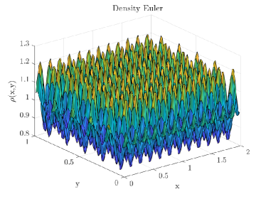
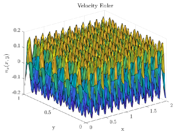
Refer to caption
Refer to caption
Figure 4.1: Highly oscillating fluid. Profiles of density (left) and first component of the velocity ux(x,y,t)subscript𝑢𝑥𝑥𝑦𝑡u_{x}(x,y,t) (right) at final time for the isentropic Euler equations.
Refer to caption
Refer to caption
Refer to caption
Refer to caption
Refer to caption
Refer to caption
Figure 4.2: Highly oscillating fluid. Comparison of the density (left) and velocity ux(x,y,t)subscript𝑢𝑥𝑥𝑦𝑡u_{x}(x,y,t) (right) profiles for x=0.5𝑥0.5x=0.5. The results for the Euler, the BGK and the HMM equations with respectively τ=0.001𝜏0.001\tau=0.001, τ=0.005𝜏0.005\tau=0.005 and τ=0.01𝜏0.01\tau=0.01 are shown.
Refer to caption
Refer to caption
Refer to caption
Refer to caption
Refer to caption
Refer to caption
Figure 4.3: Highly oscillating fluid. Comparison of the density (left) and velocity ux(x,y,t)subscript𝑢𝑥𝑥𝑦𝑡u_{x}(x,y,t) (right) profiles for x=0.5𝑥0.5x=0.5. The results for the the BGK, the Navier-Stokes and the HMM equations with respectively τ=0.001𝜏0.001\tau=0.001, τ=0.005𝜏0.005\tau=0.005 and τ=0.01𝜏0.01\tau=0.01 are shown.

4.4 Perturbed Couette flow

In this section, we consider a two-dimensional Couette-type flow in the domain Ω=[0,1]×[0,2]Ω0102\Omega=[0,1]\times[0,2] perturbed by high frequency waves. The setup is the following. The boundary conditions in the x𝑥x-direction are periodic while in the y𝑦y-direction we impose the so-called no-slip boundary conditions for which the normal to the walls velocity is fixed to zero while the tangential velocity is set equal to the velocity of the walls. The spatial domain is discretized as before with Nx×Ny=64×128subscript𝑁𝑥subscript𝑁𝑦64128N_{x}\times N_{y}=64\times 128 cells, while the velocity space is approximated by using 20×20202020\times 20 cells in the domain [5,5]2superscript552[-5,5]^{2}. Local equilibrium for the distribution function is supposed at time t=0𝑡0t=0. The initial density and velocities are

ρ(x,y,0)=1+0.2cos(10πx)sin(12πy),𝒖(x,y,0)=(ux,uy)=(y(1+0.125sin(8πx)),0).formulae-sequence𝜌𝑥𝑦010.210𝜋𝑥12𝜋𝑦𝒖𝑥𝑦0subscript𝑢𝑥subscript𝑢𝑦𝑦10.1258𝜋𝑥0\rho(x,y,0)=1+0.2\cos(10\pi x)\sin(12\pi y),\ \bm{u}(x,y,0)=(u_{x},u_{y})=(y(1+0.125\sin(8\pi x)),0).

In other words, we simulate a steady state Couette flow with an added high frequency perturbations both in the density and the velocity. In particular, to the top wall and in the y𝑦y-direction it is imposed an oscillatory velocity in the x𝑥x-direction which reads

uy(x,2,t)=1+0.25sin(8πx).subscript𝑢𝑦𝑥2𝑡10.258𝜋𝑥u_{y}(x,2,t)=1+0.25\sin(8\pi x).

The temperature and the universal gas constant are set T=1𝑇1T=1 and R=1𝑅1R=1 as before. In Figure 4.4, we show the density and the velocities profiles after 100100100 time iteration with a time step of Δt=6.25 104Δ𝑡superscript6.25104\Delta t=6.25\ 10^{-4}. At this time, the perturbed waves have not been completely damped out: it is still possible to observe how the oscillations in velocity and density modify the solution as the intensity of the relaxation parameter grows. In particular, Figure 4.4 shows the solutions obtained with τ=0𝜏0\tau=0, τ=0.005𝜏0.005\tau=0.005 and τ=0.01𝜏0.01\tau=0.01 for the BGK model, while for the HMM we take τHMM=τ/3subscript𝜏𝐻𝑀𝑀𝜏3\tau_{HMM}=\tau/3 as for the first test. In Figure 4.5, we present the same results at x=0.5𝑥0.5x=0.5 comparing the isentropic Euler, the BGK and the HMM solutions. In this picture, we can clearly see that oscillations are damped when moving far from the regime of validity of the isentropic Euler equations and that the HMM captures the BGK solution very well for all regimes, considered at least for the density and the first component of the velocity field. Finally, in Figure 4.6, we show a comparison between the HMM and the NS model using again the BGK model as reference, all presented at x=0.5𝑥0.5x=0.5. For the specific case of the NS model, we take ε=τ𝜀𝜏\varepsilon=\tau while all the others numerical parameters are equal to the ones of the HMM model. From this figure we see that for small values of τ𝜏\tau both models capture very well the reference solution given by the BGK equation, while for larger τ𝜏\tau, NS tends to overestimate the damping for what concerns the density profile. Both models is capable of capturing the first component of the velocity field uxsubscript𝑢𝑥u_{x}, while both fail in the description of the second component uysubscript𝑢𝑦u_{y} when τ=0.01𝜏0.01\tau=0.01. Let observe anyway that uysubscript𝑢𝑦u_{y} is affected by waves, which are at least one order of magnitude smaller than the perturbation waves acting on the other macroscopic quantities and thus the error introduced in the solution remains very small.
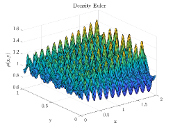
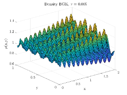
Refer to caption
Refer to caption
Refer to caption
Refer to caption
Refer to caption
Refer to caption
Refer to caption
Refer to caption
Refer to caption
Figure 4.4: Perturbed Couette flow. Profiles of density and velocity for the Euler and the BGK equations. From top to bottom: Density, x-velocity and y-velocity profiles. Left τ=0𝜏0\tau=0, middle τ=0.005𝜏0.005\tau=0.005, right τ=0.01𝜏0.01\tau=0.01.
Refer to caption
Refer to caption
Refer to caption
Refer to caption
Refer to caption
Refer to caption
Refer to caption
Refer to caption
Refer to caption
Figure 4.5: Perturbed Couette flow. Comparison of the density (left), x𝑥x-velocity (middle) and y𝑦y-velocity (right) profiles for x=0.5𝑥0.5x=0.5. The results for the Euler, the BGK and the HMM equations with respectively τ=0.001𝜏0.001\tau=0.001, τ=0.005𝜏0.005\tau=0.005 and τ=0.01𝜏0.01\tau=0.01 are shown.
Refer to caption
Refer to caption
Refer to caption
Refer to caption
Refer to caption
Refer to caption
Refer to caption
Refer to caption
Refer to caption
Figure 4.6: Perturbed Couette flow. Comparison of the density (left), x𝑥x-velocity (middle) and y𝑦y-velocity (right) profiles for x=0.5𝑥0.5x=0.5. The results for the the BGK, the Navier-Stokes and the HMM equations with respectively τ=0.001𝜏0.001\tau=0.001, τ=0.005𝜏0.005\tau=0.005 and τ=0.01𝜏0.01\tau=0.01 are shown.

4.5 A vortex test problem

In this last section, we consider a Taylor-Green-type problem. The initial data are given by

ρ(x,y,0)=1+0.1cos(8πx)sin(8πy),𝒖(x,y,0)=(ux,uy)=(cos(x)sin(y),cos(y)sin(x)).formulae-sequence𝜌𝑥𝑦010.18𝜋𝑥8𝜋𝑦𝒖𝑥𝑦0subscript𝑢𝑥subscript𝑢𝑦𝑥𝑦𝑦𝑥\rho(x,y,0)=1+0.1\cos(8\pi x)\sin(8\pi y),\ \bm{u}(x,y,0)=(u_{x},u_{y})=(\cos(x)\sin(y),-\cos(y)\sin(x)).

The temperature is T=1𝑇1T=1, the universal gas constant R=1𝑅1R=1, and the computational domain is Ω=[0,2π]2Ωsuperscript02𝜋2\Omega=[0,2\pi]^{2} discretized with Nx=Ny=128subscript𝑁𝑥subscript𝑁𝑦128N_{x}=N_{y}=128 points in each direction. The velocity space is discretized using the same parameters as in the previous tests. We take a time step Δt=2 104Δ𝑡superscript2104\Delta t=2\ 10^{-4} and set a final time of Tf=0.6subscript𝑇𝑓0.6T_{f}=0.6. The initial data are represented in Figure 4.7 on the top left, while the final solution for the isentropic Euler is reported in the same figure on the top right and illustrates the vortices formation. The bottom image reports a three-dimensional view of the same solution for the density. In Figure 4.8, we present comparisons between the isentropic Euler, the BGK and our HMM at the final time for the density and the velocities and for three different values of the relaxation parameter τ=0.005𝜏0.005\tau=0.005, τ=0.01𝜏0.01\tau=0.01 and τ=0.025𝜏0.025\tau=0.025 with τHMM=τ/3subscript𝜏𝐻𝑀𝑀𝜏3\tau_{HMM}=\tau/3. Once again, the obtained results indicate that the HMM is able to capture microscopic structures with a sufficiently high accuracy for the regimes under considaration.
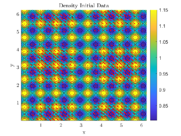
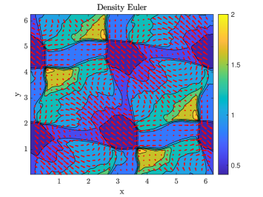
Refer to caption
Refer to caption
Refer to caption
Refer to caption
Figure 4.7: Vortex flow. Profiles of density and velocity for the Euler and the BGK equations. From top to bottom: Density initial data, density Euler solution, density Euler solution three dimensional view and density BGK solution with τ=0.01𝜏0.01\tau=0.01. Red arrows represent the velocity vector field.
Refer to caption
Refer to caption
Refer to caption
Refer to caption
Refer to caption
Refer to caption
Refer to caption
Refer to caption
Refer to caption
Figure 4.8: Vortex flow. Comparison of the density (left), x𝑥x-velocity (middle) and y𝑦y-velocity (right) profiles for x=0.5𝑥0.5x=0.5. The results for the Euler, the BGK and the HMM equations with respectively τ=0.005𝜏0.005\tau=0.005, τ=0.01𝜏0.01\tau=0.01 and τ=0.025𝜏0.025\tau=0.025 are shown.

5 Conclusions

In this work, we have introduced a new hybrid multiscale model coupling the continuum and kinetic descriptions. We have applied the Chapman-Enskog expansion on a suitably scaled stationary BGK equation and then upscaled the kinetic contribution over a microscopic box. These microscopic regions are located at each points where the fluid equation are solved. The probability density function used to study the kinetic evolution is related to the unknown density and velocity of the system through truncated Taylor expansions. Based on a scaling assumption, related to the problem under consideration, a new multiscale continuum-kinetic model has been derived. A linear stability analysis shows that new hybrid multiscale model is conditionally linearly stable in the strongly supersonic regime and unconditionally stable in the subsonic and mildly supersonic one. Several numerical examples demonstrate that the hybrid multiscale model is more accurate than standard fluid models and represents complex flows at different regimes more precisely.

In future work we would like to derive different hybrid multiscale models following the same general strategy outlined in this work: couple a microscopic description with a macroscopic one through an upscaling of the microscopic information obtained by homogenization of the micro quantities over micro sized boxes.

Acknowledgment:

The work of A. Chertock was supported in part by NSF grants DMS-1818684. P. Degond holds a visiting professor association with the Department of Mathematics, Imperial College London, UK. The work of G. Dimarco was supported by the Italian Ministry of Instruction, University and Research (MIUR) under the PRIN Project 2017 (No. 2017KKJP4X). M. Lukáčová-Medvid’ová and A. Ruhi were supported by the German Science Foundation (DFG) under the Collaborative Research Center TRR 146 Multiscale Simulation Methods for Soft Matter Systems (Project C5). M. Lukáčová-Medvid’ová is grateful to the Gutenberg Research College and Mainz Institute of Multiscale Modelling for supporting her research.

References

  • [1] U. M. Ascher, S. J. Ruuth, and R. J. Spiteri, Implicit-explicit Runge-Kutta methods for time-dependent partial differential equations, Appl. Numer. Math., 25 (1997), pp. 151–167. Special issue on time integration (Amsterdam, 1996).
  • [2] C. Bardos, F. Golse, and C. D. Levermore, Fluid dynamic limits of kinetic equations. II. Convergence proofs for the Boltzmann equation, Comm. Pure Appl. Math., 46 (1993), pp. 667–753.
  • [3] P. L. Bhatnagar, E. P. Gross, and M. Krook, A model for collision processes in gases. I. Small amplitude processes in charged and neutral one-component systems, Phys. Rev., 94 (1954), pp. 511–525.
  • [4] M. K. Borg, D. A. Lockerby, and J. M. Reese, Fluid simulations with atomistic resolution: a hybrid multiscale method with field-wise coupling, J. Comput. Phys., 255 (2013), pp. 149–165.
  • [5]  , A hybrid molecular–continuum method for unsteady compressible multiscale flows, J. Fluid Mech., 768 (2015), p. 388–414.
  • [6] C. Cercignani, Mathematical methods in kinetic theory, Plenum Press, New York, second ed., 1990.
  • [7] A. Crestetto, N. Crouseilles, G. Dimarco, and M. Lemou, Asymptotically complexity diminishing schemes (ACDS) for kinetic equations in the diffusive scaling, J. Comput. Phys., 394 (2019), pp. 243–262.
  • [8] R. Datta, L. Yelash, F. Schmid, F. Kummer, M. Oberlack, M. Lukáčová-Medviďová, and P. Virnau, Shear-thinning in oligomer melts-molecular origin and applications, Polymers, 13 (2021), p. 2806.
  • [9] P. Degond, G. Dimarco, and L. Pareschi, The moment-guided Monte Carlo method, Internat. J. Numer. Methods Fluids, 67 (2011), pp. 189–213.
  • [10] P. J. Dellar, Two routes from the Boltzmann equation to compressible flow of polyatomic gases, Prog. Comput. Fluid Dyn., 8 (2008), pp. 84–96.
  • [11] G. Dimarco and L. Pareschi, Fluid solver independent hybrid methods for multiscale kinetic equations, SIAM J. Sci. Comput., 32 (2010), pp. 603–634.
  • [12] G. Dimarco and L. Pareschi, Asymptotic preserving implicit-explicit Runge-Kutta methods for nonlinear kinetic equations, SIAM J. Numer. Anal., 51 (2013), pp. 1064–1087.
  • [13]  , Numerical methods for kinetic equations, Acta Numer., 23 (2014), pp. 369–520.
  • [14] W. E, Principles of multiscale modeling, Cambridge University Press, Cambridge, 2011.
  • [15] W. E and B. Engquist, The heterognous multiscale methods, Commun. Math. Sci., 1 (2003), pp. 87–132.
  • [16] W. E, B. Engquist, X. Li, W. Ren, and E. Vanden-Eijnden, Heterogeneous multiscale methods: A review, Commun. Comput. Phys., 2 (2007), pp. 367–450.
  • [17] W. E and X. Li, Analysis of the heterogeneous multiscale method for gas dynamics, Methods Appl. Anal., 11 (2004), pp. 557–572.
  • [18] W. E and J. Lu, Seamless multiscale modeling via dynamics on fiber bundles, Commun. Math. Sci., 5 (2007), pp. 649–663.
  • [19] W. E, P. Ming, and P. Zhang, Analysis of the heterogeneous multiscale method for elliptic homogenization problems, J. Amer. Math. Soc., 18 (2005), pp. 121–156.
  • [20] D. A. Fedosov and G. E. Karniadakis, Triple-decker: interfacing atomistic-mesoscopic-continuum flow regimes, J. Comput. Phys., 228 (2009), pp. 1157–1171.
  • [21] F. Golse and L. Saint-Raymond, The incompressible Navier-Stokes limit of the Boltzmann equation for hard cutoff potentials, J. Math. Pures Appl. (9), 91 (2009), pp. 508–552.
  • [22] H. Grad, Asymptotic equivalence of the Navier-Stokes and nonlinear Boltzmann equations, in Proc. Sympos. Appl. Math., Vol. XVII, Amer. Math. Soc., Providence, R.I., 1965, pp. 154–183.
  • [23] J. H. Irving and J. G. Kirkwood, he statistical mechanical theory of transport processes. IV. The equations of hydrodynamics, J. Chem. Phys., 18 (1950), pp. 508–552.
  • [24] Y. Ishida and T. Yamamoto, Linear And Nonlinear Rotordynamics: a modern treatment with applications, John Wiley & Sons, 2013.
  • [25] I. G. Kevrekidis, C. W. Gear, J. M. Hyman, P. G. Kevrekidis, O. Runborg, and C. Theodoropoulos, Equation-free, coarse-grained multiscale computation: enabling microscopic simulators to perform system-level analysis, Commun. Math. Sci., 1 (2003), pp. 715–762.
  • [26] I. G. Kevrekidis and G. Samaey, Equation-free multiscale computation: algorithms and applications, Annu. Rev. Phy.s Chem., 60 (2009), pp. 321–344.
  • [27] P. Koumoutsakos, Multiscale flow simulations using particles, vol. 37 of Annu. Rev. Fluid Mech., Palo Alto, 2005, pp. 457–487.
  • [28] C. D. Levermore and N. Masmoudi, From the Boltzmann equation to an incompressible Navier-Stokes-Fourier system, Arch. Ration. Mech. Anal., 196 (2010), pp. 753–809.
  • [29] F.-H. Lin, C. Liu, and P. Zhang, On hydrodynamics of viscoelastic fluids, Comm. Pure Appl. Math., 58 (2005), pp. 1437–1471.
  • [30] L. Mieussens, Discrete velocity model and implicit scheme for the BGK equation of rarefied gas dynamics, Mathematical Models and Methods in Applied Sciences, 10 (2000), pp. 1121–1149.
  • [31] J. Nečas and I. Hlaváček, Mathematical theory of elastic and elasto-plastic bodies: an introduction, vol. 3 of Studies in Applied Mechanics, Elsevier, 1980.
  • [32] G. A. Radtke, J.-P. M. Péraud, and N. G. Hadjiconstantinou, On efficient simulations of multiscale kinetic transport, Philos. Trans. R. Soc. Lond. Ser. A Math. Phys. Eng. Sci., 371 (2013), p. 20120182.
  • [33] K. K. Rao and P. R. Nott, An introduction to granular flow, Cambridge Series in Chemical Engineering, Cambridge University Press, 2008.
  • [34] W. Ren, Analytical and numerical study of coupled atomistic-continuum methods for fluids, J. Comput. Phys., 227 (2007), pp. 1353–1371.
  • [35]  , Seamless multiscale modeling of complex fluids using fiber bundle dynamics, Commun. Math. Sci., 5 (2007), pp. 1027–1037.
  • [36] W. Ren and W. E, Heterogeneous multiscale method for the modeling of complex fluids and micro-fluidics, J. Comput. Phys., 204 (2005), pp. 1–26.
  • [37] S. E. Spagnolie, ed., Complex fluids in biological systems, Biological and Medical Physics, Biomedical Engineering, Springer, New York, 2015. Experiment, theory, and computation.
  • [38] S. Stalter, L. Yelash, N. Emamy, A. Statt, M. Hanke, M. Lukáčová-Medviďová, and P. Virnau, Molecular dynamics simulations in hybrid particle-continuum schemes: Pitfalls and caveats, Comput. Phys. Commun., 224 (2018), pp. 198–208.
  • [39] F. Tedeschi, G. G. Giusteri, L. Yelash, and M. Lukáčová-Medviďová, A multi-scale method for complex flows of non-Newtonian fluids, Math. Eng., 4(6) (2022), pp. 1–22.
  • [40] S. Yasuda and R. Yamamoto, Multiscale modeling and simulation for polymer melt flows between parallel plates, Phys. Rev. E, 81 (2010), p. 036308.