The saddle-point exciton signature on high harmonic generation in 2D hexagonal nanostructures

Abstract

The disclosure of basic nonlinear optical properties of graphene-like nanostructures with correlated electron-hole nonlinear dynamics over a wide range of frequencies and pump field intensities is of great importance for both graphene fundamental physics and for expected novel applications of 2D hexagonal nanostructures in extreme nonlinear optics. In the current paper, the nonlinear interaction of 2D hexagonal nanostructures with the bichromatic infrared driving field taking into account many-body Coulomb interaction is investigated. Numerical investigation in the scope of the Bloch equations within the Houston basis that take into account $e-e$ and $e-h$ interactions in the Hartree-Fock approximation reveals significant excitonic effects in the high harmonic generation process in 2D hexagonal nanostructures such as graphene and silicene. It is shown that due to the correlated electron-hole nonlinear dynamics around the van Hove singularity, spectral caustics in the high harmonic generation spectrum are induced near the saddle point excitonic resonances.

I Introduction

Many of the optoelectronic properties of graphene [1] and its analog silicene [2, 3, 4] can be understood within a non-interacting free charged carrier picture. The most pronounced feature of these nanostructures is the characteristic linear dispersion relation of massless Dirac fermions [5] and the anomalous integer quantum Hall effect [6]. The measured optical conductivity up to the visible region is close to the value of $e^{2}/4\hbar$ [7] predicted within the free-particle (FP) theory [8]. On the other hand, since the screening length diverges at the charge neutrality point [1], one can expect the significant influence of the many-body electronic interactions on the properties of hexagonal nanostructures. Indeed, depending on the substrate material many-body electronic interactions lead to departure from the linear dispersion relation [9, 10, 11] and to the fractional quantum Hall effect [12, 13]. In graphene, the ratio of the Coulomb potential energy to the kinetic one, that is the Wigner-Seitz radius, is independent of density. The latter is defined as $r_{s}=e^{2}/(\hbar\mathrm{v}_{F}\epsilon)$, where $\epsilon$ is the background lattice dielectric constant of the system, $\mathrm{v}_{F}$ is the Fermi velocity. For intrinsic graphene $r_{s}\approx 2.4$ and since $r_{s}$ is also the ”effective fine structure constant” for graphene [9], this should result in considerable changes in graphene’s properties, including the opening of an energy gap [14, 15, 16]. Experimental evidence for such phenomena is absent. This discrepancy is resolved if one takes into account the screening stemming from the valence electrons, which is almost $4$ for intrinsic graphene [17]. The substrate-induced screening further suppresses Coulomb interaction making graphene a weakly interacting system. For example, the substrate SiO₂ reduces Wigner-Seitz radius to $r_{s}\approx 0.5$. At first glance this is a small value, however electron-electron interaction can also significantly modify the linear optical response of graphene-like materials due to excitonic effects [18, 19, 20, 21, 22, 23, 24, 25, 26]. These effects are significant near Van Hove singularity (VHS) [27] point in the Brillouin zone (BZ) giving rise to a pronounced peak in the optical absorption. Both the position and shape of this peak evidence the role of strong Coulomb interactions [18, 19, 20, 21]. Instead of simple free-free transitions, electron-hole correlated transitions take place. These are revealed in the absorption spectrum of graphene in the ultraviolet range. Note that for silicene the excitonic resonance is expected in the visible range of spectrum.

The significance of many-body Coulomb interaction has also been shown for ultrafast many-particle kinetics [28, 29, 30] and for the perturbative nonlinear optics in graphene [31, 32, 33, 34]. With the further increase of the pump wave intensity, one can enter into the extreme nonlinear optical regime [35], where high order harmonics generation (HHG) takes place. The HHG until the last decade has been the prerogative of atomic systems. But with the advent of graphene and other novel nanostructures, it becomes clear that HHG can be much more efficient in these materials. There are several investigations devoted to the HHG phenomenon in the monolayer [36, 37, 38, 39, 40, 41, 42, 43, 44], bilayer [45, 46, 47], and gapped graphene [48, 49] nanostructures with the pump wave of linear polarization. Since the observation of the HHG enhancement by the elliptically polarized light in graphene by Yoshikawa et al. [50] , the polarization and optical anisotropy effects of HHG in graphene have been attracting much interest [51, 52, 53, 54, 55, 56, 57, 58] as it is distinct from the HHG in gases where HHG is significantly suppressed with an increase of the ellipticity of a pump wave [59]. After successful adoption of three-step semiclassical model developed for atomic HHG [60] to gapped nanostructures [61, 62], there have been attempts to extend this model to graphene [44, 57, 63, 58].In the three-step semiclassical model, at the first step for the gapped system, there is a localization of the excited electron-hole wave packet in the BZ around the minimum bandgap at the instant of tunneling. For graphene, due to the vanishing bandgap depending on the intensity, polarization, and frequency of the pump wave different scenarios can occur. In particular, instead of the tunneling ionization/excitation the resonant one photon or/and multiphoton excitation of the Fermi-Dirac sea can take place [37], or the first step can be initiated by non-diabatic crossing [44] of the valence band electron trajectories through the Dirac points, where the transition dipole moment is singular. For graphene, as well as for other nanostructures one should also relax the condition for recombination [57, 58]. Due to the wave packet spreading an annihilation at a relative electron-hole distance comparable to lattice spacing, so-called imperfect recollision can take place [64]. With these modifications, one can explain the enhancement of HHG yield in the elliptically polarized laser fields [57] or in two-color laser fields at orthogonal polarizations [58].

Compared with the gaseous system there is also one important factor that can significantly modify the three-step semiclassical model. As has been shown in Ref. [65], at VHS spectral caustics are induced resulting in a strong amplification of the HHG signal. On the other hand, in graphen-like nanostructures near VHS the many-body Coulomb interaction is expected to be significant. Hence, it is of interest to clear up the signature of electron-electron interaction on the extreme nonlinear optical response of graphene-like nanostructures in the situation when the charged carriers are accelerated up to the $M$ saddle point in the BZ. The importance of Coulomb interaction for HHG in graphene has been previously predicted in Ref. [43]. The latter study was conducted near the Dirac points where excitonic effects are weak.

In the present work, we investigate the influence of saddle-point excitons on the HHG process in a 2D hexagonal nanostructure. The electron-electron Coulomb interaction is taken into account in the scope of the Hartree-Fock (HF) approximation applicable to the full BZ. This ansatz leads to a closed set of integrodifferential Bloch equations for the single-particle density matrix in the Houston basis. The carrier-carrier and carrier-phonon scatterings are taken into account phenomenologically with the relaxation term. As reference nanostructures, we consider graphene and silicene. For the latter, we neglect the small gap due to the spin-orbit coupling, which is irrelevant for the current study.

The paper is organized as follows. In Sec. II the model and the basic equations are formulated. In Sec. III, we present the main results. Finally, conclusions are given in Sec. IV.

II The model and a closed set of integro-differential equations

We consider the interaction of a strong laser field, bichromatic or monochromatic, with a two-dimensional hexagonal nanostructure such as graphene and silicene. The electric field strength of the considering wave-field can be written as:

$$\mathbf{E}\left(t\right)=f\left(t\right)E_{0}\left(\hat{\mathbf{e}}\cos\left(\omega_{0}t\right)+\hat{\mathbf{e}}^{\prime}\varepsilon\cos\left(\omega_{0}^{\prime}t-\varphi\right)\right),$$ (1)

where $f\left(t\right)=\sin^{2}\left(\pi t/\tau\right)$ is the sin-squared envelope function, $\tau$ is the pulse duration, $\hat{\mathbf{e}}$ and $\hat{\mathbf{e}}^{\prime}$ are unite polarization vectors in the plane of 2D nanostructure ($XY$), $\omega_{0}$ and $\omega_{0}^{\prime}$ are currier frequencies, $E_{0}$ is the amplitude, $\varepsilon$ and $\varphi$ are the relative amplitude and phase of the two waves, respectively. We take an eight-cycle fundamental laser field. In the HF approximation we reduce the electron-electron Coulomb interaction into the mean-field Hamiltonian [43]. As a result, we obtain a closed set of equations for the interband polarization $\mathcal{P}(\mathbf{k},t)=\mathcal{P}^{\prime}(\mathbf{k},t)+i\mathcal{P}^{\prime\prime}(\mathbf{k},t)$ and for the distribution functions $\mathcal{N}_{c/v}\left(\mathbf{k},t\right)$ of the conduction/valence bands. Then, one can obtain semiconductor Bloch equations in the HF approximation. We will consider the latter in the Houston basis, i.e. the crystal momentum $\mathbf{k}$ is transformed into a frame moving with the vector potential $\mathbf{k}_{0}=\mathbf{k}-\mathbf{A}$, where $\mathbf{A=-}\int_{0}^{t}\mathbf{E}\left(t^{\prime}\right)dt^{\prime}$ is the vector potential and $\mathbf{E}$ is the laser electric field strength. For compactness of equations atomic units are used throughout the paper unless otherwise indicated. On the HF level for an undoped system in equilibrium, the initial conditions $\mathcal{P}(\mathbf{k},0)=0$, $N_{c}(\mathbf{k},0)=0$, and $N_{v}(\mathbf{k},0)=1$ are assumed, neglecting thermal occupations. In this case the equation for $N_{v}(\mathbf{k},t)$ is superficial. Thus, the Bloch equations with damping ($\Gamma$) within the Houston basis read

$$\partial_{t}\mathcal{N}_{c}(\mathbf{k}_{0},t)=-2\mathrm{Im}\left\{\left[\mathbf{E}\left(t\right)\mathbf{D}_{\mathrm{tr}}\left(\mathbf{k}_{0}+\mathbf{A}\right)\right.\right.$$

$$\left.\left.+\Omega_{c}\left(\mathbf{k}_{0}+\mathbf{A},t;\mathcal{P},\mathcal{N}_{c}\right)\right]\mathcal{P}^{\ast}(\mathbf{k}_{0},t)\right\},$$ (2)

$$\partial_{t}\mathcal{P}(\mathbf{k}_{0},t)=-i\left[\mathcal{E}_{eh}\left(\mathbf{k}_{0}+\mathbf{A}\right)-i\Gamma\right]\mathcal{P}(\mathbf{k}_{0},t)$$

$$+i\left[\mathbf{E}\left(t\right)\mathbf{D}_{\mathrm{tr}}\left(\mathbf{k}_{0}+\mathbf{A}\right)+\Omega_{c}\left(\mathbf{k}_{0}+\mathbf{A},t;\mathcal{P},\mathcal{N}_{c}\right)\right]$$

$$\times\left[1-2\mathcal{N}_{c}(\mathbf{k}_{0},t)\right],$$ (3)

where

$$\mathcal{E}_{eh}\left(\mathbf{k}\right)=2\mathcal{E}\left(\mathbf{k}\right)-\Xi_{c}(\mathbf{k},t;\mathcal{P},\mathcal{N}_{c})$$ (4)

is the electron-hole energy defined via the band energy

$$\mathcal{E}\left(\mathbf{k}\right)=\gamma_{0}\left|f\left(\mathbf{k}\right)\right|,$$ (5)

and many-body Coulomb interaction energy

$$\Xi_{c}(\mathbf{k},t;\mathcal{P},\mathcal{N}_{c})=\frac{2}{\left(2\pi\right)^{2}}\int_{BZ}d\mathbf{k}^{\prime}V_{2D}\left(\mathbf{k-k}^{\prime}\right)$$

$$\times\left\{f_{c}\left(\mathbf{k,k}^{\prime}\right)\mathcal{N}_{c}\left(\mathbf{k}^{\prime}\right)+f_{s}\left(\mathbf{k,k}^{\prime}\right)\mathcal{P}^{\prime\prime}\left(\mathbf{k}^{\prime},t\right)\right\}.$$ (6)

In Eqs. (5) $\gamma_{0}$ is the transfer energy of the nearest-neighbor hopping and the structure function is

$$f\left(\mathbf{k}\right)=e^{i\frac{ak_{y}}{\sqrt{3}}}+2e^{-i\frac{ak_{y}}{2\sqrt{3}}}\cos\left(\frac{ak_{x}}{2}\right),$$ (7)

where $a$ is the lattice spacing. In Eq. (6)

$$f_{c}\left(\mathbf{k,k}^{\prime}\right) = \cos\left[\mathrm{arg}f\left(\mathbf{k}^{\prime}\right)-\mathrm{arg}f\left(\mathbf{k}\right)\right],$$

$$f_{s}\left(\mathbf{k,k}^{\prime}\right) = \sin\left[\mathrm{arg}f\left(\mathbf{k}^{\prime}\right)-\mathrm{arg}f\left(\mathbf{k}\right)\right].$$

The electron-electron interaction potential is modelled by screened Coulomb potential [29]:

$$V_{2D}\left(\mathbf{q}\right)=\frac{2\pi}{\epsilon\epsilon_{\mathbf{q}}\left|\mathbf{q}\right|},$$ (8)

which accounts for the substrate-induced screening in the 2D nanostructure ($\epsilon$) and the screening stemming from valence electrons ($\epsilon_{\mathbf{q}}$). In Eqs. (2) and (3) the interband transitions are defined via the transition dipole moment

$$\mathbf{D}_{\mathrm{tr}}\left(\mathbf{k}\right)=-\frac{a}{2\left|f\left(\mathbf{k}\right)\right|^{2}}\sin\left(\frac{\sqrt{3}}{2}ak_{y}\right)\sin\left(\frac{ak_{x}}{2}\right)\widehat{\mathbf{x}}$$

$$+\frac{a}{2\sqrt{3}\left|f\left(\mathbf{k}\right)\right|^{2}}\left(\cos\left(ak_{x}\right)-\cos\left(\frac{\sqrt{3}}{2}ak_{y}\right)\cos\left(\frac{ak_{x}}{2}\right)\right)\widehat{\mathbf{y}},$$ (9)

and the light-matter coupling via the internal dipole field of all generated electron-hole excitations:

$$\Omega_{c}\left(\mathbf{k},t;\mathcal{P},\mathcal{N}_{c}\right)=\frac{1}{\left(2\pi\right)^{2}}\int_{BZ}d\mathbf{k}^{\prime}V_{2D}\left(\mathbf{k-k}^{\prime}\right)$$

$$\times\left\{\mathcal{P}^{\prime}\left(\mathbf{k}^{\prime},t\right)+if_{c}\left(\mathbf{k,k}^{\prime}\right)\mathcal{P}^{\prime\prime}\left(\mathbf{k}^{\prime}\right)-if_{s}\left(\mathbf{k,k}^{\prime}\right)\mathcal{N}_{c}\left(\mathbf{k}^{\prime},t\right)\right\}.$$ (10)

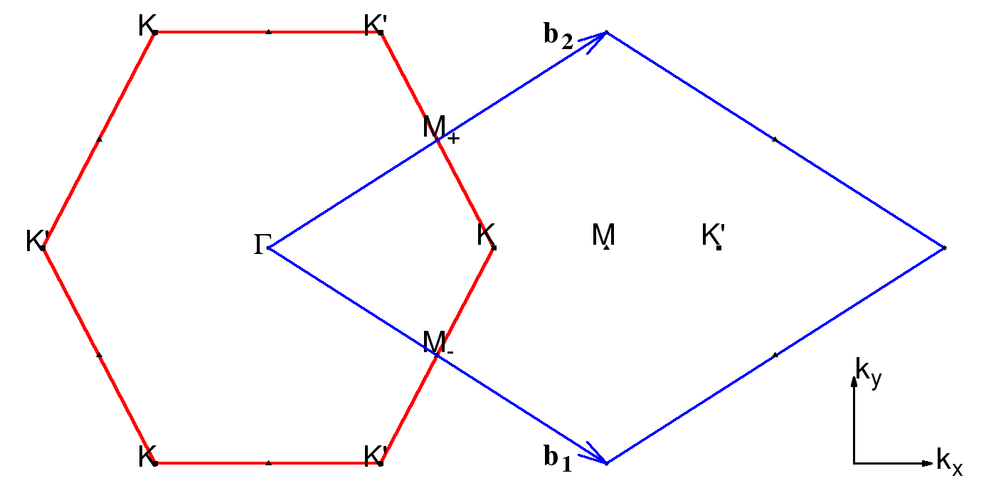
Figure 1: The hexagonal first BZ of the reciprocal lattice with high-symmetry points. The rhombus formed by the reciprocal lattice vectors is a reduction of the second BZ and contains the same vectors of the first BZ.

The electromagnetic response in 2D hexagonal nanostructure is determined by an intraband $\mathbf{j}_{a}\left(t\right)$ and interband $\mathbf{j}_{e}\left(t\right)$ contributions, which are given by

$$\mathbf{j}_{a}\left(t\right)=-\frac{4}{(2\pi)^{2}}\int_{\widetilde{BZ}}d\mathbf{k}_{0}\left[\mathbf{v}_{c}\left(\mathbf{k}_{0}+\mathbf{A}\right)\mathcal{N}_{c}\left(\mathbf{k}_{0},t\right)\right],$$ (11)

$$\mathbf{j}_{e}\left(t\right)=-\frac{4}{(2\pi)^{2}}\int_{\widetilde{BZ}}d\mathbf{k}_{0}\mathrm{Re}\left[\mathbf{v}_{\mathrm{tr}}^{\ast}\left(\mathbf{k}_{0}+\mathbf{A}\right)\mathcal{P}(\mathbf{k}_{0},t)\right],$$ (12)

respectively, where the band velocity is defined by $\mathbf{v}_{c}\left(\mathbf{k}\right)=\partial\mathcal{E}\left(\mathbf{k}\right)/\partial\mathbf{k}$, and $\mathbf{v}_{\mathrm{tr}}\left(\mathbf{k}\right)=2i\mathcal{E}\left(\mathbf{k}\right)\mathbf{D}_{\mathrm{tr}}\left(\mathbf{k}\right)\$is the transition matrix element for velocity. The Brillouin zone is also shifted to $\widetilde{BZ}=BZ-\mathbf{A}$.

The obtained Eqs. (2) and (3) formulate a closed set of integro-differential equations. We will solve these equations numerically. It is more convenient to make integration of these equations in the reduced BZ which contains equivalent $k$-points of the first BZ, cf. Fig. 1. The sampling $\mathbf{k}$-points are distributed homogeneously in the reduced BZ according to Monkhorst and Pack mesh. For the convergence of the results we take $500\times 500$ $\mathbf{k}$-points running parallel to the reciprocal lattice vectors: $\mathbf{b}_{1}=\left(\sqrt{3}k_{b}/2,-k_{b}/2\right)$ and $\mathbf{b}_{2}=\left(\sqrt{3}k_{b}/2,k_{b}/2\right)$, where $k_{b}=4\pi/\sqrt{3}a$. In the reduced BZ the low-energy excitations are centered around the two points $\mathrm{K}\left(k_{b}/\sqrt{3},0\right)$ and $\mathrm{K}^{\prime}\left(2k_{b}/\sqrt{3},0\right)$. The saddle point is $\mathrm{M}\left(\sqrt{3}k_{b}/2,0\right)$. The time integration is performed with the standard fourth-order Runge-Kutta algorithm. For sufficiently large 2D sample, when generated fields are considerably smaller than the pump field $\left|\mathbf{E}^{(g)}\right|\ll\left|\mathbf{E}\right|$, the generated electric field far from the hexagonal layer is proportional to the surface current: $\mathbf{E}^{(g)}(t)=-2\pi[\mathbf{j}_{e}(t)+\mathbf{j}_{a}(t)]/c$ [43]. For graphene/silicene on a substrate with a refractive index of $n_{s}$, it is also necessary to take into account the reflection of the incident wave [8] and rescale the driving and the generated fields by a factor of $2/(1+n_{s})$. The HHG spectral intensity is calculated from the fast Fourier transform of the generated field $\mathbf{E}^{(g)}(\omega)$. For the substrate-induced screening, we take $\epsilon=2.5$ that is close to the value of a graphene layer on a SiO₂ substrate ($n_{s}\simeq 2$). The screening induced by nanostructure valence electrons is calculated within the Lindhard approximation of the dielectric function $\epsilon_{\mathbf{q}}$.

III Results

The Coulomb contribution (6) in Eq. (3) describes the renormalization of the single-particle energy $\mathcal{E}\left(\mathbf{k}\right)$ due to the repulsive electron-electron interaction. Note that in the HF level we have neglected exchange interaction which is much smaller compared to direct Coulomb term [66]. Since we consider an undoped system, the exchange-correlation energy can also be neglected [67]. Note that the Coulomb-induced constant self-energy has been absorbed into the definition of the single-particle energy. At that, we will fix the tight-binding parameter $\gamma_{0}$ to obtain a good description of high energies near VHS without loss of accuracy around the $K$ point. The Coulomb contribution (10) in Eq. (2) accounts for electron-hole attraction. This term gives rise to so-called saddle-point exciton [18, 19, 20, 21] near the VHS of hexagonal BZ. To validate our theory within the limit of linear optics we first calculate the conductivity for graphene ($\gamma_{0}\simeq 0.1\ \mathrm{a.u.}$ and $a=4.64\ \mathrm{a.u.}$) and for silicene ($\gamma_{0}=0.04\ \mathrm{a.u.}$ and $a=7.28\ \mathrm{a.u.}$). We assume the linearly polarized ($\hat{\mathbf{e}}=\left\{1,0\right\}$, $\varepsilon=0$) laser with field strength $E\left(t\right)=f\left(t\right)E_{0}\cos\left(\omega t\right)$. The conductivity can be expressed as a function of the Fourier transform of the current density $\mathbf{j}\left(t\right)=\mathbf{j}_{a}\left(t\right)+\mathbf{j}_{e}\left(t\right)$ and the field strength:

$$\sigma\left(\omega\right)=\frac{j_{x}\left(\omega\right)}{E\left(\omega\right)}.$$ (13)

In Fig 2. we plot the FP and excitonic absorption spectrum via the real part of the conduction $\sigma\left(\omega\right)$ versus laser field frequency normalized to a universal one $\sigma_{0}=e^{2}/4\hbar$. From this figure we see the characteristic redshifting in the excitonic absorption spectrum with respect to the VHS peak expected in the scope of the FP picture. We also see the asymmetric shape that arises from the overlap with the free-particle transition. Due to ultrashort nature of the driving pulse the maximum value and the widths of the peaks are somewhat different than in the case of monochromatic wave [8].

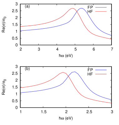
Figure 2: Free-particle and excitonic absorption spectrum via the real part of the conduction $\sigma\left(\omega\right)$ normalized to universal one $\sigma_{0}$ for graphene (a) and for silicene (b). We take an eight-cycle laser field with the amplitude $E_{0}=10^{-5}\ \mathrm{a.u.}$ and the relaxation rate is taken to be $\Gamma=5\times 10^{-4}\ \mathrm{a.u.}$. The excitonic absorption spectrum is redshifted with respect to the VHS peak expected in the scope of the free-particle picture.

The significant changes in the absorption line shape and peak position near the saddle point can be explained by the electron-hole interaction [18]. The saddle-point excitonic resonances (SPER) have been extensively investigated theoretically [68, 69, 70, 71, 72]. The changes in the absorption line shape can be understood from the band energy near the $M$ -point. Near the saddle point $k_{M}=\left(\sqrt{3}k_{b}/2,0\right)$ the band energy can be expanded as

$$\mathcal{E}\left(\mathbf{k}_{M}+\delta\mathbf{k}\right)=\gamma_{0}+\frac{\delta k_{x}^{2}}{2m_{x}}+\frac{\delta k_{y}^{2}}{2m_{y}},$$ (14)

where $m_{x}=-2/\left(\gamma_{0}a^{2}\right)\$and $m_{y}=2/\left(3\gamma_{0}a^{2}\right)$. That is, along the $K-M$ direction ($x$) the effective mass is negative, while along the $\Gamma-M$ direction ($y$) the effective mass is positive. In Fig. 3, we show the band structure and directions with effective masses of opposite signs. From the attractive electron-hole interaction the development of quasi-discrete excitonic states lying below the saddle-point singularity takes place, as is schematically shown in Fig. 3. The exciton binding energy is the energy difference from the SPER to the VHS calculated in the FP model. In our model, from Fig. 2, we find binding energies of about $500\ \mathrm{meV}$ and $250\ \mathrm{meV}$ for graphene and silicene, respectively. For graphene the obtained value is close to experimental one [18, 20]. Although the electron-hole interaction is attractive, the negative mass is equivalent to repulsion and in the perpendicular direction these excitonic states do not lie below a true gap. They consequently couple to the continuum formed by the band descending from the saddle point. By this reason the overall absorption line shape can be interpreted in terms of a Fano interference [72, 74, 73] effect.

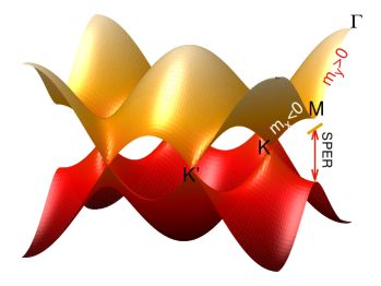
Figure 3: The band structure of hexagonal nanostructure. The valence and conduction bands cross at the $K$ and $K^{\prime}$ points. Near the saddle point $M$ we show SPER and the band dispersion along the $K-M$ and $\Gamma-M$ directions with effective masses of opposite signs.

Another feature of the excitonic resonance is the $\mathbf{k}$-space redistribution [21] of the oscillator strength which is defined by the interband polarization $\mathcal{P}(\mathbf{k},t)$. The excitonic states are defined from Eq. (3) when the pump field and relaxation rate are set to zero:

$$i\partial_{t}\mathcal{P}(\mathbf{k},t)=\mathcal{E}_{eh}\left(\mathbf{k}\right)\mathcal{P}(\mathbf{k},t)-\Omega_{c}\left(\mathbf{k},t;\mathcal{P},0\right).$$ (15)

This is the Bethe-Salpeter equation. For the excitonic states, the solution $\mathcal{P}(\mathbf{k},t)$ becomes more delocalized (localized) in the $\mathbf{k}$-space ($\mathbf{r}$-space) compared with the free particle states. This effect along with coupling of excitonic states with the continuum increases absorption below the SPER frequencies, cp. Fig. 2. These effects can strongly affect the interband current (12) also in strong-field interaction regime. Hence, it is of interest to clear up the signature of SPER on the extreme nonlinear optical response of the system, when the generated harmonics’ frequencies are near those resonances. In the HHG process the frequency of the emitted harmonic is defined by the electron-hole $\mathcal{E}_{eh}\left(\mathbf{k}_{0}+\mathbf{A}\right)$ energy which include kinetic energy acquired in the laser field, band gap and also Coulomb interaction energy. That is, prior to electron-hole annihilation their trajectories in the $\mathbf{k}$-space should be close to the saddle point $M$.

Thus, to enhance excitonic effects there are two possibilities: to excite the system with the photon of energy near $2\gamma_{0}$ [63] or when photon energy is much smaller than $\gamma_{0}$ to accelerate electrons/holes pair created near the Dirac points up to the energies $\gamma_{0}$. In the latter case, the trajectory in the $\mathbf{k}$-space should pass close to the $M$ point along the positive mass direction. The trajectory in the $\mathbf{k}$-space is the Lissajous diagram of the corresponding vector potential $\mathbf{A}$. In the case of linear polarization, this is impossible. In the case of circular/elliptic polarization, the trajectory in the $\mathbf{k}$-space can be close to the $M$ point but being far from the Dirac point, which is the source of electron-hole pairs [44]. For elliptic/circular polarization, the initial electron-hole pairs can be produced by a resonant one photon or/and multiphoton excitation of the Fermi-Dirac sea. However, for elliptic, and especially for circular polarization of the pump wave, there is a shortage of re-encountering electron-hole trajectories which is necessary for the high-probability annihilation. For modest ellipticity $\varepsilon\simeq 0.3$, the efficiency of the moderately high harmonics, where intraband current (11) is significant, can be enhanced [50]. However for interband current, where SPER is expected, we need fields with $\varepsilon\simeq 1$, since in the $\Gamma-M$ direction we expect constructive interference of many trajectories [65], cp. Fig. 9. Thus, one should choose a more sophisticated polarization of the driving waves. The latter can be achieved via a bichromatic driving field that is composed of the superposition of a fundamental pulse of linear polarization and its harmonic at the orthogonal polarization. In the case of the second harmonic, one may have ”Infinity” sign-like figure in the $\mathbf{k}$-space that at the sufficient intensity can pass through both $K$ and $M$ points. In this case, it will approach the point $M$ in the direction $\Gamma-M$. Indeed, this intuitive picture is validated with the numerical simulations: with the mid-infrared pump pulses, we can see the fingerprint of the SPER on the high harmonics.

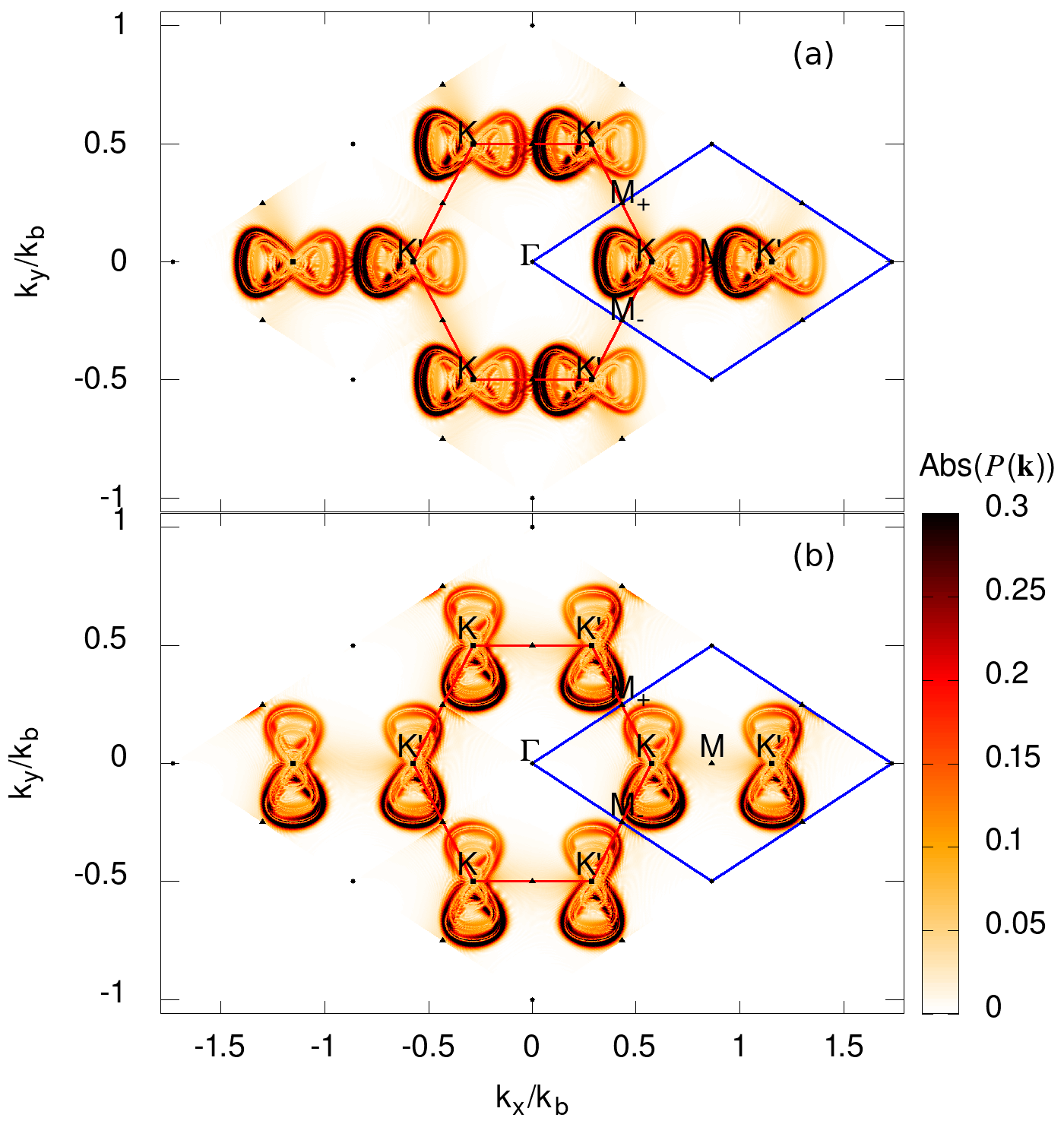
Figure 4: The density plot of the absolute value of the interband polarization (in arbitrary units) at the middle of interaction time ($t=\tau/2$) in bichromatic laser field for $\hat{\mathbf{e}}=\left\{1,0\right\}$, $\hat{\mathbf{e}}^{\prime}=\left\{0,1\right\}$ (a) and for $\hat{\mathbf{e}}=\left\{0,1\right\}$, $\hat{\mathbf{e}}^{\prime}=\left\{1,0\right\}$ (b) as a function of scaled dimensionless momentum components ($k_{x}/k_{b}$, $k_{y}/k_{b}$). The fundamental frequency is $\omega_{0}=0.1\ \mathrm{eV}/\hbar$, $\omega_{0}^{\prime}=2\omega_{0}$, $\varepsilon=1$, $\varphi=0$, and the interaction parameter is $\chi_{0}=1.7$. The first BZ (red hexagon) with high symmetry points and reduced BZ (blue rhomb) are also shown.

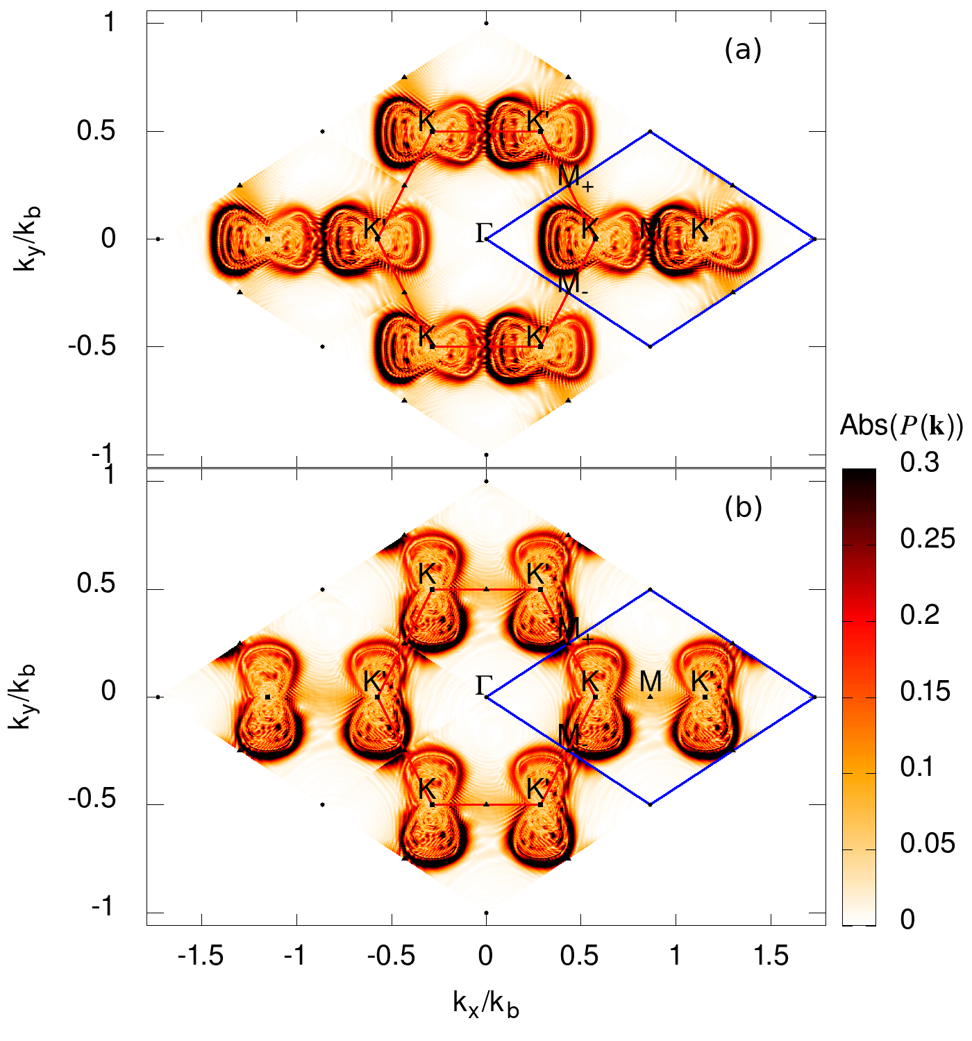
Figure 5: The same as in Fig. (4), but for silicene.

The wave-particle interaction will be characterized by the dimensionless parameter $\chi_{0}=eE_{0}a/\hbar\omega_{0}$ which represents the work of the wave electric field $E_{0}$ on a lattice spacing in the units of photon energy $\hbar\omega_{0}$. The parameter is written here in general units for clarity. The total intensity of the laser beam expressed by $\chi_{0}$, taking into account the reflectivity of the substrate, can be estimated as:

$$I_{\chi_{0}}=\chi_{0}^{2}\left(1+\varepsilon^{2}\right)\left(1+n_{s}\right)^{2}$$

$$\times[\hbar\omega_{0}/\mathrm{eV}]^{2}\times\left[\mathrm{\mathring{A}}/a\right]^{2}\times 3.3\times 10^{12}\ \mathrm{W\ cm}^{-2}.$$ (16)

The amplitude ($A_{0}$) of vector potential can be expressed in terms of the interaction parameter and reciprocal lattice spacing $k_{b}$ as $A_{0}=\chi_{0}k_{b}\left(\sqrt{3}/4\pi\right)$. Thus, with an increase in $\chi_{0}$ we can approach the point $M$ and thereby excite saddle-point excitons. The parameter $\chi_{0}$ is varied up to $2$ and frequency up to $0.2\ \mathrm{eV}/\hbar$. Hence, the maximal intensity $\,\allowbreak 1.57\ \mathrm{TW/cm}^{2}$ impending on graphene is below the damage threshold [50]. For silicene, due to larger lattice spacing the maximal intensity is almost $2.5$ times smaller. In this paper, we consider a two-band model formed from only $\pi$ orbitals. As a result, we neglect transitions in $\sigma$ and between $\pi-\sigma$ orbitals. These orbitals are separated from $\pi$ orbitals by a large energy gap of $\sim 3\gamma_{0}$. Hence, we should restrict the pump wave field strength by the condition $eE_{0}a<<3\gamma_{0}$, which is equivalent to $\chi_{0}<<3\gamma_{0}/\hbar\omega_{0}$.

First we consider a bichromatic laser field with $\omega_{0}^{\prime}=2\omega_{0}$, $\hat{\mathbf{e}}=\left\{1,0\right\}$, $\hat{\mathbf{e}}^{\prime}=\left\{0,1\right\}$, $\varphi=0$, and $\varepsilon=1$. At these parameters the vector potential corresponding to the field (1) draws $\infty-$like shape. In Figs. 4(a) and 5(a) the absolute value of the interband polarization $\left|\mathcal{P}(\mathbf{k})\right|$ is shown at the middle of interaction time ($t=\tau/2$) for graphene and silicene, respectively. It is clearly seen that the excitation patterns in the Fermi-Dirac sea follow the Lissajous diagram of the vector potential. At that, the surrounding of the $M$ point is excited in the $\Gamma-M$ direction and we expect the strong influence of this fact on the HHG spectra. One can also consider the bichromatic crossed fields when the polarizations are interchanged. In this case, we will have a vector potential drawing eight-like shapes. As a result, the excitations of $M_{+}$ and $M_{-}$saddle points will take place. These cases are shown in Figs. 4(b) and 5(b).

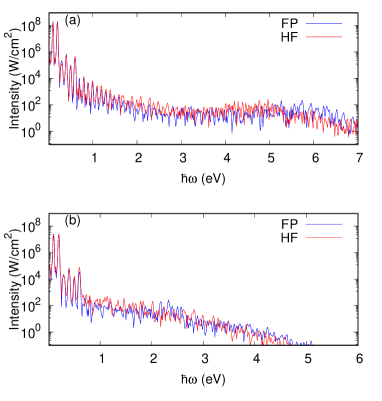
Figure 6: The HHG spectra in logarithmic scale for graphene (a) and for silicene (b) in the strong-field regime in the bichromatic driving field. The fundamental frequency is $\omega_{0}=0.1\ \mathrm{eV}/\hbar$ and the interaction parameter is $\chi_{0}=1.7$. The relaxation time is taken to be $\Gamma^{-1}=2\pi/\omega_{0}\simeq 40\ \mathrm{fs.}$

In Fig. 6, the HHG spectra in logarithmic scale with $\omega+2\omega$ frequency mixing for graphene and silicene in the strong-field regime is presented. We have also plotted the HHG spectra obtained in the scope of FP model. As is seen from this figure, the intensity of high-harmonics are enhanced near the frequencies close to SPER. For graphene, this is $4-5.0\ \mathrm{eV}$ and for silicene $1.5-2.0\ \mathrm{eV}$. The plateau peak is redshifted compared with the free-particle case. For the beginning of the spectrum where the intraband current (11) is dominant, the differences with the free carrier picture are not so noticeable. We also need a time-frequency analysis of the high harmonic spectrum for mapping the harmonics near saddle-point excitonic resonances with the Lissajous diagram of the vector potential. To this end, for graphene we perform the Morlet transform ($\sigma=4\pi$) of the interband part of the surface current (12):

$$\mathbf{J}\left(t,\omega\right)=\sqrt{\frac{\omega}{\sigma}}\int_{0}^{\tau}dt^{\prime}\mathbf{j}_{e}\left(t^{\prime}\right)e^{i\omega\left(t^{\prime}-t\right)}e^{-\frac{\omega^{2}}{2\sigma^{2}}\left(t^{\prime}-t\right)^{2}}.$$ (17)

The spectrogram, in a time interval where the waves’ amplitudes are considerable, is shown in Fig. 7 along with the Lissajous diagram of the vector potential. The laser parameters correspond to Fig. 6(a). The numbers over the spectrogram indicate the spectral caustics near the SPER. These caustics take place with the period $0.5T$ starting at $t\approx 3.75T$. The corresponding points are shown on the Lissajous diagram of the vector potential. As is clear from this mapping and also from Figs. 4 and 5, the spectral caustics near SPER originate when electron-hole pair move in $\mathbf{k}$-space along $\Gamma-M$ direction. Note that in this direction the band velocity $v_{x}\left(\frac{2\pi}{a},k_{y}\right)=\partial\mathcal{E}\left(\mathbf{k}\right)/\partial k_{x}=0$ irrespective of $k_{y}$, the discrete states in $k_{y}$ direction further flatten the band near the saddle point making $v_{y}\simeq 0$. That is, near the $\Gamma-M$ direction the relative semi-classical velocity between the electron and the hole vanishes, leading to a significant enhancement in their annihilation rate [65].

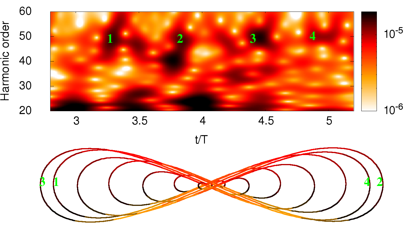
Figure 7: The spectrogram (color box in arbitrary units)) of the HHG process via the wavelet transform of the interband part of the surface current for graphene. The lower panel shows the Lissajous diagram of the vector potential. The laser parameters correspond to Fig. 6(a). The numbers over the spectrogram and Lissajous diagram indicate the spectral caustics near the SPER.

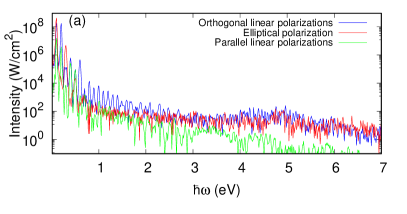
Figure 8: The HHG spectra in logarithmic scale for graphene in the strong-field regime for various polarizations of driving waves. The relaxation time is taken to be $\Gamma^{-1}=2\pi/\omega_{0}\simeq 40\ \mathrm{fs.}$ The fundamental frequency is $\omega_{0}=0.1\ \mathrm{eV}/\hbar$. The intensities (16) for all cases are equal. The interaction parameter for the orthogonal and parallel polarization cases is $\chi_{0}=1.7$.

To clarify the SPER signature in HHG spectra further, in particular with respect to the polarization of driving waves, we also made numerical calculations for the elliptical polarization of the laser field: $\omega_{0}^{\prime}=\omega_{0}$, $\hat{\mathbf{e}}=\left\{1,0\right\}$, $\hat{\mathbf{e}}^{\prime}=\left\{0,1\right\}$, $\varphi=\pi/2$, $\varepsilon=0.32$, and for the parallel linear polarizations of the bichromatic laser field: $\omega_{0}^{\prime}=2\omega_{0}$, $\hat{\mathbf{e}}=\hat{\mathbf{e}}^{\prime}=\left\{1,0\right\}$, $\varphi=0$, and $\varepsilon=1$. The results are shown in Fig. 8. For all three cases, we take the same intensity of $0.3\ TW/cm^{2}$. As is seen from this figure, in the case of parallel linear polarization there is no enhancement near the SPER. In the case of elliptic polarization, we have an enhancement in comparison to linear polarization. However, the orthogonal polarization case is preferable. For a qualitative understanding of this result, we also made a semi-classical trajectory analysis taking into account the actual excitation of the Fermi-Dirac sea, cp. Fig. 4. For the set of $\mathbf{k}_{0}$ points in the region $\mathcal{E}_{eh}\left(\mathbf{k}_{0}\right)\leq 3\ \mathrm{eV}$ we integrated the equation $\mathbf{r}_{e}\left(t^{\prime},t\right)=\int_{t^{\prime}}^{t}\left[\mathbf{v}_{c}\left(\mathbf{k}_{0}+\mathbf{A}\left(t^{\prime\prime}\right)\right)\right]dt^{\prime\prime}$ and calculated the electron-hole distance $\rho\left(t^{\prime},t\right)=\left|\mathbf{r}_{e}-\mathbf{r}_{h}\right|=2\left|\mathbf{r}_{e}\right|$. We kept only those trajectories for which at $t>t^{\prime}$ there is a local minimum of the electron-hole distance $\rho_{m}\left(t^{\prime},t\right)<2a$, i.e. we have at list imperfect collision [64]. Then we fixed the time and the corresponding energies $\mathcal{E}_{eh}\left(\mathbf{k}_{0}+\mathbf{A}\left(t\right)\right)$. In Fig. 9, we plot the colliding trajectories that in the semiclassical picture contribute to the caustic 2 indicated in Fig. 7 for the orthogonal and elliptic polarization cases. As is seen from Fig. 9(a), in the orthogonal polarization case the spectrum is dictated by the constructive interference of many trajectories, while in the case of elliptic polarization, Fig. 9(b) there is a shortage of re-encountering electron-hole trajectories.

Figure 9: Colliding trajectories. (a) The electron-hole distance as a function of time for the trajectories which collide in the time interval corresponding to the caustic 2 indicated in Fig. 7. The colored trajectory and colored box show the energies acquired by carriers along the trajectory. (b) The same as in (a) but for the elliptical polarization of the driving wave with the parameters corresponding to Fig. 8.

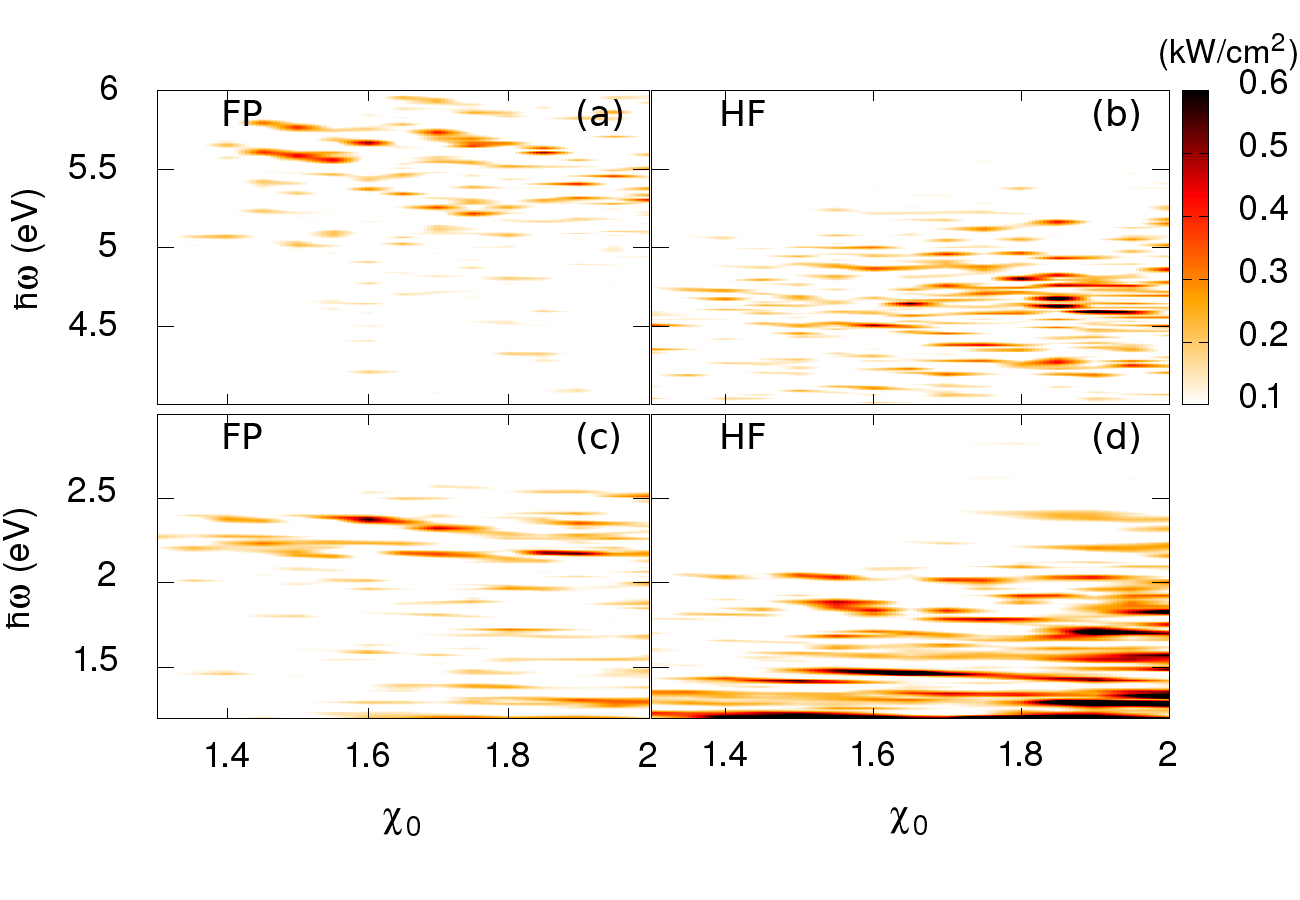
Figure 10: The intensity of HHG as a function of the interaction parameter and harmonic’s photon energy for graphene (a,b) and silicene (c,d) in the strong-field regime in the bichromatic driving field: $\omega_{0}=0.1\ \mathrm{eV}/\hbar$, $\omega_{0}^{\prime}=2\omega_{0}$, $\hat{\mathbf{e}}=\left\{1,0\right\}$, $\hat{\mathbf{e}}^{\prime}=\left\{0,1\right\}$, $\varphi=0$, and $\varepsilon=1$ . The relaxation time is taken to be $\Gamma^{-1}=40\ \mathrm{fs.}$

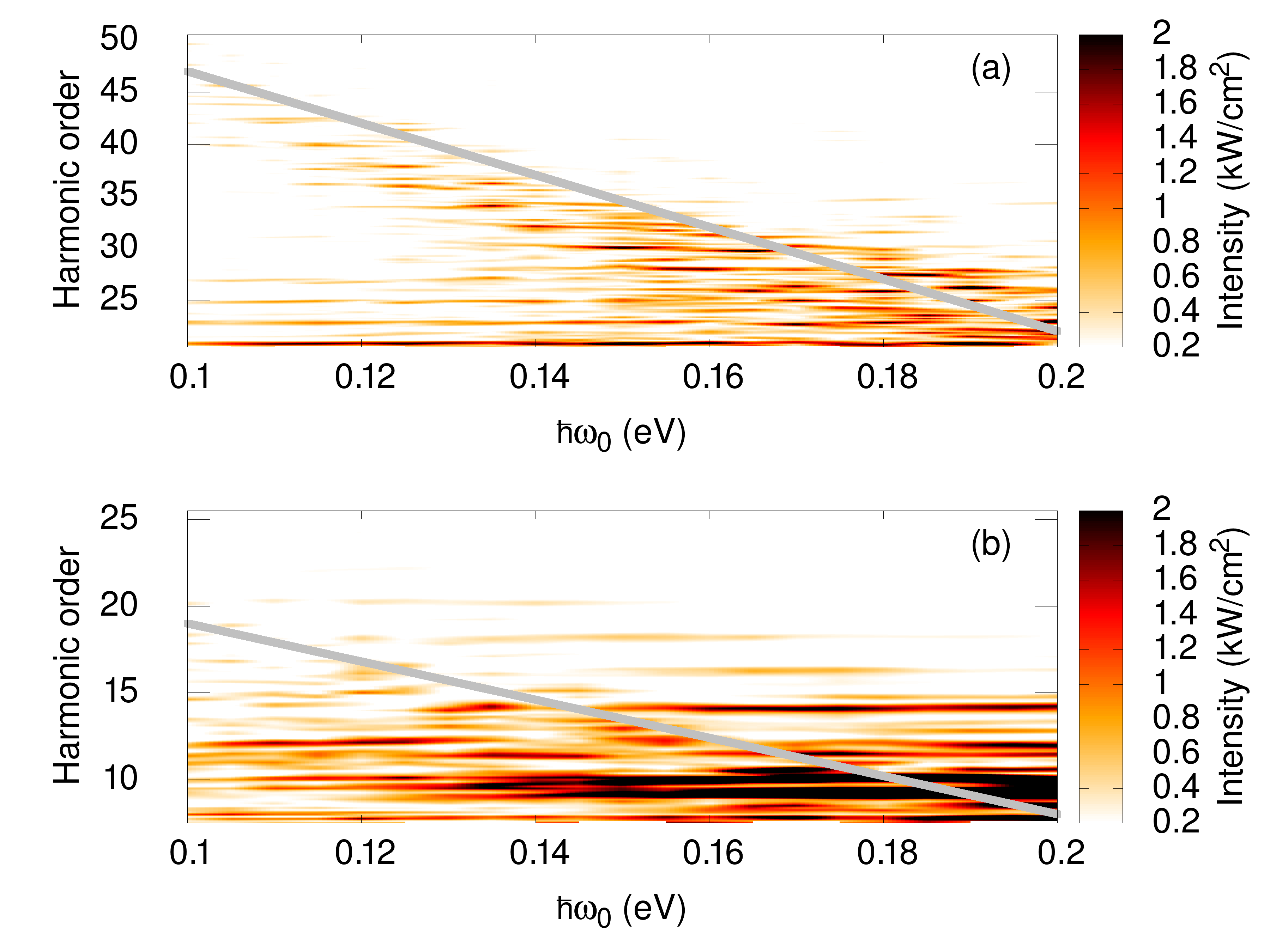
Figure 11: The intensity of HHG as a function of the fundamental frequency and the order of harmonics for graphene (a) and silicene (b) in the strong-field regime in the bichromatic driving field: $\omega_{0}^{\prime}=2\omega_{0}$, $\hat{\mathbf{e}}=\left\{1,0\right\}$, $\hat{\mathbf{e}}^{\prime}=\left\{0,1\right\}$, $\varphi=0$, and $\varepsilon=1$ The interaction parameter is $\chi_{0}=1.7$ and the relaxation time is taken to be $\Gamma^{-1}=40\ \mathrm{fs.}$ The grey straight lines in both cases are the saddle-point excitonic resonant photon energy.

The fingerprint of the saddle-point excitons is preserved also for the higher intensity of laser pulses. This is seen in Fig. 10, where we plotted the intensity of HHG as a function of the interaction parameter and harmonic’s photon energy for graphene and silicene. For comparison we also plotted the results obtained in the scope of FP model (a) and (c). Comparing the FP with HF approximation results we see that in the former case the slight enhancement of HHG intensity takes place near VHS $2\gamma_{0}$, while in the latter case the sharp enhancement for the wide rang of intensities takes place close to the saddle-point excitonic resonances. For graphene, this is $4-5.0\ \mathrm{eV}$ and for silicene $1.5-2.0\ \mathrm{eV}$. This tendency is also preserved for other frequencies of the driving field. In Fig. 11, the intensity of HHG as a function of the fundamental frequency and the order of harmonics for graphene and silicene in the bichromatic driving field is shown. On the same figure, we also plot the saddle-point excitonic resonant photon energy: the harmonic order for every driving fundamental frequency. As is seen, the sharp enhancement takes place along the excitonic resonances.

IV Conclusion

We have presented the microscopic theory of nonlinear interaction of a monolayer graphene/silicene with a strong infrared laser field near the VHS. We have numerically solved the Bloch equations within the Houston basis that takes into account the many-body Coulomb interaction in the HF approximation. As reference nanostructures, we have considered graphene and silicene. The obtained results show that saddle-point excitonic resonances have a significant impact on the HHG process in hexagonal 2D nanostructures. We have shown that in the bichromatic driving pulses that is composed of the fundamental wave of linear polarization and its second harmonic at the orthogonal polarization, one can effectively initiate spectral caustics in the HHG spectrum. In particular, we have shown that the plateau of the HHG spectrum has a peak near the harmonics close to SPER and redshifted from the VHS of the free-particle picture. The results of the current investigation are not only of theoretical/academic importance but also will have significant implications for the rapidly developing area of modern extreme nonlinear optics of nanostructures.

- [1] A. H. Castro Neto, F. Guinea, N. M. R. Peres, K. S. Novoselov, and A. K. Geim, Rev. Mod. Phys. 81, 109 (2009).
- [2] B. Lalmi, H. Oughaddou, H. Enriquez, A. Kara, S. Vizzini, B. Ealet, and B. Aufray, Applied Physics Letters 97, 223109 (2010).
- [3] P. Vogt, P. De Padova, C. Quaresima, J. Avila, E. Frantzeskakis, M.C. Asensio, A. Resta, B. Ealet and G. Le Lay, Phys. Rev. Lett. 108, 155501 (2012).
- [4] A. Fleurence, R. Friedlein, T. Ozaki, H. Kawai, Y. Wang, and Y. Yamada-Takamura, Phys. Rev. Lett. 108, 245501 (2012).
- [5] K. S. Novoselov, A. K. Geim, S. V. Morozov, D. Jiang, M. I. Katsnelson, I. V. Grigorieva, S. V. Dubonos, and A. A.Firsov, Nature 438, 197 (2005).
- [6] Y. B. Zhang, Y. W. Tan, H. L. Stormer, P. Kim, Nature 438, 201 (2005).
- [7] K. F. Mak, M. Y. Sfeir, Y. Wu, C. H. Lui, J. A. Misewich, and T. F. Heinz, Phys. Rev. Lett. 101, 196405 (2008).
- [8] T. Stauber, N. M. R. Peres, and A. K. Geim, Phys. Rev. B 78, 085432 (2008).
- [9] D. C. Elias, R. V. Gorbachev, A. S. Mayorov, S. V. Morozov, A. A. Zhukov, P. Blake, L. A. Ponomarenko, I. V. Grigorieva, K. S. Novoselov, F. Guinea, and A. K. Geim, Nat. Phys. 7, 701 (2011).
- [10] C. Hwang, D. A. Siegel, S. K. Mo, W. Regan, A. Ismach, Y. Zhang, A. Zettl, and A. Lanzara, Scientific Reports 2, 590 (2012).
- [11] C. H. Park, F. Giustino, C. D. Spataru, M. L. Cohen, and S. G. Louie, Nano Lett. 9, 4234 (2009).
- [12] K. I. Bolotin, F. Ghahari, M. D. Shulman, H. L. Stormer, and P. Kim, Nature 462, 196 (2009).
- [13] X. Du, I. Skachko, F. Duerr, A. Luican, & E. Y. Andrei, Nature 462, 192-195 (2009).
- [14] D. V. Khveshchenko, Phys. Rev. Lett. 87, 246802 (2001).
- [15] E. V. Gorbar, V. P. Gusynin, V. A. Miransky, and I. A. Shovkovy, Phys. Rev. B 66, 045108 (2002).
- [16] J. E. Drut and T. A. Lahde, Phys. Rev. Lett. 102, 026802 (2009).
- [17] E. H. Hwang and S. Das Sarma, Phys. Rev. B 75, 205418 (2007).
- [18] L. Yang, J. Deslippe, C. H. Park, M. L. Cohen, and S. G. Louie, Phys. Rev. Lett. 103, 186802 (2009).
- [19] V. G. Kravets, A. N. Grigorenko, R. R. Nair, P. Blake, S. Anissimova, K. S. Novoselov, and A. K. Geim, Phys. Rev. B 81, 155413 (2010).
- [20] K. F. Mak, J. Shan, & T. F. Heinz, Phys. Rev. Lett. 106, 046401 (2011).
- [21] K. F. Mak, F. H. da Jornada, K. He, J. Deslippe, N. Petrone, J. Hone, J. Shan, S. G. Louie, and T. F. Heinz, Phys. Rev. Lett. 112, 207401 (2014).
- [22] N. M. R. Peres, R. M. Ribeiro, & A. H. Castro Neto, Phys. Rev. Lett. 105, 055501 (2010)
- [23] E. G. Mishchenko, Phys. Rev. Lett. 98, 216801 (2007).
- [24] H. Rezania, Z. Aghai Manesh, Physica E 56, 32 (2014).
- [25] L. B. Drissi, F. Z. Ramadan, Physica E 68, 38 (2015).
- [26] V. Apinyan, T.K. Kopeć, Physica E 122, 114145 (2020).
- [27] L. Van Hove, Phys. Rev. 89, 189 (1953).
- [28] M. Breusing, S. Kuehn, T. Winzer, E. Malic, F. Milde, N. Severin, J.P. Rabe, C. Ropers, A. Knorr, T. Elsaesser, Phys. Rev. B 83, 153410 (2011).
- [29] E. Malic, T. Winzer, E. Bobkin, A. Knorr, Phys. Rev. B 84, 205406 (2011).
- [30] E. Malic, A. Knorr, Graphene and carbon nanotubes: ultrafast optics and relaxation dynamics. John Wiley & Sons, (2013).
- [31] B. Y. Sun, Y. Zhou, and M. W. Wu, Phys. Rev. B 85, 125413 (2012).
- [32] Z. Sun, D. N. Basov, and M. M. Fogler, Phys. Rev. B 97, 075432 (2018).
- [33] J. L. Cheng, J. E. Sipe, and C. Guo, Phys. Rev. B 100, 245433 (2019).
- [34] H. Rostami, E. Cappelluti, npj 2D Materials and Applications 5, 1 (2021).
- [35] H. K. Avetissian, Relativistic Nonlinear Electrodynamics: The QED Vacuum and Matter in Super-Strong Radiation Fields (Springer, Berlin 2015).
- [36] S. A. Mikhailov, Physica E 40, 2626 (2008); S. A. Mikhailov, K. Ziegler, J. Phys. Condens. Matter 20, 384204 (2008).
- [37] H. K. Avetissian, A. K. Avetissian, G. F. Mkrtchian, Kh. V. Sedrakian, Phys. Rev. B 85, 115443 (2012).
- [38] P. Bowlan, E. Martinez-Moreno, K. Reimann, T. Elsaesser, and M. Woerner, Phys. Rev. B 89, 041408(R) (2014).
- [39] I. Al-Naib, J. E. Sipe, and M. M. Dignam, Phys. Rev. B 90, 245423 (2014); I. Al-Naib, J. E. Sipe, and M. M. Dignam, New J. Phys. 17, 113018 (2015).
- [40] L. A. Chizhova, F. Libisch, and J. Burgdorfer, Phys. Rev. B 94, 075412 (2016).
- [41] H. K. Avetissian, G. F. Mkrtchian, Phys. Rev. B 94, 045419 (2016).
- [42] L. A. Chizhova, F. Libisch, and J. Burgdorfer, Phys. Rev. B 95, 085436 (2017).
- [43] H. K. Avetissian, G. F. Mkrtchian, Phys. Rev. B 97, 115454 (2018).
- [44] Ó. Zurrón, A. Picón, and L. Plaja, New J. Phys. 20, 053033 (2018).
- [45] H. K. Avetissian, G. F. Mkrtchian, K. G. Batrakov, S. A. Maksimenko, A. Hoffmann, Phys. Rev. B 88, 165411 (2013).
- [46] M. Du, C. Liu, Z. Zeng, R. Li, Phys. Rev. A 104, 033113 (2021).
- [47] M. S. Mrudul and G. Dixit, Phys. Rev. B 103, 094308 (2021).
- [48] D. Dimitrovski, L. B. Madsen, and T. G. Pedersen, Phys. Rev. B 95, 035405 (2017).
- [49] H. K. Avetissian, G. F. Mkrtchian, Phys. Rev. B 99, 085432 (2019).
- [50] N. Yoshikawa, T. Tamaya, and K. Tanaka, Science 356, 736 (2017).
- [51] C. Liu, Y. Zheng, Z. Zeng, R. Li, Phys. Rev. A 97, 063412 (2018).
- [52] Ó. Zurrón-Cifuentes, R. Boyero-García, C. Hernández-García, A. Picón, L. Plaja, Optics express 27, 7776 (2019).
- [53] F. Dong, Q. Xia, J. Liu, Phys. Rev. A 104, 033119 (2021).
- [54] S. A. Sato, H. Hirori, Y. Sanari, Y. Kanemitsu, and A. Rubio, Phys. Rev. B 103, L041408 (2021).
- [55] Y. Zhang, L. Li, J. Li, T. Huang, P. Lan, P. Lu, Phys. Rev. A 104, 033110 (2021).
- [56] X. Q. Wang, X. B. Bian, Phys. Rev. A 103 053106 (2021).
- [57] Y. Feng, S. Shi, J. Li, Y. Ren, X. Zhang, J. Chen, H. Du, Phys. Rev. A 104 043525 (2021).
- [58] H. K. Avetissian, G. F. Mkrtchian, A. Knorr, Phys. Rev. B 105, 195405 (2022).
- [59] K. S. Budil, P. Salières, A. L’Huillier, T. Ditmire, and M. D. Perry, Phys. Rev. A 48, R3437 (1993).
- [60] M. Lewenstein, P. Balcou, M. Y. Ivanov, A. L’Huillier, and P. B. Corkum, Phys. Rev. A 49, 2117 (1994).
- [61] G. Vampa, C. R. McDonald, G. Orlando, D. D. Klug, P. B. Corkum and T. Brabec, Phys. Rev. Lett. 113, 073901 (2014).
- [62] G. Vampa and T. Brabec, J. Phys. B: At. Mol. Opt. Phys. 50, 083001 (2017).
- [63] H. K. Avetissian, A. K. Avetissian, B. R. Avchyan, and G. F. Mkrtchian, Phys. Rev. B 100, 035434 (2019).
- [64] L. Yue and M. B. Gaarde, Phys. Rev. A 103, 063105 (2021).
- [65] A. J. Uzan, G. Orenstein, Á. Jiménez-Galán, C. McDonald, R. E. F. Silva, B. D. Bruner, N. D. Klimkin, V. Blanchet, T. Arusi-Parpar, M. Krüger, A. N. Rubtsov, O. Smirnova, M. Ivanov, B. Yan, T. Brabec, and N. Dudovich, Nat. Photonics 14, 183 (2020).
- [66] A.D. Güclü, P. Potasz, M.Korkusinski, and P. Hawrylak, Graphene Quantum Dots (Springer, 2014).
- [67] M. Polini, A. Tomadin, R. Asgari, A. H. MacDonald, Phys. Rev. B 78, 115426 (2008).
- [68] J. C. Phillips, Phys. Rev. 136, A1705 (1964).
- [69] B. Velický and J. Sak, Phys. Status Solidi 16, 147 (1966).
- [70] E. O. Kane, Phys. Rev. 180, 852 (1969).
- [71] I. Balslev, Solid State Commun. 52, 351 (1984).
- [72] P. Y. Yu and M. Cardona, Fundamentals of semiconductors: Physics and materials properties (Springer, Berlin, 1996).
- [73] U. Fano, Phys. Rev. 124, 1866 (1961).
- [74] D.-H. Chae, T. Utikal, S. Weisenburger, H. Giessen, K. v. Klitzing, M. Lippitz, and J. Smet, Nano Letters 11, 1379 (2011).