Thermalization of locally perturbed many-body quantum systems

Abstract

Deriving conditions under which a macroscopic system thermalizes directly from the underlying quantum many-body dynamics of its microscopic constituents is a long-standing challenge in theoretical physics. The well-known eigenstate thermalization hypothesis (ETH) is presumed to be a key mechanism, but has defied rigorous verification for generic systems thus far. A weaker variant (weak ETH), by contrast, is provably true for a large variety of systems, including even many integrable models, but its implications with respect to the problem of thermalization are still largely unexplored. Here we analytically demonstrate that systems satisfying the weak ETH exhibit thermalization for two very natural classes of far-from-equilibrium initial conditions: the overwhelming majority of all pure states with a preset non-equilibrium expectation value of some given local observable, and the Gibbs states of a Hamiltonian which subsequently is subject to a quantum quench in the form of a sudden change of some local system properties.

I Introduction

Statistical mechanics for systems at thermal equilibrium is a highly developed cornerstone of theoretical physics. Its universal and in principle surprisingly simple “working recipe” is to properly choose and evaluate one of the textbook canonical ensembles. Even though the considered systems may be out of equilibrium at the beginning, these concepts are meant to apply to all sufficiently late times, i.e., after the initial relaxation processes have died out. While this prediction or postulate of thermalization is known to be extremely successful in practice, a direct derivation from the basic laws of physics is widely considered as a very important and still not satisfactorily solved problem.

The most common and natural starting point in this context is to focus on isolated quantum many-body systems, with the objective to explain why they generically exhibit thermalization in the long run, i.e., why they are very well described – after the relaxation of the possibly far-from-equilibrium initial state has been completed – by a microcanonical ensemble (or by an equivalent canonical ensemble), as predicted by the textbooks. Indeed, this has been the main goal in most of the pioneering works in this field [1, 2, 3, 4]. A key role in this context is played by the so-called eigenstate thermalization hypothesis (ETH) [1, 2, 5, 6]. Specifically, the best-known or “strong” version of the ETH (sETH) can be readily shown to guarantee thermalization under rather mild and physically reasonable preconditions on the considered observables and initial states [7, 8, 9, 10, 11]. The sETH itself, however, still amounts to an unproven hypothesis, and is actually known to be violated by integrable, many-body localized, and even certain non-integrable models [7, 8, 9, 10, 11]. Accordingly, to analytically deduce thermalization directly from the unitary quantum dynamics remains one of the main challenges in this research area.

On the other hand, a weaker version of the ETH (wETH) has recently been analytically established for a large variety of systems [12, 13, 14, 11, 15, 16], but its implications with respect to the issue of thermalization are still not very well understood. This is the main objective of our present paper: Focusing on cases where the wETH is known to apply, we will identify two very large and natural classes of non-equilibrium initial states for which thermalization can be analytically verified, namely typical pure states with tunable (non-equilibrium) expectation values of local observables in Sec. III and local quenches from thermal equilibrium (Gibbs) states in Sec. IV. Notably, while the sETH mainly concerns so-called non-integrable systems, the wETH and thus our present results also pertain to many integrable models.

II Preliminaries

II.1 Setup

As announced, we consider isolated quantum system with $L\gg 1$ degrees of freedom, which are moreover known to satisfy the wETH. We thus focus on translationally invariant spin models with short range interactions, periodic boundary conditions, and for simplicity we restrict ourselves to one-dimensional lattices with sites $i=1,...,L$ (various generalizations are straightforward, see also Sec. V below). Accordingly, the Hamiltonian is of the form

$$H=\sum_{i=1}^{L}h_{i}\ ,$$ (1)

where the $h_{i}$ are translational copies of the same local (few-body and short-range) operator, meaning that every $h_{i}$ only acts nontrivially on lattice sites sufficiently close to $i$. The eigenvalues of $H$ are denoted by $E_{n}$, the eigenvectors by $|n\rangle$, and the underlying Hilbert space by ${\cal H}$, where $n=1,...,N$ and $N$ is exponentially large in the system size $L$. Furthermore, we mainly have in mind observables $O$ which are local operators as specified above (and are thus sometimes written in the form $O_{i}$), or suitable sums thereof, as exemplified by the energy (1). Focusing on such observables is very common and generally considered to still cover most situations of actual interest [7, 8, 9, 10, 11].

As detailed in [12, 13, 14, 11, 15, 16], these Hamiltonians and observables can be shown to satisfy the wETH, meaning that the empirical variance of the diagonal matrix elements $O_{nn}:=\langle n\rvert O\lvert n\rangle$ taken over macroscopically small energy intervals vanishes in the thermodynamic limit $L\to\infty$ [see also Eq. (3) below].

II.2 Typical equilibrium states, clustering, and weak ETH

Our first objective is to demonstrate thermalization for a large class of non-equilibrium initial states. Similarly as in the well-known previous explorations of (canonical) typicality and concentration of measure phenomena [17, 18, 19], we therefore focus on a microcanonical energy window ${\cal I}_{\mathrm{mc}}:=[E-\Delta,E]$, and we denote by $S$ the concomitant subset of indices $n$ with $E_{n}\in{\cal I}_{\mathrm{mc}}$, by $P:=\sum_{n\in S}|n\rangle\langle n|$ the projector onto the so-called energy shell (sub-Hilbert space) $\hat{\cal H}$, and by $|S|:=\mbox{Tr}\{P\}$ its dimension. Furthermore, the energy interval ${\cal I}_{\mathrm{mc}}$ can and will be chosen large on microscopic and small on macroscopic scales, i.e., $|S|$ is still exponential in the system size $L$, while any (normalized) state $|\psi\rangle\in\hat{\cal H}$ exhibits a macroscopically well-defined energy (small energy spread). According to textbook statistical mechanics, the expectation value of an observable $O$ at thermal equilibrium then follows as $\mbox{Tr}\{\rho_{\mathrm{mc}}O\}$, where $\rho_{\mathrm{mc}}:=P/|S|$ is the microcanonical ensemble. Observing that all normalized $|\psi\rangle\in\hat{\cal H}$ are of the form $\sum_{n\in S}c_{n}|n\rangle$ with $c_{n}\in{\mathbb{C}}$ and $\sum_{n\in S}|c_{n}|^{2}=1$, we may view them as points on the unit sphere in ${\mathbb{C}}^{|S|}$ (or ${\mathbb{R}}^{2|S|}$). If one samples states uniformly from that sphere, it has been shown for instance in Refs. [17, 18, 19] that they typically amount to equilibrium states in the sense that the expectation values $\langle O\rangle_{\!\psi}:=\langle\psi|O|\psi\rangle$ are very close to the thermal equilibrium value $\langle O\rangle_{\!\mathrm{mc}}:=\mbox{Tr}\{\rho_{\mathrm{mc}}O\}$ for the overwhelming majority of all those $|\psi\rangle$. More precisely speaking, the difference $\langle O\rangle_{\!\psi}-\langle O\rangle_{\!\mathrm{mc}}$ is exponentially small in $L$ apart from an exponentially small fraction of exceptional $|\psi\rangle$’s.

Importantly, the operator $O$ in the above typicality result may actually be chosen largely arbitrarily (it may be non-local and even non-Hermitian). One thus can conclude that, for instance, also the correlations

$$C_{\!\psi}(O_{i},O_{j}^{\prime}):=\langle O_{i}O_{j}^{\prime}\rangle_{\!\psi}-\langle O_{i}\rangle_{\!\psi}\langle O_{j}^{\prime}\rangle_{\!\psi}$$ (2)

between two local observables $O_{i}$ and $O^{\prime}_{j}$ will be exponentially close to $C_{\!\mathrm{mc}}(O_{i},O_{j}^{\prime}):=\langle O_{i}O_{j}^{\prime}\rangle_{\!\mathrm{mc}}-\langle O_{i}\rangle_{\!\mathrm{mc}}\langle O_{j}^{\prime}\rangle_{\!\mathrm{mc}}$ for the vast majority of all $|\psi\rangle$’s.

Our first remark is that the general mindset of such a typicality approach is very natural from the common information-theoretic viewpoint in statistical physics: Since the actual system state in a real experiment is usually not exactly known (and in fact not even reproducible), it is sensible to randomly sample states $|\psi\rangle$ which conform with the available information (here the pertinent energy interval ${\cal I}_{\mathrm{mc}}$) but are otherwise as unbiased as possible. The above typicality result guarantees that practically all those random states then indeed behave almost identically (as expected in the real experiment). The generalization when additional information about the initial state is available will be addressed in the next section.

Our second remark is that, according to common (textbook) wisdom, the standard thermal equilibrium ensembles do not exhibit any unphysical properties. It follows that the same must apply to the overwhelming majority of the $|\psi\rangle$’s since they behave practically indistingushable from a microcanonical ensemble.

Nevertheless, it might a priori not be immediately obvious, for example, whether our simple-minded random states $|\psi\rangle$ satisfy the so-called cluster decomposition property (CDP), which requires that the correlations (2) must decay to zero with increasingly large distance between the lattice sites $i$ and $j$ [6, 20, 21, 22, 23, 24, 25, 26]. Indeed, following Weinberg [27], the CDP is by now a well-established premise which any physically realistic state is supposed to fulfill (at least outside the realm where phase transitions may occur). The justification is considered as essentially self-evident: Physically realistic states of macroscopic systems, as we consider them here, are not expected to admit correlations between local properties with large spatial separation. To formally verify the CDP itself for a given (pure or mixed) state is in general a quite difficult task. However, in our present case we can exploit that the CDP has been established in [28, 29, 30, 31, 32] for thermal Gibbs states (canonical ensembles), and that the equivalence of ensembles has been shown in [33] to apply even for non-local observables of the form $O_{i}O_{j}^{\prime}$. We thus can conclude that the CDP is also satisfied by our microcanonical ensemble $\rho_{\mathrm{mc}}$, and finally, according to the argument below (2), also by the overwhelming majority of the pure states $|\psi\rangle$.

Note that the above quoted proofs of the CDP and the equivalence of ensembles [28, 29, 30, 31, 32, 33] only apply to short-ranged Hamiltonians. Likewise, our states $\lvert\psi\rangle$ are sampled from a subspace (energy shell) which itself encapsulates substantial information about the underlying Hamiltonian’s “locality” properties. By contrast, when sampling random $|\psi\rangle$’s from a high-dimensional but otherwise arbitrary subspace of ${\cal H}$, the majority of them may well violate the CDP in general.

Our last remark is that we now have all the necessary ingredients at hand to formally state the wETH: Recalling that $O_{nn}:=\langle n\rvert O\lvert n\rangle$, it essentially requires that

$$\Delta_{O}^{\,2}:=\frac{1}{\lvert S\rvert}\sum_{n\in S}\big{(}O_{nn}-\langle O\rangle_{\!\mathrm{mc}}\big{)}^{\!2}\to 0\ \mbox{ for}\ L\to\infty$$ (3)

if one adopts the usual (physically natural) scaling of the microcanonical energy window ${\cal I}_{\mathrm{mc}}$ with the system size $L$ [12, 13, 14, 11, 15, 16].

III Thermalization and clustering for typical non-equilibrium initial states

III.1 Result

To arrive at our first main result, we consider a particularly simple and natural extension of the above specified typicality approach into the non-equilibrium realm. Namely, let us assume that, besides the pertinent energy interval ${\cal I}_{\mathrm{mc}}$, also the (possibly far from equilibrium) expectation value of some specific local observable $A$ is (approximately) known, e.g., because it has been tuned experimentally to prepare the system out of equilibrium. Accordingly, among all the $\lvert\psi\rangle$’s from before, we only keep a subset of states which comply with this extra information that $\langle A\rangle_{\!\psi}$ is close to some given non-equilibrium value $a$. The ensemble of all these states thus gives rise to a statistical operator $\rho$ which is still reminiscent of a microcanonical ensemble, albeit with the additional constraint $\mbox{Tr}\{\rho A\}\simeq a$ (akin to a “generalized microcanonical ensemble” [34]). In particular, we still expect the CDP to hold, see also the discussion around Fig. 2 below. To explicitly construct those random states $|\psi\rangle$ and the concomitant ensemble $\rho$, we adopted the previously developed formalism from Refs. [35, 36], see also Sec. III.3 for further details.

The first main result of our present paper is that when considering such $|\psi\rangle$’s as initial states, which subsequently evolve in time according to $|\psi(t)\rangle=e^{-iHt}|\psi\rangle$, then the overwhelming majority of them exhibits thermalization. More precisely, the time-dependent expectation values $\langle O\rangle_{\!\psi(t)}:=\langle\psi(t)|O|\psi(t)\rangle$ of an observable $O$, which may but need not be equal to $A$, stay close to the thermal equilibrium value $\langle O\rangle_{\!\mathrm{mc}}$ for nearly all sufficiently late times $t$. (In particular, not only long-time averages but single time points are thus considered.) As usual [9, 10, 11], some non-small deviations $\langle O\rangle_{\!\psi(t)}-\langle O\rangle_{\!\mathrm{mc}}$ may still occur during the initial relaxation process and also at certain arbitrarily late but very rare times $t$ (quantum revivals). Quantitatively, the deviations $\langle O\rangle_{\!\psi(t)}-\langle O\rangle_{\!\mathrm{mc}}$ are predicted to decrease as $L^{-1/2}$ for the vast majority of all (sufficiently late) times $t$ and initial states $|\psi\rangle$, the exceptional $t$’s and $|\psi\rangle$’s being exponentially rare in $L$. The derivation will be given in Sec. III.3 below.

III.2 Example

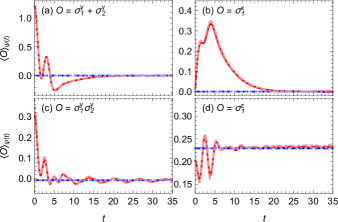
Figure 1: Numerical illustration of thermalization for the integrable model (4) with $L=28$, $J=\frac{1}{2}$, and $g=\frac{1}{4}\,$. Red solid: Expectation values $\langle O\rangle_{\!\psi(t)}$ of various observables $O$ (see legend; note the different $y$-axis scales). Blue dashed: Thermal expectation values of $O$. Red dash-dotted and blue dotted: Same for $L=24$ (sometimes hardly distinguishable from $L=28$). As detailed in the main text, the initial states $|\psi\rangle$ and the thermal expectation values were obtained by utilizing a Gaussian filter with parameters $\gamma=2.5/L$, $\lambda=-0.35\,L$ (the ground state energy is close to $-0.53\,L$), and by imposing the non-equilibrium initial value $\langle A\rangle_{\!\psi}\simeq 1.2$ for the observable $A=\sigma^{y}_{1}+\sigma^{y}_{2}$ ($=O$ from (a)).

A numerical illustration of our analytical result is provided in Fig. 1 for the common transverse-field Ising model (TFIM) [9, 21, 37] with

$$H = -J\,\sum_{i=1}^{L}\sigma^{x}_{i}\sigma^{x}_{i+1}-g\sum_{i=1}^{L}\sigma^{z}_{i},$$ (4)

where the Pauli matrices $\sigma_{i}^{\nu}$ with $\nu\in\{x,y,z\}$ and $\sigma^{\nu}_{i\pm L}:=\sigma^{\nu}_{i}$ (periodic boundary conditions) describe the spin components at the chain site $i\in\{1,...,L\}$. This model obeys the wETH, but violates the sETH, and is integrable in the sense that there exists an extensive number of local integrals of motion (conserved quantities) $I_{k}$ which commute with $H$ and with each other. Explicitly, the $I_{k}$ with odd and even $k\geq 1$ are given by [9, 21]

$$I_{2j-1} = -J\,\sum_{i=1}^{L}(\tau^{xx}_{i,j+1}+\tau^{yy}_{i,j-1})+g\,\sum_{i=1}^{L}(\tau^{xx}_{i,j}+\tau^{yy}_{i,j}),$$

$$I_{2j} = -J\,\sum_{i=1}^{L}(\tau^{xy}_{i,j}-\tau^{yx}_{i,j})\ ,$$ (5)

where $\tau^{\nu\mu}_{i,l\geq 1}:=\sigma_{i}^{\nu}\sigma_{i+1}^{z}\cdots\sigma_{i+l-1}^{z}\sigma_{i+l}^{\mu}$ and $\tau^{\nu\mu}_{i,0}:=-\sigma_{i}^{z}$.

To construct the states $\lvert\psi\rangle$, and also to determine $\langle O\rangle_{\!\mathrm{mc}}$, the projector $P$ onto the energy shell is needed, which requires the eigenvalues and eigenvectors of the Hamiltonian $H$. While these can be explicitly obtained for the present system in principle [37], storing enough of them to reach a sensible size of the energy shell is beyond our computational resources for the rather large systems in Fig. 1. We therefore followed Ref. [38] (and further references cited therein) to approximate $P$ by a so-called Gaussian filter $P_{\!g}:=\exp\{-\gamma(H-\lambda)^{2}\}$, and analogously for $\langle O\rangle_{\!\mathrm{mc}}$, see also Appendix B for additional numerical details. Once a non-equilibrium initial state $|\psi\rangle$ has been found, we numerically determined its time evolution by means of Suzuki-Trotter product expansion techniques [39]. Likewise, $P_{\!g}$ from above was numerically obtained via imaginary time evolution.

The examples in Fig. 1 nicely confirm our general analytical prediction of thermalization. We also verified (not shown) that the results for different randomly sampled initial states $|\psi\rangle$ are nearly indistinguishable (as predicted above Eq. (8)). Moreover, the example in Fig. 1 illustrates that, indeed, thermalization may even occur in integrable systems with far-from-equilibrium initial conditions.

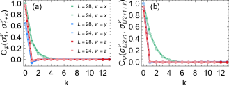
Figure 2: Correlation $C_{\psi}(\sigma^{\nu}_{j},\sigma^{\nu}_{j+k})$ from (2) between local spin operators (Pauli matrices $\sigma_{i}^{\nu}$) as a function of their spatial separation $k$, for the same model Hamiltonian (4) and initial states $\lvert\psi\rangle$ as in Fig. 1. (a) $j=1$, i.e., the first observable $\sigma^{\nu}_{j}$ appearing in $C_{\psi}(\sigma^{\nu}_{j},\sigma^{\nu}_{j+k})$ is located at one of the sites which are also affected by the observable $A=\sigma^{y}_{1}+\sigma^{y}_{2}$ that governs the initial non-equilibrium constraint. (b) $j=L/2+1$, i.e., the first observable $\sigma^{\nu}_{j}$ appearing in $C_{\psi}(\sigma^{\nu}_{j},\sigma^{\nu}_{j+k})$ is located “far away from $A$”.

Finally, one may wonder, similarly as in the previous section, whether the states $|\psi\rangle$ still satisfy (with overwhelming probability) the CDP in spite of the additional constraint that $\langle A\rangle_{\!\psi}$ must now be close $a$ (see Sec. III.1). Analogously to the unconstrained case, the above mentioned dynamical typicality framework [35, 36] now readily implies that this is equivalent to the question whether the concomitant ensemble $\rho$ exhibits the CDP. Since analytical results regarding the CDP are still rather scarce and the few existing proofs rather involved, and since this question is not really a central issue of our present work, we content ourselves with a numerical illustration, shown in Fig. 2 for the same setting as in Fig. 1: Both in the vicinity of the “perturbation” $A$ (left panel, $j=1$) and far away from it (right panel, $j=\frac{L}{2}+1$), the correlations $C_{\psi}(\sigma^{\nu}_{j},\sigma^{\nu}_{j+k})$ decay to zero with increasing separation $k$ between the observables’ supports. Similarly as in Fig. 1, dynamical typicality furthermore predicts, and our numerical results (not shown) confirm, that also practically any other initial state $\lvert\psi\rangle$ generated in this way exhibits practically the same behavior of $C_{\psi}(\sigma^{\nu}_{j},\sigma^{\nu}_{j+k})$ as in Fig. 2. Altogether, the numerics thus provides strong evidence that the CDP is still fulfilled for the vast majority of our non-equilibrium initial states $|\psi\rangle$.

III.3 Derivation

Turning to the derivation of thermalization for most pure states from the above introduced ensemble of $\lvert\psi\rangle$’s, our starting point is the so-called dynamical typicality framework by Bartsch and Gemmer [35], see also Refs. [40, 36]. Concretely, the $\lvert\psi\rangle$’s are constructed as

$$|\psi\rangle:={\cal{N}}\,Q\sum_{n=1}^{N}z_{n}\,|n\rangle\,,$$ (6)

where $|n\rangle$ are the energy eigenstates (or any other orthonormal basis of ${\cal H}$) and $z_{n}$ are complex numbers, whose real and imaginary parts are given by independent, Gaussian distributed random variables of zero mean and unit variance. Moreover,

$$Q:=P+yPAP$$ (7)

and ${\cal{N}}$ is a normalization constant so that $\langle\psi|\psi\rangle=1$. It follows that $|\psi\rangle\in\hat{\cal H}$, and that the ensemble of random states considered in Sec. II.2 is recovered in the special case $y=0$. Following [35], the purpose of the extra parameter $y$ is to account for the additional condition that $\langle A\rangle_{\!\psi}$ must be with high probability close to a fixed value $a$, see also Eq. (14) below. The statistical operator $\rho$ associated with this ensemble and introduced in Sec. III.1 is thus $\rho:=[\,|\psi\rangle\langle\psi|\,]_{z}$ where the symbol $[\,\cdot\,]_{z}$ indicates the average over all the Gaussian random numbers $z_{n}$ from above.

Dynamical typicality [35, 40, 36] then asserts that, for any given $t\geq 0$, the time-evolved expectation values $\langle O\rangle_{\!\psi(t)}$ for nearly all those $\lvert\psi\rangle$’s practically coincide with those obtained from the time evolution $\rho(t):=e^{-iHt}\rho e^{iHt}$ of $\rho$, provided that $\rho$ itself is of low purity, i.e., $\mbox{Tr}\{\rho^{2}\}\ll 1$. As a second ingredient, we invoke the well-established fact [8, 9, 10, 11] that the long-time average of the expectation value $\mbox{Tr}\{\rho(t)O\}$ can be written in the form $\mbox{Tr}\{\bar{\rho}\,O\}:=\sum_{n\in S}\rho_{nn}O_{nn}$, where $\bar{\rho}$ denotes the so-called diagonal ensemble (in case of degeneracies, the eigenstates $|n\rangle$ must be chosen so that $O$ is diagonal in the corresponding eigenspaces of $H$). Furthermore, it has been demonstrated, e.g., in Refs. [41] that the time dependent expectation values $\mbox{Tr}\{\rho(t)O\}$ remain very close to the time-average $\mbox{Tr}\{\bar{\rho}\,O\}$ for the vast majority of all sufficiently late times $t$ under quite weak conditions: Essentially, it is sufficient that the energy differences $E_{m}-E_{n}$ do not coincide for too many index pairs with $m\not=n$, which is the case for any generic Hamiltonian $H$ [4, 42, 41], and that $\mbox{Tr}\{\bar{\rho}^{2}\}\ll 1$, which in turn is guaranteed under the same condition $\mbox{Tr}\{\rho^{2}\}\ll 1$ as before [36]. To finally establish thermalization, one has to show that $\mbox{Tr}\{\bar{\rho}O\}$ practically coincides with $\langle O\rangle_{\!\mathrm{mc}}$. We achieve this by rewriting the difference $\overline{\Delta O}:=\mbox{Tr}\{\bar{\rho}O\}-\langle O\rangle_{\!\mathrm{mc}}$ as $\sum_{n\in S}\rho_{nn}(O_{nn}-\langle O\rangle_{\!\mathrm{mc}})$ and then exploiting the Cauchy-Schwarz inequality to obtain

$$\overline{\Delta O}^{2} \leq \Delta_{O}^{\,2}\,|S|\sum_{n\in S}(\rho_{nn})^{2}\ ,$$ (8)

where $\Delta_{O}^{\,2}$ is the wETH characteristic from (3). Furthermore, we can upper bound the sum in (8) by $\sum_{m,n=1}^{N}|\rho_{mn}|^{2}=\mbox{Tr}\{\rho^{2}\}$, yielding

$$\overline{\Delta O}^{\,2}\leq\Delta_{O}^{\,2}\,\lvert S\rvert\,\mbox{Tr}\{\rho^{2}\}\ .$$ (9)

Since we focus on systems for which the wETH is fulfilled, the quantity $\Delta_{O}^{\,2}$ approaches zero for large $L$ according to (3).

The remaining task is to establish an $L$-independent upper bound for the quantity $|S|\mbox{Tr}\{\rho^{2}\}$ appearing on the right hand side of (9) and to show that, as a consequence, $\mbox{Tr}\{\rho^{2}\}\ll 1$ for asymptotically large $L$ as required twice above (8).

Obviously, the operator $PAP=:\hat{A}_{r}$ in (7) is the projection/restriction of the original observable $A$ to the energy shell $\hat{\cal H}$ (hence the “hat” symbol). Possibly after adding a trivial constant to the observable $A$, and then multiplying it by a constant factor, we can assume without loss of generality that $\hat{A}_{r}$ has been “rescaled” (hence the index “$r$”) so that $\mbox{Tr}\{\rho_{\mathrm{mc}}\hat{A}_{r}\}=0$ and $\mbox{Tr}\{\rho_{\mathrm{mc}}\hat{A}_{r}^{2}\}=1$ [35]. Finally, the eigenvalues of $\hat{A}_{r}$ are denoted as $a_{n}$ and the $k$-th moment of the eigenvalue distribution as

$$m_{k}:=\frac{1}{|S|}\sum_{n\in S}(a_{n})^{k}=\frac{1}{|S|}\mbox{Tr}\{\hat{A}_{r}^{k}\}=\mbox{Tr}\{\rho_{\mathrm{mc}}\hat{A}_{r}^{k}\}\ .\ \$$ (10)

The above mentioned rescaling thus implies $m_{1}=0$ and $m_{2}=1$, and $Q$ from (7) can be rewritten as $P+y\hat{A}_{r}$.

One of the main results obtained in [36] is that $\rho$ can be approximated arbitrarily well by $\tilde{\rho}:=Q^{2}/\mbox{Tr}\{Q^{2}\}$ provided $\mbox{Tr}\{\tilde{\rho}^{2}\}$ is sufficiently small. In the following, we therefore tacitly replace $\tilde{\rho}$ by $\rho$ and subsequently verify that $\mbox{Tr}\{\rho^{2}\}\ll 1$. By means of a straightforward but somewhat tedious calculation (working in the eigenbasis of $\hat{A}_{r}$) one thus can infer that

$$\rho=\frac{1}{|S|}\frac{1}{1+y^{2}}(P+y\hat{A}_{r})^{2}\ .$$ (11)

Moreover, the expectation value of $\hat{A}_{r}$ is found to be

$$\mbox{Tr}\{\rho\hat{A}_{r}\}=\frac{2y+m_{3}y^{2}}{1+y^{2}}\ ,$$ (12)

and for the purity of $\rho$ one obtains

$$\mbox{Tr}\{\rho^{2}\}=\frac{1}{|S|}\frac{1+6y^{2}+4m_{3}y^{3}+m_{4}y^{4}}{(1+y^{2})^{2}}\ .$$ (13)

Generally speaking, the eigenvalues and eigenvectors of the restricted and rescaled operator $\hat{A}_{r}$ have little to do with those of the original observable $A$. Yet it seems reasonable to expect that the eigenvalue distribution of $\hat{A}_{r}$ does not exhibit long tails so that, given its first two moments are $m_{1}=0$ and $m_{2}=1$, also the next two moments $m_{3}$ and $m_{4}$ will be (at most) on the order of unity, see also [43] for a numerical example. We thus can conclude that by choosing suitable parameter values $y$, expectation values in (12) of up to the order of unity (in modulus) can be generated [35]. Furthermore, the purity in (13) is (for any $y$) on the order of $1/|S|$, which in turn is exponentially small in the system size $L$ (see Sec. II.2).

Altogether, we can conclude that $|S|\mbox{Tr}\{\rho^{2}\}$ is upper bounded by an $L$-independent constant and that $\mbox{Tr}\{\rho^{2}\}$ is exponentially small in $L$, which completes our demonstration of thermalization. For the remaining quantitative details mentioned at the end of Sec. III.1, namely the precise scaling of the fraction of exceptional $\lvert\psi\rangle$’s and the deviations $\left\langle O\right\rangle_{\!\psi(t)}-\langle O\rangle_{\!\mathrm{mc}}$, we refer to Appendix A.

We close with two side remarks: First, one may wonder why only local observables $A$ are admitted in Ref. [35] and in the above considerations. In fact, one can show that $A$ may actually also consist of any linear combination of local operators, as long as the number of summands remains small. On the other hand, if $A$ is, for example, an extensive observable, as exemplified by the energy in (1), then notable deviations of $\langle A\rangle_{\!\psi}$ from the thermal equilibrium value $\langle A\rangle_{\!\mathrm{mc}}$ can no longer be achieved by means of our present general framework for the following reason: By exploiting (12) and the dynamical typicality formalism from Refs. [36], one can show that the expectation value $\left\langle A\right\rangle_{\!\psi}$ of the original observable $A$ is exponentially likely to be exponentially close to

$$\mbox{Tr}\{\rho A\}=\langle A\rangle_{\!\mathrm{mc}}+s\,\frac{2y+m_{3}y^{2}}{1+y^{2}}\ ,$$ (14)

where $0\leq s\leq\sqrt{\mbox{Tr}\{\rho_{\mathrm{mc}}(A-\langle A\rangle_{\!\mathrm{mc}})^{2}\}}$ (thermal fluctuations of $A$). As a consequence, the typical relative deviations of $\left\langle A\right\rangle_{\!\psi}$ from the thermal equilibrium value $\langle A\rangle_{\!\mathrm{mc}}$ must remain very small if $A$ is an extensive observable.

Second, the above mentioned exponentially likely proximity of $\left\langle A\right\rangle_{\!\psi}$ to $\mbox{Tr}\{\rho A\}$ does not yet exclude the existence of a very unlikely subset of $|\psi\rangle$’s with substantial deviations of $\langle A\rangle_{\!\psi}$ from $\mbox{Tr}\{\rho A\}$. On the other hand, one readily verifies that this exceptional subset can be excluded from the total set of admitted $|\psi\rangle$’s right from the beginning, entailing only exponentially small corrections in all the subsequent calculations. This extra step has been tacitly taken for granted at the beginning of the Sec. III.1.

IV Thermalization of a quenched Gibbs state

IV.1 Result

We now turn to the second main result of our paper: Let us assume that the initial state is given by a thermal Gibbs state (canonical ensemble) of the form

$$\rho:=Z_{0}^{-1}e^{-\beta H_{0}}\ ,\ \ Z_{0}:=\mbox{Tr}\{e^{-\beta H_{0}}\}\ ,$$ (15)

where $H_{0}$ is different from the Hamiltonian $H$ in (1) which governs the subsequent temporal evolution. (Note that the restrictions on $H$, such as translational invariance, do not apply to $H_{0}$.) In other words, the system is in thermal equilibrium for $t<0$ and is subject to an instantaneous “quantum quench” at $t=0$, with pre-quench Hamiltonian $H_{0}$ and post-quench Hamiltonian $H$. Moreover, we focus on so-called local quenches, meaning that the difference $V:=H-H_{0}$ between the post- and pre-quench Hamiltonians is a local operator. Note that, despite their apparent “smallness” (compared to $H_{0}$ and $H$), it has been observed numerically in a somewhat different context that such local perturbations of $H_{0}$ can still have profound effects, for instance changing a system violating the sETH into one satisfying it [44, 45, 46]. Likewise, such local quenches may still give rise to far-from-equilibrium initial expectation values (see Fig. 3(a)).

From a different standpoint, since the change of the Hamiltonian is restricted to a finite subsystem, the situation immediately after the quench may also be viewed as a “small” non-equilibrium system in contact with a “large” thermal bath. Although it may seem intuitively reasonable to expect thermalization for such a setup, verifying this by analytical means is nevertheless an important and challenging problem, whose solution is the second main achievement of our present paper.

Namely, assuming again that $H$ obeys the wETH (3), we can demonstrate that the time-evolved expectation values $\mbox{Tr}\{\rho(t)O\}$, where $\rho(t):=e^{-iHt}\rho\,e^{iHt}$ with $\rho$ from (15), are practically indistinguishable from $\langle O\rangle_{\!\mathrm{mc}}:=\mbox{Tr}\{\rho_{\mathrm{mc}}O\}$ for nearly all sufficiently late times $t$, where $\rho_{\mathrm{mc}}$ is the microcanonical post-quench ensemble with appropriate energy $\mbox{Tr}\{\rho_{\mathrm{mc}}H\}=\mbox{Tr}\{\rho H\}$. This result will be derived in Sec. IV.3 below.

IV.2 Example

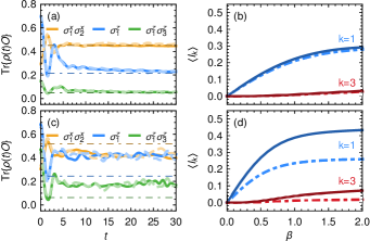
Figure 3: Thermalization (top) and non-thermalization (bottom) after a canonical quench. The post-quench Hamiltonian $H$ is given by the integrable model (4) with $J=\frac{1}{2}$ and $g=\frac{1}{4}$. The pre-quench Hamiltonian $H_{0}$ is given by $H-\frac{3}{4}(\sigma^{z}_{1}+\sigma^{z}_{2})$ in the top panels (local quench such that the total transverse field is $g=1$ for the first two sites, but $g=\frac{1}{4}$ for all other sites), and by $H$ from (4) with $J=\frac{1}{2}$ and $g=1$ in the bottom panels (global quench). In both cases, a canonical initial state $\rho:=e^{-\beta H_{0}}/\mbox{Tr}\{e^{-\beta H_{0}}\}$ (see (15)) was numerically explored by utilizing dynamical typicality [36] and Suzuki-Trotter product expansion techniques [39], while $\rho^{\prime}:=e^{-\beta^{\prime}\!H}/\mbox{Tr}\{e^{-\beta^{\prime}\!H}\}$ with $\beta^{\prime}$ so that $\mbox{Tr}\{\rho^{\prime}H\}=\mbox{Tr}\{\rho H\}$ was used as thermal reference ensemble, see also main text. (a,c): Time-dependent expectation values of three observables (see legend) for $\beta=1$. Solid: $L=24$; dashed: $L=20$; dash-dotted: thermal values $\mbox{Tr}\{\rho^{\prime}O\}$ (indistinguishable for $L=24$ and $L=20$). (b,d): Conserved quantities $I_{k}$ from (5) for $k=1,3$ versus $\beta$. [Graphs for even $k$ are very close to zero and therefore not shown.] Solid: conserved expectation values $\mbox{Tr}\{\rho(t)I_{k}\}=\mbox{Tr}\{\rho I_{k}\}$. Dash-dotted: thermal values $\mbox{Tr}\{\rho^{\prime}I_{k}\}$. The system size is $L=24$ (data for $L=20$ would be indistinguishable on the given scale).

Our analytical prediction of thermalization after local quenches is exemplified by Fig. 3(a,b) for the TFIM from (4). In particular, these numerical findings illustrate that even integrable systems may thermalize after a local quench. (For numerical convenience, we actually employed not the microcanonical but the equivalent canonical ensemble [15, 16, 47, 48, 33, 49, 50, 51] to evaluate the thermal expectation values, see also the discussion below Eq. (5)). Moreover, Fig. 3(a) shows that local observables may initially still exhibit far-from-equilibrium expectation values, whereas the conserved quantities in Fig. 3(b) indeed assume the pertinent (time-independent) thermal values, as it must be. Remarkably, the results in Fig. 3(a,b) are (nearly) $L$-independent, i.e., the large-$L$ asymptotics can be anticipated without a sophisticated finite size analysis.

For comparison, Fig. 3(c,d) also illustrates the effects of a global quench, resembling those of a local quench for short times, but exhibiting non-thermalization in the long run, as expected for the integrable post-quench Hamiltonian $H$ at hand (similar examples can also be found in Refs. [49, 50, 51]).

With regard to related previous works we remark that thermalization might also be inferred from Refs. [24, 25, 26] for the example from Fig. 3(a,b), since this specific post-quench Hamiltonian $H$ amounts to a so-called non-interacting integrable model. Furthermore, as far as $\beta$-values below $0.386$ are concerned, thermalization might be understood by combining the findings from Ref. [22] with those of Ref. [31] (and some additional calculations which we omit). By contrast, our present analytical result is not restricted to non-interacting integrable models or small $\beta$-values. Finally, the first steps of our derivation (see below) are also somewhat reminiscent of Theorem 3 in [20], Sec. 6 in [13], Sec. 6 in [7], or Theorem 1 in [52], but not the more demanding subsequent steps (beginning with Eq. (25), in particular).

IV.3 Derivation

The first tasks in our derivation of thermalization after local quenches are exactly as in Sec. III.3, except that $\rho$ is now given by (15): We have to show that $\mbox{Tr}\{\rho^{2}\}\ll 1$ and that $\overline{\Delta O}:=\mbox{Tr}\{\bar{\rho}O\}-\langle O\rangle_{\!\mathrm{mc}}$ is negligibly small. Recalling that the textbook free energy $F_{\beta}$ associated with the Gibbs ensemble (15) obeys the relation $e^{-\beta F_{\beta}}=\mbox{Tr}\{e^{-\beta H_{0}}\}$, one can conclude that $\mbox{Tr}\{\rho^{2}\}=e^{-2\beta\Delta_{\beta}}$ with $\Delta_{\beta}:=F_{2\beta}-F_{\beta}$. Taking for granted that the system exhibits generic thermodynamic properties [7], it follows that $\Delta_{\beta}$ is an extensive quantity, hence $\mbox{Tr}\{\rho^{2}\}$ decreases exponentially with $L$. Turning to $\overline{\Delta O}$, one readily sees, similarly as in Sec. III.3, that

$$\overline{\Delta O} = X_{1}+X_{2}\ ,$$ (16)

$$X_{1} := \sum_{n=1}^{N}\rho_{nn}(O_{nn}-\langle O\rangle_{\!\mathrm{mc}}^{\prime})\ ,$$ (17)

$$X_{2} := \langle O\rangle_{\!\mathrm{mc}}^{\prime}-\langle O\rangle_{\!\mathrm{mc}}\ ,$$ (18)

where $\langle O\rangle_{\!\mathrm{mc}}^{\prime}:=\mbox{Tr}\{\rho_{\mathrm{mc}}^{\prime}O\}$ and $\rho_{\mathrm{mc}}^{\prime}$ is the microcanonical ensemble that reproduces the energy of the post-quench canonical ensemble $\rho_{\mathrm{th}}$ given by

$$\rho_{\mathrm{th}} := Z^{-1}\,e^{-\beta H}=\sum_{n=1}^{N}p_{n}\lvert n\rangle\langle n\rvert\ ,$$ (19)

$$p_{n} := Z^{-1}\,e^{-\beta E_{n}}\ ,$$ (20)

$$Z := \mbox{Tr}\{e^{-\beta H}\}=\sum_{n=1}^{N}e^{-\beta E_{n}}\ ,$$ (21)

i.e., $\mbox{Tr}\{\rho_{\mathrm{mc}}^{\prime}H\}=\mbox{Tr}\{\rho_{\mathrm{th}}H\}$. Given that $H$ and $H_{0}$ only differ by a local operator (see above), it is reasonable to expect that the relative difference between the two energies $\mbox{Tr}\{\rho_{\mathrm{th}}H\}$ and $\mbox{Tr}\{\rho H_{0}\}$ approaches zero for large $L$, and likewise for the concomitant difference in (18). The quite arduous analytical confirmation of this expectation can be found in Appendix C.

The remaining task is to upper bound $X_{1}$ in (17). To this end, we split each summand in (17) into a factor $\rho_{nn}/p_{n}^{1/2}$ and a factor $p_{n}^{1/2}(O_{nn}-\langle O\rangle_{\!\mathrm{mc}}^{\prime})$, and then invoke the Cauchy-Schwartz inequality to conclude that

$$X_{1}^{2} \leq c^{\prime}\Delta_{O}^{\prime\,2}\ ,$$ (22)

$$c^{\prime} := \sum_{n=1}^{N}(\rho_{nn})^{2}/p_{n}\ ,$$ (23)

$$\Delta_{O}^{\prime\,2} := \sum_{n=1}^{N}p_{n}\big{(}O_{nn}-\langle O\rangle_{\!\mathrm{mc}}\big{)}^{\!2}\ .$$ (24)

One readily recognizes quite considerable similarities to the discussion around (8): First, $\Delta_{O}^{\prime\,2}$ obviously amounts to the canonical counterpart of the corresponding microcanonical quantity $\Delta_{O}^{\,2}$ from (3). Second, since we focus on systems for which the wETH is fulfilled, we thus can again conclude that $\Delta_{O}^{\prime\,2}$ approaches zero for large $L$, see also Appendix B.3 for more details. Finally, we are again left to show that $c^{\prime}$ (which is obviously the canonical counterpart of $|S|\sum_{n\in S}(\rho_{nn})^{2}$ in (8)) remains bounded for large $L$.

To do so, we start by considering the operator-valued function

$$\Phi(\lambda):=e^{\lambda H/2}\,e^{-\lambda H_{0}}\,e^{\lambda H/2}\ .$$ (25)

One readily verifies that $\Phi(\lambda)$ is Hermitian and that the derivative $\Phi^{\prime}(\lambda):=d\Phi(\lambda)/d\lambda$ can be written as

$$\Phi^{\prime}(\lambda) = e^{\lambda H/2}\frac{H-H_{0}}{2}e^{-\lambda H_{0}}e^{\lambda H/2}$$ (26)

$$+ e^{\lambda H/2}e^{-\lambda H_{0}}\frac{H-H_{0}}{2}e^{\lambda H/2}\ .$$

Exploiting (25), $V:=H-H_{0}$, and

$$V_{\lambda}:=e^{-\lambda H/2}\,V\,e^{\lambda H/2}\,,$$ (27)

we thus arrive at

$$\Phi^{\prime}(\lambda) = \frac{V_{\lambda}^{\dagger}\Phi(\lambda)+\Phi(\lambda)V_{\lambda}}{2}\ .$$ (28)

Rewriting (15) with (25) as

$$\rho=Z_{0}^{-1}e^{-\beta H/2}\,\Phi(\beta)\,e^{-\beta H/2}$$ (29)

and recalling that $|n\rangle$ and $E_{n}$ are the eigenvectors and eigenvalues of $H$, it follows that

$$\langle n|\rho|n\rangle=Z_{0}^{-1}e^{-\beta E_{n}}\,\langle n|\Phi(\beta)|n\rangle\ .$$ (30)

With (20) we thus can rewrite (23) as

$$c^{\prime} = \sum_{n=1}^{N}\frac{Z^{2}}{Z_{0}^{2}}\,p_{n}\,\langle n|\Phi(\beta)|n\rangle^{2}$$ (31)

$$\leq \frac{Z^{2}}{Z_{0}^{2}}\max_{n}\langle n|\Phi(\beta)|n\rangle^{2}\sum_{n=1}^{N}p_{n}$$

$$= \frac{Z^{2}}{Z_{0}^{2}}\max_{n}\langle n|\Phi(\beta)|n\rangle^{2}\ .$$

To proceed, we utilize that $H$ in (1) is a sum of local operators $h_{i}$, whose operator norms $\|h_{i}\|$ can be bounded from above by an $i$- and $L$-independent constant. Denoting the support of $h_{i}$ (lattice sites on which $h_{i}$ acts nontrivially) by $\operatorname{supp}(h_{i})$, there must also exist an $L$-independent constant $R$ such that $\max\{\lvert x-y\rvert:x,y\in\operatorname{supp}(h_{i})\}\leq R$ for all $h_{i}$.

Next we observe that $V_{\lambda}$ from (27) can be understood as an imaginary-time evolution of the observable $V$ with the Hamiltonian $H$. Since $V$ is a local operator, its support $\operatorname{supp}(V)$ consists of a finite number of lattice sites $s_{V}:=\lvert\operatorname{supp}(V)\rvert$. For real-time evolution, it is well known that Lieb-Robinson bounds [53, 54] limit the growth of the support of the time-evolved observable $e^{iHt}Ve^{-iHt}$ with $t$ (up to exponentially decaying corrections). As far as our one-dimensional models (1) are concerned, similar bounds for the complex-time evolution as in (27) were first derived by Araki [28], with the difference that the “light cone” grows exponentially with the magnitude $\lvert\lambda\rvert$ of the complex time (as opposed to linear growth in Lieb-Robinson-type bounds). For our purposes, the following formulation based on Bouch [55] is particularly convenient: For fixed $\lambda$ and any integer $k>e^{c_{1}\lvert\lambda\rvert}$, we can decompose

$$V_{\lambda}=V_{\lambda}^{(k)}+\Delta_{\lambda}^{(k)}$$ (32)

such that $\operatorname{supp}(V_{\lambda}^{(k)})$ extends at most $k$ sites beyond $\operatorname{supp}(V)$ (meaning that for any $x\in\operatorname{supp}(V_{\lambda}^{(k)})$ there exists a $y\in\operatorname{supp}(V)$ with $\lvert x-y\rvert\leq k$) and

$$\|\Delta_{\lambda}^{(k)}\|\leq s_{V}\|V\|\,c_{2}\,e^{-k}\,,$$ (33)

where $c_{1},c_{2}>0$ are $L$-independent constants. Moreover, for sufficiently large $L>2(k-s_{V})$, $V_{\lambda}^{(k)}$ is independent of $L$. Consequently, $\|V_{\lambda}\|$ can be bounded from above by an $L$-independent constant. Since $V_{\lambda}$ is furthermore continuous in $\lambda$ (even as $L\to\infty$ [55]), there also exists a common, $L$-independent upper bound $M_{\beta}$ for all $\lambda\in[0,\beta]$, i.e.

$$\sup\{\|V_{\lambda}\|:\lambda\in[0,\beta]\}\leq M_{\beta}\,.$$ (34)

In addition, by the same arguments, also $\|V_{\lambda}^{\dagger}\|\leq M_{\beta}$ ($\lambda\in[0,\beta]$) for the same constant $M_{\beta}$. (Note that we can thus assume $\beta>0$ in the following without loss of generality because $V_{-\lambda}=V_{\lambda}^{\dagger}$. Moreover, a non-vanishing temperature $\beta^{-1}$ is tacitly taken for granted.)

Observing that $|\|B\|-\|C\||\leq\|B-C\|$ for arbitrary operators $B$, $C$, and choosing $B=\Phi(\lambda+d\lambda)$ and $C=\Phi(\lambda)$ it readily follows that

$$\left|\frac{d\,\|\Phi(\lambda)\|}{d\lambda}\right|\leq\|\Phi^{\prime}(\lambda)\|\ .$$ (35)

With (28) and (34) this implies

$$\left|\frac{d\,\|\Phi(\lambda)\|}{d\lambda}\right|\leq\|V_{\lambda}\|\|\Phi(\lambda)\|\leq M_{\beta}\|\Phi(\lambda)\|$$ (36)

for all $\lambda\in[0,\beta]$. Upon integrating this inequality and exploiting that $\|\Phi(0)\|=1$ according to (25), we finally obtain the $L$-independent upper bound

$$\|\Phi(\beta)\|\leq e^{\beta M_{\beta}}\ .$$ (37)

Since $|\langle n|\Phi(\beta)|n\rangle|\leq\|\Phi(\beta)\|$ for all $n$, we can infer from (31) and (37) that

$$c^{\prime} \leq \frac{Z^{2}}{Z_{0}^{2}}e^{2\beta M_{\beta}}\ .$$ (38)

Evaluating $Z_{0}$ in (15) by means of the basis $|n\rangle$, we obtain

$$Z_{0}=\sum_{n=1}^{N}\langle n|e^{-\beta H_{0}}|n\rangle=\sum_{n=1}^{N}Z_{0}\langle n|\rho|n\rangle\ .$$ (39)

Exploiting (30) on the right hand side of (39) implies

$$Z_{0}=\sum_{n=1}^{N}e^{-\beta E_{n}}\,\langle n|\Phi(\beta)|n\rangle\ ,$$ (40)

and similarly as in (31), (38) it follows with (21) that

$$Z_{0}\leq Z\,e^{\beta M_{\beta}}\ .$$ (41)

Upon exchanging the roles of $H_{0}$ and $H$, one analogously finds that

$$Z\leq Z_{0}\,e^{\beta M_{\beta}}\ .$$ (42)

With (38) we thus arrive at the $L$-independent upper bound

$$c^{\prime} \leq e^{4\beta M_{\beta}}\ .$$ (43)

V Discussion and conclusions

In conclusion, we analytically demonstrated thermalization for a large variety of non-equilibrium initial conditions with local perturbation traits, including the overwhelming majority of initial states with a preset expectation value of some local observable and initial Gibbs states after a local quantum quench. For instance, this may describe a small subsystem far from equilibrium in contact with a thermal bath (rest of the system). Besides focusing – as usual – on local observables (and suitable sums thereof), the (post-quench) Hamiltonian is required to obey the wETH, which has been proven, among others, for many very common translationally invariant models with short-range interactions [12, 13, 14, 11, 15, 16]. In particular, non-integrable as well as integrable models are admitted. As an example, we numerically illustrated our prediction of thermalization for the integrable TFIM (4), and also the previously known absence of thermalization after a global quench.

Moreover, these many-body initial states were demonstrated to obey the cluster decomposition property, i.e., they are not marred by unphysical “non-locality” features in the form of correlations over large distances.

To keep things simple, we focused on one-dimensional models and employed the language of spin models, but fermionic systems or particle-number-conserving bosonic systems can be readily transformed into spin models preserving the local structure (in one dimension) and are thus equally covered. In higher dimensions, generally speaking, additional complications like phase transitions will unavoidably occur at least for some members of the admitted model class. As a consequence, already the wETH itself, which we utilized as an ingredient in our present approach, is only known to be true for energies sufficiently far above the realm where such systems in principle may exhibit a phase transition [12, 13, 14, 11, 15, 16]. Similar restrictions apply to the known proofs of the cluster decomposition property for thermal Gibbs states [28, 29, 30, 31, 32], which served as another ingredient of our present explorations. Nevertheless, provided that those two preconditions are met, our results regarding thermalization and clustering for typical non-equilibrium pure states can be readily adapted as well. In turn, the imaginary-time analogs of the Lieb-Robinson bounds, which we employed in our analysis of the initial Gibbs states, are until now not available in higher dimensions. Altogether, developing a common framework for thermalization and phase transitions thus remains as a very challenging task for future research.

Finally, we point out that the wETH is essential in those findings in the sense that systems violating it (e.g., many-body-localized ones) can generally not be expected to thermalize from similar initial conditions.

To conclude, the ubiquity of thermalization is a very well established empirical observation in numerical and real-world experiments, and has the status of an axiom in textbook (equilibrium) statistical mechanics. Our present results may be considered as a notable step forward in the long-standing but still largely unsolved task to theoretically explain this empirical observation directly from the underlying microscopic dynamics.

Appendix A Typicality, equilibration, and thermalization

In this appendix, we provide the quantitative details regarding thermalization of typical pure states. We heavily draw on previously established analytical results in the context of “dynamical typicality”. In doing so, we mainly employ the most general version of this formalism from Ref. [36], which unifies and extends a considerable number of important precursory works (see references therein).

Following Ref. [36], our starting point is an $N$-dimensional Hilbert space ${\cal H}$, spanned by some orthonormal basis $\{|\chi_{n}\rangle\}_{n=1}^{N}$. For instance, the $|\chi_{n}\rangle$ may be the eigenvectors of some Hamiltonian $H$. In any case (see also main text), we focus on many-body systems with a large but finite number $L$ of degrees of freedom, and the Hilbert space dimension $N$ is understood to be exponentially large in $L$ but finite. Generalizations to infinite $N$ are straightforward [36], but omitted here in order to avoid inessential technicalities.

A.1 Dynamical typicality

As in Sec. III.3, we define an ensemble of normalized random vectors $|\psi\rangle\in{\cal H}$ via

$$|\psi\rangle={\cal{N}}\,Q\sum_{n=1}^{N}z_{n}\,|\chi_{n}\rangle\ ,$$ (44)

where the $z_{n}$ are complex numbers, whose real and imaginary parts are given by independent, Gaussian distributed random variables of zero mean and unit variance. Moreover, $Q$ is a linear operator on ${\cal H}$, which for the moment may still be (practically) arbitrary (in particular, $Q$ need not be Hermitian); for the ensemble under study in the main text, e.g., we have

$$Q=P+yPAP\,,$$ (45)

cf. Eq. (7). Finally, ${\cal{N}}$ is a normalization constant so that $\langle\psi|\psi\rangle=1$.

A key property of the random vector ensemble in (44) is its invariance under arbitrary unitary transformations of the basis $|\chi_{n}\rangle$ of ${\cal H}$ (all statistical properties remain unchanged). In other words, the basis can be chosen arbitrarily. This is of particular interest when numerically sampling random vectors according to (44), since any single-particle product basis will do the job. In our numerical explorations, we always employed such a “computational basis” $|\chi_{n}\rangle$.

Given some (non-zero) $Q$, one readily verifies that

$$\rho:=Q\,Q^{\dagger}/\mbox{Tr}\{Q\,Q^{\dagger}\}\ .$$ (46)

is Hermitian, positive semidefinite, and of unit trace, i.e., a well-defined density operator. While $Q$ was until now (practically) arbitrary, we henceforth restrict ourselves to $Q$’s so that $\rho$ in (46) amounts to a mixed state of small purity, i.e., we require that

$$\mbox{Tr}\{\rho^{2}\}\ll 1\ .$$ (47)

(See also Sec. III.3, where Eq. (47) was established for the ensemble (46) with $Q$ from (45).)

Incidentally, a convenient way to numerically check (47) is as follows: Similarly as before, we sample random vectors $|\psi\rangle$ according to (44), however we do not normalize them but rather set ${\cal{N}}=1$ in (44). Hence, the quantity $x:=\langle\psi|\psi\rangle$ is now a random variable. Likewise, when independently sampling two random vectors, say $|\phi\rangle$ and $|\psi\rangle$, according to (44) with ${\cal{N}}=1$, the quantity $y:=|\langle\phi|\psi\rangle|^{2}$ will be another random variable. Denoting by ${\mathbb{E}}[x]$ and ${\mathbb{E}}[y]$ the expectation values of $x$ and $y$, one readily finds by means of the general framework from Ref. [36] that $\mbox{Tr}\{\rho^{2}\}={\mathbb{E}}[y]/({\mathbb{E}}[x])^{2}$. Under the assumption that the probability distributions of both random variables $x$ and $y$ are reasonably well-behaved, a decent order-of-magnitude estimate of their expectation values and of $\mbox{Tr}\{\rho^{2}\}$ can thus be obtained by means of only a quite small number of random vectors.

Next we consider, as in the main text, the pure states $|\psi\rangle$ from (44) as initial conditions at time $t=0$, which then evolve according to the Schrödinger equation $i\,\mbox{d}|\psi(t)\rangle/\mbox{d}t=H|\psi(t)\rangle$, implying $|\psi(t)\rangle=U_{t}|\psi\rangle$ with $U_{t}:=e^{-iHt}$, and resulting in expectation values $\langle O\rangle_{\!\psi(t)}:=\langle\psi(t)|O|\psi(t)\rangle$ for any given observable (Hermitian operator) $O$. Likewise, the initial state $\rho$ in (11) is governed by the von Neumann equation, implying $\rho(t):=U_{t}\rho U_{t}^{\dagger}$. Assuming that $\rho$ furthermore obeys (47), the main finding (for our purposes) from Ref. [36] then consist in the prediction that the approximation

$$\langle O\rangle_{\!\psi(t)}\simeq\mbox{Tr}\{\rho(t)O\}$$ (48)

will be fulfilled with very high accuracy for most normalized random vectors $|\psi\rangle$ in (44). A quantitative version of this prediction in terms of the small parameter $\epsilon:=(\mbox{Tr}\{\rho^{2}\})^{1/3}$ can be obtained along similar lines as in Sec. III.C of Ref. [56], resulting in

$${\cal P}\!\left(\,|\langle O\rangle_{\!\psi(t)}-\mbox{Tr}\{\rho(t)O\}|\geq\epsilon R_{\!\,O}\,\right)\leq 2\epsilon\ ,$$ (49)

where ${\cal P}(S)$ is the probability that the statement $S$ is true when randomly sampling an initial state $|\psi\rangle$ according to (44), and where $R_{\!\,O}$ is the measurement range (largest minus smallest eigenvalue) of the observable $O$. In the setting from the main text, the purity $\mbox{Tr}\{\rho^{2}\}$ is usually exponentially small in the system size $L$ (see Sec. III.3), hence also $\epsilon:=(\mbox{Tr}\{\rho^{2}\})^{1/3}$ in (49) is exponentially small in $L$.

Note that for any given $t$ there may still be a small probability to sample an “untypical” initial state $|\psi\rangle$, for which (48) is a bad approximation. Moreover, the set of all those untypical states may in general be different for different time points $t$. Likewise, for any given observable $O$, the set of untypical states $|\psi\rangle$ may in general be different. Finally, also the following generalized statement for any given observable $O$ can be readily shown along similar lines as in Sec. 17.4 of Ref. [57]: Apart from a set of untypical initial states $|\psi\rangle$, whose probability is exponentially small in $L$, the deviations in (48) are exponentially small in $L$ not only for an arbitrary but fixed time point $t$ (as predicted by (49)), but even simultaneously for the vast majority of all time points within any preset time interval $[t_{1},t_{2}]$, where the relative measure of exceptional time points is again exponentially small in $L$.

Apart from all those exponentially unlikely exceptions, the main implication of (48) is that initial states $|\psi\rangle$, randomly sampled according to (44), are very likely to exhibit very similar expectation values at the initial time $t=0$ and also at any later time $t>0$, a property which was originally discovered and named dynamical typicality in Ref. [35].

A.2 Equilibration and thermalization

Yet another relevant result from Ref. [36] is as follows: Similarly as in the main text, we say that the system exhibits equilibration if the expectation value $\langle O\rangle_{\!\psi(t)}$ remains very close to some constant “reference value” for the vast majority of all sufficiently large times $t$, i.e., after initial transients (relaxation processes) have died out. (We recall that a small fraction of exceptional, arbitrarily large times $t$ is unavoidable due to quantum revival effects.) On the other hand, the question of thermalization, i.e., whether or not this constant reference value is (nearly) equal to the pertinent thermal expectation value, is disregarded for the time being. According to (48), most initial states $|\psi\rangle$ will thus exhibit equilibration if the mixed state $\rho(t)$ exhibits equilibration. The latter has been demonstrated in Refs. [41] under quite weak conditions on the eigenvalues $E_{n}$ of $H$ and on the initial state $\rho(0)=\rho$: Essentially, it is sufficient that the energy differences $E_{m}-E_{n}$ do not coincide for too many index pairs with $m\not=n$ [which is the case for any generic Hamiltonian $H$ [42, 4, 41]], and that – in the absence of degeneracies – all eigenstates $|n\rangle$ of $H$ are weakly populated, i.e., $\langle n|\rho|n\rangle\ll 1$. As detailed in Ref. [36], the latter requirement is equivalent to $\sum_{n=1}^{N}(\langle n|\rho|n\rangle)^{2}\ll 1$, which in turn is once again guaranteed under the very same precondition as is (47). In case of degeneracies, a generalization along the lines of [41] is straightforward, but its detailed elaboration goes beyond our present scope.

Returning to the question of thermalization, and taking for granted the above mentioned conditions for equilibration, it is thus sufficient to show that the long-time average of the expectation value on the right hand side of (48) is well approximated by the corresponding thermal expectation value. In a first step, we therefore introduce $U_{t}:=e^{-iHt}$ and $\rho(t):=U_{t}\rho U_{t}^{\dagger}$ (see above (48)) on the right hand side of (48), and evaluate the trace in terms of the eigenvalues $E_{n}$ and eigenvectors $|n\rangle$ of $H$, yielding

$$\mbox{Tr}\{\rho(t)O\}=\sum_{m,n=1}^{N}\rho_{mn}\,O_{nm}\,e^{i(E_{n}-E_{m})t}$$ (50)

where $\rho_{mn}:=\langle m|\rho|n\rangle$ and $O_{nm}:=\langle n|O|m\rangle$. In case of degeneracies, we can and will choose the eigenvectors $|n\rangle$ so that $O$ is diagonal in the corresponding eigenspaces of $H$. Indicating the long-time average by an overline, we thus can conclude that

$$\overline{\mbox{Tr}\{\rho(t)O\}}=\sum_{n=1}^{N}\rho_{nn}\,O_{nn}=\mbox{Tr}\{\overline{\rho}\,O\}\ ,$$ (51)

where $\overline{\rho}$ is the so-called diagonal ensemble or long-time average of $\rho(t)$,

$$\overline{\rho}:=\sum_{N=1}^{N}\rho_{nn}\,|n\rangle\langle n|\ .$$ (52)

The remaining task is to show that the long-time average in (51) is (approximately) equal to the corresponding thermal equilibrium expectation value, which was accomplished in Sec. III.3.

Quantitatively, our conclusions are as follows: Given that the purity $\mbox{Tr}\{\rho^{2}\}$ is exponentially small in the system size (see Sec. III.3), the typical differences $\langle O\rangle_{\!\psi(t)}-\mbox{Tr}\{\rho(t)O\}$ were found, as detailed below (49), to be exponentially small in the system size $L$ for the vast majority of all (sufficiently late) times $t$, the exceptional $t$’s and $|\psi\rangle$’s being exponentially rare in $L$. Analogous conclusions can be shown [41] to apply to the differences $\mbox{Tr}\{\rho(t)O\}-\mbox{Tr}\{\overline{\rho}\,O\}$. Finally, the difference $\overline{\Delta O}:=\mbox{Tr}\{\bar{\rho}O\}-\langle O\rangle_{\!\mathrm{mc}}$ was found to obey $\overline{\Delta O}^{2}\leq c\Delta_{O}^{2}$ (see below Eq. (9)), where $c$ is a constant and $\Delta_{O}^{\,2}$ the wETH characteristic from (3). Quantitatively, pertinent previous investigations in Refs. [12, 58, 13, 14, 11, 59, 15, 16] suggest that $\Delta_{O}^{\,2}$ decreases (approximately) like $1/L$ with $L$. Altogether, $\langle O\rangle_{\!\psi(t)}-\langle O\rangle_{\!\mathrm{mc}}$ is thus predicted to decrease as $L^{-1/2}$ for the vast majority of all (sufficiently late) times $t$ and initial states $|\psi\rangle$, the exceptional $t$’s and $|\psi\rangle$’s being exponentially rare in $L$.

Appendix B Numerical implementation

Overall, (44) together with (45) amount to an explicit procedure of how to generate initial states $|\psi\rangle$ with a non-equilibrium expectation value of some given (local) observable $A$. The vast majority of those expectation values will be very close to the value on the right hand side of (14), which in turn can be adjusted by properly choosing the parameter $y$. A numerical implementation of this procedure is straightforward in principle (see also the discussion below (44)). In practice, the required projector $P$ onto the energy shell $\hat{\cal H}$ cannot be determined without diagonalizing the Hamiltonian $H$, thus limiting the numerics to relatively small systems. The main objective of this appendix is to circumvent such a diagonalization.

B.1 Setup

A well-established way to numerically overcome this problem [38] is to approximate the projector $P$ onto the energy shell $\hat{\cal H}$ by an “energy-filter” of the general form

$$P_{\nu}:=e^{-\gamma(H-\lambda)^{2\nu}}$$ (53)

with $\nu\in{\mathbb{N}}$ and suitably chosen parameters $\gamma$ and $\lambda$. Indeed, for sufficiently large $\nu$ and appropriate values of $\gamma$ and $\lambda$, the effect of $P_{\nu}$ approximates that of $P$ arbitrarily well for any eigenvector $|n\rangle$ of $H$ and thus for any $|\phi\rangle\in{\cal H}$. Similarly, one may expect that $\nu=1$ still amounts to an acceptable compromise between a reasonable approximation of $P$ and numerical feasibility [38]. From now on, we thus restrict ourselves to such “Gaussian energy filters” (hence the subscript “$g$”) of the form

$$P_{\!g}:=e^{-\gamma(H-\lambda)^{2}}\ .$$ (54)

As said in the main text, our actual numerical implementation of how the operator $P_{\!g}$ acts on any given state $|\phi\rangle\in{\cal H}$ is based on imaginary time evolution methods in combination with Suzuki-Trotter product expansion techniques [39].

Since the fundamental property $P^{2}=P$ of a genuine projector is no longer rigorously satisfied by $P_{\!g}$ from (54), the appropriate way of how to replace $P$ by $P_{\!g}$ in (45) is not immediately obvious. For instance, (45) is equivalent to $Q=P(1+yA)P$, but when replacing $P$ by $P_{\!g}$, two different descendants of the two originally identical $Q$’s are obtained. To us, the most natural modification of (45) seems to be

$$Q=P_{\!g}(1+yA)P_{\!g}\ .$$ (55)

It should be emphasized that in the end it will turn out not to be very important how closely (54) and (55) approximate their original counterparts (and likewise for similar further approximations later on). The reason is that we finally will obtain a new (numerical) way in its own right of how to generate initial states $|\psi\rangle$ which exhibit non-equilibrium expectation values of $A$ and thermalization in the long run.

Given (55), the sampling of random states $|\psi\rangle$ and the density operator $\rho$ are again determined by (44) and (46), the condition (47) can again be numerically examined as described below (47), and also the subsequent steps (48)-(52) remain valid.

Practically, results for many different parameter values $y$ in (55) can be conveniently produced in one numerical run as follows. The basic idea is to divide (44) into several substeps by numerically generating the (not normalized) random vectors (see also discussion below (44))

$$|\phi\rangle := \sum_{n=1}^{N}z_{n}\,|\chi_{n}\rangle\ ,$$ (56)

$$|\psi_{1}\rangle := P_{g}^{2}|\phi\rangle\ ,$$ (57)

$$|\psi_{2}\rangle := P_{g}AP_{\!g}|\phi\rangle\ .$$ (58)

The normalized vector $|\psi\rangle$ in (44) with $Q$ from (55) is thus recovered via

$$|\psi\rangle := {\cal{N}}(|\psi_{1}\rangle+y|\psi_{2}\rangle)\ .$$ (59)

However, instead of time evolving $|\psi\rangle$ and then evaluating the expectation values of some observables of interest, one can also time evolve $|\psi_{1}\rangle$ and $|\psi_{2}\rangle$ separately, and only then evaluate the expectation values, and analogously for the estimate of $\mbox{Tr}\{\rho^{2}\}$ described below (47). For instance, to determine the normalization constant ${\cal N}$ for arbitrary $y$ values, one only needs the three ($y$-independent) quantities $\langle\psi_{1}|\psi_{1}\rangle$, $\langle\psi_{1}|\psi_{2}\rangle$, and $\langle\psi_{2}|\psi_{2}\rangle$, and analogously for any expectation value. In particular, one can thus numerically adapt $y$ so that the initial expectation value of $A$ assumes some preset value (provided it can be realized at all by some value of $y$), and one can evaluate the behavior of several different such initial values in one numerical run.

The next problem is how to appropriately define the thermal equilibrium expectation value of $O$, with which the long-time average in (51) must be compared in order to decide whether or not thermalization takes place. The usual and natural solution is to choose once again some suitable energy window ${\cal I}_{\mathrm{mc}}:=[E-\Delta,E]$ so that the corresponding microcanonical ensemble $\rho_{\mathrm{mc}}$ (see also main text) imitates the energy distribution of the actual $\rho$ in (46) as closely as possible. More precisely, $E$ and $\Delta$ must be chosen so that the mean and variance of the energy distributions agree, i.e., $\mbox{Tr}\{\rho_{\mathrm{mc}}H\}=\mbox{Tr}\{\rho H\}$ and $\mbox{Tr}\{\rho_{\mathrm{mc}}H^{2}\}=\mbox{Tr}\{\rho H^{2}\}$ (note that $\mbox{Tr}\{\rho H^{k}\}=\mbox{Tr}\{\rho(t)H^{k}\}=\mbox{Tr}\{\overline{\rho}H^{k}\}$ for any $k\in{\mathbb{N}}$ according to (50) and (51)). However, to determine such an ensemble $\rho_{\mathrm{mc}}$ is again numerically inconvenient for the same reasons as those mentioned at the beginning of this section.

The solution of this problem is based on the fact that a so-called equivalence-of-ensembles property has been derived in Refs. [16, 33, 48] basically under the same preconditions as those which are required in the proofs of the wETH, and which we thus tacitly take for granted anyway (see also main text). Essentially, this means that the above specified microcanonical ensemble $\rho_{\mathrm{mc}}$ can be replaced by other ensembles of the general “diagonal form” (52), provided that the level populations $\rho_{nn}$ depend sufficiently smoothly on the energies $E_{n}$, and, as before, the mean and variance of the energy distribution are close to those of the actual ensemble from (46).

Obviously, a natural candidate of this kind is obtained by setting $y=0$ in (55) and then evaluating (46). Indeed, similarly as observed around Eq. (14) in the main text, it turns out that only local observables $A$ are of actual interest, for which the mean and variance of the energy distribution hardly change with $y$ in (55). Altogether, it is thus justified to approximate the thermal equilibrium expectation $\langle O\rangle_{\!\mathrm{mc}}:=\mbox{Tr}\{\rho_{\mathrm{mc}}O\}$ by

$$\langle O\rangle_{\!\mathrm{mc}}=\mbox{Tr}\{\rho_{\mathrm{th}}O\}\ ,$$ (60)

where the “thermal reference ensemble” (index “th”) is defined as

$$\rho_{\mathrm{th}}:=(P_{\!g})^{4}/\mbox{Tr}\{(P_{\!g})^{4}\}\ .$$ (61)

see also Appendix C below. Note that the above mentioned equivalence of ensembles and the concomitant approximation (60) are predicted to become exact for asymptotically large systems, while for finite systems it is reasonable to expect that the remaining difference between long-time average and thermal value will usually be even smaller when employing the auxiliary thermal ensemble $\rho_{\mathrm{th}}$ from (61) instead of its microcanonical counterpart $\rho_{\mathrm{mc}}$.

Numerically, the expectation value on the right hand side of (60) can once again be readily approximated by choosing $y=0$ in the procedure described below (59).

Note that all traces of an energy interval (or energy shell) have now disappeared. Hence the basic requirement that all considered states $|\psi\rangle$ must exhibit a narrow energy distribution (see main text) has now to be (numerically) verified by choosing $y=0$ and evaluating the variance $\langle H^{2}\rangle_{\psi}-\langle H\rangle_{\psi}^{2}$ along the lines described below (59).

In this context it is also noteworthy that the mean and variance of the energy distribution for the ensemble in (61) are only well approximated by $\lambda$ and $1/8\gamma$ according to (54) under the condition that the level density of $H$ can be considered as approximately constant within a neighborhood of $\lambda$ on the order of $\gamma^{-1/2}$. Otherwise, the relation of the parameters $\lambda$ and $\gamma$ to the mean and variance of the energy distribution is non-trivial and must be determined numerically.

B.2 Dynamical typicality

Following Appendix A, dynamical typicality for the present $\rho$ from (46) with $Q$ from (55) (and $y\neq 0$) is established if we can show $\mbox{Tr}\{\rho^{2}\}$ to be small, cf. Eq. (47). This can be achieved by a tedious, but straightforward calculation, whose steps parallel those described in the main text, see Sec. III.3. It results in the bound

$$\mbox{Tr}\{\rho^{2}\}\leq p_{\mathrm{max}}\,\frac{1+6y^{2}+4m_{3}y^{3}+m_{4}y^{4}}{(1+\tilde{m}_{2}y^{2})^{2}}\,,$$ (62)

where $m_{k}:=\mbox{Tr}\{\rho_{\mathrm{th}}A^{k}_{r}\}$ are the equivalent of (10) with $\rho_{\mathrm{th}}$ from (61) in lieu of $\rho_{\mathrm{mc}}$ and $A_{r}$ is the rescaled variant of $A$ such that $m_{1}=0$ and $m_{2}=1$. Furthermore, $\tilde{m}_{2}:=\mbox{Tr}\{(\rho_{\mathrm{th}}^{1/2}A_{r})^{2}\}$ (implying $0\leq\tilde{m}_{2}\leq 1$) and

$$p_{\max}:=\max_{n}\rho_{nn}\,.$$ (63)

For any reasonable energy window, $\gamma$ in (54) will be much smaller than the squared energy level density around the target energy $\lambda$. In particular, assuming a natural scaling of the energy window’s width with $L^{1/2}$, $\gamma$ will decrease as $L^{-1}$, hence $p_{\max}$ from (63) will be exponentially small in $L$. Moreover, $m_{3}$ and $m_{4}$ will usually be (at most) on the order of unity (see also the discussion below (48) in the main text), such that $\mbox{Tr}\{\rho^{2}\}$ will be exponentially small in $L$ according to (62).

B.3 Thermalization

Finally, to demonstrate thermalization, we need to show again that

$$\overline{\Delta O}:=\mbox{Tr}\{\bar{\rho}O\}-\langle O\rangle_{\!\mathrm{mc}}=\sum_{n=1}^{N}\rho_{nn}(O_{nn}-\langle O\rangle_{\!\mathrm{mc}})$$ (64)

is negligibly small, cf. above Eq. (8). In the definition $\langle O\rangle_{\!\mathrm{mc}}:=\mbox{Tr}\{\rho_{\mathrm{mc}}O\}$ there, the microcanonical ensemble $\rho_{\mathrm{mc}}$ has now to be chosen, as usual, so that the “true” system energy $E:=\mbox{Tr}\{\rho H\}$ is correctly reproduced by $\mbox{Tr}\{\rho_{\mathrm{mc}}H\}$. Furthermore, another auxiliary microcanonical ensemble $\rho_{\mathrm{mc}}^{\prime}$ is introduced so that $\mbox{Tr}\{\rho_{\mathrm{mc}}^{\prime}H\}$ agrees with the energy $E^{\prime}:=\mbox{Tr}\{\rho_{\mathrm{th}}H\}$ of the ensemble $\rho_{\mathrm{th}}$ from (61), while the concomitant expectation values are denoted as $\langle O\rangle_{\!\mathrm{mc}}^{\prime}:=\mbox{Tr}\{\rho_{\mathrm{mc}}^{\prime}O\}$. This allows us to rewrite $\overline{\Delta O}$ from (64) as

$$\overline{\Delta O} = X_{1}+X_{2}\ ,$$ (65)

$$X_{1} := \sum_{n=1}^{N}\rho_{nn}(O_{nn}-\langle O\rangle_{\!\mathrm{mc}}^{\prime})\ ,$$ (66)

$$X_{2} := \langle O\rangle_{\!\mathrm{mc}}^{\prime}-\langle O\rangle_{\!\mathrm{mc}}\,.$$ (67)

A similar decomposition for the canonical ensemble was performed in Eqs. (16)–(18) in the main text. In the following, we will argue that $X_{1}$ is negligibly small for the Gaussian energy-filter approximation of the microcanonical ensemble, Eqs. (46) and (55). The smallness of $X_{2}$ from (67) will be established in Appendix C as this quantity is essentially equivalent to (18).

Turning to $X_{1}$ from (66), the crucial observation is that $\rho_{nn}:=\langle n|\rho|n\rangle$ (see below (50)) can be rewritten by means of (46), (55), and (61) (see also around (62)) in the form

$$\rho_{nn} = p_{n}^{1/2}r_{n}\ ,$$ (68)

$$r_{n} := \frac{\langle n|D|n\rangle}{1+\tilde{m}_{2}y^{2}}\ ,$$ (69)

$$p_{n} := \langle n\rvert\rho_{\mathrm{th}}\lvert n\rangle\ ,$$ (70)

$$D := (1+yA_{r})\rho_{\mathrm{th}}^{1/2}(1+yA_{r})\ .$$ (71)

In fact, the following considerations will apply to rather general thermal reference ensembles of the form

$$\rho_{\mathrm{th}}:=\sum_{n=1}^{N}p_{n}\,|n\rangle\langle n|\ ,$$ (72)

where the $p_{n}$ must satisfy the properties

$$p_{n} \geq 0\ ,$$ (73)

$$\sum_{n=1}^{N}p_{n} = 1\ ,$$ (74)

which obviously includes the Gaussian energy filters (61) as well as the microcanonical ensemble $\rho_{\mathrm{mc}}$ from the main text (see beginning of Sec. II.2) and the canonical (Gibbs) ensemble from (19)–(21).

Utilizing (68), we can rewrite (66) as

$$X_{1}=\sum_{n=1}^{N}r_{n}\left[p_{n}^{1/2}(O_{nn}-\langle O\rangle_{\!\mathrm{mc}}^{\prime})\right]\ .$$ (75)

Along the same lines as around (22)–(24), one can infer from (69) and (75) that

$$X_{1}^{2} \leq c^{\prime\prime}\,\Delta_{O}^{\prime\,2}\ ,$$ (76)

$$c^{\prime\prime} := \frac{\sum_{n=1}^{N}\langle n|D|n\rangle^{2}}{(1+\tilde{m}_{2}y^{2})^{2}}\leq\frac{\mbox{Tr}\{D^{2}\}}{(1+\tilde{m}_{2}y^{2})^{2}}\ ,$$ (77)

$$\Delta_{O}^{\prime\,2} := \sum_{n=1}^{N}p_{n}(O_{nn}-\langle O\rangle_{\!\mathrm{mc}}^{\prime})^{2}\ .$$ (78)

Note that $\Delta_{O}^{\prime\,2}$ in (78) is the same quantity as in (24) if we assume the general form (72) for the thermal ensemble $\rho_{\mathrm{th}}$. Similarly as around (62), it follows that

$$c^{\prime\prime}\leq\frac{1+6y^{2}+4m_{3}y^{3}+m_{4}y^{4}}{(1+\tilde{m}_{2}y^{2})^{2}}\leq{\cal O}(1)\ .$$ (79)

Finally, we provide more detailed arguments for the smallness of $\Delta_{O}^{\prime\,2}$ from (78), see also the discussion below (24). Recalling that we are dealing with Hamiltonians $H$ and observables $O$ satisfying the wETH, the matrix elements $O_{nn}$ can be essentially considered as pseudo-random numbers, which exhibit, as a function of the corresponding energies $E_{n}$, some reasonably well-defined running (or local) average so that the concomitant (local) variance becomes negligibly small for large systems sizes $L$ [cf. Eq. (3)]. Accordingly, also $\Delta_{O}^{\prime\,2}$ in (78) becomes negligibly small provided the weights $p_{n}$ are mainly concentrated within some sufficiently small energy interval, within which the running average of the $O_{nn}$ hardly changes (and thus is necessarily always close to $\langle O\rangle_{\!\mathrm{mc}}^{\prime}$). Moreover, the $p_{n}$’s must not be correlated with the pseudo-random fluctuations of the $O_{nn}$’s about their running average. The latter requirement will, in particular, be fulfilled if the weights $p_{n}$ change sufficiently slowly as a function of the energies $E_{n}$ (as is the case for the Gaussian filters from (54), (61) and for the canonical ensembles from (19)–(21)), with the possible exception of discontinuous jumps, which are sufficiently far apart from each other (as is the case for the microcanonical ensembles from the main text). Taking the absence of such correlations for granted, and denoting the mean energy, as above (65), by $E^{\prime}:=\mbox{Tr}\{\rho_{\mathrm{th}}H\}$, our main additional requirement on $\rho_{\mathrm{th}}$ is thus that the corresponding energy spread (standard deviation)

$$\sigma^{\prime}:=\sqrt{\mbox{Tr}\{\rho_{\mathrm{th}}(H-E^{\prime})^{2}\}}$$ (80)

must be very small compared to the typical system energies $E^{\prime}$ themselves. Since those energies generically exhibit a linear dependence on the system size $L$, we thus require that $\sigma^{\prime}$ grows at most sublinearly with $L$. Again, the latter condition is generically fulfilled, in particular, for our usual examples (microcanonical ensemble, Gaussian energy filters, canonical ensembles). Altogether, the task to identify and verify conditions under which $\Delta_{O}^{\prime\,2}$ from (78) is small can thus be considered as settled, which in turn implies that $X_{1}$ in (66) and likewise in (17) are small.

Appendix C Bound on differences of thermal expectation values

In this appendix, we argue that $X_{2}$ from (18) and (67) are small quantities, assuming the general form (72) for the thermal reference ensemble $\rho_{\mathrm{th}}$ (e.g., the canonical ensemble (19)–(21) or the Gaussian filters (54), (61)).

Besides the subextensive scaling of $\sigma^{\prime}$ from (80), we also require that the so-called fourth central moment $\mbox{Tr}\{\rho_{\mathrm{th}}\,(H-E^{\prime})^{4}\}$ is still roughly comparable in order of magnitude to the square of the variance (second central moment), i.e.

$$\mbox{Tr}\{\rho_{\mathrm{th}}(H-E^{\prime})^{4}\}={\cal O}[(\sigma^{\prime})^{4}]\ .$$ (81)

This requirement is very weak since it only excludes energy distributions with very slowly decaying tails. For instance, for the canonical ensemble (19)–(21) the energy distribution is well-known to be approximately Gaussian, i.e., $\mbox{Tr}\{\rho_{\mathrm{th}}(H-E^{\prime})^{4}\}$ is close to $3(\sigma^{\prime})^{4}$, provided the temperature $\beta^{-1}$ is not too close to zero. Analogous considerations generically also apply to the energy filters from (54) and to the microcanonical setup from the first part of the main text, provided the respective model parameters are chosen within reasonable limits. In other words, the requirement (81) is usually fulfilled automatically.

Denoting, similarly as above (65) and around (80), the mean and variance of the energy distribution of $\rho$, which may either be of the dynamical-typicality form (46) with $Q$ from (55) or of the pre-quench Gibbs form (15), by

$$E := \mbox{Tr}\{\rho H\}\ ,$$ (82)

$$\sigma^{2} := \mbox{Tr}\{\rho(H-E)^{2}\}\ ,$$ (83)

and defining $\Delta:=E-E^{\prime}$, one readily confirms that

$$W := \mbox{Tr}\{\rho(H-E^{\prime})^{2}\}=\mbox{Tr}\{\rho[(H-E)+\Delta]^{2}\}$$ (84)

$$= \mbox{Tr}\{\rho(H-E)^{2}\}+2\mbox{Tr}\{\rho(H-E)\}\Delta+\Delta^{2}$$

$$= \sigma^{2}+(E-E^{\prime})^{2}\ .$$

Recalling that $|n\rangle$ and $E_{n}$ are the eigenvectors and eigenvalues of $H$ and that $\rho_{nn}:=\langle n|\rho|n\rangle$ it follows that

$$W=\sum_{n=1}^{N}\rho_{nn}\,(E_{n}-E^{\prime})^{2}\ .$$ (85)

Similarly as in (76) (Gaussian filter) or (22) (Gibbs ensemble), this implies

$$W^{2} \leq \tilde{c}\,W^{\prime}\ ,$$ (86)

where $\tilde{c}$ is either $c^{\prime\prime}$ from (77) or $c^{\prime}$ from (23) and is thus again upper-bounded by an $L$-independent constant, while $W^{\prime}$ is defined as

$$W^{\prime}:=\sum_{n=1}^{N}p_{n}(E_{n}-E^{\prime})^{4}=\mbox{Tr}\{\rho_{\mathrm{th}}(H-E^{\prime})^{4}\}\ ,$$ (87)

where the last step is based on similar arguments as below (84). Observing $\tilde{c}\leq\mathcal{O}(1)$ and (81), we thus can conclude from (85) that

$$W\leq{\cal O}[(\sigma^{\prime})^{2}]\ ,$$ (88)

and with (84) that

$$\sigma \leq {\cal O}(\sigma^{\prime})\ ,$$ (89)

$$|E^{\prime}-E| \leq {\cal O}(\sigma^{\prime})\ .$$ (90)

Since $\rho_{\mathrm{th}}$ exhibits a narrow energy distribution, as detailed below (80), the same follows for the energy distribution of $\rho$ according to (83) and (89). Given the precondition (47) for dynamical typicality is fulfilled (see main text and Appendix B), this finally guarantees that also the vast majority of the random states $|\psi\rangle$ in (44) exhibit a narrow energy distribution. In other words, the basic requirement throughout the main text (see also below (61)) can thus be taken for granted. All this is obviously also consistent with the common wisdom that thermalization is in general not to be expected in the absence of a narrow energy distribution.

Similarly to the discussion around (80), the microcanonical expectation values of relevant observables are expected to only exhibit negligible variations as long as the energy changes of the microcanonical ensemble are sublinear in the system size $L$. We thus can infer from (90) that the difference $X_{2}$ of the microcanonical expectation values in (67) and (18) is negligible, i.e., our demonstration of thermalization is complete.

Put differently, the approximation $\langle O\rangle_{\!\mathrm{mc}}=\langle O\rangle_{\!\mathrm{mc}}^{\prime}$ can be considered as very well fulfilled. Finally, and similarly as above (60), the approximation $\langle O\rangle_{\!\mathrm{mc}}^{\prime}=\mbox{Tr}\{\rho_{\mathrm{th}}O\}$ can be taken for granted by the quite general equivalence of ensembles as detailed in Refs. [16, 33, 48]. Altogether, we thus recover the approximation

$$\langle O\rangle_{\!\mathrm{mc}}=\mbox{Tr}\{\rho_{\mathrm{th}}O\}\ ,$$ (91)

amounting to a more detailed justification and generalization of (60).

References

- [1] J. von Neumann, Beweis des Ergodensatzes und des H-Theorems in der neuen Mechanik, Z. Phys. 57, 30-70 (1929) [English translation by R. Tumulka, Proof of the ergodic theorem and the H-theorem in quantum mechanics, Eur. Phys. J. H 35, 201-237 (2010)].
- [2] J. M. Deutsch, Quantum statistical mechanics in a closed system, Phys. Rev. A 43, 2046-2049 (1991).
- [3] M. Srednicki, Thermal fluctuations in quantized chaotic systems, J. Phys. A 29, L75 (1996).
- [4] H. Tasaki, From quantum dynamics to the canonical distribution: general picture and rigorous example, Phys. Rev. Lett. 80, 1373-1376 (1998).
- [5] M. Srednicki, Chaos and quantum thermalization, Phys. Rev. E 50, 888-901 (1994).
- [6] M. Rigol, V. Dunjko, and M. Olshanii, Thermalization and its mechanism for generic isolated quantum systems, Nature 452, 854-858 (2008).
- [7] H. Tasaki, Typicality of Thermal Equilibrium and Thermalization in Isolated Macroscopic Quantum Systems, J. Stat. Phys. 163, 937 (2016).
- [8] M. Ueda, Quantum equilibration, thermalization and prethermalization in ultracold atoms, Nat. Rev. Phys. 2, 669 (2020).
- [9] L. D’Alessio, Y. Kafri, A. Polkovnikov, and M. Rigol, From Quantum Chaos and Eigenstate Thermalization to Statistical Mechanics and Thermodynamics, Adv. Phys. 65, 239 (2016).
- [10] C. Gogolin and J. Eisert, Equilibration, thermalization, and the emergence of statistical mechanics in closed quantum systems, Rep. Prog. Phys. 79, 056001 (2016).
- [11] T. Mori, T. N. Ikeda, E. Kaminishi, and M. Ueda, Thermalization and prethermalization in isolated quantum systems: a theoretical overview, J. Phys. B 51, 112001 (2018).
- [12] G. Biroli, C. Kollath, and A. Läuchli, Effect of rare fluctuations on the thermalization of isolated quantum systems. Phys. Rev. Lett. 105, 250401 (2010).
- [13] T. Mori, Weak eigenstate thermalization with large deviation bound, arXiv:1609.09776 (2016).
- [14] E. Iyoda, K. Kaneko, and T. Sagawa, Fluctuation Theorem for Many-Body Pure Quantum States, Phys. Rev. Lett. 119, 100601 (2017).
- [15] T. Kuwahara and K. Saito, Eigenstate thermalization from clustering property of correlations, Phys. Rev. Lett. 124, 200604 (2020).
- [16] T. Kuwahara and K. Saito, Gaussian concentration bound and ensemble equivalence in generic quantum many-body systems including long-range interactions, Ann. Phys. 421, 168278 (2020).
- [17] S. Lloyd, Ph.D. thesis, The Rockefeller University, 1988, Chapter 3, arXiv:1307.0378.
- [18] S. Goldstein, J. L. Lebowitz, R. Tumulka, and N. Zhangì, Canonical typicality, Phys. Rev. Lett. 96, 050403 (2006).
- [19] S. Popescu, A. J. Short, and A. Winter, Entanglement and the foundations of statistical mechanics, Nat. Phys. 2, 754-758 (2006).
- [20] M. P. Müller, E. Adlam, L. Masanes, and N. Wiebe, Thermalization and canonical typicality in translation-invariant quantum lattice systems, Commun. Math. Phys. 340, 499 (2015).
- [21] F. H. L. Essler and M. Fagotti, Quench dynamics and relaxation in isolated integrable quantum spin chains, J. Stat. Mech. 064002 (2016).
- [22] T. Farrelly, F. G. S. L. Brandão, and M. Cramer, Thermalization and return to equilibrium on finite quantum lattice systems, Phys. Rev. Lett. 118, 140601 (2017).
- [23] B. Doyon, Thermalization and pseudolocality in extended quantum systems, Commun. Math. Phys. 351, 155 (2015).
- [24] S. Sotiriadis and P. Calabrese, Validity of the GGE for quantum quenches from interacting to noninteracting models, J. Stat. Mech. P07024 (2014).
- [25] C. Murthy and M. Srednicki, Relaxation to Gaussian and generalized Gibbs states in systems of particles with quadratic Hamiltonians, Phys. Rev. E 100, 012146 (2019).
- [26] M. Gluza, J. Eisert, and T. Farrelly, Equilibration towards generalized Gibbs ensembles for non-interacting systems, SciPost 7, 038 (2019).
- [27] S. Weinberg, What is Quantum Field Theory, and What Did We Think It Is?, arXiv:hep-th/9702027 (1997).
- [28] H. Araki, Gibbs states of a one dimensional quantum lattice, Commun. Math. Phys. 14, 120 (1969).
- [29] Y. M. Park, The cluster expansion for classical and quantum lattice systems, J. Stat. Phys. 27, 553 (1982).
- [30] Y. M. Park and H. J. Yoo, Uniqueness and clustering properties of Gibbs states for classical and quantum unbounded spin systems, J. Stat. Phys. 80, 223 (1995).
- [31] M. Kliesch, C. Gogolin, M. J. Kastoryano, A. Riera, and J. Eisert, Locality of temperature, Phys. Rev. X 4, 031019 (2014).
- [32] J. Fröhlich and D. Ueltschi, Some properties of correlations of quantum lattice systems in thermal equilibrium, J. Math. Phys. (N.Y.) 56, 053302 (2015).
- [33] H. Tasaki, On the local equivalence between the canonical and the microcanonical ensembles for quantum spin systems, J. Stat. Phys. 172, 905 (2018).
- [34] A. C. Cassidy, C. W. Clark, and M. Rigol, Generalized thermalization in an integrable lattice system, Phys. Rev. Lett. 106, 140405 (2011).
- [35] C. Bartsch and J. Gemmer, Dynamical typicality of quantum expectation values, Phys. Rev. Lett. 102, 110403 (2009).
- [36] P. Reimann and J. Gemmer, Why are macroscopic experiments reproducible? Imitating the behavior of an ensemble by single pure states, Physica A 552, 121840 (2020).
- [37] L. Vidmar and M. Rigol, Generalized Gibbs ensemble in integrable lattice models, J. Stat. Mech. 064007 (2016).
- [38] R. Steinigeweg, A. Khodja, H. Niemeyer, C. Gogolin, and J. Gemmer, Pushing the limits of the eigenstate thermalization hypothesis towards mesoscopic quantum systems, Phys. Rev. Lett. 112, 130403 (2014).
- [39] H. De Raedt and K. Michielsen, Computational Methods for Simulating Quantum Computers, arXiv:quant-ph/0406210 (2004).
- [40] P. Reimann, Dynamical typicality approach to eigenstate thermalization, Phys. Rev. Lett. 120, 230601 (2018).
- [41] P. Reimann, Foundation of statistical mechanics under experimentally realistic conditions, Phys. Rev. Lett. 101, 190403 (2008); N. Linden, S. Popescu, A. J. Short, and A. Winter, Quantum mechanical evolution towards equilibrium, Phys. Rev. E 79, 061103 (2009); A. J. Short, Equilibration of quantum systems and subsystems, New J. Phys. 13, 053009 (2011); P. Reimann and M. Kastner, Equilibration of macroscopic quantum systems, New J. Phys. 14, 043020 (2012); A. J. Short and T. C. Farrelly, Quantum equilibration in finite time, New J. Phys. 14, 013063 (2012); B. N. Balz and P. Reimann, Equilibration of isolated many-body quantum systems with respect to general distinguishability measures, Phys. Rev. E 93, 062107 (2016).
- [42] M. Srednicki, The approach to thermal equilibrium in quantized chaotic systems, J. Phys. A: Math. Gen 32, 1163 (1999).
- [43] J. Richter, A. Dymarsky, R. Steinigeweg, and J. Gemmer, Eigenstate thermalization hypothesis beyond standard indicators: Emergence of random-matrix behavior at small frequencies, Phys. Rev. E 102, 042127 (2020).
- [44] E. J. Torres-Herrera and L. F. Santos, Local quenches with global effects in interacting quantum systems, Phys. Rev. E 89, 062110 (2014).
- [45] M. Brenes, T. LeBlond, J. Goold, and M. Rigol, Eigenstate Thermalization in a Locally Perturbed Integrable System, Phys. Rev. Lett. 125, 070605 (2020).
- [46] L. F. Santos, F. Pérez-Bernal, and E. J. Torres-Herrera, Speck of chaos, Phys. Rev. Research 2, 043034 (2020).
- [47] H. Touchette, Equivalence and nonequivalence of ensembles: thermodynamic, macrostate, and measure levels, J. Stat. Phys. 159, 987 (2015).
- [48] F. G. S. L. Brandão and M. Cramer, Equivalence of Statistical Mechanical Ensembles for Non-Critical Quantum Systems, arXiv:1502.03263 (2015).
- [49] M. Rigol, Quantum quenches in the thermodynamic limit, Phys. Rev. Lett. 112, 170601 (2014).
- [50] M. Rigol, Fundamental Asymmetry in Quenches Between Integrable and Nonintegrable Systems, Phys. Rev. Lett. 116, 100601 (2016).
- [51] K. Mallayya and M. Rigol, Quantum Quenches and Relaxation Dynamics in the Thermodynamic Limit, Phys. Rev. Lett. 120, 070603 (2018).
- [52] J. Dunlop, O. Cohen, and A. J. Short, Eigenstate thermalization on average, Phys. Rev. E 104 024135 (2021).
- [53] E. H. Lieb and D. W. Robinson, The finite group velocity of quantum spin systems, Commun. Math. Phys. 28, 251 (1972).
- [54] M. Hastings, Locality in quantum systems in Quantum Theory from Small to Large Scales: Lecture Notes of the Les Houches Summer School, Vol. 95 (Oxford University Press, 2010).
- [55] G. Bouch, Complex-time singularity and locality estimates for quantum lattice systems, J. Math. Phys. 56, 123303 (2015).
- [56] P. Reimann, Dynamical typicality of isolated many-body quantum systems, Phys. Rev. E 97, 062129 (2018).
- [57] B. N. Balz, J. Richter, J. Gemmer, R. Steinigeweg, and P. Reimann, Dynamical typicality for initial states with a preset measurement statistics of several commuting observables, Chapter 17 (p. 413-433) in Thermodynamics in the Quantum Regime, edited by F. Binder, L. A. Correa, C. Gogolin, J. Anders, and G. Adesso (Springer, Cham, 2019).
- [58] V. Alba, Eigenstate thermalization hypothesis and integrability in quantum spin chains, Phys. Rev. B 91, 155123 (2015).
- [59] T. Yoshizawa, E. Iyoda, and T. Sagawa, Numerical large deviation analysis of eigenstate thermalization hypothesis, Phys. Rev. Lett 120, 200604 (2018).