Pion axioproduction: The Delta resonance contribution

Abstract

The process of pion axioproduction, $aN\to\pi N$, with an intermediate $\Delta$ resonance is analyzed using baryon chiral parturbation theory. The $\Delta$ resonance is included in two ways: First, deriving the $a\Delta N$-vertices, the axion is brought into contact with the resonance, and, second, taking the results of $\pi N$ elastic scattering including the $\Delta$, it is implicitly included in the form of a pion rescattering diagram. As a result, the partial wave cross section of axion-nucleon scattering shows an enhancement in the energy region around the $\Delta$ resonance. Because of the isospin breaking, the enhancement is not as pronounced as previously anticipated. However, since the isospin breaking here is much milder than that for usual hadronic processes, novel axion search experiments might still exploit this effect.

I Introduction

A model that might resolve two of the known problems of two different (but related) physical fields, in the present case the strong-CP problem of quantum chromodynamics (QCD) and the dark matter issue of astrophysics and cosmology [1, 2, 3, 4, 5, 6, 7], is clearly worth investigating. Such a model is the Peccei–Quinn model [8, 9] and the theory of the axion [10, 11], especially the “invisble” axion models such as the Kim–Shifman–Vainstein–Zakharov (KSVZ) axion model [12, 13] and the Dine–Fischler–Srednicki–Zhitnitsky (DFSZ) axion model [14, 15]. However, the time theorists and experimentalists effortfully spent on the search for signals that might verify this model now comprises more than four decades and still there is no axion in sight. Because of that, it is important to study all kinds of related processes hoping to figure out some underlying phenomenon that might enhance the chance of its detection, if only for a few percent.

Recently, Carenza et al. [16] have proposed that the pion axioproduction $aN\to\pi N$ is such a process, because at certain axion energies, around 200–300 MeV, an enhanced axion-nucleon cross section due to the $\Delta$ resonance can be expected. This in turn would possibly make axion detections accessible for underground water Cherenkov detectors. Such axions might be produced in protosupernova cores in the presence of pions, where besides the axion production via axion-nucleon Bremsstrahlung $NN\to aNN$, the pion-induced process $\pi N\to aN$ might play a more important role than previously thought [16, 17], leading to a possible enhancement of the number spectrum of axions with energies around 200–300 MeV.

In this study, we take a closer look at exactly this process, namely $aN\to\pi N$ with the $\Delta$ resonance, showing that there is indeed a region of enhancement. This enhancement is, however, by at least an order of magnitude less pronounced than that anticipated by Carenza et al. [16], which we will discuss in more detail below in Sec. IV.

Having said that, it is important to remind the reader that the traditional window for the QCD axion as a dark matter candidate dictates [1, 2, 18, 19]

$$10^{9}\,\text{GeV}\lesssim f_{a}\lesssim 10^{12}\,\text{GeV}\,,$$ (1)

where $f_{a}$ is the axion decay constant which eventually controls and suppresses the axion mass [20, 21]

$$m_{a}\approx 5.7\left(\frac{10^{12}\,\text{GeV}}{f_{a}}\right)\times 10^{-6}\,\text{eV}$$ (2)

and the axion-nucleon coupling $G_{aN}\propto 1/f_{a}$. This means that despite the possible enhancement due to the presence of baryon resonances, the reaction cross section still remains tiny.

A very suitable framework for studying the process at hand is chiral perturbation theory (CHPT), which has been successfully extended to the meson-nucleon and $\Delta$-meson-nucleon sectors, and which in the past also has been applied to the study of the axion-nucleon interaction [22, 23], after the leading order axion-nucleon interaction had been studied for years in the context of current algebra, which is equivalent to a leading order calculation in CHPT [24, 25, 26, 27, 28]. In this paper we use these results including the thereby accrued knowledge of the underlying structure of the axion-nucleon coupling. Moreover, we show how to include the $\Delta$ baryon into the model.

In Sec. II we first give a short discussion of the kinematics and the general isospin structure of the $aN\to\pi N$ scattering amplitude, as well as a brief presentation of baryon CHPT with axions and the $\Delta$ resonance. After that, we work out the amplitudes of the individual Feynman diagrams contributing to the pion axioproduction in Sec. III. Putting pieces together, we finally discuss the results in Sec. IV.

II Theoretical foundation

II.1 Kinematics

The process under consideration is

$$a(q)+N(p)\to\pi^{b}(q^{\prime})+N(p^{\prime}),$$ (3)

where $a$ denotes the axion, $N$ a nucleon, either the proton or the neutron, and $\pi^{b}$ a pion with the isospin index $b$. As usual, we define the Lorentz invariant Mandelstam variables

$$s=(p+q)^{2},\qquad t=(p-p^{\prime})^{2},\qquad u=(p-q^{\prime})^{2}$$ (4)

for the four-momenta $q,p$ of the incoming particles and $q^{\prime},p^{\prime}$ of the outgoing particles. The invariants of Eq. (4) fulfill the on-shell relation

$$s+t+u=2m_{N}^{2}+m_{a}^{2}+M_{\pi}^{2},$$ (5)

which can be used to eliminate one of the three variables, which we choose to be $u$. Throughout this paper we use the center-of-momentum (c.m.) system, where for the three-momenta $\mathbf{p}+\mathbf{q}=\mathbf{p^{\prime}}+\mathbf{q^{\prime}}=0$. Using the well-known Källén function

$$\lambda(a,b,c)=a^{2}+b^{2}+c^{2}-2ab-2ac-2bc,$$ (6)

the c.m. energies of the incoming and outgoing nucleons can be written as

$$E_{\mathbf{p}}=\frac{s+m_{N}^{2}-m_{a}^{2}}{2\sqrt{s}},\qquad E_{\mathbf{p^{\prime}}}=\frac{s+m_{N}^{2}-M_{\pi}^{2}}{2\sqrt{s}},$$ (7)

and one has

$$\begin{split}|\mathbf{p}|=|\mathbf{q}|&=\frac{\sqrt{\lambda(s,m_{N}^{2},m_{a}^{2})}}{2\sqrt{s}},\\ |\mathbf{p^{\prime}}|=|\mathbf{q^{\prime}}|&=\frac{\sqrt{\lambda(s,m_{N}^{2},M_{\pi}^{2})}}{2\sqrt{s}}.\end{split}$$ (8)

Moreover, setting $z=\cos\theta$, where $\theta$ is the c.m. scattering angle, we have

$$\left(\mathbf{p}\cdot\mathbf{p^{\prime}}\right)=|\mathbf{p}||\mathbf{p^{\prime}}|z,$$ (9)

so we can reexpress the second Mandelstam $t$ variable as

$$t=2\left(m_{N}^{2}-E_{\mathbf{p}}E_{\mathbf{p^{\prime}}}+|\mathbf{p}||\mathbf{p^{\prime}}|z\right).$$ (10)

Before discussing how these kinematic quantities enter the scattering amplitudes, we briefly take a look at the isospin structure of the process.

II.2 Isospin structure

For the $\pi N$ elastic scattering, it is common to decompose the scattering amplitude $T^{ab}_{\pi N\to\pi N}$, where $a$ is the isospin index of the incoming pion and $b$ for the outgoing one, according to the isospin structure. In the isospin limit, the decomposition reads

$$T^{ab}_{\pi N\to\pi N}=T^{+}\delta_{ab}+T^{-}\frac{1}{2}\left[\tau_{a},\tau_{b}\right],$$ (11)

where $\tau_{a}$ and $\tau_{b}$ are the Pauli matrices and $\left[\ ,\ \right]$ denotes the commutator. However, for the present process $aN\to\pi^{b}N$ we are particularly interested in transitions including the $\Delta$ resonance, as suggested in Ref. [16], which is an isospin-$\tfrac{3}{2}$ particle. As the axion is an isoscalar, no isospin symmetric $aN$ interaction can lead to the appearance of the $\Delta$ resonance, so we are especially interested in isospin breaking interactions. Indeed, the isovector axial-vector current $a_{\mu}$ (see below) introduces such isospin breaking pieces into the axion-baryon interaction, which can be seen, for instance, below in Eqs. (27) and (33).

As it turns out, it is possible to decompose the scattering amplitude $T^{b}_{aN\to\pi N}$ into

$$T^{b}_{aN\to\pi N}=T^{+}\delta_{3b}+T^{3+}\tau_{3}+T^{-}\frac{1}{2}\left[\tau_{b},\tau_{3}\right],$$ (12)

which is comparable to the case of $\pi N$ scattering with isospin violation, see, e.g., Refs. [29, 30]. Any of the four possible amplitudes can be expressed by means of the three objects $T^{+},T^{3+}$, and $T^{-}$:

$$\begin{split}T_{ap\to\pi^{0}p}&=T^{+}+T^{3+}\,,\\ T_{an\to\pi^{0}n}&=T^{+}-T^{3+}\,,\\ T_{ap\to\pi^{+}n}&=\sqrt{2}\left(T^{3+}+T^{-}\right),\\ T_{an\to\pi^{-}p}&=\sqrt{2}\left(T^{3+}-T^{-}\right).\end{split}$$ (13)

The part of the amplitude that leads to isospin violation and thus to possible enhancement due to the $\Delta$ resonances, which we denote by $T^{3/2}$, is found by taking the difference

$$T^{3/2}=T^{+}-T^{-}\,,$$ (14)

or alternatively,

$$\begin{split}T^{3/2}&=T_{ap\to\pi^{0}p}-\frac{1}{\sqrt{2}}T_{ap\to\pi^{+}n}\\ &=T_{an\to\pi^{0}n}+\frac{1}{\sqrt{2}}T_{an\to\pi^{-}p}\,,\end{split}$$ (15)

where the latter expressions have the advantage that one can also easily account for differences in the charged and neutral pion masses, which improves the accuracy of the calculation.

II.3 Partial wave decomposition

It is known from $\pi N$ scattering that the $\Delta$ resonance chiefly affects the $P_{33}$ partial wave (where we, as usual, make use of the spectroscopic notation $l_{2I,2j}$, $l=S,P,D,\dots$ being the orbital angular momentum, $I$ the isospin, and $j=l+s$ the total angular momentum). Therefore, it is expedient to focus on the $P_{33}$ partial wave also in the present study of the $aN\to\pi N$ reaction.

To this end, we decompose any of the amplitudes given above as

$$T=\bar{u}(p^{\prime})\left\{A(s,t)+B(s,t)\frac{1}{2}\left(\not{q}+\not{q}^{\prime}\right)\,\right\}u(p),$$ (16)

where we make use of the well-known notation, $\not{q}=\gamma^{\mu}q_{\mu}$. One then can project out any partial wave of definite total angular momentum $j=l\pm 1/2$, abbreviated as $l\pm$, by

$$\begin{split}T_{l\pm}(s)=&\frac{\sqrt{E_{\mathbf{p}}+m_{N}}\sqrt{E_{\mathbf{p^{\prime}}}+m_{N}}}{2}\left\{A_{l}(s)+\left(\sqrt{s}-m_{N}\right)B_{l}(s)\right\}\\ &+\frac{\sqrt{E_{\mathbf{p}}-m_{N}}\sqrt{E_{\mathbf{p^{\prime}}}-m_{N}}}{2}\left\{-A_{l\pm 1}(s)+\left(\sqrt{s}+m_{N}\right)B_{l\pm 1}(s)\right\},\end{split}$$ (17)

where

$$\begin{split}A_{l}(s)&=\int_{-1}^{+1}A(s,t(s,z))P_{l}(z)\ \text{d}z,\\ B_{l}(s)&=\int_{-1}^{+1}B(s,t(s,z))P_{l}(z)\ \text{d}z\end{split}$$ (18)

using the well-known Legendre polynomials $P_{l}(z)$.

II.4 Partial wave cross section

For experiments, the most useful quantity is the cross section

$$\mathrm{d}\sigma=\frac{1}{\mathcal{F}}|\mathcal{M}|^{2}\mathrm{d}\Pi_{2}\,,$$ (19)

with the flux factor

$$\mathcal{F}=4\sqrt{\left(p\cdot q\right)-m_{N}m_{a}}=4|\mathbf{p}|\sqrt{s}$$ (20)

and the two-body phase space

$$\int\mathrm{d}\Pi_{2} =\int\frac{\mathrm{d}^{3}p^{\prime}}{(2\pi)^{3}}\frac{\mathrm{d}^{3}q^{\prime}}{(2\pi)^{3}}\frac{1}{2E_{\mathbf{p^{\prime}}}2E_{\mathbf{q^{\prime}}}}(2\pi)^{4}\delta^{4}(p+q-p^{\prime}-q^{\prime})$$

$$=\int\mathrm{d}\Omega\frac{1}{16\pi^{2}}\frac{|\mathbf{p}^{\prime}|}{\sqrt{s}},$$ (21)

where in both cases the right-most expressions are valid in the c.m. frame. The total cross section is hence given by

$$\sigma=\frac{1}{64\pi^{2}s}\frac{|\mathbf{p^{\prime}}|}{|\mathbf{p}|}\int\mathrm{d}\Omega\,|\mathcal{M}|^{2},$$ (22)

which can be expanded in terms of partial wave cross sections as

$$\sigma=\sum_{l}\sigma_{l\pm}\,.$$ (23)

The inverse of Eqs. (17) is given by

$$T=2m_{N}\chi_{f}^{\dagger}\sum_{l}\left\{\left[(l+1)\,T_{l+}+l\,T_{l-}\right]P_{l}(z)-i\,\bm{\sigma}\cdot(\mathbf{\hat{q}^{\prime}}\times\mathbf{\hat{q}})(T_{l+}-T_{l-})\frac{\mathrm{d}P_{l}}{\mathrm{d}z}\right\}\chi_{i}\,,$$ (24)

where $\chi_{i}$ and $\chi_{f}$ are the Pauli spinors of the incoming and outgoing nucleons, respectively, and $\mathbf{\hat{q}^{(\prime)}}=\mathbf{q^{(\prime)}}/|\mathbf{q^{(\prime)}}|$. For the $j=\tfrac{3}{2}$ case, one finds

$$\sigma_{1+}=\frac{1}{8\pi s}\frac{|\mathbf{p^{\prime}}|}{|\mathbf{p}|}|T_{1+}|^{2}\,.$$ (25)

The bottom line of the previous elaborations then is that we will derive the amplitudes $A^{\pm,3+}(s,t)$ and $B^{\pm,3+}(s,t)$ for any Feynman diagram of interest and use Eqs. (12) and (17) in order to determine the $P_{33}$ partial wave amplitude $T^{33}_{aN\to\pi N}$ for the pertinent processes. This amplitude in turn is used to ascertain the corresponding cross section via Eq. (25). The theoretical framework of determining $A^{\pm,3+}(s,t)$ and $B^{\pm,3+}(s,t)$ is CHPT.

II.5 Baryon chiral perturbation theory with axions

The way of incorporating the axion into CHPT is discussed in detail in Ref. [23]. Here, we will only outline the major steps. First, recall that in the standard QCD axion models, the KSVZ and DFSZ ones, the axion-quark couplings $X_{q}$ appearing in the QCD Lagrangian after the spontaneous breakdown of Peccei–Quinn symmetry are flavor-diagonal and given by

$$\begin{split}X_{q}^{\mathrm{KSVZ}}&=0\,,\\ X_{u,c,t}^{\mathrm{DFSZ}}&=\dfrac{1}{3}\dfrac{x^{-1}}{x+x^{-1}}=\dfrac{1}{3}\sin^{2}\beta\,,\\ X_{d,s,b}^{\mathrm{DFSZ}}&=\dfrac{1}{3}\dfrac{x}{x+x^{-1}}=\dfrac{1}{3}\cos^{2}\beta=\dfrac{1}{3}-X_{u,c,t}^{\mathrm{DFSZ}}\,,\end{split}$$ (26)

where $x=\cot\beta$ is the ratio of the vacuum expectation values of the two Higgs doublets in the DFSZ model. After a chiral rotation removing the axion-gluon coupling terms in the Lagrangian, the whole axion-quark interaction can be decomposed into isovector and isoscalar parts with the couplings

$$\begin{split}c_{u-d}&=\frac{1}{2}\left(X_{u}-X_{d}-\frac{1-z}{1+z+w}\right),\\ c_{u+d}&=\frac{1}{2}\left(X_{u}+X_{d}-\frac{1+z}{1+z+w}\right),\\ c_{s}&=X_{s}-\frac{w}{1+z+w}\,,\\ c_{c,b,t}&=X_{c,b,t}\,,\end{split}$$ (27)

where $z=m_{u}/m_{d}$ and $w=m_{u}/m_{s}$ are the quark mass ratios of the three light quarks. In what follows, the $c_{i}$, $i=\{1,\dots,5\}$, refer to the isoscalar couplings $\{u+d,s,c,b,t\}$ and in any equation a summation over repeated $i$ is implied. It is these couplings that enter the Lagrangian of CHPT in the form of external currents

$$a_{\mu}=c_{u-d}\frac{\partial_{\mu}a}{2f_{a}}\tau_{3}\,,\qquad a_{\mu,i}^{(s)}=c_{i}\frac{\partial_{\mu}a}{2f_{a}}\mathbbm{1}\,.$$ (28)

The transition to CHPT is phenomenologically related to the confinement of quarks and gluons into mesons and baryons at low energies and the observation that the QCD Lagrangian is approximately invariant under the chiral symmetry SU$(N_{f})_{L}\times$SU$(N_{f})_{R}$, with $N_{f}$ the number of light quark flavors, which is spontaneously broken into the vector subgroup. Hence, in SU(2) baryon CHPT nucleons and pions are the relevant degrees of freedom rather than the more fundamental quarks and gluons. The application of power counting rules then leads to a systematic perturbative description of any low energy strong interaction process, as long as the applied Lagrangian respects all pertinent symmetries, as first worked out by Weinberg [31].

For the meson-nucleon sector that we are interested in, we follow the description of baryon CHPT given in Ref. [32]. The pions enter the theory in the form of a unitary $2\times 2$ matrix

$$u=\sqrt{U}=\exp\left(i\frac{\pi^{a}\tau_{a}}{2F_{\pi}}\right),$$ (29)

where $F_{\pi}$ is the pion decay constant. Strictly speaking, this should be the pion decay constant in the chiral limit, $F$, but to the order we are working on we can use the physical value. With this unitary matrix and the external currents $a_{\mu}$ and $a_{\mu}^{(s)}$, see Eq. (28), one forms the following basic building blocks

$$\begin{split}u_{\mu}&=i\left[u^{\dagger}\partial_{\mu}u-u\partial_{\mu}u^{\dagger}-iu^{\dagger}a_{\mu}u-iua_{\mu}u^{\dagger}\right],\\ u_{\mu,i}&=i\left[-iu^{\dagger}a_{\mu,i}^{(s)}u-iua_{\mu,i}^{(s)}u^{\dagger}\right]=2a_{\mu,i}^{(s)}\,,\\ D_{\mu}&=\partial_{\mu}+\Gamma_{\mu}\\ &=\partial_{\mu}+\frac{1}{2}\left[u^{\dagger}\partial_{\mu}u+u\partial_{\mu}u^{\dagger}-iu^{\dagger}a_{\mu}u+iua_{\mu}u^{\dagger}\right].\end{split}$$ (30)

Note that we only introduce and show the axial-vector currents $a_{\mu}$ (isovector) and $a_{\mu}^{(s)}$ (isoscalar) (and not the corresponding vector currents) as these are the only external currents that are of interest in what follows. The last object in Eq. (30), $D_{\mu}$, is the so-called chiral covariant derivative. At leading order, the axion only enters the model via these building blocks. At higher order, it also enters in the form of non-derivative interactions by means of terms involving the complex phase of the quark mass matrix.

In what follows, we only need the leading order pion-nucleon Lagrangian, which is given by

$$\mathcal{L}_{\pi N}=\bar{N}\biggl{\{}i\not{D}-m_{N}+\frac{g_{A}}{2}\not{u}\gamma_{5}+\frac{g_{0}^{i}}{2}\not{u}_{i}\gamma_{5}\biggr{\}}N\,,$$ (31)

where $N=(p,n)^{\text{T}}$ is an isodoublet containing the proton and the neutron spinors, $m_{N}$ is the nucleon mass in the chiral limit, and $g_{A}$ and the $g_{0}^{i}$’s are the axial-vector and corresponding isoscalar coupling constants, all also in the chiral limit. Again, to the order we are working, we can identify these parameters with their physical values.

In Ref. [23], we already worked out and used the relevant vertices that can be derived from this Lagrangian and which are also needed for the present study. Denoting the momentum of an incoming axion with $q_{\mu}$ and setting $b$ as the pion isospin index, one finds for the relevant vertices:

$$\begin{split}aNN:&\qquad\frac{g_{aN}}{2f_{a}}\not{q}\gamma_{5}\,,\\ a\pi_{b}NN:&\qquad i\frac{c_{u-d}}{4f_{a}F_{\pi}}\not{q}\left[\tau_{3},\tau_{b}\right]\,.\end{split}$$ (32)

The latter contact interaction is often ignored in studies of the $aN$ reaction, which are mainly based on the former vertex, but has recently been included in the study of axion production in supernovae [33].

The axion-nucleon coupling appearing in Eq. (32) is a $2\times 2$ matrix in isospin space defined as

$$g_{aN}=c_{u-d}g_{A}\tau_{3}+c_{i}g_{0}^{i}\mathbbm{1}\,,$$ (33)

from which one can directly read off the couplings of the axion to the proton, $g_{ap}$, and the neutron, $g_{an}$, respectively.

II.6 The $\Delta$ resonance in chiral perturbation theory

The free-field Lagrangian of the four $\Delta$ baryons is given by [34, 35, 36, 37, 38, 39]

$$\mathcal{L}_{\Delta}=\bar{\Delta}_{\mu}\Lambda^{\mu\nu}(A)\Delta_{\nu},$$ (34)

where

$$\Delta_{\mu}=\begin{pmatrix}\Delta^{++}_{\mu}\\ \Delta^{+}_{\mu}\\ \Delta^{0}_{\mu}\\ \Delta^{-}_{\mu}\end{pmatrix}$$ (35)

is the spin-$\tfrac{3}{2}$ and isospin-$\tfrac{3}{2}$ vector-spinor field, and

$$\begin{split}\Lambda^{\mu\nu}(A=-1)=&-\left(i\not{\partial}-m_{\Delta}\right)\\ &+i\left(\gamma^{\mu}\partial^{\nu}+\gamma^{\nu}\partial^{\mu}-\gamma^{\mu}\not{\partial}\gamma^{\nu}\right)\\ &-m_{\Delta}\gamma^{\mu}\gamma^{\nu}\,.\end{split}$$ (36)

Here, $m_{\Delta}$ denotes the mass of the $\Delta$ and $A$ is a non-physical parameter that for convenience has been set to $-1$. The propagator for the $\Delta$ with four-momentum $p^{\mu}$ is then given by

$$\begin{split}-i\frac{\not{p}+m_{\Delta}}{p^{2}-m_{\Delta}^{2}}\Bigl{[}g^{\mu\nu}-\frac{1}{3}\gamma^{\mu}\gamma^{\nu}&+\frac{1}{3m_{\Delta}}\left(p^{\mu}\gamma^{\nu}-\gamma^{\mu}p^{\nu}\right)\\ &-\frac{2}{3m_{\Delta}^{2}}p^{\mu}p^{\nu}\Bigr{]}.\end{split}$$ (37)

The $\pi N\Delta$ and the $aN\Delta$ interactions are derived from the general leading order interaction Lagrangian given by [35, 40]

$$\mathcal{L}_{\text{int.}}=\frac{g}{2}\bar{\Delta}_{\mu,i}\left(g^{\mu\nu}+z_{0}\gamma^{\mu}\gamma^{\nu}\right)\left\langle\tau_{i}u_{\nu}\right\rangle N+\text{h.c.}\,,$$ (38)

where h.c. stands for the Hermitian conjugate and $\left\langle\ \right\rangle$ denotes the trace in flavor space. Furthermore, we make use of the isospurion representation $\Delta_{\mu,i}=\mathcal{T}_{i}\Delta_{\mu}$ with the $2\times 4$ isospin-$\tfrac{1}{2}$-to-isospin-$\tfrac{3}{2}$ transition matrices [35, 41]

$$\begin{split}\mathcal{T}_{1}&=\frac{1}{\sqrt{6}}\begin{pmatrix}-\sqrt{3}&0&1&0\\ 0&-1&0&\sqrt{3}\end{pmatrix},\\ \mathcal{T}_{2}&=\frac{-i}{\sqrt{6}}\begin{pmatrix}\sqrt{3}&0&1&0\\ 0&1&0&\sqrt{3}\end{pmatrix},\\ \mathcal{T}_{3}&=\sqrt{\frac{2}{3}}\begin{pmatrix}0&1&0&0\\ 0&0&1&0\end{pmatrix},\end{split}$$ (39)

such that

$$\begin{split}\Delta_{\mu,1}&=\frac{1}{\sqrt{2}}\begin{pmatrix}\frac{1}{\sqrt{3}}\Delta^{0}_{\mu}-\Delta^{++}_{\mu}\\ \Delta^{-}_{\mu}-\frac{1}{\sqrt{3}}\Delta^{+}_{\mu}\end{pmatrix},\\ \Delta_{\mu,2}&=-\frac{i}{\sqrt{2}}\begin{pmatrix}\frac{1}{\sqrt{3}}\Delta^{0}_{\mu}+\Delta^{++}_{\mu}\\ \Delta^{-}_{\mu}+\frac{1}{\sqrt{3}}\Delta^{+}_{\mu}\end{pmatrix},\\ \Delta_{\mu,3}&=\sqrt{\frac{2}{3}}\begin{pmatrix}\Delta^{+}_{\mu}\\ \Delta^{0}_{\mu}\end{pmatrix}.\end{split}$$ (40)

The interaction Lagrangian Eq. (38) contains two coupling constants $g$ and $z_{0}$, the latter being an off-shell parameter. $N$ again denotes the nucleon doublet and $u_{\mu}$ has been given already above in Eq. (30). Note that this interaction Lagrangian only allows for isovector interactions with external axial currents $a_{\mu}$, whereas isoscalar interactions with $a_{\mu,i}^{(s)}$ vanish as a consequence of the trace operation. This reflects what has been said already above: any $aN\Delta$ interaction must come with isospin violation, which is only present in $a_{\mu}$, not in $a_{\mu,i}^{(s)}$.

III Relevant diagrams and their contributions

III.1 Contact contribution and intermediate nucleon

Having set up the kinematic environment and the theoretical framework, we can now explore several contributions to the $aN\to\pi N$ scattering amplitude. We start with the tree-level contact and Born graphs shown in Fig. 1. The results can be obtained in a rather straightforward fashion by using the vertices of Eq. (32) and the $\pi N$ vertex of the Lagrangian Eq. (31).

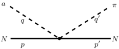
(a)

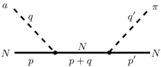
(b)

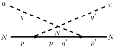
(c)

Figure 1: Tree level contributions to $aN\to\pi N$ without the $\Delta$ intermediate state.

The contact interaction, Fig. 1a, only gives a contribution to $B^{-}$ and is free of any kinematic variable:

$$B^{-}_{\text{\ref{fig:contact}}}=\frac{c_{u-d}}{2f_{a}F_{\pi}}\,.$$ (41)

This means that the contact interaction is solely present in the $ap\to\pi^{+}n$ and $an\to\pi^{-}p$ processes, but absent in any process involving the neutral pion. For the diagrams of Figures 1b and 1c, one gets

$$\begin{split}A^{+}_{\text{\ref{fig:ns},\ref{fig:ncrossed}}}&=\frac{g_{A}^{2}c_{u-d}m_{N}}{f_{a}F_{\pi}},\\ B^{+}_{\text{\ref{fig:ns},\ref{fig:ncrossed}}}(s,t)&=-\frac{g_{A}^{2}c_{u-d}m_{N}^{2}}{f_{a}F_{\pi}}\left(\frac{1}{s-m_{N}^{2}}-\frac{1}{u-m_{N}^{2}}\right),\\ A^{3+}_{\text{\ref{fig:ns},\ref{fig:ncrossed}}}&=\frac{g_{A}g_{0}^{i}c_{i}m_{N}}{f_{a}F_{\pi}},\\ B^{3+}_{\text{\ref{fig:ns},\ref{fig:ncrossed}}}(s,t)&=-\frac{g_{A}g_{0}^{i}c_{i}m_{N}^{2}}{f_{a}F_{\pi}}\left(\frac{1}{s-m_{N}^{2}}-\frac{1}{u-m_{N}^{2}}\right),\\ A^{-}_{\text{\ref{fig:ns},\ref{fig:ncrossed}}}&=0,\\ B^{-}_{\text{\ref{fig:ns},\ref{fig:ncrossed}}}(s,t)&=-\frac{g_{A}^{2}c_{u-d}m_{N}}{2f_{a}F_{\pi}}\left[1+2m_{N}\left(\frac{1}{s-m_{N}^{2}}+\frac{1}{u-m_{N}^{2}}\right)\right],\end{split}$$ (42)

where $u$ needs to be understood as $u(s,t)$ via Eq. (5). In the appendix, we give a different expression of these contributions in terms of the axion-nucleon coupling constants $g_{an}$ and $g_{ap}$ for each of the four possible $aN\to\pi N$ channels. However, for the study of the $P_{33}$ partial wave, it is not expedient to rewrite them in terms of $g_{an}$ and $g_{ap}$, because after forming the difference Eq. (14), one can nicely see that the isoscalar terms $\propto c_{i}$ stemming from $a_{\mu,i}^{(s)}$ drop out, leaving only the isospin violating portion $\propto c_{u-d}$ that originates from $a_{\mu}$. This fact makes it easy to show (as will be done below) that in the case of the $P_{33}$ partial wave the KSVZ axion can be treated as a special case of the DSFZ axion.

III.2 Intermediate Delta resonance

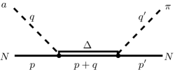
(a)

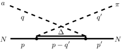
(b)

Figure 2: Tree-level contributions to $aN\to\pi N$ with an intermediate $\Delta$ state.

Including the $\Delta$ leads to the diagrams shown in Fig. 2. As the two diagrams are related by crossing, it is convenient to define

$$\begin{split}A_{\Delta}(s,t)=\frac{2g^{2}c_{u-d}}{3f_{a}F_{\pi}}\Biggl{\{}&\frac{2z_{0}}{3m_{\Delta}^{2}}\left[m_{\Delta}+\left(m_{N}+2m_{\Delta}\right)z_{0}\right]\left(s-m_{N}^{2}\right)+\frac{1}{s-\mu_{\Delta}^{2}}\biggl{[}\left(m_{N}+m_{\Delta}\right)\left(\frac{1}{2}\left[m_{a}^{2}+M_{\pi}^{2}-t\right]-\frac{1}{3}\left[s-m_{N}^{2}\right]\right)\\ &-\frac{1}{6m_{\Delta}^{2}}\biggl{(}\left(m_{N}+m_{\Delta}\right)\left(\left[m_{a}^{2}+M_{\pi}^{2}\right]\left[s-m_{N}^{2}\right]+m_{a}^{2}M_{\pi}^{2}\right)+m_{a}^{2}M_{\pi}^{2}m_{\Delta}+m_{N}\left(s-m_{N}^{2}\right)^{2}\biggr{)}\biggr{]}\Biggr{\}},\end{split}$$ (43)

and

$$\begin{split}B_{\Delta}(s,t)=\frac{2g^{2}c_{u-d}}{3f_{a}F_{\pi}}\Biggl{\{}&-\frac{z_{0}}{3m_{\Delta}^{2}}\biggl{[}m_{a}^{2}+M_{\pi}^{2}+2\left(s-m_{N}^{2}\right)\left(1+z_{0}\right)+4m_{N}m_{\Delta}\left(1+z_{0}\right)+4m_{N}\left(m_{N}+m_{\Delta}\right)z_{0}\biggr{]}\\ &+\frac{1}{s-\mu_{\Delta}^{2}}\biggl{[}\frac{1}{2}\left[m_{a}^{2}+M_{\pi}^{2}-t\right]-\frac{1}{6}m_{a}^{2}+\frac{1}{6m_{\Delta}}\left(m_{N}+m_{\Delta}\right)\left(4m_{N}m_{\Delta}-M_{\pi}^{2}\right)\\ &-\frac{1}{6m_{\Delta}^{2}}\Bigl{[}\left(m_{a}^{2}+M_{\pi}^{2}+2m_{N}m_{\Delta}\right)\left(s-m_{N}^{2}\right)+m_{a}^{2}\left(m_{N}m_{\Delta}+M_{\pi}^{2}\right)+\left(s-m_{N}^{2}\right)^{2}\Bigr{]}\biggr{]}\Biggr{\}}.\end{split}$$ (44)

Here the axion mass terms are kept explicitly though they, being tiny for the standard QCD axion models, can be safely neglected.

Then one can combine both diagrams and obtains the following expressions

$$\begin{split}A_{\Delta}^{+}(s,t)&=A_{\Delta}(s,t)+A_{\Delta}(u,t),\\ B_{\Delta}^{+}(s,t)&=B_{\Delta}(s,t)-B_{\Delta}(u,t),\\ A_{\Delta}^{-}(s,t)&=-\frac{1}{2}\left[A_{\Delta}(s,t)-A_{\Delta}(u,t)\right],\\ B_{\Delta}^{-}(s,t)&=-\frac{1}{2}\left[B_{\Delta}(s,t)+B_{\Delta}(u,t)\right]\,,\end{split}$$ (45)

where again $u=u(s,t)$. Note that there is no contribution to $T^{3+}$. Equations (43) and (44) have a pole appearing at c.m. energies around the $\Delta$ mass squared. In order to circumvent any unnecessary subtleties related to this, we use a Breit-Wigner propagator with a complex mass squared

$$\mu_{\Delta}^{2}=m_{\Delta}^{2}-im_{\Delta}\Gamma_{\Delta}$$ (46)

with $m_{\Delta}\approx 1232$ MeV and $\Gamma_{\Delta}\approx 117\,\text{MeV}$ the Breit-Wigner mass and width of the $\Delta$ resonance. A more refined treatment could e.g. be given by including the $\Delta$ self-energy in the complex mass scheme, but that is not required here.

III.3 Pion rescattering

Another sort of diagram that contributes is shown in Fig. 3. As in the previous diagrams, the left (smaller) vertex leads to an axion-pion conversion (so this vertex basically comprises the contributions of Fig. 1). This pion consequently gets rescattered in the ordinary $\pi N$ scattering. The latter (larger) vertex treated in a proper way also includes contributions from the $\Delta$ baryon. As this is an often studied process, we can base the treatment of this diagram on previous results. In particular, we will adopt the method and results of Refs. [42, 43].

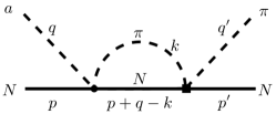
Figure 3: The pion rescattering diagram for $aN\to\pi N$.

The diagrams that contribute to the $\pi N$ scattering at this order are basically the same as the ones discussed in the previous subsections, but with the axion replaced by another pion. Using Eq. (11) and Eq. (17) leads to a projection to the $P_{33}$ partial wave. We do not repeat the results for the diagrams here, they can be found in Ref. [42], Eqs. (3.4) and (3.9). Moreover, we also adopt the results for the renormalized chiral pion loops obtained in heavy baryon CHPT (HBCHPT) from [44] (which are needed for the unitarization, see below).

As the $\pi N$ scattering above threshold and below the appearance of inelastic reactions fulfills the unitarity relation (here $W=\sqrt{s}$, the c.m. energy)

$$\operatorname{Im}T_{l\pm}^{I}(W)=\frac{|\mathbf{q}|}{8\pi W}|T_{l\pm}^{I}(W)|^{2},$$ (47)

the pole in the $\Delta$ propagator can be treated in a more systematic way than the one we used in Sec. III.2 for the $aN\to\pi N$ reaction. In particular, a suitable unitarization technique can be used to restore unitarity which is otherwise only fulfilled perturbatively in CHPT. The method used in Ref. [42] is the $N/D$ method [45, 46]. In a nutshell, it is based on the observation that the unitarity relation leads to a right-hand cut in the partial wave $T$-matrix such that one can write down a dispersion relation for the inverse amplitude with some extra terms which are free of any right-hand cuts. These can be matched to the amplitudes obtained from CHPT. This effectively corresponds to a resummation of the relevant diagrams. Possible double counting can be avoided by the matching procedure discussed in Ref. [43]. The integral of the dispersion relation can be performed analytically and is basically given by the known two-point loop function involving one pion and one nucleon,

$$g(s)= \,\frac{1}{16\pi^{2}}\left\{a_{0}(\mu)+\left(1-\frac{w}{m_{N}}\right)\log\left(\frac{M_{\pi}^{2}}{\mu^{2}}\right)\right.$$

$$\left.-x_{+}\log\left(\frac{x_{+}-1}{x_{+}}\right)-x_{-}\log\left(\frac{x_{-}-1}{x_{-}}\right)\right\},$$ (48)

at a renormalization scale $\mu$. We take $\mu$ as the nucleon mass, and any change in $\mu$ can be reabsorbed by the subtraction constant $a_{0}(\mu)$. Furthermore, $w$ is the c.m. pion energy and

$$x_{\pm}=\frac{s+m_{N}^{2}-M_{\pi}^{2}}{2s}\pm\frac{1}{2s}\sqrt{\lambda(s,m_{N}^{2},M_{\pi}^{2})}\,.$$ (49)

The matching procedure for unitarizing the leading one-loop $\mathcal{O}(p^{3})$ amplitude with the $\Delta$ resonance leads to

$$T^{I,l\pm}_{\pi N}=\frac{1}{\left(T^{I,l\pm}_{\text{tree}}+T^{I,l\pm}_{\text{loop}}+T^{I,l\pm}_{\Delta}+\frac{2\sqrt{s}}{E_{\mathbf{p}}+m_{N}}\left(T^{I,l\pm}_{\text{LO}}\right)^{2}g(s)\right)^{-1}+g(s)},$$ (50)

which indeed fulfills Eq. (47). Note that the tree contributions $T^{I,l\pm}_{\text{tree}}$ and $T^{I,l\pm}_{\Delta}$ for the resonance are taken as being the full relativistic ones, whereas $T^{I,l\pm}_{\text{LO}}$ is only the very leading order HBCHPT amplitude.

Returning to pion axioproduction, we performed a full reanalysis of the phase shift $\delta_{l\pm}^{I}$ defined by

$$T_{l\pm}^{I}(W)=\frac{8\pi W}{|\mathbf{q}|}\exp(i\delta_{l\pm}^{I})\sin(\delta_{l\pm}^{I})$$ (51)

in order to use these results for the rescattering diagram and in order to determine accurate values for the coupling constants $g$ and $z_{0}$ of Eq. (38) and $a_{0}$ of Eq. (III.3). The latter goal is achieved by fitting the resulting $P_{33}$ phase shift to the results of the Roy–Steiner analysis of the $\pi N$ scattering [47]. As input values we used the isospin-averaged nucleon mass $m_{N}=(m_{n}+m_{p})/2=938.92\,\text{MeV}$, the isospin-averaged pion mass $M_{\pi}=138.03\,\text{MeV}$, $F_{\pi}=92.4\,\text{MeV}$, and $m_{\Delta}=1232\,\text{MeV}$. The value of $g_{A}$ is discussed below when it comes to the determination of the axion-baryon couplings in Sec. IV. The fit to the phase shift values of $W\lesssim 1.3\,\text{GeV}$ yields

$$g=1.249(16),\quad z_{0}=-0.21(56),\quad a_{0}=-0.959(12)$$ (52)

and is shown in Fig. 4.

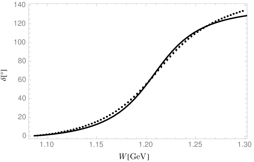
Figure 4: The $\pi N$ phase shift $\delta$ in the $P_{33}$ channel (solid line) fitted to the results of the Roy–Steiner analysis (dots) from [47].

Finally, the rescattering diagram is evaluated by

$$\begin{split}T^{33}_{\rm rescatt.}(s)=&\Bigl{(}T^{33,\text{tree}}_{ap\to\pi^{0}p}(s)g(s,M_{\pi^{0}})\\ &\quad-\frac{1}{\sqrt{2}}T^{33,\text{tree}}_{ap\to\pi^{+}n}(s)g(s,M_{\pi^{+}})\Bigr{)}T^{33}_{\pi N}(s)\,,\end{split}$$ (53)

where $g(s,M_{\pi^{+,0}})$ is the pion-nucleon loop function Eq. (III.3) with the meson (nucleon) mass being the charged and neutral pion (neutron and proton) mass, respectively. $T^{33,\text{tree}}_{aN\to\pi N}$ denotes the partial wave projected amplitudes of Sec. III.1 and $T^{33}_{\pi N}$ the unitarized $P_{33}$ partial wave amplitude just discussed. We consider the usage of the latter appropriate even though it is derived using on-shell kinematics, as the off-shell effects are certainly subleading [48].

The expression in the parentheses is the proper way of getting the isospin violating part of the amplitude, as discussed in Sec. II.2, see Eq. (15), i.e. by taking the difference of the amplitudes and the difference in the charged and neutral pion/nucleon masses. If one neglects this mass difference, one might as well use Eq. (14) instead yielding

$$T^{33}_{\rm rescatt.}(s)=T^{33,\text{tree}}_{aN\to\pi N}(s)g(s,M_{\pi})T^{33}_{\pi N}(s),$$ (54)

where $T^{33,\text{tree}}_{aN\to\pi N}$ now is the $j=\tfrac{3}{2}$ projection of $T^{I=3/2}$, Eq. (14), and $M_{\pi}$ is the isospin averaged pion mass. In fact, this latter approximation gives an average deviation of only $\lesssim 2\%$ in comparison to Eq. (53), which is valid for the KSVZ axion and the DFSZ axion at $\sin^{2}\beta\lesssim 0.95$. Only for values $\sin^{2}\beta\to 1$ the deviation becomes more pronounced at c.m. energies $W\gtrsim 1.15\,\text{GeV}$ reaching a maximum of about $15\%$. This means that Eq. (54) is a very good approximation for the vast majority of cases.

IV Results

Let us take the last result of the previous section as a starting point for the discussion of the overall results of this study. If one indeed takes the approximation of equal pion/nucleon masses, then Eq. (12) causes that any dependence on the isoscalar couplings $g_{0}^{i}c_{i}$ is canceled and any dependence on the axion-nucleon coupling $g_{aN}$ in this process reduces to a dependence on $g_{A}c_{u-d}$ only, which reflects that this part of the coupling enforces the isospin violation needed to enable the $\Delta$ resonance appearance. For the same reason, the diagrams of Fig. 2 with the explicit $\Delta$ solely depend on $c_{u-d}$ and not on the $c_{i}$’s. This has two consequences: First, the total amplitude for the DFSZ axion with $\sin^{2}\beta$ in the interval $[0,1]$ and that for the KSVZ model will be $\propto c_{u-d}$; they have entirely the same shape, and only the magnitude changes as $\sin^{2}\beta$ is varied. Second, as $c_{u-d}$ only depends on the difference $X_{u}-X_{d}$, one can easily determine a value for $\sin^{2}\beta$ such that $c_{u-d}^{\text{DFSZ}}(\sin^{2}\beta)=c_{u-d}^{\text{KSVZ}}$, which is accomplished when $\sin^{2}\beta=\tfrac{1}{2}$ (see Eq. (26)). The $aN\to\pi N$ scattering amplitude in the $P_{33}$ channel for the KSVZ axion is hence exactly the same as that for the DFSZ axion at $\sin^{2}\beta=\tfrac{1}{2}$. As the deviation from this approximation is only $\lesssim 2\%$, this remains basically true even if one considers Eq. (53) instead of Eq. (54).

For the calculation of the final scattering amplitude, we make use of the nucleon matrix elements in order to determine the isovector and isoscalar axial-vector couplings

$$g_{A} = \Delta u-\Delta d\,,$$

$$g_{0}^{u+d} = \Delta u+\Delta d\,,$$ (55)

$$g_{0}^{q} = \Delta q\,,\text{ for }q=s,c,b,t\ ,$$

where $s^{\mu}\Delta q=\langle p|\bar{q}\gamma^{\mu}\gamma_{5}q|p\rangle$, with $s^{\mu}$ the spin of the proton. Of course, for the approximation discussed in the previous paragraph, only the value of $g_{A}$ is of interest. For these matrix elements and $z$ and $w$ appearing in Eq. (26), we take the recent values from Ref. [49],

$$\begin{array}[]{rlrlrl}\Delta u&=0.847(50),\\ \Delta d&=-0.407(34),\\ \Delta s&=-0.035(13),\\ z&=0.485(19),\\ w&=0.025(1),\\ \end{array}$$ (56)

and ignore $\Delta q$ for $q=c,b,t$.

In Fig. 5, we show the partial wave cross sections $\sigma^{33}_{aN\to\pi N}$ consisting of all the contributions discussed in Sec. III, for both with the approximation Eq. (54) and without it. Actually, the cross sections are multiplied by the factor $f_{a}^{2}$ in order to get rid of the unknown prefactor $1/f_{a}^{2}$. This unknown quantity also appears implicitly in the terms containing the axion mass in Eq. (43) and (44), but has practically no effect as the axion mass $\propto 1/f_{a}$ can safely be neglected for the typical QCD axion window, Eq. (1). However, this prefactor has to be kept in mind when considering the strength of the amplitudes in Fig. 5.

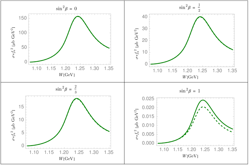
Figure 5: The $aN\to\pi N$ partial wave cross section of the $P_{33}$ channel versus the c.m. energy $W$ for the DFSZ axion at different values of $\sin^{2}\beta$ and the KSVZ axion (which corresponds to $\sin^{2}\beta=\frac{1}{2}$, see main text). The dashed curve corresponds to the approximated case based on Eq. (54).

As anticipated, the curves for different values of $\sin^{2}\beta$ are identical up to the order of magnitude. As the absolute value of $c_{u-d}$ is a linearly decreasing function of $\sin^{2}\beta$, the magnitude steadily decreases, which makes a DFSZ axion with $\sin^{2}\beta\to 1$ the most unfavorable candidate for detection. As expected from the description at the end of the previous section, there is almost no visual deviation of the curves with approximation Eq. (54) and without it. Only for $\sin^{2}\beta=1$ this deviation becomes recognizable but is still a minor effect. Note that the figures for the limit values of $\sin^{2}\beta=\{0,1\}$ are given rather for illustrative purposes, as in realistic DFSZ models perturbative constraints from the heavy quark Yukawa couplings yield an allowed range $[0.25,170]$ for $\cot\beta$ [21] corresponding to approximately $\sin^{2}\beta\in[0.00,0.94]$.

As a result, there is indeed a considerable enhancement of the $P_{33}$ partial wave cross section in the region of the $\Delta$ resonance, but this enhancement is considerably weaker than previously assumed by Carenza et al. [16], who estimated the cross section via $f_{a}^{2}\sigma_{aN\to\pi N}\approx F_{\pi}^{2}\sigma_{\pi N\to\pi N}$ taking a value of $100\,\mathrm{mb}$ for $\sigma_{\pi N\to\pi N}$. This estimation suggests a peak value $f_{a}^{2}\sigma_{aN\to\pi N}\approx 1\,\mathrm{mb}\,\mathrm{GeV}^{2}$. The discrepancy between the results of Fig. 5 and such estimation can be explained by the fact that ${aN\to\pi N}$ in the $\Delta$ sector is primarily an isospin breaking process, which always comes with an extra suppression. It is worthwhile to notice that the suppression of the isospin breaking here, characterized by the factor $(1-z)/(1+z)=(m_{d}-m_{u})/(m_{d}+m_{u})\approx 0.34$ for the model-independent part of $c_{u-d}$ (see Eq. (27)), is much milder than that for usual isospin breaking in hadronic processes, characterized by $(m_{d}-m_{u})/m_{s}$ or $(m_{d}-m_{u})/\Lambda_{\text{QCD}}$. Thus, the results given in Ref. [16] are to be multiplied by a factor $10^{-1}$ to $10^{-5}$, depending on the value of the model-dependent factor $\sin^{2}\beta$, that is a suppression by at least one order of magnitude. Then the number of pions produced via $aN\to\pi N$ through the $\Delta$ resonance in a megaton water Cherenkov detector will be at most $\mathcal{O}(100)$ using the axion luminosity estimated in Ref. [16] for axions emitted from a supernova at 1 kiloparsec.

V Summary

In this study we presented an analysis of the pion axioproduction $aN\to\pi N$ with an intermediate $\Delta$ resonance. We included the $\Delta$ resonance in two different ways: First, we used the chiral interaction Lagrangian for the $\Delta$ to bring the axion explicitly into contact with the resonance, and, second, we used the well-known results of $\pi N$ elastic scattering with $\Delta$ to include it implicitly in the form of the rescattering diagram in Fig. 3.

As the $\Delta$ is a spin-$\tfrac{3}{2}$ and isospin-$\tfrac{3}{2}$ particle, it shows its full leverage effect in the $P_{33}$ partial wave, which is why we concentrated on a study of this particular partial wave. For the same reason, this interaction is essentially an isospin violating process, as the axion is an isosinglet. We have shown that an approximation that concentrates on this isospin violation and that neglects any isoscalar coupling, while at the same time ignoring the pion and nucleon isospin mass splittings, is still very accurate unless $\sin^{2}\beta$ approaches $1$ in the DFSZ axion model (where it still gives quite good results). In this way, it is shown that the partial wave amplitude for the KSVZ axion equals that for the DFSZ axion at $\sin^{2}\beta=\tfrac{1}{2}$.

Finally, the enhancement of the amplitude anticipated by Carenza et al. [16] is indeed present in the region of the $\Delta$ resonance, although it is considerably weaker than their naive estimation by at least an order of magnitude. This is basically a consequence of the isospin breaking suppression which though is much milder than that for usual isospin breaking hadronic processes. Therefore, it might be interesting to check whether other isospin-1/2 resonances such as the $N^{*}(1440)$ Roper resonance would provide an additional enhancement of the $aN\to\pi N$ cross section, as it is accessible without isospin breaking. The next step would hence be to investigate the impact of such resonances on the $aN\to\pi N$ reaction and consequently on the axion production in stellar objects, and whether this might be exploited to give fresh perspectives on experimental axion searches.

*

Appendix A Amplitudes of the leading order tree graphs

In this appendix, we give the full expression of the leading order tree graph amplitudes of the four $aN\to\pi N$ channels. Using the abbreviation

$$R_{\mu}=\frac{1}{2}\left(q_{\mu}+q_{\mu}^{\prime}\right),$$ (57)

the contact contribution reads

$$T^{\text{\ref{fig:contact}}}_{aN\to\pi^{0}N} =\phantom{-}0,$$ (58)

$$T^{\text{\ref{fig:contact}}}_{ap\to\pi^{+}n} =\phantom{-}\frac{c_{u-d}}{\sqrt{2}f_{a}F_{\pi}}\bar{u}(p^{\prime})\,\not{R}\,u(p),$$ (59)

$$T^{\text{\ref{fig:contact}}}_{an\to\pi^{-}p} =-\frac{c_{u-d}}{\sqrt{2}f_{a}F_{\pi}}\bar{u}(p^{\prime})\,\not{R}\,u(p),$$ (60)

where the superscript refers to Fig. 1. For the other two diagrams Fig. 1b and  1c one gets

$$T^{\text{\ref{fig:ns},\ref{fig:ncrossed}}}_{ap\to\pi^{0}p} =\phantom{-}\frac{g_{A}m_{N}g_{ap}}{f_{a}F_{\pi}}\bar{u}(p^{\prime})\Biggl{\{}1-m_{N}\left(\frac{1}{s-m_{N}^{2}}-\frac{1}{u-m_{N}^{2}}\right)\not{R}\Biggr{\}}u(p),$$ (61)

$$T^{\text{\ref{fig:ns},\ref{fig:ncrossed}}}_{an\to\pi^{0}n} =-\frac{g_{A}m_{N}g_{an}}{f_{a}F_{\pi}}\bar{u}(p^{\prime})\Biggl{\{}1-m_{N}\left(\frac{1}{s-m_{N}^{2}}-\frac{1}{u-m_{N}^{2}}\right)\not{R}\Biggr{\}}u(p),$$ (62)

$$T^{\text{\ref{fig:ns},\ref{fig:ncrossed}}}_{ap\to\pi^{+}n} =\frac{g_{A}}{\sqrt{2}f_{a}F_{\pi}}\bar{u}(p^{\prime})\Biggl{\{}2m_{N}g_{0}^{i}c_{i}-\left[g_{A}c_{u-d}+2m_{N}^{2}\left(\frac{g_{ap}}{s-m_{N}^{2}}-\frac{g_{an}}{u-m_{N}^{2}}\right)\right]\not{R}\Biggr{\}}u(p),$$ (63)

$$T^{\text{\ref{fig:ns},\ref{fig:ncrossed}}}_{an\to\pi^{-}p} =\frac{g_{A}}{\sqrt{2}f_{a}F_{\pi}}\bar{u}(p^{\prime})\Biggl{\{}2m_{N}g_{0}^{i}c_{i}+\left[g_{A}c_{u-d}-2m_{N}^{2}\left(\frac{g_{an}}{s-m_{N}^{2}}-\frac{g_{ap}}{u-m_{N}^{2}}\right)\right]\not{R}\Biggr{\}}u(p).$$ (64)

Here, $g_{an}$ and $g_{ap}$ are the usual axion-nucleon couplings given in Eq. (33).