Semi-supervised 3D Object Detection via Temporal Graph Neural Networks

Abstract

3D object detection plays an important role in autonomous driving and other robotics applications. However, these detectors usually require training on large amounts of annotated data that is expensive and time-consuming to collect. Instead, we propose leveraging large amounts of unlabeled point cloud videos by semi-supervised learning of 3D object detectors via temporal graph neural networks. Our insight is that temporal smoothing can create more accurate detection results on unlabeled data, and these smoothed detections can then be used to retrain the detector. We learn to perform this temporal reasoning with a graph neural network, where edges represent the relationship between candidate detections in different time frames. After semi-supervised learning, our method achieves state-of-the-art detection performance on the challenging nuScenes [3] and H3D [19] benchmarks, compared to baselines trained on the same amount of labeled data. Project and code are released at https://www.jianrenw.com/SOD-TGNN/.

1 Introduction

3D object detection is an essential and fundamental problem in many robotics applications, such as autonomous driving [31], object manipulation [29], and augmented reality [32]. In recent years, many deep learning-based approaches for point cloud-based 3D object detection [34, 13, 42] have emerged and achieved high performances on various benchmark datasets [25, 3, 4, 19]. Despite the impressive performances, most of the existing deep learning-based approaches for 3D object detection on point clouds are strongly supervised and require the availability of a large amount of well-annotated 3D data that is often time-consuming and expensive to collect.

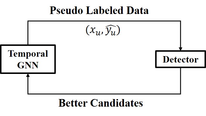
Figure 1: Semi-supervised 3D Object Detection via Temporal Graph Neural Networks. Our method utilizes the rich spatiotemporal information from point cloud videos to perform semi-supervised learning to train a single frame object detector. This detector can be used to generate better candidates, which will in turn lead to better psuedo labels.

Semi-supervised learning [26] is a promising alternative to supervised learning for point cloud-based 3D object detection. This is because semi-supervised learning requires only a limited amount of labeled data, instead relying on large amounts of unlabeled data to improve performance. The challenge with semi-supervised learning is to determine how to make use of the unlabeled data to improve the performance of the detector.

In most applications, point clouds are recorded over time as a data stream. A point cloud video contains richer spatiotemporal information than a single frame. Our insight is that this spatiotemporal information can be exploited to correct inaccurate predictions. For example, a false negative (missing) detection can be identified if the same object is detected in adjacent frames but is missing in the current frame. A false positive detection can be identified if the detection is isolated i.e. a corresponding detection occurs neither in the previous nor the subsequent frame. A misalignment can be identified if the alignment differs significantly between successive video frames (see Figure 2 for examples).

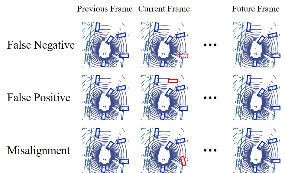
Figure 2: Detections in Point Cloud Videos. 3D object detectors usually suffer from false negatives, false positives and misalignment due to the sparse nature of LiDAR data. However, these failures can always be detected by exploiting the rich spatiotemporal information in point cloud videos. For example, a false negative (red box in the top row) can be identified if the same object is detected in adjacent frames but is only missing in the current frame. A false positive (red box in the middle row) can be identified if the detection isisolated i.e. a corresponding detection occurs neither in the previous nor the subsequent frame. A misalignment (red box in the bottom row) can be identified if the same object is detected in adjacent frames but the alignment differs significantly in the current frame. (Blue boxes show true positives, where the same object is detected in all adjacent frames).

In this paper, we propose utilizing the rich spatiotemporal information from point cloud videos to perform semi-supervised learning to train a single frame object detector (Figure 1). Specifically, we first build video graphs using a large amount of unlabeled point cloud videos, where each node represents a candidate detection predicted by a pretrained detector and each edge represents the relationship between the connected nodes in different time frames. A graph neural network is then used to refine these candidate detections using spatiotemporal information. These refined detections are treated as pseudo labels and are used to re-train a detector. This retrained detector can be used to generate better detections, which can again be refined in an iterative process of continual improvement.

A potential limitation with learning using pseudo labels generated from temporally smoothed detections is that these labels are not necessarily accurate. The detector may produce mistakes, and learning on these mistakes may lead to inferior 3D detections. We propose to explicitly tackle this problem by incorporating uncertainty into semi-supervised learning. Specifically, we propose to use the entropy of estimated detections as uncertainty weights for the semi-supervised loss. We demonstrate the efficacy of our method across a variety of large-scale benchmark datasets, including nuScenes [3] and H3D [19] and show state-of-the-art detection performance, compared to baselines trained on the same amount of labeled data.

The contributions of this paper are as follows:

1. We propose a novel framework for semi-supervised 3D object detection by leveraging the rich spatiotemporal information in 3D point cloud videos.

2. We propose a 3DVideoGraph for spatiotemporal reasoning in 3D point cloud videos.

3. We show that we can use the 3DVideoGraph with uncertainty loss weighting for semi-supervised training of 3D object detectors.

4. We demonstrate our method over two large-scale benchmark datasets and show state-of-the-art detection performance, compared to baselines trained on the same amount of labeled data.

2 Related Work

3D Object Detection

3D object detectors aim to predict 3D oriented bounding boxes around each object. A common approach to 3D object detection is to exploit the ideas that have been successful for 2D object detection [6, 5, 22, 7], which first find category-agnostic bounding box candidates, then classify and refine them. Existing works can be roughly categorized into three groups, which are birds-eye-view based methods [35, 14], voxel-based methods [41, 34], and point-based methods [13, 27]. Unlike these methods, our work focus on semi-supervised learning to improve a detector’s performance.

3D Video Object Detection

A few recent papers have incorporated spatiotemporal reasoning in 3D video object detection. 3DVID [37] proposes an Attentive Spatiotemporal Transformer GRU (AST-GRU) to aggregate spatiotemporal information across time. Similarly, 3DLSTM [9] proposes a sparse LSTM to aggregate features across time. These works show great potential by utilizing the rich spatiotemporal information in point cloud videos. However, they use memory-intensive sequence models to utilize the temporal information; as a result, only three consecutive frames can be input to the model due to memory limitations [37], which makes it hard to reason about complex spatiotemporal information. In contrast, our graph neural network representation can reason over much longer sequences. Further, we show how such spatiotemporal reasoning can be combined with uncertainty estimates for semi-supervised learning of a single-frame detector.

Semi-supervised Learning

Many approaches have been proposed for semi-supervised learning (SSL), which learns from a small labeled dataset combined with a much larger unlabeled dataset. One approach uses pseudo labels, also known as self-training. Self-training has been successfully applied to improve the state-of-the-art of many tasks, such as image classification [33], object detection [15], semantic segmentation [24]. These methods often involve a teacher which provides pseudo-labels for a student which learns from these pseudo-labels [1, 21]. However, these methods highly depend on the performance of teacher. which often makes incorrect predictions.

Another promising direction for SSL is self-ensembling, which encourages consensus among ensemble predictions of unknown samples under small perturbations of inputs or network parameters [40, 17, 28]. The student learns to perform better than the teacher due to its robustness to corruption. However, the improvement is limited since the teacher and student can use the same data to make predictions. In contrast, we propose to use spatiotemporal information to construct a better teacher, which is then used to train a student which has access to only single-frame information.

Spatiotemporal Reasoning

Most efforts in spatio-temporal reasoning focus on 2D semantic segmentation [36, 18, 20]. For example, Bao et al. [2] embed mask propagation into the inference of a spatiotemporal MRF model to improve temporal coherency. EGMN [16] employs an episodic memory network to store frames as nodes and capture cross-frame correlations by edges. However, these methods are computationally expensive even in 2D videos, which makes them infeasible to be adapted to 3D videos. In contrast, our temporal GNN is very computational efficient and memory efficient and thus can be applied to long sequences.

3 Approach

In this section, we elaborate on our method for semi-supervised 3D object detection. Our method consists of a teacher which performs spatiotemporal reasoning for 3D object detection; this teacher is then used to provide pseudo labels to train a student which takes as input only a single frame (see Figure 3). We use uncertainty-aware training to handle incorrect pseudo labels produced by the teacher.

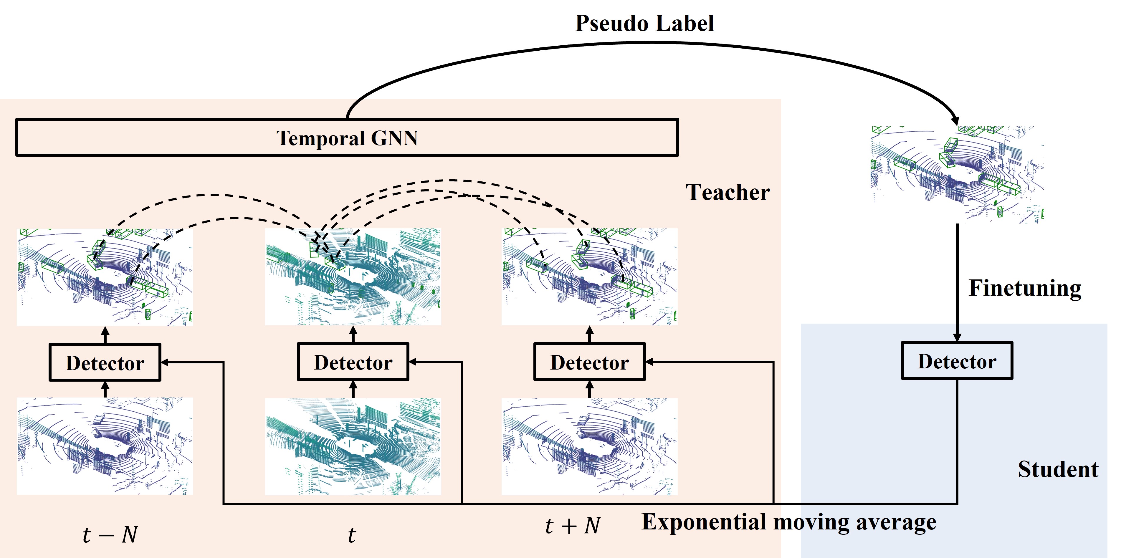
Figure 3: Overview of Semi-supervised 3D Object Detection via Temporal Graph Neural Networks: The teacher consists of a 3D object detector and a graph neural network for spatiotemporal reasoning. The 3D object detector takes a single point cloud frame as input and outputs candidate detections. The graph neural network takes candidate detections from a sequence of point clouds as input and outputs refined detection scores. These pseudo labeled point clouds are then combined with labeled point clouds to train the student. The 3D object detection module of the teacher and the student are with the same architecture. And the parameters of the 3D object detection module of the teacher are the exponential moving average of the continually updated student network parameters. This updated detector is used to generate better detections, which is further used to refine the spatiotemporal reasoning module. The iterative refinement of student and teacher can lead to a continual improvement.

3.1 Teacher Network: GNN for Spatiotemporal Reasoning

We first describe our teacher network, which uses spatiotemporal reasoning to provide pseudo labels on unlabeled data. These pseudo labels are then used to train a student which takes as input single-frame data.

Our teacher network consists of two modules: a 3D object detection module, and a spatiotemporal reasoning module. The 3D object detection module can be any existing 3D object detector, which is initially trained from only a limited amount of labeled data. We then input each frame to the 3D object detector to find detected objects in the scene. We filter the output of this detector with a fairly low threshold (we use a confidence of 0.1 in our experiments) to create a large set of candidate detections in the scene. However, these predictions are always noisy and inaccurate.

To smooth these detections and create more accurate pseudo labels, we propose a novel spatiotemporal reasoning module: we build a video graph over the frames of the 3D video (sequence of point clouds), and use a Graph Neural Network (GNN) to output new scores for each detection node based on the principle of spatiotemporal consistency. This spatiotemporal reasoning module is trained on the same labeled data as the 3D object detection module.

Specifically, we extract a set of high-level features of each candidate detection as node features ($x$) for the 3D video graph. These high level features include (1) the detection score, (2) the number of points in the detection box, and (3) the size of the detection box (width, length, and height). In total, our node features are 5-dimensional.

After feature extraction, we have a node feature vector for each candidate detection in each frame of a video. To connect nodes across frames, we use the detection’s estimated velocity, which is often predicted by the 3D object detector [42, 31, 38]. We project the node to its neighboring frames based on its estimated velocity, as follows:

$$\hat{p}^{i}_{t+N}=v^{i}_{t}\cdot(T_{t}-T_{t+N})+p^{i}_{t},$$ (1)

where $\hat{p}^{i}_{t+N}$ represents the predicted position of object $i$ in frame $t+N$, $p^{i}_{t}$ and $v^{i}_{t}$ represents the estimated position and velocity of object $i$ in frame $t$, and $T_{t}$ and $T_{t+N}$ represents the timestamp of frame $t$ and frame $t+N$. We then calculate the distance between the predicted position of object $i$ ($\hat{p}^{i}_{t+N}$) with all detections in frame $t+N$. All detections whose distance to the predicted position are smaller than a threshold are connected to node $i$. Each node is connected to all such neighboring nodes in the neighboring frames from $t-N$ and $t+N$. We also add the following edge features ($e$) to the 3D video graph: (1) the distance between the predicted center positions of each pair of detection boxes (1-dimensional), (2) the difference in the sizes along each dimension (3-dimensional), and (3) the difference in bounding box orientations (1-dimensional). In total, our edge features are 5-dimensional.

Finally, our GNN takes the node feature and edge feature as input, and it outputs a new detection score $s_{i}$ for the $i^{th}$ candidate detection. The graph neural network operations can be written as:

$$x^{k}_{i}=\gamma^{k}(x^{k-1}_{i},\cup_{j\in\mathcal{N}(i)}\phi^{k}(x^{k-1}_{i},x^{k-1}_{j},e_{j,i})),$$ (2)

where $\gamma^{k}$ denotes the $k^{th}$-step updating network, $\phi^{k}$ denotes the $k^{th}$-step message network ($k^{th}$-layer of the graph neural network), $\cup$ denotes the message aggregation function, $x^{k-1}_{i}$ and $x^{k-1}_{j}$ denotes node features of node $i$ and $j$ in layer $(k-1)$, and $e_{j,i}$ denotes the edge features of node $j$ and node $i$, which remains unchanged for all layers. The output of the final update is the new detection score $s_{i}$.

$$s_{i}=x_{i}^{K},$$ (3)

where $x_{i}^{K}$ represents the final update (output of the final layer) of node $i$.

The GNN is trained end-to-end using the Binary Cross Entropy Loss (BCE). The spatio-temporal reasoning of the GNN allows the network to output more accurate detections than those of the original 3D object detector.

These refined detections are treated as pseudo labels and are used to train a student (a 3D object detector). For simplicity, the 3D object detection module of the teacher and the student are with the same architecture. And the parameters of the 3D object detection module of the teacher $\theta^{T}$ are the exponential moving average (EMA) of the continually updated student network parameters $\theta^{S}$.

$$\theta_{t}^{T}=\alpha\theta_{t}^{S}+(1-\alpha)\theta_{t-1}^{T},$$ (4)

where the coefficient $\alpha$ represents the degree of weighting decrease, $\theta_{t}^{S}$ represents the student network parameters after iteration $t$.

This updated detector is used to generate better detections, which is further used to refine the spatiotemporal reasoning module. The iterative refinement of student and teacher can lead to a continual improvement. Please refer to Section 4.2 for more details on the training procedure.

3.2 Graph Augmentation

To prevent the graph neural network from overfitting, we use data augmentation. It’s worth noticing all these augmentations are only applied to the limited amount of labeled data since the spatiotemporal reasoning module is only trained on the labeled data. We propose three novel data augmentation techniques.

Copy-and-Paste

A copy-and-paste augmentation scheme is widely used in many popular single-frame object detectors including SECOND [34], PointPillars [13], and CenterPoint [38], which crops ground truth bounding boxes from other frames and pastes them onto the current frame’s ground plane. Unlike previous methods, we propose trajectory-level copy and paste. We first assign each object an identity based on the its center distance to the closest ground truth object Then, detections with same identity form a trajectory; a random clip of the trajectory is copied into a new video with a random starting frame. Similarly, we also randomly remove trajectories from current video as a form of data augmentation.

Random Trim

To further increase the diversity of our data, we propose to randomly select the first frame and the last frame from a video to form the sequence of frames used in the graph.

Random Noise

We also propose to add random noise to the location, size, orientation and detection scores of individual detections. This is to simulate errors of a pre-trained object detector on more diverse unlabelled data. The noise values for the location and size are uniformly sampled from $\pm 10\%$ of the bounding box size, while the orientation noise is uniformly sampled from $\pm 10^{\circ}$. The detection score noise is uniformly sampled from $\pm 0.15$ and is only applied to detections in the middle of a trajectory (not detections at the beginning or end of a trajectory).

3.3 Uncertainty-aware Semi-supervised Training

One of the most prominent challenges in training on pseudo labels is that they are not guaranteed to be accurate. Our solution is to leverage uncertainty in the pseudo labels. For examples with high uncertainty, we discount the contribution of the corresponding example during training. This is intended to reduce the effect of incorrect labels in semi-supervised training.

We propose a method for estimating the amount of uncertainty of each pseudo label during training time. To estimate uncertainty, we first obtain the new detection score $s_{i}$ from the temporal GNN mentioned in Section 3.1. However, these scores are not always well calibrated. In other words, the probability associated with the predicted label cannot reflect its ground truth correctness likelihood. To calibrate the prediction score, we adopt histogram binning [39], a simple non-parametric calibration method.

In short, all uncalibrated predictions $s_{i}$ are divided into mutually exclusive bins $B_{1}$,…, $B_{M}$. Each bin is assigned a calibrated score $\theta_{m}$; i.e. if $s_{i}$ is assigned to bin $B_{m}$, then the calibrated score $\hat{s_{i}}=\theta_{m}$. More precisely, for a suitably chosen M, we first define bin boundaries $0=a_{1}\leq a_{2}\leq...\leq a_{M+1}=1$, where the bin $B_{M}$ is defined by the interval $(a_{m},a_{m+1}]$. The prediction $\theta_{i}$ are chosen to minimize the bin-wise squared loss:

$$\mathop{min}\limits_{\{\theta_{i}\}}\sum_{m=1}^{M}\sum_{i=1}^{n}1(a_{m}\leq s_{i}\leq a_{m+1})(\theta_{m}-s_{i})^{2},$$ (5)

where $1$ is the indicator function. Given fixed bins boundaries, the solution to Eq. 5 results in $\theta_{m}$ that correspond to the average number of positive-class samples in bin $B_{m}$.

We then use the entropy [23] of the calibrated score $\hat{s_{i}}$ as a measure of uncertainty $u_{i}$:

$$u_{i}=-\hat{s}_{i}\log(\hat{s}_{i})-(1-\hat{s}_{i})\log(1-\hat{s}_{i})$$ (6)

This uncertainty is then used to weight the pseudo labels during training the student – any existing 3D object detector, which is always composed of a classification branch and a regression branch.

We first apply this uncertainty to the classification branch:

$$loss_{c}^{\prime}=\left\{\begin{array}[]{lr}-(1-u_{i})^{k}\log(p_{i}),&\textrm{if}\,\hat{s}_{i}>0.5\\ -(1-u_{i})^{k}\log(1-p_{i}),&\textrm{if}\,\hat{s}_{i}<0.5\\ \end{array}\right.$$ (7)

where $k$ is the focusing parameter $k\geq 0$ which helps the model focuses on the samples with low uncertainty and $p_{i}$ is the prediction of our student neural network.

We also apply the uncertainty to the bounding box regression branch:

$$loss_{r}^{\prime}=u_{i}\times\sum_{b\in(x,y,z,w,,l,h,\theta)}Dis(\Delta b)$$ (8)

where $\Delta b$ defines the regression residuals between psuedo-labels and student’s prediction, and $Dis$ defines the distance metric (e.g. Smooth L1 loss).

In total, the semi-supervised loss $loss_{s}$ is defined as a combination of uncertainty-weighted classification loss and regression loss:

$$loss_{s}=loss_{c}^{\prime}+loss_{r}^{\prime}$$ (9)

3.4 Gradual Semi-supervised Training and Iterative Refinement

To avoid the student learning from large amount of unreliable pseudo labels, we propose gradual semi-supervised training inspired by [12, 26, 8]. In a nutshell, the student is training with a mix of labelled and unlabelled data, while the amount of unlabelled data increase gradually in each iteration. After each iteration, we update the 3D object detection module of the teacher as a exponential moving average of the student. This updated detector is used to generate better detections. We then retrain the GNN on labeled data for better spatiotemporal reasoning. As the teacher keeps improving, the student can learn from a larger amount of more reliable pseudo labels each iteration. Thus, combining gradual semi-supervised training with iterative refinement of student and teacher can lead to a continual improvement.

4 Experiments

We evaluate our approach on 3D object detection on the nuScenes dataset [3] and Honda 3D dataset (H3D) [19] , which provide a series of sequence of 3D lidar pointcloud with annotated 3D bounding boxes. We also verify the effectiveness of each component of our method by performing an ablation analysis.

4.1 Dataset and Experiment Setup

To obtain enough unlabeled data for semi-supervised training, we re-split the nuScenes dataset as following. We use 50 scenes from nuScenes train for supervised training and 500 scenes from nuScenes train for semi-supervised training. For semi-supervised training, instead of using the ground truth labels, we use the pseudo labels generated by our proposed teacher network. We also use 150 scenes from nuScenes train as validation set. We pick the iteration with best performance on our validation set and reports its performance on 150 videos from nuScenes validation.

For H3D dataset, we use 50 scenes from H3D train for supervised training and 300 scenes from HRI Driving Dataset (HDD) for semi-supervised training, since H3D and HDD datasets have the same data distribution. We pick the iteration with best performance on 30 scenes from H3D validation and reports its performance on 80 videos from H3D test. We compare our methods with baselines using the official metric: mean Average Precision (mAP).

4.2 Training Details

Our teacher is composed of two modules: 3D object detection module and spatiotemporal reasoning module. We choose CenterPoint [38], a state-of-art 3D object detector as the detection module for both the teacher and the student. We use a 4-layer-GNN for the spatiotemporal reasoning and use the mean function for message aggregation (Eq 2). Node features and edge features are computed as described in Section 3.1. The distance threshold below which two detections in adjacent frames are connected is set to 10m. We use 4 preceding frames and 4 succeeding frames as adjacent frames (N = 4 as denoted in Section 3.1). Combined with the current frame, a node can be connected to 9 frames in total.

The student network is initialized from the 3D object detection module of the teacher trained on a small amount of labeled data. During semi-supervised training, we add $20\%$ unlabeled data at each iteration whose pseudo labeled is generated by our proposed teacher. The student is trained with a mix of labeled and unlabeled data at each iteration (i.e. supervised loss on labeled data and uncertainty-aware semi-supervised loss on unlabeled data). We use the Adam optimizer [11] for training the student with a batch size of 4 and a learning rate of $1\times 10^{-3}$. We also use the Adam optimizer [11] for training the temporal GNN of the teacher with a batch size of 50 videos and a learning rate of $1\times 10^{-3}$. We train the student for 5 epochs and temporal GNN for 5 epochs each iteration.

4.3 Results

We compare our method to the following baselines:

• Student (w/o Semi-supervised Training): We provide the performance of the original student initialized from the 3D object detection module of the teacher trained on a small amount of labeled data.

• Gradual Semi-supervised Training [12, 26, 8]: In gradual semi-supervised training, the teacher and student share the same architecture (i.e. CenterPoint [38]), while the student is trained with a mix of labeled and unlabeled data. The amount of unlabeled data increase gradually in each iteration. Detections with the maximum predicted probability are used as the pseudo label for each unlabeled sample.

• SESS [40]: SESS is a self-ensembling semi-supervised 3D object detection framework. During training, labeled samples and unlabeled samples are perturbed and then input into the student and the teacher network, respectively. The student is trained with a supervised loss on labeled samples and a consistency loss with the teacher predictions using on unlabeled samples.

• Oracle (Fully Supervised): To provide an upper bound on our performance, we also compare against using full supervision, i.e. the student trained on the same data points (labeled and unlabeled point cloud videos) as semi-supervised training, but is provided ground truth label of all data. This is the ideal case for semi-supervised training and achieves the oracle performance of our method.

For nuScenes, our method performs consistently better than each of the baselines in all categories (Table 2). For H3D, our method outperforms all baseline methods in the overall performance (Table 3). However, some baselines outperform our method on “other vehicle”. The class of “other vehicle” includes different types of cars and is diverse, with only a small number of examples per vehicle type. Our method also performs marginally worse (within noise) than the baselines on Car and Pedestrian categories. We generally find that classes which have more labeled data (car, pedestrian) benefit less from semi-supervised learning. With spatiotemporal reasoning, our method is able to exploit large amount of unlabeled data to boost original performance. However, there is still a large gap between the performance of semi-supervised and supervised training (last two rows).

Furthermore, we show the performance of the student on nuScenes after each training iteration (Table 1). By iteratively refining the teacher and the student, and gradually adding a small batch of unlabeled data, the performance of the student keeps improving.

Ablations: In order to determine the contributions of each component of our method, we evaluate five different versions of our method changing one component of our method at a time:

• Ours (Tracking [30]): Instead of using our proposed temporal graph neural networks, we adopt a Kalman Filter based 3D multi-object tracker [30] to reason about the spatial-temporal information. We use the average detection score of each trajctory as confident score, and the most confident tracks are then used as pseudo labels to supervise the student network.

• Ours (Flicker [10]): Inspired by Flicker [10], we propose to decrease the confidence of detections that are isolated in time, i.e. that have no associated preceding or following detections, and we increase the confidences of detections that are near to high-scoring detections in adjacent frames. The most confident tracks are then used as pseudo labels to supervise the student network.

• Ours (-Augmentations): We train the temporal GNN of the teacher without data augmentation, the node features and edge features remain unchanged. This ablation shows the value of data augmentation to avoid overfitting.

• Ours (-Gradually): Instead of training with more unlabeled samples gradually (adding a small batch of unlabeled data at each iteration), we use all unlabeled data at once for semi-supervised training.

• Ours (-Uncertainty): Our method trained without uncertainty weighting, where all pseudo labels are equally weighted in Eq. 7) during semi-supervised training. This ablation shows the value of uncertainty-aware training.

• Ours (-Iterative): Instead of refining the teacher and student iteratively, we leave the teacher network unchanged, while the student is finetuned with a mix of labeled and unlabeled data.

Table 1: Performance of student after each training iteration on nuScenes. By iteratively refining the teacher and the student, and gradually adding a small batch of unlabeled data, the performance of the student keeps improving.

	Unchanged Teacher	Refined Teacher
Iter-0	23.17	23.17
Iter-1	28.97	35.61
Iter-2	30.44	36.46

Table 2: Comparison of Detection Performance (%) on nuScenes Dataset

Method	mAP	Car	Truck	Bus	Trailer	CV	Pedes	Motor	Bicycle	TC	Barrier
Student (w/o Semi)	23.17	62.74	17.80	15.93	0.00	0.17	60.04	23.55	5.57	22.21	22.19
Gradual Semi	25.58	58.09	19.54	17.26	3.83	0.09	64.73	19.2	5.31	36.88	30.07
SESS	27.45	61.77	21.17	19.03	6.12	0.25	63.32	24.39	6.98	40.13	31.33
Ours	36.46	74.94	29.86	31.32	10.14	3.76	75.64	31.91	12.29	49.09	45.61
Supervised Training	41.22	75.98	38.00	39.56	16.77	10.37	79.20	39.95	18.88	50.54	42.95

Table 3: Comparison of Detection Performance (%) on H3D Dataset

Method	mAP	Car	Ped	Other vehicle	Truck	Bus	Motorcyclist	Cyclist	Animal
Student (w/o Semi)	31.02	55.77	63.4	5.26	30.23	12.16	22.6	55.68	3.03
Gradual Semi	35.23	56.25	63.03	16.56	35.39	14.49	23.72	63.28	9.09
SESS	34.11	55.91	63.12	14.43	33.37	13.62	24.87	59.42	8.14
Ours	38.99	56.22	63.01	11.83	35.81	14.67	27.26	64.10	9.09
Supervised Training	45.56	61.27	55.76	19.1	41.56	19.51	49.93	71.82	2.46

Table 4: Ablation Study on nuScenes Dataset

Method	mAP	Car	Truck	Bus	Trailer	CV	Pedes	Motor	Bicycle	TC	Barrier
Ours (Tracking)	29.69	65.43	23.14	21.56	7.65	3.14	64.23	27.89	7.32	42.01	34.52
Ours (Flicker)	34.97	72.94	26.86	30.32	11.21	4.02	72.35	30.27	10.11	48.79	42.82
Ours (-Data Augmentation)	33.30	70.51	23.03	30.12	8.34	3.21	71.98	30.32	10.11	43.07	42.32
Ours (-Gradually Training)	32.20	64.73	28.09	27.34	8.75	3.18	71.73	28.11	10.01	45.41	34.67
Ours (-Uncertainty)	30.61	62.34	26.51	15.01	4.32	3.61	70.21	29.97	9.81	44.03	40.32
Ours (-Iterative)	30.44	61.34	28.51	18.01	7.32	3.87	68.32	27.92	7.56	43.23	38.32
Ours	36.46	74.94	29.86	31.32	10.14	3.76	75.64	31.91	12.29	49.09	45.61

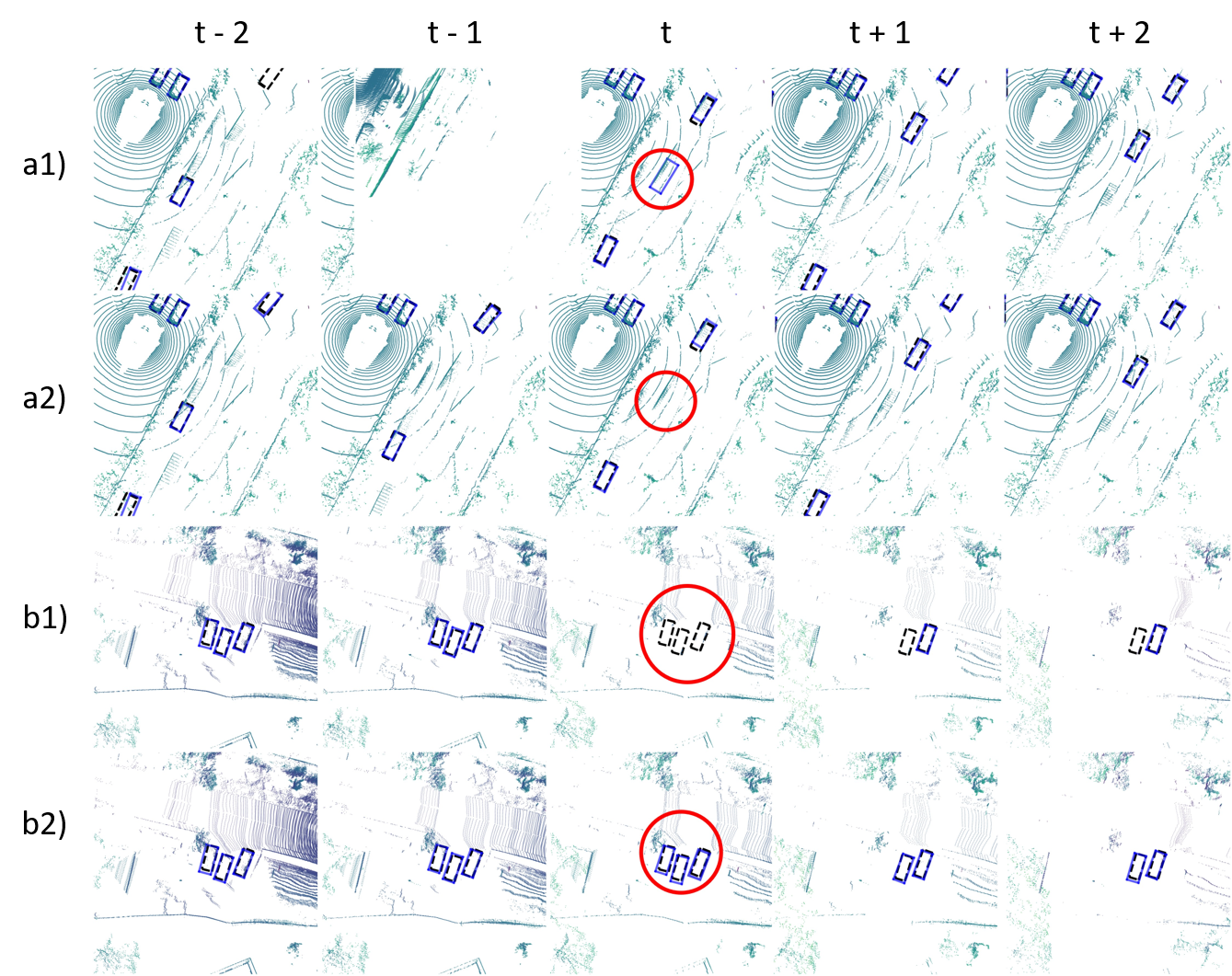
Figure 4: Qualitative Results: Ground truth detections are shown as black dashed boxes. Predicted detections are shown as blue boxes. We filter the detections with confidence lower than 0.5. The a1) and b1) show the detection results from initial student. The a2) and b2) rows show the result of our method. a2) shows our method successfully corrects false positive detections are near to high-scoring detections in adjacent frames (red circles). b2) shows our method corrects false negative detections that are isolated in time (red circles).

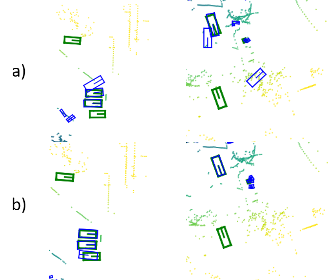
Figure 5: Qualitative Results (Semi-supervised): Ground truth detections are shown as green boxes. Predicted detections are shown as blue boxes. We filter the detections with confidence lower than 0.5. a) shows the results from the initial student. b) shows the result from the learned student. After training with unlabeled data via semi-supervised training, our method improves the detection results.

According to the ablation study, we show that each component contributes to the final improvement of the performance. Comparing the first and last row of Table 4, we prove using the tracking method instead the GNN model can get worse performance, because tracking method updates not only the confident score but also the position of each detected object. These object position predicted by Kalman Filter introduces new errors to the pseudo label, which are then learned by the student. Our (Flicker) indicates the GNN network of student can more efficient extract features and understand the relation among the objects from the point cloud video. Our (-Augmentations) shows the importance of graph augmentation for temporal GNN (comparing the third and last row of Table 4). The temporal GNN can easily overfit to the limited amount of labeled data without graph augmentation, and thus hurts the performance of the teacher and student. Our (-Gradually) indicates the importance of gradually training (comparing the fourth and last row of Table 4). Since the initial student is trained with limited label data, the model can easily get negative effect by large amount of pseudo labels with high uncertainty. Our (-Uncertainty) shows that even with spatiotemporal reasoning, the teacher’s prediction is still noisy. Thus using uncertainty to weight pseudo labels significantly reduce the affect of unreliable labels and thus can help the student to learn more from good samples. Our (-Iterative) shows that keeping the teacher updated is another key component to boost the detection performance as a better teacher can generate more reliable pseudo labels.

4.4 Qualitative Analysis

In this section, we qualitatively analyze our method. Figure 4 a1) and a2) visualizes examples where our method corrects false positive detections made by the original teacher. a1) shows the detection from initial student, where in frame $t$, ground-truth objects were failed to be detected. However, the detector is able to detect these objects in most of the previous two and next two frames. These are examples of “false positive flickers”, where a detection suddenly appears in one frame and disappears in the next. Since the GNN of student aggregates information from neighboring frames, it reasons that it is unlikely the object exists in frame $t$. Our method a2) successfully removes these false detections as shown in the second and fourth rows.

Similarly, Figure 4 b1) and b2) visualizes examples where the learned student corrects the initial teacher’s false negative. In the b1), the teacher falsely detects an object in frame $t$. However, most of the neighboring nodes do not have detections corresponding to this object. These are examples of “false negative flickers” where an object is predicted to disappear in one frame and immediately reappear in the next frame. Our method takes temporal information into account, and reasons that because the neighboring frames have positive detections at the same location, it is highly likely that there should be a detection in frame $t$. The b2) shows that our method increases the confidence of the flickered detections and correctly detects the missed objects.

Figure 5 shows the comparison between a) the initial teacher and b) the student trained by our proposed semi-supervised approach in two different scenarios. The detection from the pre-trained model with limited data shows lots of false positive and false negation. After feeding into more unlabeled data, the student network produces a more accurate detection results by learning both positive and negative sample with low uncertainty.

Overall, our approach combines the temporal information which reduces the uncertainty of pseudo labels and semi-supervised training pipeline which obtains the benefits from larger set of data to improve the generalization and robustness of the model.

5 Conclusion

In conclusion, we propose to leverage large amounts of unlabeled point cloud videos by semi-supervised learning of 3D object detectors via temporal graph neural networks. It does not require a large amount of strong labels that are often difficult to obtain. We show that teacher with temporal GNN can generate more accurate pseudo labels to train the student. By incorporating uncertainty-aware semi-supervised training, gradual semi-supervised training, and iterative refinement, our method achieves state-of-the-art detection performance on the challenging nuScenes [3] and H3D [19] benchmarks, compared to baselines trained on the same amount of labeled data. We hope that our work points toward moving away from spending excessive efforts annotating labeled data and instead redirecting them to semi-supervised learning on large unlabeled dataset.

Acknowledgements. The authors would like to thank members of R-pad for fruitful discussion and detailed feedback on the manuscript. Carnegie Mellon Effort has been supported by the Honda Research Institute USA, NSF S&AS Grant No. IIS-1849154.

References

- [1] Eric Arazo, Diego Ortego, Paul Albert, Noel E O’Connor, and Kevin McGuinness. Pseudo-labeling and confirmation bias in deep semi-supervised learning. In 2020 International Joint Conference on Neural Networks (IJCNN), pages 1–8. IEEE, 2020.
- [2] Linchao Bao, Baoyuan Wu, and Wei Liu. Cnn in mrf: Video object segmentation via inference in a cnn-based higher-order spatio-temporal mrf. In Proceedings of the IEEE conference on computer vision and pattern recognition, pages 5977–5986, 2018.
- [3] Holger Caesar, Varun Bankiti, Alex H Lang, Sourabh Vora, Venice Erin Liong, Qiang Xu, Anush Krishnan, Yu Pan, Giancarlo Baldan, and Oscar Beijbom. nuscenes: A multimodal dataset for autonomous driving. In Proceedings of the IEEE/CVF Conference on Computer Vision and Pattern Recognition, pages 11621–11631, 2020.
- [4] Andreas Geiger, Philip Lenz, Christoph Stiller, and Raquel Urtasun. Vision meets robotics: The kitti dataset. International Journal of Robotics Research (IJRR), 2013.
- [5] Ross Girshick. Fast r-cnn. In Proceedings of the IEEE international conference on computer vision, pages 1440–1448, 2015.
- [6] Ross Girshick, Jeff Donahue, Trevor Darrell, and Jitendra Malik. Rich feature hierarchies for accurate object detection and semantic segmentation. In Proceedings of the IEEE conference on computer vision and pattern recognition, pages 580–587, 2014.
- [7] Kaiming He, Georgia Gkioxari, Piotr Dollár, and Ross Girshick. Mask r-cnn. In Proceedings of the IEEE international conference on computer vision, pages 2961–2969, 2017.
- [8] Fa-Ting Hong, Wei-Hong Li, and Wei-Shi Zheng. Learning to detect important people in unlabelled images for semi-supervised important people detection. In Proceedings of the IEEE/CVF Conference on Computer Vision and Pattern Recognition, pages 4146–4154, 2020.
- [9] Rui Huang, Wanyue Zhang, Abhijit Kundu, Caroline Pantofaru, David A Ross, Thomas Funkhouser, and Alireza Fathi. An lstm approach to temporal 3d object detection in lidar point clouds. arXiv preprint arXiv:2007.12392, 2020.
- [10] SouYoung Jin, Aruni RoyChowdhury, Huaizu Jiang, Ashish Singh, Aditya Prasad, Deep Chakraborty, and Erik Learned-Miller. Unsupervised hard example mining from videos for improved object detection. In Proceedings of the European Conference on Computer Vision (ECCV), pages 307–324, 2018.
- [11] Diederik P Kingma and Jimmy Ba. Adam: A method for stochastic optimization. In ICLR (Poster), 2015.
- [12] Ananya Kumar, Tengyu Ma, and Percy Liang. Understanding self-training for gradual domain adaptation. In International Conference on Machine Learning, pages 5468–5479. PMLR, 2020.
- [13] Alex H Lang, Sourabh Vora, Holger Caesar, Lubing Zhou, Jiong Yang, and Oscar Beijbom. Pointpillars: Fast encoders for object detection from point clouds. In Proceedings of the IEEE Conference on Computer Vision and Pattern Recognition, pages 12697–12705, 2019.
- [14] Ming Liang, Bin Yang, Shenlong Wang, and Raquel Urtasun. Deep continuous fusion for multi-sensor 3d object detection. In Proceedings of the European Conference on Computer Vision (ECCV), pages 641–656, 2018.
- [15] Yen-Cheng Liu, Chih-Yao Ma, Zijian He, Chia-Wen Kuo, Kan Chen, Peizhao Zhang, Bichen Wu, Zsolt Kira, and Peter Vajda. Unbiased teacher for semi-supervised object detection. In Proceedings of the International Conference on Learning Representations (ICLR), 2021.
- [16] Xiankai Lu, Wenguan Wang, Martin Danelljan, Tianfei Zhou, Jianbing Shen, and Luc Van Gool. Video object segmentation with episodic graph memory networks. In Computer Vision–ECCV 2020: 16th European Conference, Glasgow, UK, August 23–28, 2020, Proceedings, Part III 16, pages 661–679. Springer, 2020.
- [17] Takeru Miyato, Shin-ichi Maeda, Masanori Koyama, and Shin Ishii. Virtual adversarial training: a regularization method for supervised and semi-supervised learning. IEEE transactions on pattern analysis and machine intelligence, 41(8):1979–1993, 2018.
- [18] David Nilsson and Cristian Sminchisescu. Semantic video segmentation by gated recurrent flow propagation. In Proceedings of the IEEE Conference on Computer Vision and Pattern Recognition (CVPR), June 2018.
- [19] Abhishek Patil, Srikanth Malla, Haiming Gang, and Yi-Ting Chen. The h3d dataset for full-surround 3d multi-object detection and tracking in crowded urban scenes. In International Conference on Robotics and Automation, 2019.
- [20] Federico Perazzi, Anna Khoreva, Rodrigo Benenson, Bernt Schiele, and Alexander Sorkine-Hornung. Learning video object segmentation from static images. In Proceedings of the IEEE conference on computer vision and pattern recognition, pages 2663–2672, 2017.
- [21] Hieu Pham, Qizhe Xie, Zihang Dai, and Quoc V Le. Meta pseudo labels. arXiv preprint arXiv:2003.10580, 2020.
- [22] Shaoqing Ren, Kaiming He, Ross Girshick, and Jian Sun. Faster r-cnn: Towards real-time object detection with region proposal networks. In Advances in neural information processing systems, pages 91–99, 2015.
- [23] Claude Elwood Shannon. A mathematical theory of communication. ACM SIGMOBILE mobile computing and communications review, 5(1):3–55, 2001.
- [24] Liyan Sun, Jianxiong Wu, Xinghao Ding, Yue Huang, Guisheng Wang, and Yizhou Yu. A teacher-student framework for semi-supervised medical image segmentation from mixed supervision. arXiv preprint arXiv:2010.12219, 2020.
- [25] Pei Sun, Henrik Kretzschmar, Xerxes Dotiwalla, Aurelien Chouard, Vijaysai Patnaik, Paul Tsui, James Guo, Yin Zhou, Yuning Chai, Benjamin Caine, et al. Scalability in perception for autonomous driving: Waymo open dataset. In Proceedings of the IEEE/CVF Conference on Computer Vision and Pattern Recognition, pages 2446–2454, 2020.
- [26] Alex Teichman and Sebastian Thrun. Tracking-based semi-supervised learning. The International Journal of Robotics Research, 31(7):804–818, 2012.
- [27] Sourabh Vora, Alex H Lang, Bassam Helou, and Oscar Beijbom. Pointpainting: Sequential fusion for 3d object detection. In Proceedings of the IEEE/CVF Conference on Computer Vision and Pattern Recognition, pages 4604–4612, 2020.
- [28] He Wang, Yezhen Cong, Or Litany, Yue Gao, and Leonidas J Guibas. 3dioumatch: Leveraging iou prediction for semi-supervised 3d object detection. In Proceedings of the IEEE/CVF Conference on Computer Vision and Pattern Recognition, pages 14615–14624, 2021.
- [29] Thomas Weng, Amith Pallankize, Yimin Tang, Oliver Kroemer, and David Held. Multi-modal transfer learning for grasping transparent and specular objects. IEEE Robotics and Automation Letters, 5(3):3791–3798, 2020.
- [30] Xinshuo Weng, Jianren Wang, David Held, and Kris Kitani. 3D Multi-Object Tracking: A Baseline and New Evaluation Metrics. IROS, 2020.
- [31] Chen Xia, Jianren Wang, David Held, and Martial Hebert. Panonet3d: Combining semantic and geometric understanding for lidarpoint cloud detection. In International Virtual Conference on 3D Vision (3DV), 2020.
- [32] Yu Xiang, Wonhui Kim, Wei Chen, Jingwei Ji, Christopher Choy, Hao Su, Roozbeh Mottaghi, Leonidas Guibas, and Silvio Savarese. Objectnet3d: A large scale database for 3d object recognition. In Bastian Leibe, Jiri Matas, Nicu Sebe, and Max Welling, editors, Computer Vision – ECCV 2016, pages 160–176, Cham, 2016. Springer International Publishing.
- [33] Qizhe Xie, Minh-Thang Luong, Eduard Hovy, and Quoc V Le. Self-training with noisy student improves imagenet classification. In Proceedings of the IEEE/CVF Conference on Computer Vision and Pattern Recognition, pages 10687–10698, 2020.
- [34] Yan Yan, Yuxing Mao, and Bo Li. Second: Sparsely embedded convolutional detection. Sensors, 18(10):3337, 2018.
- [35] Bin Yang, Wenjie Luo, and Raquel Urtasun. Pixor: Real-time 3d object detection from point clouds. In Proceedings of the IEEE conference on Computer Vision and Pattern Recognition, pages 7652–7660, 2018.
- [36] Xitong Yang, Xiaodong Yang, Ming-Yu Liu, Fanyi Xiao, Larry S Davis, and Jan Kautz. Step: Spatio-temporal progressive learning for video action detection. In Proceedings of the IEEE/CVF Conference on Computer Vision and Pattern Recognition, pages 264–272, 2019.
- [37] Junbo Yin, Jianbing Shen, Chenye Guan, Dingfu Zhou, and Ruigang Yang. Lidar-based online 3d video object detection with graph-based message passing and spatiotemporal transformer attention. In Proceedings of the IEEE/CVF Conference on Computer Vision and Pattern Recognition, pages 11495–11504, 2020.
- [38] Tianwei Yin, Xingyi Zhou, and Philipp Krähenbühl. Center-based 3d object detection and tracking. CVPR, 2021.
- [39] Bianca Zadrozny and Charles Elkan. Obtaining calibrated probability estimates from decision trees and naive bayesian classifiers. In Icml, volume 1, pages 609–616. Citeseer, 2001.
- [40] Na Zhao, Tat-Seng Chua, and Gim Hee Lee. Sess: Self-ensembling semi-supervised 3d object detection. In Proceedings of the IEEE/CVF Conference on Computer Vision and Pattern Recognition (CVPR), June 2020.
- [41] Yin Zhou and Oncel Tuzel. Voxelnet: End-to-end learning for point cloud based 3d object detection. In Proceedings of the IEEE Conference on Computer Vision and Pattern Recognition, pages 4490–4499, 2018.
- [42] Benjin Zhu, Zhengkai Jiang, Xiangxin Zhou, Zeming Li, and Gang Yu. Class-balanced grouping and sampling for point cloud 3d object detection. arXiv preprint arXiv:1908.09492, 2019.