Dilated Continuous Random Field for Semantic Segmentation
Abstract
Mean field approximation methodology has laid the foundation of modern Continuous Random Field (CRF) based solutions for the refinement of semantic segmentation. In this paper, we propose to relax the hard constraint of mean field approximation - minimizing the energy term of each node from probabilistic graphical model, by a global optimization with the proposed dilated sparse convolution module (DSConv). In addition, adaptive global average-pooling and adaptive global max-pooling are implemented as replacements of fully connected layers. In order to integrate DSConv, we design an end-to-end, time-efficient DilatedCRF pipeline. The unary energy term is derived either from pre-softmax and post-softmax features, or the predicted affordance map using a conventional classifier, making it easier to implement DilatedCRF for varieties of classifiers. We also present superior experimental results of proposed approach on the suction dataset comparing to other CRF-based approaches.
I INTRODUCTION
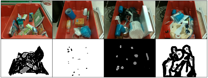
An affordance map indicates valid areas for suction-based bin-picking, ignored background, and negative samples that signify an object w/o valid suction areas, as shown in Fig. 1. The annotations are labeled by multiple human experts, which is not precise enough due to several reasons: the same object is annotated in various styles by different experts; annotations are yielded via seemingly paradoxical inferences, e.g., a glass is pickable while a plastic ball is not; some objects, such as a laser pen, or largely occluded objects, are labeled as pickable in some affordance maps, whereas being unpickable in others.
Therefore, the task to predict precise suction area is challenging given such conditions. No matter which approach is implemented to solve this challenging semantic segmentation task, the goal of CRF based post-processing is to refurbish the predictions into more fine-grained artifacts. As to the post-processing itself, real-time performance is preferred for robotic applications.
As one of the most popular works in demonstrating CRF for the field of semantic segmentation, the DenseCRF [1], proposes mean field approximation theory to approximate global energy minimization by optimizing local unary and pairwise potentials that encode relative positional and color information of entire image, and the message passing from other features to the local feature becomes the computational bottleneck, especially when the image is large in size. DenseCRF proposes to further boost the efficiency by lattice permutation [2], which reduces the computational complexity from to . Still, it remains to be a key topic seeking the perfect trade-off between better global approximation and efficiency.
In this paper, we investigate the implementation of standard convolution upon CRF, and decreasing the usage of fully-connect layers. It seems natural that single linear layer can learn relative relationship between a local feature and all other features by connecting all these features and output one pairwise energy term. Suppose a feature volume with a height and width of 60 and 80, this linear layer has a total trainable parameters of 4.8K. Consider all features of the feature volume, the total number of parameters is 23.04M, which will be subjected to quadratic growth if its height and width double. As a remedy to reduce total parameters, we propose the dilated sparse convolution (DSConv) module that performs fast channel-wise convolution with a static kernel, then extract global energy terms using adaptive global max pooling (AGMP) and adaptive global average pooling (AGAP) as replacements of linear layers. With DSConv modules, Dilated CRF decreases 23.04M parameters to 0.36M, while showing state-of-the-art performance.
DSConv module correlates features in a global manner other than following the mean field approximation methodology. Since DilatedCRF is end-to-end trained with a GPU, it can learn trainable parameters globally without customized CPU-only operations, e.g., the computation of potentials with L2-norms and convolution optimized by lattice permutation [1, 3], patch-wise multiplication [4], etc. Also, it should be noted that, the massive concatenation of output features, and memory transfer consume the majority of runtime. One of our future works is to accelerate these trivial operations.

II CONTINUOUS RANDOM FIELD
II-A The General Form
Suppose a label space , and are the height and width of the ground-truth, random variable , corresponds to a category of the suction dataset [5], and input feature volume , each is a 3-D feature vector. According to Hammersley-Clifford theorem, the CRF defined by and is then denoted as a Gibbs distribution over the set of all maximal cliques:
| (1) |
potential signifies a strict positive function defined on maximal clique of undirect graph . In the context of semantic segmentation, let be the set of all spatial locations, the edges that connect vertices from , then . is the normalization factor that ensures a valid probabilistic distribution,
| (2) |
CRF refinement is achieved by the maximum a posteriori (MAP) labeling w.r.t. ground-truth.
Complete graph is ideal for refinement. However, its defect is also noteworthy - massive computation to exhaustively enumerate all possible combinations of random variable . To avoid the prod operation, exponential function is applied to potentials such that
| (3) |
where the Gibbs energy . According to (3), optimization of a CRF can be denoted as , is ignored because it only depends on input feature volume .
II-B DenseCRF for Semantic Segmentation
Dense CRF employs a fully-connected graph such that there’s only one maximal clique. Let , the Gibbs energy has the form
| (4) |
where , are unary and pairwise potentials respectively. Commonly-implemented DenseCRF [1] defines as the output of a classifier given input , and as
| (5) |
where is the compatibility function which is manually assigned by Potts model , each is a learnable weight, and indicates a Gaussian kernel.
DenseCRF also approximates true distribution via mean field. It computes a distribution that minimize KL-divergence against , which takes the form
| (6) |
The assumption of mean field approximation is dedicate, that vertices of are conditional independent from each other. Therefore, minimizing the energy of each node results in an approximation of global minimum.
III RELATED WORKS
III-A Conventional CRF
Most of works on CRF are based on mean field approximation theory. For super-pixel image segmentation, Sulimowicz et al [7] formulate super-pixel cue onto pairwise potentials, which outperforms DenseCRF; Ma et al [8] introduce two coefficients to unary and pairwise potentials for better encoding super-pixel energy terms; Li et al [9] define a third potential to model the cost of assigning super-pixel labels; Yang et al [10] define a interlayer high order potential to enhance super-pixel segmentation. These works improve DenseCRF w/o adapting CRF to neural networks, which are categorized as conventional CRF.
III-B Refinement for Neural Networks
As a widely-applied refinement tool for CNN-based approaches, CRF has been proved to be effective in medical image segmentation, according to the references [11, 12, 13]. Lai et al [14] integrate DenseCRF into their DeepSqueezeNet for better performance. Zheng et al [15] present a fusion strategy of DenseCRF and attention module for unsupervised video object segmentation. Shimoda et al [16] compare their proposed approach with the refinement output of CRF, and come to the conclusion that their approach is superior, which indicates the failure of CRF in the processing of certain datasets.
III-C CRF as Neural Networks
Recently, several works emphasize on the possibilities of adapting CRF to neural network. CRF-RNN [3] is the first architecture that trains a DenseCRF end-to-end via Convolutional Neural Network (CNN) and Recurrent Neural Network (RNN). This work breaks down DenseCRF to common CNN operations except the lattice permutation during message passing of pairwise energy term, and trains these operations iteratively as a RNN. Vemulapalli et al [17] propose the Gaussian mean field approximation that computes pairwise energy into three steps - a CNN to generate features, a similarity layer that computes similarity scores, and a matrix generation layer that compute Gaussian weights. Although CNN is well-integrated into the GaussianCRF pairwise energy term, the Gaussian filtering process requires non-standard neural network operations.
Another variant is to compute CRF as a CNN. Teichmann and Cipolla [4] design a ConvCRF that constraints the fully-connected computational graph into locally-connected blocks via Manhattan distance, which greatly boosts the efficiency of message passing process with the cost of losing long-range connections. Nguyen et al [18] take the advantages of Gated Recurrent Unit [19] (GRU), reformulating CRF-RNN as CRF-GRU that avoids the gradient vanishing and exploding problem of RNN. The gated architecture also enables CRF-GRU to model long-term relationships. Lin et al [20] propose to learn unary and pairwise energies via fully-connected layers from node and edge feature vectors that are yielded from a manually-constructed CRF graph and a convolutional network.
IV METHODOLOGY
IV-A Dilated CRF
Proposed DilatedCRF reformulates Gibbs energy term as fully-learnable unary and global potential444Note that is not finalized by an activation function after the weighted sum operation. :
| (7) |
In (7), , is a weights vector with the same length as , which learns the unary term in (4). Particularly, is the raw input affordance map, which can either be the artifacts after final softmax layer, or the output using conventional classifiers such as random forest [21]. Unary potential , global potentials and can be optimized iteratively during training. is defined as
| (8) |
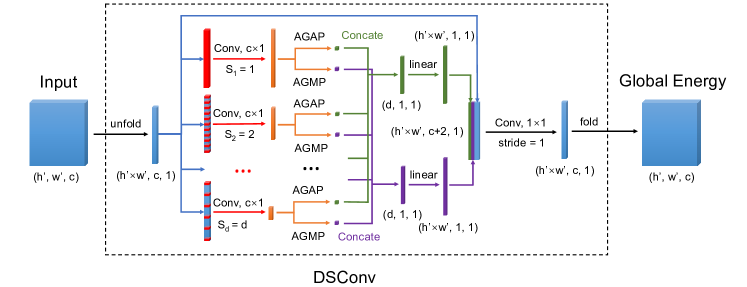
where is a trainable weights matrix that up-samples global feature to desired length . Moreover, learns the mapping from to potential which is not necessarily a valid probability distribution. Follow the DSConv architecture shown in Fig. 3, let be the total number of convolution kernels, and -th kernel has a convolutional stride of , define as the length of output feature, we have
| (9) |
| (10) |
the operator signifies the height-wise concatenation of elements. DilatedCRF is trained end-to-end to minimize KL-Divergence between and the ground-truth. All weights are learnable through gradients back-propagation since (7) - (10) are differential.
IV-B Architecture
Fig. 3 illustrates standard operations to perform DilatedCRF inference. We implement a fractional max-pooling [22] layer to down-sample the input label, and nearest interpolation to up-sample refined feature maps. Each channel of the 3-channels unary energy term is computed via convolution and batch normalization (BN) layer.
The main contribution of this paper is the DSConv module that encodes the short-term and long-term relationship between feature vectors. As shown in Fig. 3, input feature volume is unfolded into a long vector with the shape of , sparse convolution using static kernel filtering has strides to perform global correlations, which, in our experiment, we let for octant-size, quarter-size, half-size, and 10 for full-size DilatedCRFs. The AGAP operation (refer to (9)) computes average energy intensity, and AGMP operation (refer to (10)) locates the strongest response for feature . Both features effectively encode the contribution of with less parameters than that of implementing two independent linear layers. Additionally, raw input feature is concatenated with the average global feature and maximal global feature for the purpose of reusing features and alleviating the vanishment of gradients. The linear up-sampling operation is based on (8), which is the most critical procedure to learn the relation between and . Equation (7) is realized by performing convolution upon concatenated features.
| Items | Full-Size | Half-Size | Quarter-Size | Octant-Size | LR-ASPP [23] |
|---|---|---|---|---|---|
| Total parameters (M) | 0.09 | 21.66 | 2.77 | 0.36 | - |
| Inference time (ms) | 13.99 | 159.43 | 18.81 | 8.91 | - |
| Accuracy (%) | 96.56 2.76 | 96.22 2.76 | 96.35 2.78 | 96.29 2.71 | 96.61 2.80 |
| Jaccard Index (%) | 40.75 23.42 | 40.77 23.20 | 41.21 23.30 | 39.84 22.67 | 40.07 23.72 |
| Precision (%) | 57.37 28.12 | 53.09 27.68 | 54.30 27.58 | 54.67 28.23 | 58.16 28.20 |
| Recall (%) | 58.47 24.78 | 64.42 23.74 | 62.84 23.85 | 61.11 23.17 | 56.02 25.76 |
| Dice Coefficient (%) | 53.94 24.24 | 54.03 24.01 | 54.45 24.08 | 53.20 23.69 | 53.07 24.86 |
IV-C Training
Assume the true conditional probability distribution of ground-truth is denoted as , KL-Divergence is calculated by
| (11) |
If is one-hot encoded, KL-Divergence equals the value of cross-entropy loss (CELoss), we thereby utilize a weighted form of CELoss function for training DilatedCRF:
| (12) |
where is a manually-set weight for the category , and the subscript variable indicates a category of {‘background’, ‘negative samples’, ‘valid suckable area’}.
We trained the network by setting to (0.25, 0.25, 0.5), the weight assigned for category 2 is larger than other weights because the valid suckable regions usually occupy a small portion of the image, while we only need to evaluate this category. The suction dataset [5] has a training split of 1470 images, and a testing split of 367 images, each image has a resolution of 480640.
V EXPERIMENTS
V-A Implementation Details
V-A1 Training and test
We follow a four-stages strategy to train and test DilatedCRF w/ a RTX3080 GPU:
-
•
Pre-train classifiers on the training set.
-
•
Generate predicated post-softmax555Alternatively, pre-softmax affordance maps are also theoretically valid. affordance maps for both training and test sets.
-
•
Train DilatedCRF using the predicted affordance maps w/ AdamW optimizer (w/o weight decay) and a learning rate of 1.
-
•
Test the DilatedCRF using a selected checkpoint, and evaluate results by segmentation metrics.
Typically, it takes around 5 hours to train a half-size DilatedCRF. We quantitatively evaluate the results by Jaccard Index, Precision, Recall, Dice coefficient, and Accuracy, which are defined as
| (13) |
| (14) |
| (15) |
| (16) |
V-A2 Performance in Training
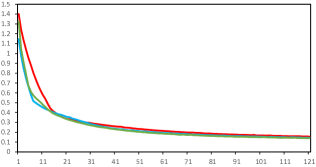
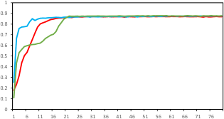
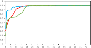
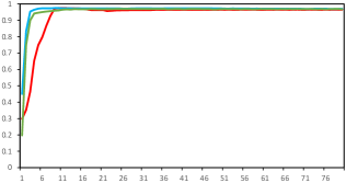
In Fig. 4, we report more training details for half-size, quarter-size and octant-size DilatedCRFs. Over-fitting is not observed as loss curves (in Fig. 4a) converge at around 0.11, and curves of metrics arrive at their maximums before the convergence.
It can also be inferred from Fig. 4b-4d that quarter-size DilatedCRF manifests the fastest convergence speed during training, and Jaccard Index curves behaves extremely similar to precision curves, which indicates precision is more decisive than recall for the suction dataset. Although differ in sizes, all three models converge to the same numerical level upon the training set.
| Items | ConvCRF | DenseCRF |
|---|---|---|
| Inference time (ms) | 14.10 | 450.16 |
| Accuracy (%) | 96.40 2.84 | 96.74 2.89 |
| Jaccard Index (%) | 34.35 22.95 | 33.76 25.63 |
| Precision (%) | 54.23 29.17 | 60.49 32.35 |
| Recall (%) | 48.76 28.43 | 43.31 30.74 |
| Dice Coefficient (%) | 46.77 25.94 | 45.05 28.75 |
V-A3 Test performance
As shown in Tab. I, all DilateCRFs outperform the original LR-ASPP [23] approach on Recall and Dice scores, which indicates the potential of DilatedCRF in locating more objects, while maintaining high precision and lower uncertainties manifested by standard deviation. Octant-size DilatedCRF has the coarsest affordance predictions for the 8 lower down-sampling, however, it shows competitive performance both in Accuracy and Jaccard Index, and only takes additional 9ms inference runtime for refinement. The quarter-size DilatedCRF performs the best among all DilatedCRFs considering the trade-off between inference time and all metrics. Furthermore, it achieves the highest Dice score. Half-size DilatedCRFs continue to robustly improve Recall score whereas the twofold enlargements of image height and width greatly slows down inference procedure, bringing in more noisy features. For full-size DilatedCRF w/o the down-sampling and up-sampling layers shown in Fig. 3, coefficient is set to 10, which dramatically boosts the runtime efficiency.
V-B Compare to other CRFs
In this section, we report our quantitative and qualitative results with ConvCRF [4] and DenseCRF [1]. ConvCRF is tested w/ a RTX3080 GPU, and DenseCRF is tested w/ a 3.60GHz Intel i9-10850K CPU.
V-B1 Quantitative Evaluation
As shown in Tab. II, DenseCRF achieves the highest average precision and accuracy among all tested approaches. However, due to the largest variances, DenseCRF does not perform as stably as desired. Also, its lower recall and Jaccard index significantly degrade its performance on test set. ConvCRF, in the other hand, make a relatively better trade-off between recall and precision. It is noteworthy that, although ConvCRF has an average performance, it runs 32 faster than DenseCRF.
V-B2 Qualitative Results
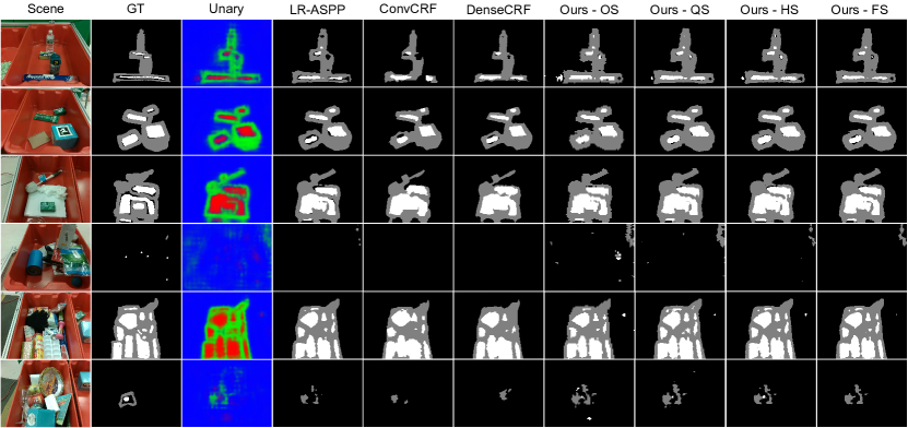
Fig. 5 depicts affordance maps, images of scenes, and post-softmax unary maps. Both ConvCRF and DenseCRF enhance boundaries better than neural network based approaches. Nonetheless, the defects of these two approaches are obvious. First, they tend to filter out small regions, which may lower the success rate of suction-type picking. Second, the relationships between separated regions may not being well-encoded due to the chromatic continuities of raw scenes, which results in largely-connected affordance maps.
In comparison with ConvCRF and DenseCRF, the proposed approaches better recognize the relationships between separated regions, and locate more objects whereas some of them are not from the ground-truth. Although these predictions are categorized as false negatives, as depicted in Fig. 5, a robotic hand may successfully pick an object from bins under the guidance of these predictions. Generally, the proposed approaches directly learn vanilla features from unary maps, progressively refine memorized features towards the ground-truth. Furthermore, we test the checkpoint after 200 epoches, and discover a similar performing trend as of DenseCRF, i.e., higher accuracy and precision but lower recall and Jaccard index than LR-ASPP artifacts, which indicates the potential of DSConv module to approximate the global optimum of fully-connect CRF.
VI CONCLUSION AND FUTURE WORKS
We propose DilatedCRF to approximate fully-connected CRF without relying on mean-field approximation. DilatedCRF reformulate unary and pairwise energy terms as learnable unary and global energy terms. The reformulation adapts the end-to-end neural networks to conventional CRF without CPU-only operations, which is faster and more liable for real-world implementations. To realize this reformulation, we design a dilated sparse convolution module that takes advantages of adaptive global average-pooling and adaptive global max-pooling, as well as the 3-stages DilatedCRF pipeline to accommodate varieties of unary maps. Extensive experimental results show the high efficiency, and competitive performance of the DilateCRF pipeline for realtime robotic suction-type bin-picking.
Our future works include:
-
•
Apply highly-precise backbone networks to better learn the unary terms.
-
•
Use network adaptive searching strategies to find the best strides for DSConv module.
-
•
Integrate high-order contextual information into global energy terms, this may further enhance the regional encoding capabilities of DilatedCRF.
-
•
Speed up the inferential procedures of full-size and half-size models by reducing concatenation operations.
ACKNOWLEDGMENT
We thank Li, Rui for the sponsorship of NVIDIA GPUs and INTEL CPUs, and M. Teichmann, R. Cipolla for providing open source codes of their [4] invaluable works.
References
- [1] P. Krähenbühl and V. Koltun, “Efficient inference in fully connected crfs with gaussian edge potentials,” Advances in neural information processing systems, vol. 24, pp. 109–117, 2011.
- [2] A. Adams, J. Baek, and M. A. Davis, “Fast high-dimensional filtering using the permutohedral lattice,” in Computer Graphics Forum, vol. 29, no. 2, 2010, pp. 753–762.
- [3] S. Zheng, S. Jayasumana, B. Romera-Paredes, V. Vineet, Z. Su, D. Du, C. Huang, and P. H. Torr, “Conditional random fields as recurrent neural networks,” in International Conference on Computer Vision, 2015, pp. 1529–1537.
- [4] M. Teichmann and R. Cipolla, “Convolutional crfs for semantic segmentation,” in British Machine Vision Conference, 2019.
- [5] A. Zeng, “Dataset,” https://vision.princeton.edu/projects/2017/arc/, Mar. 2018, accessed 6/27/2021.
- [6] J. L. Ba, J. R. Kiros, and G. E. Hinton, “Layer normalization,” Stat, vol. 1050, p. 21, 2016.
- [7] L. Sulimowicz, I. Ahmad, and A. Aved, “Superpixel-enhanced pairwise conditional random field for semantic segmentation,” in International Conference on Image Processing, 2018, pp. 271–275.
- [8] F. Ma, F. Gao, J. Sun, H. Zhou, and A. Hussain, “Weakly supervised segmentation of sar imagery using superpixel and hierarchically adversarial crf,” Remote Sensing, vol. 11, no. 5, p. 512, 2019.
- [9] Y. Li, Y. Liu, G. Liu, and M. Guo, “Weakly supervised semantic segmentation by iterative superpixel-crf refinement with initial clues guiding,” Neurocomputing, vol. 391, pp. 25–41, 2020.
- [10] Y. Yang, A. Stein, V. A. Tolpekin, and Y. Zhang, “High-resolution remote sensing image classification using associative hierarchical crf considering segmentation quality,” Geoscience and Remote Sensing Letters, vol. 15, no. 5, pp. 754–758, 2018.
- [11] J. Zhang, C. Li, F. Kulwa, X. Zhao, C. Sun, Z. Li, T. Jiang, H. Li, and S. Qi, “A multiscale cnn-crf framework for environmental microorganism image segmentation,” BioMed Research International, vol. 2020, 2020.
- [12] W. Luo and M. Yang, “Fast skin lesion segmentation via fully convolutional network with residual architecture and crf,” in International Conference on Pattern Recognition, 2018, pp. 1438–1443.
- [13] W. Deng, Q. Shi, M. Wang, B. Zheng, and N. Ning, “Deep learning-based hcnn and crf-rrnn model for brain tumor segmentation,” IEEE Access, vol. 8, pp. 26 665–26 675, 2020.
- [14] D. Lai, Y. Deng, and L. Chen, “Deepsqueezenet-crf: A lightweight deep model for semantic image segmentation,” in International Joint Conference on Neural Networks, 2019, pp. 1–8.
- [15] M. Zhen, S. Li, L. Zhou, J. Shang, H. Feng, T. Fang, and L. Quan, “Learning discriminative feature with crf for unsupervised video object segmentation,” in European Conference on Computer Vision, 2020, pp. 445–462.
- [16] W. Shimoda and K. Yanai, “Self-supervised difference detection for weakly-supervised semantic segmentation,” in International Conference on Computer Vision, 2019, pp. 5208–5217.
- [17] R. Vemulapalli, O. Tuzel, M.-Y. Liu, and R. Chellapa, “Gaussian conditional random field network for semantic segmentation,” in Computer Vision and Pattern Recognition, 2016, pp. 3224–3233.
- [18] K. Nguyen, C. Fookes, and S. Sridharan, “Context from within: Hierarchical context modeling for semantic segmentation,” Pattern Recognition, vol. 105, p. 107358, 2020.
- [19] K. Cho, B. van Merrienboer, C. Gulcehre, F. Bougares, H. Schwenk, and Y. Bengio, “Learning phrase representations using rnn encoder-decoder for statistical machine translation,” in Conference on Empirical Methods in Natural Language Processing, 2014.
- [20] G. Lin, C. Shen, A. Van Den Hengel, and I. Reid, “Efficient piecewise training of deep structured models for semantic segmentation,” in Computer Vision and Pattern Recognition, 2016, pp. 3194–3203.
- [21] M. Y. Yang and W. Förstner, “A hierarchical conditional random field model for labeling and classifying images of man-made scenes,” in International Conference on Computer Vision Workshops, 2011, pp. 196–203.
- [22] B. Graham, “Fractional max-pooling,” arXiv:1412.6071, 2014.
- [23] A. Howard, M. Sandler, G. Chu, L.-C. Chen, B. Chen, M. Tan, W. Wang, Y. Zhu, R. Pang, V. Vasudevan, et al., “Searching for mobilenetv3,” in International Conference on Computer Vision, 2019, pp. 1314–1324.