Calibration of P-values for calibration and for deviation of a subpopulation from the full population

Abstract

The author’s recent research papers, “Cumulative deviation of a subpopulation from the full population” and “A graphical method of cumulative differences between two subpopulations” (both published in volume 8 of Springer’s open-access Journal of Big Data during 2021), propose graphical methods and summary statistics, without extensively calibrating formal significance tests. The summary metrics and methods can measure the calibration of probabilistic predictions and can assess differences in responses between a subpopulation and the full population while controlling for a covariate or score via conditioning on it. These recently published papers construct significance tests based on the scalar summary statistics, but only sketch how to calibrate the attained significance levels (also known as “P-values”) for the tests. The present article reviews and synthesizes work spanning many decades in order to detail how to calibrate the P-values. The present paper presents computationally efficient, easily implemented numerical methods for evaluating properly calibrated P-values, together with rigorous mathematical proofs guaranteeing their accuracy, and illustrates and validates the methods with open-source software and numerical examples.

Keywords: Brownian motion, significance, test, hypothesis, numerical methods, graph

1 Introduction

Two basic problems in statistics are (1) checking calibration of probabilistic predictions such that any event predicted to happen, say, $x$ percent of the time actually occurs $x$ percent of the time and (2) assessing the deviation of a subpopulation from the full population while conditioning on a specified covariate or score (“conditioning on” is also known as “controlling for,” and involves comparing only individuals whose values for the covariate or score are similar or otherwise match up). In fact, the first problem can be viewed as a special case of the second problem by requiring the expected response of the full population to be equal to the predicted probability, so that the deviation of the subpopulation from the full population is simply the deviation from the probabilities. In all cases, the data consists of observations of responses paired with scores (and weights, in the case of weighted samples). In the first case, the scores are the predicted probabilities; in the second case, the scores are the values of the specified covariate (which could be probabilistic predictions, too). In the social and biomedical sciences, controlling for income or age is common.

Recent work of Tygert (2021a) and Tygert (2021b) proposes metrics for (inter alia) measuring miscalibration or deviation of a subpopulation from the full population, reviewed in Subsection 2.2 below. The present paper develops methods for converting the values of such metrics into properly calibrated attained significance levels (also known as “P-values”), deriving the cumulative distribution functions for the metrics under the null hypothesis of no deviation between the subpopulation and the full population (or of perfect calibration in the underlying subpopulation). As reviewed below, the works of Delgado (1993), Diebolt (1995), and Stute (1997) prove that the estimates at finite sample sizes converge reasonably rapidly to the limiting asymptotic values in most settings encountered in practice, as confirmed in the numerical experiments presented below. Figures 4 and 5 below illustrate the rapid convergence. The metrics discussed in the present paper are very similar to those of Kuiper (1962) and of Kolmogorov (1933) and Smirnov (1939).

The earlier works broke ties in the scores at random, randomly ordering observations corresponding to exactly the same score. Subsection 2.4 below proposes an alternative that avoids any randomization (though randomization does simplify the analysis a bit). Subsection 2.4’s new approach may be of interest beyond just for the calibration of P-values.

The present paper carefully elaborates on widely deployed prior work, elucidating many details that earlier publications omitted. The elaboration is for the convenience and reference of the reader; the reader undoubtedly could derive most of the results presented below, but is welcome to spare the extensive effort required by instead leveraging the present paper and the associated open-source software. The presentation below provides full proofs that earlier publications omitted, and also summarizes everything required to solve the problems posed here, rather than requiring the reader to traverse literature that spans many decades and disciplines. The present paper is a response to many requests for pulling together everything into a comprehensive, convenient, reasonably elementary exposition, as well as elaborating the simple approach of Subsection 2.4 that not every (any?) end-user had realized was possible. In particular, Subsection 2.2 below briefly reviews the cumulative methods of Tygert (2021a) for assessing the deviation of a subpopulation from the full population; readers unfamiliar with that approach may wish to start with the full paper of Tygert (2021a) or the summary in Subsection 2.2 below.

The remainder of the paper has the following structure: Section 2 presents the main methods, Section 3 validates and illustrates the methods via numerical examples, and Section 4 briefly discusses the results and draws conclusions.

2 Methods

The present section details the methodology of the present paper. Subsection 2.1 provides computationally efficient formulae for evaluating the cumulative distribution functions of the range and of the maximum absolute value of the standard Brownian motion over the unit interval $[0,1]$, based on the works of Feller (1951) and Darling and Siegert (1953). Subsection 2.2 reviews the methods of Tygert (2021a) for assessing deviation of a subpopulation from the full population and for assessing calibration of probabilistic predictions, introducing a graphical method along with two statistics which summarize the graph as scalars. Next, Subsection 2.3 shows how to use the numerical methods of Subsection 2.1 to calculate attained significance levels (P-values) for the scalar summary statistics introduced in Subsection 2.2, based on the works of Delgado (1993), Diebolt (1995), and Stute (1997). Finally, Subsection 2.4 explains an alternative to breaking ties in the covariates or scores at random (randomization does simplify the analysis slightly, but avoiding randomization altogether is possible, too). Readers unfamiliar with the work of Tygert (2021a) or Tygert (2021b) might want to skip to Subsection 2.2 at first; however, readers interested mainly in the numerical methods might want to start instead with Subsection 2.1.

2.1 Distributions of the range and maximum absolute value of Brownian motion

This subsection presents series for the cumulative distribution functions of the range and maximum absolute value of the standard Brownian motion over the unit interval $[0,1]$. The terms in the series consist entirely of elementary functions that are easy to program (as implemented in the codes mentioned in Section 3). The series converge rapidly and the present subsection proves rigorous bounds on the numbers of terms required to attain a specified accuracy. Subsubsection 2.1.1 gives the results for the range of the standard Brownian motion — see especially Theorems 3 and 4; Subsubsection 2.1.2 gives the results for the maximum absolute value — see Theorems 5 and 6.

2.1.1 Range of the standard Brownian motion

This subsubsection presents Theorems 3 and 4, enabling easy, rapid computation of the cumulative distribution function for the range (the maximum minus the minimum) of the standard Brownian motion over the unit interval $[0,1]$.

We define the series

$$F(x)=\sum_{k=1}^{\infty}\left(\frac{8}{x^{2}}+\frac{8}{(2k-1)^{2}\pi^{2}}\right)\exp\left(-\frac{(2k-1)^{2}\pi^{2}}{2x^{2}}\right)$$ (1)

for any positive real number $x$. The following theorem exhibits $F$ to be the cumulative distribution function associated with the probability density function of Formulae 3.6–3.8 of Feller (1951); Theorem 2 below reviews those formulae.

Theorem 1.

Suppose that $F$ is the series defined in (1). Then,

$$F(x)=\int_{0}^{x}f(y)\,dy$$ (2)

for any positive real number $x$, where

$$f(x)=\sqrt{\frac{2}{\pi x^{2}}}\;\cdot\;\frac{\partial G}{\partial x}\left(\frac{x}{2}\right),$$ (3)

with

$$G(x)=\frac{\sqrt{2\pi}}{x}\sum_{k=1}^{\infty}\exp\left(-\frac{(2k-1)^{2}\pi^{2}}{8x^{2}}\right).$$ (4)

Proof.

Clearly $\lim_{x\to 0^{+}}F(x)=0=\lim_{x\to 0^{+}}\int_{0}^{x}f(y)\,dy$, so we need only show that $\frac{\partial F}{\partial x}=f$.

Differentiating (4) yields

$$\sqrt{\frac{2}{\pi}}\;\cdot\;\frac{\partial G}{\partial x}=\sum_{k=1}^{\infty}\left(\frac{2}{x}\frac{(2k-1)^{2}\pi^{2}}{4x^{3}}-\frac{2}{x^{2}}\right)\exp\left(-\frac{(2k-1)^{2}\pi^{2}}{8x^{2}}\right),$$ (5)

which when combined with (3) yields

$$f(x)=\sum_{k=1}^{\infty}\left(\frac{8(2k-1)^{2}\pi^{2}}{x^{5}}-\frac{8}{x^{3}}\right)\exp\left(-\frac{(2k-1)^{2}\pi^{2}}{2x^{2}}\right).$$ (6)

Differentiating (1) yields

$$\frac{\partial F}{\partial x}=\sum_{k=1}^{\infty}\left[\left(\frac{8}{x^{2}}+\frac{8}{(2k-1)^{2}\pi^{2}}\right)\left(\frac{(2k-1)^{2}\pi^{2}}{x^{3}}\right)-\frac{16}{x^{3}}\right]\exp\left(-\frac{(2k-1)^{2}\pi^{2}}{2x^{2}}\right)$$ (7)

The right-hand sides of (6) and (7) are equal, completing the proof. ∎

Formulae 3.6–3.8 of Feller (1951) state the following theorem, though Formula 3.6 of Feller (1951) is missing a factor of $1/\sqrt{t}$.

Theorem 2.

The probability density function for the range of the standard Brownian motion over the unit interval $[0,1]$ is given by Formula (3). (The range is the maximum minus the minimum.)

Combining Theorems 1 and 2 yields the following theorem.

Theorem 3.

The cumulative distribution function for the range (the maximum minus the minimum) of the standard Brownian motion over the unit interval $[0,1]$ is given by Formula (1).

The following theorem upper-bounds the tail of the series for $F$ defined in (1).

Theorem 4.

Suppose that $n$ is a positive integer. Then, the tail of the series for $F$ defined in (1) satisfies

$$\sum_{k=n+1}^{\infty}\left(\frac{8}{x^{2}}+\frac{8}{(2k-1)^{2}\pi^{2}}\right)\exp\left(-\frac{(2k-1)^{2}\pi^{2}}{2x^{2}}\right)<\frac{4}{\sqrt{2\pi}}\left(\frac{1}{x}+\frac{x}{\pi^{2}}\right)\exp\left(-\frac{(2n-1)^{2}\pi^{2}}{2x^{2}}\right)$$ (8)

for any positive real number $x$. If $\varepsilon$ is a positive real number less than 1 and

$$n\geq\frac{1}{2}+\frac{x}{\pi\sqrt{2}}\sqrt{\ln\left(\frac{4}{\varepsilon\sqrt{2\pi}}\left(\frac{1}{x}+\frac{x}{\pi^{2}}\right)\right)},$$ (9)

then the right-hand side of (8) is at most $\varepsilon$.

Proof.

Clearly,

$$\sum_{k=n+1}^{\infty}\!\left(\frac{8}{x^{2}}+\frac{8}{(2k-1)^{2}\pi^{2}}\right)\exp\left(-\frac{(2k-1)^{2}\pi^{2}}{2x^{2}}\right)<\left(\frac{8}{x^{2}}+\frac{8}{\pi^{2}}\right)\sum_{k=n+1}^{\infty}\!\exp\left(-\frac{(2k-1)^{2}\pi^{2}}{2x^{2}}\right)\!,$$ (10)

$$\sum_{k=n+1}^{\infty}\exp\left(-\frac{(2k-1)^{2}\pi^{2}}{2x^{2}}\right)<\int_{n}^{\infty}\exp\left(-\frac{(2t-1)^{2}\pi^{2}}{2x^{2}}\right)\,dt,$$ (11)

$$\int_{n}^{\infty}\exp\left(-\frac{(2t-1)^{2}\pi^{2}}{2x^{2}}\right)\,dt=\frac{x}{\pi\sqrt{2}}\int_{((2n-1)\pi)/(x\sqrt{2})}^{\infty}\exp(-u^{2})\,du,$$ (12)

and

$$\int_{\frac{(2n-1)\pi}{x\sqrt{2}}}^{\infty}\exp(-u^{2})\,du\leq\exp\left(-\frac{(2n-1)^{2}\pi^{2}}{2x^{2}}\right)\int_{0}^{\infty}\!\exp(-u^{2})\,du=\frac{\sqrt{\pi}}{2}\exp\left(-\frac{(2n-1)^{2}\pi^{2}}{2x^{2}}\right)\!.$$ (13)

Combining (10)–(13) yields (8). ∎

2.1.2 Maximum absolute value of the standard Brownian motion

This subsubsection presents Theorems 5 and 6, enabling easy, rapid computation of the cumulative distribution function for the maximum of the absolute value of the standard Brownian motion over the unit interval $[0,1]$.

The following theorem states Formulae 3.8 and 5.2 of Darling and Siegert (1953); see also the displayed formula immediately before Formula 5.2 of Darling and Siegert (1953), or Formula 2.22 of Ciesielski and Taylor (1962) and the sentence of Ciesielski and Taylor (1962) immediately following.

Theorem 5.

The cumulative distribution function for the maximum of the absolute value of the standard Brownian motion over the unit interval $[0,1]$ is

$$D(x)=\frac{4}{\pi}\sum_{k=1}^{\infty}\frac{(-1)^{k-1}}{2k-1}\exp\left(-\frac{(2k-1)^{2}\pi^{2}}{8x^{2}}\right)$$ (14)

for any positive real number $x$.

The following theorem follows from the Leibniz bound on the tail of an alternating series for which the absolute values of the terms in the series decrease monotonically to zero (namely, the absolute value of the leading term of the tail is an upper bound on the absolute value of the tail; the bound in Theorem 6 would also be valid if the summation started from $n$ rather than $n+1$).

Theorem 6.

Suppose that $n$ is a positive integer. Then, the tail of the series for $D$ defined in (14) satisfies

$$\left|\frac{4}{\pi}\sum_{k=n+1}^{\infty}\frac{(-1)^{k-1}}{2k-1}\exp\left(-\frac{(2k-1)^{2}\pi^{2}}{8x^{2}}\right)\right|<\frac{4}{\pi}\exp\left(-\frac{(2n-1)^{2}\pi^{2}}{8x^{2}}\right)$$ (15)

for any positive real number $x$. If $\varepsilon$ is a positive real number less than 1 and

$$n\geq\frac{1}{2}+\frac{x\sqrt{2}}{\pi}\sqrt{\ln\left(\frac{4}{\pi\varepsilon}\right)},$$ (16)

then the right-hand side of (15) is at most $\varepsilon$.

2.2 Calibration and deviation of a subpopulation from the full population

This subsection summarizes methods of Tygert (2021a) for assessing deviation of a subpopulation from the full population and for assessing the calibration of probabilistic predictions. The primary goal of this subsection is to introduce the Kolmogorov-Smirnov and Kuiper metrics, as well as factors suitable for normalizing them so as to facilitate evaluation of attained significance levels (P-values).

We consider $n$ real numbers $S_{1}$, $S_{2}$, …, $S_{n}$ known as “scores” (or sometimes as “predicted probabilities” when calibrating probabilistic predictions), each paired with a real-valued “response,” $R_{1}$, $R_{2}$, …, $R_{n}$, as well as a positive “weight,” $W_{1}$, $W_{2}$, …, $W_{n}$; we view the scores $S_{1}$, $S_{2}$, …, $S_{n}$ and weights $W_{1}$, $W_{2}$, …, $W_{n}$ as given, not random, while we view the responses $R_{1}$, $R_{2}$, …, $R_{n}$ as random. We assume throughout that all responses are stochastically independent (allowing dependence among the responses would be far beyond the scope of the present paper). Without loss of generality, we assume that $S_{1}<S_{2}<\dots<S_{n}$ (perturbing the original scores slightly in order to ensure their uniqueness, if necessary). We consider also a given function $r$ which returns the expected response averaged over the full population at any specified score $s$; that is, $r(s)$ is the expected value of the response for all members of the full population whose score is $s$. When assessing the calibration of probabilistic predictions, the score $s$ is a predicted probability and the expected response $r(s)$ is supposed to match the prediction, $s$; hence, $r(s)=s$ when assessing calibration.

In order to gauge deviation of the observed responses $R_{1}$, $R_{2}$, …, $R_{n}$ from the given function $r$, we construct the sequence of cumulative differences

$$B_{\ell}=\frac{\sum_{k=1}^{\ell}(R_{k}-r(S_{k}))\,W_{k}}{\sum_{k=1}^{n}W_{k}}$$ (17)

for $\ell=1$, $2$, …, $n$. We also construct the sequence of cumulative weights

$$A_{\ell}=\frac{\sum_{k=1}^{\ell}W_{k}}{\sum_{k=1}^{n}W_{k}}$$ (18)

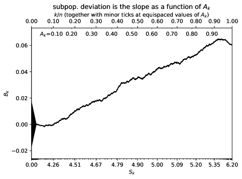
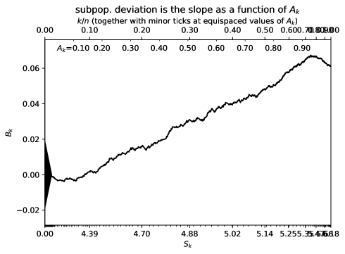
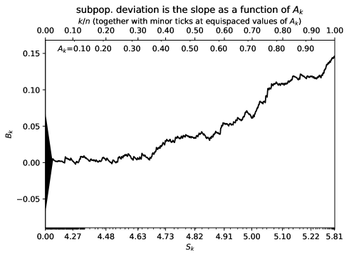
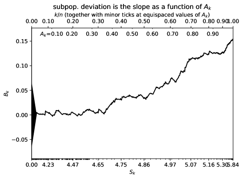
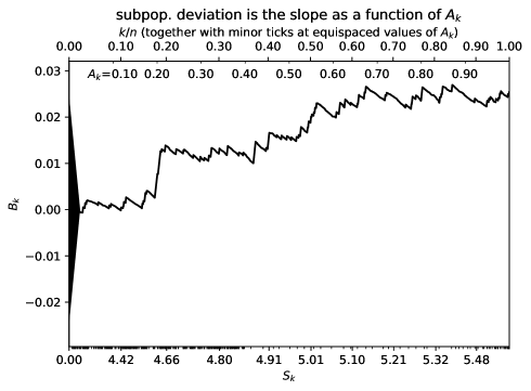
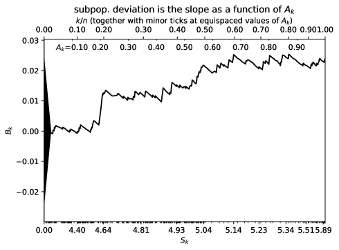
for $\ell=1$, $2$, …, $n$. Figures 6, 7, and 8 of Subsection 3.2 below plot $B_{1}$, $B_{2}$, …, $B_{n}$ versus $A_{1}$, $A_{2}$, …, $A_{n}$ for some numerical examples. A simple calculation of Tygert (2021a) shows that the expected slope of the line graph of $B_{1}$, $B_{2}$, …, $B_{n}$ versus $A_{1}$, $A_{2}$, …, $A_{n}$ from $A_{k-1}$ to $A_{k}$ is $\operatorname{\mathop{}\mathbb{E}}[R_{k}]-r(S_{k})$; that is, the expected slope is simply the deviation of the expected response from the full population’s, in a graph for which $A_{1}$, $A_{2}$, …, $A_{n}$ are the abscissae (the horizontal coordinates) and $B_{1}$, $B_{2}$, …, $B_{n}$ are the ordinates (the vertical coordinates). Thus, steep slope over a long range indicates significant weighted average deviation over that range. Indeed, the slope of the secant line connecting two points on the graph becomes the weighted average deviation over the long range of scores between those points.

In particular, absence of significant deviation results in a flat graph that is nearly horizontal. Two metrics which measure deviations away from 0 (thus characterizing “goodness-of-fit”) are the maximum absolute value

$$G=\max_{1\leq k\leq n}|B_{k}|$$ (19)

and the range (the maximum value minus the minimum value)

$$H=\max_{0\leq k\leq n}B_{k}-\min_{0\leq k\leq n}B_{k},$$ (20)

where $B_{0}=0$; Remark 1 of Tygert (2021a) justifies including $B_{0}=0$, a justification analogous to why Kuiper (1962) introduced an analogous statistic decades earlier in a related context. The absolute value of the total deviation $\sum_{k\in I}(R_{k}-r(S_{k}))\,W_{k}\Big{/}\sum_{k=1}^{n}W_{k}$ over any interval $I$ of indices is less than or equal to $H$; indeed,

$$H=\max_{I}\left|\frac{\sum_{k\in I}(R_{k}-r(S_{k}))\,W_{k}}{\sum_{k=1}^{n}W_{k}}\right|,$$ (21)

where the maximum is over every interval $I$ of indices. The statistic $G$ is due to Kolmogorov (1933) and Smirnov (1939); $H$ is due to Kuiper (1962).

Under the null hypothesis that the response at every score $s$ is an independent Bernoulli variate taking the value $1$ with probability $r(s)$ and the value $0$ with probability $1-r(s)$, calibrating attained significance levels (P-values) for these statistics involves normalization by

$$\sigma=\frac{\sqrt{\sum_{k=1}^{n}r(S_{k})\cdot(1-r(S_{k}))\cdot(W_{k})^{2}}}{\sum_{k=1}^{n}W_{k}};$$ (22)

of course, such a null hypothesis can be appropriate only when each $R_{k}$ is either 0 or 1, for each $k=1$, $2$, …, $n$. More generally, under a null hypothesis for which the response at score $s$ is expected to have a variance $v(s)$ centered around $r(s)$, the normalization would be by the quantity

$$\sigma=\frac{\sqrt{\sum_{k=1}^{n}v(S_{k})\cdot(W_{k})^{2}}}{\sum_{k=1}^{n}W_{k}};$$ (23)

needless to say, $v(s)=r(s)\cdot(1-r(s))$ for a Bernoulli variate taking the value $1$ with probability $r(s)$ and the value $0$ with probability $1-r(s)$, consistent with (22). “Normalization” means considering the ratios $G/\sigma$ and $H/\sigma$ rather than the unnormalized $G$ and $H$ from (19) and (20).

In many cases in practice, such a large sample of the full population is available that $r$ and $v$ can be estimated to high accuracy from the data; Tygert (2021a) elaborates methods for such estimation. The estimates of $v$ used in Section 3 of the present paper adjust for bias via dividing by 1 minus the ratio of the sum of the squares of the weights to the square of the sum of the weights. When all weights are equal, this adjustment simply multiplies by $m/(m-1)$, where $m$ is the number of weights, so that the estimate of the variance involves dividing by $m-1$ (rather than by $m$) in the calculation of the empirical variance. While the present paper makes no claim whatsoever as to the proper resolution of the historic debate about whether estimates of the variance should involve dividing by $m$ or by $m-1$, the estimates (when used in the context of the cumulative statistics) did improve very slightly when adjusting for bias in the estimates.

2.3 Calibration of P-values for the Kolmogorov-Smirnov statistic and the Kuiper statistic

This subsection derives Corollary 9, providing a method for the calculation of attained significance levels (P-values) for the Kolmogorov-Smirnov and Kuiper metrics introduced in the previous subsection.

Propositions 1–4 of Diebolt (1995) prove the following theorem. Technically, Diebolt (1995) provides much stronger and more general results, characterizing not only convergence but also the convergence rates. See also closely related results of Stute (1997). Earlier results of Delgado (1993) motivated the work of Diebolt (1995) and Stute (1997) (among others), and are also closely related to the metrics of Tygert (2021b). The proofs of Delgado (1993) are in some ways simpler and easier to grasp, despite being restricted to a somewhat more special case, and are a superb starting point in addition to being of substantial independent importance, both practically and theoretically.

Theorem 7.

Assume the null hypothesis that the subpopulation has no expected deviation from the full population (that is, $\operatorname{\mathop{}\mathbb{E}}[R_{k}]=r(S_{k})$ for $k=1$, $2$, …, $n$) and that the third moment obeys $\operatorname{\mathop{}\mathbb{E}}[|R_{k}-r(S_{k})|^{3}]\leq C(v(S_{k}))^{3/2}$ for $k=1$, $2$, …, $n$, where $C$ is a finite positive real number that does not depend on $n$. Suppose that the scores $S_{1}$, $S_{2}$, …, $S_{n}$ are distinct for each $n$ and $\max_{1\leq k\leq n}v(S_{k})\cdot(W_{k})^{2}/\sum_{j=1}^{n}v(S_{j})\cdot(W_{j})^{2}$ converges to 0 in the limit as $n$ becomes large. Then, with $G$ defined in (19) and $\sigma$ defined in (23), the normalized Kolmogorov-Smirnov statistic $G/\sigma$ for measuring deviation of a subpopulation from the full population converges in distribution to the maximum of the absolute value of the standard Brownian motion over the unit interval $[0,1]$. The normalized Kolmogorov-Smirnov statistic $G/\sigma$ for measuring calibration converges in distribution to the maximum of the absolute value of the standard Brownian motion over the unit interval $[0,1]$, too, when taking the expected response at each score to be equal to the score, that is, $r(s)=s$ for every score $s$.

The theorems of Diebolt (1995) similarly yield the analogous theorem for the Kuiper statistic:

Theorem 8.

Assume the null hypothesis that the subpopulation has no expected deviation from the full population (that is, $\operatorname{\mathop{}\mathbb{E}}[R_{k}]=r(S_{k})$ for $k=1$, $2$, …, $n$) and that the third moment obeys $\operatorname{\mathop{}\mathbb{E}}[|R_{k}-r(S_{k})|^{3}]\leq C(v(S_{k}))^{3/2}$ for $k=1$, $2$, …, $n$, where $C$ is a finite positive real number that does not depend on $n$. Suppose that the scores $S_{1}$, $S_{2}$, …, $S_{n}$ are distinct for each $n$ and $\max_{1\leq k\leq n}v(S_{k})\cdot(W_{k})^{2}/\sum_{j=1}^{n}v(S_{j})\cdot(W_{j})^{2}$ converges to 0 in the limit as $n$ becomes large. Then, with $H$ defined in (20) and $\sigma$ defined in (23), the normalized Kuiper statistic $H/\sigma$ for measuring deviation of a subpopulation from the full population converges in distribution to the range of the standard Brownian motion over the unit interval $[0,1]$. (The range is the maximum minus the minimum.) The normalized Kuiper statistic $H/\sigma$ for measuring calibration converges in distribution to the range of the standard Brownian motion over the unit interval $[0,1]$, too, when taking the expected response at each score to be equal to the score, that is, $r(s)=s$ for every score $s$.

Putting everything together yields the following.

Corollary 9.

Taking 1 and subtracting the function $D$ from (14) applied to the normalized Kolmogorov-Smirnov statistic $G/\sigma$ yields estimates which converge in distribution to the asymptotic P-value as $n$ becomes large (due to Theorems 5 and 7) — this is $1-D(G/\sigma)$. Evaluating 1 minus the function $F$ from (1) applied to the normalized Kuiper statistic $H/\sigma$ yields estimates which converge in distribution to the asymptotic P-value as $n$ becomes large (due to Theorems 3 and 8) — this is $1-F(H/\sigma)$. The Kolmogorov-Smirnov metric $G$ is defined in (19), the Kuiper metric $H$ is defined in (20), and the normalizing factor $\sigma$ is defined in (23), with (23) reducing to (22) when the responses are Bernoulli variates.

2.4 Ties in ranking scores can be treated as weighted samples

Subsection 2.2 above suggests making minute random perturbations to the scores in order to ensure that the scores are distinct from each other. The present subsection proposes an alternative to breaking ties at random. The present subsection constructs from the original data a weighted data set that modifies the scores, weights, and responses such that the new scores are unique and (together with the new weights and responses) yield cumulative statistics that are consistent with those computed with the original data. This reduces the problem of analyzing data with scores that may not be unique to the problem of analyzing a weighted data set with scores that are unique by construction. The earlier subsections have already detailed how to process weighted samples whose scores are all distinct from each other.

The formulation of the present subsection is merely an alternative, not necessarily superior. The alternative formulation requires no randomization of the data analysis, unlike the earlier analyses. The graphs of the earlier analyses directly displayed all members of the original data set, omitting no one. In contrast, for each score that multiple individuals share, the graphs for the formulation of the present subsection display only the average of those multiple individuals’ responses. Nevertheless, the corresponding scalar summary statistics have the same interpretations and asymptotic calibrations of P-values. Thus, the earlier and new formulations have advantages and disadvantages relative to each other (though none of the disadvantages is substantial, admittedly). Both are good options to have available.

The previous subsections directly analyzed only data sets in which the scores are all unique:

$$S_{1}<S_{2}<\dots<S_{n},$$ (24)

where the inequalities are all strict. The present subsection considers the case in which each score $S_{k}$ may appear multiple times — say $n_{k}$ times — in the data set. With this notation of $n_{k}$ specifying the degeneracy of score $S_{k}$, we define $W_{k}$ to be the sum of all $n_{k}$ of the original weights associated with score $S_{k}$; denoting the original weights by $W_{k}^{(1)}$, $W_{k}^{(2)}$, …, $W_{k}^{(n_{k})}$, we thus define

$$W_{k}=\sum_{j=1}^{n_{k}}W_{k}^{(j)}$$ (25)

for $k=1$, $2$, …, $n$. We define $R_{k}$ to be the weighted average of all $n_{k}$ of the original real-valued responses associated with score $S_{k}$; denoting the original responses by $R_{k}^{(1)}$, $R_{k}^{(2)}$, …, $R_{k}^{(n_{k})}$, we thus define

$$R_{k}=\frac{\sum_{j=1}^{n_{k}}R_{k}^{(j)}\,W_{k}^{(j)}}{\sum_{j=1}^{n_{k}}W_{k}^{(j)}}$$ (26)

for $k=1$, $2$, …, $n$. This yields a data set consisting of the weighted sample $(S_{k},R_{k},W_{k})$ for $k=1$, $2$, …, $n$, where $S_{k}$ is the score, $R_{k}$ is the associated response, and $W_{k}$ is the associated weight. So this new weighted data set contains $n$ members $(S_{k},R_{k},W_{k})$ for $k=1$, $2$, …, $n$, whereas the original data set contains $\sum_{k=1}^{n}n_{k}$ members $(S_{k}^{(j)},R_{k}^{(j)},W_{k}^{(j)})$ for $k=1$, $2$, …, $n$; $j=1$, $2$, …, $n_{k}$. Analyzing the new weighted data set via the cumulative statistics is a good way to analyze the original data set. And, unlike the scores for the original data set, the scores for the new weighted data set are guaranteed to be unique.

We now show that the cumulative statistics for the original and new data sets are consistent with each other.

The cumulative differences for the new data are

$$C_{\ell}=\frac{\sum_{k=1}^{\ell}(R_{k}-r(S_{k}))\,W_{k}}{\sum_{k=1}^{n}W_{k}}$$ (27)

for $\ell=1$, $2$, …, $n$, where $r$ is the regression function we seek to test; when testing calibration, the regression function $r$ is simply the identity function $r(s)=s$ for every real number $s$. When comparing a subpopulation to the full population, $r(S_{k})$ would be the (weighted) average of responses from the full population at scores that are closer to $S_{k}$ than to any other of the scores $S_{1}$, $S_{2}$, …, $S_{n}$. We set $C_{0}=0$, too.

Let us denote by $v(R_{k})$ the variance of the response $R_{k}$ corresponding to the score $S_{k}$ under the null hypothesis, where the null hypothesis makes assumptions about the original data directly (so that inferences about $R_{k}$ take into account the fact that $R_{k}$ is a weighted average of other random variables, instead of considering $R_{k}$ to be a single response variable). For example, under the null hypothesis of perfect calibration with each response drawn independently from a Bernoulli distribution,

$$v(R_{k})=S_{k}\,(1-S_{k})\,\frac{\sum_{j=1}^{n_{k}}\left(W_{k}^{(j)}\right)^{2}}{\left(\sum_{j=1}^{n_{k}}W_{k}^{(j)}\right)^{2}},$$ (28)

since $S_{k}\,(1-S_{k})$ is the variance of the Bernoulli distribution whose expected value is $r(S_{k})=S_{k}$. Calibration need not be the only hypothesis of interest to test. Under the null hypothesis that a subpopulation being assessed does not deviate from the function $r$ for the full population, an estimate of $v(R_{k})$ can be the (weighted) average of variances of responses from the full population at scores that are closer to $S_{k}$ than to any other of the scores $S_{1}$, $S_{2}$, …, $S_{n}$ (assuming as always that the responses are all independent), multiplied by the same factor from (28), namely

$$\frac{\sum_{j=1}^{n_{k}}\left(W_{k}^{(j)}\right)^{2}}{\left(\sum_{j=1}^{n_{k}}W_{k}^{(j)}\right)^{2}};$$ (29)

indeed, the independence of all the responses yields that $v(R_{k})$ is equal to the quantity in (29) times the variance of $R_{k}^{(j)}$, for every $j=1$, $2$, …, $n_{k}$; $k=1$, $2$, …, $n$. Tygert (2021a) gives the details. Since we assumed that the responses are independent, the variance of $C_{\ell}$ from (27) under the null hypothesis is

$$(\sigma_{\ell})^{2}=\frac{\sum_{k=1}^{\ell}v(R_{k})\cdot(W_{k})^{2}}{(\sum_{k=1}^{n}W_{k})^{2}}$$ (30)

for $\ell=1$, $2$, …, $n$.

We also consider similar cumulative differences for the original data set in which the scores are perturbed infinitesimally at random (so that the scores become unique):

$$B_{\ell}=\frac{\sum_{k=1}^{\ell}\sum_{j=1}^{n_{k}}\left(R_{k}^{(j)}-r(S_{k})\right)\,W_{k}^{(j)}}{\sum_{k=1}^{n}\sum_{j=1}^{n_{k}}W_{k}^{(j)}}=\frac{\sum_{k=1}^{\ell}(R_{k}-r(S_{k}))\sum_{j=1}^{n_{k}}W_{k}^{(j)}}{\sum_{k=1}^{n}\sum_{j=1}^{n_{k}}W_{k}^{(j)}}$$ (31)

for $\ell=1$, $2$, …, $n$, where the ordering of $R_{k}^{(1)}$, $R_{k}^{(2)}$, …, $R_{k}^{(n_{k})}$ (and the corresponding weights) is randomized for each $k=1$, $2$, …, $n$. We set $B_{0}=0$, too.

We define abscissae via the aggregations

$$A_{\ell}=\frac{\sum_{k=1}^{\ell}\sum_{j=1}^{n_{k}}W_{k}^{(j)}}{\sum_{k=1}^{n}\sum_{j=1}^{n_{k}}W_{k}^{(j)}}=\frac{\sum_{k=1}^{\ell}W_{k}}{\sum_{k=1}^{n}W_{k}}$$ (32)

for $\ell=1$, $2$, …, $n$, where the latter equality follows from (25). We set $A_{0}=0$, too. Combining (25), (27), and (31) shows that $B_{\ell}=C_{\ell}$ for all $\ell=1$, $2$, …, $n$. Therefore, the piecewise linear graph connecting the points $(A_{\ell},\,B_{\ell}/\sigma_{n})$ for $\ell=0$, $1$, $2$, …, $n$ and the piecewise linear graph connecting the points $(A_{\ell},\,C_{\ell}/\sigma_{n})$ for $\ell=0$, $1$, $2$, …, $n$ are the same. This demonstrates that the cumulative statistics for the original and new data sets are consistent with each other. Indeed, the corresponding graph of cumulative differences for the original data with its scores perturbed very slightly (so that the scores become unique) is the same aside from the other graphs linearly interpolating from each score $S_{k}$ to the next greatest score, $S_{k+1}$, rather than interpolating linearly from each and every perturbed score to the next greatest perturbed score.

Theorems 7 and 8 and their Corollary 9 yield the same consequences for all cumulative statistics considered here, under the condition (expressed in the notation of the present subsection):

$$\frac{\max_{1\leq k\leq n}\left[v(R_{k})\cdot\frac{\left(\sum_{j=1}^{n_{k}}W_{k}^{(j)}\right)^{2}}{\sum_{j=1}^{n_{k}}\left(W_{k}^{(j)}\right)^{2}}\cdot\max_{1\leq j\leq n_{k}}\left(W_{k}^{(j)}\right)^{2}\right]}{\sum_{k=1}^{n}\left[v(R_{k})\cdot\left(\sum_{j=1}^{n_{k}}W_{k}^{(j)}\right)^{2}\right]}$$ (33)

converges to 0 in the limit as $n$ becomes large. The denominator in (33) is simply the numerator in (33) after replacing the maximizations with sums.

To summarize: the cumulative statistics for the original data set can require perturbing the scores slightly in order to break degeneracies, unlike the cumulative statistics for the new weighted data. The randomization does preserve more information about the original data, as the associated graph of cumulative differences displays the response of every single individual from the original data set. The new weighted data set instead avoids any randomization but, for each score that multiple members share, averages together the multiple members’ responses. Thus both the previous approaches and that of the present subsection have pros and cons relative to each other. That said, the approaches are more similar than different; neither has any substantial drawback.

3 Results

The present section illustrates (via examples and plots) the numerical and graphical methods of the preceding section. Subsection 3.1 verifies the methods numerically, double-checking the rigorous proofs given earlier. Subsection 3.2 applies the methods to a popular data set from the U.S. Census Bureau.

3.1 Numerical validation

This subsection presents numerical verifications of the methods of the preceding section. The numerical validation is purely supplemental, as the proofs given earlier are complete on their own. The numerical results are nice and concrete, possibly easier to digest than the detailed proofs.

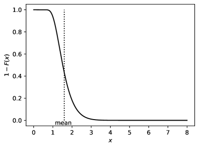
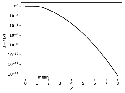
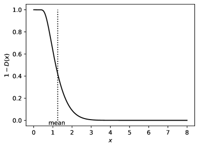
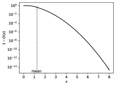
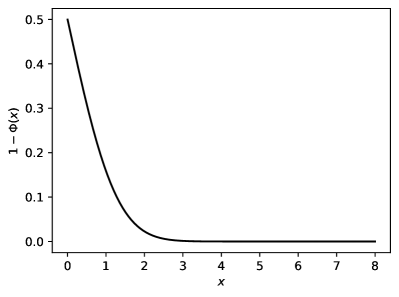
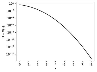
Figures 1 and 2 plot $1-F(x)$ versus $x$ and $1-D(x)$ versus $x$, respectively, where $F$ is defined in (1) and $D$ is defined in (14). The calculation for $F$ truncates the series in (1) after $n$ terms, where $n=n(x)$ is the least integer such that (9) guarantees full double-precision accuracy (with $\varepsilon\approx$ 2.2E–16). Similarly, the calculation for $D$ truncates the series in (14) after $n$ terms, where $n=n(x)$ is the least integer such that (16) guarantees full double-precision accuracy (again with $\varepsilon\approx$ 2.2E–16). To give an indication of how another sub-Gaussian distribution decays, Figure 3 plots $1-\Phi(x)$ versus $x$, where $\Phi$ is the cumulative distribution function for the standard normal distribution.

Formula 1.4 of Feller (1951) and Formula 46 of Masoliver (2014) give the means of the distributions associated with the cumulative distribution functions $F$ and $D$ defined in (1) and (14), as $2\sqrt{2/\pi}\approx 1.5958$ and $\sqrt{\pi/2}\approx 1.2533$, respectively. The horizontal positions of the vertical dotted lines labeled “mean” in Figures 1 and 2 are at these mean values. A unit test of the implementations of the cumulative distribution functions is to numerically evaluate the means. Using a Gauss-Chebyshev quadrature of order 100,000 to integrate $1-F(x)$ and $1-D(x)$ from $x=$ 1E–8 to $x=8$ yields the correct means to better than 8-digit relative accuracy in the implemented codes, thus passing this unit test.

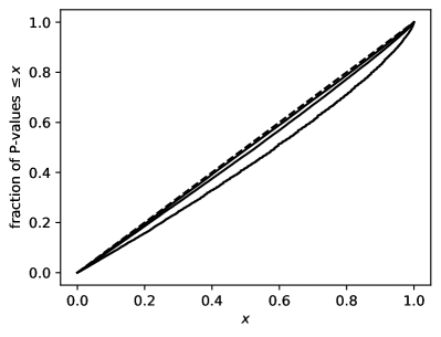
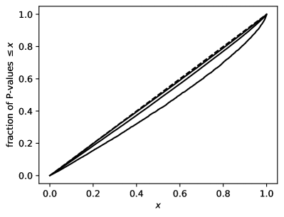
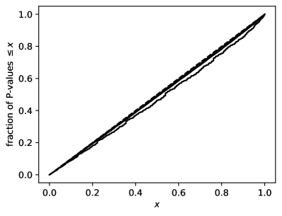
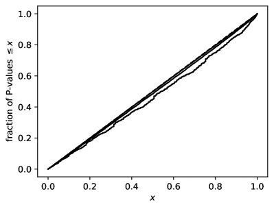
Figures 4 and 5 plot the calibration curves for the Kuiper and Kolmogorov-Smirnov statistics, respectively. The calibration curves are the empirical cumulative distribution functions of the asymptotic P-values for calibration calculated for 100,000 data sets generated by drawing independent Bernoulli responses at the scores, with the probability of success in the Bernoulli distribution being exactly equal to the score (so that the data is perfectly calibrated, by construction). Perfectly calibrated P-values would follow the uniform distribution over the unit interval $[0,1]$ under the null hypothesis, and so ideally the plotted empirical cumulative distribution functions should approach the cumulative distribution function for the uniform distribution as the sample size increases. The cumulative distribution function for the uniform distribution over the unit interval $[0,1]$ is the line connecting the origin $(0,0)$ to the point $(1,1)$; each plot displays a dashed line to indicate the ideal calibration curve. The other curves are the empirical cumulative distribution functions of the P-values for data sets with sample sizes $n=$ 100, 1,000, 10,000; as expected, the curve closest to the diagonal dashed line in each plot is that for $n=$ 10,000, the next closest is for $n=$ 1,000, and the farthest is for $n=$ 100. The weights in these synthetically generated data sets are uniform (all equal), just for simplicity.

Figures 4 and 5 illustrate Corollary 9, with convergence to the ideal calibration that Delgado (1993), Diebolt (1995), and Stute (1997) prove as the scores become dense in the unit interval $[0,1]$ (the scores are quite dense already with $n=$ 10,000, for example). Notice that the empirical curves all lie entirely below the diagonal dashed line, in accordance with the calculated finite-sample P-values being conservatively calibrated (the P-values are not smaller on average than expected).

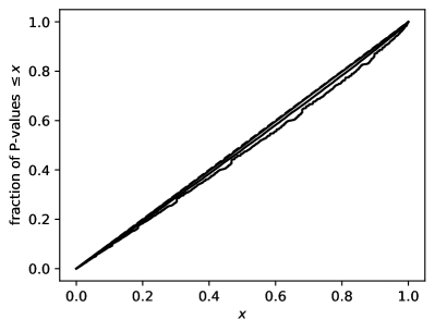
The ends of the captions of Figures 6, 7, and 8 from the following subsection report P-values evaluated using Corollary 9. Attained significance levels (P-values) for all methods of Tygert (2021a) can also be calibrated and calculated directly using Corollary 9, under the assumption that, for each of the scores from the subpopulation, the full population contains many members whose scores are closer to the score from the subpopulation than to other scores from the subpopulation; if this assumption is invalid, then the statistics fed into the cumulative distribution functions require adjustment to account for the additional stochasticity, as described by Tygert (2021a) and Tygert (2021b).

3.2 Data analysis

This subsection illustrates the methods of the preceding section by applying the methods to the microdata of the U.S. Census Bureau’s 2019 American Community Survey. We discard every member of the data set for which the weight (“WGTP” in the microdata) for the weighted sampling is zero, as well as every member for which household personal income (“HINCP”) is zero and every member for which the adjustment factor to income (“ADJINC”) is reported as missing. The scores are the logarithm to base 10 of the adjusted household personal income (the adjusted income is “HINCP” times “ADJINC,” divided by one million; the one million accounts for the omission of any decimal point in “ADJINC” — the microdata is integer-valued). The responses are the variables from the data set specified in the captions to the figures for this subsection, namely Figures 6–8 (different figures analyze different response variables). The full population in the survey consists of 134,094 households, a weighted sample of California. The subpopulation being compared to the full population consists of the households in the county specified in the caption to the corresponding figure.

4 Discussion and conclusion

As shown above, the combination of Feller (1951), Darling and Siegert (1953), Delgado (1993), Diebolt (1995), Stute (1997), and others trivially yields computationally efficient and convenient calibration of P-values for the metrics of Tygert (2021a), metrics very similar to those of Kolmogorov (1933) and Smirnov (1939) and of Kuiper (1962) (whose work directly stimulated all the others’, including that of the author of the present paper). The results of Delgado (1993), Diebolt (1995), and Stute (1997) reduce the problem of calibration to the calculation of the distributions of the range and of the maximum absolute value of the standard Brownian motion over the unit interval $[0,1]$; the results of Feller (1951) and Darling and Siegert (1953) completely characterize those distributions. Simple, straightforward manipulation of the resulting formulae then yields the cumulative distribution functions required for calibrating P-values, as detailed in Section 2 above. Section 2 also presents two different approaches for processing data sets in which the scores are not all distinct from each other. In all cases, implementation is easy; Section 3 validates the numerical methods and implementation via plots of the cumulative distribution functions of the metrics and of the associated P-values, as well as via checks against analytic, closed-form expressions, illustrating use of the codes both on their own and as applied to both real and synthetic data sets. The software is ready for widespread use under its permissive MIT copyright license.

Figure 1: Both plots graph $1-F(x)$ versus $x$, where $F$ is defined in (1) and is central to Corollary 9. The plot on the right uses a logarithmic scale for the vertical axis, unlike the plot on the left. The vertical dotted line indicates the value of $x$ corresponding to the mean of the distribution for which $F$ is the cumulative distribution function.

Figure 2: Both plots graph $1-D(x)$ versus $x$, where $D$ is defined in (14) and is central to Corollary 9. The plot on the right uses a logarithmic scale for the vertical axis, unlike the plot on the left. The vertical dotted line indicates the value of $x$ corresponding to the mean of the distribution for which $D$ is the cumulative distribution function.

Figure 3: Both plots graph $1-\Phi(x)$ versus $x$, where $\Phi$ is the cumulative distribution function for the standard normal distribution; $\Phi(x)=\int_{-\infty}^{x}\exp(-y^{2}/2)\,dy\,/\,\sqrt{2\pi}$. The plot on the right uses a logarithmic scale for the vertical axis, unlike the plot on the left.

(a)

(b)    (c)

Figure 4: Calibration curves (empirical cumulative distribution functions under the null hypothesis of perfectly calibrated data) of the Kuiper P-value for calibration for sample sizes $n=$ 100, 1,000, 10,000; in each plot, the dashed line connects the origin $(0,0)$ to the point $(1,1)$ and illustrates perfect calibration, while the curve for $n=$ 10,000 is closest to perfect, $n=$ 1,000 is next closest, and $n=$ 100 is the farthest. Subfigure (a) uses scores equispaced on the unit interval $[0,1]$, (b) squares each of the initially equispaced scores, and (c) takes the square root of each of the initially equispaced scores. The score $s$ is the predicted probability, with the expected response $r(s)=s$ to assess calibration. Each empirical cumulative distribution function plotted arises from 100,000 data sets generated independently while assuming the null hypothesis.

(a)

(b)    (c)

Figure 5: Calibration curves (empirical cumulative distribution functions under the null hypothesis of perfectly calibrated data) of the Kolmogorov-Smirnov P-value for calibration for sample sizes $n=$ 100, 1,000, 10,000; in each plot, the dashed line connects the origin $(0,0)$ to the point $(1,1)$ and illustrates perfect calibration, while the curve for $n=$ 10,000 is closest to perfect, $n=$ 1,000 is next closest, and $n=$ 100 is the farthest. Subfigure (a) uses scores equispaced on the unit interval $[0,1]$, (b) squares each of the initially equispaced scores, and (c) takes the square root of each of the initially equispaced scores. The score $s$ is the predicted probability, with the expected response $r(s)=s$ to assess calibration. Each empirical cumulative distribution function plotted arises from 100,000 data sets generated independently while assuming the null hypothesis.

($n=$ 35,364)

($n=$ 5,587)

Figure 6: Difference in the number of people in a household between the county of Los Angeles and the entire state of California (the county is the subpopulation, while the state is the full population). The scores indicated along the lower horizontal axis are $\log_{10}$ of the adjusted household income, randomly perturbed in the upper plot by about one part in a hundred million to ensure their uniqueness. There are 35,364 households representing Los Angeles. When the scores are perturbed at random ($n=$ 35,364), Kuiper’s statistic $H=0.06674$, while $H/\sigma=7.521$; Kolmogorov’s and Smirnov’s $G=0.06495$, while $G/\sigma=7.319$. When the responses are averaged for the same score as in Subsection 2.4 and displayed in the lower plot ($n=$ 5,587), Kuiper’s statistic $H=0.07126$, while $H/\sigma_{n}=7.213$; Kolmogorov’s and Smirnov’s $G=0.06736$, while $G/\sigma_{n}=6.818$. The P-values for both statistics are 0 to the precision of computations. These P-values reflect the observed difference of many standard deviations beyond the expected means. Deviation of the subpopulation’s response (the number of people) from the full population’s is the slope as displayed.

($n=$ 1,624)

($n=$ 892)

Figure 7: Difference in the number of children related to the head of household between the county of Stanislaus and the entire state of California (the county is the subpopulation, while the state is the full population). The scores indicated along the lower horizontal axis are $\log_{10}$ of the adjusted household income, randomly perturbed in the upper plot by about one part in a hundred million to guarantee their uniqueness. There are 1,624 households representing Stanislaus. When the scores are perturbed at random ($n=$ 1,624), Kuiper’s statistic $H=0.1489$, while $H/\sigma=4.373$; Kolmogorov’s and Smirnov’s $G=0.1467$, while $G/\sigma=4.307$. When the responses are averaged for the same score ($n=$ 892), Kuiper’s statistic $H=0.1575$, while $H/\sigma_{n}=4.710$; Kolmogorov’s and Smirnov’s $G=0.1547$, while $G/\sigma_{n}=4.624$. The estimates of P-values for Kuiper’s statistic are 4.902E–5 and 0.991E–5; the estimates of P-values for Kolmogorov’s and Smirnov’s are 3.310E–5 and 0.753E–5. These P-values reflect the observed difference of several standard deviations beyond the expected means. Deviation of the subpopulation from the full population is the slope.

($n=$ 679)

($n=$ 506)

Figure 8: Difference in whether a household has internet access via satellite between the county of Napa and the entire state of California (the county is the subpopulation, while the state is the full population). The scores indicated along the lower horizontal axis are $\log_{10}$ of the adjusted household income, randomly perturbed by about one part in a hundred million to ensure their uniqueness. There are 679 households representing Napa. When the scores are perturbed at random ($n=$ 679), Kuiper’s statistic $H=0.02761$, while $H/\sigma=2.259$; Kolmogorov’s and Smirnov’s $G=0.02695$, while $G/\sigma=2.205$. When the responses are averaged for the same score ($n=$ 506), Kuiper’s statistic $H=0.02619$, while $H/\sigma_{n}=2.110$; Kolmogorov’s and Smirnov’s $G=0.02537$, while $G/\sigma_{n}=2.043$. The estimates of P-values for Kuiper’s statistic are 0.0955 and 0.1392; the estimates of P-values for Kolmogorov’s and Smirnov’s are 0.0549 and 0.0821. The P-values reflect the observed difference of not even a couple standard deviations beyond the expected means. Deviation of the subpop.’s response (1 if satellite; 0 otherwise) from the full population’s is the slope.

References

- Ciesielski and Taylor (1962) Ciesielski, Z. and Taylor, S. J. (1962), “First passage times and sojourn times for Brownian motion in space and the exact Hausdorff measure of the sample path,” Trans. Amer. Math. Soc., 103, 434–450.
- Darling and Siegert (1953) Darling, D. A. and Siegert, A. J. F. (1953), “The first passage problem for a continuous Markov process,” Ann. Math. Statist., 24, 624–639.
- Delgado (1993) Delgado, M. A. (1993), “Testing the equality of nonparametric regression curves,” Statist. Probab. Lett., 17, 199–204.
- Diebolt (1995) Diebolt, J. (1995), “A nonparametric test for the regression function: asymptotic theory,” J. Statist. Plann. Inference, 44, 1–17.
- Feller (1951) Feller, W. (1951), “The asymptotic distribution of the range of sums of independent random variables,” Ann. Math. Statist., 22, 427–432.
- Kolmogorov (1933) Kolmogorov, A. N. (1933), “Sulla determinazione empirica di una legge di distribuzione (On the empirical determination of a distribution function),” Giorn. Ist. Ital. Attuar., 4, 83–91.
- Kuiper (1962) Kuiper, N. H. (1962), “Tests concerning random points on a circle,” Proc. Koninklijke Nederlandse Akademie van Wetenschappen Series A, 63, 38–47.
- Masoliver (2014) Masoliver, J. (2014), “Extreme values and the level-crossing problem: an application to the Feller process,” Phys. Rev. E, 89. No. 042106.
- Smirnov (1939) Smirnov, N. (1939), “On the estimation of the discrepancy between empirical curves of distribution for two independent samples,” Bulletin Mathématique de l’Université de Moscou, 2, 3–11.
- Stute (1997) Stute, W. (1997), “Nonparametric model checks for regression,” Ann. Statist., 25, 613–641.
- Tygert (2021a) Tygert, M. (2021a), “Cumulative deviation of a subpopulation from the full population,” J. Big Data, 8, 1–60, URL https://arxiv.org/abs/2008.01779.
- Tygert (2021b) — (2021b), “A graphical method of cumulative differences between two subpopulations,” J. Big Data, 8, 1–29, URL https://arxiv.org/abs/2108.02666.