Understanding AdamW through Proximal Methods and Scale-Freeness

Abstract

Adam has been widely adopted for training deep neural networks due to less hyperparameter tuning and remarkable performance. To improve generalization, Adam is typically used in tandem with a squared $\ell_{2}$ regularizer (referred to as Adam-$\ell_{2}$). However, even better performance can be obtained with AdamW, which decouples the gradient of the regularizer from the update rule of Adam-$\ell_{2}$. Yet, we are still lacking a complete explanation of the advantages of AdamW. In this paper, we tackle this question from both an optimization and an empirical point of view. First, we show how to re-interpret AdamW as an approximation of a proximal gradient method, which takes advantage of the closed-form proximal mapping of the regularizer instead of only utilizing its gradient information as in Adam-$\ell_{2}$. Next, we consider the property of “scale-freeness” enjoyed by AdamW and by its proximal counterpart: their updates are invariant to component-wise rescaling of the gradients. We provide empirical evidence across a wide range of deep learning experiments showing a correlation between the problems in which AdamW exhibits an advantage over Adam-$\ell_{2}$ and the degree to which we expect the gradients of the network to exhibit multiple scales, thus motivating the hypothesis that the advantage of AdamW could be due to the scale-free updates.

1 Introduction

Recent years have seen a surge of interest in applying deep neural networks (LeCun et al., 2015) to a myriad of areas. While Stochastic Gradient Descent (SGD) (Robbins and Monro, 1951) remains the dominant method for optimizing such models, its performance depends crucially on the step size hyperparameter. To alleviate this problem, there has been a fruitful amount of research on adaptive gradient methods (e.g. Duchi et al., 2010a; McMahan and Streeter, 2010; Tieleman and Hinton, 2012; Zeiler, 2012; Luo et al., 2018; Zhou et al., 2018). These methods provide mechanisms to automatically set stepsizes and have been shown to greatly reduce the tuning effort while maintaining good performance. Among those adaptive algorithms, one of the most widely used is Adam (Kingma and Ba, 2015) which achieves good results across a variety of problems even by simply adopting the default hyperparameter setting.

In practice, to improve the generalization ability, Adam is typically combined with a squared $\ell_{2}$ regularization, which we will call Adam-$\ell_{2}$ hereafter. Yet, as pointed out by Loshchilov and Hutter (2019), the gradient of the regularizer does not interact properly with the Adam update rule. To address this, they provide a method called AdamW that decouples the gradient of the $\ell_{2}$ regularization from the update of Adam. The two algorithms are shown in Algorithm 1. Although AdamW is very popular (Kuen et al., 2019; Lifchitz et al., 2019; Carion et al., 2020) and it frequently outperforms Adam-$\ell_{2}$, it is currently unclear why it works so well. Recently, however, Bjorck et al. (2020) applied AdamW in Natural Language Processing and Reinforcement Learning problems and found no improvement of performance over sufficiently tuned Adam-$\ell_{2}$.

In this paper, we focus on understanding how the AdamW update differs from Adam-$\ell_{2}$ from an optimization point of view. First, we unveil the surprising connection between AdamW and proximal updates (Parikh and Boyd, 2014). In particular, we show that AdamW is an approximation of the latter and confirm such similarity with an empirical study. Moreover, noticing that AdamW and the proximal update are both scale-free while Adam-$\ell_{2}$ is not, we also derive a theorem showing that scale-free optimizers enjoy an automatic acceleration w.r.t. the condition number on certain cases. This gives AdamW a concrete theoretical advantage in training over Adam-$\ell_{2}$.

Next, we empirically identify the scenario of training very deep neural networks with Batch Normalization switched off as a case in which AdamW substantially outperforms Adam-$\ell_{2}$ in both testing and training. In such settings, we observe that the magnitudes of the coordinates of the updates during training are much more concentrated about a fixed value for AdamW than for Adam-$\ell_{2}$, which is an expected property of scale-free algorithms. Further, as depth increases, we expect a greater diversity of gradient scalings, a scenario that should favor scale-free updates. Our experiments support this hypothesis: deeper networks have more dramatic differences between the distributions of update scales between Adam-$\ell_{2}$ and AdamW and exhibit larger accuracy advantages for AdamW.

To summarize, the contributions of this paper are:

1. We show that AdamW can be seen as an approximation of a proximal update, which utilizes the entire regularizer rather than only its gradient.

2. We point out the scale-freeness property enjoyed by AdamW and show the advantage of such a property on a class of functions.

3. We find a scenario where AdamW is significantly better than Adam-$\ell_{2}$ in both training and testing performance and report an empirical observation of the correlation between such advantage and the scale-freeness property of AdamW.

The rest of this paper is organized as follows: In Section 2 we discuss the relevant literature. The connection between AdamW and the proximal updates as well as its scale-freeness are explained in Section 3. We then report the empirical observations in Section 4. Finally, we conclude with a discussion of the results, some limitations of this work, and future directions.

2 Related Work

Weight decay By biasing the optimization towards solutions with small norms, weight decay has long been a standard technique to improve the generalization ability in machine learning (Krogh and Hertz, 1992; Bos and Chug, 1996) and is still widely employed in training modern deep neural networks (Devlin et al., 2019; Tan and Le, 2019). Note that here we do not attempt to explain the generalization ability of weight decay or AdamW. Rather, we assume that the regularization and the topology of the network guarantee good generalization performance and study training algorithms from an optimization point of view. In this view, we are not aware of other work on the influence of regularization on the optimization process.

Proximal updates The use of proximal updates in the batch optimization literature dates back at least to 1965 (Moreau, 1965; Martinet, 1970; Rockafellar, 1976; Parikh and Boyd, 2014) and they are used more recently even in the stochastic setting (Toulis and Airoldi, 2017; Asi and Duchi, 2019). We are not aware of any previous paper pointing out the connection between AdamW and proximal updates.

Scale-free algorithms The scale-free property was first proposed in the online learning field (Cesa-Bianchi et al., 2007; Orabona and Pál, 2018). There, they do not need to know a priori the Lipschitz constant of the functions, while obtaining optimal convergence rates. To the best of our knowledge, the connection between scale-freeness and the condition number we explain in Section 3 is novel, as is the empirical correlation between scale-freeness and good performance.

Removing Batch Normalization (BN) The setting of removing BN is not our invention: indeed, there is already active research in this (De and Smith, 2020; Zhang et al., 2019). The reason is that BN has many disadvantages (Brock et al., 2021) including added memory overhead (Bulò et al., 2018) and training time (Gitman and Ginsburg, 2017), and a discrepancy between training and inferencing (Singh and Shrivastava, 2019). BN has also been found to be unsuitable for many cases including sequential modeling tasks (Ba et al., 2016) and contrastive learning algorithms (Chen et al., 2020). Also, there are SOTA architectures that do not use BN including the Vision transformer (Dosovitskiy et al., 2021) and the BERT model (Devlin et al., 2019).

3 Theoretical Insights on Merits of AdamW

Algorithm 1 Adam with $\ell_{2}$ regularization (Adam-$\ell_{2}$) and AdamW Loshchilov and Hutter (2017).
All operations on vectors are element-wise.

1:  Given $\alpha$, $\beta_{1}$, $\beta_{2}$, $\epsilon$, $\lambda\in\mathbb{R}$, lr schedule $\{\eta_{t}\}_{t\geq 0}$.

2:  Initialize: $\boldsymbol{x}_{0}\in\mathbb{R}^{d}$, $\boldsymbol{m}_{0}\leftarrow 0$, $\boldsymbol{v}_{0}\leftarrow 0$

3:  for $t=1,2,\ldots,T$ do

4:     Compute the stochastic gradient $\nabla f_{t}(\boldsymbol{x}_{t-1})$

5:     $\boldsymbol{g}_{t}\leftarrow\nabla f_{t}(\boldsymbol{x}_{t-1})$$+\lambda\boldsymbol{x}_{t-1}$

6:     $\boldsymbol{m}_{t}\leftarrow\beta_{1}\boldsymbol{m}_{t-1}+(1-\beta_{1})\boldsymbol{g}_{t}$,  $\boldsymbol{v}_{t}\leftarrow\beta_{2}\boldsymbol{v}_{t-1}+(1-\beta_{2})\boldsymbol{g}_{t}^{2}$

7:     $\hat{\boldsymbol{m}}_{t}\leftarrow\boldsymbol{m}_{t}/(1-\beta_{1}^{t})$,  $\hat{\boldsymbol{v}}_{t}\leftarrow\boldsymbol{v}_{t}/(1-\beta_{2}^{t})$

8:     $\boldsymbol{x}_{t}\leftarrow\boldsymbol{x}_{t-1}$ $-\eta_{t}\lambda\boldsymbol{x}_{t-1}$ $-\eta_{t}\alpha\hat{\boldsymbol{m}}_{t}/(\sqrt{\hat{\boldsymbol{v}}_{t}}+\epsilon)$

9:  end for

AdamW and Proximal Updates Here, we show that AdamW approximates a proximal update.

Consider that we want to minimize the objective function

$$F(\boldsymbol{x})=\tfrac{\lambda}{2}\|\boldsymbol{x}\|_{2}^{2}+f(\boldsymbol{x}),$$ (1)

where $\lambda>0$ and $f(\boldsymbol{x}):\mathbb{R}^{d}\rightarrow\mathbb{R}$ is a function bounded from below. We could use a stochastic optimization algorithm that updates in the following fashion

$$\boldsymbol{x}_{t}=\boldsymbol{x}_{t-1}-M_{t}\boldsymbol{p}_{t},$$ (2)

where $M_{t}$ is a generic matrix containing the learning rates and $\boldsymbol{p}_{t}$ denotes the update direction. Specifically, we consider $M_{t}=\eta_{t}I_{d}$ where $\eta_{t}$ is a learning rate schedule, e.g., the constant one or the cosine annealing (Loshchilov and Hutter, 2017). This update covers many cases:

1. $\boldsymbol{p}_{t}=\alpha\boldsymbol{g}_{t}$ gives us the vanilla SGD;

2. $\boldsymbol{p}_{t}=\alpha\boldsymbol{g}_{t}/(\sqrt{\sum^{t}_{i=1}\boldsymbol{g}_{i}^{2}+\epsilon})$ gives the AdaGrad algorithm (Duchi et al., 2011);

3. $\boldsymbol{p}_{t}=\alpha\hat{\boldsymbol{m}}_{t}/(\sqrt{\hat{\boldsymbol{v}}_{t}}+\epsilon)$ recovers Adam, Algorithm 1,

where $\alpha$ denotes the initial learning rate. Note that in the above we use $\boldsymbol{g}_{t}$ to denote the stochastic gradient of the entire objective function: $\boldsymbol{g}_{t}=\nabla f_{t}(\boldsymbol{x}_{t-1})+\lambda\boldsymbol{x}_{t-1}$ ($\lambda=0$ if the regularizer is not present), with $\hat{\boldsymbol{m}}_{t}$ and $\hat{\boldsymbol{v}}_{t}$ both updated using $\boldsymbol{g}_{t}$.

This update rule (2) is given by the following online mirror descent update (Nemirovsky and Yudin, 1983; Warmuth and Jagota, 1997; Beck and Teboulle, 2003):

$$\boldsymbol{x}_{t}=\mathop{\mathrm{argmin}}_{\boldsymbol{x}\in\mathbb{R}^{d}} \tfrac{\lambda}{2}\|\boldsymbol{x}_{t-1}\|^{2}_{2}+f(\boldsymbol{x}_{t-1})+\boldsymbol{p}_{t}^{\top}(\boldsymbol{x}-\boldsymbol{x}_{t-1})+\tfrac{1}{2}(\boldsymbol{x}-\boldsymbol{x}_{t-1})^{\top}M_{t}^{-1}(\boldsymbol{x}-\boldsymbol{x}_{t-1})~{}.$$ (3)

This approximates minimizing a first-order Taylor approximation of $F$ centered in $\boldsymbol{x}_{t-1}$ plus a term that measures the distance between the $\boldsymbol{x}_{t}$ and $\boldsymbol{x}_{t-1}$ according to the matrix $M^{-1}_{t}$. The approximation becomes exact when $\boldsymbol{p}_{t}=\nabla f(\boldsymbol{x}_{t-1})+\lambda\boldsymbol{x}_{t-1}$.

Yet, this is not the only way to construct first-order updates for the objective (1). An alternative route is to linearize only $f$ and to keep the squared $\ell_{2}$ norm in its functional form:

$$\boldsymbol{x}_{t}=\mathop{\mathrm{argmin}}_{\boldsymbol{x}\in\mathbb{R}^{d}} \tfrac{\lambda}{2}\|\boldsymbol{x}\|^{2}_{2}+f(\boldsymbol{x}_{t-1})+\boldsymbol{p}_{t}^{\top}(\boldsymbol{x}-\boldsymbol{x}_{t-1})+\tfrac{1}{2}(\boldsymbol{x}-\boldsymbol{x}_{t-1})^{\top}M_{t}^{-1}(\boldsymbol{x}-\boldsymbol{x}_{t-1}),$$ (4)

This update rule uses the proximal operator (Moreau, 1965; Parikh and Boyd, 2014) of $\frac{1}{2}\|\cdot\|_{2}^{2}$ w.r.t. the norm $\|\cdot\|_{M_{t}^{-1}}$. It is intuitive why this would be a better update: We directly minimize the squared $\ell_{2}$ norm instead of approximating it.

From the first-order optimality condition, the update is

$$\boldsymbol{x}_{t}=(I_{d}+\lambda M_{t})^{-1}(\boldsymbol{x}_{t-1}-M_{t}\boldsymbol{p}_{t})~{}.$$ (5)

When $\lambda=0$, the update in (2) and this one coincide. Yet, when $\lambda\neq 0$, they are no longer the same.

We now show how the update in (5) generalizes the one in AdamW. The update of AdamW is

$$\boldsymbol{x}_{t}=(1-\lambda\eta_{t})\boldsymbol{x}_{t-1}-\eta_{t}\alpha\hat{\boldsymbol{m}}_{t}/(\sqrt{\hat{\boldsymbol{v}}_{t}}+\epsilon)~{}.$$ (6)

On the other hand, using $M_{t}=\eta_{t}I_{d}$ and $\boldsymbol{p}_{t}=\alpha\hat{\boldsymbol{m}}_{t}/(\sqrt{\hat{\boldsymbol{v}}_{t}}+\epsilon)$ in (5) gives:

$$\boldsymbol{x}_{t}=(1+\lambda\eta_{t})^{-1}(\boldsymbol{x}_{t-1}-\eta_{t}\alpha\hat{\boldsymbol{m}}_{t}/(\sqrt{\hat{\boldsymbol{v}}_{t}}+\epsilon)),$$ (7)

Its first-order Taylor approximation around $\eta_{t}=0$ is

$$\boldsymbol{x}_{t}\approx(1-\lambda\eta_{t})\boldsymbol{x}_{t-1}-\eta_{t}\alpha\hat{\boldsymbol{m}}_{t}/(\sqrt{\hat{\boldsymbol{v}}_{t}}+\epsilon),$$

exactly the AdamW update (6). Hence, AdamW is a first-order approximation of a proximal update.

The careful reader might notice that the approximation from AdamW to the update in (7) becomes less accurate when $\eta_{t}$ becomes too large, and so be concerned whether this approximation is practical at all. Fortunately, in practice, $\eta_{t}$ is never large enough for this to be an issue. The remainder term of this approximation is $O(\lambda\eta_{t}^{2})$ which we should always expect to be small as both $\lambda$ and $\eta_{t}$ are small. So, we can expect AdamW and the update in (7) to perform similarly for learning rate schedules $\eta_{t}$ commonly employed in practice, and we will indeed confirm this empirically in Section 4.3.

Let’s now derive the consequences of this connection with proximal updates. First of all, at least in the convex case, the convergence rate of the proximal updates will depend on $\|\nabla f(\boldsymbol{x}_{t})\|^{2}_{M_{t}}$ rather than on $\|\nabla f(\boldsymbol{x}_{t})+\lambda\boldsymbol{x}_{t}\|^{2}_{M_{t}}$ Duchi et al. (2010b). This could be a significant improvement: the regularized loss function is never Lipschitz, so the regularized gradients $\nabla f(\boldsymbol{x}_{t})+\lambda\boldsymbol{x}_{t}$ could be much larger than $\nabla f(\boldsymbol{x}_{t})$ when $f$ itself is Lipschitz.

More importantly, proximal updates are fundamentally better at keeping the weights small. Let us consider a couple of simple examples to see how this could be. First, suppose the weights are already zero. Then, when taking an update according to (2), we increase the weights to $-M_{t}\boldsymbol{p}_{t}$. In contrast, update (5) clearly leads to a smaller value. This is because it computes an update using the regularizer rather than its gradient. As an even more disturbing, yet actually more realistic example, consider the case that $\boldsymbol{x}_{t-1}$ is non-zero, but $\boldsymbol{g}_{t}=\boldsymbol{0}$. In this case, taking an update using (2) may actually increase the weights by causing $\boldsymbol{x}_{t}$ to overshoot the origin. In contrast, the proximal update will never demonstrate such pathological behavior. Notice that this pathological behavior of (2) can be mitigated by properly tuning the learning rate. However, one of the main attractions of adaptive optimizers is that we should not need to tune the learning rate as much. Thus, the proximal update can be viewed as augmenting the adaptive methods with an even greater degree of learning-rate robustness.

AdamW is Scale-Free We have discussed what advantages the proximal step hidden in AdamW can give but have not yet taken into consideration the specific shape of the update. Here instead we will look closely at the $\boldsymbol{p}_{t}$ used in AdamW to show its scale-freeness. Our main claim is: the lack of scale-freeness seems to harm Adam-$\ell_{2}$’s performance in certain scenarios in deep learning, while AdamW preserves the scale-freeness even with an $\ell_{2}$ regularizer. We will motivate this claim theoretically in this section and empirically in Section 4.

An optimization algorithm is said to be scale-free if its iterates do not change when one multiplies any coordinate of all the gradients of the losses $f_{t}$ by a positive constant (Orabona and Pál, 2018). It turns out that the update (6) of AdamW and the update (7) are both scale-free when $\epsilon=0$. This is evident for AdamW as the scaling factor for any coordinate of the gradient is kept in both $\hat{\boldsymbol{m}_{t}}$ and $\sqrt{\hat{\boldsymbol{v}_{t}}}$ and will be canceled out when dividing them. (In practical applications, though, $\epsilon$ is very small but not zero, so we empirically verify in Section 4.2 that it is small enough to still approximately ensure the scale-free property.) In contrast, for Adam-$\ell_{2}$, the addition of the weight decay vector to the gradient (Line 5 of Algorithm 1) destroys this property.

We want to emphasize the comparison between Adam-$\ell_{2}$ and AdamW: once Adam-$\ell_{2}$ adopts a non-zero $\lambda$, it loses the scale-freeness property; in contrast, AdamW enjoys this property for arbitrary $\lambda$. The same applies to any AdaGrad-type and Adam-type algorithm that incorporates the squared $\ell_{2}$ regularizer by simply adding the gradient of the $\ell_{2}$ regularizer directly to the gradient of $f$, as in Adam-$\ell_{2}$ (as implemented in Tensorflow and Pytorch). Such algorithms are scale-free only when they do not use weight decay.

We stress that the scale-freeness is an important but largely overlooked property of an optimization algorithm. It has already been utilized to explain the success of AdaGrad (Orabona and Pál, 2018). Recently, Agarwal et al. (2020) also provides theoretical and empirical support for setting the $\epsilon$ in the denominator of AdaGrad to be 0, thus making the update scale-free.

Below, we show how scale-freeness can reduce the condition number of a certain class of functions.

Scale-Freeness Provides Preconditioning It is well-known that the best convergence rate when minimizing a twice continuously differentiable function $f$ using a first-order optimization algorithm (e.g., gradient descent) must depend on the condition number, i.e., the ratio of the largest to the smallest eigenvalue of the Hessian (Theorem 2.1.13 Nesterov, 2004). One way to reduce the effect of the condition number is to use a preconditioner (Nocedal and Wright, 2006). While originally designed for solving systems of linear equations, preconditioning can be extended to the optimization of non-linear functions and it should depend on the Hessian of the function (Boyd and Vandenberghe, 2004; Li, 2018). However, it is unclear how to set the preconditioner given that the Hessian might not be constant (Section 9.4.4 Boyd and Vandenberghe, 2004) and in stochastic optimization the Hessian cannot be easily estimated (Li, 2018). In the following theorem, we show that scale-freeness gives similar advantages to the use of an optimal diagonal preconditioner, for free (proof in the Appendix).

Theorem 3.1.

Let $f$ be a twice continuously differentiable function and $\boldsymbol{x}^{*}$ such that $\nabla f(\boldsymbol{x}^{*})=\boldsymbol{0}$. Then, let $\tilde{f}_{\Lambda}$ be the family of functions such that $\nabla\tilde{f}_{\Lambda}(\boldsymbol{x}^{*})=\boldsymbol{0}$, and $\nabla^{2}\tilde{f}_{\Lambda}(\boldsymbol{x})=\Lambda\nabla^{2}f(\boldsymbol{x})$, where $\Lambda=diag(\lambda_{1},\ldots,\lambda_{d})\succeq 0$. Then, running any scale-free optimization algorithm on $f$ and $\tilde{f}_{\Lambda}$ will result exactly in the same iterates, assuming the same noise on the gradients. Moreover, any dependency on the condition number of the scale-free algorithm will be reduced to the smallest condition number among all the functions $\tilde{f}_{\Lambda}$.

To give an example of when this is advantageous, consider when $\nabla^{2}f(\boldsymbol{x})$ is a diagonal matrix:

$$\nabla^{2}f(\boldsymbol{x})=diag(g_{1}(\boldsymbol{x}),g_{2}(\boldsymbol{x}),\ldots,g_{d}(\boldsymbol{x}))~{}.$$

Assume $\mu\leq\mu_{i}\leq g_{i}(\boldsymbol{x})\leq M_{i}\leq M$ for $i\in\{1,\ldots,d\}$. Denote $j=\arg\max_{i}M_{i}/\mu_{i}$. Choose $\lambda_{i}$ s.t. $\mu_{j}\leq\lambda_{i}\mu_{i}\leq\lambda_{i}g_{i}(\boldsymbol{x})\leq\lambda_{i}M_{i}\leq M_{j}$ then $\Lambda\nabla^{2}f(\boldsymbol{x})$ has a condition number $\kappa^{\prime}=M_{j}/\mu_{j}$. This gives scale-free algorithms a big advantage when $\max_{i}M_{i}/\mu_{i}\ll M/\mu$.

Another example is the one of the quadratic functions.

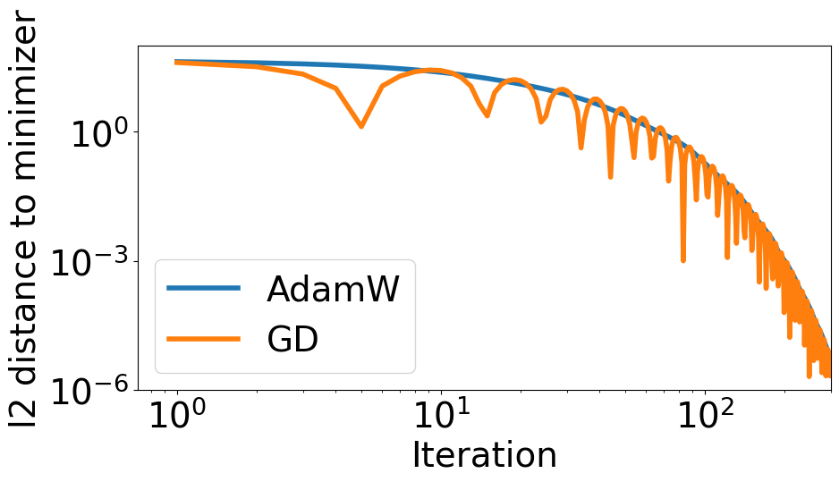
(a) Condition number $1$.

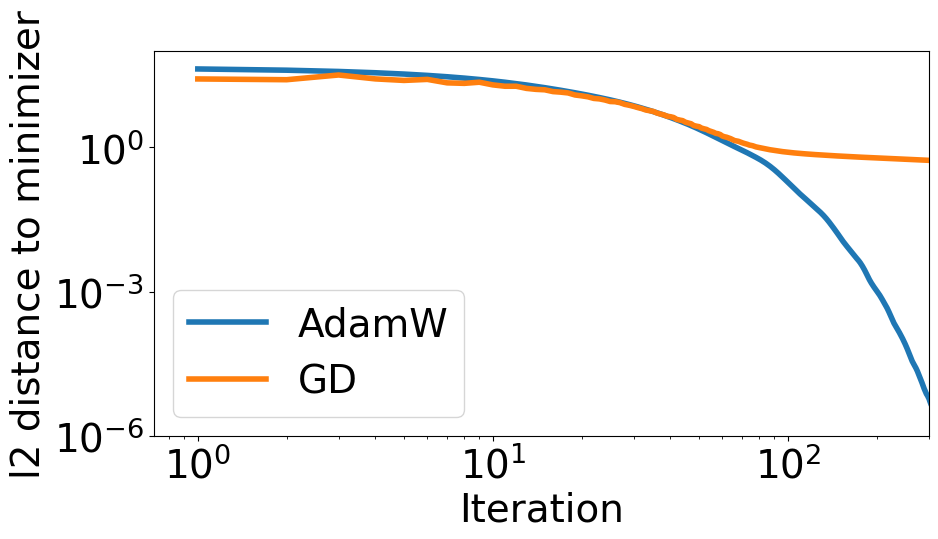
(b) Condition number $100000$.

Figure 1: Non-scale-free GD v.s.  scale-free AdamW on quadratic functions with different condition numbers.

Corollary 1. For quadratic problems $f(\boldsymbol{x})=\tfrac{1}{2}\boldsymbol{x}^{\top}H\boldsymbol{x}+\boldsymbol{b}^{\top}\boldsymbol{x}+c$, with $H$ diagonal and positive definite, any scale-free algorithm will not differentiate between minimizing $f$ and $\tilde{f}(\boldsymbol{x})=\frac{1}{2}\boldsymbol{x}^{\top}\boldsymbol{x}+(H^{-1}\boldsymbol{b})^{\top}\boldsymbol{x}+c$. As the condition number of $\tilde{f}$ is 1, the operation, and most importantly, the convergence, of a scale-free algorithm will not be affected by the condition number of $f$ at all.

Figure 1 illustrates Corollary 1: we compare GD (non-scale-free) with AdamW (scale-free) on optimizing two quadratic functions with the same minimizer, but one’s Hessian matrix being a rescaled version of the other’s, resulting in different condition numbers. The figure clearly shows that, even after tuning the learning rates, the updates of AdamW (starting from the same point) and thus its convergence to the minimizer, is completely unaffected by the condition number, while GD’s updates change drastically and its performance deteriorates significantly when the condition number is large. It is not hard to imagine that such poor training performance would likely also lead to poor testing performance.

This can also explain AdaGrad’s improvements over SGD in certain scenarios. As an additional example, in Appendix B we analyze a variant of AdaGrad with restarts and show an improved convergence on strongly convex functions due to scale-freeness. Note that the folklore justification for such improvements is that the learning rate of AdaGrad approximates the inverse of the Hessian matrix, but this is incorrect: AdaGrad does not compute Hessians and there is no reason to believe it approximates them in general.

More importantly, another scenario demonstrating the advantage of scale-freeness is training deep neural networks. Neural networks are known to suffer from the notorious problem of vanishing/exploding gradients (Bengio et al., 1994; Glorot and Bengio, 2010; Pascanu et al., 2013). This problem leads to the gradient scales being very different across layers, especially between the first and the last layers. The problem is particularly severe when the model is not equipped with normalization mechanisms like Batch Normalization (Ioffe and Szegedy, 2015). In such cases, when using a non-scale-free optimization algorithm (e.g., SGD), the first layers and the last layers will proceed at very different speeds, whereas a scale-free algorithm ensures that each layer is updated at a similar pace. We will investigate these effects empirically in the next section.

4 Deep Learning Empirical Evaluation

In this section, we empirically compare Adam-$\ell_{2}$ with AdamW. First (Section 4.1), we report experiments for deep neural networks on image classification tasks (CIFAR10/100). Here, AdamW enjoys a significant advantage over Adam-$\ell_{2}$ when BN is switched off on deeper neural networks. We also report the correlation between this advantage and the scale-freeness property of AdamW. Next (Section 4.2), we show that AdamW is still almost scale-free even when the $\epsilon$ used in practice is not 0, and how, contrary to AdamW, Adam-$\ell_{2}$ is not scale-free. Finally (Section 4.3), we show that AdamW performs similarly to the update in (7), which we will denote by AdamProx below, thus supporting the observations in Section 3.

Data Normalization and Augmentation: We consider the image classification task on CIFAR-10/100 datasets. Images are normalized per channel using the means and standard deviations computed from all training images. We adopt the data augmentation technique following Lee et al. (2015) (for training only): 4 pixels are padded on each side of an image and a $32\times 32$ crop is randomly sampled from the padded image or its horizontal flip.

Models: For the CIFAR-10 dataset, we employ the Residual Network model (He et al., 2016) of 20/44/56/110/218 layers; and for CIFAR-100, we utilize the DenseNet-BC model (Huang et al., 2017) with 100 layers and a growth-rate of 12. The loss is the cross-entropy loss.

Hyperparameter tuning: For both Adam-$\ell_{2}$ and AdamW, we set $\beta_{1}=0.9$, $\beta_{2}=0.999$, $\epsilon=10^{-8}$ as suggested in the original Adam paper Kingma and Ba (2015). To set the initial step size $\alpha$ and weight decay parameter $\lambda$, we grid search over $\{0.00005,0.0001,0.0005,0.001,0.005\}$ for $\alpha$ and $\{0,0.00001,0.00005,0.0001,0.0005,0.001\}$ for $\lambda$. Whenever the best performing hyperparameters lie in the boundary of the searching grid, we always extend the grid to ensure that the final best-performing hyperparameters fall into the interior of the grid.

Training: For each experiment configuration (e.g., 110-layer Resnet without BN), we randomly select an initialization of the model to use as a fixed starting point for all optimizers and hyperparameter settings. We use a mini-batch of 128, and train 300 epochs unless otherwise specified.

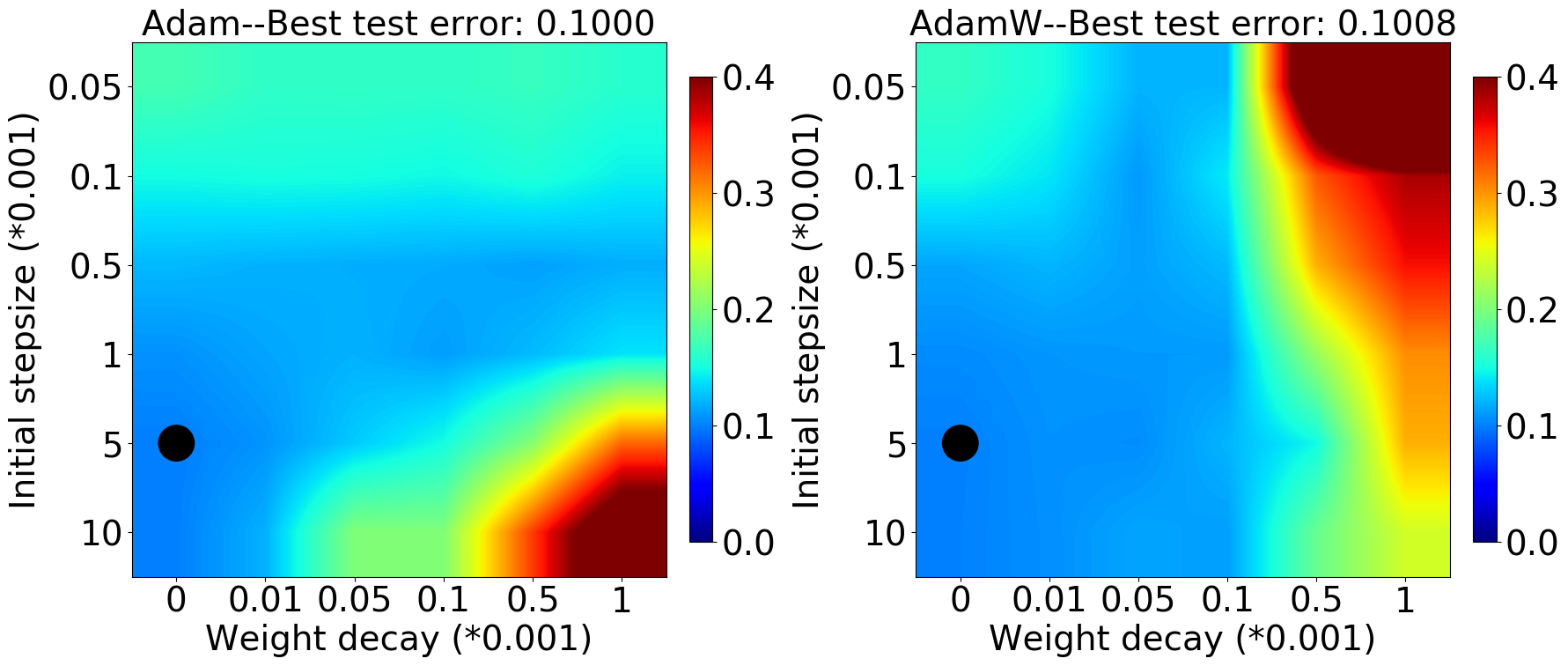
(a) 20 Layer Resnet on CIFAR10

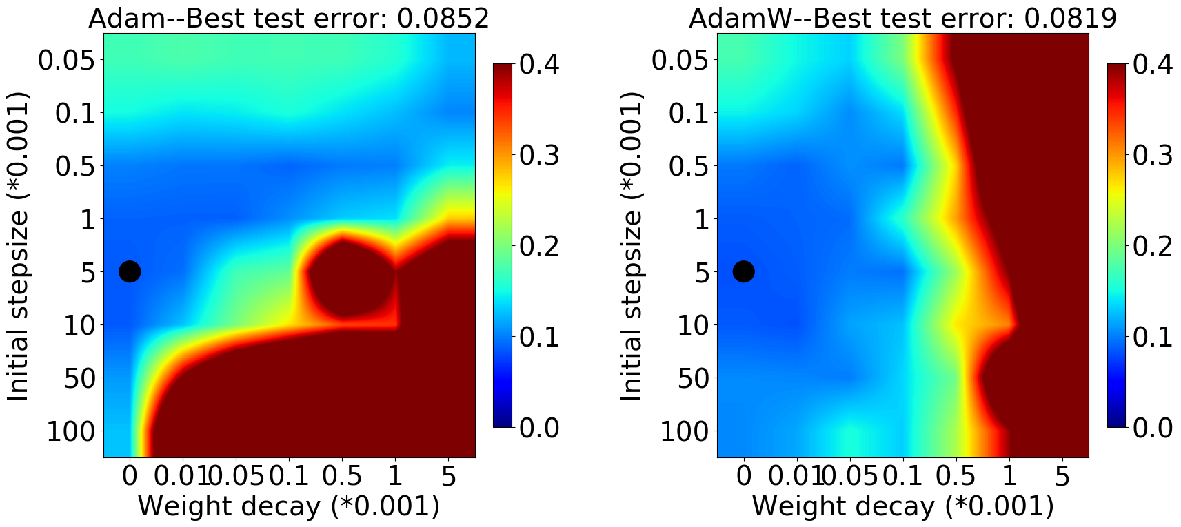
(b) 110 Layer Resnet on CIFAR10

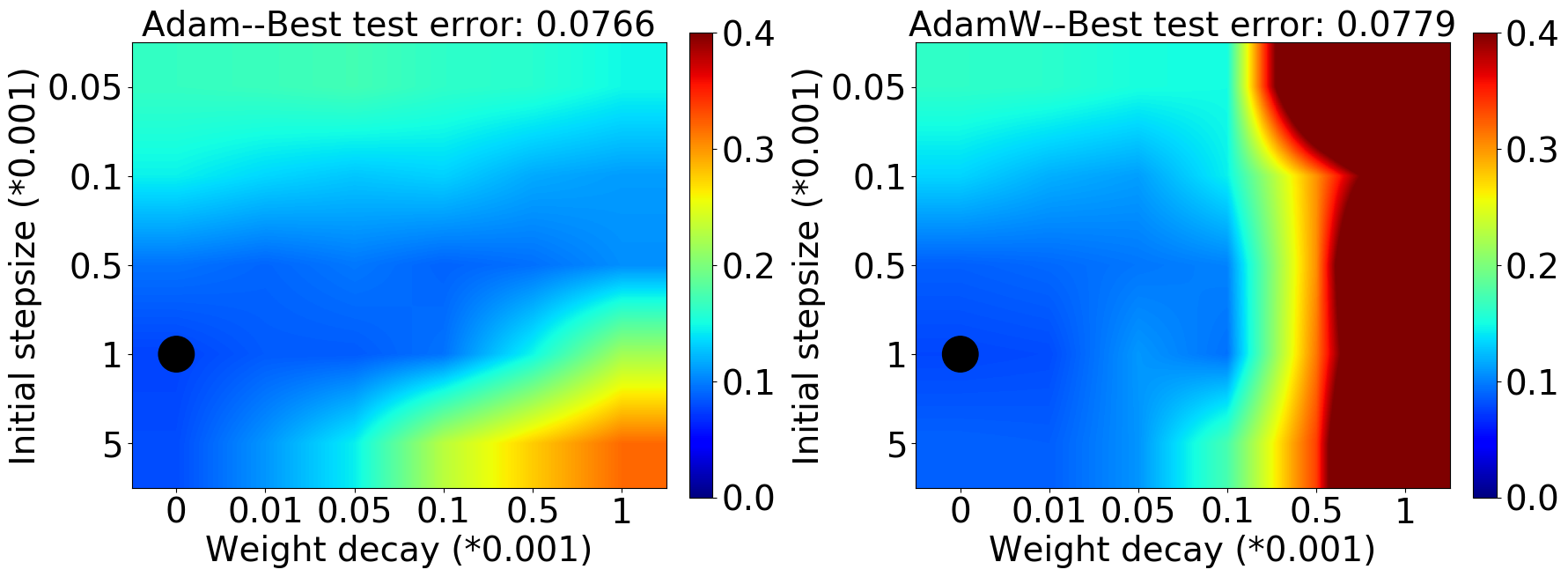
(c) 218 Layer Resnet on CIFAR10

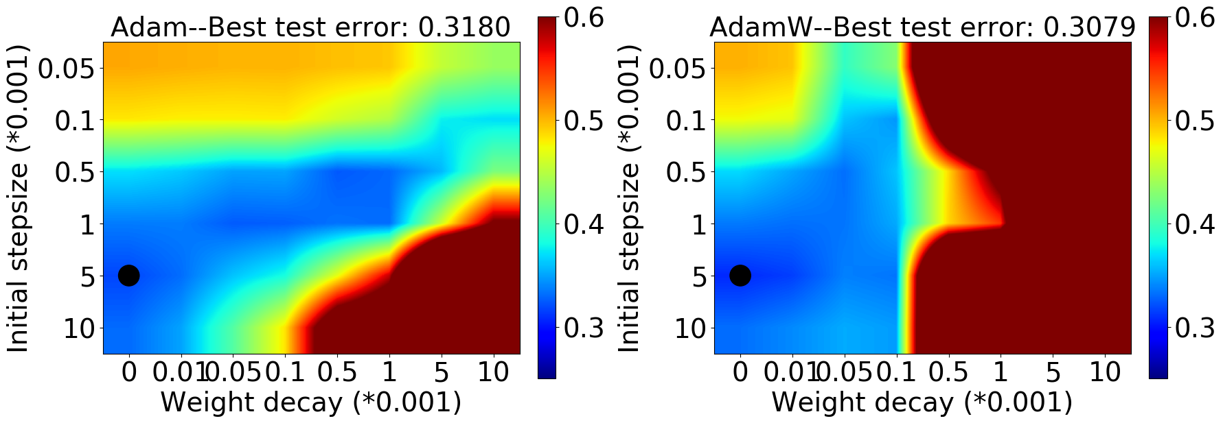
(d) 100 layer DenseNet-BC on CIFAR100

Figure 2: The final Top-1 test error on using AdamW vs. Adam-$\ell_{2}$ on training a Resnet/DenseNet with Batch Normalization on CIFAR10/100 (the black circle denotes the best setting).

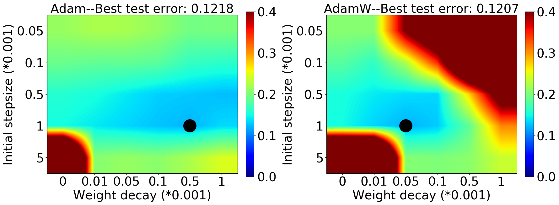
(a) 20 Layer Resnet on CIFAR10

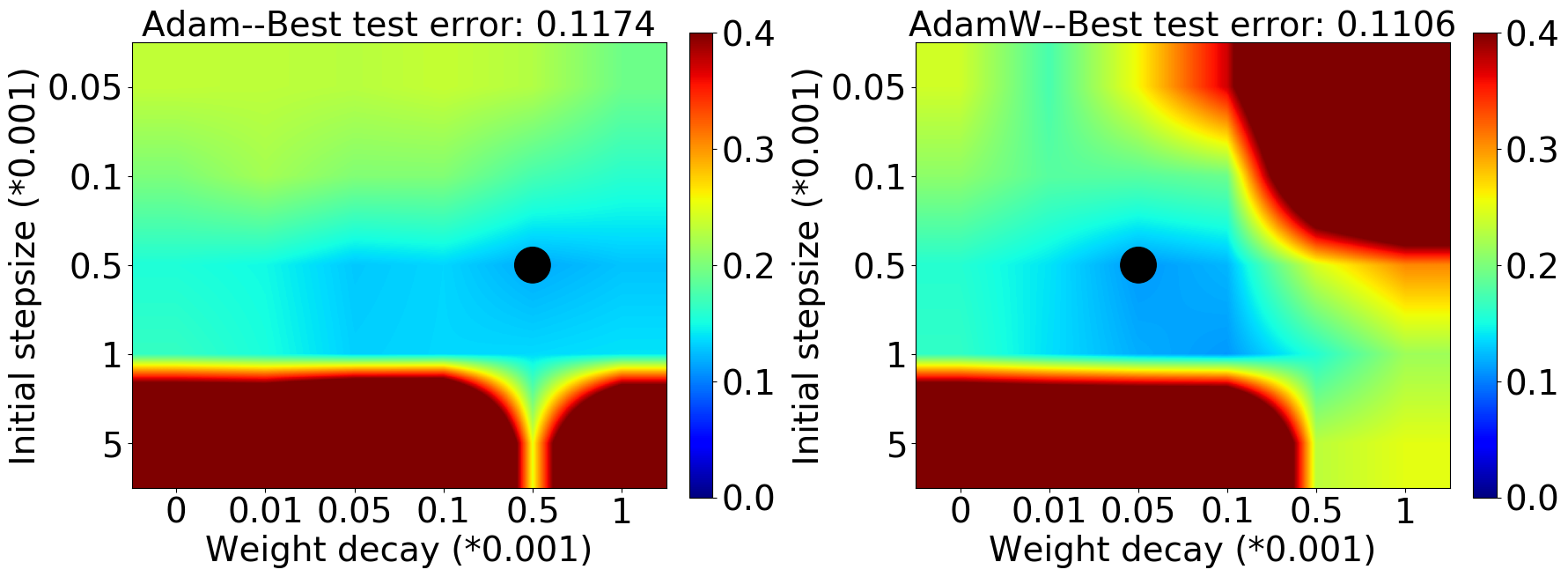
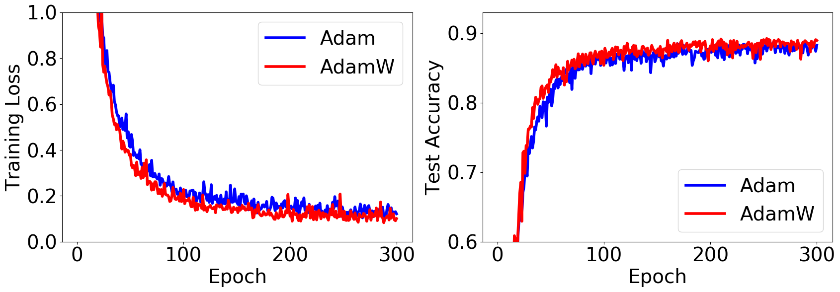
(b) 44 Layer Resnet on CIFAR10

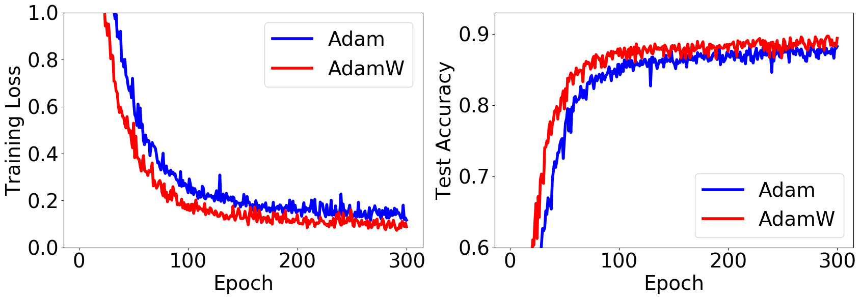
(c) 56 Layer Resnet on CIFAR10

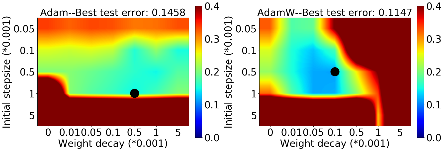
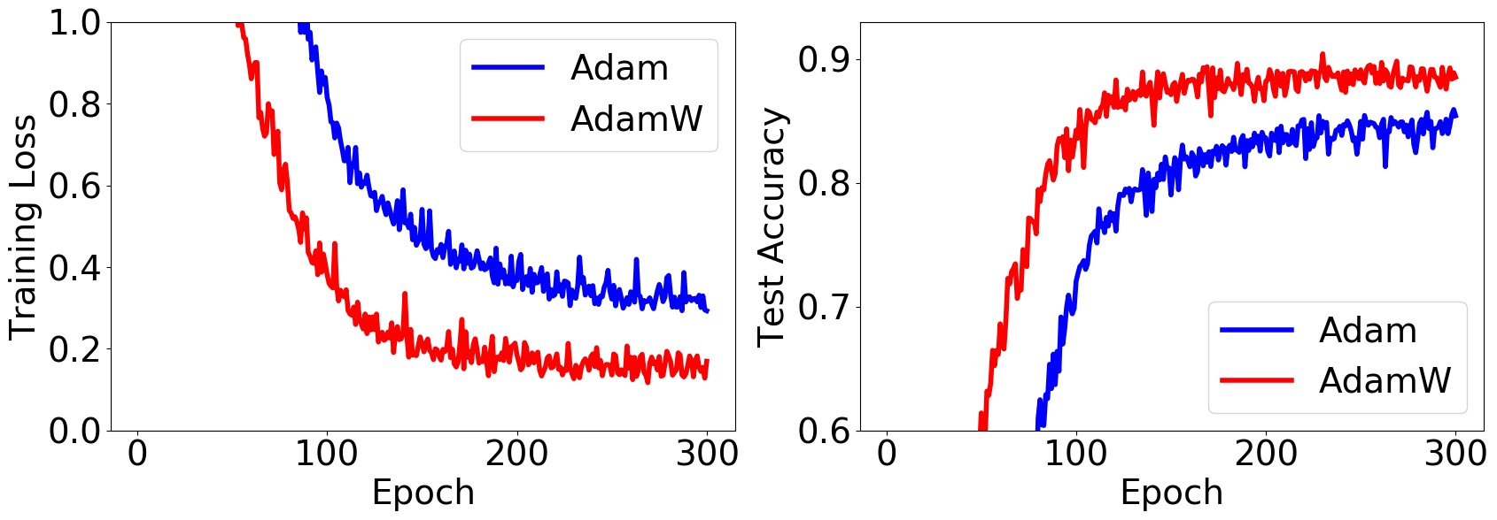
(d) 110 Layer Resnet on CIFAR10

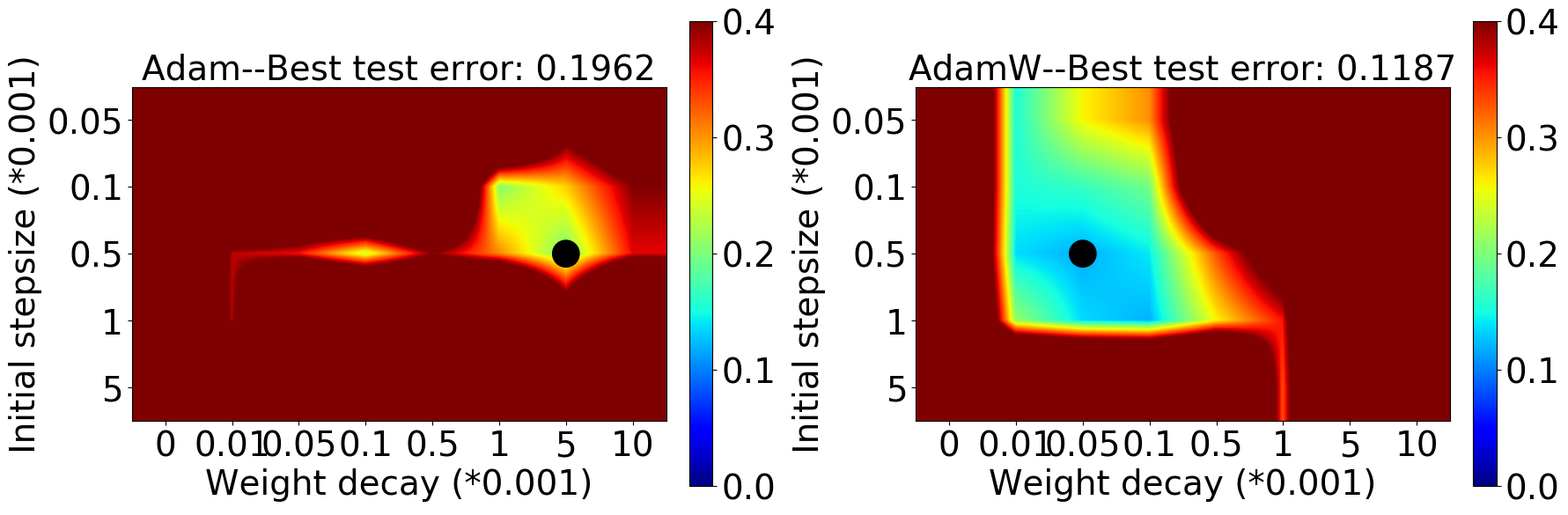
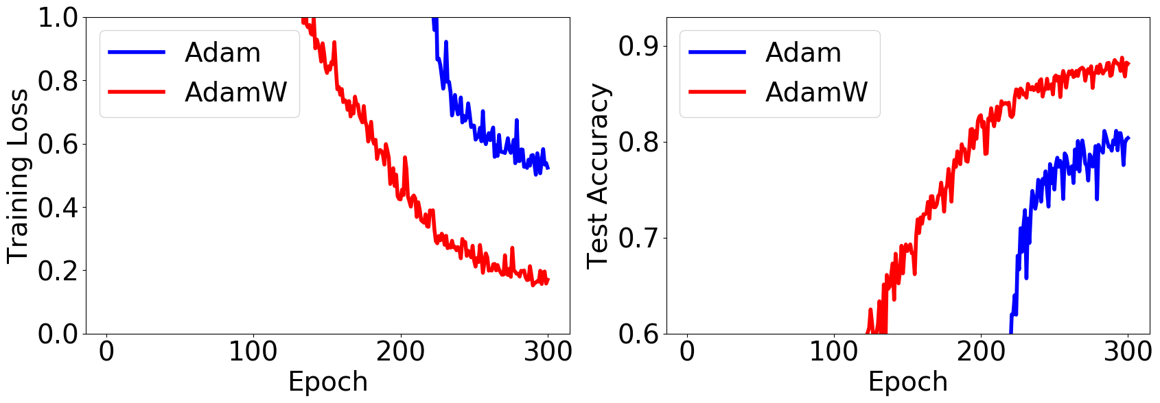
(e) 218 Layer Resnet on CIFAR10

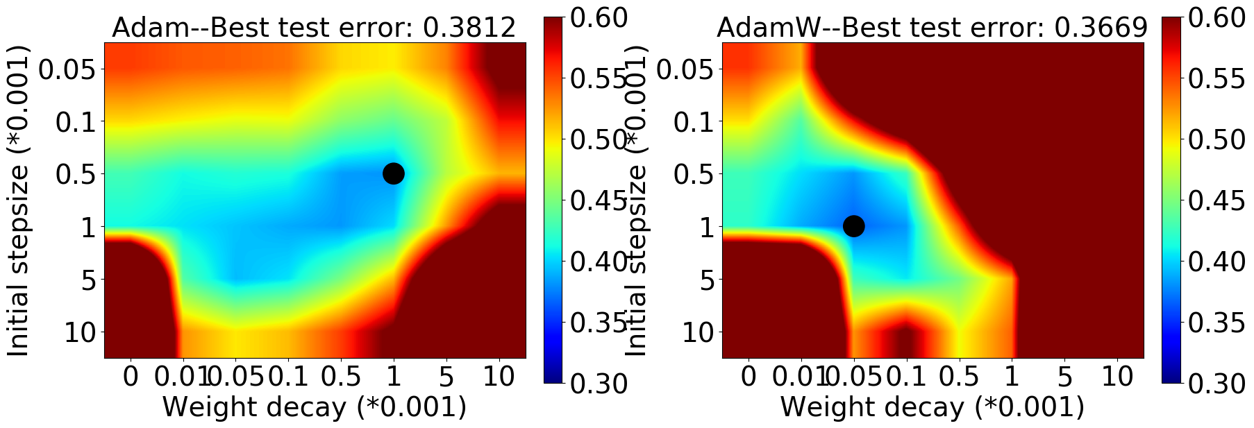
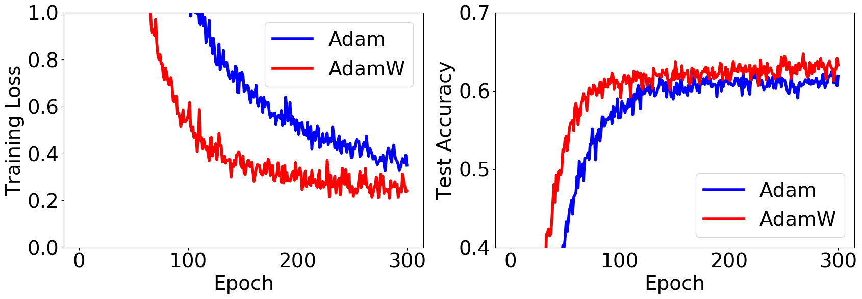
(f) 100 layer DenseNet-BC on CIFAR100

Figure 3: On using AdamW vs. Adam-$\ell_{2}$ on training a Resnet/DenseNet without Batch Normalization on CIFAR10/100. (Left two) The final Top-1 test error (the black circle denotes the best setting). (Middle two) The training loss and test accuracy curve when employing the initial step size and the weight decay parameter that gives the smallest test error. (Right two) The histogram of the magnitude of corresponding updates of all coordinates of the network near the end of the training when employing the initial step size and the weight decay parameter that gives the smallest test error.

4.1 AdamW vs. Adam-$\ell_{2}$: Influence of Batch Normalization and Correlation with Scale-freeness

With BN, Adam-$\ell_{2}$ is on par with AdamW Recently, Bjorck et al. (2020) found that AdamW has no improvement in absolute performance over sufficiently tuned Adam-$\ell_{2}$ in some reinforcement learning experiments. We also discover the same phenomenon in several image classification tasks, see Figure 2. Indeed, the best weight decay parameter is $0$ for all cases and AdamW coincides with Adam-$\ell_{2}$ in these cases. Nevertheless, AdamW does decouple the optimal choice of the weight decay parameter from the initial step size much better than Adam-$\ell_{2}$ in all cases.

Removing BN Notice that the models used in Figure 2 all employ BN. BN works by normalizing the input to each layer across the mini-batch to make each coordinate have zero-mean and unit-variance. Without BN, deep neural networks are known to suffer from gradient explosion and vanishing (Schoenholz et al., 2017). This means each coordinate of the gradient will have very different scales, especially between the first and last layers. For non-scale-free algorithms, the update to the network weights will also be affected and each coordinate will proceed at a different pace. In contrast, scale-free optimizers are robust to such issues as the scaling of any single coordinate will not affect the update. Thus, we consider the case where BN is removed as that is where AdamW and Adam-$\ell_{2}$ will show very different patterns due to scale-freeness.

Without BN, AdamW Outperforms Adam-$\ell_{2}$ In fact, without BN, AdamW outperforms Adam-$\ell_{2}$ even when both are finely tuned, especially on relatively deep neural networks (see Figure 3). AdamW not only obtains a much better test accuracy but also trains much faster.

AdamW’s Advantage and Scale-freeness We also observe that the advantage of AdamW becomes more evident as the network becomes deeper. Recall that as the depth grows, without BN, the gradient explosion and vanishing problem becomes more severe. This means that for the non-scale-free Adam-$\ell_{2}$, the updates of each coordinate will be dispersed on a wider range of scales even when the same weight decay parameter is employed. In contrast, the scales of the updates of AdamW will be much more concentrated in a smaller range. This is exactly verified empirically as illustrated in the 5th & 6th columns of figures in Figure 3. There, we report the histograms of the absolute value of updates of Adam-$\ell_{2}$ vs. AdamW of all coordinates near the end of training (for their comparison over the whole training process please refer to the Appendix C).

This correlation between the advantage of AdamW over Adam-$\ell_{2}$ and the different spread of update scales which is induced by the scale-freeness property of AdamW provides empirical evidence on when AdamW excels over Adam-$\ell_{2}$.

SGD and Scale-freeness The reader might wonder why SGD is known to provide state-of-the-art performance on many deep learning architectures (e.g., He et al., 2016; Huang et al., 2017) without being scale-free. At first blush, this seems to contradict our claims that scale-freeness correlates with good performance. In reality, the good performance of SGD in very deep models is linked to the use of BN that normalizes the gradients. Indeed, we verified empirically that SGD fails spectacularly when BN is not used. For example, on training the 110 layer Resnet without BN using SGD with momentum and weight decay of $0.0001$, even a learning rate of $1e-10$ will lead to divergence.

4.2 Verifying Scale-Freeness

In the previous section, we elaborated on the scale-freeness property of AdamW and its correlation with AdamW’s advantage over Adam-$\ell_{2}$. However, one may notice that in practice, the $\epsilon$ factor in the AdamW update is typically small but not 0, in our case $1e$-$8$, thus preventing it from completely scale-free. In this section, we verify that the effect of such an $\epsilon$ on the scale-freeness is negligible.

As a simple empirical verification of the scale-freeness, we consider the scenario where we multiply the loss function by a positive number. Note that any other method to test scale-freeness would be equally good. For a feed-forward neural network without BN, this means the gradient would also be scaled up by that factor. In this case, the updates of a scale-free optimization algorithm would remain exactly the same, whereas they would change for an optimization algorithm that is not scale-free.

Figure 4 shows results of the loss function being multiplied by 10 and 100 respectively on optimizing a 110-layer Resnet with BN removed. For results of the original loss see Figure 3(d). We can see that AdamW has almost the same performance across the range of initial learning rates and weight decay parameters, and most importantly, the best values of these two hyperparameters remain the same. This verifies that, even when employing a (small) non-zero $\epsilon$, AdamW is still approximately scale-free. In contrast, Adam-$\ell_{2}$ is not scale-free and we can see that its behavior varies drastically with the best initial learning rates and weight decay parameters in each setting totally different.

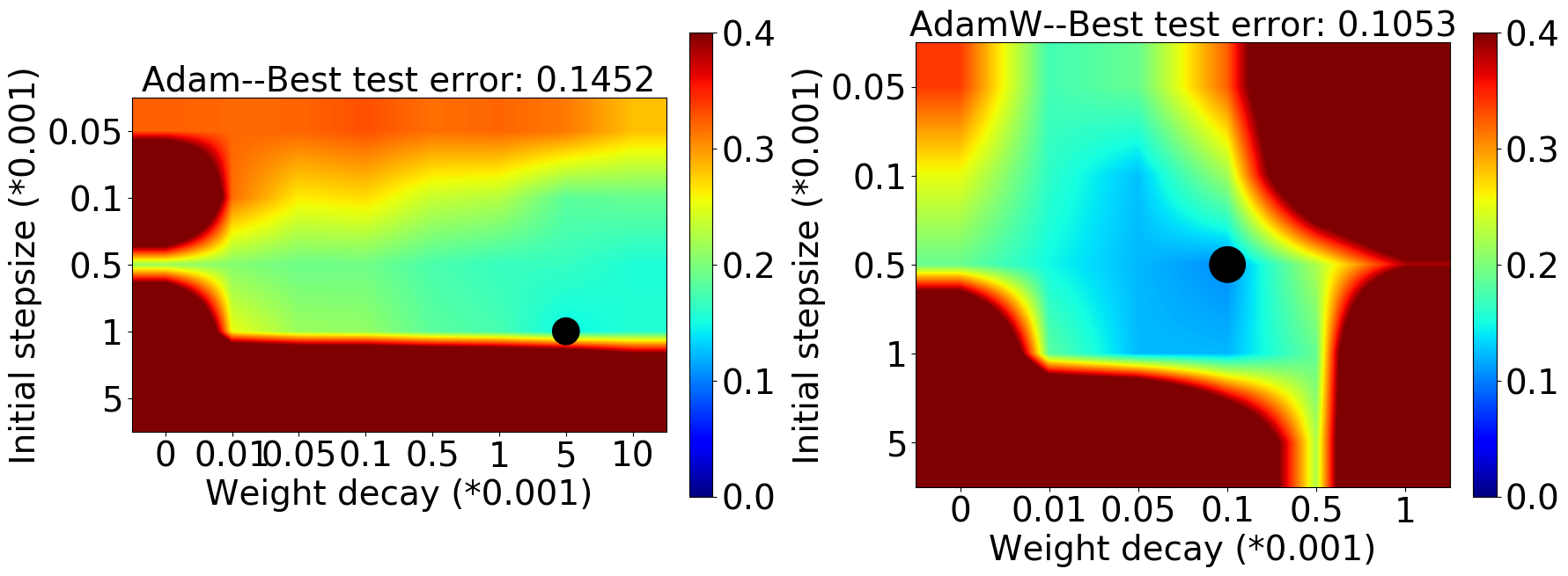
(a) Loss multiplied by 10

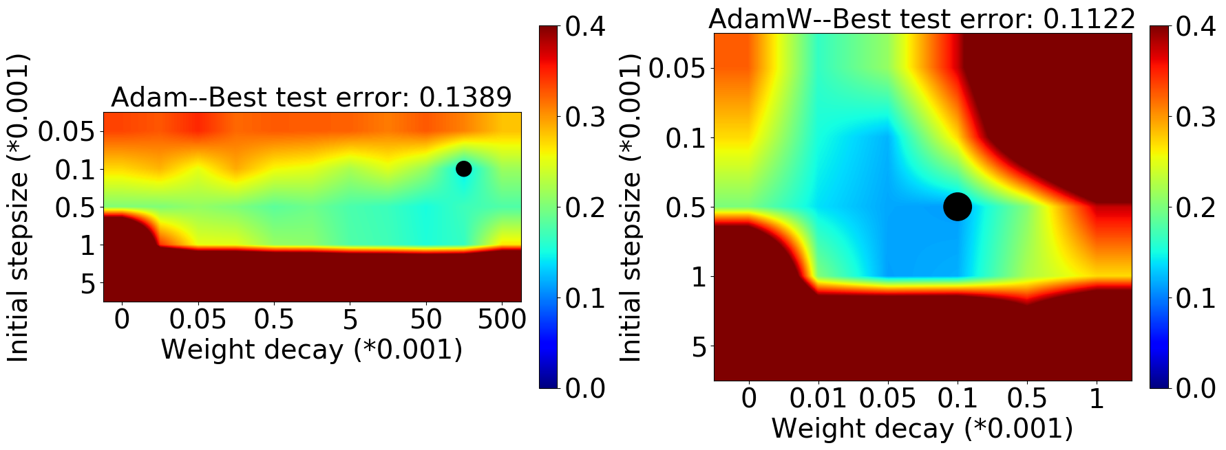
(b) Loss multiplied by 100

Figure 4: The final top-1 test error of AdamW vs. Adam-$\ell_{2}$ on optimizing a 110-layer Resnet with BN removed on CIFAR-10 with the loss function multiplied by 10 (left two figures) and 100 (right two figures).

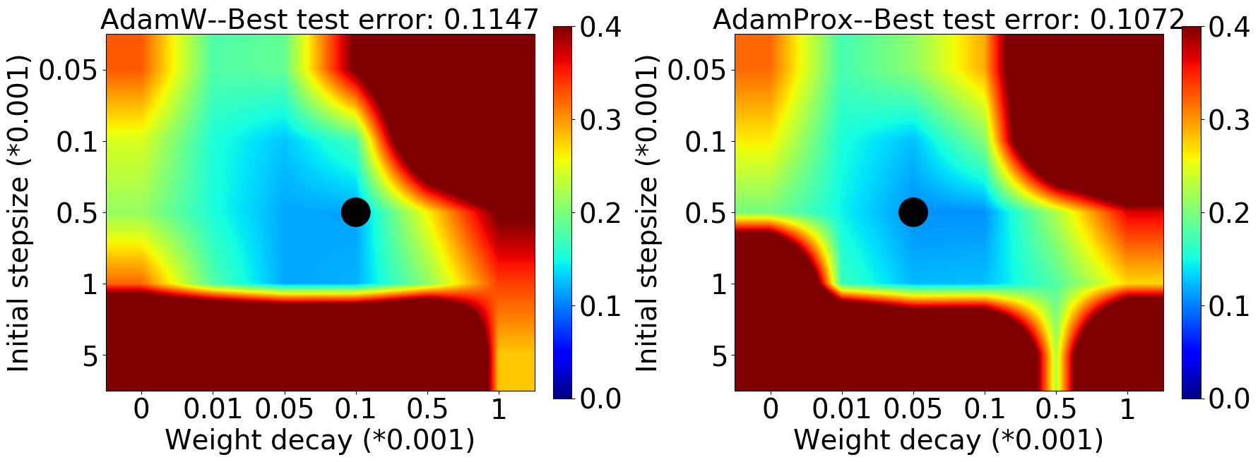
(a) ResNet on CIFAR-10

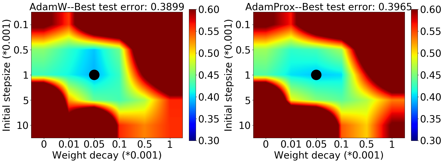
(b) DenseNet-BC on CIFAR-100

Figure 5: The final Top-1 test error of using AdamW vs. AdamProx on training (the black circle denotes the best setting). (Top row) a 110-layer ResNet with BN removed on CIFAR-10 (trained for 300 epochs). (Bottom row) a 100-layer DenseNet-BC with BN removed on CIFAR-100 (trained for 100 epochs).

4.3 AdamW and AdamProx Behave very Similarly

In Section 3, we showed theoretically that AdamW is the first order Taylor approximation of AdamProx (update rule (7)). Beyond this theoretical argument, here we verify empirically that the approximation is good. In Figure 5, we consider the case when $\eta_{t}$ = 1 for all $t$ - a relatively large constant learning rate schedule. In such cases, AdamW and AdamProx still behave very similarly. This suggests that for most learning rate schedules, e.g., cosine, exponential, polynomial, and step decay, which all monotonously decrease from $\eta_{0}=1$, AdamProx will remain a very good approximation to AdamW. Thus, it is reasonable to use the more classically-linked AdamProx to try to understand AdamW.

5 Conclusion and Future Works

In this paper, we provide insights for understanding the merits of AdamW from two points of view. We first show that AdamW is an approximation of the proximal updates both theoretically and empirically. We then identify the setting of training very deep neural networks without batch normalization in which AdamW substantially outperforms Adam-$\ell_{2}$ in both training and testing and show its correlation with the scale-freeness property of AdamW. Nevertheless, we are aware of some limitations of this work as well as many directions worth exploring.

Limitations First, we only focus on investigating the effects of scale-freeness on Adam-$\ell_{2}$ and AdamW, but it would be interesting to study scale-freeness more generally. Also, what we showed is just a correlation instead of causality thus we did not rule out other possible causes beyond scale-freeness for the success of AdamW. Indeed, rigorously proving causality for any such claim is extremely difficult - even in the hard sciences. Note that there are papers claiming that adaptive updates have worse generalization (Wilson et al., 2017); however, such claims have been recently partly confuted (see, e.g., Agarwal et al., 2020). On this note, despite its empirical success, we stress that Adam will not even converge on some convex functions (Reddi et al., 2018), thus making it hard to prove formal theoretical convergence and/or generalization guarantees.

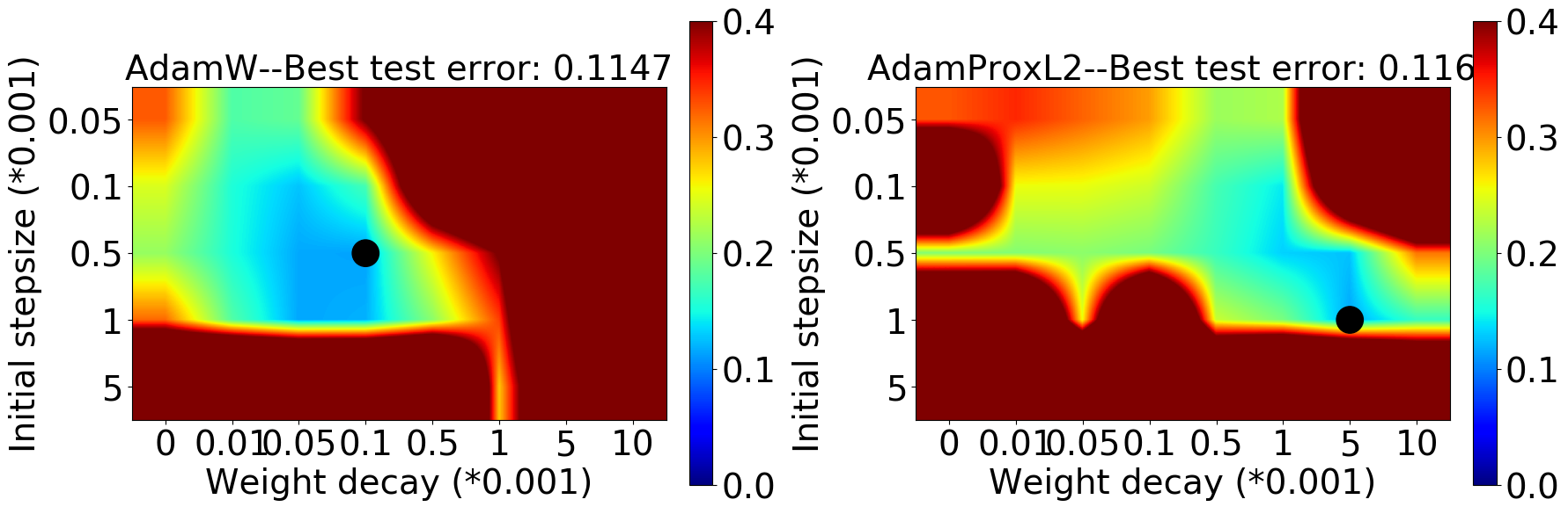
Figure 6: Final Top-1 test error of using AdamW vs. AdamProxL2 to train a 110-layer ResNet without BN on CIFAR10 (the black circle denotes the best setting).

Update for no-square $\ell_{2}$ regularization. Instead of using the squared $\ell_{2}$ regularization, we might think to use the $\ell_{2}$ regularization, that is without the square. This is known to have better statistical properties than the squared $\ell_{2}$ (Orabona, 2014), but it is not smooth so it is harder to be optimized. However, with proximal updates, we don’t have to worry about its non-smoothness. Hence, we can consider the objective function $F(\boldsymbol{x})=\lambda\|\boldsymbol{x}\|_{2}+f(\boldsymbol{x})$.

The corresponding prox-SGD update was derived in Duchi and Singer (2009) for scalar learning rates and it is easy to see that it generalizes to our setting for $M_{t}=\eta_{t}I_{d}$ as

$$\boldsymbol{x}_{t+1}=\max\left(1-\tfrac{\lambda\eta_{t}}{\|\boldsymbol{x}_{t}-\eta_{t}\boldsymbol{p}_{t}\|},0\right)(\boldsymbol{x}_{t}-\eta_{t}\boldsymbol{p}_{t})~{}.$$

Its performance, named AdamProxL2, as shown in Figure 6, can be on a par with AdamW.

Distributed Training Batch normalization is not user-friendly in distributed training as it requires each machine to collect a batch of statistics to update the model which may be inaccurate when machines do not communicate frequently with each other Goyal et al. (2017). Since AdamW outperforms Adam-$\ell_{2}$ significantly in settings without BN, at least in feed-forward neural networks, we can apply AdamW in distributed training to see if it still enjoys the same merits.

Appendices

Appendix A Proof of Theorem 3.1

Proof.

From the Fundamental Theorem of Calculus we have:

$$\nabla f(\boldsymbol{x})=\nabla f(\boldsymbol{x}^{*})+\int^{1}_{0}\nabla^{2}f(\boldsymbol{x}^{*}+t(\boldsymbol{x}-\boldsymbol{x}^{*}))(\boldsymbol{x}-\boldsymbol{x}^{*})dt=\int^{1}_{0}\nabla^{2}f(\boldsymbol{x}^{*}+t(\boldsymbol{x}-\boldsymbol{x}^{*}))(\boldsymbol{x}-\boldsymbol{x}^{*})dt~{}.$$ (8)

Thus, for any function $\tilde{f}_{\Lambda}(\boldsymbol{x})$ whose Hessian is $\Lambda\nabla^{2}f(\boldsymbol{x})$ and $\nabla\tilde{f}_{\Lambda}(\boldsymbol{x}^{*})=0$, we have $\nabla\tilde{f}_{\Lambda}(\boldsymbol{x})=\Lambda\nabla f(\boldsymbol{x})$.

Now, from the definition of a scale-free algorithm, the iterates of such an algorithm do not change when one multiplies each coordinate of all the gradients by a positive constant. Thus, a scale-free algorithm optimizing $f$ behaves the same as if it is optimizing $\tilde{f}_{\Lambda}$. ∎

Appendix B A Scale-free Algorithm with Dependency on the Condition Number

Algorithm 2 AdaGrad (Duchi et al., 2011; McMahan and Streeter, 2010) (All operations on vectors are element-wise.)

  Input: #Iterations $T$, a set $\mathcal{K}$, $\boldsymbol{x}_{1}\in\mathcal{K}$, stepsize $\eta$

  for $t=1\ldots T$  do

     Receive: $\nabla f(\boldsymbol{x}_{t})$

     Set: $\boldsymbol{\eta}_{t}=\frac{\eta}{\sqrt{\sum^{t}_{i=1}(\nabla f(\boldsymbol{x}_{i}))^{2}}}$

     Update: $\boldsymbol{x}_{t+1}=\Pi_{\mathcal{K}}\left(\boldsymbol{x}_{t}-\boldsymbol{\eta}_{t}\nabla f(\boldsymbol{x}_{t})\right)$ where $\Pi_{\mathcal{K}}$ is the projection onto $\mathcal{K}$.

  end for

  Output: $\bar{\boldsymbol{x}}=\frac{1}{T}\sum^{T}_{t=1}\boldsymbol{x}_{t}$.

Algorithm 3 AdaGrad with Restart

  Input: #Rounds $N$, $\boldsymbol{x}_{0}\in\mathbb{R}^{d}$, upper bound on $\|\boldsymbol{x}_{0}-\boldsymbol{x}^{*}\|_{\infty}$ as $D_{\infty}$, strong convexity $\mu$, smoothness $M$

  Set: $\bar{\boldsymbol{x}}_{0}=\boldsymbol{x}_{0}$

  for $i=1\ldots N$  do

     Run Algorithm 2 to get $\bar{\boldsymbol{x}}_{i}$ with $T=32d\frac{M}{\mu}$, $\boldsymbol{x}_{1}=\bar{\boldsymbol{x}}_{i-1}$, $\mathcal{K}=\{\boldsymbol{x}:\|\boldsymbol{x}-\bar{\boldsymbol{x}}_{i-1}\|_{\infty}^{2}\leq\frac{D_{\infty}^{2}}{4^{i-1}}\}$, $\eta=\frac{D_{\infty}/\sqrt{2}}{2^{i-1}}$

  end for

  Output: $\bar{\boldsymbol{x}}_{N}$.

Theorem B.1.

Let $\mathcal{K}$ be a hypercube with $\|\boldsymbol{x}-\boldsymbol{y}\|_{\infty}\leq D_{\infty}$ for any $\boldsymbol{x},\boldsymbol{y}\in\mathcal{K}$. For a convex function $f$, set $\eta=\frac{D_{\infty}}{\sqrt{2}}$, then Algorithm 2 guarantees for any $\boldsymbol{x}\in\mathcal{K}$:

$$\sum_{t=1}^{T}f(\boldsymbol{x}_{t})-f(\boldsymbol{x})\leq\sqrt{2dD_{\infty}^{2}\sum_{t=1}^{T}\|\nabla f(\boldsymbol{x}_{t})\|^{2}}~{}.$$ (9)

Theorem B.2.

For a $\mu$ strongly convex and $M$ smooth function $f$, denote its unique minimizer as $\boldsymbol{x}^{*}\in\mathbb{R}^{d}$. Given $\boldsymbol{x}_{0}\in\mathbb{R}^{d}$, assume that $\|\boldsymbol{x}_{0}-\boldsymbol{x}^{*}\|_{\infty}\leq D_{\infty}$, then Algorithm 3 guarantees:

$$\|\bar{\boldsymbol{x}}_{N}-\boldsymbol{x}^{*}\|_{\infty}^{2}\leq\frac{D_{\infty}^{2}}{4^{N}}~{}.$$ (10)

Thus, to get a $\boldsymbol{x}$ such that $\|\boldsymbol{x}-\boldsymbol{x}^{*}\|_{\infty}^{2}\leq\epsilon$, we need at most $32d\frac{M}{\mu}\log_{4}\left({D_{\infty}^{2}}/{\epsilon}\right)$ gradient calls.

Proof of Theorem B.2.

Consider round $i$ and assume $\mathcal{K}$ passed to Algorithm 2 is bounded w.r.t. $\ell_{\infty}$ norm by $D_{\infty_{i}}$. When $f$ is $\mu$-strongly convex and $M$ smooth, let $\boldsymbol{x}=\boldsymbol{x}^{*}$, Equation (9) becomes:

$$\sum_{t=1}^{T}f(\boldsymbol{x}_{t})-f(\boldsymbol{x}^{*})\leq\sqrt{2dD_{\infty_{i}}^{2}\sum_{t=1}^{T}\|\nabla f(\boldsymbol{x}_{t})\|^{2}}\leq\sqrt{4MdD_{\infty_{i}}^{2}\sum_{t=1}^{T}(f(\boldsymbol{x}_{t})-f(\boldsymbol{x}^{*}))}~{},$$ (11)

where the second inequality is by the $M$ smoothness of $f$. This gives:

$$\sum_{t=1}^{T}f(\boldsymbol{x}_{t})-f(\boldsymbol{x}^{*})\leq 4MdD_{\infty_{i}}^{2}~{}.$$ (12)

Let $\bar{\boldsymbol{x}}_{i}=\frac{1}{T}\sum^{T}_{t=1}\boldsymbol{x}_{t}$ we have by the $\mu$-strong-convexity that:

$$\|\bar{\boldsymbol{x}}_{i}-\boldsymbol{x}^{*}\|_{\infty}^{2}\leq\|\bar{\boldsymbol{x}}_{i}-\boldsymbol{x}^{*}\|^{2}\leq\frac{2}{\mu}(f(\bar{\boldsymbol{x}})-f(\boldsymbol{x}^{*}))\leq\frac{2}{\mu}\frac{1}{T}\sum^{T}_{t=1}(f(\boldsymbol{x}_{t})-f(\boldsymbol{x}^{*}))\leq\frac{8MdD_{\infty_{i}}^{2}}{\mu T}~{}.$$ (13)

Put $T=32d\frac{M}{\mu}$ in Equation (13) we have that $\|\bar{\boldsymbol{x}}_{i}-\boldsymbol{x}^{*}\|_{\infty}^{2}\leq\frac{D_{\infty_{i}}^{2}}{4}$. Thus, after each round, the $\ell_{\infty}$ distance between the update $\bar{\boldsymbol{x}}_{i}$ and $\boldsymbol{x}^{*}$ is shrinked by half, which in turn ensures that $\boldsymbol{x}^{*}$ is still inside the $\mathcal{K}$ passed to Algorithm 2 in the next round with $D_{\infty_{i+1}}=\frac{D_{\infty_{i}}}{2}$. This concludes the proof. ∎

Proof of Theorem B.1.

$$\sum^{T}_{t=1}f(\boldsymbol{x}_{t})-f(\boldsymbol{x})$$ (14)

$$\leq\sum^{T}_{t=1}\langle\nabla f(\boldsymbol{x}_{t}),\boldsymbol{x}_{t}-\boldsymbol{x}\rangle$$ (15)

$$=\sum^{T}_{t=1}\sum^{d}_{j=1}\frac{\partial f}{\partial x_{t,j}}(\boldsymbol{x}_{t})*(x_{t,j}-x_{j})$$ (16)

$$=\sum^{T}_{t=1}\sum^{d}_{j=1}\frac{(x_{t,j}-x_{j})^{2}-\left(x_{t,j}-\eta_{t,j}\frac{\partial f}{\partial x_{t,j}}(\boldsymbol{x}_{t})-x_{j}\right)^{2}}{2\eta_{t,j}}+\sum^{T}_{t=1}\sum^{d}_{j=1}\frac{\eta_{t,j}}{2}\left(\frac{\partial f}{\partial x_{t,j}}(\boldsymbol{x}_{t})\right)^{2}$$ (17)

$$\leq\sum^{T}_{t=1}\sum^{d}_{j=1}\frac{(x_{t,j}-x_{j})^{2}-(x_{t+1,j}-x_{j})^{2}}{2\eta_{t,j}}+\sum^{T}_{t=1}\sum^{d}_{j=1}\frac{\eta_{t,j}}{2}\left(\frac{\partial f}{\partial x_{t,j}}(\boldsymbol{x}_{t})\right)^{2}$$ (18)

$$\leq\sum^{d}_{j=1}\sum^{T}_{t=1}\frac{(x_{t,j}-x_{j})^{2}}{2}\left(\frac{1}{\eta_{t,j}}-\frac{1}{\eta_{t-1,j}}\right)+\sum^{d}_{j=1}\sum^{T}_{t=1}\frac{\eta_{t,j}}{2}\left(\frac{\partial f}{\partial x_{t,j}}(\boldsymbol{x}_{t})\right)^{2}$$ (19)

$$\leq\frac{D_{\infty}^{2}}{2\eta}\sum^{d}_{j=1}\sum^{T}_{t=1}\left(\sqrt{\sum^{t}_{i=1}\left(\frac{\partial f}{\partial x_{i,j}}(\boldsymbol{x}_{i})\right)^{2}}-\sqrt{\sum^{t-1}_{i=1}\left(\frac{\partial f}{\partial x_{i,j}}(\boldsymbol{x}_{i})\right)^{2}}\right)+\sum^{d}_{j=1}\sum^{T}_{t=1}\frac{\eta}{2\sqrt{\sum^{t}_{i=1}\left(\frac{\partial f}{\partial x_{i,j}}(\boldsymbol{x}_{i})\right)^{2}}}\left(\frac{\partial f}{\partial x_{t,j}}(\boldsymbol{x}_{t})\right)^{2}$$ (20)

$$\leq\sum^{d}_{j=1}\left(\frac{D_{\infty}^{2}}{2\eta}\sqrt{\sum^{T}_{t=1}\left(\frac{\partial f}{\partial x_{t,j}}(\boldsymbol{x}_{t})\right)^{2}}+\eta\sqrt{\sum^{T}_{t=1}\left(\frac{\partial f}{\partial x_{t,j}}(\boldsymbol{x}_{t})\right)^{2}}\right)$$ (21)

$$=\sum^{d}_{j=1}\sqrt{2D_{\infty}^{2}\sum^{T}_{t=1}\left(\frac{\partial f}{\partial x_{t,j}}(\boldsymbol{x}_{t})\right)^{2}}$$ (22)

$$\leq\sqrt{2dD_{\infty}^{2}\sum^{T}_{t=1}\sum^{d}_{j=1}\left(\frac{\partial f}{\partial x_{t,j}}(\boldsymbol{x}_{t})\right)^{2}}$$ (23)

$$=\sqrt{2dD_{\infty}^{2}\sum^{T}_{t=1}\|\nabla f(\boldsymbol{x}_{t}))\|^{2}}~{}.$$ (24)

where the first inequality is by convexity, the second one by the projection lemma as the projection onto a hypercube equals performing the projection independently for each coordinate, the fifth one by Lemma 5 in (McMahan and Streeter, 2010), and the last one by the concavity of $\sqrt{\cdot}$. ∎

Appendix C The Histograms of the Magnitude of each Update Coordinate during the Entire Training Phase

In this section, we report the histograms of the absolute value of updates of Adam-$\ell_{2}$ vs. AdamW of all coordinates divided by $\alpha$ during the whole training process. From the figures shown below, we can clearly see that AdamW’s updates remain in a much more concentrated scale range than Adam-$\ell_{2}$ during the entire training. Moreover, as the depth of the network grows, Adam-$\ell_{2}$’s updates become more and more dispersed, while AdamW’s updates are still concentrated. (Note that the leftmost bin contains all values equal to or less than $2^{-27}\approx 10^{-8.1}$ and the rightmost bin contains all values equal to or larger than $1$.)

(a) Adam-$\ell_{2}$

(b) AdamW

Figure 7: The histograms of the magnitudes of all updates (without $\alpha$) of a 20-layer Resnet with BN removed trained by AdamW or Adam-$\ell_{2}$ on CIFAR10.

(a) Adam-$\ell_{2}$

(b) AdamW

Figure 8: The histograms of the magnitudes of all updates (without $\alpha$) of a 44-layer Resnet with BN removed trained by AdamW or Adam-$\ell_{2}$ on CIFAR10.

(a) Adam-$\ell_{2}$

(b) AdamW

Figure 9: The histograms of the magnitudes of all updates (without $\alpha$) of a 56-layer Resnet with BN removed trained by AdamW or Adam-$\ell_{2}$ on CIFAR10.

(a) Adam-$\ell_{2}$

(b) AdamW

Figure 10: The histograms of the magnitudes of all updates (without $\alpha$) of a 110-layer Resnet with BN removed trained by AdamW or Adam-$\ell_{2}$ on CIFAR10.

(a) Adam-$\ell_{2}$

(b) AdamW

Figure 11: The histograms of the magnitudes of all updates (without $\alpha$) of a 218-layer Resnet with BN removed trained by AdamW or Adam-$\ell_{2}$ on CIFAR10.

(a) Adam-$\ell_{2}$

(b) AdamW

Figure 12: The histograms of the magnitudes of all updates (without $\alpha$) of a 100-layer DenseNet-BC with BN removed trained by AdamW or Adam-$\ell_{2}$ on CIFAR100.

References

- Agarwal et al. (2020) N. Agarwal, R. Anil, E. Hazan, T. Koren, and C. Zhang. Disentangling adaptive gradient methods from learning rates. arXiv preprint arXiv:2002.11803, 2020.
- Asi and Duchi (2019) H. Asi and J. C. Duchi. Stochastic (approximate) proximal point methods: Convergence, optimality, and adaptivity. SIAM Journal on Optimization, 29(3):2257–2290, 2019.
- Ba et al. (2016) J. L. Ba, J. R. Kiros, and G. E. Hinton. Layer normalization. arXiv preprint arXiv:1607.06450, 2016.
- Beck and Teboulle (2003) A. Beck and M. Teboulle. Mirror descent and nonlinear projected subgradient methods for convex optimization. Operations Research Letters, 31(3):167–175, 2003.
- Bengio et al. (1994) Y. Bengio, P. Simard, and P. Frasconi. Learning long-term dependencies with gradient descent is difficult. IEEE transactions on neural networks, 5(2):157–166, 1994.
- Bjorck et al. (2020) J. Bjorck, K. Q. Weinberger, and C. P. Gomes. Understanding decoupled and early weight decay. ArXiv, abs/2012.13841, 2020.
- Bos and Chug (1996) S. Bos and E. Chug. Using weight decay to optimize the generalization ability of a perceptron. Proceedings of International Conference on Neural Networks (ICNN’96), 1:241–246 vol.1, 1996.
- Boyd and Vandenberghe (2004) S. Boyd and L. Vandenberghe. Convex Optimization. Cambridge University Press, New York, NY, USA, 2004. ISBN 0521833787.
- Brock et al. (2021) A. Brock, S. De, S. L. Smith, and K. Simonyan. High-performance large-scale image recognition without normalization. In Proc. of the International Conference on Machine Learning (ICML), pages 1059–1071, 2021.
- Bulò et al. (2018) S. R. Bulò, L. Porzi, and P. Kontschieder. In-place activated BatchNorm for memory-optimized training of DNNs. In Proceedings of the IEEE Conference on Computer Vision and Pattern Recognition, pages 5639–5647, 2018.
- Carion et al. (2020) N. Carion, F. Massa, G. Synnaeve, N. Usunier, A. Kirillov, and S. Zagoruyko. End-to-end object detection with transformers. In European Conference on Computer Vision, pages 213–229. Springer, 2020.
- Cesa-Bianchi et al. (2007) N. Cesa-Bianchi, Y. Mansour, and G. Stoltz. Improved second-order bounds for prediction with expert advice. Machine Learning, 66(2):321–352, 2007.
- Chen et al. (2020) T. Chen, S. Kornblith, M. Norouzi, and G. Hinton. A simple framework for contrastive learning of visual representations. In Hal Daumé, III and Aarti Singh, editors, Proceedings of the 37th International Conference on Machine Learning, volume 119 of Proceedings of Machine Learning Research, pages 1597–1607. PMLR, 13–18 Jul 2020.
- De and Smith (2020) S. De and S. Smith. Batch normalization biases residual blocks towards the identity function in deep networks. Advances in Neural Information Processing Systems, 33, 2020.
- Devlin et al. (2019) J. Devlin, Ming-Wei Chang, Kenton Lee, and Kristina Toutanova. BERT: Pre-training of deep bidirectional transformers for language understanding. In NAACL-HLT, 2019.
- Dosovitskiy et al. (2021) A. Dosovitskiy, L. Beyer, A. Kolesnikov, D. Weissenborn, X. Zhai, T. Unterthiner, M. Dehghani, M. Minderer, G. Heigold, S. Gelly, J. Uszkoreit, and N. Houlsby. An image is worth 16x16 words: Transformers for image recognition at scale. In 9th International Conference on Learning Representations, ICLR 2021, Virtual Event, Austria, May 3-7, 2021. OpenReview.net, 2021.
- Duchi and Singer (2009) J. Duchi and Y. Singer. Efficient online and batch learning using forward backward splitting. The Journal of Machine Learning Research, 10:2899–2934, 2009.
- Duchi et al. (2010a) J. Duchi, E. Hazan, and Y. Singer. Adaptive subgradient methods for online learning and stochastic optimization. In COLT, 2010a.
- Duchi et al. (2010b) J. C. Duchi, S. Shalev-Shwartz, Y. Singer, and A. Tewari. Composite objective mirror descent. In COLT, pages 14–26, 2010b.
- Duchi et al. (2011) J. C. Duchi, E. Hazan, and Y. Singer. Adaptive subgradient methods for online learning and stochastic optimization. Journal of Machine Learning Research, 12:2121–2159, 2011.
- Gitman and Ginsburg (2017) I. Gitman and B. Ginsburg. Comparison of batch normalization and weight normalization algorithms for the large-scale image classification. arXiv preprint arXiv:1709.08145, 2017.
- Glorot and Bengio (2010) X. Glorot and Y. Bengio. Understanding the difficulty of training deep feedforward neural networks. In Proc. of the thirteenth international conference on artificial intelligence and statistics, pages 249–256. JMLR Workshop and Conference Proceedings, 2010.
- Goyal et al. (2017) P. Goyal, P. Dollár, R. B. Girshick, P. Noordhuis, L. Wesolowski, A. Kyrola, A. Tulloch, Y. Jia, and K. He. Accurate, large minibatch SGD: Training ImageNet in 1 hour. ArXiv, abs/1706.02677, 2017.
- He et al. (2016) K. He, X. Zhang, S. Ren, and J. Sun. Deep residual learning for image recognition. In Proc. of the IEEE conference on computer vision and pattern recognition, pages 770–778, 2016.
- Huang et al. (2017) G. Huang, Z. Liu, L. Van Der Maaten, and K. Q. Weinberger. Densely connected convolutional networks. In Proceedings of the IEEE conference on Computer Vision and Pattern Recognition, pages 4700–4708, 2017.
- Ioffe and Szegedy (2015) S. Ioffe and C. Szegedy. Batch normalization: Accelerating deep network training by reducing internal covariate shift. In International conference on machine learning, pages 448–456. PMLR, 2015.
- Kingma and Ba (2015) D. P. Kingma and J. Ba. Adam: A method for stochastic optimization. In International Conference on Learning Representations (ICLR), 2015.
- Krogh and Hertz (1992) A. Krogh and J. Hertz. A simple weight decay can improve generalization. In Advances in neural information processing systems, pages 950–957, 1992.
- Kuen et al. (2019) J. Kuen, F. Perazzi, Z. Lin, J. Zhang, and Y.-P. Tan. Scaling object detection by transferring classification weights. In Proc. of the IEEE/CVF International Conference on Computer Vision, pages 6044–6053, 2019.
- LeCun et al. (2015) Y. LeCun, Y. Bengio, and G. Hinton. Deep learning. Nature, 521(7553):436–444, 2015.
- Lee et al. (2015) C. Lee, S. Xie, P. Gallagher, Z. Zhang, and Z. Tu. Deeply-supervised nets. In Proc. of the Eighteenth International Conference on Artificial Intelligence and Statistics, volume 38, pages 562–570. PMLR, 2015.
- Li (2018) X.-L. Li. Preconditioned stochastic gradient descent. IEEE Transactions on Neural Networks and Learning Systems, 29(5):1454–1466, 2018.
- Lifchitz et al. (2019) Y. Lifchitz, Y. Avrithis, S. Picard, and A. Bursuc. Dense classification and implanting for few-shot learning. In Proc. of the IEEE/CVF Conference on Computer Vision and Pattern Recognition, pages 9258–9267, 2019.
- Loshchilov and Hutter (2017) I. Loshchilov and F. Hutter. SGDR: Stochastic gradient descent with warm restarts. In International Conference on Learning Representations, 2017.
- Loshchilov and Hutter (2019) I. Loshchilov and F. Hutter. Decoupled weight decay regularization. In International Conference on Learning Representations, 2019.
- Luo et al. (2018) L. Luo, Y. Xiong, Y. Liu, and X. Sun. Adaptive gradient methods with dynamic bound of learning rate. In International Conference on Learning Representations, 2018.
- Martinet (1970) B. Martinet. Régularisation d’inéquations variationnelles par approximations successives. rev. française informat. Recherche Opérationnelle, 4:154–158, 1970.
- McMahan and Streeter (2010) H. B. McMahan and M. J. Streeter. Adaptive bound optimization for online convex optimization. In COLT, 2010.
- Moreau (1965) J.-J. Moreau. Proximité et dualité dans un espace hilbertien. Bulletin de la Société mathématique de France, 93:273–299, 1965.
- Nemirovsky and Yudin (1983) A. S. Nemirovsky and D. Yudin. Problem complexity and method efficiency in optimization. Wiley, New York, NY, USA, 1983.
- Nesterov (2004) Y. Nesterov. Introductory lectures on convex optimization: A basic course, volume 87. Springer, 2004.
- Nocedal and Wright (2006) J. Nocedal and S. J. Wright. Numerical Optimization. Springer Series in Operations Research and Financial Engineering. Springer, New York, 2006.
- Orabona (2014) F. Orabona. Simultaneous model selection and optimization through parameter-free stochastic learning. In Advances in Neural Information Processing Systems 27, 2014.
- Orabona and Pál (2018) F. Orabona and D. Pál. Scale-free online learning. Theoretical Computer Science, 716:50–69, 2018. Special Issue on ALT 2015.
- Parikh and Boyd (2014) N. Parikh and S. Boyd. Proximal algorithms. Foundations and Trends in optimization, 1(3):127–239, 2014.
- Pascanu et al. (2013) R. Pascanu, T. Mikolov, and Y. Bengio. On the difficulty of training recurrent neural networks. In International conference on machine learning, pages 1310–1318. PMLR, 2013.
- Reddi et al. (2018) S. J. Reddi, S. Kale, and S. Kumar. On the convergence of Adam and beyond. In International Conference on Learning Representations, 2018.
- Robbins and Monro (1951) H. Robbins and S. Monro. A stochastic approximation method. Annals of Mathematical Statistics, 22:400–407, 1951.
- Rockafellar (1976) R. T. Rockafellar. Monotone operators and the proximal point algorithm. SIAM journal on control and optimization, 14(5):877–898, 1976.
- Schoenholz et al. (2017) S. Schoenholz, J. Gilmer, S. Ganguli, and Jascha Sohl-Dickstein. Deep information propagation. In International Conference on Learning Representations (ICLR), 2017.
- Singh and Shrivastava (2019) S. Singh and A. Shrivastava. EvalNorm: Estimating batch normalization statistics for evaluation. In Proceedings of the IEEE/CVF International Conference on Computer Vision, pages 3633–3641, 2019.
- Tan and Le (2019) M. Tan and Quoc V. Le. EfficientNet: Rethinking model scaling for convolutional neural networks. ArXiv, abs/1905.11946, 2019.
- Tieleman and Hinton (2012) T. Tieleman and G. Hinton. Lecture 6.5-rmsprop: Divide the gradient by a running average of its recent magnitude. COURSERA: Neural Networks for Machine Learning, 2012.
- Toulis and Airoldi (2017) P. Toulis and E. M. Airoldi. Asymptotic and finite-sample properties of estimators based on stochastic gradients. The Annals of Statistics, 45(4):1694–1727, 2017.
- Warmuth and Jagota (1997) M. K. Warmuth and A. K. Jagota. Continuous and discrete-time nonlinear gradient descent: Relative loss bounds and convergence. In Electronic proceedings of the 5th International Symposium on Artificial Intelligence and Mathematics, 1997.
- Wilson et al. (2017) A. C. Wilson, R. Roelofs, M. Stern, N. Srebro, and B. Recht. The marginal value of adaptive gradient methods in machine learning. In I. Guyon, U. V. Luxburg, S. Bengio, H. Wallach, R. Fergus, S. Vishwanathan, and R. Garnett, editors, Advances in Neural Information Processing Systems, volume 30. Curran Associates, Inc., 2017.
- Zeiler (2012) M. D. Zeiler. ADADELTA: an adaptive learning rate method. arXiv preprint arXiv:1212.5701, 2012.
- Zhang et al. (2019) H. Zhang, Y. N. Dauphin, and T. Ma. Fixup initialization: Residual learning without normalization. In International Conference on Learning Representations, 2019.
- Zhou et al. (2018) D. Zhou, Y. Tang, Z. Yang, Y. Cao, and Q. Gu. On the convergence of adaptive gradient methods for nonconvex optimization, 2018. arXiv:1808.05671.