Optimal Estimation of Off-Policy Policy Gradient via Double Fitted Iteration

Abstract

Policy gradient (PG) estimation becomes a challenge when we are not allowed to sample with the target policy but only have access to a dataset generated by some unknown behavior policy. Conventional methods for off-policy PG estimation often suffer from either significant bias or exponentially large variance. In this paper, we propose the double Fitted PG estimation (FPG) algorithm. FPG can work with an arbitrary policy parameterization, assuming access to a Bellman-complete value function class. In the case of linear value function approximation, we provide a tight finite-sample upper bound on policy gradient estimation error, that is governed by the amount of distribution mismatch measured in feature space. We also establish the asymptotic normality of FPG estimation error with a precise covariance characterization, which is further shown to be statistically optimal with a matching Cramer-Rao lower bound. Empirically, we evaluate the performance of FPG on both policy gradient estimation and policy optimization, using either softmax tabular or ReLU policy networks. Under various metrics, our results show that FPG significantly outperforms existing off-policy PG estimation methods based on importance sampling and variance reduction techniques.

1 Introduction

Policy gradient plays a key role in policy-based reinforcement learning (RL). We focus on the estimation of policy gradient in off-policy reinforcement learning. In the off-policy setting, we are given episodic trajectories that were generated by some unknown behavior policy. Our goal is to estimate the single policy gradient of a target policy $\pi_{\theta}$, i.e., $\nabla_{\theta}v^{\pi_{\theta}}$, based on the off-policy data only. This is motivated by applications such as medical diagnosis and ICU management, in which sampling data with a proposed policy is prohibitive or extremely costly. In these applications, one may not expect to learn the full optimal policy from limited data, but rather learn a single gradient vector for directions of improvement. To handle the distribution mismatch between behavior and target policy, a classic approach is importance sampling (IS) [11]. However, IS is known to be sample-expensive and unstable, as the importance sampling weight can grow exponentially with respect to time horizon and causing uncontrollably large variances.

In this work, we design an algorithm to avoid the high variance of importance sampling by utilizing a good (to be defined in Sec. 4) value function approximation should they be available. The key idea is to perform PG estimation in an iterative way, similar to the well-known Fitted Q Iteration (FQI) algorithm. We propose the double Fitted Policy Gradient (FPG) estimation algorithm, which conducts iterative regression to estimate $Q$ functions and $\nabla_{\theta}Q$ functions jointly. The FPG algorithm is able to provide an accurate estimation under mild data coverage assumption and without the knowledge of the behavior policy, in contrast to vanilla IS which must know the behavior policy.

When the function approximator is linear, we show that FPG is equivalent to a model-based plugin estimator and can give an $\varepsilon$-close PG estimator using a sample size of $N=O\left(CH^{5}/\varepsilon^{2}\right)$, where $H$ is the horizon length and $C$ is a constant to be specified that measures the distribution shift between behavior policy and target policy. Notably, this distribution shift $C=O(1+\chi_{\mathcal{F}}^{2}(\mu^{\theta},\bar{\mu}))$ can be bounded by a form of relative condition number or a restricted chi-square divergence, measuring the mismatch between the behavior and target policy in feature space. We additionally establish the asymptotic normality of our FPG estimator with closed form variance expression. We also provide a matching information-theoretic Cramer-Rao lower bound, showing that our estimator is in fact asymptotically optimal. See Table 1 for a summary of theoretical results for off-policy PG estimation. FPG can be easily applied as a plug-in PG estimator in any off-policy PG algorithm. Under standard assumptions, a PG algorithm with FPG estimator can find an $\varepsilon$-stationary policy using at most $N=\tilde{O}\left(\textrm{dim}(\Theta)^{2}/\varepsilon^{2}\right)$ samples. If the policy optimization landscape happens to satisfy the Polyak-lojasiewicz condition [19, 2], the sample complexity can be further improved to $N=\tilde{O}\left({\textrm{dim}(\Theta)^{2}/\varepsilon}\right)$ for finding an $\varepsilon$-optimal policy.

2 Problem Definitions

Markov Decision Process

An instance of MDP is defined by the tuple $(\mathcal{S},\mathcal{A},p,r,\xi,H)$ where $\mathcal{S}$ and $\mathcal{A}$ are the state and action spaces, $H\in\mathbb{N}_{+}$ is the horizon, $p_{h}:\mathcal{S}\times\mathcal{A}\rightarrow\Delta_{\mathcal{S}},h\in[H]$ is the transition probability (where $\Delta_{\mathcal{S}}$ denotes the probability simplex over $\mathcal{S}$), $r_{h}:\mathcal{S}\times\mathcal{A}\rightarrow[0,1],h\in[H]$ is the reward function and $\xi\in\Delta_{\mathcal{S}}$ is the initial state distribution. Given an MDP, a policy $\pi_{h}:\mathcal{S}\rightarrow\Delta_{\mathcal{A}},h\in[H]$ is a distribution over the action space given the state $s$ and time step $h$. At each time step $h$, the agent observes $s_{h}$ and action $a_{h}$ according to its behavior policy $\pi$. The agent then observes a reward $r_{h}(s_{h},a_{h})$ and the next state $s_{h+1}$ sampled according to $s_{h+1}\sim p_{h}(\cdot|s_{h},a_{h})$. A policy $\pi$ is measured by the Q function $Q^{\pi}$ and the value $v^{\pi}$, defined by $Q^{\pi}_{h}(s,a)=\mathbb{E}^{\pi}[\sum_{h^{\prime}=h}^{H}r_{h^{\prime}}(s_{h^{\prime}},a_{h^{\prime}})|s_{h}=s,a_{h}=a],\forall h\in[H],(s,a)\in\mathcal{S}\times\mathcal{A}$ and $v^{\pi}=\mathbb{E}^{\pi}[\sum_{h=1}^{H}r_{h}(s_{h},a_{h})|s_{1}\sim\xi]$, where $\mathbb{E}^{\pi}$ denotes the expectation over trajectories by following policy $\pi$. The optimal policy of the MDP is defined as $\pi^{*}:=\arg\max_{\pi}v^{\pi}$.

Off-Policy Policy Gradient Estimation

Direct policy optimization methods are popular in RL due to their effectiveness and generalizability. Among them, the classic Policy Gradient (PG) method represents policies via a parametric function approximation and perform gradient ascent on the policy parameters [23].

Denote a parametrized policy as $\pi_{\theta}$, where $\theta\in\Theta$ is the policy parameters. Policy Gradient is defined as the gradient of policy value $v_{\theta}$ with respect to the policy parameter $\theta$: $\nabla_{\theta}v_{\theta}=\nabla_{\theta}\mathbb{E}^{\pi_{\theta}}[\sum_{h=1}^{H}r_{h}(s_{h},a_{h})|s_{1}\sim\xi]$. With policy gradients, one may directly search in the policy parameter space $\Theta$ using gradient ascent iterations, giving rise to the class of PG algorithms. However, directly differentiating through the value function is very difficult, especially when we do not have access to the transition probability of the MDP. The policy gradient theorem [23] provides a convenient formula for estimating PG using Monte Carlo sampling:

$$\nabla_{\theta}v_{\theta}=\mathbb{E}^{\pi_{\theta}}\left[\left.\sum_{h=1}^{H}\left(\sum_{h^{\prime}=h}^{H}r_{h^{\prime}}\right)\nabla_{\theta}\log\pi_{\theta,h}\left(a_{h}|s_{h}\right)\right|s_{1}\sim\xi\right].$$

In the online RL setting, one can interact with the environment directly with target policy $\pi_{\theta}$ and directly estimate the PG by averaging over sample trajectories [4, 13, 18, 23, 29].

We focus on the more challenging offline RL setting, where we are not allowed to interact with the environment with the target policy $\pi_{\theta}$. Instead, we only have access to offline logged data, $\mathcal{D}=\{(s^{(k)}_{h},a^{(k)}_{h},s^{(k)}_{h+1},r^{(k)}_{h})\}_{h\in[H],k\in[K]}$, which consists of $K$ i.i.d. trajectories, each of length $H$ and is generated from an unknown behavior policy $\bar{\pi}$. The goal of off-policy PG estimation is to construct an estimator $\widehat{\nabla_{\theta}v_{\theta}}$ based solely on the off-policy data $\mathcal{D}$ that approximates the true gradient with low sample and computational complexity.

Notations

Let $\pi_{\theta}$ be a policy parameterized by $\theta\in\Theta\subseteq\mathbb{R}^{m}$, where $\Theta$ is compact and $m=\textrm{dim}(\theta)$. Let $\theta^{*}=\arg\max_{\theta\in\Theta}v_{\theta}$. Denote for short that $Q^{\theta}_{h}:=Q^{\pi_{\theta}}_{h},v_{\theta}:=v^{\pi_{\theta}}$. Define the transition operator $\mathcal{P}_{\theta}$ by

$$\left(\mathcal{P}_{\theta,h}f\right)(s,a) :=\mathbb{E}^{\pi_{\theta}}\left[f(s_{h+1},a_{h+1})|s_{h}=s,a_{h}=a\right],\quad\forall f:\mathcal{S}\times\mathcal{A}\rightarrow\mathbb{R},h\in[H],s\in\mathcal{S},a\in\mathcal{A}.$$

where $[N]$ is the set of integer $1,2,\ldots,N$. Given a real-valued function class $\mathcal{F}$ and vector-valued function $u:\mathcal{S}\times\mathcal{A}\rightarrow\mathbb{R}^{m}$, we say $u\in\mathcal{F}$ if $u_{j}\in\mathcal{F},\ \forall j\in[m]$. For any matrix $E\in\mathbb{R}^{d_{1}\times d_{2}}$ (which includes scalars and vectors as special cases), we define its Jacobian as $\nabla_{\theta}E_{\theta}=(\nabla_{\theta}^{1}E_{\theta},\nabla_{\theta}^{2}E_{\theta},\ldots,\nabla_{\theta}^{m}E_{\theta})\in\mathbb{R}^{d_{1}\times md_{2}}$, where $\nabla_{\theta}^{j}$ is the partial derivative w.r.t. the $j$th entry, i.e., $\nabla_{\theta}^{j}:=\frac{\partial}{\partial\theta_{j}}$.

Algorithm	Variance	Require Known Behavior Policy?	Required Estimators	Finite Sample
REINFORCE [13, 22]	$2^{\Theta(H)}\Theta(\frac{1}{K})$	Yes	None	Yes
GPOMDP [13, 22]	$2^{\Theta(H)}\Theta(\frac{1}{K})$	Yes	$\widehat{Q}_{h}^{\theta}$	Yes
EOOPG [14]	$\Theta(\frac{H^{4}}{K}\max_{s,a,h}\frac{\mu_{h}^{\theta}(s,a)}{\bar{\mu}_{h}(s,a)})$	Yes	$\widehat{\mu}_{h}^{\theta},\widehat{\nabla_{\theta}\mu_{h}^{\theta}},\widehat{Q}_{h}^{\theta},\widehat{\nabla_{\theta}Q_{h}^{\theta}}$	No
FPG (This Paper, with $d$-dim Features)	$\Theta(\frac{H^{4}}{K}\min\{C_{1}d,H\}(1+\chi^{2}_{\mathcal{F}}(\mu^{\theta},\bar{\mu})))$	No	None	Yes

Table 1: Comparison of Off-Policy PG Estimation Methods. Both REINFORCE and GPOMDP suffers from exponential variance in the worst case. EOOPG’s bound scales with the maximum density ratio $\max_{s,a,h}\frac{\mu_{h}^{\theta}(s,a)}{\bar{\mu}_{h}(s,a)}$, whereas our bound only scales with the $\chi^{2}$-divergence which can be much smaller. For example, the density ratio between two standard Gaussian distribution is infinite, but the $\chi^{2}$-divergence is always bounded. In addition, our method also does not require the knowledge of the behavior policy or assume access to any high-performing value or gradient estimators, which may not be available in practice.

3 Related Work

When it comes to off-policy PG estimation, one demanding challenge is the distribution shift between the possibly unknown behavior policy and target policy [1]. The basic Importance Sampling (IS) estimator for off-policy PG, which is still the most common approach used in practice, is

$$\widehat{\nabla_{\theta}v_{\theta}^{IS}}:=\frac{1}{K}\sum_{k=1}^{K}w_{k}\sum_{h=1}^{H}\left(\sum_{h^{\prime}=h}^{H}r_{h^{\prime}}^{(k)}\right)\nabla_{\theta}\log\pi_{\theta,h}\left(\left.a_{h}^{(k)}\right|s_{h}^{(k)}\right),$$

where $w_{k}=\prod_{h=1}^{H}\frac{\pi_{\theta,h}\left(\left.a_{h}^{(k)}\right|s_{h}^{(k)}\right)}{\bar{\pi}_{h}\left(\left.a_{h}^{(k)}\right|s_{h}^{(k)}\right)}$ is the IS weight. Classical PG methods including REINFORCE and GPOMDP [23, 29] are all based on this idea or its modifications [4, 13, 18]. A severe drawback of the IS method is its huge variance that can be as large as $2^{\Theta(H)}$, resulting in ill-behaved gradient steps in practice. IS also requires prior knowledge of $\bar{\pi}$ to compute the IS weights, which often is not available. [14] proposes a meta-algorithm called (EOOPG) that performs doubly robust off-policy PG estimation, assuming access to a number of nuisance estimators including Q function and density estimators. They show that if the state-action density ratio function $\mu^{\pi}/\bar{\mu}$ can be estimated with error rate $K^{-1/2}$, the EOOPG would be asymptotically efficient with a limit variance $\Theta(H^{4}/K)$. [34] extends the doubly robust approach to the case of discounted MDP and with a finite sample guarantee. However, both work require the density ratio be precisely estimated, which is arguably an even harder problem. Note that density ratio estimation requires learning a function that maps from the raw state space, which can be arbitrarily high dimensional and complex, whereas policy gradient estimation only requires estimating a vector of length being the number of policy parameters. They did not provide a guarantee on the error of such an estimator and leave the estimation error in the final result as a irreducible term. [16] proposes a temporal difference method and estimates the policy gradient via linear function approximation of the stationary state distribution, but does not provide a formal statistical guarantee. Several other methods for off-policy PG, including Non-parametric OPPG [26] and Q-Prop [7], are found to be empirically effective but no theoretical guarantee is provided. In general, theoretical understanding for off-policy PG remains rather limited. We summarize known variance bounds for off-policy PG estimation in Table 1.

Off-policy PG estimation is closely related to PG-based policy optimization. For example, even in online policy optimization, one can use past data for more efficient PG estimation. Several works [17, 33, 32] combines IS with variance reduction technique, but their theories are based on the assumption that the variance of the IS estimator is bounded at some controllable level instead of grow exponentially [10, 4, 14] or that Lipschitz continuity holds [38]. [26] provides a non-parametric OPPG method with some error analysis. [15, 7] combine off policy PG estimation with actor-critic/policy gradient schemes. [37] generalizes the notion of policy gradient to RL with general utilities and shows that such PG can be estimated by solving a stochastic saddle point.

Another closely related topic is the Offline Policy Evaluation (OPE), i.e., to estimate the target policy’s value given offline data generated by some behavior policy $\bar{\pi}$. Various methods, from importance sampling to doubly robust estimators have been proposed [25, 20, 10, 24]. A marginalized importance sampling [31] for tabular MDP and a fitted Q evaluation [5] approach for linear MDP provably achieve minimax-optimal error bound with matching information-theoretic lower bounds. The fitted Q evaluation method was later shown to work with bootstrapping [8], kernel function approximation [6], third-order differentiable function approximation [39] and ReLU networks [9].

Another line of works use the pessimism principle to design algorithms that can perform stable estimation even under weaker coverage assumption [12, 21, 36, 40, 3, 35]. However, to the best of our knowledge, these algorithms do not achieve the minimax optimal rate for OPE and it’s unclear how to apply them to PG estimation.

4 Assumptions

In this paper, we focus on a setting where $Q^{\theta}$ and $\nabla_{\theta}Q^{\theta}$ can both be represented within a function class $\mathcal{F}$. Assume without loss of generality that $\bm{1}\in\mathcal{F}$.

Assumption 4.1 (Bellman Completeness).

For any $f\in\mathcal{F}$ and $h\in[H]$, we have $\mathcal{P}_{\theta,h}f\in\mathcal{F}$, and we suppose $r_{h}\in\mathcal{F},\ \forall h\in[H]$. It follows that $Q^{\theta}_{h}\in\mathcal{F},\ \forall h\in[H],\theta\in\Theta$.

The Bellman Completeness assumption has been commonly made in the theoretical offline RL literature [30, 5]. It requires $\mathcal{F}$ to be closed under the transition operator $\mathcal{P}_{\theta}$, so that the function approximation incurs zero Bellman error. In fact, it is known both theoretically [27] and empirically [28] that without such assumption FQI can diverge. We similarly assume that the gradient map also belongs to $\mathcal{F}$.

Assumption 4.2.

$\nabla_{\theta}Q^{\theta}_{h}\in\mathcal{F},\ \forall h\in[H],\theta\in\Theta$.

In the theoretical results, we will focus on the tractable case where $\mathcal{F}$ is a linear function class, since even OPE with general nonlinear function class remains an open problem. However, we remark that our algorithm (see Alg. 1) applies to any function class, including neural networks.

Linear function approximation

Let $\phi:\mathcal{S}\times\mathcal{A}\rightarrow\mathbb{R}^{d}$ be a state-action feature map. Let $\mathcal{F}$ be the class of linear functions given by $\mathcal{F}=\{\phi(\cdot,\cdot)^{\top}w|w\in\mathbb{R}^{d}\}$. Then for any policy $\pi_{\theta}$ and $h\in[H]$, Assumption 4.1 implies there exist $w_{r}\in\mathbb{R}^{d}$ and $w_{h}^{\theta}\in\mathbb{R}^{d}$ such that

$$r_{h}(s,a)=\phi(s,a)^{\top}w_{r,h},\quad Q_{h}^{\theta}(s,a)=\phi(s,a)^{\top}w_{h}^{\theta}.$$

Furthermore, we show that Assumption 4.1 alone is sufficient to ensure the expressiveness of $\mathcal{F}$ for PG estimation in case of the linear function class.

Proposition 4.3.

If $\mathcal{F}=\{\phi(\cdot,\cdot)^{\top}w|w\in\mathbb{R}^{d}\}$, Assumption 4.1 implies Assumption 4.2. In particular, we have $w_{h}^{\theta}$ is differentiable w.r.t. $\theta$ and

$$\nabla_{\theta}Q_{h}^{\theta}(s,a)=\phi(s,a)^{\top}\nabla_{\theta}w_{h}^{\theta},\quad\forall h\in[H].$$

In other word, as long as one can use linear function approximation for policy evaluation, the same feature map automatically allows linear function approximation of $\nabla_{\theta}Q_{h}^{\theta}$.

5 Algorithm

In this section, we describe our double Fitted Policy Gradient iteration (FPG) algorithm, designed to estimate the policy gradient $\nabla_{\theta}v_{\theta}$ from an arbitrary batch data $\mathcal{D}$.

5.1 Policy Gradient Bellman Equation

Notice that by Bellman’s equation, we have

$$Q_{h}^{\theta}(s,a)=r_{h}(s,a)+\int_{\mathcal{S}\times\mathcal{A}}p_{h}(s^{\prime}|s,a)\pi_{\theta,h+1}(a^{\prime}|s^{\prime})Q_{h+1}^{\theta}(s^{\prime},a^{\prime})\mathrm{d}s^{\prime}\mathrm{d}a^{\prime}.$$

Differentiating on both sides w.r.t. $\theta$, we get

$$\nabla_{\theta}Q_{h}^{\theta}(s,a)= \int_{\mathcal{S}\times\mathcal{A}}p_{h}(s^{\prime}|s,a)\left(\left(\nabla_{\theta}\pi_{\theta,h+1}(a^{\prime}|s^{\prime})\right)Q_{h+1}^{\theta}(s^{\prime},a^{\prime})+\pi_{\theta,h+1}(a^{\prime}|s^{\prime})\nabla_{\theta}Q_{h+1}^{\theta}(s^{\prime},a^{\prime})\right)\mathrm{d}s^{\prime}\mathrm{d}a^{\prime}$$

$$= \mathbb{E}^{\pi_{\theta}}\left[\left(\nabla_{\theta}\log\pi_{\theta,h+1}(a_{h+1}|s_{h+1})\right)Q_{h+1}^{\theta}(s_{h+1},a_{h+1})+\nabla_{\theta}Q_{h+1}^{\theta}(s_{h+1},a_{h+1})|s_{h}=s,a_{h}=a\right].$$

Here we use the convention that the gradient of $\nabla_{\theta}Q_{h}^{\theta}$ or $\nabla_{\theta}\pi_{\theta,h}$ is a function from $\mathcal{S}\times\mathcal{A}$ to a row vector in $\mathbb{R}^{1\times m}$. Thus, we get the Policy Gradient Bellman equation, given by

$$Q_{h}^{\theta}=r_{h}+\mathcal{P}_{\theta,h}Q_{h+1}^{\theta},\quad\nabla_{\theta}Q_{h}^{\theta}=\mathcal{P}_{\theta,h}\left(\left(\nabla_{\theta}\log\Pi_{\theta,h+1}\right)Q_{h+1}^{\theta}+\nabla_{\theta}Q^{\theta}_{h+1}\right),$$ (1)

where we define the operator $\nabla_{\theta}\log\Pi_{\theta,h}$ by

$$\left(\left(\nabla_{\theta}\log\Pi_{\theta,h}\right)f\right)(s,a):=\left(\nabla_{\theta}\log\pi_{\theta,h}(a|s)\right)f(s,a).$$

Once we get the estimations of $Q_{1}^{\theta}$ and $\nabla_{\theta}Q_{1}^{\theta}$, we can calculate the policy gradient $\nabla_{\theta}v_{\theta}$ using the formula

$$\nabla_{\theta}v_{\theta}=\int_{\mathcal{S}\times\mathcal{A}}\xi(s)\pi_{\theta,1}(a|s)\big{(}\nabla_{\theta}Q_{1}^{\theta}(s,a)+\left(\nabla_{\theta}\log\pi_{\theta,1}(a|s)\right)Q_{1}^{\theta}(s,a)\big{)}\mathrm{d}s\mathrm{d}a.$$

5.2 Double Fitted Policy Gradient Iteration

In a similar spirit to Fitted Q Iteration (FQI), we develop our PG estimator based on the gradient Bellman equations (1). We derive our estimator by applying regression iteratively: Let $\widehat{Q}_{H+1}^{\theta,\textrm{FPG}}=\widehat{\nabla_{\theta}^{j}Q_{H+1}^{\theta,\textrm{FPG}}}=0,\ \forall j\in[m]$. For $h=H,H-1,\ldots,1$ and $j\in[m]$, let

$$\widehat{Q}_{h}^{\theta,\textrm{FPG}}=\mathop{\arg\min}_{f\in\mathcal{F}}\left[\sum_{k=1}^{K}\bigg{(}f\left(s^{(k)}_{h},a^{(k)}_{h}\right)-r^{(k)}_{h}-\int_{\mathcal{A}}\pi_{\theta,h+1}\left(a^{\prime}\left|s^{(k)}_{h+1}\right.\right)\widehat{Q}_{h+1}^{\theta,\textrm{FPG}}\left(s^{(k)}_{h+1},a^{\prime}\right)\mathrm{d}a^{\prime}\bigg{)}^{2}+\lambda\rho(f)\right]$$ (2)

$$\widehat{\nabla_{\theta}^{j}Q_{h}^{\theta,\textrm{FPG}}}=\mathop{\arg\min}_{f\in\mathcal{F}}\Bigg{[}\sum_{k=1}^{K}\bigg{(}f\left(s^{(k)}_{h},a^{(k)}_{h}\right)-\int_{\mathcal{A}}\pi_{\theta,h+1}\left(a^{\prime}\left|s^{(k)}_{h+1}\right.\right)\bigg{(}\left(\nabla_{\theta}^{j}\log\pi_{\theta,h+1}\left(a^{\prime}\left|s^{(k)}_{h+1}\right.\right)\right)\widehat{Q}_{h+1}^{\theta,\textrm{FPG}}\left(s^{(k)}_{h+1},a^{\prime}\right)$$

$$+\widehat{\nabla_{\theta}^{j}Q_{h+1}^{\theta,\textrm{FPG}}}\left(s^{(k)}_{h+1},a^{\prime}\right)\bigg{)}\mathrm{d}a^{\prime}\bigg{)}^{2}+\lambda\rho(f)\Bigg{]}$$ (3)

After the computation of $\widehat{Q}_{h}^{\theta,\textrm{FPG}},\widehat{\nabla_{\theta}Q_{h}^{\theta,\textrm{FPG}}}$, the policy gradient can be estimated straightforwardly. The full algorithm is summarized in Algorithm 1.

Algorithm 1 Fitted PG Algorithm

1:Input: Dataset $\mathcal{D}$, target policy $\pi_{\theta}$, initial state distribution $\xi$.

2:Initialize $\widehat{Q_{H+1}^{\theta,\textrm{FPG}}}=0$ and $\widehat{\nabla_{\theta}^{j}Q_{H+1}^{\theta,\textrm{FPG}}}=0,\ \forall j\in[m]$.

3:for $h=H,H-1,\ldots,1$ do

4:     Calculate $\widehat{Q}_{h}^{\theta,\textrm{FPG}},\widehat{\nabla_{\theta}Q_{h}^{\theta,\textrm{FPG}}}$ by solving (2) and (3).

5:end for

6:Return

$$\widehat{\nabla_{\theta}v_{\theta}^{\textrm{FPG}}}= \int_{\mathcal{S}\times\mathcal{A}}\xi(s)\pi_{\theta,1}(a|s)\bigg{(}\widehat{\nabla_{\theta}Q_{1}^{\theta,\textrm{FPG}}}(s,a)+\widehat{Q}_{1}^{\theta,\textrm{FPG}}(s,a)\nabla_{\theta}\log\pi_{\theta,1}(a|s)\bigg{)}\mathrm{d}s\mathrm{d}a.$$

5.3 Equivalence to a Model-based Plug-in Estimator

Next we show that the FPG estimator is equivalent to a model-based plugin estimator. Define the model-based reward estimate $\widehat{r}$ and transition operator estimate $\widehat{\mathcal{P}}_{\theta}$ as followings: for any (possibly vector-valued) function $f$ on $\mathcal{S}\times\mathcal{A}$ and $h\in[H]$,

$$\widehat{r}_{h} :=\mathop{\arg\min}_{f^{\prime}\in\mathcal{F}}\left[\sum_{k=1}^{K}\left(f^{\prime}\left(s^{(k)}_{h},a^{(k)}_{h}\right)-r^{(k)}_{h}\right)^{2}+\lambda\rho(f^{\prime})\right],$$

$$\widehat{\mathcal{P}}_{\theta,h}f :=\mathop{\arg\min}_{f^{\prime}\in\mathcal{F}}\left[\sum_{k=1}^{K}\bigg{(}f^{\prime}\left(s_{h}^{(k)},a_{h}^{(k)}\right)-\int_{\mathcal{A}}\pi_{\theta,h+1}\left(a^{\prime}\left|s_{h}^{(k)}\right.\right)f\left(s_{h+1}^{(k)},a^{\prime}\right)\mathrm{d}a^{\prime}\bigg{)}^{2}+\lambda\rho(f^{\prime})\right].$$

Plugging $\widehat{\mathcal{P}}_{\theta}$ and $\widehat{r}$ into (1), we may calculate the policy gradient associated with the estimated model. Let $\widehat{Q}_{H+1}^{\theta,\textrm{MB}}=\widehat{\nabla_{\theta}^{j}Q_{H+1}^{\theta,\textrm{MB}}}=0,j\in[m]$. For $h=H,H-1,\ldots,1$, let

$$\widehat{Q}_{h}^{\theta,\textrm{MB}} =\widehat{r}_{h}+\widehat{\mathcal{P}}_{\theta,h}\widehat{Q}_{h+1}^{\theta,\textrm{MB}},$$

$$\widehat{\nabla_{\theta}^{j}Q_{h}^{\theta,\textrm{MB}}} =\widehat{\mathcal{P}}_{\theta,h}\left(\left(\nabla_{\theta}^{j}\log\Pi_{\theta,h+1}\right)\widehat{Q}_{h+1}^{\theta,\textrm{MB}}+\widehat{\nabla_{\theta}^{j}Q^{\theta,\textrm{MB}}_{h+1}}\right).$$

Then the model-based gradient estimator is

$$\widehat{\nabla_{\theta}v_{\theta}^{\textrm{MB}}}= \int_{\mathcal{S}\times\mathcal{A}}\xi(s)\pi_{\theta,1}(a|s)\bigg{(}\widehat{\nabla_{\theta}Q_{1}^{\theta,\textrm{MB}}}(s,a)+\widehat{Q}_{1}^{\theta,\textrm{MB}}(s,a)\nabla_{\theta}\log\pi_{\theta,1}(a|s)\bigg{)}\mathrm{d}s\mathrm{d}a.$$

Note that the model-based plug-in approach makes intuitive sense, but is intractable to implement.

Remarkably, we show that the model-based plug-in estimator $\widehat{\nabla_{\theta}v_{\theta}^{\textrm{MB}}}$ is essentially equivalent to the fitted PG estimator, when $\mathcal{F}$ is the class of linear functions.

Proposition 5.1.

When $\mathcal{F}=\{\phi(\cdot,\cdot)^{\top}w|w\in\mathbb{R}^{d}\}$ and the regulator $\rho$ is chosen to be $\rho(\phi^{\top}w)=\|w\|^{2}$, we have

• $\widehat{Q}_{h}^{\theta,\mathrm{FPG}}=\widehat{Q}_{h}^{\theta,\mathrm{MB}},\widehat{\nabla_{\theta}Q_{h}^{\theta,\mathrm{FPG}}}=\widehat{\nabla_{\theta}Q_{h}^{\theta,\mathrm{MB}}},\forall h\in[H]$;

• $\widehat{\nabla_{\theta}v_{\theta}^{\mathrm{FPG}}}=\widehat{\nabla_{\theta}v_{\theta}^{\mathrm{MB}}}$.

In the remainder, we focus on linear $\mathcal{F}$ and let $\rho(\phi^{\top}w)=\|w\|^{2}$. We will omit the superscript FPG and MB , and simply denote $\widehat{Q}_{h}^{\theta},\widehat{\nabla_{\theta}Q_{h}^{\theta}},\widehat{\nabla_{\theta}v_{\theta}}$ as our estimators.

5.4 FPG with Linear Function Approximation

Define the empirical covariance matrix: For $h\in[H]$,

$$\widehat{\Sigma}_{h}=\frac{1}{K}\left(\lambda I_{d}+\sum_{k=1}^{K}\phi\left(s_{h}^{(k)},a_{h}^{(k)}\right)\phi\left(s_{h}^{(k)},a_{h}^{(k)}\right)^{\top}\right),$$

where $I_{d}\in\mathbb{R}^{d\times d}$ is the identity matrix. In the case of linear function class, one could write down the expression of $\widehat{r}$ and $\widehat{\mathcal{P}}_{\theta}$ explicitly:

$$\widehat{r}_{h}(\cdot,\cdot)=\phi(\cdot,\cdot)^{\top}\widehat{\Sigma}_{h}^{-1}\frac{1}{K}\sum_{k=1}^{K}\phi\left(s_{h}^{(k)},a_{h}^{(k)}\right)r_{h}^{(k)}=:\phi(\cdot,\cdot)^{\top}\widehat{w}_{r,h},$$ (4)

$$\left(\widehat{\mathcal{P}}_{\theta,h}f\right)(\cdot,\cdot)=\phi(\cdot,\cdot)^{\top}\widehat{\Sigma}^{-1}_{h}\frac{1}{K}\sum_{k=1}^{K}\phi\left(s_{h}^{(k)},a_{h}^{(k)}\right)\int_{\mathcal{A}}\pi_{\theta,h+1}\left(a^{\prime}\left|s_{h+1}^{(k)}\right.\right)f\left(s_{h+1}^{(k)},a^{\prime}\right)\mathrm{d}a^{\prime}.$$

For $f(\cdot,\cdot)=\phi(\cdot,\cdot)^{\top}w\in\mathcal{F}$, the above become concise closed forms:

$$\left(\widehat{\mathcal{P}}_{\theta,h}f\right)(\cdot,\cdot) =\phi(\cdot,\cdot)^{\top}\widehat{M}_{\theta,h}w,$$

$$\left(\widehat{\mathcal{P}}_{\theta,h}\left(\nabla_{\theta}\log\Pi_{\theta,h+1}\right)f\right)(\cdot,\cdot) =\phi(\cdot,\cdot)^{\top}\widehat{\nabla_{\theta}M_{\theta,h}}\left(I_{m}\otimes w\right).$$

where the notation $\otimes$ is used to denote the Kronecker product between two matrices, $\widehat{M_{\theta,h}}\in\mathbb{R}^{d\times d},\widehat{\nabla_{\theta}M_{\theta,h}}\in\mathbb{R}^{d\times md}$ are defined by

$$\widehat{M}_{\theta,h}:=\widehat{\Sigma}_{h}^{-1}\frac{1}{K}\sum_{k=1}^{K}\phi\left(s_{h}^{(k)},a_{h}^{(k)}\right)\int_{\mathcal{A}}\pi_{\theta,h+1}\left(a^{\prime}\left|s_{h+1}^{(k)}\right.\right)\phi\left(s_{h+1}^{(k)},a^{\prime}\right)^{\top}\mathrm{d}a^{\prime},$$ (5)

$$\widehat{\nabla_{\theta}M_{\theta,h}}:=\nabla_{\theta}\widehat{M}_{\theta,h}=\widehat{\Sigma}_{h}^{-1}\frac{1}{K}\sum_{k=1}^{K}\phi\left(s_{h}^{(k)},a_{h}^{(k)}\right)\int_{\mathcal{A}}\phi\left(s_{h+1}^{(k)},a^{\prime}\right)^{\top}\left(\nabla_{\theta}\pi_{\theta,h+1}\left(a^{\prime}\left|s_{h+1}^{(k)}\right.\right)\otimes I_{d}\right)\mathrm{d}a^{\prime}.$$ (6)

In this way, one can easily compute $\widehat{Q}_{h}^{\theta}$ and $\widehat{\nabla_{\theta}Q_{h}^{\theta}}$ in a matrix recursive form, which we illustrate in Algorithm 2.

Algorithm 2 FPG Estimation with Linear Approximation

1:Input: Dataset $\mathcal{D}$, target policy $\pi_{\theta}$, initial state distribution $\xi$.

2:Calculate $\widehat{w}_{r,h},\widehat{M}_{\theta,h},\widehat{\nabla_{\theta}M_{\theta,h}},h\in[H]$ according to (4), (5), (6)

3:Let $\widehat{w}_{H+1}^{\theta}=\bm{0}_{d}$ and $\widehat{W}_{H+1}^{\theta}=\bm{0}_{d\times m}.$

4:for $h=H,H-1,\ldots,1$ do

5:     Set $\widehat{w}_{h}^{\theta}=\widehat{w}_{r,h}+\widehat{M}_{\theta,h}\widehat{w}_{h+1}^{\theta},\widehat{W}^{\theta}_{h}=\widehat{\nabla_{\theta}M_{\theta,h}}(I_{m}\otimes\widehat{w}_{h+1}^{\theta})+\widehat{M_{\theta,h}}\widehat{W}^{\theta}_{h+1}.$

6:end for

7:Return $\widehat{\nabla_{\theta}v_{\theta}}=\int_{\mathcal{S}\times\mathcal{A}}\xi(s)\pi_{\theta,1}(a|s)\phi(s,a)^{\top}\big{(}\widehat{W}_{1}^{\theta}+\widehat{w}_{1}^{\theta}\nabla_{\theta}\log\pi_{\theta,1}(a|s)\big{)}\mathrm{d}s\mathrm{d}a.$

Runtime Complexity

Algorithm 2 is computationally very efficient. Suppose that caculating integral against action distribution takes time $O(1)$. In Algorithm 2, the calculation of $\widehat{w}_{r,h},\widehat{M}_{\theta,h}$ and $\widehat{\nabla_{\theta}M_{\theta,h}}$ require at most $O(KHmd^{2})$ numeric operations. The recursive function fitting steps at line 3-5 require at most $O(Hmd^{2})$ numeric operations. Thus the total runtime is only $O(KHmd^{2})$.

6 Main Results

In this section we study the statistical properties of the FPG estimator with linear function approximation. Define the population covariance matrix as $\Sigma_{h}:=\mathbb{E}\left[\phi\left(s^{(1)}_{h},a^{(1)}_{h}\right)\phi\left(s^{(1)}_{h},a^{(1)}_{h}\right)^{\top}\right],\ h\in[H]$, where $\mathbb{E}$ represents the expectation over the data generating distribution by the behavior policy.

Assumption 6.1 (Boundedness Conditions).

Assume for any $h\in[H]$, $\Sigma_{h}$ is invertible. There exist absolute constants $C_{1},G$ such that for any $h\in[H]$ and $(s,a)\in\mathcal{S}\times\mathcal{A},j\in[m]$, we have $\phi(s,a)^{\top}\Sigma^{-1}_{h}\phi(s,a)\leq C_{1}d$ and $\left|\nabla_{\theta}^{j}\log\pi_{\theta,h}(a|s)\right|\leq G$.

Assumption 6.1 requires the data generating distribution to have a full-rank covariance matrix, effectively covering all $d$ directions in the feature space. Note that this is a much weaker condition compared to the uniform coverage condition ($\max_{s,a,h}\frac{\mu_{h}^{\theta}(s,a)}{\bar{\mu}_{h}(s,a)})<\infty$) made in prior works [14], which requires coverage on all $(s,a)$ pairs. Define $\nu^{\theta}_{h}:=\mathbb{E}^{\pi_{\theta}}[\phi(s_{h},a_{h})|s_{1}\sim\xi]$ and $\Sigma_{\theta,h}:=\mathbb{E}^{\pi_{\theta}}[\phi(s_{h},a_{h})\phi(s_{h},a_{h})^{\top}|s_{1}\sim\xi]$.

6.1 Finite-Sample Variance-Aware Error Bound

Let us first consider finite-sample analysis of our estimator. We present a variance-aware error bound. Denote $\phi_{\theta,h}(s):=\mathbb{E}^{\pi_{\theta}}[\phi(s^{\prime},a^{\prime})|s^{\prime}=s]$, $\varepsilon_{h,k}^{\theta}:=Q_{h}^{\theta}\left(s_{h}^{(k)},a_{h}^{(k)}\right)-r_{h}^{(k)}-\mathbb{E}^{\pi_{\theta}}[Q_{h+1}^{\theta}\left(s^{\prime},a^{\prime}\right)|s^{\prime}=s_{h+1}^{(k)}]$, and $\Lambda_{\theta}:=\sum_{h=1}^{H}\textrm{Cov}\left[\nabla_{\theta}\left(\varepsilon^{\theta}_{h,1}\phi\left(s_{h}^{(1)},a_{h}^{(1)}\right)^{\top}\Sigma^{-1}_{h}\nu_{h}^{\theta}\right)\right]$.

Theorem 6.2 (Finite Sample Guarantee).

For any $t\in\mathbb{R}^{m}$, when $K\geq 36\kappa_{1}(4+\kappa_{2}+\kappa_{3})^{2}C_{1}dH^{2}\log\frac{8dmH}{\delta}$ and $\lambda\leq C_{1}d\min_{h\in[H]}\sigma_{\min}(\Sigma_{h})\log\frac{8dmH}{\delta}$, with probability $1-\delta$, we have,

$$|\langle t,\widehat{\nabla_{\theta}v_{\theta}}-\nabla_{\theta}v_{\theta}\rangle|\leq\sqrt{\frac{2t^{\top}\Lambda_{\theta}t}{K}\cdot\log\frac{8}{\delta}}+\frac{C_{\theta}\|t\|\log\frac{72mdH}{\delta}}{K},$$

where $C_{\theta}=240C_{1}d\sqrt{m}H^{3}\kappa_{1}(5+\kappa_{2}+\kappa_{3})(\max_{j\in[m]}\|\Sigma_{\theta,1}^{-\frac{1}{2}}\nabla_{\theta}^{j}\nu^{\theta}_{1}\|+HG\|\Sigma_{\theta,1}^{-\frac{1}{2}}\nu^{\theta}_{1}\|)$ and

$$\kappa_{1}=\max_{h\in[H]}\frac{\sigma_{\max}\left(\Sigma_{h}^{-\frac{1}{2}}\Sigma_{\theta,h}\Sigma_{h}^{-\frac{1}{2}}\right)}{\sigma_{\min}\left(\Sigma_{h+1}^{-\frac{1}{2}}\Sigma_{\theta,h+1}\Sigma_{h+1}^{-\frac{1}{2}}\right)\wedge 1},\quad\kappa_{2}=\max_{h\in[H]}\left\|\Sigma_{h+1}^{-\frac{1}{2}}\mathbb{E}\left[\phi_{\theta,h+1}\left(s_{h+1}^{(1)}\right)\phi_{\theta,h+1}\left(s_{h+1}^{(1)}\right)^{\top}\right]\Sigma_{h+1}^{-\frac{1}{2}}\right\|^{\frac{1}{2}},$$

$$\kappa_{3}=\frac{1}{G}\max_{j\in[m],h\in[H]}\left\|\Sigma_{h+1}^{-\frac{1}{2}}\mathbb{E}\left[\left(\nabla_{\theta}^{j}\phi_{\theta,h+1}\left(s_{h+1}^{(1)}\right)\right)\left(\nabla_{\theta}^{j}\phi_{\theta,h+1}\left(s_{h+1}^{(1)}\right)\right)^{\top}\right]\Sigma_{h+1}^{-\frac{1}{2}}\right\|^{\frac{1}{2}}.$$

Theorem 6.2 shows that the finite-sample FPG error is largely determined by $\sqrt{\frac{t^{T}\Lambda_{\theta}t}{K}}.$ Here $\Lambda_{\theta}$ gives a precise characterization of the error’s covariance.

6.2 Worst-Case Error Bound and Distribution Shift

Next we derive a worst-case error bound that depends only on the distribution shift but not on reward/variance properties. The following theorem provides a worst-case guarantee under arbitrary choice of the reward function.

Theorem 6.3 (Finite Sample Guarantee - Reward Free).

Let the conditions in Theorem 6.2 hold, with probability $1-\delta$, we have $\forall j\in[m]$,

$$\left|\widehat{\nabla_{\theta}^{j}v_{\theta}}-\nabla_{\theta}^{j}v_{\theta}\right|\leq 4b_{\theta}\sqrt{\frac{\min\{C_{1}d,H\}\log\frac{8m}{\delta}}{K}}+\frac{C_{\theta}\log\frac{72mdH}{\delta}}{K},$$

where $b_{\theta}=H^{2}G\max_{h\in[H]}\|\Sigma_{h}^{-\frac{1}{2}}\nu_{h}^{\theta}\|+H\max_{h\in[H]}\|\Sigma_{h}^{-\frac{1}{2}}\nabla_{\theta}^{j}\nu_{h}^{\theta}\|$ and $C_{\theta}$ is the same as that in Theorem 6.2. If we in addition have $\phi(s^{\prime},a^{\prime})^{\top}\Sigma_{h}^{-1}\phi(s,a)\geq 0,\forall(s,a),(s^{\prime},a^{\prime})\in\mathcal{S}\times\mathcal{A},h\in[H]$, we have

$$\left|\widehat{\nabla_{\theta}^{j}v_{\theta}}-\nabla_{\theta}^{j}v_{\theta}\right|\leq 4H^{2}G\sqrt{\frac{\min\{C_{1}d,H\}\log\frac{8m}{\delta}}{K}}\max_{h\in[H]}\left\|\Sigma_{h}^{-\frac{1}{2}}\nu_{h}^{\theta}\right\|+\frac{2C_{\theta}\log\frac{72mdH}{\delta}}{K},\quad\forall j\in[m].$$

The complete proofs of Theorem 6.2 and Theorem 6.3 are deferred to Appendix B.1 and B.2. To further simplify the expression in Theorem 6.3, we define a variant of $\chi^{2}$-divergence restricted to the family $\mathcal{F}$: for any two groups of probability distributions $p_{1}=\{p_{1,h}\}_{h=1}^{H},p_{2}=\{p_{2,h}\}_{h=1}^{H}$, define

$$\chi^{2}_{\mathcal{F}}(p_{1},p_{2}): =\max_{h\in[H]}\sup_{f\in\mathcal{F}}\frac{\mathbb{E}_{p_{1,h}}\left[f(x)\right]^{2}}{\mathbb{E}_{p_{2,h}}\left[f(x)^{2}\right]}-1=\max_{h\in[H]}\nu_{p_{1,h}}^{\top}\Sigma^{-1}_{p_{2,h}}\nu_{p_{1,h}}-1,$$

where $\nu_{p}=\mathbb{E}_{p}[\phi(s,a)],\ \Sigma_{p}=\mathbb{E}_{p}[\phi(s,a)\phi(s,a)^{\top}]$. Let $\bar{\mu}=\{\bar{\mu}_{h}\}_{h=1}^{H}$ be the occupancy distribution of observation $(s_{h}^{(1)},a_{h}^{(1)})$. Let $\mu^{\theta}=\{\mu^{\theta}_{h}\}_{h=1}^{H}$ be the occupancy distribution of $(s_{h},a_{h})$ under policy $\pi_{\theta}$. When we have $\phi(s^{\prime},a^{\prime})^{\top}\Sigma_{h}^{-1}\phi(s,a)\geq 0,\ \forall(s,a),(s^{\prime},a^{\prime})\in\mathcal{S}\times\mathcal{A},h\in[H]$, the result of Theorem 6.3 implies $\forall j\in[m]$,

$$|\widehat{\nabla_{\theta}^{j}v_{\theta}}-\nabla_{\theta}^{j}v_{\theta}|\leq 4H^{2}G\sqrt{\frac{\min\{C_{1}d,H\}\log\frac{8m}{\delta}}{K}(1+\chi_{\mathcal{F}}^{2}(\mu^{\theta},\bar{\mu}))}+\tilde{O}\left(\frac{1}{K}\right).$$

The result of Theorem 6.3 matches the asymptotic bound provided in [14], but holds in finite sample regime and requires less stringent conditions.

The case of tabular MDP.

In the tabular case, the condition $\phi(s,a)^{\top}\Sigma_{h}^{-1}\phi(s^{\prime},a^{\prime})\geq 0$ automatically holds. Furthermore, we have the following simplified guarantee:

Theorem 6.4 (Upper bound in tabular case).

In the tabular case with $\mathcal{F}=\mathbb{R}^{\mathcal{S}\times\mathcal{A}}$, if $K$ is sufficiently large and $\lambda=0$, then with probability at least $1-\delta$, $\forall j\in[m]$

$$|\widehat{\nabla_{\theta}^{j}v_{\theta}}-\nabla_{\theta}^{j}v_{\theta}|\leq 4H^{2}G\sqrt{\frac{\log\frac{8m}{\delta}}{K}}\sqrt{\min\left\{\max_{h\in[H],s\in\mathcal{S},a\in\mathcal{A}}\frac{\mu^{\theta}_{h}(s,a)}{\bar{\mu}_{h}(s,a)},C_{1}d\max_{h\in[H]}\mathbb{E}^{\pi_{\theta}}\left[\frac{\mu^{\theta}_{h}(s_{h},a_{h})}{\bar{\mu}_{h}(s_{h},a_{h})}\right]\right\}}+\tilde{O}\left(\frac{1}{K}\right).$$

6.3 Asymptotic Normality and Cramer-Rao Lower Bound

Next we show that FPG is an asymptotically normal and efficient estimator.

Theorem 6.5 (Asymptotic Normality).

The FPG estimator given by Algorithm 2 is asymptotically normal:

$$\sqrt{K}\left(\widehat{\nabla_{\theta}v_{\theta}}-\nabla_{\theta}v_{\theta}\right)\stackrel{{\scriptstyle d}}{{\rightarrow}}\mathcal{N}(0,\Lambda_{\theta}).$$

An obvious corollary of Theorem 6.5 is that for any $t\in\mathbb{R}^{m}$,

$$\sqrt{K}\left\langle t,\widehat{\nabla_{\theta}v_{\theta}}-\nabla_{\theta}v_{\theta}\right\rangle\stackrel{{\scriptstyle d}}{{\rightarrow}}\mathcal{N}\left(0,t^{\top}\Lambda_{\theta}t\right).$$

An asymptotically efficient estimator has the minimal variance among all the unbiased estimators. The next theorem states the Cramer-Rao lower bound for PG estimation.

Theorem 6.6 (Cramer-Rao Lower Bound).

Let Assumption 4.1 hold. For any vector $t\in\mathbb{R}^{m}$, the variance of any unbiased estimator for $\langle t,\nabla_{\theta}v_{\theta}\rangle$ is lower bounded by $\frac{1}{K}t^{\top}\Lambda_{\theta}t$.

The proofs of Theorem 6.5 and 6.6 are deferred to Appendix B.4, B.5. Theorem 6.6 along with Theorem 6.5 show that the FQI estimator is statistically optimal.

6.4 FPG for Policy Optimization

Lastly we briefly consider the use of FPG for off-policy policy optimization. Assume in the ideal setting we can reliably estimate the PG for all policies, obtaining $\widehat{\nabla_{\theta}v_{\theta}}$ for all $\theta\in\Theta$. Then we can simply set $\widehat{\nabla_{\theta}v_{\theta}}=0$, identify all the stationary solutions, and pick the best one. For MDP with Lipschitz continuous policy gradients, we show that a policy with $\widehat{\nabla_{\theta}v_{\theta}}=0$ would be nearly stationary/optimal.

Assumption 6.7.

Suppose the parameter space $\Theta$ is bounded and the policy gradient is $L$-Lipschitz continuous and $\chi^{2}_{\mathcal{F}}$ is $L^{\prime}$-Lipschitz continuous, i.e.,

$$\|\nabla_{\theta_{1}}v_{\theta_{1}}-\nabla_{\theta_{2}}v_{\theta_{2}}\|\leq L\|\theta_{1}-\theta_{2}\|,\quad\left|\chi_{\mathcal{F}}^{2}\left(\mu^{\theta_{1}},\bar{\mu}\right)-\chi_{\mathcal{F}}^{2}\left(\mu^{\theta_{2}},\bar{\mu}\right)\right|\leq L^{\prime}\|\theta_{1}-\theta_{2}\|,\quad\forall\theta_{1},\theta_{2}\in\Theta.$$

Proposition 6.8.

Suppose assumption 6.7 and the condition of Theorem 6.3 hold. When $K$ is sufficiently large, we have with probability at least $1-\delta$,

$$\|\nabla_{\theta}v_{\theta}-\widehat{\nabla_{\theta}v_{\theta}}\|\leq 64H^{2}Gm\sqrt{\min\{C_{1}d,H\}}\sqrt{1+\chi^{2}_{\mathcal{F}}(\mu^{\theta},\bar{\mu})}\sqrt{\frac{\log\frac{24DKLL^{\prime}}{\delta HG}}{K}},\quad\forall\theta\in\Theta.$$

where $D$ is the diameter of $\Theta$. In addition, if the Polyak-Łojasiewicz condition holds, i.e., there exists a constant $c>0$ such that for any $\theta\in\Theta$, $\frac{1}{2}\|\nabla_{\theta}v_{\theta}\|^{2}\geq c(v_{\theta^{*}}-v_{\theta})$, then for any $\widehat{\theta}$ such that $\widehat{\nabla_{\theta}v_{\widehat{\theta}}}=0$, we have $v_{\theta^{*}}-v_{\widehat{\theta}}\leq\tilde{\mathcal{O}}\left(\frac{m^{2}H^{4}\min\{C_{1}d,H\}G^{2}}{K}\right)$.

In general, Proposition 6.8 implies a $O(1/\varepsilon^{2})$ sample complexity for finding $\varepsilon$-stationary policies. This off-policy sample efficiency is remarkably better than the best know $O(1/\varepsilon^{3})$ on-policy sample efficiency obtained by variance-reduced PG algorithm [38], as long as distribution shift is uniformly bounded. This improvement is due to that FPG makes full usage of data to evaluate PG at every $\theta$. We remark that the discussion in this section is more of a stylish observation than a practically sound algorithm. How to incorporate FPG into policy gradient algorithms is an important future direction.

7 Experiments

We empirically evaluate the performance of FPG using the OpenAI gym FrozenLake and CliffWalking environment. For FrozenLake, we use softmax tabular policy parameterization and $H=100$. For CliffWalking, we use softmax on top of a two-layer ReLU network for policy parameterization. We pick the target policy to be a fixed near-optimal policy, and test using dataset generated from different behavior policies. For comparison, we compute the true gradient using the policy gradient theorem and on-policy Monte Carlo simulation.

FPG’s data efficiency

Choosing the behavior policy to be the $\varepsilon$-greedy modification of the target policy for $\varepsilon=0.1$, we generate datasets with varying sizes and evaluate the FPG’s estimation error on two metrics: the cosine angle between the true policy gradient and the FPG estimator, and the relative estimation error in $\ell_{2}$-norm. The closer the cosine is to $1$ and the smaller the relative norm error is, the better the estimated policy gradient is. Figure 1 shows that FPG gives good estimate even when the data is rather small. The FPG estimate converges to the true gradient with rather moderate variance. In comparison, importance sampling (IS) converges much slower and incurs substantially larger variance.

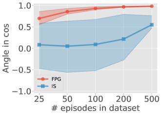
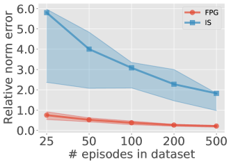
Figure 1: Sample efficiency of FPG on off-policy data. The off-policy PG estimation accuracy is evaluated using two metrics: $\cos\angle(\widehat{\nabla_{\theta}v_{\theta}},\nabla_{\theta}v_{\theta})$ and the relative error norm $\frac{\|\widehat{\nabla_{\theta}v_{\theta}}-\nabla_{\theta}v_{\theta}\|}{\|\nabla_{\theta}v_{\theta}\|}$.

The effect of distributional mismatch

Next we investigate the effect of distribution shift on off-policy PG estimation. We consider $5$ choices of behavior policies: the target policy, the $\varepsilon$-greedy policies of the target policy, with $\varepsilon=0.1$, $0.3$, $0.5$ and $0.7$. We generate a dataset containing $200$ episodes with each of these behavior policies, run FPG and IS, and evaluate their estimation errors. Figure 2 shows that larger distribution mismatch leads to larger estimation error in both methods. However, when compared to IS, FPG is significantly more robust to off-policy distribution shift. The accuracy of FPG only degrades slightly with larger distribution mismatch, while IS suffers from exponentially blowing-up error and stops generating reasonable estimates.

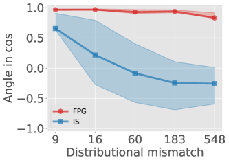
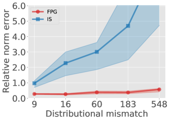
Figure 2: Tolerance to off-policy distribution shift. The distributional mismatch is measured by $\hbox{cond}(\bar{\Sigma}^{\frac{1}{2}}\Sigma^{-1}\bar{\Sigma}^{\frac{1}{2}})$, where $\Sigma$ is the data covariance and $\bar{\Sigma}$ is the target policy’s occupancy measure.

FPG for policy optimization

We further showcase FPG’s applicability to policy optimization. In particular, we test FPG as a gradient estimation module in policy gradient optimization methods. We conduct an experiment using FPG in on-policy REINFORCE and compare it with the vanilla REINFORCE and SVRPG [17]. All methods are configured to sample $100$ on-policy episodes per iteration. When implementing the FPG-REINFORCE, we take advantage of FPG’s off-policy capability and use data from the recent $5$ iterations to improve the gradient estimation accuracy. Figure 3 shows that such design indeed allows FPG-REINFORCE to converge significantly faster than the two baselines.

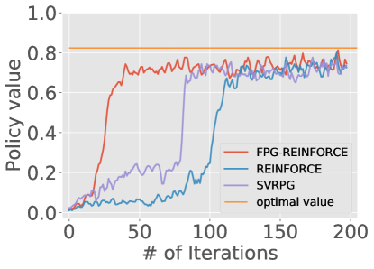
Figure 3: FPG for policy optimization. FPG is used as a module for PG estimates in REINFORCE, compared with other baselines.

Next we test the use of FPG for offline policy optimization. Let the target policy be the optimal policy of the problem, and let the behavior policy be a $0.3$-greedy variant of the target policy. We generate a dataset consisting of $K=500$ episodes by simulating the behavior policy. For PG estimation, we only use the offline dataset and do not sample for fresh data. Thus, we replace the online policy gradient estimator in REINFORCE with an off-policy one using FPG, and for comparison we also test REINFORCE with an IS estimator. Figure 4 shows that FPG-REINFORCE converges reasonably fast and approaches the optimal value. However, IS-REINFORCE appears to converge to a highly biased solution, due to that all PGs are estimated using the same small batch dataset and suffer from bias due to distribution shift.

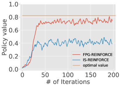
Figure 4: FPG for offline policy optimization. FPG is compared with IS as the PG estimator module in offline REINFORCE.

FPG with deep neural network policy parameterization

Further, we evaluate the efficiency of FPG when using a deep policy network for policy learning in the CliffWalking environment, where $H=100$. Specifically, the environment is modified by adding artificial randomness for stochastic transitions, that is, at each transition, a random action is taken with probability $0.1$. The policy is parameterized with a neural network with one ReLU hidden layer and a softmax layer.

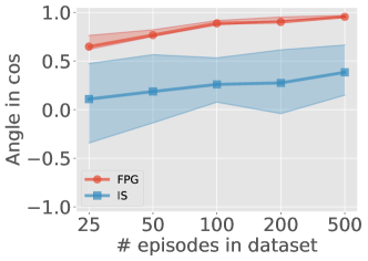
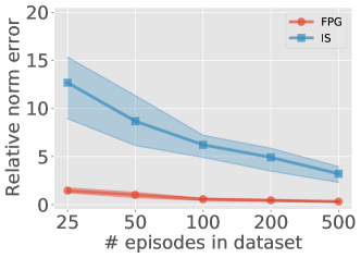
Figure 5: Sample efficiency of FPG with deep policy networks on off-policy data. The off-policy PG estimation accuracy is evaluated using two metrics: $\cos\angle(\widehat{\nabla v_{\theta}},\nabla v_{\theta})$ and the relative error norm $\frac{\|\widehat{\nabla v_{\theta}}-\nabla v_{\theta}\|}{\|\nabla v_{\theta}\|}$.

As before, we test the performance of FPG against the size of off-policy data and the degree of distribution shift, using the same cosine and relative norm error metrics. We test FPG varying the size of the dataset. Figure 5 shows that FPG still gives accurate estimates with moderate variance, in contrast to IS’s inaccuracy and high variance. Both methods become more accurate asymptotically as the dataset size increases.

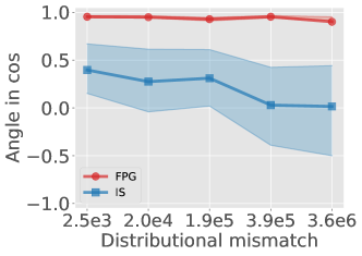
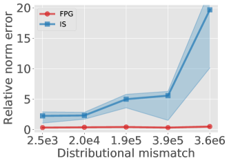
Figure 6: Tolerance to off-policy distribution shift with deep policy networks. The distributional mismatch is measured by $\hbox{cond}(\Sigma^{1/2}\overline{\Sigma}^{-1}\Sigma^{1/2})$, where $\overline{\Sigma}$ is the data covariance and $\Sigma$ is the target policy’s occupancy measure.

We also test FPG on datasets with different amount of mismatch from the target policy. Figure 6 shows that FPG’s estimation error is much lower and less affected by enlarging distributional mismatch than IS’s. The distribution mismatch is large in the CliffWalking experiments because some state-action pairs are almost never visited by the target policy and seldom visited by the behavior policy. Such state-action pairs cause $\Sigma^{1/2}\overline{\Sigma}^{-1}\Sigma^{1/2}$ to be nearly singular, but they are irrelevant to our estimation. The general trends in these CliffWalking experiments with deep neural network policy are consistent with our theoretical results and FrozenLake experiments.

Bootstrap inference for FPG

Finally we apply bootstrap inference to construct confidence regions of FPG estimates by subsampling episodes and estimating the bootstrapped probability distribution. We plot contours of bootstrapped confidence regions via quantile KDE. Figure 7 visualizes the bootstrapped confidence regions in 2D, compared with the confidence region for IS and the ground-truth confidence set. Across all experiments, we observe that the contours of bootstrapping FPG are much smaller and more accurate than the ones of bootstrapping IS. As the $K$ increases, the bootstrapped confidence regions become more concentrated, confirming our theoretical results.

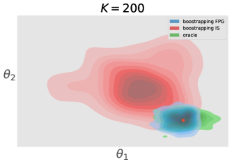
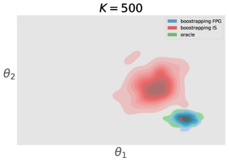
Figure 7: Bootstrapped confidence region for FPG estimator, with sample size $K=200,500$. The red dot marks the true gradient. Blue and red areas are confidence sets obtained by bootstrapping FPG and IS respectively. The green oracle gives the empirical confidence region for FPG estimates.

8 Conclusion

We propose double Fitted Policy Gradient iteration (FPG) for off-policy PG estimation. FPG theoretically achieves near-optimal rate that matches the Cramar-Rao lower bound and empirically outperforms classic methods on a variety of tasks. Future work includes extension to non-linear function approximation and evaluation on more complex domains.

Appendix A Technical Lemmas

Let $U_{h}^{\theta}=\mathcal{P}_{\theta,h}\left(\nabla_{\theta}\log\Pi_{\theta,h+1}\right)Q_{h+1}^{\theta},\ \widehat{U}_{h}^{\theta}=\widehat{\mathcal{P}}_{\theta,h}\left(\nabla_{\theta}\log\Pi_{\theta,h+1}\right)Q_{h+1}^{\theta},\ \tilde{U}_{h}^{\theta}=\widehat{\mathcal{P}}_{\theta,h}\left(\nabla_{\theta}\log\Pi_{\theta,h+1}\right)\widehat{Q}_{h+1}^{\theta}$,

Lemma A.1.

We have

$$Q_{h}^{\theta} =\sum_{h^{\prime}=h}^{H}\left(\prod_{h^{\prime\prime}=h}^{h^{\prime}-1}\mathcal{P}_{\theta,h^{\prime\prime}}\right)r_{h^{\prime}},\quad\widehat{Q_{h}^{\theta}}=\sum_{h^{\prime}=h}^{H}\left(\prod_{h^{\prime\prime}=h}^{h^{\prime}-1}\widehat{\mathcal{P}}_{\theta,h^{\prime\prime}}\right)\widehat{r}_{h^{\prime}},$$

$$\nabla_{\theta}Q_{h}^{\theta} =\sum_{h^{\prime}=h}^{H}\left(\prod_{h^{\prime\prime}=h}^{h^{\prime}-1}\mathcal{P}_{\theta,h^{\prime\prime}}\right)U_{h^{\prime}}^{\theta},\quad\widehat{\nabla_{\theta}Q_{h}^{\theta}}=\sum_{h^{\prime}=h}^{H}\left(\prod_{h^{\prime\prime}=h}^{h^{\prime}-1}\widehat{\mathcal{P}}_{\theta,h^{\prime\prime}}\right)\tilde{U}_{h^{\prime}}^{\theta}.$$

Proof.

By Bellman’s equation, we have $Q_{h}^{\theta}=r_{h}+\mathcal{P}_{\theta,h}Q_{h+1}^{\theta}$. Therefore, by induction and use the fact that $Q_{H+1}^{\theta}=0$, we have proved the first equation. By the policy gradient Bellman’s equation, we have

$$\nabla_{\theta}Q_{h}^{\theta}(s,a) =\mathbb{E}^{\pi_{\theta}}\left[\left(\nabla_{\theta}\log\pi_{\theta,h+1}(a^{\prime}|s^{\prime})\right)Q_{h+1}^{\theta}(s^{\prime},a^{\prime})|s,a,h\right]+\mathbb{E}^{\pi_{\theta}}\left[\nabla_{\theta}Q_{h+1}^{\theta}(s^{\prime},a^{\prime})|s,a,h\right],$$

i.e., $\nabla_{\theta}Q_{h}^{\theta}=U_{h}^{\theta}+\mathcal{P}_{\theta,h}\nabla_{\theta}Q_{h+1}^{\theta}$. By induction, we have proved the third equation. The expressions of $\widehat{Q}_{h}^{\theta}$ and $\widehat{\nabla_{\theta}Q_{h}^{\theta}}$ can be derived directly from their definitions and induction. ∎

The decomposition leads to the following boundedness result:

Lemma A.2.

We have $|Q_{h}^{\theta}(s,a)|\leq H-h+1,\ \|\nabla_{\theta}Q_{h}^{\theta}(s,a)\|_{\infty}\leq G(H-h)^{2},\ \forall s\in\mathcal{S},a\in\mathcal{A},h\in[H].$

Now we consider the decomposition of $Q_{h}^{\theta}-\widehat{Q}_{h}^{\theta}$:

Lemma A.3.

We have

$$Q_{h}^{\theta}-\widehat{Q}_{h}^{\theta}=\sum_{h^{\prime}=h}^{H}\left(\prod_{h^{\prime\prime}=h}^{h^{\prime}-1}\widehat{\mathcal{P}}_{\theta,h^{\prime\prime}}\right)\left(Q_{h^{\prime}}^{\theta}-\widehat{r}_{h^{\prime}}-\widehat{\mathcal{P}}_{\theta,h^{\prime}}Q_{h^{\prime}+1}^{\theta}\right),\quad\forall h\in[H].$$

Proof.

Simply note that

$$Q_{h}^{\theta}-\widehat{Q}_{h}^{\theta} =\sum_{h^{\prime}=h}^{H}\left(\prod_{h^{\prime\prime}=h}^{h^{\prime}-1}\mathcal{P}_{\theta,h^{\prime\prime}}\right)r_{h^{\prime}}-\sum_{h^{\prime}=h}^{H}\left(\prod_{h^{\prime\prime}=h}^{h^{\prime}-1}\widehat{\mathcal{P}}_{\theta,h^{\prime\prime}}\right)\widehat{r}_{h^{\prime}}$$

$$=\sum_{h^{\prime}=h}^{H}\left(\left(\prod_{h^{\prime\prime}=h}^{h^{\prime}-1}\mathcal{P}_{\theta,h^{\prime\prime}}\right)-\left(\prod_{h^{\prime\prime}=h}^{h^{\prime}-1}\widehat{\mathcal{P}}_{\theta,h^{\prime\prime}}\right)\right)r_{h^{\prime}}+\sum_{h^{\prime}=h}^{H}\left(\prod_{h^{\prime\prime}=h}^{h^{\prime}-1}\widehat{\mathcal{P}}_{\theta,h^{\prime\prime}}\right)\left(r_{h^{\prime}}-\widehat{r}_{h^{\prime}}\right)$$

$$=\sum_{h^{\prime}=h}^{H}\sum_{h^{\prime\prime}=h}^{h^{\prime}-1}\left(\prod_{h^{\prime\prime\prime}=h}^{h^{\prime\prime}-1}\widehat{\mathcal{P}}_{\theta,h^{\prime\prime\prime}}\right)\left(\mathcal{P}_{\theta,h^{\prime\prime}}-\widehat{\mathcal{P}}_{\theta,h^{\prime\prime}}\right)\left(\prod_{h^{\prime\prime\prime}=h^{\prime\prime}+1}^{h^{\prime}-1}\mathcal{P}_{\theta,h^{\prime\prime\prime}}\right)r_{h^{\prime}}+\sum_{h^{\prime}=h}^{H}\left(\prod_{h^{\prime\prime}=h}^{h^{\prime}-1}\widehat{\mathcal{P}}_{\theta,h^{\prime\prime}}\right)\left(r_{h^{\prime}}-\widehat{r}_{h^{\prime}}\right)$$

$$=\sum_{h^{\prime\prime}=h}^{H}\left(\prod_{h^{\prime\prime\prime}=h}^{h^{\prime\prime}-1}\widehat{\mathcal{P}}_{\theta,h^{\prime\prime\prime}}\right)\left(\mathcal{P}_{\theta,h^{\prime\prime}}-\widehat{\mathcal{P}}_{\theta,h^{\prime\prime}}\right)\sum_{h^{\prime}=h^{\prime\prime}+1}^{H}\left(\prod_{h^{\prime\prime\prime}=h^{\prime\prime}+1}^{h^{\prime}-1}\mathcal{P}_{\theta,h^{\prime\prime\prime}}\right)r_{h^{\prime}}+\sum_{h^{\prime}=h}^{H}\left(\prod_{h^{\prime\prime}=h}^{h^{\prime}-1}\widehat{\mathcal{P}}_{\theta,h^{\prime\prime}}\right)\left(r_{h^{\prime}}-\widehat{r}_{h^{\prime}}\right)$$

$$=\sum_{h^{\prime}=h}^{H}\left(\prod_{h^{\prime\prime}=h}^{h^{\prime}-1}\widehat{\mathcal{P}}_{\theta,h^{\prime\prime}}\right)\left(\mathcal{P}_{\theta,h^{\prime}}-\widehat{\mathcal{P}}_{\theta,h^{\prime}}\right)Q^{\theta}_{h^{\prime}+1}+\sum_{h^{\prime}=h}^{H}\left(\prod_{h^{\prime\prime}=h}^{h^{\prime}-1}\widehat{\mathcal{P}}_{\theta,h^{\prime\prime}}\right)\left(r_{h^{\prime}}-\widehat{r}_{h^{\prime}}\right)$$

$$=\sum_{h^{\prime}=h}^{H}\left(\prod_{h^{\prime\prime}=h}^{h^{\prime}-1}\widehat{\mathcal{P}}_{\theta,h^{\prime\prime}}\right)\left(Q_{h^{\prime}}^{\theta}-\widehat{r}_{h^{\prime}}-\widehat{\mathcal{P}}_{\theta,h^{\prime}}Q_{h^{\prime}+1}^{\theta}\right),$$

which is the desired result. ∎

The following lemma provides an upper bound of matrix production, which will be used when bounding the higher order terms of the finite sample bound.

Lemma A.4.

For any series of matrices $A_{1},A_{2},\ldots,A_{n}$ and $\Delta A_{1},\Delta A_{2},\ldots\Delta A_{n}$, we have

$$\left\|\prod_{i=1}^{n}(A_{i}+\Delta A_{i})-\prod_{i=1}^{n}A_{i}\right\|\leq\prod_{i=1}^{n}\left(\|A_{i}\|+\|\Delta A_{i}\|\right)-\prod_{i=1}^{n}\|A_{i}\|.$$

Proof.

We have

$$\left\|\prod_{i=1}^{n}(A_{i}+\Delta A_{i})-\prod_{i=1}^{n}A_{i}\right\| =\left\|\sum_{\delta\in\{0,1\}^{n}\setminus\{(1,1,\ldots,1)\}}\prod_{i=1}^{n}A_{i}^{\delta_{i}}(\Delta A_{i})^{1-\delta_{i}}\right\|\leq\sum_{\delta\in\{0,1\}^{n}\setminus\{(1,1,\ldots,1)\}}\prod_{i=1}^{n}\|A_{i}\|^{\delta_{i}}\|\Delta A_{i}\|^{1-\delta_{i}}$$

$$=\prod_{i=1}^{n}\left(\|A_{i}\|+\|\Delta A_{i}\|\right)-\prod_{i=1}^{n}\|A_{i}\|.$$

∎

When $\mathcal{F}$ is the class of the linear functions, there exists matrix $M_{\theta,h}$ such that the transition probability satisfies

$$\mathbb{E}^{\pi_{\theta}}\left[\phi(s^{\prime},a^{\prime})^{\top}|s,a,h\right]=\phi(s,a)^{\top}M_{\theta,h}.$$

The following lemma gives an upper bound on the 2-norm of $M_{\theta,h}$ and its derivatives.

Lemma A.5.

We have $\left\|\Sigma_{\theta,h}^{\frac{1}{2}}M_{\theta,h}\Sigma_{\theta,h+1}^{-\frac{1}{2}}\right\|\leq 1$ and $\left\|\Sigma_{\theta,h}^{\frac{1}{2}}\left(\nabla_{\theta}^{j}M_{\theta,h}\right)\Sigma_{\theta,h+1}^{-\frac{1}{2}}\right\|\leq G,\ \forall j\in[m],h\in[H]$.

Proof.

Note that for any $f:\mathcal{S}\times\mathcal{A}\rightarrow\mathbb{R},\ f(s,a):=\mu^{\top}\phi(s,a)$, we have

$$\mathbb{E}^{\pi_{\theta}}\left[f^{2}(s_{h+1},a_{h+1})|s_{1}\sim\xi\right] =\mathbb{E}^{\pi_{\theta}}\left[\mathbb{E}^{\pi_{\theta}}\left[f^{2}(s_{h+1},a_{h+1})|s_{h},a_{h}\right]|s_{1}\sim\xi\right]$$

$$\geq\mathbb{E}^{\pi_{\theta}}[\mathbb{E}^{\pi_{\theta}}[f(s_{h+1},a_{h+1})|s_{h},a_{h}]^{2}|s_{1}\sim\xi]$$

The LHS satisfies

$$\mathbb{E}^{\pi_{\theta}}[f^{2}(s_{h+1},a_{h+1})|s_{1}\sim\xi] =\mu^{\top}\Sigma_{\theta,h+1}\mu$$

and the RHS satisfies

$$\mathbb{E}^{\pi_{\theta}}[\mathbb{E}^{\pi_{\theta}}[f(s_{h+1},a_{h+1})|s_{h},a_{h}]^{2}|s_{1}\sim\xi]=\mathbb{E}^{\pi_{\theta}}[\mu^{\top}M_{\theta,h}^{\top}\phi(s_{h},a_{h})\phi(s_{h},a_{h})^{\top}M_{\theta,h}\mu|s_{1}\sim\xi]=\mu^{\top}M_{\theta,h}^{\top}\Sigma_{\theta,h}M_{\theta,h}\mu$$

Therefore, we have $\mu^{\top}\Sigma_{\theta,h+1}\mu\geq\mu^{\top}M_{\theta,h}^{\top}\Sigma_{\theta,h}M_{\theta,h}\mu,\ \forall\mu$, which implies $\|\Sigma_{\theta,h}^{\frac{1}{2}}M_{\theta,h}\Sigma_{\theta,h+1}^{-\frac{1}{2}}\|\leq 1$. Similarly, let $g:\mathcal{S}\times\mathcal{A}\rightarrow\mathbb{R},\ g(s,a):=\left(\nabla_{\theta}^{j}\log\pi_{\theta,h+1}(s,a)\right)\mu^{\top}\phi(s,a)$, we have

$$\mathbb{E}^{\pi_{\theta}}[g^{2}(s_{h+1},a_{h+1})|s_{1}\sim\xi]= \mathbb{E}^{\pi_{\theta}}[\mathbb{E}^{\pi_{\theta}}[g^{2}(s_{h+1},a_{h+1})|s_{h},a_{h}]|s_{1}\sim\xi]$$

$$\geq \mathbb{E}^{\pi_{\theta}}[\mathbb{E}^{\pi_{\theta}}[g(s_{h+1},a_{h+1})|s_{h},a_{h}]^{2}|s_{1}\sim\xi]$$

The LHS satisfies

$$\mathbb{E}^{\pi_{\theta}}[g^{2}(s_{h+1},a_{h+1})|s_{1}\sim\xi] =\mu^{\top}\mathbb{E}^{\pi_{\theta}}\left[\left(\nabla_{\theta}^{j}\log\pi_{\theta,h+1}(a|s)\right)^{2}\phi(s_{h+1},a_{h+1})\phi(s_{h+1},a_{h+1})^{\top}|s_{1}\sim\xi\right]\mu$$

$$\leq G^{2}\mu^{\top}\mathbb{E}^{\pi_{\theta}}\left[\phi(s_{h+1},a_{h+1})\phi(s_{h+1},a_{h+1})^{\top}|s_{1}\sim\xi\right]\mu=G^{2}\mu^{\top}\Sigma_{\theta,h+1}\mu$$

and the RHS satisfies

$$\mathbb{E}^{\pi_{\theta}}[\mathbb{E}^{\pi_{\theta}}[g(s_{h+1},a_{h+1})|s_{h},a_{h}]^{2}|s_{1}\sim\xi]$$

$$= \mathbb{E}^{\pi_{\theta}}[\mu^{\top}\left(\nabla_{\theta}^{j}M_{\theta,h}\right)^{\top}\phi(s_{h},a_{h})\phi(s_{h},a_{h})^{\top}\left(\nabla_{\theta}^{j}M_{\theta,h}\right)\mu|s_{1}\sim\xi]$$

$$= \mu^{\top}\left(\nabla_{\theta}^{j}M_{\theta,h}\right)^{\top}\Sigma_{\theta,h}\left(\nabla_{\theta}^{j}M_{\theta,h}\right)\mu.$$

Therefore, we get $G^{2}\mu^{\top}\Sigma_{\theta,h+1}\mu\geq\mu^{\top}\left(\nabla_{\theta}^{j}M_{\theta,h}\right)^{\top}\Sigma_{\theta,h}\left(\nabla_{\theta}^{j}M_{\theta,h}\right)\mu,\ \forall\mu$, which implies $\left\|\Sigma_{\theta,h}^{\frac{1}{2}}\left(\nabla_{\theta}^{j}M_{\theta}\right)\Sigma_{\theta,h+1}^{-\frac{1}{2}}\right\|\leq G$. ∎

Lemma A.6.

We have with probability at least $1-\delta$,

$$\left\|\Sigma_{h}^{-\frac{1}{2}}\left(\frac{1}{K}\sum_{k=1}^{K}\phi(s_{h}^{(k)},a_{h}^{(k)})\phi(s_{h}^{(k)},a_{h}^{(k)})^{\top}\right)\Sigma^{-\frac{1}{2}}_{h}-I_{d}\right\|\leq\sqrt{\frac{2C_{1}d\log\frac{2dH}{\delta}}{K}}+\frac{2C_{1}d\log\frac{2dH}{\delta}}{3K}.$$

Proof.

Define

$$X^{(k)}_{h}=\Sigma^{-\frac{1}{2}}_{h}\phi\left(s^{(k)}_{h},a^{(k)}_{h}\right)\phi\left(s^{(k)}_{h},a^{(k)}_{h}\right)^{\top}\Sigma_{h}^{-\frac{1}{2}}\in\mathbb{R}^{d\times d}.$$

It’s easy to see that $X^{(1)}_{h},X^{(2)}_{h},\ldots,X^{(K)}_{h}$ are independent and $\mathbb{E}\left[X^{(k)}_{h}\right]=I_{d}$. In the remaining part of the proof, we will apply the matrix Bernstein’s inequality to analyze the concentration of $\frac{1}{K}\sum_{k=1}^{K}X^{(k)}_{h}$. We first consider the matrix-valued variance $\textrm{Var}\left(X^{(k)}_{h}\right)=\mathbb{E}\left[\left(X^{(k)}_{h}-I_{d}\right)^{2}\right]=\mathbb{E}\left[\left(X^{(k)}_{h}\right)^{2}\right]-I_{d}$. For any vector $\mu\in\mathbb{R}^{d}$,

$$\mu^{\top}\mathbb{E}\left[\left(X_{h}^{(k)}\right)^{2}\right]\mu= \mathbb{E}\left[\left\|X_{h}^{(k)}\mu\right\|^{2}\right]=\mathbb{E}\left[\left\|\Sigma^{-\frac{1}{2}}_{h}\phi\left(s^{(k)}_{h},a^{(k)}_{h}\right)\phi\left(s^{(k)}_{h},a^{(k)}_{h}\right)^{\top}\Sigma_{h}^{-\frac{1}{2}}\mu\right\|^{2}\right]$$

$$\leq \mathbb{E}\left[\left\|\Sigma_{h}^{-\frac{1}{2}}\phi\left(s^{(k)}_{h},a^{(k)}_{h}\right)\right\|^{2}\left\|\phi\left(s^{(k)}_{h},a^{(k)}_{h}\right)^{\top}\Sigma_{h}^{-\frac{1}{2}}\mu\right\|^{2}\right]\leq C_{1}d\mathbb{E}\left[\left\|\phi\left(s^{(k)}_{h},a^{(k)}_{h}\right)^{\top}\Sigma_{h}^{-\frac{1}{2}}\mu\right\|^{2}\right]$$

$$= C_{1}d\mu^{\top}\mathbb{E}\left[X_{h}^{(k)}\right]\mu=C_{1}d\|\mu\|^{2},$$

where we used the identity $\left\|\phi\left(s^{(k)}_{h},a^{(k)}_{h}\right)^{\top}\Sigma_{h}^{-\frac{1}{2}}\mu\right\|^{2}=\mu^{\top}X_{h}^{(k)}\mu$ and $\mathbb{E}\left[X_{h}^{(k)}\right]=I_{d}$. We have

$$\textrm{Var}(X_{h}^{(k)})\preceq\mathbb{E}\left[\left(X_{h}^{(k)}\right)^{2}\right]\preceq C_{1}dI_{d}.$$

Additionally,

$$-I_{d}\preceq X_{h}^{(k)}-I_{d}=\Sigma_{h}^{-\frac{1}{2}}\phi\left(s^{(k)}_{h},a^{(k)}_{h}\right)\phi\left(s^{(k)}_{h},a^{(k)}_{h}\right)^{\top}\Sigma_{h}^{-\frac{1}{2}}-I_{d}\preceq C_{1}dI_{d}-I_{d}.$$

Therefore, $\|X_{h}^{(k)}-I_{d}\|\leq C_{1}d$. Since $X^{(1)}_{h},X^{(2)}_{h},\ldots,X^{(K)}_{h}$ are i.i.d., by the matrix-form Bernstein inequality, we have

$$\mathbb{P}\left(\left\|\sum_{k=1}^{K}X_{h}^{(k)}-I_{d}\right\|\geq\varepsilon\right)\leq 2d\cdot\exp\left(-\frac{\varepsilon^{2}/2}{C_{1}dK+C_{1}d\varepsilon/3}\right),\quad\forall\varepsilon>0.$$

With probability at least $1-\delta$,

$$\left\|\frac{1}{K}\sum_{k=1}^{K}\left(X_{h}^{(k)}-I_{d}\right)\right\|\leq\sqrt{\frac{2C_{1}d\log\frac{2d}{\delta}}{K}}+\frac{2C_{1}d\log\frac{2d}{\delta}}{3K},$$

Taking a union bound over $h\in[H]$, we derive the desired result. ∎

Let $\Delta\Sigma_{h}^{-1}=\widehat{\Sigma}_{h}^{-1}-\Sigma_{h}$,

Lemma A.7.

If $\left\|\Sigma_{h}^{-\frac{1}{2}}\widehat{\Sigma}_{h}\Sigma_{h}^{-\frac{1}{2}}-I_{d}\right\|\leq\frac{1}{2}$, then $\left\|\Sigma_{h}^{\frac{1}{2}}\left(\Delta\Sigma_{h}^{-1}\right)\Sigma_{h}^{\frac{1}{2}}\right\|\leq 2\left\|\Sigma_{h}^{-\frac{1}{2}}\widehat{\Sigma}_{h}\Sigma_{h}^{-\frac{1}{2}}-I_{d}\right\|$.

Proof.

Note that

$$\left\|\Sigma_{h}^{\frac{1}{2}}\left(\Delta\Sigma_{h}^{-1}\right)\Sigma_{h}^{\frac{1}{2}}\right\|=\left\|\Sigma_{h}^{\frac{1}{2}}\left(\widehat{\Sigma}_{h}^{-1}-\Sigma_{h}^{-1}\right)\Sigma_{h}^{\frac{1}{2}}\right\|\leq\left\|\Sigma_{h}^{\frac{1}{2}}\widehat{\Sigma}_{h}^{-1}\Sigma_{h}^{\frac{1}{2}}\right\|\left\|\Sigma_{h}^{-\frac{1}{2}}\widehat{\Sigma}_{h}\Sigma_{h}^{-\frac{1}{2}}-I_{d}\right\|.$$ (7)

Because we have $\left\|\Sigma_{h}^{-\frac{1}{2}}\widehat{\Sigma}_{h}\Sigma_{h}^{-\frac{1}{2}}-I_{d}\right\|\leq\frac{1}{2}$, we get $\sigma_{\textrm{min}}\left(\Sigma_{h}^{-\frac{1}{2}}\widehat{\Sigma}_{h}\Sigma_{h}^{-\frac{1}{2}}\right)\geq\frac{1}{2}$, which implies $\left\|\Sigma_{h}^{\frac{1}{2}}\widehat{\Sigma}_{h}^{-1}\Sigma_{h}^{\frac{1}{2}}\right\|\leq 2$. Combining this result with (7) finishes the proof. ∎

Let $\Delta Y_{\theta,h}=\frac{1}{K}\sum_{k=1}^{K}\phi\left(s_{h}^{(k)},a_{h}^{(k)}\right)\phi_{\theta,h+1}\left(s_{h+1}^{(k)}\right)^{\top}-\Sigma_{h}M_{\theta,h}$,

Lemma A.8.

With probability at least $1-\delta$, the following inequalities hold simultaneously:

$$\left\|\Sigma_{h}^{-\frac{1}{2}}\left(\Delta Y_{\theta,h}\right)\Sigma_{h+1}^{-\frac{1}{2}}\right\| \leq\left(\kappa_{2}\vee 1\right)\sqrt{\frac{2C_{1}d\log\frac{4dH}{\delta}}{K}}+\frac{4C_{1}d\log\frac{4dH}{\delta}}{3K},$$ (8)

$$\left\|\Sigma_{h}^{-\frac{1}{2}}\left(\nabla_{\theta}^{j}\left(\Delta Y_{\theta,h}\right)\right)\Sigma_{h+1}^{-\frac{1}{2}}\right\| \leq\left(\kappa_{3}\vee 1\right)G\sqrt{\frac{2C_{1}d\log\frac{4mdH}{\delta}}{K}}+\frac{4C_{1}dG\log\frac{4mdH}{\delta}}{3K},\quad\forall j\in[m],$$ (9)

where $\kappa_{2},\kappa_{3}$ are defined in Theorem 6.2.

Proof.

Take

$$Y_{\theta,h}^{(k)}:=\Sigma_{h}^{-\frac{1}{2}}\phi\left(s^{(k)}_{h},a^{(k)}_{h}\right)\phi_{\theta,h+1}\left(s^{(k)}_{h+1}\right)^{\top}\Sigma_{h+1}^{-\frac{1}{2}},\quad\forall k\in[K].$$

Then, $\Sigma_{h}^{-\frac{1}{2}}\left(\Delta Y_{\theta,h}\right)\Sigma_{h+1}^{-\frac{1}{2}}=\frac{1}{K}\sum_{k=1}^{K}\left(Y_{\theta,h}^{(k)}-\Sigma_{h}^{\frac{1}{2}}M_{\theta,h}\Sigma^{-\frac{1}{2}}_{h+1}\right)$. Note that

$$\begin{aligned} \mathbb{E}\left[Y_{\theta,h}^{(k)}\right]=&\mathbb{E}\left[\Sigma_{h}^{-\frac{1}{2}}\phi\left(s^{(k)}_{h},a^{(k)}_{h}\right)\phi_{\theta,h+1}\left(s^{(k)}_{h+1}\right)^{\top}\Sigma_{h+1}^{-\frac{1}{2}}\right]\\ =&\mathbb{E}\left[\Sigma_{h}^{-\frac{1}{2}}\phi\left(s^{(k)}_{h},a^{(k)}_{h}\right)\mathbb{E}^{\pi_{\theta}}\left[\phi\left(s^{\prime},a^{\prime}\right)^{\top}|s^{(k)}_{h},a^{(k)}_{h},h\right]\Sigma_{h+1}^{-\frac{1}{2}}\right]\\ =&\mathbb{E}\left[\Sigma_{h}^{-\frac{1}{2}}\phi\left(s^{(k)}_{h},a^{(k)}_{h}\right)\phi\left(s^{(k)}_{h},a^{(k)}_{h}\right)^{\top}M_{\theta,h}\Sigma_{h+1}^{-\frac{1}{2}}\right]=\Sigma_{h}^{\frac{1}{2}}M_{\theta,h}\Sigma_{h+1}^{-\frac{1}{2}},\end{aligned}$$ (10)

To this end, $\Sigma_{h}^{-\frac{1}{2}}\left(\Delta Y_{\theta,h}\right)\Sigma_{h+1}^{-\frac{1}{2}}=\frac{1}{K}\sum_{k=1}^{K}\left(Y_{\theta,h}^{(k)}-\mathbb{E}\left[Y_{\theta,h}^{(k)}\right]\right)$. Since the trajectories are i.i.d., we use the matrix-form Bernstein inequality to estimate $\left\|\Sigma_{h}^{-\frac{1}{2}}(\Delta Y_{\theta,h})\Sigma_{h+1}^{-\frac{1}{2}}\right\|$. For any $\mu\in\mathbb{R}^{d}$, we have

$$\mu^{\top}\mathbb{E}\left[Y_{\theta,h}^{(k)}\left(Y_{\theta,h}^{(k)}\right)^{\top}\right]\mu= \mathbb{E}\left[\left\|\left(Y_{\theta,h}^{(k)}\right)^{\top}\mu\right\|^{2}\right]=\mathbb{E}\left[\left\|\Sigma_{h+1}^{-\frac{1}{2}}\phi_{\theta,h+1}\left(s_{h+1}^{(k)}\right)\phi\left(s_{h}^{(k)},a_{h}^{(k)}\right)^{\top}\Sigma_{h}^{-\frac{1}{2}}\mu\right\|^{2}\right]$$

$$\leq \mathbb{E}\left[\left\|\Sigma_{h+1}^{-\frac{1}{2}}\phi_{\theta,h+1}\left(s_{h+1}^{(k)}\right)\right\|^{2}\left\|\phi\left(s_{h}^{(k)},a_{h}^{(k)}\right)^{\top}\Sigma_{h}^{-\frac{1}{2}}\mu\right\|^{2}\right].$$

Parallel to the proof of Lemma A.6, it holds that $\left\|\Sigma_{h+1}^{-\frac{1}{2}}\phi_{\theta,h+1}\left(s_{h+1}^{(k)}\right)\right\|^{2}\leq C_{1}d$. Therefore,

$$\mu^{\top}\mathbb{E}\left[Y_{\theta,h}^{(k)}\left(Y_{\theta,h}^{(k)}\right)^{\top}\right]\mu \leq\mathbb{E}\left[C_{1}d\left\|\phi\left(s_{h}^{(k)},a_{h}^{(k)}\right)^{\top}\Sigma_{h}^{-\frac{1}{2}}\mu\right\|^{2}\right]$$

$$=C_{1}d\mu^{\top}\Sigma_{h}^{-\frac{1}{2}}\mathbb{E}\left[\phi\left(s_{h}^{(k)},a_{h}^{(k)}\right)\phi\left(s_{h}^{(k)},a_{h}^{(k)}\right)^{\top}\right]\Sigma_{h}^{-\frac{1}{2}}\mu$$

$$=C_{1}d\|\mu\|^{2},$$

where we have used the fact $\Sigma_{h}=\mathbb{E}\left[\phi\left(s_{h}^{(k)},a_{h}^{(k)}\right)\phi\left(s_{h}^{(k)},a_{h}^{(k)}\right)^{\top}\right]$. It follows that

$$\textrm{Var}_{1}\left(Y_{\theta,h}^{(k)}\right):= \mathbb{E}\left[\left(Y_{\theta,h}^{(k)}-\mathbb{E}\left[Y_{\theta,h}^{(k)}\right]\right)\left(Y_{\theta,h}^{(k)}-\mathbb{E}\left[Y_{\theta,h}^{(k)}\right]\right)^{\top}\right]\preceq\mathbb{E}\left[Y_{\theta,h}^{(k)}\left(Y_{\theta,h}^{(k)}\right)^{\top}\right]\preceq C_{1}dI_{d}.$$

Analogously,

$$\textrm{Var}_{2}\left(Y_{\theta,h}^{(k)}\right):= \mathbb{E}\left[\left(Y_{\theta,h}^{(k)}-\mathbb{E}\left[Y_{\theta,h}^{(k)}\right]\right)^{\top}\left(Y_{\theta,h}^{(k)}-\mathbb{E}\left[Y_{\theta,h}^{(k)}\right]\right)\right]\preceq\mathbb{E}\left[\left(Y_{\theta,h}^{(k)}\right)^{\top}Y_{\theta,h}^{(k)}\right]$$

$$\preceq C_{1}d\Sigma_{h+1}^{-\frac{1}{2}}\mathbb{E}\left[\phi_{\theta,h+1}\left(s_{h+1}^{(k)}\right)\phi_{\theta,h+1}\left(s_{h+1}^{(k)}\right)^{\top}\right]\Sigma_{h+1}^{-\frac{1}{2}}.$$

Therefore, $\max\left\{\left\|\textrm{Var}_{1}\left(Y_{\theta,h}^{(k)}\right)\right\|,\left\|\textrm{Var}_{2}\left(Y_{\theta,h}^{(k)}\right)\right\|\right\}\leq C_{1}d\left(\kappa_{2}^{2}\vee 1\right)$. It also holds that $\|Y_{\theta,h}^{(k)}\|\leq C_{1}d$. Hence,

$$\left\|Y_{\theta,h}^{(k)}-\Sigma_{h}^{\frac{1}{2}}M_{\theta,h}\Sigma_{h+1}^{-\frac{1}{2}}\right\|\leq 2C_{1}d.$$

Applying Matrix Bernstein’s inequality, we derive for any $\varepsilon>0$,

$$\mathbb{P}\left(\left\|\sum_{k=1}^{K}\left(Y_{\theta,h}^{(k)}-\Sigma_{h}^{\frac{1}{2}}M_{\theta,h}\Sigma_{h+1}^{-\frac{1}{2}}\right)\right\|>\varepsilon\right)\leq 2d\exp\left(-\frac{\varepsilon^{2}/2}{C_{1}dK\left(\kappa_{2}^{2}\vee 1\right)+2C_{1}d\varepsilon/3}\right),$$

which implies (8) holds with probability $1-\frac{\delta}{2}$. For (9), notice that for any $j\in[m]$, we have $\Sigma_{h}^{-\frac{1}{2}}(\nabla_{\theta}^{j}(\Delta Y_{\theta,h}))\Sigma_{h+1}^{-\frac{1}{2}}=\frac{1}{K}\sum_{k=1}^{K}\left(\nabla_{\theta}^{j}Y_{\theta,h}^{(k)}-\mathbb{E}\left[\nabla_{\theta}^{j}Y_{\theta,h}^{(k)}\right]\right)$, and $\nabla_{\theta}^{j}Y_{\theta,h}^{(k)}=\Sigma_{h}^{-\frac{1}{2}}\phi\left(s_{h}^{(k)},a_{h}^{(k)}\right)\left(\nabla_{\theta}^{j}\phi_{\theta,h+1}\left(s_{h+1}^{(k)}\right)\right)^{\top}\Sigma_{h+1}^{-\frac{1}{2}}$. For any $\mu\in\mathbb{R}^{d}$, we have

$$\mu^{\top}\mathbb{E}\left[\left(\nabla_{\theta}^{j}Y_{\theta,h}^{(k)}\right)\left(\nabla_{\theta}^{j}Y_{\theta,h}^{(k)}\right)^{\top}\right]\mu= \mathbb{E}\left[\left\|\Sigma_{h+1}^{-\frac{1}{2}}\left(\nabla_{\theta}^{j}\phi_{\theta,h+1}\left(s_{h+1}^{(k)}\right)\right)\phi\left(s_{h}^{(k)},a_{h}^{(k)}\right)^{\top}\Sigma_{h}^{-\frac{1}{2}}\mu\right\|^{2}\right]$$

$$\leq \mathbb{E}\left[\left\|\Sigma_{h+1}^{-\frac{1}{2}}\nabla_{\theta}^{j}\phi_{\theta,h+1}\left(s_{h+1}^{(k)}\right)\right\|^{2}\left\|\phi\left(s_{h}^{(k)},a_{h}^{(k)}\right)^{\top}\Sigma_{h}^{-\frac{1}{2}}\mu\right\|^{2}\right].$$

Since we have

$$\left(\nabla_{\theta}^{j}\phi_{\theta,h+1}\left(s_{h+1}^{(k)}\right)\right)^{\top}\Sigma_{h+1}^{-1}\nabla_{\theta}^{j}\phi_{\theta,h+1}\left(s_{h+1}^{(k)}\right)$$

$$= \int_{\mathcal{A}\times\mathcal{A}}\pi_{\theta,h+1}\left(a\left|s_{h+1}^{(k)}\right.\right)\pi_{\theta,h+1}\left(a^{\prime}\left|s_{h+1}^{(k)}\right.\right)\left(\nabla_{\theta}^{j}\log\pi_{\theta,h+1}\left(a\left|s_{h+1}^{(k)}\right.\right)\right)\left(\nabla_{\theta}^{j}\log\pi_{\theta,h+1}\left(a^{\prime}\left|s_{h+1}^{(k)}\right.\right)\right)$$

$$\cdot\phi\left(s_{h+1}^{(k)},a\right)^{\top}\Sigma_{h+1}^{-1}\phi\left(s_{h+1}^{(k)},a^{\prime}\right)\mathrm{d}a\mathrm{d}a^{\prime}$$

$$\leq G^{2}\int_{\mathcal{A}\times\mathcal{A}}\pi_{\theta,h+1}\left(a|s_{h+1}^{(k)}\right)\pi_{\theta,h+1}\left(a^{\prime}|s_{h+1}^{(k)}\right)\left\|\Sigma_{h+1}^{-\frac{1}{2}}\phi\left(s_{h+1}^{(k)},a\right)\right\|\left\|\Sigma_{h+1}^{-\frac{1}{2}}\phi\left(s_{h+1}^{(k)},a^{\prime}\right)\right\|\mathrm{d}a\mathrm{d}a^{\prime}\leq G^{2}C_{1}d,$$

which implies

$$\mu^{\top}\mathbb{E}\left[\left(\nabla_{\theta}^{j}Y_{\theta,h}^{(k)}\right)\left(\nabla_{\theta}^{j}Y_{\theta,h}^{(k)}\right)^{\top}\right]\mu\leq G^{2}C_{1}d\mathbb{E}\left[\left\|\phi\left(s_{h}^{(k)},a_{h}^{(k)}\right)^{\top}\Sigma_{h}^{-\frac{1}{2}}\mu\right\|^{2}\right]=G^{2}C_{1}d\|\mu\|^{2}.$$

Therefore,

$$\textrm{Var}_{1}\left(\nabla_{\theta}^{j}Y_{\theta,h}^{(k)}\right):= \mathbb{E}\left[\left(\nabla_{\theta}^{j}Y_{\theta,h}^{(k)}-\mathbb{E}\left[\nabla_{\theta}^{j}Y_{\theta,h}^{(k)}\right]\right)\left(\nabla_{\theta}^{j}Y_{\theta,h}^{(k)}-\mathbb{E}\left[\nabla_{\theta}^{j}Y_{\theta,h}^{(k)}\right]\right)^{\top}\right]\preceq\mathbb{E}\left[\left(\nabla_{\theta}^{j}Y_{\theta,h}^{(k)}\right)\left(\nabla_{\theta}^{j}Y_{\theta,h}^{(k)}\right)^{\top}\right]\preceq G^{2}C_{1}dI_{d}.$$

Meanwhile, we have

$$\textrm{Var}_{2}\left(\nabla_{\theta}^{j}Y_{\theta,h}^{(k)}\right)\preceq\mathbb{E}\left[\left(\nabla_{\theta}^{j}Y_{\theta,h}^{(k)}\right)^{\top}\nabla_{\theta}^{j}Y_{\theta,h}^{(k)}\right]\preceq C_{1}d\Sigma_{h}^{-\frac{1}{2}}\mathbb{E}\left[\left(\nabla_{\theta}^{j}\phi_{\theta,h+1}\left(s_{h+1}^{(k)}\right)\right)\left(\nabla_{\theta}^{j}\phi_{\theta,h+1}\left(s_{h+1}^{(k)}\right)\right)^{\top}\right]\Sigma_{h}^{-\frac{1}{2}}.$$

In conclusion, we get

$$\max\left\{\left\|\textrm{Var}_{1}\left(\nabla_{\theta}^{j}Y_{\theta,h}^{(k)}\right)\right\|,\left\|\textrm{Var}_{2}\left(\nabla_{\theta}^{j}Y_{\theta,h}^{(k)}\right)\right\|\right\}\leq G^{2}C_{1}d\left(\kappa_{3}^{2}\vee 1\right),$$

Note that $\left\|\nabla_{\theta}^{j}Y_{\theta,h}^{(k)}\right\|\leq C_{1}dG$, we know $\left\|\nabla_{\theta}^{j}Y_{\theta,h}^{(k)}-\mathbb{E}\left[\nabla_{\theta}^{j}Y_{\theta,h}^{(k)}\right]\right\|\leq 2C_{1}dG$. By Matrix Bernstein’s inequality, we get for any $\varepsilon>0$,

$$\mathbb{P}\left(\left\|\sum_{k=1}^{K}\left(\nabla_{\theta}^{j}Y_{k,h}^{\theta}-\Sigma_{h}^{\frac{1}{2}}\left(\nabla_{\theta}^{j}M_{\theta,h}\right)\Sigma_{h+1}^{-\frac{1}{2}}\right)\right\|\geq\varepsilon\right)\leq 2d\exp\left(-\frac{\varepsilon^{2}/2}{G^{2}C_{1}dK\left(\kappa_{3}^{2}\vee 1\right)+2C_{1}dG\varepsilon/3}\right),$$

taking a union bound over all $j\in[m]$ and $h\in[H]$ proves that (9) holds with probability $1-\frac{\delta}{2}$. Using a union bound argument again, we know with probability $1-\delta$, (8) and (9) hold simultaneously, which has finished the proof. ∎

Lemma A.9.

For $h\in[H]$, with probability at least $1-\delta$, the following inequalities hold simultaneously:

$$\left\|\Sigma_{h}^{-\frac{1}{2}}\frac{1}{K}\sum_{k=1}^{K}\phi\left(s_{h}^{(k)},a_{h}^{(k)}\right)\varepsilon_{h,k}^{\theta}\right\| \leq\sqrt{d}(H-h+1)\left(\sqrt{\frac{2\log\frac{8dH}{\delta}}{K}}+\frac{2\sqrt{C_{1}d}\log\frac{8dH}{\delta}}{K}+\frac{2C_{1}d\left(\log\frac{8dH}{\delta}\right)^{\frac{3}{2}}}{3K^{\frac{3}{2}}}\right)$$ (11)

$$\left\|\Sigma_{h}^{-\frac{1}{2}}\frac{1}{K}\sum_{k=1}^{K}\phi\left(s_{h}^{(k)},a_{h}^{(k)}\right)\nabla_{\theta}^{j}\varepsilon_{h,k}^{\theta}\right\| \leq 2\sqrt{d}G(H-h)^{2}\left(\sqrt{\frac{2\log\frac{8mdH}{\delta}}{K}}+\frac{2\sqrt{C_{1}d}\log\frac{8mdH}{\delta}}{K}+\frac{2C_{1}d\left(\log\frac{8mdH}{\delta}\right)^{\frac{3}{2}}}{3K^{\frac{3}{2}}}\right),\forall j\in[m].$$ (12)

Proof.

Let $X_{\theta,h}^{(k)}:=\Sigma_{h}^{-\frac{1}{2}}\phi\left(s_{h}^{(k)},a_{h}^{(k)}\right)\varepsilon_{h,k}^{\theta}\in\mathbb{R}^{d}$ and let $\mathcal{F}_{h,k}$ be $\sigma$-algebra generated by the history up to step $h$ at episode $k$, we have $\mathbb{E}\left[\left.X_{\theta,h}^{(k)}\right|\mathcal{F}_{h,k}\right]=0$. We apply matrix-form Freedman’s inequality to analyze the concentration property. Consider conditional variances $\textrm{Var}_{1}\left[\left.X_{\theta,h}^{(k)}\right|\mathcal{F}_{h,k}\right]:=\mathbb{E}\left[\left.X_{\theta,h}^{(k)}\left(X_{\theta,h}^{(k)}\right)^{\top}\right|\mathcal{F}_{h,k}\right]\in\mathbb{R}^{d\times d}$ and $\textrm{Var}_{2}\left[\left.X_{\theta,h}^{(k)}\right|\mathcal{F}_{h,k}\right]:=\mathbb{E}\left[\left(X_{\theta,h}^{(k)}\right)^{\top}X_{\theta,h}^{(k)}|\mathcal{F}_{h,k}\right]\in\mathbb{R}$. It holds that

$$\left\|\textrm{Var}_{1}\left[\left.X_{\theta,h}^{(k)}\right|\mathcal{F}_{h,k}\right]\right\|= \left\|\mathbb{E}\left[\left.X_{\theta,h}^{(k)}\left(X_{\theta,h}^{(k)}\right)^{\top}\right|\mathcal{F}_{h,k}\right]\right\|\leq\mathbb{E}\left[\left.\left\|X_{\theta,h}^{(k)}\left(X_{\theta,h}^{(k)}\right)^{\top}\right\|\right|\mathcal{F}_{h,k}\right]$$

$$= \mathbb{E}\left[\left.\left\|X_{\theta,h}^{(k)}\right\|^{2}\right|\mathcal{F}_{h,k}\right]=\textrm{Var}_{2}\left[\left.X_{\theta,h}^{(k)}\right|\mathcal{F}_{h,k}\right]$$

and

$$\textrm{Var}_{2}\left[\left.X_{\theta,h}^{(k)}\right|\mathcal{F}_{h,k}\right]= \mathbb{E}\left[\left.\left\|X_{\theta,h}^{(k)}\right\|^{2}\right|\mathcal{F}_{h,k}\right]=\phi\left(s_{h}^{(k)},a_{h}^{(k)}\right)^{\top}\Sigma_{h}^{-1}\phi\left(s_{h}^{(k)},a_{h}^{(k)}\right)\textrm{Var}\left[\left.\varepsilon_{h,k}^{\theta}\right|s_{h}^{(k)},a_{h}^{(k)},h\right]$$

$$\leq (H-h+1)^{2}\phi\left(s_{h}^{(k)},a_{h}^{(k)}\right)^{\top}\Sigma_{h}^{-1}\phi\left(s_{h}^{(k)},a_{h}^{(k)}\right),$$

where we have used $\textrm{Var}\left[\left.\varepsilon_{h,k}^{\theta}\right|s_{h}^{(k)},a_{h}^{(k)},h\right]\leq(H-h+1)^{2}$. Note that

$$\sum_{k=1}^{K}\phi\left(s_{h}^{(k)},a_{h}^{(k)}\right)^{\top}\Sigma_{h}^{-1}\phi\left(s_{h}^{(k)},a_{h}^{(k)}\right)= Kd+K\textrm{Tr}\left(\Sigma_{h}^{-\frac{1}{2}}\left(\frac{1}{K}\sum_{k=1}^{K}\phi\left(s_{h}^{(k)},a_{h}^{(k)}\right)\phi\left(s_{h}^{(k)},a_{h}^{(k)}\right)^{\top}\right)\Sigma_{h}^{-\frac{1}{2}}-I_{d}\right)$$

$$\leq Kd+Kd\left\|\Sigma_{h}^{-\frac{1}{2}}\left(\frac{1}{K}\sum_{k=1}^{K}\phi\left(s_{h}^{(k)},a_{h}^{(k)}\right)\phi\left(s_{h}^{(k)},a_{h}^{(k)}\right)^{\top}\right)\Sigma_{h}^{-\frac{1}{2}}-I_{d}\right\|.$$

We take

$$\sigma^{2}:=Kd(H-h+1)^{2}\left(1+\sqrt{\frac{2C_{1}d\log\frac{8dH}{\delta}}{K}}+\frac{2C_{1}d\log\frac{8dH}{\delta}}{3K}\right).$$ (13)

According to Lemma A.6, it holds that

$$\mathbb{P}\left(\left\|\sum_{k=1}^{K}\textrm{Var}_{1}\left[\left.X_{\theta,h}^{(k)}\right|\mathcal{F}_{h,k}\right]\right\|\leq\sum_{k=1}^{K}\textrm{Var}_{2}\left[\left.X_{\theta,h}^{(k)}\right|\mathcal{F}_{h,k}\right]\leq\sigma^{2}\right)\geq 1-\frac{\delta}{4}.$$ (14)

Additionally, we have $\left\|X_{\theta,h}^{(k)}\right\|\leq(H-h+1)\sqrt{C_{1}d}$. The Freedman’s inequality therefore implies that for any $\varepsilon>0$,

$$\begin{aligned} &\mathbb{P}\left(\left|\sum_{k=1}^{K}X_{\theta,h}^{(k)}\right|\geq\varepsilon,\ \max\left\{\left\|\sum_{k=1}^{K}\textrm{Var}_{1}\left[\left.X_{\theta,h}^{(k)}\right|\mathcal{F}_{h,k}\right]\right\|,\sum_{k=1}^{K}\textrm{Var}_{2}\left[\left.X_{\theta,h}^{(k)}\right|\mathcal{F}_{h,k}\right]\right\}\leq\sigma^{2}\right)\leq 2d\exp\left(-\frac{\varepsilon^{2}/2}{\sigma^{2}+(H-h+1)\sqrt{C_{1}d}\varepsilon/3}\right),\end{aligned}$$ (15)

where $\sigma^{2}$ is defined in (13). We take

$$\varepsilon:=\sigma\sqrt{2\log\frac{8d}{\delta}}+\frac{2(H-h+1)\sqrt{C_{1}d}}{3}\log\frac{8d}{\delta}.$$

Then we get

$$\mathbb{P}\left(\left|\sum_{k=1}^{K}X_{\theta,h}^{(k)}\right|\geq\varepsilon,\ \max\left\{\left\|\sum_{k=1}^{K}\textrm{Var}_{1}\left[\left.X_{\theta,h}^{(k)}\right|\mathcal{F}_{h,k}\right]\right\|,\sum_{k=1}^{K}\textrm{Var}_{2}\left[\left.X_{\theta,h}^{(k)}\right|\mathcal{F}_{h,k}\right]\right\}\leq\sigma^{2}\right)\leq\frac{\delta}{4},$$

which implies

$$\mathbb{P}\left(\left|\sum_{k=1}^{K}X_{\theta,h}^{(k)}\right|\geq\varepsilon\right)\leq \mathbb{P}\left(\left|\sum_{k=1}^{K}X_{\theta,h}^{(k)}\right|\geq\varepsilon,\ \max\left\{\left\|\sum_{k=1}^{K}\textrm{Var}_{1}\left[\left.X_{\theta,h}^{(k)}\right|\mathcal{F}_{h,k}\right]\right\|,\sum_{k=1}^{K}\textrm{Var}_{2}\left[\left.X_{\theta,h}^{(k)}\right|\mathcal{F}_{h,k}\right]\right\}\leq\sigma^{2}\right)$$

$$+\mathbb{P}\left(\max\left\{\left\|\sum_{k=1}^{K}\textrm{Var}_{1}\left[\left.X_{\theta,h}^{(k)}\right|\mathcal{F}_{h,k}\right]\right\|,\sum_{k=1}^{K}\textrm{Var}_{2}\left[\left.X_{\theta,h}^{(k)}\right|\mathcal{F}_{h,k}\right]\right\}>\sigma^{2}\right)\leq\frac{\delta}{2}.$$

which, combined with a union bound over $h\in[H]$, has proved (11). We use Freedman’s inequality again to prove (12). For a fixed $j\in[m]$, we have

$$\left\|\textrm{Var}_{1}\left[\left.\nabla_{\theta}^{j}X_{\theta,h}^{(k)}\right|\mathcal{F}_{h,k}\right]\right\|= \left\|\mathbb{E}\left[\left.\left(\nabla_{\theta}^{j}X_{\theta,h}^{(k)}\right)\left(\nabla_{\theta}^{j}X_{\theta,h}^{(k)}\right)^{\top}\right|\mathcal{F}_{h,k}\right]\right\|\leq\mathbb{E}\left[\left.\left\|\left(\nabla_{\theta}^{j}X_{\theta,h}^{(k)}\right)\left(\nabla_{\theta}^{j}X_{\theta,h}^{(k)}\right)^{\top}\right\|\right|\mathcal{F}_{h,k}\right]$$

$$= \mathbb{E}\left[\left.\left\|\nabla_{\theta}^{j}X_{\theta,h}^{(k)}\right\|^{2}\right|\mathcal{F}_{h,k}\right]=\textrm{Var}_{2}\left[\left.\nabla_{\theta}^{j}X_{\theta,h}^{(k)}\right|\mathcal{F}_{h,k}\right]$$

and

$$\textrm{Var}_{2}\left[\left.\nabla_{\theta}^{j}X_{\theta,h}^{(k)}\right|\mathcal{F}_{h,k}\right]= \mathbb{E}\left[\left.\left\|\nabla_{\theta}^{j}X_{\theta,h}^{(k)}\right\|^{2}\right|\mathcal{F}_{h,k}\right]=\phi\left(s_{h}^{(k)},a_{h}^{(k)}\right)^{\top}\Sigma_{h}^{-1}\phi\left(s_{h}^{(k)},a_{h}^{(k)}\right)\textrm{Var}\left[\left.\nabla_{\theta}^{j}\varepsilon_{h,k}^{\theta}\right|s_{h}^{(k)},a_{h}^{(k)}\right]$$

$$\leq 4G^{2}(H-h)^{2}\phi\left(s_{h}^{(k)},a_{h}^{(k)}\right)^{\top}\Sigma_{h}^{-1}\phi\left(s_{h}^{(k)},a_{h}^{(k)}\right),$$

where we have used $\textrm{Var}\left[\left.\nabla_{\theta}^{j}\varepsilon_{h,k}^{\theta}\right|s_{h}^{(k)},a_{h}^{(k)},h\right]\leq 4G^{2}(H-h)^{2}$. Furthermore, notice that $\left\|\nabla_{\theta}^{j}X_{\theta,h}^{(k)}\right\|\leq 2G(H-h)\sqrt{C_{1}d}$, the remaining steps will be exactly the same as those in the proof of (11), combined with a union bound over $j\in[m]$. In this way, we have proved (12). Taking a union bound again finishes the proof. ∎

Appendix B Proofs of Main Theorems

Define $\widehat{\nu}^{\theta}_{h}:=\left(\prod_{h^{\prime}=1}^{h-1}\widehat{M}_{\theta,h^{\prime}}^{\top}\right)\nu_{1}^{\theta}$. We may prove the following decomposition of $\nabla_{\theta}v_{\theta}-\widehat{\nabla_{\theta}v_{\theta}}$:

Lemma B.1.

We have $\nabla_{\theta}v_{\theta}-\widehat{\nabla_{\theta}v_{\theta}}=E_{1}+E_{2}+E_{3}$, where

$$E_{1}= \sum_{h=1}^{H}\nabla_{\theta}\left[\left(\nu^{\theta}_{h}\right)^{\top}\Sigma^{-1}_{h}\frac{1}{K}\sum_{k=1}^{K}\phi\left(s_{h}^{(k)},a_{h}^{(k)}\right)\varepsilon_{h,k}^{\theta}\right]$$

$$E_{2}= \sum_{h=1}^{H}\nabla_{\theta}\left[\left(\left(\widehat{\nu}^{\theta}_{h}\right)^{\top}\widehat{\Sigma}_{h}^{-1}-\left(\nu^{\theta}_{h}\right)^{\top}\Sigma_{h}^{-1}\right)\frac{1}{K}\sum_{k=1}^{K}\phi\left(s_{h}^{(k)},a_{h}^{(k)}\right)\varepsilon_{h,k}^{\theta}\right]$$

$$E_{3}= \frac{\lambda}{K}\sum_{h=1}^{H}\nabla_{\theta}\left[\left(\widehat{\nu}^{\theta}_{h}\right)^{\top}\widehat{\Sigma}_{h}^{-1}w_{h}^{\theta}\right].$$

The proof of Lemma B.1 is deferred to appendix C. Based on this observation, here we show the proofs of our main theorems.

B.1 Proof of Theorem 6.2

Proof.

We use Lemma B.1 to decompose $\langle\nabla_{\theta}v_{\theta}-\widehat{\nabla_{\theta}v_{\theta}},t\rangle=\langle E_{1},t\rangle+\langle E_{2},t\rangle+\langle E_{3},t\rangle$. To bound each term individually, we introduce the following lemmas, whose proofs are deferred to appendix C.

Lemma B.2.

For any $t\in\mathbb{R}^{m}$, with probability $1-\delta$, we have

$$|\langle E_{1},t\rangle|\leq\sqrt{\frac{2t^{\top}\Lambda_{\theta}t\log(2/\delta)}{K}}+\frac{2\log(2/\delta)\sqrt{C_{1}md}\|t\|B}{3K}.$$

where $B=\sum_{h=1}^{H}(H-h+1)\max_{j\in[m]}\sqrt{\left(\nabla^{j}_{\theta}\nu^{\theta}_{h}\right)^{\top}\Sigma_{h}^{-1}\nabla^{j}_{\theta}\nu^{\theta}_{h}}+2G\sum_{h=1}^{H}(H-h)^{2}\sqrt{\left(\nu^{\theta}_{h}\right)^{\top}\Sigma_{h}^{-1}\nu^{\theta}_{h}}$.

Lemma B.3.

Let $E_{2}^{j}$ be the $j$th entry of $E_{2}$, suppose $K\geq 36\kappa_{1}(4+\kappa_{2}+\kappa_{3})^{2}C_{1}dH^{2}\log\frac{24dmH}{\delta}$ and
$\lambda\leq C_{1}d\min_{h\in[H]}\sigma_{\min}(\Sigma_{h})\log\frac{24dmH}{\delta}$, then with probability $1-\delta$,

$$|E_{2}^{j}|\leq 240\sqrt{\kappa_{1}}(2+\kappa_{2}+\kappa_{3})\sqrt{C_{1}}dH^{3}\left(\left\|\Sigma_{\theta,1}^{-\frac{1}{2}}\nabla_{\theta}^{j}\nu^{\theta}_{1}\right\|+HG\left\|\Sigma_{\theta,1}^{-\frac{1}{2}}\nu^{\theta}_{1}\right\|\right)\max_{h\in[H]}\left\|\Sigma_{\theta,h}^{\frac{1}{2}}\Sigma_{h}^{-\frac{1}{2}}\right\|\frac{\log\frac{24dmH}{\delta}}{K},\quad\forall j\in[m].$$

Lemma B.4.

Let $E_{3}^{j}$ be the $j$th entry of $E_{3}$, suppose $K\geq 36\kappa_{1}(4+\kappa_{2}+\kappa_{3})^{2}\log\frac{24dmH}{\delta}C_{1}dH^{3}$ and
$\lambda\leq C_{1}dH\min_{h\in[H]}\sigma_{\min}(\Sigma_{h})\log\frac{24dmH}{\delta}$, with probability $1-\delta$,

$$|E_{3}^{j}|\leq 6C_{1}dH^{2}\max_{h\in[H]}\left\|\Sigma_{\theta,h}^{\frac{1}{2}}\Sigma_{h}^{-\frac{1}{2}}\right\|\left(\left\|\Sigma_{\theta,1}^{-\frac{1}{2}}\nabla_{\theta}^{j}\nu^{\theta}_{1}\right\|+HG\left\|\Sigma_{\theta,1}^{-\frac{1}{2}}\nu^{\theta}_{1}\right\|\right)\frac{\log\frac{24dmH}{\delta}}{K},\quad\forall j\in[m].$$

Let $B_{1}^{j}=\sum_{h=1}^{H}(H-h+1)\sqrt{\left(\nabla^{j}_{\theta}\nu^{\theta}_{h}\right)^{\top}\Sigma_{h}^{-1}\nabla^{j}_{\theta}\nu^{\theta}_{h}},\ B_{2}=\sum_{h=1}^{H}(H-h)^{2}G\sqrt{\left(\nu^{\theta}_{h}\right)^{\top}\Sigma_{h}^{-1}\nu^{\theta}_{h}}$, then we have the relation $B=\max_{j\in[m]}B_{1}^{j}+2B_{2}$. For any $j\in[m]$, note that

$$B_{1}^{j}= \sum_{h=1}^{H}(H-h+1)\left\|\Sigma_{h}^{-\frac{1}{2}}\nabla_{\theta}^{j}\nu^{\theta}_{h}\right\|\leq\sum_{h=1}^{H}H\left\|\Sigma_{\theta,h}^{\frac{1}{2}}\Sigma_{h}^{-\frac{1}{2}}\right\|\left\|\Sigma_{\theta,h}^{-\frac{1}{2}}\nabla_{\theta}^{j}\left(\left(\prod_{h^{\prime}=1}^{h-1}M_{\theta,h^{\prime}}\right)^{\top}\nu^{\theta}_{1}\right)\right\|$$

$$= \sum_{h=1}^{H}H\left\|\Sigma_{\theta,h}^{\frac{1}{2}}\Sigma_{h}^{-\frac{1}{2}}\right\|$$

$$\cdot \left(\left(\prod_{h^{\prime}=1}^{h-1}\left\|\Sigma_{\theta,h^{\prime}}^{\frac{1}{2}}M_{\theta,h^{\prime}}\Sigma_{\theta,h^{\prime}+1}^{-\frac{1}{2}}\right\|\right)\left\|\Sigma_{\theta,1}^{-\frac{1}{2}}\nabla_{\theta}^{j}\nu^{\theta}_{1}\right\|+\sum_{h^{\prime}=1}^{h-1}\left(\prod_{h^{\prime\prime}\neq h^{\prime}}\left\|\Sigma_{\theta,h^{\prime\prime}}^{\frac{1}{2}}M_{\theta,h^{\prime\prime}}\Sigma_{\theta,h^{\prime\prime}+1}^{-\frac{1}{2}}\right\|\right)\left\|\Sigma_{\theta,h^{\prime}}^{\frac{1}{2}}\left(\nabla_{\theta}^{j}M_{\theta,h^{\prime}}\right)\Sigma_{\theta,h^{\prime}+1}^{-\frac{1}{2}}\right\|\left\|\Sigma_{\theta,1}^{-\frac{1}{2}}\nu^{\theta}_{1}\right\|\right)$$

$$\leq \sum_{h=1}^{H}H\left\|\Sigma_{\theta,h}^{\frac{1}{2}}\Sigma_{h}^{-\frac{1}{2}}\right\|\left(\left\|\Sigma_{\theta,1}^{-\frac{1}{2}}\nabla_{\theta}^{j}\nu^{\theta}_{1}\right\|+HG\left\|\Sigma_{\theta,1}^{-\frac{1}{2}}\nu^{\theta}_{1}\right\|\right)\leq H^{2}\max_{h\in[H]}\left\|\Sigma_{\theta,h}^{\frac{1}{2}}\Sigma_{h}^{-\frac{1}{2}}\right\|\left(\left\|\Sigma_{\theta,1}^{-\frac{1}{2}}\nabla_{\theta}^{j}\nu^{\theta}_{1}\right\|+HG\left\|\Sigma_{\theta,1}^{-\frac{1}{2}}\nu^{\theta}_{1}\right\|\right),$$

where we use the result of Lemma A.5. Similarly,

$$B_{2} =\sum_{h=1}^{H}(H-h)^{2}G\left\|\Sigma_{h}^{-\frac{1}{2}}\nu^{\theta}_{h}\right\|\leq\sum_{h=1}^{H}H^{2}G\left\|\Sigma_{\theta,h}^{\frac{1}{2}}\Sigma_{h}^{-\frac{1}{2}}\right\|\left(\prod_{h^{\prime}=1}^{h-1}\left\|\Sigma_{\theta,h^{\prime}}^{\frac{1}{2}}M_{\theta,h^{\prime}}\Sigma_{\theta,h^{\prime}+1}^{-\frac{1}{2}}\right\|\right)\left\|\Sigma_{\theta,1}^{-\frac{1}{2}}\nu^{\theta}_{1}\right\|$$

$$\leq\sum_{h=1}^{H}H^{2}G\left\|\Sigma_{\theta,h}^{\frac{1}{2}}\Sigma_{h}^{-\frac{1}{2}}\right\|\left\|\Sigma_{\theta,1}^{-\frac{1}{2}}\nu^{\theta}_{1}\right\|\leq H^{3}G\max_{h\in[H]}\left\|\Sigma_{\theta,h}^{\frac{1}{2}}\Sigma_{h}^{-\frac{1}{2}}\right\|\left\|\Sigma_{\theta,1}^{-\frac{1}{2}}\nu^{\theta}_{1}\right\|.$$

We conclude that when $K\geq 36C_{1}dH^{2}\kappa_{1}(4+\kappa_{2}+\kappa_{3})^{2}\log\frac{24dmH}{\delta}$, we have

$$\left(\max_{j\in[m]}B_{1}^{j}+2B_{2}\right)\frac{2\log\frac{2}{\delta}\sqrt{C_{1}md}\|t\|}{K}\leq H^{2}\max_{h\in[H]}\left\|\Sigma_{\theta,h}^{\frac{1}{2}}\Sigma_{h}^{-\frac{1}{2}}\right\|\left(\max_{j\in[m]}\left\|\Sigma_{\theta,1}^{-\frac{1}{2}}\nabla_{\theta}^{j}\nu^{\theta}_{1}\right\|+2HG\left\|\Sigma_{\theta,1}^{-\frac{1}{2}}\nu^{\theta}_{1}\right\|\right)\frac{2\log\frac{2}{\delta}\sqrt{C_{1}md}\|t\|}{K},$$

and therefore, with probability $1-3\delta$, we have

$$|\langle E_{1},t\rangle|+|\langle E_{2},t\rangle|+|\langle E_{3},t\rangle|\leq\sqrt{\frac{2t^{\top}\Lambda_{\theta}t\log(2/\delta)}{K}}$$

$$+\sqrt{\kappa_{1}}(5+\kappa_{2}+\kappa_{3})\left(\max_{j\in[m]}\left\|\Sigma_{\theta,1}^{-\frac{1}{2}}\nabla_{\theta}^{j}\nu^{\theta}_{1}\right\|+HG\left\|\Sigma_{\theta,1}^{-\frac{1}{2}}\nu^{\theta}_{1}\right\|\right)\max_{h\in[H]}\left\|\Sigma_{\theta,h}^{\frac{1}{2}}\Sigma_{h}^{-\frac{1}{2}}\right\|\frac{240C_{1}dH^{3}\log\frac{24dmH}{\delta}}{K}$$

$$\leq \sqrt{\frac{2t^{\top}\Lambda_{\theta}t\log(2/\delta)}{K}}+\kappa_{1}(5+\kappa_{2}+\kappa_{3})\left(\max_{j\in[m]}\left\|\Sigma_{\theta,1}^{-\frac{1}{2}}\nabla_{\theta}^{j}\nu^{\theta}_{1}\right\|+HG\left\|\Sigma_{\theta,1}^{-\frac{1}{2}}\nu^{\theta}_{1}\right\|\right)\frac{240C_{1}dH^{3}\sqrt{m}\|t\|\log\frac{24dmH}{\delta}}{K}.$$

replacing $\delta$ by $\frac{\delta}{3}$, we have finished the proof. ∎

B.2 Proof of Theorem 6.3

Proof.

According to the result of Theorem 6.2, we know

$$|\langle t,\widehat{\nabla_{\theta}v_{\theta}}-\nabla_{\theta}v_{\theta}\rangle|\leq\sqrt{\frac{2t^{\top}\Lambda_{\theta}t}{K}\cdot\log\frac{8}{\delta}}+\frac{C_{\theta}\|t\|\log\frac{72mdH}{\delta}}{K},$$

Pick $t=e_{j},j\in[m]$, we have

$$t^{\top}\Lambda_{\theta}t= \mathbb{E}\left[\sum_{h=1}^{H}\left(\nabla_{\theta}^{j}\left(\varepsilon^{\theta}_{h,1}\phi\left(s_{h}^{(1)},a_{h}^{(1)}\right)^{\top}\Sigma_{h}^{-1}\nu_{h}^{\theta}\right)\right)^{2}\right]$$

$$\leq 2\mathbb{E}\left[\sum_{h=1}^{H}\left(\nabla_{\theta}^{j}\varepsilon^{\theta}_{h,1}\phi\left(s_{h}^{(1)},a_{h}^{(1)}\right)^{\top}\Sigma_{h}^{-1}\nu_{h}^{\theta}\right)^{2}\right]+2\mathbb{E}\left[\sum_{h=1}^{H}\left(\varepsilon^{\theta}_{h,1}\phi\left(s_{h}^{(1)},a_{h}^{(1)}\right)^{\top}\Sigma_{h}^{-1}\nabla_{\theta}^{j}\nu_{h}^{\theta}\right)^{2}\right]$$

$$\leq 2\mathbb{E}\left[\sum_{h=1}^{H}G^{2}(H-h)^{4}\left(\phi\left(s_{h}^{(1)},a_{h}^{(1)}\right)^{\top}\Sigma_{h}^{-1}\nu_{h}^{\theta}\right)^{2}\right]+2\mathbb{E}\left[\sum_{h=1}^{H}(H-h+1)^{2}\left(\phi\left(s_{h}^{(1)},a_{h}^{(1)}\right)^{\top}\Sigma_{h}^{-1}\nabla_{\theta}^{j}\nu_{h}^{\theta}\right)^{2}\right]$$

$$\leq 2\sum_{h=1}^{H}\left((H-h)^{4}G^{2}\left\|\Sigma_{h}^{-\frac{1}{2}}\nu_{h}^{\theta}\right\|^{2}+(H-h+1)^{2}\left\|\Sigma_{h}^{-\frac{1}{2}}\nabla_{\theta}^{j}\nu_{h}^{\theta}\right\|^{2}\right).$$

On the other hand, we have

$$t^{\top}\Lambda_{\theta}t= \mathbb{E}\left[\sum_{h=1}^{H}\left(\nabla_{\theta}^{j}\left(\varepsilon^{\theta}_{h,1}\phi\left(s_{h}^{(1)},a_{h}^{(1)}\right)^{\top}\Sigma_{h}^{-1}\nu_{h}^{\theta}\right)\right)^{2}\right]$$

$$\leq 2\mathbb{E}\left[\sum_{h=1}^{H}\left(\nabla_{\theta}^{j}\varepsilon^{\theta}_{h,1}\phi\left(s_{h}^{(1)},a_{h}^{(1)}\right)^{\top}\Sigma_{h}^{-1}\nu_{h}^{\theta}\right)^{2}\right]+2\mathbb{E}\left[\sum_{h=1}^{H}\left(\varepsilon^{\theta}_{h,1}\phi\left(s_{h}^{(1)},a_{h}^{(1)}\right)^{\top}\Sigma_{h}^{-1}\nabla_{\theta}^{j}\nu_{h}^{\theta}\right)^{2}\right]$$

$$\leq 2C_{1}d\mathbb{E}\left[\sum_{h=1}^{H}\left(\nabla_{\theta}^{j}\varepsilon^{\theta}_{h,1}\right)^{2}\right]\max_{h\in[H]}\left\|\Sigma_{h}^{-\frac{1}{2}}\nu_{h}^{\theta}\right\|^{2}+2C_{1}d\mathbb{E}\left[\sum_{h=1}^{H}\left(\varepsilon^{\theta}_{h,1}\right)^{2}\right]\max_{h\in[H]}\left\|\Sigma_{h}^{-\frac{1}{2}}\nabla_{\theta}^{j}\nu_{h}^{\theta}\right\|^{2}.$$

Define

$$\zeta_{h} =\nabla_{\theta}^{j}Q_{h}^{\theta}\left(s_{h}^{(1)},a_{h}^{(1)}\right)-\int_{\mathcal{A}}\pi_{\theta,h+1}\left(a\left|s_{h+1}^{(1)}\right.\right)\left(\nabla_{\theta}^{j}Q_{h+1}^{\theta}\left(s_{h+1}^{(1)},a\right)+Q_{h+1}^{\theta}\left(s_{h+1}^{(1)},a\right)\nabla_{\theta}^{j}\log\pi_{\theta,h+1}\left(a\left|s_{h+1}^{(1)}\right.\right)\right)\mathrm{d}a$$

$$\eta_{h} =\int_{\mathcal{A}}\pi_{\theta,h+1}\left(a\left|s_{h+1}^{(1)}\right.\right)\left(\nabla_{\theta}^{j}Q_{h+1}^{\theta}\left(s_{h+1}^{(1)},a\right)+Q_{h+1}^{\theta}\left(s_{h+1}^{(1)},a\right)\nabla_{\theta}^{j}\log\pi_{\theta,h+1}\left(a\left|s_{h+1}^{(1)}\right.\right)\right)\mathrm{d}a$$

$$-\nabla_{\theta}^{j}Q_{h+1}^{\theta}\left(s_{h+1}^{(1)},a_{h+1}^{(1)}\right)-Q_{h+1}^{\theta}\left(s_{h+1}^{(1)},a_{h+1}^{(1)}\right)\nabla_{\theta}^{j}\log\pi_{\theta,h+1}\left(a_{h+1}^{(1)}\left|s_{h+1}^{(1)}\right.\right).$$

Note that the sequence $\zeta_{1},\eta_{1},\zeta_{2},\eta_{2}\ldots,\zeta_{H},\eta_{H}$ forms a martingale difference sequence, therefore, we have

$$\mathbb{E}\left[\sum_{h=1}^{H}\left(\nabla_{\theta}^{j}\varepsilon^{\theta}_{h,1}\right)^{2}\right]= \mathbb{E}\left[\sum_{h=1}^{H}\zeta_{h}^{2}\right]\leq\mathbb{E}\left[\sum_{h=1}^{H}(\zeta_{h}^{2}+\eta_{h}^{2})\right]=\mathbb{E}\left[\left(\sum_{h=1}^{H}\left(\zeta_{h}+\eta_{h}\right)\right)^{2}\right]$$

$$= \mathbb{E}\left[\left(\nabla_{\theta}Q_{1}^{\theta}\left(s_{1}^{(1)},a_{1}^{(1)}\right)-\sum_{h=1}^{H}Q_{h+1}^{\theta}\left(s_{h+1}^{(1)},a^{(1)}_{h+1}\right)\nabla_{\theta}\log\pi_{\theta,h+1}\left(a_{h+1}^{(1)}\left|s_{h+1}^{(1)}\right.\right)\right)^{2}\right]$$

$$\leq 4H^{4}G^{2}.$$

Similarly,

$$\mathbb{E}\left[\sum_{h=1}^{H}\left(\varepsilon^{\theta}_{h,1}\right)^{2}\right]= \mathbb{E}\left[\sum_{h=1}^{H}\left(Q_{h}^{\theta}\left(s_{h}^{(1)},a_{h}^{(1)}\right)-r_{h}^{(1)}-\int_{\mathcal{A}}\pi_{\theta,h+1}\left(a\left|s^{(1)}_{h+1}\right.\right)Q_{h+1}^{\theta}\left(s^{(1)}_{h+1},a\right)\mathrm{d}a\right)^{2}\right]$$

$$+\mathbb{E}\left[\sum_{h=1}^{H}\left(\int_{\mathcal{A}}\pi_{\theta,h+1}\left(a\left|s_{h+1}^{(1)}\right.\right)Q_{h+1}^{\theta}\left(s_{h+1}^{(1)},a\right)\mathrm{d}a-Q_{h+1}^{\theta}\left(s_{h+1}^{(1)},a_{h+1}^{(1)}\right)\right)^{2}\right]$$

$$= \mathbb{E}\left[\left(Q_{1}^{\theta}\left(s_{1}^{(1)},a_{1}^{(1)}\right)-\sum_{h=1}^{H}r_{h}^{(1)}\right)^{2}\right]\leq H^{2}.$$

Therefore,

$$t^{\top}\Lambda_{\theta}t\leq 8C_{1}dH^{4}G^{2}\max_{h\in[H]}\left\|\Sigma_{h}^{-\frac{1}{2}}\nu_{h}^{\theta}\right\|^{2}+2C_{1}dH^{2}\max_{h\in[H]}\left\|\Sigma_{h}^{-\frac{1}{2}}\nabla_{\theta}^{j}\nu_{h}^{\theta}\right\|^{2}.$$

Therefore, taking a union bound over $j$, we get

$$\left|\widehat{\nabla_{\theta}^{j}v_{\theta}}-\nabla_{\theta}^{j}v_{\theta}\right|\leq 4b_{\theta}\sqrt{\frac{\min\left\{C_{1}d,H\right\}\log\frac{8m}{\delta}}{K}}+\frac{2C_{\theta}\sqrt{m}\log\frac{72mdH}{\delta}}{K},\quad\forall j\in[m],$$

where

$$b_{\theta}=H^{2}G\max_{h\in[H]}\left\|\Sigma_{h}^{-\frac{1}{2}}\nu_{h}^{\theta}\right\|+H\max_{h\in[H]}\left\|\Sigma_{h}^{-\frac{1}{2}}\nabla_{\theta}^{j}\nu_{h}^{\theta}\right\|.$$

When we in addition have $\phi(s^{\prime},a^{\prime})^{\top}\Sigma_{h}^{-1}\phi(s,a)\geq 0,\forall h\in[H],(s,a),(s^{\prime},a^{\prime})\in\mathcal{S}\times\mathcal{A}$, we have for any $(s,a)\in\mathcal{S}\times\mathcal{A}$,

$$\left|\left(\nabla^{j}_{\theta}\nu^{\theta}_{h}\right)^{\top}\Sigma^{-1}_{h}\phi(s,a)\right|= \left|\mathbb{E}^{\pi_{\theta}}\left[\phi(s_{h},a_{h})\Sigma^{-1}_{h}\phi(s,a)\sum_{h^{\prime}=1}^{h}\nabla_{\theta}^{j}\log\pi_{\theta,h^{\prime}}(a_{h^{\prime}}|s_{h^{\prime}})\right]\right|$$

$$\leq \mathbb{E}^{\pi_{\theta}}\left[\phi(s_{h},a_{h})\Sigma^{-1}_{h}\phi(s,a)\sum_{h^{\prime}=1}^{h}\left|\nabla_{\theta}^{j}\log\pi_{\theta,h^{\prime}}(a_{h^{\prime}}|s_{h^{\prime}})\right|\right]$$

$$\leq Gh\mathbb{E}^{\pi_{\theta}}\left[\phi(s_{h},a_{h})\Sigma^{-1}_{h}\phi(s,a)\right]$$

$$= Gh\left(\nu^{\theta}_{h}\right)^{\top}\Sigma^{-1}_{h}\phi(s,a),$$

which implies

$$\left(\phi\left(s_{h}^{(1)},a_{h}^{(1)}\right)^{\top}\Sigma_{h}^{-1}\nabla_{\theta}^{j}\nu_{h}^{\theta}\right)^{2}\leq G^{2}h^{2}\left(\phi\left(s_{h}^{(1)},a_{h}^{(1)}\right)^{\top}\Sigma_{h}^{-1}\nu_{h}^{\theta}\right)^{2}.$$

Therefore, we get

$$t^{\top}\Lambda_{\theta}t= \mathbb{E}\left[\sum_{h=1}^{H}\left(\nabla_{\theta}^{j}\left(\varepsilon^{\theta}_{h,1}\phi\left(s_{h}^{(1)},a_{h}^{(1)}\right)^{\top}\Sigma_{h}^{-1}\nu_{h}^{\theta}\right)\right)^{2}\right]$$

$$\leq 2\mathbb{E}\left[\sum_{h=1}^{H}\left(\nabla_{\theta}^{j}\varepsilon^{\theta}_{h,1}\phi\left(s_{h}^{(1)},a_{h}^{(1)}\right)^{\top}\Sigma_{h}^{-1}\nu_{h}^{\theta}\right)^{2}\right]+2\mathbb{E}\left[\sum_{h=1}^{H}\left(\varepsilon^{\theta}_{h,1}\phi\left(s_{h}^{(1)},a_{h}^{(1)}\right)^{\top}\Sigma_{h}^{-1}\nabla_{\theta}^{j}\nu_{h}^{\theta}\right)^{2}\right]$$

$$\leq 2\mathbb{E}\left[\sum_{h=1}^{H}G^{2}(H-h)^{4}\left(\phi\left(s_{h}^{(1)},a_{h}^{(1)}\right)^{\top}\Sigma_{h}^{-1}\nu_{h}^{\theta}\right)^{2}\right]+2\mathbb{E}\left[\sum_{h=1}^{H}G^{2}h^{2}(H-h+1)^{2}\left(\phi\left(s_{h}^{(1)},a_{h}^{(1)}\right)^{\top}\Sigma_{h}^{-1}\nu_{h}^{\theta}\right)^{2}\right]$$

$$\leq 2H^{2}G^{2}\sum_{h=1}^{H}(H-h+1)^{2}\left\|\Sigma_{h}^{-\frac{1}{2}}\nu_{h}^{\theta}\right\|^{2},$$

and

$$t^{\top}\Lambda_{\theta}t\leq 2\mathbb{E}\left[\sum_{h=1}^{H}\left(\nabla_{\theta}^{j}\varepsilon^{\theta}_{h,1}\phi\left(s_{h}^{(1)},a_{h}^{(1)}\right)^{\top}\Sigma_{h}^{-1}\nu_{h}^{\theta}\right)^{2}\right]+2\mathbb{E}\left[\sum_{h=1}^{H}\left(\varepsilon^{\theta}_{h,1}\phi\left(s_{h}^{(1)},a_{h}^{(1)}\right)^{\top}\Sigma_{h}^{-1}\nabla_{\theta}^{j}\nu_{h}^{\theta}\right)^{2}\right]$$

$$\leq 2C_{1}d\mathbb{E}\left[\sum_{h=1}^{H}\left(\nabla_{\theta}^{j}\varepsilon^{\theta}_{h,1}\right)^{2}\right]\max_{h\in[H]}\left\|\Sigma_{h}^{-\frac{1}{2}}\nu_{h}^{\theta}\right\|^{2}+2C_{1}dG^{2}H^{2}\mathbb{E}\left[\sum_{h=1}^{H}\left(\varepsilon^{\theta}_{h,1}\right)^{2}\right]\max_{h\in[H]}\left\|\Sigma_{h}^{-\frac{1}{2}}\nu_{h}^{\theta}\right\|^{2}$$

Repeating the steps that we bound $\mathbb{E}\left[\sum_{h=1}^{H}\left(\varepsilon^{\theta}_{h,1}\right)^{2}\right]$ and $\mathbb{E}\left[\sum_{h=1}^{H}\left(\nabla_{\theta}^{j}\varepsilon^{\theta}_{h,1}\right)^{2}\right]$, we get

$$\left|\widehat{\nabla_{\theta}^{j}v_{\theta}}-\nabla_{\theta}^{j}v_{\theta}\right|\leq 4H^{2}G\sqrt{\frac{\min\{C_{1}d,H\}\log\frac{8m}{\delta}}{K}}\max_{h\in[H]}\left\|\Sigma_{h}^{-\frac{1}{2}}\nu_{h}^{\theta}\right\|+\frac{2C_{\theta}\log\frac{72mdH}{\delta}}{K},\quad\forall j\in[m].$$

∎

B.3 Proof of Theorem 6.4

Proof.

When the MDP is tabular and $\phi$ is the one-hot vector, we have

$$\nu^{\theta}_{h,s,a}=\mu_{\theta,h}(s,a),\quad\Sigma_{h}=\textrm{diag}(\bar{\mu}_{h}(s,a))$$

which implies

$$t^{\top}\Lambda_{\theta}t= \mathbb{E}\left[\sum_{h=1}^{H}\left(\nabla_{\theta}^{j}\left(\varepsilon^{\theta}_{h,1}\phi\left(s_{h}^{(1)},a_{h}^{(1)}\right)^{\top}\Sigma_{h}^{-1}\nu_{h}^{\theta}\right)\right)^{2}\right]$$

$$\leq 2\mathbb{E}\left[\sum_{h=1}^{H}\left(\nabla_{\theta}^{j}\varepsilon^{\theta}_{h,1}\phi\left(s_{h}^{(1)},a_{h}^{(1)}\right)^{\top}\Sigma_{h}^{-1}\nu_{h}^{\theta}\right)^{2}\right]+2\mathbb{E}\left[\sum_{h=1}^{H}\left(\varepsilon^{\theta}_{h,1}\phi\left(s_{h}^{(1)},a_{h}^{(1)}\right)^{\top}\Sigma_{h}^{-1}\nabla_{\theta}^{j}\nu_{h}^{\theta}\right)^{2}\right]$$

$$= 2\mathbb{E}\left[\sum_{h=1}^{H}\left(\nabla_{\theta}^{j}\varepsilon^{\theta}_{h,1}\right)^{2}\left(\frac{\mu_{\theta,h}(s,a)}{\bar{\mu}_{h}(s,a)}\right)^{2}\right]+2G^{2}H^{2}\mathbb{E}\left[\sum_{h=1}^{H}\left(\varepsilon^{\theta}_{h,1}\right)^{2}\left(\frac{\mu_{\theta,h}(s,a)}{\bar{\mu}_{h}(s,a)}\right)^{2}\right]$$

$$= 2\mathbb{E}^{\pi_{\theta}}\left[\sum_{h=1}^{H}\left(\nabla_{\theta}^{j}\varepsilon^{\theta}_{h,1}\right)^{2}\frac{\mu_{\theta,h}(s,a)}{\bar{\mu}_{h}(s,a)}\right]+2G^{2}H^{2}\mathbb{E}^{\pi_{\theta}}\left[\sum_{h=1}^{H}\left(\varepsilon^{\theta}_{h,1}\right)^{2}\frac{\mu_{\theta,h}(s,a)}{\bar{\mu}_{h}(s,a)}\right]$$

$$\leq 2\mathbb{E}^{\pi_{\theta}}\left[\sum_{h=1}^{H}\left(\nabla_{\theta}^{j}\varepsilon^{\theta}_{h,1}\right)^{2}\right]\max_{h\in[H],s\in\mathcal{S},a\in\mathcal{A}}\frac{\mu_{\theta,h}(s,a)}{\bar{\mu}_{h}(s,a)}+2G^{2}H^{2}\mathbb{E}^{\pi_{\theta}}\left[\sum_{h=1}^{H}\left(\varepsilon^{\theta}_{h,1}\right)^{2}\right]\max_{h\in[H],s\in\mathcal{S},a\in\mathcal{A}}\frac{\mu_{\theta,h}(s,a)}{\bar{\mu}_{h}(s,a)}.$$

Following the same argument above, we can derive

$$t^{\top}\Lambda_{\theta}t\leq 4H^{4}G^{2}\max_{h\in[H],s\in\mathcal{S},a\in\mathcal{A}}\frac{\mu^{\theta}_{h}(s,a)}{\bar{\mu}_{h}(s,a)},$$

i.e.,

$$\left|\widehat{\nabla_{\theta}^{j}v_{\theta}}-\nabla_{\theta}^{j}v_{\theta}\right|\leq 4H^{2}G\sqrt{\frac{\log\frac{8m}{\delta}}{K}}\max_{h\in[H],s\in\mathcal{S},a\in\mathcal{A}}\frac{\mu^{\theta}_{h}(s,a)}{\bar{\mu}_{h}(s,a)}+\frac{2C_{\theta}\log\frac{72mdH}{\delta}}{K},\quad\forall j\in[m].$$

On the other hand, the result of Theorem 6.3 implies

$$\left|\widehat{\nabla_{\theta}^{j}v_{\theta}}-\nabla_{\theta}^{j}v_{\theta}\right|\leq 4H^{2}G\sqrt{\frac{\min\{C_{1}d,H\}\log\frac{8m}{\delta}}{K}}\max_{h\in[H]}\left\|\Sigma_{h}^{-\frac{1}{2}}\nu_{h}^{\theta}\right\|+\frac{2C_{\theta}\log\frac{72mdH}{\delta}}{K},\quad\forall j\in[m].$$

Using the relation $\left\|\Sigma_{h}^{-\frac{1}{2}}\nu_{h}^{\theta}\right\|=\sqrt{\sum_{(s,a)\in\mathcal{S}\times\mathcal{A}}\frac{\left(\mu^{\theta}_{h}(s,a)\right)^{2}}{\bar{\mu}_{h}(s,a)}}=\sqrt{\mathbb{E}^{\pi_{\theta}}\frac{\mu^{\theta}_{h}(s_{h},a_{h})}{\bar{\mu}(s_{h},a_{h})}}$, and taking minimum over the above two inequalities, we have finished the proof. ∎

B.4 Proof of Theorem 6.5

Proof.

We use the same decomposition as in Theorem 6.2. Define a martingale difference sequence $\{e_{k}^{\theta}\}_{k=1}^{K}$ by

$$e_{k}^{\theta} =\frac{1}{\sqrt{K}}\sum_{h=1}^{H}\nabla_{\theta}\left(\left(\nu^{\theta}_{h}\right)^{\top}\Sigma_{h}^{-1}\phi(s_{h}^{(k)},a_{h}^{(k)})\varepsilon_{h,k}^{\theta}\right)$$

$$=\frac{1}{\sqrt{K}}\sum_{h=1}^{H}\left(\nabla_{\theta}\nu^{\theta}_{h}\right)^{\top}\Sigma_{h}^{-1}\phi(s_{h}^{(k)},a_{h}^{(k)})\varepsilon_{h,k}^{\theta}+\frac{1}{\sqrt{K}}\sum_{h=1}^{H}\left(\nu^{\theta}_{h}\right)^{\top}\Sigma_{h}^{-1}\phi(s_{h}^{(k)},a_{h}^{(k)})\nabla_{\theta}\varepsilon_{h,k}^{\theta},$$

we have

$$\|e_{k}^{\theta}\|_{\infty}\leq\frac{1}{\sqrt{K}}\sum_{h=1}^{H}\max_{j\in[m]}\|\Sigma_{h}^{-\frac{1}{2}}\nabla_{\theta}^{j}\nu^{\theta}_{h}\|\sqrt{C_{1}d}(H-h+1)+\frac{2}{\sqrt{K}}\sum_{h=1}^{H}\|\Sigma_{h}^{-\frac{1}{2}}\nu^{\theta}_{h}\|\sqrt{C_{1}d}(H-h)^{2}G\rightarrow 0,$$

where we use the result of Lemma A.2. Furthermore,

$$\mathbb{E}\left[e_{k}^{\theta}\left(e_{k}^{\theta}\right)^{\top}\right]_{ij}= \frac{1}{K}\mathbb{E}\left[\sum_{h=1}^{H}\left[\nabla_{\theta_{1}}^{i}\left(\left(\nu^{\theta_{1}}_{h}\right)^{\top}\Sigma_{h}^{-1}\phi(s_{h}^{(k)},a_{h}^{(k)})\varepsilon_{h,k}^{\theta_{1}}\right)\right]\left[\nabla_{\theta_{2}}^{j}\left(\left(\nu^{\theta_{2}}_{h}\right)^{\top}\Sigma_{h}^{-1}\phi(s_{h}^{(k)},a_{h}^{(k)})\varepsilon_{h,k}^{\theta_{2}}\right)\right]^{\top}\right]\Bigg{|}_{\theta_{1}=\theta_{2}=\theta}=\frac{[\Lambda_{\theta}]_{ij}}{K}.$$

Therefore,by WLLN, we have

$$\sum_{k=1}^{K}\left[e_{k}^{\theta}\left(e_{k}^{\theta}\right)^{\top}\right]_{ij}\rightarrow_{p}\sum_{k=1}^{K}\mathbb{E}\left[e_{k}^{\theta}\left(e_{k}^{\theta}\right)^{\top}\right]_{ij}=\left[\Lambda_{\theta}\right]_{ij},$$

To finish the rest of the proof, we introduce the following lemmas,

Lemma B.5 (Martingale CLT, Corollary 2.8 in (McLeish et al., 1974)).

Let $\left\{X_{mn},n=1,\ldots,k_{m}\right\}$ be a martingale difference array (row-wise) on the probability triple $(\Omega,\mathcal{F},P)$.Suppose $X_{mn}$ satisfy the following two conditions:

$$\max_{1\leq n\leq k_{m}}\left|X_{mn}\right|\stackrel{{\scriptstyle p}}{{\rightarrow}}0,\textrm{ and }\sum_{n=1}^{k_{m}}X_{mn}^{2}\stackrel{{\scriptstyle p}}{{\rightarrow}}\sigma^{2}$$

for $k_{m}\rightarrow\infty$. Then $\sum_{n=1}^{k_{m}}X_{mn}\stackrel{{\scriptstyle d}}{{\rightarrow}}\mathcal{N}\left(0,\sigma^{2}\right)$.

Lemma B.6 (Cramér–Wold Theorem).

Let $X_{n}=(X_{n}^{1},X_{n}^{2},\ldots,X_{n}^{k})^{\top}$ be a $k$-dimensional random vector series and $X=(X^{1},X^{2},\ldots,X^{k})^{\top}$ be a random vector of same dimension. Then $X_{n}$ converges in distribution to $X$ if and only if for any constant vector $t=(t_{1},t_{2},\ldots,t_{k})^{\top}$, $t^{\top}X_{n}$ converges to $t^{\top}X$ in distribution.

Lemma B.5 implies $\sum_{k=1}^{K}t^{\top}e_{k}\rightarrow_{d}\mathcal{N}(0,t^{\top}\Lambda_{\theta}t)$ for any $t$, and Lemma B.6 implies

$$\sqrt{K}E_{1}=\sum_{k=1}^{K}e_{k}\rightarrow_{p}\mathcal{N}(0,\Lambda_{\theta}).$$

Furthermore, notice that the results of Lemma B.3 and Lemma B.4 imply $\sqrt{K}E_{2}\rightarrow_{p}0,\sqrt{K}E_{3}\rightarrow_{p}0$. Combining the above results, we have finished the proof. ∎

B.5 Proof of Theorem 6.6

Proof.

Our proof is similar to that of [8]. We first derive the influence function of policy gradient estimator for sake of completeness. We denote each of the $K$ sampled trajectories as

$$\bm{\tau}:=\left(s_{1},a_{1},r_{1},s_{2},a_{2},r_{2},\ldots,s_{H},a_{H},r_{H},s_{H+1}\right)$$

We denote $\bar{\pi}(a\mid s)$ as the behavior policy. The distribution of trajectory is then given by

$$\mathcal{P}(d\bm{\tau})=\bar{\xi}\left(ds_{1},da_{1}\right)p_{1}\left(ds_{2}\mid s_{1},a_{1}\right)\bar{\pi}_{2}\left(da_{2}\mid s_{2}\right)\ldots\bar{\pi}_{H}\left(da_{H}\mid s_{H}\right)p_{H}\left(ds_{H+1}\mid s_{H},a_{H}\right)$$

Define $p_{\eta}=p+\eta\Delta p$ as a new transition probability function and $\mathcal{P}_{\eta}:=\mathcal{P}+\eta\Delta\mathcal{P}$ where $\Delta\mathcal{P}$ satisfies

$$(\Delta\mathcal{P}_{h})\mathcal{F}\subseteq\mathcal{F},\forall h\in[H].$$

Define $g_{\eta,h}\left(s^{\prime}\mid s,a\right):=\frac{\partial}{\partial\eta}\log p_{\eta,h}\left(s^{\prime}\mid s,a\right)$ and the score function as

$$g_{\eta}(\bm{\tau}):=\frac{\partial}{\partial\eta}\log\mathcal{P}_{\eta}(d\bm{\tau})=\sum_{h=1}^{H}g_{\eta,h}\left(s_{h+1}\mid s_{h},a_{h}\right).$$

Without loss of generality, we assume $p_{\eta}$ is continuously derivative with respect to $\eta.$ This guarantees that we can change the order of taking derivatives with respect to $\eta$ and $\theta.$ When the subscript $\eta$ vanishes, it means $\eta=0$ and the underlying transition probability is $p(s^{\prime}|s,a),$ i.e. $p_{0}(s^{\prime}|s,a)=p(s^{\prime}|s,a).$ Then we denote $g_{h}(s^{\prime}|s,a):=\left.\frac{\partial}{\partial\eta}\log p_{\eta,h}(s^{\prime}|s,a)\right|_{\eta=0},$ and $g(\bm{\tau})=\sum_{h=1}^{H}g_{h}(s_{h+1}|s_{h},a_{h}).$ We define the policy value under new transition kernel is

$$v_{\theta,\eta}:=\mathbb{E}^{\pi_{\theta}}\left[\left.\sum_{h=1}^{H}r_{h}(s_{h},a_{h})\right|s_{1}\sim\xi,\mathcal{P}_{\eta}\right]$$

Then, our objective function is

$$\psi_{\eta}:=\nabla_{\theta}v_{\theta,\eta}=\mathbb{E}^{\pi_{\theta}}\left[\left.\sum_{h=1}^{H}\nabla_{\theta}\log\pi_{\theta,h}\left(a_{h}\mid s_{h}\right)\cdot\left(\sum_{h^{\prime}=h}^{H}r_{h}\left(s_{h^{\prime}},a_{h^{\prime}}\right)\right)\right|s_{1}\sim\xi,\mathcal{P}_{\eta}\right].$$

We are going to compute the influence function with respect to the above objective function. We denote this influence function as $\mathcal{I}(\bm{\tau}).$ By definition, it satisfies that

$$\left.\frac{\partial}{\partial\eta}\psi_{\eta}\right|_{\eta=0}=\mathbb{E}\left[g(\bm{\tau})\mathcal{I}(\bm{\tau})\right].$$

By exchanging the order of derivatives, we find that

$$\left.\frac{\partial}{\partial\eta}\psi_{\eta}\right|_{\eta=0}=\nabla_{\theta}\left[\left.\frac{\partial}{\partial\eta}v_{\theta,\eta}\right|_{\eta=0}\right].$$

Therefore, we calculate the derivatives.

$$\frac{\partial}{\partial\eta}v_{\theta,\eta} =\frac{\partial}{\partial\eta}\left[\sum_{h=1}^{H}\int_{(\mathcal{S}\times\mathcal{A})^{h}}r_{h}\left(s_{h},a_{h}\right)\xi(s_{1})\prod_{j=1}^{h-1}p_{\eta,j}\left(s_{j+1}\mid s_{j},a_{j}\right)\prod_{j=1}^{h}\pi_{\theta,j}\left(a_{j}\mid s_{j}\right)d\bm{\tau}_{h}\right]$$

$$=\sum_{h=1}^{H}\int_{(\mathcal{S}\times\mathcal{A})^{h}}r_{h}\left(s_{h},a_{h}\right)\left(\sum_{j=1}^{h-1}g_{\eta,j}\left(s_{j+1}\mid s_{j},a_{j}\right)\right)\xi(s_{1})\prod_{j=1}^{h-1}p_{\eta,j}\left(s_{j+1}\mid s_{j},a_{j}\right)\prod_{j=1}^{h}\pi_{\theta,j}\left(a_{j}\mid s_{j}\right)d\bm{\tau}_{h}$$

$$=\int_{(\mathcal{S}\times\mathcal{A})^{H}}\sum_{h=1}^{H}r_{h}\left(s_{h},a_{h}\right)\left(\sum_{j=1}^{h-1}g_{\eta,j}\left(s_{j+1}\mid s_{j},a_{j}\right)\right)\left[\xi(s_{1})\prod_{j=1}^{H}p_{\eta,j}\left(s_{j+1}\mid s_{j},a_{j}\right)\prod_{j=1}^{H}\pi_{\theta,j}\left(a_{j}\mid s_{j}\right)\right]d\bm{\tau}.$$

We denote $Q_{h,\eta}^{\theta}$ and $\nabla_{\theta}Q_{h,\eta}^{\theta}$ as the state-action function and its gradient with underlying transition probability being $p_{\eta}.$ For sake of simplicity, we define the state value function as

$$V_{h}^{\theta}(s):=\mathbb{E}^{\pi_{\theta}}\left[\left.\sum_{h^{\prime}=h}^{H}r_{h}(s_{h},a_{h})\right|s_{h}=s,\mathcal{P}\right].$$

We denote $V_{h,\eta}^{\theta}(s)$ as the same function except for transition probability substituted by $p_{\eta}.$ Therefore,

$$\frac{\partial}{\partial\eta}v_{\theta,\eta} =\mathbb{E}^{\pi_{\theta}}\left[\left.\sum_{h=1}^{H}r_{h}\left(s_{h},a_{h}\right)\left(\sum_{j=1}^{h-1}g_{\eta,j}\left(s_{j+1}\mid s_{j},a_{j}\right)\right)\right|s_{1}\sim\xi,\mathcal{P}_{\eta}\right]$$

$$=\mathbb{E}^{\pi_{\theta}}\left[\left.\sum_{j=1}^{H}g_{\eta,j}\left(s_{j+1}\mid s_{j},a_{j}\right)\sum_{h=j+1}^{H}r_{h}\left(s_{h},a_{h}\right)\right|s_{1}\sim\xi,\mathcal{P}_{\eta}\right]$$

$$=\mathbb{E}^{\pi_{\theta}}\left[\left.\sum_{j=1}^{H}g_{\eta,j}\left(s_{j+1}\mid s_{j},a_{j}\right)\cdot\mathbb{E}^{\pi_{\theta}}\left[\left.\sum_{h=j+1}^{H}r_{h}\left(s_{h},a_{h}\right)\right|s_{j+1}\right]\right|s_{1}\sim\xi,\mathcal{P}_{\eta}\right]$$

$$=\mathbb{E}^{\pi_{\theta}}\left[\left.\sum_{j=1}^{H}\mathbb{E}\left[\left.g_{\eta,j}\left(s_{j+1}\mid s_{j},a_{j}\right)V_{j+1,\eta}^{\theta}(s_{j+1})\right|s_{j},a_{j}\right]\right|s_{1}\sim\xi,\mathcal{P}_{\eta}\right].$$

Therefore,

$$\left.\frac{\partial}{\partial\eta}v_{\theta,\eta}\right|_{\eta=0}=\mathbb{E}^{\pi_{\theta}}\left[\left.\sum_{h=1}^{H}\mathbb{E}\left[\left.g_{h}\left(s_{h+1}\mid s_{h},a_{h}\right)V_{h+1}^{\theta}(s_{h+1})\right|s_{h},a_{h}\right]\right|s_{1}\sim\xi,\mathcal{P}_{\eta}\right].$$ (16)

Notice that $\Sigma_{h}=\mathbb{E}\left[\phi(s_{h}^{(1)},a_{h}^{(1)})\phi(s_{h}^{(1)},a_{h}^{(1)})^{\top}\right]$ and denote $w_{h}(s,a):=\phi^{\top}(s,a)\Sigma_{h}^{-1}\nu_{h}^{\theta}=\phi^{\top}(s,a)\Sigma_{h}^{-1}\mathbb{E}^{\pi_{\theta}}\left[\phi(s_{h},a_{h})\mid s_{1}\sim\xi\right].$ We leverage the following fact to rewrite (16): for any $f(s,a)=w_{f}^{\top}\phi(s,a)\in\mathcal{F}$ where $w_{f}\in\mathbb{R}^{d},$ we have

$$\mathbb{E}^{\pi_{\theta}}\left[f(s_{h},a_{h})\right] =\mathbb{E}^{\pi_{\theta}}\left[w_{f}^{\top}\phi(s_{h},a_{h})\right]$$

$$=\mathbb{E}^{\pi_{\theta}}\left[w_{f}^{\top}\mathbb{E}\left[\phi(s_{h}^{(1)},a_{h}^{(1)})\phi^{\top}(s_{h}^{(1)},a_{h}^{(1)})\right]\Sigma_{h}^{-1}\phi(s_{h},a_{h})\right]$$

$$=\mathbb{E}\left[w_{f}^{\top}\phi(s_{h}^{(1)},a_{h}^{(1)})\phi^{\top}(s_{h}^{(1)},a_{h}^{(1)})\Sigma_{h}^{-1}\mathbb{E}^{\pi_{\theta}}\left[\phi(s_{h},a_{h})\right]\right]$$

$$=\mathbb{E}\left[f(s_{h}^{(1)},a_{h}^{(1)})w_{h}(s_{h}^{(1)},a_{h}^{(1)})\right]$$

Since

$$\mathbb{E}\left[g_{h}\left(s^{\prime}\mid s,a\right)V_{h+1}^{\theta}(s^{\prime})|s,a\right]=\left.\frac{\partial}{\partial\eta}\left(Q_{h,\eta}^{\theta}(s,a)-r_{\eta}(s,a)\right)\right|_{\eta=0}\in\mathcal{F},$$

we have

$$\left.\frac{\partial}{\partial\eta}v_{\theta,\eta}\right|_{\eta=0} =\mathbb{E}\left[\sum_{h=1}^{H}w_{h}(s_{h}^{(1)},a_{h}^{(1)})\mathbb{E}\left[g_{h}\left(s^{\prime}\mid s_{h}^{(1)},a_{h}^{(1)}\right)\cdot V_{h+1}^{\theta}\left(s^{\prime}\right)\mid s_{h}^{(1)},a_{h}^{(1)}\right]\right]$$

$$=\mathbb{E}\left[\mathbb{E}_{s^{\prime}\sim p(\cdot\mid s_{h}^{(1)},a_{h}^{(1)})}\left[\sum_{h=1}^{H}w_{h}(s_{h}^{(1)},a_{h}^{(1)})g_{h}\left(s^{\prime}\mid s_{h}^{(1)},a_{h}^{(1)}\right)\cdot V_{h+1}^{\theta}\left(s^{\prime}\right)\right]\right]$$

$$=\mathbb{E}\left[\mathbb{E}_{s^{\prime}\sim p(\cdot\mid s_{h}^{(1)},a_{h}^{(1)})}\left[\sum_{h=1}^{H}w_{h}(s_{h}^{(1)},a_{h}^{(1)})g_{h}\left(s^{\prime}\mid s_{h}^{(1)},a_{h}^{(1)}\right)\left(V_{h+1}^{\theta}\left(s^{\prime}\right)-\mathbb{E}\left[V_{h+1}^{\theta}\left(s^{\prime}\right)\mid s_{h}^{(1)},a_{h}^{(1)}\right]\right)\right]\right]$$

$$=\mathbb{E}\left[\sum_{h=1}^{H}w_{h}(s_{h}^{(1)},a_{h}^{(1)})g_{h}\left(s_{h+1}^{(1)}\mid s_{h}^{(1)},a_{h}^{(1)}\right)\left(V_{h+1}^{\theta}\left(s_{h+1}^{(1)}\right)-\mathbb{E}\left[V_{h+1}^{\theta}\left(s_{h+1}^{(1)}\right)\mid s_{h}^{(1)},a_{h}^{(1)}\right]\right)\right]$$

$$=\mathbb{E}\left[g\left(\bm{\tau}\right)\sum_{h=1}^{H}w_{h}(s_{h}^{(1)},a_{h}^{(1)})\left(V_{h+1}^{\theta}\left(s_{h+1}^{(1)}\right)-\mathbb{E}\left[V_{h+1}^{\theta}\left(s_{h+1}^{(1)}\right)\mid s_{h}^{(1)},a_{h}^{(1)}\right]\right)\right].$$

Taking gradient in both sides and we have

$$\nabla_{\theta}\left(\left.\frac{\partial}{\partial\eta}v_{\theta,\eta}\right|_{\eta=0}\right)=\mathbb{E}\left\{g\left(\bm{\tau}\right)\cdot\nabla_{\theta}\left[\sum_{h=1}^{H}w_{h}(s_{h}^{(1)},a_{h}^{(1)})\left(V_{h+1}^{\theta}\left(s_{h+1}^{(1)}\right)-\mathbb{E}\left[V_{h+1}^{\theta}\left(s_{h+1}^{(1)}\right)\mid s_{h}^{(1)},a_{h}^{(1)}\right]\right)\right]\right\}.$$

The implies that the influence function we want is

$$\mathcal{I}(\bm{\tau})=\nabla_{\theta}\left[\sum_{h=1}^{H}w_{h}(s_{h}^{(1)},a_{h}^{(1)})\left(V_{h+1}^{\theta}\left(s_{h+1}^{(1)}\right)-\mathbb{E}\left[V_{h+1}^{\theta}\left(s_{h+1}^{(1)}\right)\mid s_{h}^{(1)},a_{h}^{(1)}\right]\right)\right].$$

Insert the expression of $w_{h}(s,a)$ and exploit $\varepsilon_{h,k}^{\theta}=Q_{h}^{\theta}(s_{h}^{(k)},a_{h}^{(k)})-r_{h}^{(k)}-\int_{\mathcal{A}}\pi_{\theta,h+1}\left(a^{\prime}\mid s_{h+1}^{(k)}\right)Q_{h+1}^{\theta}\left(s_{h+1}^{(k)},a^{\prime}\right)\mathrm{d}a^{\prime},$ we can rewrite the influence function as

$$\mathcal{I}(\bm{\tau})=-\nabla_{\theta}\left[\sum_{h=1}^{H}\phi(s_{h}^{(1)},a_{h}^{(1)})^{\top}\Sigma_{h}^{-1}\varepsilon_{h,1}^{\theta}\nu_{h}^{\theta}\right]$$

Therefore, since the cross terms vanish by taking conditional expectation, we have

$$\mathbb{E}\left[\mathcal{I}(\bm{\tau})^{\top}\mathcal{I}(\bm{\tau})\right]=\mathbb{E}\Bigg{[}\sum_{h=1}^{H}\left(\nabla_{\theta}\left(\varepsilon^{\theta}_{h,1}\phi(s_{h}^{(1)},a_{h}^{(1)})^{\top}\Sigma^{-1}_{h}\nu_{h}^{\theta}\right)\right)^{\top}\nabla_{\theta}\left(\varepsilon^{\theta}_{h,1}\phi(s_{h}^{(1)},a_{h}^{(1)})^{\top}\Sigma^{-1}_{h}\nu_{h}^{\theta}\right)\Bigg{]}=\Lambda_{\theta}.$$

For any vector $t\in\mathbb{R}^{m},$ when it comes to $\left\langle t,\psi_{\eta}\right\rangle,$ by linearity we have

$$\left.\frac{\partial}{\partial\eta}\left\langle t,\psi_{\eta}\right\rangle\right|_{\eta=0}=\mathbb{E}[g(\bm{\tau})\left\langle t,\mathcal{I}(\bm{\tau})\right\rangle].$$

Then the influence function of $\left\langle t,\nabla_{\theta}v_{\theta}\right\rangle$ is $\left\langle t,\mathcal{I}(\bm{\tau})\right\rangle.$ The Cramer-Rao lower bound for $\left\langle t,\nabla_{\theta}v_{\theta}\right\rangle$ is

$$\mathbb{E}\left[\left\langle t,\mathcal{I}(\bm{\tau})\right\rangle^{2}\right]=t^{\top}\mathbb{E}\left[\mathcal{I}(\bm{\tau})^{\top}\mathcal{I}(\bm{\tau})\right]t=t^{\top}\Lambda_{\theta}t.$$

By continuous mapping theorem, a trivial corollary of Theorem 6.6 is that for any $t\in\mathbb{R}^{m},$

$$\sqrt{K}\left(\left\langle t,\widehat{\nabla_{\theta}v_{\theta}}-\nabla_{\theta}v_{\theta}\right\rangle\right)\stackrel{{\scriptstyle d}}{{\rightarrow}}\mathcal{N}\left(0,t^{\top}\Lambda_{\theta}t\right).$$

This implies that the variance of any unbiased estimator for $\left\langle t,\nabla_{\theta}v_{\theta}\right\rangle\in\mathbb{R}$ is lower bounded by $\frac{1}{\sqrt{K}}t^{\top}\Lambda_{\theta}t.$ ∎

Appendix C Missing Proofs

C.1 Proof of Proposition 4.3

Proof.

The differentiability of $w_{h}^{\theta}$ comes from the differentiability of $Q_{h}^{\theta}$. And simply taking derivatives w.r.t. $\theta$ on both sides of $Q_{h}^{\theta}=\phi^{\top}w_{h}^{\theta}$, we get the desired result. ∎

C.2 Proof of Proposition 5.1

Proof.

To prove the equality, it suffices to prove that given the same input $\widehat{Q}^{\theta}_{h+1},\nabla_{\theta}^{j}\widehat{Q}^{\theta}_{h+1}$, we have

$$\mathop{\arg\min}_{f\in\mathcal{F}}\left(\sum_{k=1}^{K}\left(f(s_{h}^{(k)},a_{h}^{(k)})-r_{h}^{(k)}-\int_{\mathcal{A}}\pi_{\theta,h+1}(a^{\prime}|s_{h+1}^{(k)})\widehat{Q}_{h+1}^{\theta}(s_{h+1}^{(k)},a^{\prime})\mathrm{d}a^{\prime}\right)^{2}+\lambda\rho(f)\right)=\widehat{r}_{h}+\widehat{\mathcal{P}}_{\theta,h}\widehat{Q}_{h+1}^{\theta}$$

$$\mathop{\arg\min}_{f\in\mathcal{F}}\left(\sum_{k=1}^{K}\left(f(s_{h}^{(k)},a_{h}^{(k)})-\int_{\mathcal{A}}\pi_{\theta,h+1}(a^{\prime}|s_{h+1}^{(k)})\left(\left(\nabla_{\theta}^{j}\log\pi_{\theta,h+1}(a^{\prime}|s_{h+1}^{(k)})\right)\widehat{Q}_{h+1}^{\theta}(s_{h+1}^{(k)},a^{\prime})+\widehat{\nabla_{\theta}^{j}Q_{h+1}^{\theta}}(s_{h+1}^{(k)},a^{\prime})\right)\mathrm{d}a^{\prime}\right)^{2}+\lambda\rho(f)\right)$$

$$=\widehat{\mathcal{P}}_{\theta,h}\left(\left(\nabla_{\theta}^{j}\log\Pi_{\theta}\right)\widehat{Q}_{h+1}^{\theta}+\widehat{\nabla_{\theta}^{j}Q^{\theta}_{h+1}}\right).$$

The second equation holds due to the definition of $\widehat{\mathcal{P}}_{\theta,h}$. For the first equation, note that when $\mathcal{F}$ is the class of linear functions and $\rho(\phi^{\top}w)=\|w\|^{2}$, the LHS has a closed form solution:

$$\mathop{\arg\min}_{f\in\mathcal{F}}\left(\sum_{k=1}^{K}\left(f(s_{h}^{(k)},a_{h}^{(k)})-r_{h}^{(k)}-\int_{\mathcal{A}}\pi_{\theta,h+1}(a^{\prime}|s_{h+1}^{(k)})\widehat{Q}_{h+1}^{\theta}(s_{h+1}^{(k)},a^{\prime})\mathrm{d}a^{\prime}\right)^{2}+\lambda\rho(f)\right)$$

$$= \phi^{\top}\widehat{\Sigma}_{h}^{-1}\frac{1}{K}\sum_{k=1}^{K}\left(r_{h}^{(k)}+\int_{\mathcal{A}}\pi_{\theta,h+1}(a^{\prime}|s_{h+1}^{(k)})\widehat{Q}_{h+1}^{\theta}(s_{h+1}^{(k)},a^{\prime})\mathrm{d}a^{\prime}\right)$$

$$= \phi^{\top}\widehat{\Sigma}_{h}^{-1}\frac{1}{K}\sum_{k=1}^{K}r_{h}^{(k)}+\phi^{\top}\widehat{\Sigma}_{h}^{-1}\frac{1}{K}\sum_{k=1}^{K}\int_{\mathcal{A}}\pi_{\theta}(a^{\prime}|s_{h+1}^{(k)})\widehat{Q}_{h+1}^{\theta}(s_{h+1}^{(k)},a^{\prime})\mathrm{d}a^{\prime}$$

$$= \widehat{r}_{h}+\widehat{\mathcal{P}}_{\theta,h}\widehat{Q}_{h+1}^{\theta}.$$

Therefore, we have finished the proof. ∎

C.3 Proof of Proposition 6.8

Proof.

The result of Theorem 6.3 implies for any fixed $\theta$, when we choose $\lambda\leq\log\frac{8dmH}{\delta}C_{1}d\min_{h\in[H]}\sigma_{\textrm{min}}(\Sigma_{h})$, and $K\geq 36\kappa_{1}(4+\kappa_{2}+\kappa_{3})^{2}\log\frac{8dmH}{\delta}C_{1}dH^{2}$ sufficiently large such that

$$4H^{2}G\sqrt{\min\{C_{1}d,H\}}\sqrt{1+\chi^{2}_{\mathcal{F}}(\mu^{\theta},\bar{\mu})}\sqrt{\frac{2\log\frac{24m}{\delta}}{K}}$$

$$\geq 480C_{1}dm^{0.5}H^{3.5}\kappa_{1}(5+\kappa_{2}+\kappa_{3})(\max_{j\in[m]}\|\Sigma_{\theta,1}^{-\frac{1}{2}}\nabla_{\theta}^{j}\nu^{\theta}_{1}\|+HG\|\Sigma_{\theta,1}^{-\frac{1}{2}}\nu^{\theta}_{1}\|)\frac{\log\frac{72mdH}{\delta}}{K},$$

then we have

$$\|\widehat{\nabla_{\theta}v_{\theta}}-\nabla_{\theta}v_{\theta}\|\leq 8 H^{2}G\sqrt{m\min\{C_{1}d,H\}}\sqrt{1+\chi^{2}_{\mathcal{F}}(\mu^{\theta},\bar{\mu})}\sqrt{\frac{2\log\frac{24m}{\delta}}{K}}.$$

Note that when the diameter of $\Theta$ is bounded by $D$, for any $\varepsilon>0$, it’s always possible to find an $\varepsilon$-net $\mathcal{N}_{\varepsilon}$ such that $|\mathcal{N}_{\varepsilon}|\leq\left(\frac{mD}{\varepsilon}\right)^{m}$. Taking a union bound over $\mathcal{N}_{\varepsilon}$, we get with probability $1-\delta$,

$$\|\widehat{\nabla_{\theta}v_{\theta}}-\nabla_{\theta}v_{\theta}\|\leq 16H^{2}Gm\sqrt{\min\{C_{1}d,H\}}\sqrt{1+\chi^{2}_{\mathcal{F}}(\mu^{\theta},\bar{\mu})}\sqrt{\frac{\log\frac{24mD}{\delta\varepsilon}}{K}},\quad\forall\theta\in\mathcal{N}_{\varepsilon}.$$

Therefore, for any $\theta\in\Theta$, pick $\theta^{\prime}\in\mathcal{N}_{\varepsilon}$ such that $\|\theta-\theta^{\prime}\|\leq\varepsilon$, we have

$$\|\widehat{\nabla_{\theta}v_{\theta}}-\nabla_{\theta}v_{\theta}\| \leq 2L\varepsilon+\|\widehat{\nabla_{\theta}v_{\theta^{\prime}}}-\nabla_{\theta}v_{\theta^{\prime}}\|$$

$$\leq 2L\varepsilon+16H^{2}Gm\sqrt{\min\{C_{1}d,H\}}\sqrt{1+\chi^{2}_{\mathcal{F}}(\mu^{\theta^{\prime}},\bar{\mu})}\sqrt{\frac{\log\frac{24mD}{\delta\varepsilon}}{K}}.$$

Because $\chi^{2}_{\mathcal{F}}(\mu^{\theta^{\prime}},\bar{\mu})$ is $L^{\prime}$-Lipschitz in $\theta$, we have

$$\|\widehat{\nabla_{\theta}v_{\theta}}-\nabla_{\theta}v_{\theta}\|\leq 2L\varepsilon+16H^{2}Gm\sqrt{\min\{C_{1}d,H\}}\sqrt{1+2L^{\prime}\varepsilon+\chi^{2}_{\mathcal{F}}(\mu^{\theta},\bar{\mu})}\sqrt{\frac{\log\frac{24mD}{\delta\varepsilon}}{K}}.$$

In particular, pick

$$\varepsilon=\min\left\{\frac{1}{L^{\prime}},\frac{16H^{2}Gm}{L}\sqrt{\frac{\min\{C_{1}d,H\}}{K}}\right\},$$

we get

$$\|\widehat{\nabla_{\theta}v_{\theta}}-\nabla_{\theta}v_{\theta}\|\leq 64H^{2}Gm\sqrt{\min\{C_{1}d,H\}}\sqrt{1+\chi^{2}_{\mathcal{F}}(\mu^{\theta},\bar{\mu})}\sqrt{\frac{\log\frac{24DKLL^{\prime}}{\delta HG}}{K}},\quad\forall\theta\in\Theta.$$

∎

C.4 Proof of Lemma B.1

Proof.

Note that

$$\nabla_{\theta}Q_{1}^{\theta}-\widehat{\nabla_{\theta}Q_{1}^{\theta}} =\sum_{h=1}^{H}\left(\prod_{h^{\prime}=1}^{h-1}\mathcal{P}_{\theta,h^{\prime}}\right)U_{h}^{\theta}-\sum_{h=1}^{H}\left(\prod_{h^{\prime}=1}^{h-1}\widehat{\mathcal{P}}_{\theta,h^{\prime}}\right)\tilde{U}_{h}^{\theta}$$

$$=\sum_{h=1}^{H}\left(\prod_{h^{\prime}=1}^{h-1}\mathcal{P}_{\theta,h^{\prime}}\right)U_{h}^{\theta}-\sum_{h=1}^{H}\left(\prod_{h^{\prime}=1}^{h-1}\widehat{\mathcal{P}}_{\theta,h^{\prime}}\right)\widehat{U}_{h}^{\theta}+\sum_{h=1}^{H}\left(\prod_{h^{\prime}=1}^{h-1}\widehat{\mathcal{P}}_{\theta,h^{\prime}}\right)\left(\widehat{U}_{h}^{\theta}-\tilde{U}_{h}^{\theta}\right)$$

$$=\sum_{h=1}^{H}\left(\prod_{h^{\prime}=1}^{h-1}\widehat{\mathcal{P}}_{\theta,h^{\prime}}\right)\left(\nabla_{\theta}Q_{h}^{\theta}-\widehat{U}_{h}^{\theta}-\widehat{\mathcal{P}}_{\theta,h}\nabla_{\theta}Q_{h+1}^{\theta}\right)+\sum_{h=1}^{H}\left(\prod_{h^{\prime}=1}^{h-1}\widehat{\mathcal{P}}_{\theta,h^{\prime}}\right)\left(\widehat{U}_{h}^{\theta}-\tilde{U}_{h}^{\theta}\right).$$

For the first term, we have

$$\sum_{h=1}^{H}\left(\prod_{h^{\prime}=1}^{h-1}\widehat{\mathcal{P}}_{\theta,h^{\prime}}\right)\left(\nabla_{\theta}Q_{h}^{\theta}-\widehat{U}_{h}^{\theta}-\widehat{\mathcal{P}}_{\theta,h}\nabla_{\theta}Q_{h+1}^{\theta}\right)$$

$$= \sum_{h=1}^{H}\left(\prod_{h^{\prime}=1}^{h-1}\widehat{\mathcal{P}}_{\theta,h^{\prime}}\right)\phi^{\top}\widehat{\Sigma}_{h}^{-1}\frac{1}{K}\sum_{k=1}^{K}\phi\left(s_{h}^{(k)},a_{h}^{(k)}\right)$$

$$\cdot\left(\nabla_{\theta}Q_{h}^{\theta}\left(s_{h}^{(k)},a_{h}^{(k)}\right)-\int_{\mathcal{A}}\left(\left(\nabla_{\theta}\pi_{\theta,h+1}\left(a^{\prime}\left|s_{h+1}^{(k)}\right.\right)\right)Q_{h+1}^{\theta}\left(s_{h+1}^{(k)},a^{\prime}\right)+\pi_{\theta,h+1}\left(a^{\prime}\left|s_{h+1}^{(k)}\right.\right)\nabla_{\theta}Q_{h+1}^{\theta}\left(s_{h+1}^{(k)},a^{\prime}\right)\right)\mathrm{d}a^{\prime}\right)$$

$$+\frac{\lambda}{K}\sum_{h=1}^{H}\left(\prod_{h^{\prime}=1}^{h-1}\widehat{\mathcal{P}}_{\theta,h^{\prime}}\right)\phi^{\top}\widehat{\Sigma}^{-1}_{h}\nabla_{\theta}w_{h}^{\theta}$$

$$= \sum_{h=1}^{H}\phi^{\top}\left(\prod_{h^{\prime}=1}^{h-1}\widehat{M}_{\theta,h^{\prime}}\right)\widehat{\Sigma}_{h}^{-1}\frac{1}{K}\sum_{k=1}^{K}\phi\left(s_{h}^{(k)},a_{h}^{(k)}\right)\nabla_{\theta}\varepsilon_{h,k}^{\theta}+\frac{\lambda}{K}\sum_{h=1}^{H}\phi^{\top}\left(\prod_{h^{\prime}=1}^{h-1}\widehat{M}_{\theta,h^{\prime}}\right)\widehat{\Sigma}^{-1}_{h}\nabla_{\theta}w_{h}^{\theta}.$$

Using the definition of $\widehat{\nu}_{h}^{\theta}$, we get

$$\begin{aligned} &\int_{\mathcal{S}\times\mathcal{A}}\xi(s)\pi_{\theta,1}(a|s)\left(\sum_{h=1}^{H}\left(\prod_{h^{\prime}=1}^{h-1}\widehat{\mathcal{P}}_{\theta,h^{\prime}}\right)\left(\nabla_{\theta}Q_{h}^{\theta}-\widehat{U_{h}^{\theta}}-\widehat{\mathcal{P}}_{\theta,h}\nabla_{\theta}Q_{h+1}^{\theta}\right)\right)(s,a)\mathrm{d}s\mathrm{d}a\\ =&\sum_{h=1}^{H}\left(\widehat{\nu}_{h}^{\theta}\right)^{\top}\widehat{\Sigma}^{-1}_{h}\frac{1}{K}\sum_{k=1}^{K}\phi\left(s_{h}^{(k)},a_{h}^{(k)}\right)\nabla_{\theta}\varepsilon_{h,k}^{\theta}+\frac{\lambda}{K}\sum_{h=1}^{H}\left(\widehat{\nu}_{h}^{\theta}\right)^{\top}\widehat{\Sigma}_{h}^{-1}\nabla_{\theta}w^{\theta}_{h}.\end{aligned}$$ (17)

For the second term, by Lemma A.3, we have

$$\sum_{h=1}^{H}\left(\prod_{h^{\prime}=1}^{h-1}\widehat{\mathcal{P}}_{\theta,h^{\prime}}\right)\left(\widehat{U}_{h}^{\theta}-\tilde{U}_{h}^{\theta}\right) =\sum_{h=1}^{H}\left(\prod_{h^{\prime}=1}^{h}\widehat{\mathcal{P}}_{\theta,h^{\prime}}\right)\left(\nabla_{\theta}\log\Pi_{\theta,h+1}\right)\left(Q_{h+1}^{\theta}-\widehat{Q}_{h+1}^{\theta}\right)$$

$$=\sum_{h=1}^{H}\left(\prod_{h^{\prime}=1}^{h}\widehat{\mathcal{P}}_{\theta,h^{\prime}}\right)\left(\nabla_{\theta}\log\Pi_{\theta,h+1}\right)\sum_{h^{\prime}=h+1}^{H}\left(\prod_{h^{\prime\prime}=h+1}^{h^{\prime}-1}\widehat{\mathcal{P}}_{\theta,h^{\prime\prime}}\right)\left(Q_{h^{\prime}}^{\theta}-\widehat{r}_{h^{\prime}}-\widehat{\mathcal{P}}_{\theta,h^{\prime}}Q_{h^{\prime}+1}^{\theta}\right)$$

$$=\sum_{h=1}^{H}\sum_{h^{\prime}=1}^{h-1}\left(\prod_{h=1}^{h^{\prime}}\widehat{\mathcal{P}}_{\theta,h}\right)\left(\nabla_{\theta}\log\Pi_{\theta,h^{\prime}+1}\right)\left(\prod_{h^{\prime\prime}=h^{\prime}+1}^{h-1}\widehat{\mathcal{P}}_{\theta,h^{\prime\prime}}\right)\left(Q_{h}^{\theta}-\widehat{r}_{h}-\widehat{\mathcal{P}}_{\theta,h}Q_{h+1}^{\theta}\right).$$

Meanwhile, again by Lemma A.3, we have

$$\left(\nabla_{\theta}\log\Pi_{\theta,1}\right)(Q_{1}^{\theta}-\widehat{Q}_{1}^{\theta})=\left(\nabla_{\theta}\log\Pi_{\theta,1}\right)\sum_{h=1}^{H}\left(\prod_{h^{\prime}=1}^{h-1}\widehat{\mathcal{P}}_{\theta,h^{\prime}}\right)\left(Q_{h}^{\theta}-\widehat{r}_{h}-\widehat{\mathcal{P}}_{\theta,h}Q_{h+1}^{\theta}\right),$$

which implies

$$\sum_{h=1}^{H}\left(\prod_{h^{\prime}=1}^{h-1}\widehat{\mathcal{P}}_{\theta,h^{\prime}}\right)\left(\widehat{U}_{h}^{\theta}-\tilde{U}_{h}^{\theta}\right)+\left(\nabla_{\theta}\log\Pi_{\theta,1}\right)(Q_{1}^{\theta}-\widehat{Q}_{1}^{\theta})$$

$$= \sum_{h=1}^{H}\left(\left(\nabla_{\theta}\log\Pi_{\theta,1}\right)\left(\prod_{h^{\prime}=1}^{h-1}\widehat{\mathcal{P}}_{\theta,h^{\prime}}\right)+\sum_{h^{\prime}=1}^{h-1}\left(\prod_{h=1}^{h^{\prime}}\widehat{\mathcal{P}}_{\theta,h}\right)\left(\nabla_{\theta}\log\Pi_{\theta,h^{\prime}+1}\right)\left(\prod_{h^{\prime\prime}=h^{\prime}+1}^{h-1}\widehat{\mathcal{P}}_{\theta,h^{\prime\prime}}\right)\right)\left(Q_{h}^{\theta}-\widehat{r}_{h}-\widehat{\mathcal{P}}_{\theta,h}Q_{h+1}^{\theta}\right)$$

$$= \sum_{h=1}^{H}\sum_{h^{\prime}=0}^{h-1}\left(\prod_{h=1}^{h^{\prime}}\widehat{\mathcal{P}}_{\theta,h}\right)\left(\nabla_{\theta}\log\Pi_{\theta,h^{\prime}+1}\right)\left(\prod_{h^{\prime\prime}=h^{\prime}+1}^{h-1}\widehat{\mathcal{P}}_{\theta,h^{\prime\prime}}\right)\left(Q_{h}^{\theta}-\widehat{r}_{h}-\widehat{\mathcal{P}}_{\theta,h}Q_{h+1}^{\theta}\right)$$

$$= \sum_{h=1}^{H}\sum_{h^{\prime}=0}^{h-1}\left(\prod_{h=1}^{h^{\prime}}\widehat{\mathcal{P}}_{\theta,h}\right)\left(\nabla_{\theta}\log\Pi_{\theta,h^{\prime}+1}\right)\left(\prod_{h^{\prime\prime}=h^{\prime}+1}^{h-1}\widehat{\mathcal{P}}_{\theta,h^{\prime\prime}}\right)\phi^{\top}\widehat{\Sigma}_{h}^{-1}$$

$$\cdot\frac{1}{K}\sum_{k=1}^{K}\phi\left(s_{h}^{(k)},a_{h}^{(k)}\right)\left(Q_{h}^{\theta}\left(s_{h}^{(k)},a_{h}^{(k)}\right)-r_{h}^{(k)}-\int_{\mathcal{A}}\pi_{\theta,h+1}\left(a^{\prime}\left|s_{h+1}^{(k)}\right.\right)Q_{h+1}^{\theta}\left(s_{h+1}^{(k)},a^{\prime}\right)\mathrm{d}a^{\prime}\right)$$

$$+\frac{\lambda}{K}\sum_{h=1}^{H}\sum_{h^{\prime}=0}^{h-1}\left(\prod_{h^{\prime\prime}=1}^{h^{\prime}}\widehat{\mathcal{P}}_{\theta,h^{\prime\prime}}\right)\left(\nabla_{\theta}\log\Pi_{\theta,h^{\prime}+1}\right)\left(\prod_{h^{\prime\prime}=h^{\prime}+1}^{h-1}\widehat{\mathcal{P}}_{\theta,h^{\prime\prime}}\right)\phi^{\top}\widehat{\Sigma}^{-1}_{h}w_{h}^{\theta}.$$

For each $j\in[m]$, notice the relation

$$\left(\nabla_{\theta}^{j}\widehat{\nu}_{h}^{\theta}\right)^{\top} =\left(\nabla_{\theta}^{j}\nu_{1}^{\theta}\right)^{\top}\left(\prod_{h^{\prime}=1}^{h-1}\widehat{M}_{\theta,h^{\prime}}\right)+\sum_{h^{\prime}=1}^{h-1}\left(\nu_{1}^{\theta}\right)^{\top}\left(\prod_{h^{\prime\prime}=1}^{h^{\prime}-1}\widehat{M}_{\theta,h^{\prime\prime}}\right)\left(\widehat{\nabla_{\theta}^{j}M_{\theta,h^{\prime}}}\right)\left(\prod_{h^{\prime\prime}=h^{\prime}+1}^{h-1}\widehat{M}_{\theta,h^{\prime\prime}}\right)$$

$$=\int_{\mathcal{S}\times\mathcal{A}}\xi(s)\pi_{\theta,1}(a|s)\left(\sum_{h^{\prime}=0}^{h-1}\left(\prod_{h^{\prime\prime}=1}^{h^{\prime}}\widehat{\mathcal{P}}_{\theta,h^{\prime\prime}}\right)\left(\nabla_{\theta}\log\Pi_{\theta,h^{\prime}+1}\right)\left(\prod_{h^{\prime\prime}=h^{\prime}+1}^{h-1}\widehat{\mathcal{P}}_{\theta,h^{\prime\prime}}\right)\phi^{\top}\right)(s,a)\mathrm{d}s\mathrm{d}a.$$

Therefore, we have

$$\begin{aligned} &\left[\int\xi(s)\pi_{\theta,1}(a|s)\left(\sum_{h=1}^{H}\left(\prod_{h^{\prime}=1}^{h-1}\widehat{\mathcal{P}}_{\theta,h^{\prime}}\right)\left(\widehat{U}_{h}^{\theta}-\tilde{U}_{h}^{\theta}\right)+\left(\nabla_{\theta}\log\Pi_{\theta,1}\right)(Q_{1}^{\theta}-\widehat{Q_{1}^{\theta}})\right)(s,a)\mathrm{d}s\mathrm{d}a\right]_{j}\\ =&\sum_{h=1}^{H}\left(\nabla_{\theta}^{j}\widehat{\nu}_{h}^{\theta}\right)^{\top}\widehat{\Sigma}_{h}^{-1}\frac{1}{K}\sum_{k=1}^{K}\phi\left(s_{h}^{(k)},a_{h}^{(k)}\right)\left(Q_{h}^{\theta}\left(s_{h}^{(k)},a_{h}^{(k)}\right)-r_{h}^{(k)}-\int_{\mathcal{A}}\pi_{\theta,h+1}\left(a^{\prime}\left|s_{h+1}^{(k)}\right.\right)Q_{h+1}^{\theta}\left(s_{h+1}^{(k)},a^{\prime}\right)\mathrm{d}a^{\prime}\right)\\ &+\frac{\lambda}{K}\sum_{h=1}^{H}\left(\nabla_{\theta}^{j}\widehat{\nu}_{h}^{\theta}\right)^{\top}\widehat{\Sigma}_{h}^{-1}w_{h}^{\theta}\\ =&\sum_{h=1}^{H}\left(\nabla_{\theta}^{j}\widehat{\nu}_{h}^{\theta}\right)^{\top}\widehat{\Sigma}_{h}^{-1}\frac{1}{K}\sum_{k=1}^{K}\phi\left(s_{h}^{(k)},a_{h}^{(k)}\right)\varepsilon_{h,k}^{\theta}+\frac{\lambda}{K}\sum_{h=1}^{H}\left(\nabla_{\theta}^{j}\widehat{\nu}_{h}^{\theta}\right)^{\top}\widehat{\Sigma}_{h}^{-1}w_{h}^{\theta}.\end{aligned}$$ (18)

Combing the results of (17) and (18), we get for each $j\in[m]$,

$$\nabla_{\theta}^{j}v_{\theta}-\widehat{\nabla_{\theta}^{j}v_{\theta}}=\int_{\mathcal{S}\times\mathcal{A}}\xi(s)\pi_{\theta,1}(a|s)\left(\nabla_{\theta}^{j}Q_{1}^{\theta}-\widehat{\nabla_{\theta}^{j}Q_{1}^{\theta}}+\left(\nabla_{\theta}^{j}\log\Pi_{\theta,1}\right)(Q_{1}^{\theta}-\widehat{Q_{1}^{\theta}})\right)(s,a)\textrm{d}s\textrm{d}a$$

$$= \sum_{h=1}^{H}\Bigg{(}\left(\widehat{\nu}_{h}^{\theta}\right)^{\top}\widehat{\Sigma}_{h}^{-1}\frac{1}{K}\sum_{k=1}^{K}\phi\left(s_{h}^{(k)},a_{h}^{(k)}\right)\nabla_{\theta}^{j}\varepsilon_{h,k}^{\theta}+\frac{\lambda}{K}\left(\widehat{\nu}_{h}^{\theta}\right)^{\top}\widehat{\Sigma}_{h}^{-1}\nabla_{\theta}^{j}w^{\theta}_{h}+\left(\nabla_{\theta}^{j}\nu_{h}^{\theta}\right)^{\top}\widehat{\Sigma}_{h}^{-1}\frac{1}{K}\sum_{k=1}^{K}\phi\left(s_{h}^{(k)},a_{h}^{(k)}\right)\varepsilon_{h,k}^{\theta}$$

$$+\frac{\lambda}{K}\left(\nabla_{\theta}^{j}\widehat{\nu}_{h}^{\theta}\right)^{\top}\widehat{\Sigma}^{-1}_{h}w_{h}^{\theta}\Bigg{)}$$

$$= \sum_{h=1}^{H}\nabla_{\theta}^{j}\left(\left(\widehat{\nu}_{h}^{\theta}\right)^{\top}\widehat{\Sigma}_{h}^{-1}\frac{1}{K}\sum_{k=1}^{K}\phi\left(s_{h}^{(k)},a_{h}^{(k)}\right)\varepsilon_{h,k}^{\theta}+\frac{\lambda}{K}\left(\widehat{\nu}_{h}^{\theta}\right)^{\top}\widehat{\Sigma}_{h}^{-1}w^{\theta}_{h}\right)$$

$$= \sum_{h=1}^{H}\nabla_{\theta}^{j}\left(\left(\widehat{\nu}_{h}^{\theta}\right)^{\top}\widehat{\Sigma}_{h}^{-1}\frac{1}{K}\sum_{k=1}^{K}\phi\left(s_{h}^{(k)},a_{h}^{(k)}\right)\varepsilon_{h,k}^{\theta}+\frac{\lambda}{K}\left(\widehat{\nu}_{h}^{\theta}\right)^{\top}\widehat{\Sigma}_{h}^{-1}w^{\theta}_{h}+\left(\left(\widehat{\nu}_{h}^{\theta}\right)^{\top}\widehat{\Sigma}_{h}^{-1}-\left(\nu_{h}^{\theta}\right)^{\top}\Sigma^{-1}_{h}\right)\frac{1}{K}\sum_{k=1}^{K}\phi\left(s_{h}^{(k)},a_{h}^{(k)}\right)\varepsilon_{h,k}^{\theta}\right).$$

Rewriting the above decomposition in a vector form, we get

$$\nabla_{\theta}v_{\theta}-\widehat{\nabla_{\theta}v_{\theta}}= \sum_{h=1}^{H}\nabla_{\theta}\Bigg{(}\left(\widehat{\nu}_{h}^{\theta}\right)^{\top}\widehat{\Sigma}^{-1}_{h}\frac{1}{K}\sum_{k=1}^{K}\phi\left(s_{h}^{(k)},a_{h}^{(k)}\right)\varepsilon_{h,k}^{\theta}$$

$$+\frac{\lambda}{K}\left(\widehat{\nu}_{h}^{\theta}\right)^{\top}\widehat{\Sigma}_{h}^{-1}w^{\theta}_{h}+\left(\left(\widehat{\nu}_{h}^{\theta}\right)^{\top}\widehat{\Sigma}_{h}^{-1}-\left(\nu_{h}^{\theta}\right)^{\top}\Sigma_{h}^{-1}\right)\frac{1}{K}\sum_{k=1}^{K}\phi\left(s_{h}^{(k)},a_{h}^{(k)}\right)\varepsilon_{h,k}^{\theta}\Bigg{)},$$

which is the desired result. ∎

C.5 Proof of Lemma B.2

Proof.

Note that,

$$\langle E_{1},t\rangle= \sum_{h=1}^{H}\left\langle\nabla_{\theta}\left(\left(\nu^{\theta}_{h}\right)^{\top}\Sigma_{h}^{-1}\frac{1}{K}\sum_{k=1}^{K}\phi\left(s_{h}^{(k)},a_{h}^{(k)}\right)\varepsilon_{h,k}^{\theta}\right),t\right\rangle$$

$$= \sum_{h=1}^{H}\left\langle\left(\nabla_{\theta}\nu^{\theta}_{h}\right)^{\top}\Sigma_{h}^{-1}\frac{1}{K}\sum_{k=1}^{K}\phi\left(s_{h}^{(k)},a_{h}^{(k)}\right)\varepsilon_{h,k}^{\theta},t\right\rangle+\sum_{h=1}^{H}\left\langle\left(\nu^{\theta}_{h}\right)^{\top}\Sigma_{h}^{-1}\frac{1}{K}\sum_{k=1}^{K}\phi\left(s_{h}^{(k)},a_{h}^{(k)}\right)\nabla_{\theta}\varepsilon_{h,k}^{\theta},t\right\rangle.$$

Let $e_{k}=\sum_{h=1}^{H}\left\langle\nabla_{\theta}\left(\left(\nu^{\theta}_{h}\right)^{\top}\Sigma_{h}^{-1}\phi\left(s_{h}^{(k)},a_{h}^{(k)}\right)\varepsilon_{h,k}^{\theta}\right),t\right\rangle$, we have

$$|e_{k}| \leq\sqrt{C_{1}dm}\|t\|\sum_{h=1}^{H}(H-h+1)\max_{j\in[m]}\sqrt{\left(\nabla^{j}_{\theta}\nu^{\theta}_{h}\right)^{\top}\Sigma_{h}^{-1}\nabla^{j}_{\theta}\nu^{\theta}_{h}}+2G\sqrt{C_{1}dm}\|t\|\sum_{h=1}^{H}(H-h)^{2}\sqrt{\left(\nu^{\theta}_{h}\right)^{\top}\Sigma_{h}^{-1}\nu^{\theta}_{h}}=B\sqrt{C_{1}dm}\|t\|.$$

We have

$$\sum_{k=1}^{K}\textrm{Var}[e_{k}]=\sum_{k=1}^{K}\mathbb{E}\left[\left\langle\sum_{h=1}^{H}\nabla_{\theta}\left(\left(\nu^{\theta}_{h}\right)^{\top}\Sigma_{h}^{-1}\phi\left(s_{h}^{(k)},a_{h}^{(k)}\right)\varepsilon_{h,k}^{\theta}\right),t\right\rangle^{2}\right]=Kt^{\top}\Lambda_{\theta}t.$$

We pick $\sigma^{2}=Kt^{\top}\Lambda_{\theta}t$, the Bernstein’s inequality implies that for any $\varepsilon\in\mathbb{R}$,

$$\mathbb{P}\left(\left|\sum_{k=1}^{K}e_{k}\right|\geq\varepsilon\right)\leq 2\exp\left(-\frac{\varepsilon^{2}/2}{\sigma^{2}+\sqrt{C_{1}dm}\|t\|B\varepsilon/3}\right).$$

Therefore, if we pick $\varepsilon=\sigma\sqrt{2\log(2/\delta)}+2\log(2/\delta)\sqrt{C_{1}dm}\|t\|B/3$, we get

$$\mathbb{P}\left(\left|\sum_{k=1}^{K}e_{k}\right|\geq\varepsilon\right)\leq\delta,$$

i.e., we have with probability $1-\delta$,

$$\left|\frac{1}{K}\sum_{k=1}^{K}e_{k}\right|\leq\sqrt{\frac{2t^{\top}\Lambda_{\theta}t\log(2/\delta)}{K}}+\frac{2\log(2/\delta)\sqrt{C_{1}dm}\|t\|B}{3K}$$

∎

C.6 Proof of Lemma B.3

Proof.

For an arbitrarily given $\theta_{0}$, let $\Sigma_{\theta_{0},h}=\mathbb{E}^{\pi_{\theta_{0}}}[\phi(s_{h},a_{h})\phi(s_{h},a_{h})^{\top}]$, we have

$$\left(\left(\widehat{\nu}^{\theta}_{h}\right)^{\top}\widehat{\Sigma}_{h}^{-1}-\left(\nu^{\theta}_{h}\right)^{\top}\Sigma_{h}^{-1}\right)\frac{1}{K}\sum_{k=1}^{K}\phi\left(s_{h}^{(k)},a_{h}^{(k)}\right)\varepsilon_{h,k}^{\theta}$$

$$= \left(\nu^{\theta}_{1}\right)^{\top}\left(\left(\prod_{h^{\prime}=1}^{h-1}\widehat{M}_{\theta,h^{\prime}}\right)\widehat{\Sigma}_{h}^{-1}-\left(\prod_{h^{\prime}=1}^{h-1}M_{\theta,h^{\prime}}\right)\Sigma_{h}^{-1}\right)\frac{1}{K}\sum_{k=1}^{K}\phi\left(s_{h}^{(k)},a_{h}^{(k)}\right)\varepsilon_{h,k}^{\theta}$$

$$= \left(\Sigma_{\theta_{0},1}^{-\frac{1}{2}}\nu^{\theta}_{1}\right)^{\top}\left(\left(\prod_{h^{\prime}=1}^{h-1}\Sigma_{\theta_{0},h^{\prime}}^{\frac{1}{2}}\widehat{M}_{\theta,h^{\prime}}\Sigma_{\theta_{0},h^{\prime}+1}^{-\frac{1}{2}}\right)\Sigma_{\theta_{0},h}^{\frac{1}{2}}\Sigma_{h}^{-\frac{1}{2}}\Sigma_{h}^{\frac{1}{2}}\widehat{\Sigma}_{h}^{-1}\Sigma_{h}^{\frac{1}{2}}-\left(\prod_{h^{\prime}=1}^{h-1}\Sigma_{\theta_{0},h^{\prime}}^{\frac{1}{2}}M_{\theta,h^{\prime}}\Sigma_{\theta_{0},h^{\prime}+1}^{-\frac{1}{2}}\right)\Sigma_{\theta_{0},h}^{\frac{1}{2}}\Sigma^{-\frac{1}{2}}_{h}\right)$$

$$\cdot\Sigma_{h}^{-\frac{1}{2}}\frac{1}{K}\sum_{k=1}^{K}\phi\left(s_{h}^{(k)},a_{h}^{(k)}\right)\varepsilon_{h,k}^{\theta}.$$

Taking derivatives on both sides, and let $\theta_{0}=\theta$, we get

$$\nabla_{\theta}^{j}E_{2}=\nabla_{\theta}^{j}\left(\sum_{h=1}^{H}\left(\left(\widehat{\nu}^{\theta}_{h}\right)^{\top}\widehat{\Sigma}_{h}^{-1}-\left(\nu^{\theta}_{h}\right)^{\top}\Sigma_{h}^{-1}\right)\frac{1}{K}\sum_{k=1}^{K}\phi\left(s_{h}^{(k)},a_{h}^{(k)}\right)\varepsilon_{h,k}^{\theta}\right)=E_{21}^{j}+E_{22}^{j}+E_{23}^{j},$$

where

$$E_{21}^{j}= \sum_{h=1}^{H}\left(\Sigma_{\theta,1}^{-\frac{1}{2}}\nu^{\theta}_{1}\right)^{\top}\left(\left(\prod_{h^{\prime}=1}^{h-1}\Sigma_{\theta,h^{\prime}}^{\frac{1}{2}}\widehat{M}_{\theta,h^{\prime}}\Sigma_{\theta,h^{\prime}+1}^{-\frac{1}{2}}\right)\Sigma_{\theta,h}^{\frac{1}{2}}\Sigma_{h}^{-\frac{1}{2}}\Sigma_{h}^{\frac{1}{2}}\widehat{\Sigma}_{h}^{-1}\Sigma_{h}^{\frac{1}{2}}-\left(\prod_{h^{\prime}=1}^{h-1}\Sigma_{\theta,h^{\prime}}^{\frac{1}{2}}M_{\theta,h^{\prime}}\Sigma_{\theta,h^{\prime}+1}^{-\frac{1}{2}}\right)\Sigma_{\theta,h}^{\frac{1}{2}}\Sigma_{h}^{-\frac{1}{2}}\right)$$

$$\cdot\Sigma_{h}^{-\frac{1}{2}}\frac{1}{K}\sum_{k=1}^{K}\phi\left(s_{h}^{(k)},a_{h}^{(k)}\right)\nabla_{\theta}^{j}\varepsilon_{h,k}^{\theta}$$

$$E_{22}^{j}= \sum_{h=1}^{H}\left(\Sigma_{\theta,1}^{-\frac{1}{2}}\nabla_{\theta}^{j}\nu^{\theta}_{1}\right)^{\top}\left(\left(\prod_{h^{\prime}=1}^{h-1}\Sigma_{\theta,h^{\prime}}^{\frac{1}{2}}\widehat{M}_{\theta,h^{\prime}}\Sigma_{\theta,h^{\prime}+1}^{-\frac{1}{2}}\right)\Sigma_{\theta,h}^{\frac{1}{2}}\Sigma_{h}^{-\frac{1}{2}}\Sigma_{h}^{\frac{1}{2}}\widehat{\Sigma}_{h}^{-1}\Sigma_{h}^{\frac{1}{2}}-\left(\prod_{h^{\prime}=1}^{h-1}\Sigma_{\theta,h^{\prime}}^{\frac{1}{2}}M_{\theta,h^{\prime}}\Sigma_{\theta,h^{\prime}+1}^{-\frac{1}{2}}\right)\Sigma_{\theta,h}^{\frac{1}{2}}\Sigma_{h}^{-\frac{1}{2}}\right)$$

$$\cdot\Sigma_{h}^{-\frac{1}{2}}\frac{1}{K}\sum_{k=1}^{K}\phi\left(s_{h}^{(k)},a_{h}^{(k)}\right)\varepsilon_{h,k}^{\theta}$$

$$E_{23}^{j}= \sum_{h=1}^{H}\left(\Sigma_{\theta,1}^{-\frac{1}{2}}\nu^{\theta}_{1}\right)^{\top}$$

$$\cdot\left(\left.\nabla_{\theta}^{j}\left(\prod_{h^{\prime}=1}^{h-1}\Sigma_{\theta_{0},h^{\prime}}^{\frac{1}{2}}\widehat{M}_{\theta,h^{\prime}}\Sigma_{\theta_{0},h^{\prime}+1}^{-\frac{1}{2}}\right)\right|_{\theta_{0}=\theta}\Sigma_{\theta,h}^{\frac{1}{2}}\Sigma_{h}^{-\frac{1}{2}}\Sigma_{h}^{\frac{1}{2}}\widehat{\Sigma}_{h}^{-1}\Sigma_{h}^{\frac{1}{2}}-\left.\nabla_{\theta}^{j}\left(\prod_{h^{\prime}=1}^{h-1}\Sigma_{\theta_{0},h^{\prime}}^{\frac{1}{2}}M_{\theta,h^{\prime}}\Sigma_{\theta_{0},h^{\prime}+1}^{-\frac{1}{2}}\right)\right|_{\theta_{0}=\theta}\Sigma_{\theta,h}^{\frac{1}{2}}\Sigma_{h}^{-\frac{1}{2}}\right)$$

$$\cdot\Sigma_{h}^{-\frac{1}{2}}\frac{1}{K}\sum_{k=1}^{K}\phi\left(s_{h}^{(k)},a_{h}^{(k)}\right)\varepsilon_{h,k}^{\theta}.$$

Therefore, using the result of Lemma A.4, we get

$$|E_{21}^{j}|\leq \sum_{h=1}^{H}\left\|\Sigma_{\theta,1}^{-\frac{1}{2}}\nu^{\theta}_{1}\right\|\left\|\Sigma_{\theta,h}^{\frac{1}{2}}\Sigma_{h}^{-\frac{1}{2}}\right\|\left(\left(\prod_{h^{\prime}=1}^{h-1}\left(1+\left\|\Sigma_{\theta,h^{\prime}}^{\frac{1}{2}}\left(\Delta M_{\theta,h^{\prime}}\right)\Sigma_{\theta,h^{\prime}+1}^{-\frac{1}{2}}\right\|\right)\right)\left(1+\left\|\Sigma_{h}^{\frac{1}{2}}\left(\Delta\Sigma_{h}^{-1}\right)\Sigma_{h}^{\frac{1}{2}}\right\|\right)-1\right)$$

$$\cdot\left\|\Sigma_{h}^{-\frac{1}{2}}\frac{1}{K}\sum_{k=1}^{K}\phi\left(s_{h}^{(k)},a_{h}^{(k)}\right)\nabla_{\theta}^{j}\varepsilon_{h,k}^{\theta}\right\|$$

$$|E_{22}^{j}|\leq \sum_{h=1}^{H}\left\|\Sigma_{\theta,1}^{-\frac{1}{2}}\nabla_{\theta}^{j}\nu^{\theta}_{1}\right\|\left\|\Sigma_{\theta,h}^{\frac{1}{2}}\Sigma_{h}^{-\frac{1}{2}}\right\|\left(\left(\prod_{h^{\prime}=1}^{h-1}\left(1+\left\|\Sigma_{\theta,h^{\prime}}^{\frac{1}{2}}\left(\Delta M_{\theta,h^{\prime}}\right)\Sigma_{\theta,h^{\prime}+1}^{-\frac{1}{2}}\right\|\right)\right)\left(1+\left\|\Sigma_{h}^{\frac{1}{2}}\left(\Delta\Sigma_{h}^{-1}\right)\Sigma_{h}^{\frac{1}{2}}\right\|\right)-1\right)$$

$$\cdot\left\|\Sigma_{h}^{-\frac{1}{2}}\frac{1}{K}\sum_{k=1}^{K}\phi\left(s_{h}^{(k)},a_{h}^{(k)}\right)\varepsilon_{h,k}^{\theta}\right\|$$

$$|E_{23}^{j}|\leq \sum_{h=1}^{H}\sum_{h^{\prime}=1}^{h-1}G\left\|\Sigma_{\theta,1}^{-\frac{1}{2}}\nu^{\theta}_{1}\right\|\left\|\Sigma_{\theta,h}^{\frac{1}{2}}\Sigma_{h}^{-\frac{1}{2}}\right\|$$

$$\cdot\left(\left(\prod_{h^{\prime\prime}\neq h^{\prime}}\left(1+\left\|\Sigma_{\theta,h^{\prime\prime}}^{\frac{1}{2}}\left(\Delta M_{\theta,h^{\prime\prime}}\right)\Sigma_{\theta,h^{\prime\prime}}^{-\frac{1}{2}}\right\|\right)\right)\left(1+\left\|\Sigma_{\theta,h^{\prime}}^{\frac{1}{2}}\left(\frac{\nabla_{\theta}^{j}\left(\Delta M_{\theta,h^{\prime}}\right)}{G}\right)\Sigma_{\theta,h^{\prime}}^{-\frac{1}{2}}\right\|\right)\left(1+\left\|\Sigma_{h}^{\frac{1}{2}}\left(\Delta\Sigma_{h}^{-1}\right)\Sigma_{h}^{\frac{1}{2}}\right\|\right)-1\right)$$

$$\cdot\left\|\Sigma_{h}^{-\frac{1}{2}}\frac{1}{K}\sum_{k=1}^{K}\phi\left(s_{h}^{(k)},a_{h}^{(k)}\right)\varepsilon_{h,k}^{\theta}\right\|,$$

where $\Delta\Sigma^{-1}_{h}=\widehat{\Sigma}^{-1}_{h}-\Sigma_{h}$ and we use the fact $\left\|\Sigma_{\theta,h}^{\frac{1}{2}}M_{\theta,h}\Sigma_{\theta,h+1}^{-\frac{1}{2}}\right\|\leq 1$ and $\left\|\Sigma_{\theta,h}^{\frac{1}{2}}\left(\nabla_{\theta}^{j}M_{\theta,h}\right)\Sigma_{\theta,h+1}^{-\frac{1}{2}}\right\|\leq G$ from Lemma A.5. Furthermore, we have

$$\left\|\Sigma_{\theta,h}^{\frac{1}{2}}\left(\Delta M_{\theta,h}\right)\Sigma_{\theta,h+1}^{-\frac{1}{2}}\right\| \leq\left\|\Sigma_{\theta,h}^{\frac{1}{2}}\Sigma_{h}^{-\frac{1}{2}}\right\|\left\|\Sigma_{h+1}^{\frac{1}{2}}\Sigma_{\theta,h+1}^{-\frac{1}{2}}\right\|\left\|\Sigma_{h}^{\frac{1}{2}}\left(\Delta M_{\theta,h}\right)\Sigma_{h+1}^{-\frac{1}{2}}\right\|=\sqrt{\kappa_{1}}\left\|\Sigma_{h}^{\frac{1}{2}}\left(\Delta M_{\theta,h}\right)\Sigma_{h+1}^{-\frac{1}{2}}\right\|$$

$$=\sqrt{\kappa_{1}}\left\|\Sigma_{h}^{\frac{1}{2}}\left(\widehat{\Sigma}_{h}^{-1}\frac{1}{K}\sum_{k=1}^{K}\phi\left(s_{h}^{(k)},a_{h}^{(k)}\right)\int_{\mathcal{A}}\phi\left(s_{h+1}^{(k)},a^{\prime}\right)\pi_{\theta,h+1}\left(a^{\prime}\left|s_{h+1}^{(k)}\right.\right)\mathrm{d}a^{\prime}-M_{\theta,h}\right)\Sigma_{h+1}^{-\frac{1}{2}}\right\|$$

$$\leq\sqrt{\kappa_{1}}\left(\left(1+\left\|\Sigma_{h}^{\frac{1}{2}}\left(\Delta\Sigma_{h}^{-1}\right)\Sigma_{h}^{\frac{1}{2}}\right\|\right)\left(1+\left\|\Sigma_{h}^{-\frac{1}{2}}\left(\Delta Y_{\theta,h}\right)\Sigma_{h+1}^{-\frac{1}{2}}\right\|\right)-1\right),$$

where $\Delta Y_{\theta,h}=\frac{1}{K}\sum_{k=1}^{K}\phi\left(s_{h}^{(k)},a_{h}^{(k)}\right)\phi_{\theta,h+1}\left(s_{h+1}^{(k)}\right)^{\top}-\Sigma_{h}M_{\theta,h}$ and the last inequality uses Lemma A.4 again. Similarly, we have

$$\left\|\Sigma_{\theta,h}^{\frac{1}{2}}\left(\frac{\nabla_{\theta}^{j}\left(\Delta M_{\theta,h}\right)}{G}\right)\Sigma_{\theta,h+1}^{-\frac{1}{2}}\right\|\leq\sqrt{\kappa_{1}}\left(\left(1+\left\|\Sigma_{h}^{\frac{1}{2}}\left(\Delta\Sigma_{h}\right)\Sigma_{h}^{\frac{1}{2}}\right\|\right)\left(1+\left\|\Sigma_{h}^{-\frac{1}{2}}\left(\frac{\nabla_{\theta}^{j}\left(\Delta Y_{\theta,h}\right)}{G}\right)\Sigma_{h+1}^{-\frac{1}{2}}\right\|\right)-1\right).$$

Now, define $\alpha=6\sqrt{\kappa_{1}}(4+\kappa_{2}+\kappa_{3})\sqrt{\frac{C_{1}d\log\frac{8dmH}{\delta}}{K}}$ and pick

$$K\geq 36\kappa_{1}(4+\kappa_{2}+\kappa_{3})^{2}C_{1}dH^{2}\log\frac{8dmH}{\delta},\quad\lambda\leq C_{1}d\min_{h\in[H]}\sigma_{\textrm{min}}(\Sigma_{h})\cdot\log\frac{8dmH}{\delta},$$

we get $\alpha\leq\frac{1}{H}$. Using the results of Lemma A.6, Lemma A.7, Lemma A.8, we get with probability $1-2\delta$,

$$\begin{aligned} \left\|\Sigma_{h}^{\frac{1}{2}}\left(\Delta\Sigma_{h}^{-1}\right)\Sigma_{h}^{\frac{1}{2}}\right\|\leq&2\left\|\Sigma_{h}^{-\frac{1}{2}}\widehat{\Sigma}_{h}\Sigma_{h}^{-\frac{1}{2}}-I_{d}\right\|\leq 2\sqrt{\frac{2C_{1}d\log\frac{2dH}{\delta}}{K}}+\frac{4C_{1}d\log\frac{2dH}{\delta}}{3K}+\frac{2\lambda\|\Sigma^{-1}_{h}\|}{K}\\ \leq&4\sqrt{\frac{C_{1}d\log\frac{8dmH}{\delta}}{K}}\leq\alpha\leq 1,\end{aligned}$$ (19)

and $\forall j\in[m]$,

$$\left\|\Sigma_{h}^{\frac{1}{2}}\left(\Delta Y_{\theta,h}\right)\Sigma_{h+1}^{-\frac{1}{2}}\right\|\leq 2(\kappa_{2}+1)\sqrt{\frac{C_{1}d\log\frac{8dmH}{\delta}}{K}}\leq 1,\quad\left\|\Sigma_{h}^{\frac{1}{2}}\left(\frac{\nabla_{\theta}^{j}\left(\Delta Y_{\theta,h}\right)}{G}\right)\Sigma_{h+1}^{-\frac{1}{2}}\right\|\leq 2(\kappa_{3}+1)\sqrt{\frac{C_{1}d\log\frac{8dmH}{\delta}}{K}}\leq 1,$$

which implies

$$\left\|\Sigma_{\theta,h}^{\frac{1}{2}}\left(\Delta M_{\theta,h}\right)\Sigma_{\theta,h+1}^{-\frac{1}{2}}\right\|\leq 2\sqrt{\kappa_{1}}\left(\left\|\Sigma_{h}^{\frac{1}{2}}\left(\Delta\Sigma_{h}^{-1}\right)\Sigma_{h}^{\frac{1}{2}}\right\|+\left\|\Sigma_{h}^{\frac{1}{2}}\left(\Delta Y_{\theta,h}\right)\Sigma_{h+1}^{-\frac{1}{2}}\right\|\right)\leq\alpha,$$ (20)

where we use the fact $(1+x_{1})(1+x_{2})-1\leq 2(x_{1}+x_{2})$ whenever $x_{1},x_{2}\in[0,1]$. Similarly, we get

$$\left\|\Sigma_{\theta,h}^{\frac{1}{2}}\left(\frac{\nabla_{\theta}^{j}\left(\Delta M_{\theta,h}\right)}{G}\right)\Sigma_{\theta,h+1}^{-\frac{1}{2}}\right\|\leq\alpha,\quad\forall j\in[m].$$ (21)

Meanwhile, by Lemma A.9, we get with probability $1-\delta$,

$$\left\|\Sigma_{h}^{-\frac{1}{2}}\frac{1}{K}\sum_{k=1}^{K}\phi\left(s_{h}^{(k)},a_{h}^{(k)}\right)\varepsilon_{h,k}^{\theta}\right\| \leq 4\sqrt{d}(H-h+1)\sqrt{\frac{\log\frac{8dmH}{\delta}}{K}}$$ (22)

$$\left\|\Sigma^{-\frac{1}{2}}_{h}\frac{1}{K}\sum_{k=1}^{K}\phi\left(s_{h}^{(k)},a_{h}^{(k)}\right)\nabla_{\theta}^{j}\varepsilon_{h,k}^{\theta}\right\| \leq 8\sqrt{d}G(H-h)^{2}\sqrt{\frac{\log\frac{8dmH}{\delta}}{K}}.$$ (23)

Combining the results of (19), (20), (21), (22),(23) and use a union bound, we have with probability $1-3\delta$,

$$|E_{21}^{j}|\leq \sum_{h=1}^{H}16h\alpha\sqrt{d}G(H-h)^{2}\left\|\Sigma_{\theta,1}^{-\frac{1}{2}}\nu^{\theta}_{1}\right\|\left\|\Sigma_{\theta,h}^{\frac{1}{2}}\Sigma_{h}^{-\frac{1}{2}}\right\|\sqrt{\frac{\log\frac{8dmH}{\delta}}{K}}$$

$$\leq 16\alpha\sqrt{d}H^{4}G\left\|\Sigma_{\theta,1}^{-\frac{1}{2}}\nu^{\theta}_{1}\right\|\max_{h\in[H]}\left\|\Sigma_{\theta,h}^{\frac{1}{2}}\Sigma_{h}^{-\frac{1}{2}}\right\|\sqrt{\frac{\log\frac{8dmH}{\delta}}{K}},$$

$$|E_{22}^{j}|\leq \sum_{h=1}^{H}8h\alpha\sqrt{d}(H-h+1)\left\|\Sigma_{\theta,1}^{-\frac{1}{2}}\nabla_{\theta}^{j}\nu^{\theta}_{1}\right\|\left\|\Sigma_{\theta,h}^{\frac{1}{2}}\Sigma_{h}^{-\frac{1}{2}}\right\|\sqrt{\frac{\log\frac{8dmH}{\delta}}{K}}$$

$$\leq 8\alpha\sqrt{d}H^{3}\left\|\Sigma_{\theta,1}^{-\frac{1}{2}}\nabla_{\theta}^{j}\nu^{\theta}_{1}\right\|\max_{h\in[H]}\left\|\Sigma_{\theta,h}^{\frac{1}{2}}\Sigma_{h}^{-\frac{1}{2}}\right\|\sqrt{\frac{\log\frac{8dmH}{\delta}}{K}}$$

$$|E_{23}^{j}|\leq \sum_{h=1}^{H}16Gh\alpha\sqrt{d}(H-h+1)(h-1)\left\|\Sigma_{\theta,1}^{-\frac{1}{2}}\nu^{\theta}_{1}\right\|\left\|\Sigma_{\theta,h}^{\frac{1}{2}}\Sigma_{h}^{-\frac{1}{2}}\right\|\sqrt{\frac{\log\frac{8dmH}{\delta}}{K}}$$

$$\leq 16\alpha\sqrt{d}H^{4}G\left\|\Sigma_{\theta,1}^{-\frac{1}{2}}\nu^{\theta}_{1}\right\|\max_{h\in[H]}\left\|\Sigma_{\theta,h}^{\frac{1}{2}}\Sigma_{h}^{-\frac{1}{2}}\right\|\sqrt{\frac{\log\frac{8dmH}{\delta}}{K}},$$

where we use the fact $(1+\alpha)^{h}-1\leq 2h\alpha$ whenever $\alpha h\leq 1$. Summing up the above terms and using the definition of $\alpha$, we get

$$|E_{2}^{j}|\leq 240\sqrt{\kappa_{1}}(4+\kappa_{2}+\kappa_{3})\sqrt{C_{1}}dH^{3}\left(\left\|\Sigma_{\theta,1}^{-\frac{1}{2}}\nabla_{\theta}^{j}\nu^{\theta}_{1}\right\|+HG\left\|\Sigma_{\theta,1}^{-\frac{1}{2}}\nu^{\theta}_{1}\right\|\right)\max_{h\in[H]}\left\|\Sigma_{\theta,h}^{\frac{1}{2}}\Sigma_{h}^{-\frac{1}{2}}\right\|\frac{\log\frac{8dmH}{\delta}}{K},\quad\forall j\in[m]$$

Replacing $\delta$ by $\frac{\delta}{3}$, we have finished the proof. ∎

C.7 Proof of Lemma B.4

Proof.

Similar to the decomposition in the proof of Lemma B.3, we have

$$\left|E_{3}^{j}\right|= \frac{\lambda}{K}\left|\sum_{h=1}^{H}\nabla_{\theta}^{j}\left(\left(\widehat{\nu}^{\theta}_{h}\right)^{\top}\widehat{\Sigma}_{h}^{-1}w_{h}^{\theta}\right)\right|$$

$$\leq \frac{\lambda}{K}\sum_{h=1}^{H}\left\|\Sigma_{\theta,1}^{-\frac{1}{2}}\nu^{\theta}_{1}\right\|\left\|\Sigma_{\theta,h}^{\frac{1}{2}}\Sigma_{h}^{-\frac{1}{2}}\right\|\left(\prod_{h^{\prime}=1}^{h-1}\left(1+\left\|\Sigma_{\theta,h^{\prime}}^{\frac{1}{2}}\left(\Delta M_{\theta,h^{\prime}}\right)\Sigma_{\theta,h^{\prime}+1}^{-\frac{1}{2}}\right\|\right)\right)\left(1+\left\|\Sigma_{h}^{\frac{1}{2}}\left(\Delta\Sigma_{h}^{-1}\right)\Sigma_{h}^{\frac{1}{2}}\right\|\right)\left\|\Sigma_{h}^{-1}\right\|\left\|\Sigma_{h}^{\frac{1}{2}}\nabla_{\theta}^{j}w_{h}^{\theta}\right\|$$

$$+ \frac{\lambda}{K}\sum_{h=1}^{H}\left\|\Sigma_{\theta,1}^{-\frac{1}{2}}\nabla_{\theta}^{j}\nu^{\theta}_{1}\right\|\left\|\Sigma_{\theta,h}^{\frac{1}{2}}\Sigma_{h}^{-\frac{1}{2}}\right\|\left(\prod_{h^{\prime}=1}^{h-1}\left(1+\left\|\Sigma_{\theta,h^{\prime}}^{\frac{1}{2}}\left(\Delta M_{\theta,h^{\prime}}\right)\Sigma_{\theta,h^{\prime}+1}^{-\frac{1}{2}}\right\|\right)\right)\left(1+\left\|\Sigma_{h}^{\frac{1}{2}}\left(\Delta\Sigma_{h}^{-1}\right)\Sigma_{h}^{\frac{1}{2}}\right\|\right)\left\|\Sigma_{h}^{-1}\right\|\left\|\Sigma_{h}^{\frac{1}{2}}w_{h}^{\theta}\right\|$$

$$+ \frac{\lambda}{K}\sum_{h=1}^{H}\sum_{h^{\prime}=1}^{h-1}G\left\|\Sigma_{\theta,1}^{-\frac{1}{2}}\nu^{\theta}_{1}\right\|\left\|\Sigma_{\theta,h}^{\frac{1}{2}}\Sigma_{h}^{-\frac{1}{2}}\right\|$$

$$\cdot\left(\prod_{h^{\prime\prime}\neq h^{\prime}}\left(1+\left\|\Sigma_{\theta,h^{\prime\prime}}^{\frac{1}{2}}\left(\Delta M_{\theta,h^{\prime\prime}}\right)\Sigma_{\theta,h^{\prime\prime}}^{-\frac{1}{2}}\right\|\right)\right)\left(1+\left\|\Sigma_{\theta,h^{\prime}}^{\frac{1}{2}}\left(\frac{\nabla_{\theta}^{j}\left(\Delta M_{\theta,h^{\prime}}\right)}{G}\right)\Sigma_{\theta,h^{\prime}}^{-\frac{1}{2}}\right\|\right)\left(1+\left\|\Sigma_{h}^{\frac{1}{2}}\left(\Delta\Sigma_{h}^{-1}\right)\Sigma_{h}^{\frac{1}{2}}\right\|\right)$$

$$\cdot\left\|\Sigma_{h}^{-1}\right\|\left\|\Sigma_{h}^{\frac{1}{2}}w_{h}^{\theta}\right\|$$

$$\leq \frac{\lambda}{K}\sum_{h=1}^{H}\left(1+\alpha\right)^{h}\left\|\Sigma_{h}^{-1}\right\|\left\|\Sigma_{\theta,h}^{\frac{1}{2}}\Sigma_{h}^{-\frac{1}{2}}\right\|\left(\left\|\Sigma_{\theta,1}^{-\frac{1}{2}}\nu^{\theta}_{1}\right\|\left\|\Sigma_{h}^{\frac{1}{2}}\nabla_{\theta}^{j}w_{h}^{\theta}\right\|+\left\|\Sigma_{\theta,1}^{-\frac{1}{2}}\nabla_{\theta}^{j}\nu^{\theta}_{1}\right\|\left\|\Sigma_{h}^{\frac{1}{2}}w_{h}^{\theta}\right\|+G(h-1)\left\|\Sigma_{\theta,1}^{-\frac{1}{2}}\nu^{\theta}_{1}\right\|\left\|\Sigma_{h}^{\frac{1}{2}}w_{h}^{\theta}\right\|\right),$$

where $\alpha$ is defined in the same way as that in the proof of Lemma B.3. Similarly, we have $\alpha\leq\frac{1}{H}$ with probability $1-3\delta$ and we have

$$\left\|\Sigma_{h}^{\frac{1}{2}}\nabla_{\theta}^{j}w_{h}^{\theta}\right\|^{2} =\mathbb{E}\left[\left(\nabla_{\theta}^{j}Q^{\theta}_{h}\left(s_{h}^{(1)},a_{h}^{(1)}\right)\right)^{2}\right]\leq G^{2}(H-h)^{4}$$

$$\left\|\Sigma_{h}^{\frac{1}{2}}w_{h}^{\theta}\right\|^{2} =\mathbb{E}\left[\left(Q^{\theta}_{h}\left(s_{h}^{(1)},a_{h}^{(1)}\right)\right)^{2}\right]\leq(H-h+1)^{2}.$$

We conclude

$$|E_{3}^{j}|\leq 3\frac{\lambda}{K}\sum_{h=1}^{H}\left\|\Sigma_{h}^{-1}\right\|\left\|\Sigma_{\theta,h}^{\frac{1}{2}}\Sigma_{h}^{-\frac{1}{2}}\right\|\left(\left\|\Sigma_{\theta,1}^{-\frac{1}{2}}\nu^{\theta}_{1}\right\|G(H-h)^{2}+\left\|\Sigma_{\theta,1}^{-\frac{1}{2}}\nabla_{\theta}^{j}\nu^{\theta}_{1}\right\|(H-h+1)+G(h-1)\left\|\Sigma_{\theta,1}^{-\frac{1}{2}}\nu^{\theta}_{1}\right\|(H-h+1)\right)$$

$$\leq 6\frac{\lambda}{K}H^{2}\max_{h\in[H]}\left\|\Sigma_{h}^{-1}\right\|\left\|\Sigma_{\theta,h}^{\frac{1}{2}}\Sigma_{h}^{-\frac{1}{2}}\right\|\left(\left\|\Sigma_{\theta,1}^{-\frac{1}{2}}\nu^{\theta}_{1}\right\|GH+\left\|\Sigma_{\theta,1}^{-\frac{1}{2}}\nabla_{\theta}^{j}\nu^{\theta}_{1}\right\|\right)$$

$$\leq 6\frac{\log\frac{8dmH}{\delta}C_{1}dH^{2}}{K}\max_{h\in[H]}\left\|\Sigma_{\theta,h}^{\frac{1}{2}}\Sigma_{h}^{-\frac{1}{2}}\right\|\left(\left\|\Sigma_{\theta,1}^{-\frac{1}{2}}\nu^{\theta}_{1}\right\|GH+\left\|\Sigma_{\theta,1}^{-\frac{1}{2}}\nabla_{\theta}^{j}\nu^{\theta}_{1}\right\|\right).$$

Replacing $\delta$ by $\frac{\delta}{3}$, we have finished the proof. ∎

Appendix D Extension to Time-homogeneous Discounted MDP

D.1 Approach

Our method can be easily extended to the case of time-homogeneous discounted MDP. Similar to the time-inhomogeneous case, under the setting of the time-homogeneous discounted MDP, an instance of MDP is defined by $(\mathcal{S},\mathcal{A},p,r,\xi,\gamma)$ where $\mathcal{S}$ and $\mathcal{A}$ are the state and action spaces, $\gamma\in(\frac{1}{2},1)$ is the discount factor, $p:\mathcal{S}\times\mathcal{A}\times\mathcal{S}\rightarrow\mathbb{R}_{+}$ is the transition probability, $r:\mathcal{S}\times\mathcal{A}\rightarrow[0,1]$ is the reward function and $\xi:\mathcal{S}\rightarrow\mathbb{R}_{+}$ is the initial state distribution. Similarly, the policy $\pi:\mathcal{S}\times\mathcal{A}\rightarrow\mathbb{R}_{+}$ is a distribution over the action space conditioned on an arbitrary given state $s$. We define the value function and $Q$ function by

$$v^{\theta}=\mathbb{E}\left[\sum_{h=1}^{\infty}\gamma^{h-1}r(s_{h},a_{h})\right],\quad Q^{\theta}(s,a)=\mathbb{E}\left[\left.\sum_{h=1}^{\infty}\gamma^{h-1}r(s_{h},a_{h})\right|s_{1}=s,a_{1}=a\right]$$

Note that here the reward and Q function no longer contain the subscript $h$. We still consider the class of linear functions $\mathcal{F}$ with state-action feature $\phi$, and denote $\mathcal{P}_{\theta}$ as the transition operator where $\theta\in\mathbb{R}^{m}$ is the parameter of the policy.

Assumption D.1.

For any $f\in\mathcal{F}$, we have $\mathcal{P}_{\theta}f\in\mathcal{F}$, and we suppose $r\in\mathcal{F}$.

In addition, we assume that the constant function belongs to $\mathcal{F}$, i.e., there exists some $w_{0}$ such that $\phi(s,a)^{\top}w_{0}=1,\forall s\in\mathcal{S},a\in\mathcal{A}$. Define the covariance matrix $\Sigma$ and its empirical version $\widehat{\Sigma}$ by

$$\Sigma:=\mathbb{E}\left[\frac{1}{H}\sum_{h=1}^{H}\phi\left(s^{(1)}_{h},a^{(1)}_{h}\right)\phi\left(s^{(1)}_{h},a^{(1)}_{h}\right)^{\top}\right],\quad\widehat{\Sigma}:=\frac{1}{HK}\left(\lambda I_{d}+\sum_{k=1}^{K}\sum_{h=1}^{H}\phi\left(s_{h}^{(k)},a_{h}^{(k)}\right)\phi\left(s_{h}^{(k)},a_{h}^{(k)}\right)^{\top}\right),$$

where $I_{d}\in\mathbb{R}^{d\times d}$ is the identity matrix.

Assumption D.2 (Boundedness Conditions).

Assume $\Sigma$ is invertible. There exist absolute constants $C_{1},G$ such that for any $(s,a)\in\mathcal{S}\times\mathcal{A},j\in[m]$, we have

$$\phi(s,a)^{\top}\Sigma^{-1}\phi(s,a)\leq C_{1}d,\quad\left|\nabla_{\theta}^{j}\log\pi_{\theta}(a|s)\right|\leq G.$$

Define $\widehat{w}_{r}\in\mathbb{R}^{d},\widehat{M_{\theta}}\in\mathbb{R}^{d\times d},\widehat{\nabla_{\theta}M_{\theta}}\in\mathbb{R}^{d\times d},j\in[m]$ by

$$\widehat{w}_{r} :=\widehat{\Sigma}^{-1}\frac{1}{HK}\sum_{k=1}^{K}\sum_{h=1}^{H}\phi\left(s_{h}^{(k)},a_{h}^{(k)}\right)r_{h}^{(k)},$$

$$\widehat{M_{\theta}} :=\widehat{\Sigma}^{-1}\frac{1}{KH}\sum_{k=1}^{K}\sum_{h=1}^{H}\phi\left(s_{h}^{(k)},a_{h}^{(k)}\right)\int_{\mathcal{A}}\pi_{\theta}\left(a^{\prime}\left|s_{h+1}^{(k)}\right.\right)\phi\left(s_{h+1}^{(k)},a^{\prime}\right)^{\top}\mathrm{d}a^{\prime},$$

$$\widehat{\nabla_{\theta}^{j}M_{\theta}} :=\widehat{\Sigma}^{-1}\frac{1}{KH}\sum_{k=1}^{K}\sum_{h=1}^{H}\phi\left(s_{h}^{(k)},a_{h}^{(k)}\right)\int_{\mathcal{A}}\phi\left(s_{h+1}^{(k)},a^{\prime}\right)^{\top}\nabla_{\theta}\pi_{\theta}\left(a^{\prime}\left|s_{h+1}^{(k)}\right.\right)\mathrm{d}a^{\prime},\quad j\in[m].$$

In this way, one can compute

$$\widehat{Q}^{\theta}(\cdot,\cdot)=\phi(\cdot,\cdot)^{\top}\widehat{w}^{\theta},\quad\widehat{\nabla_{\theta}^{j}Q^{\theta}}(\cdot,\cdot)=\phi(\cdot,\cdot)^{\top}\widehat{\nabla_{\theta}^{j}w^{\theta}},$$

where

$$\widehat{w}^{\theta}=\left(I_{d}-\gamma\widehat{M}_{\theta}\right)^{-1}\widehat{w}_{r},\quad\widehat{\nabla_{\theta}^{j}w^{\theta}}=\left(I_{d}-\gamma\widehat{M}_{\theta}\right)^{-1}\widehat{\nabla_{\theta}^{j}M_{\theta}}\widehat{w}^{\theta}.$$

Then the estimator is derived from

$$\widehat{\nabla_{\theta}v_{\theta}}=\int_{\mathcal{S}\times\mathcal{A}}\xi(s)\pi_{\theta}(a|s)\left(\widehat{\nabla_{\theta}Q^{\theta}}(s,a)+\left(\nabla_{\theta}\log\pi_{\theta}(a|s)\right)\widehat{Q}^{\theta}(s,a)\right)\mathrm{d}s\mathrm{d}a.$$

D.2 Results

Define $\nu^{\theta}_{h}:=\mathbb{E}^{\pi_{\theta}}\left[\phi(s_{h},a_{h})|s_{1}\sim\xi\right],\nu^{\theta}=\sum_{h=1}^{\infty}\gamma^{h-1}\nu^{\theta}_{h}$ and $\Sigma_{\theta}:=\mathbb{E}^{\pi_{\theta}}\left[\left.\phi(s,a)\phi(s,a)^{\top}\right|s\sim\xi_{\theta},a\sim\pi_{\theta}(\cdot|s)\right]$ where $\xi_{\theta}$ is the stationary distribution under $\pi_{\theta}$. Define

$$\phi_{\theta}(s)=\int_{\mathcal{A}}\pi_{\theta}(a^{\prime}|s)\phi(s,a^{\prime})\mathrm{d}a^{\prime},\quad\varepsilon_{h,k}^{\theta}=Q^{\theta}\left(s_{h}^{(k)},a_{h}^{(k)}\right)-r_{h}^{(k)}-\gamma\int_{\mathcal{A}}\pi_{\theta}\left(a^{\prime}\left|s_{h+1}^{(k)}\right.\right)Q^{\theta}\left(s_{h+1}^{(k)},a^{\prime}\right)\mathrm{d}a^{\prime},$$

and

$$\Lambda_{\theta}=\mathbb{E}\left[\frac{1}{H}\sum_{h=1}^{H}\left(\nabla_{\theta}\left(\varepsilon^{\theta}_{h,1}\phi\left(s_{h}^{(1)},a_{h}^{(1)}\right)^{\top}\Sigma^{-1}\nu^{\theta}\right)\right)^{\top}\nabla_{\theta}\left(\varepsilon^{\theta}_{h,1}\phi\left(s_{h}^{(1)},a_{h}^{(1)}\right)^{\top}\Sigma^{-1}\nu^{\theta}\right)\right].$$

We first give the finite sample guarantee.

Theorem D.3 (Finite Sample Guarantee).

For any $t\in\mathbb{R}^{m}$, when $K\geq 36\kappa_{1}(4+\kappa_{2}+\kappa_{3})^{2}C_{1}d(1-\gamma)^{-2}\log\frac{16dmH}{\delta}$ and $\lambda\leq\log\frac{8dmH}{\delta}C_{1}d\sigma_{\min}(\Sigma)$, with probability $1-\delta$, we have,

$$|\langle t,\widehat{\nabla_{\theta}v_{\theta}}-\nabla_{\theta}v_{\theta}\rangle|\leq\sqrt{\frac{2t^{\top}\Lambda_{\theta}t}{HK}\cdot\log\frac{8}{\delta}}+\frac{C_{\theta}\|t\|\log\frac{32mdH}{\delta}}{HK},$$

where $C_{\theta}=240C_{1}dm^{0.5}(1-\gamma)^{-3}\kappa_{1}(5+\kappa_{2}+\kappa_{3})\left(\max_{j\in[m]}\left\|\Sigma_{\theta}^{-\frac{1}{2}}\nabla_{\theta}^{j}\nu^{\theta}_{1}\right\|+\frac{G}{1-\gamma}\left\|\Sigma_{\theta}^{-\frac{1}{2}}\nu^{\theta}_{1}\right\|\right)$ and

$$\kappa_{1} =\frac{\sigma_{\max}\left(\Sigma^{-\frac{1}{2}}\Sigma_{\theta}\Sigma^{-\frac{1}{2}}\right)}{\sigma_{\min}\left(\Sigma^{-\frac{1}{2}}\Sigma_{\theta}\Sigma^{-\frac{1}{2}}\right)\wedge 1},\quad\kappa_{2}=\left\|\Sigma^{-\frac{1}{2}}\mathbb{E}\left[\phi_{\theta}\left(s_{h+1}^{(1)}\right)\phi_{\theta}\left(s_{h+1}^{(1)}\right)^{\top}\right]\Sigma^{-\frac{1}{2}}\right\|^{\frac{1}{2}},$$

$$\kappa_{3} =\frac{1}{G}\max_{j\in[m]}\left\|\Sigma^{-\frac{1}{2}}\mathbb{E}\left[\left(\nabla_{\theta}^{j}\phi_{\theta}\left(s_{h+1}^{(1)}\right)\right)\left(\nabla_{\theta}^{j}\phi_{\theta}\left(s_{h+1}^{(1)}\right)\right)^{\top}\right]\Sigma^{-\frac{1}{2}}\right\|^{\frac{1}{2}}.$$

Theorem D.4 (Finite Sample Guarantee - Reward Free).

Let the conditions in Theorem D.3 hold, with probability $1-\delta$, we have for any reward function $r$,

$$\left|\widehat{\nabla_{\theta}^{j}v_{\theta}}-\nabla_{\theta}^{j}v_{\theta}\right|\leq 4b_{\theta}\sqrt{\frac{\log\frac{8m}{\delta}}{HK}}+\frac{2C_{\theta}\log\frac{32mdH}{\delta}}{HK},\quad\forall j\in[m],$$

where $b_{\theta}=\frac{G}{(1-\gamma)^{2}}\left\|\Sigma^{-\frac{1}{2}}\nu^{\theta}\right\|+\frac{1}{1-\gamma}\left\|\Sigma^{-\frac{1}{2}}\nabla_{\theta}^{j}\nu^{\theta}\right\|$ and $C_{\theta}$ is the same as that in Theorem D.3. If we in addition have $\phi(s^{\prime},a^{\prime})^{\top}\Sigma^{-1}\phi(s,a)\geq 0,\forall(s,a),(s^{\prime},a^{\prime})\in\mathcal{S}\times\mathcal{A}$, we have

$$\left|\widehat{\nabla_{\theta}^{j}v_{\theta}}-\nabla_{\theta}^{j}v_{\theta}\right|\leq\frac{16G}{(1-\gamma)^{2}}\sqrt{\frac{\log\frac{8m}{\delta}}{HK}}\left\|\Sigma^{-\frac{1}{2}}\nu^{\theta}\right\|\log(C_{1}d)+\frac{2C_{\theta}\sqrt{m}\log\frac{32mdH}{\delta}}{HK},\quad\forall j\in[m].$$

The complete proofs of Theorem D.3 and Theorem D.4 are deferred to Appendix D.6.1 and D.6.2. Next we show that FPG is an asymptotically normal and efficient estimator.

Theorem D.5 (Asymptotic Normality).

The FPG estimator is asymptotically normal:

$$\sqrt{HK}\left(\widehat{\nabla_{\theta}v_{\theta}}-\nabla_{\theta}v_{\theta}\right)\stackrel{{\scriptstyle d}}{{\rightarrow}}\mathcal{N}(0,\Lambda_{\theta}).$$

The proof of Theorem D.5 is deferred to Appendix D.6.3. An obvious corollary of Theorem D.5 is that for any vector $t\in\mathbb{R}^{m},$

$$\sqrt{HK}\left\langle t,\widehat{\nabla_{\theta}v_{\theta}}-\nabla_{\theta}v_{\theta}\right\rangle\stackrel{{\scriptstyle d}}{{\rightarrow}}\mathcal{N}\left(0,t^{\top}\Lambda_{\theta}t\right).$$

The following theorem states the Cramer Rao bound for FPG estimation.

Theorem D.6.

Let Assumption D.1 hold. For any vector $t\in\mathbb{R}^{m}$, the variance of any unbiased estimator for $t^{\top}\nabla_{\theta}v_{\theta}\in\mathbb{R}$ is lower bounded by $\frac{1}{\sqrt{HK}}t^{\top}\Lambda_{\theta}t.$

The proof of Theorem D.6 is deferred to Appendix D.6.4.

D.3 Additional Notations

Define

$$\widehat{r}(\cdot,\cdot) :=\phi(\cdot,\cdot)^{\top}\widehat{w}_{r},$$

$$U^{\theta} :=\gamma\mathcal{P}_{\theta}\left(\nabla_{\theta}\log\Pi_{\theta}\right)Q^{\theta},$$

$$\widehat{U}^{\theta} :=\gamma\widehat{\mathcal{P}}_{\theta}\left(\nabla_{\theta}\log\Pi_{\theta}\right)Q^{\theta},$$

$$\tilde{U}^{\theta} :=\gamma\widehat{\mathcal{P}}_{\theta}\left(\nabla_{\theta}\log\Pi_{\theta}\right)\widehat{Q}^{\theta}$$

$$\Delta Y_{\theta} :=\frac{1}{HK}\sum_{k=1}^{K}\sum_{h=1}^{H}\phi\left(s_{h}^{(k)},a_{h}^{(k)}\right)\phi_{\theta}\left(s_{h+1}^{(k)}\right)^{\top}-\Sigma M_{\theta}$$

$$\Delta\Sigma^{-1} :=\widehat{\Sigma}^{-1}-\Sigma.$$

When $\mathcal{F}$ is the class of the linear functions, there exists matrix $M_{\theta}$ such that the transition probability satisfies

$$\mathbb{E}^{\pi_{\theta}}\left[\phi(s^{\prime},a^{\prime})^{\top}|s,a\right]=\phi(s,a)^{\top}M_{\theta}.$$

D.4 Technical Lemmas

Lemma D.7.

We have

$$Q^{\theta}=\sum_{h=1}^{\infty}\gamma^{h-1}\left(\mathcal{P}_{\theta}\right)^{h-1}r,\quad\nabla_{\theta}Q^{\theta}=\sum_{h=1}^{\infty}\gamma^{h-1}\left(\mathcal{P}_{\theta}\right)^{h-1}U^{\theta}.$$

Proof.

By Bellman’s equation, we have $Q^{\theta}=r+\gamma\mathcal{P}_{\theta}Q^{\theta}$, which implies

$$Q^{\theta}=r+\gamma\mathcal{P}_{\theta}Q^{\theta}=r+\gamma\mathcal{P}_{\theta}r+\gamma^{2}\left(\mathcal{P}_{\theta}\right)^{2}Q^{\theta}=\ldots=\sum_{h=1}^{\infty}\gamma^{h-1}\left(\mathcal{P}_{\theta}\right)^{h-1}r,$$

which proves the first equation. Differentiating on both sides of the Bellman’s equation w.r.t. $\theta$, we have

$$\nabla_{\theta}Q^{\theta}(s,a)=\gamma\mathbb{E}^{\pi_{\theta}}\left[\left(\nabla_{\theta}\log\pi_{\theta}(a^{\prime}|s^{\prime})\right)Q^{\theta}(s^{\prime},a^{\prime})|s,a\right]+\gamma\mathbb{E}^{\pi_{\theta}}\left[\nabla_{\theta}Q^{\theta}(s^{\prime},a^{\prime})|s,a\right],$$

i.e., $\nabla_{\theta}Q^{\theta}=U^{\theta}+\gamma\mathcal{P}_{\theta}\nabla_{\theta}Q^{\theta}$. By induction, we have proved the second equation. ∎

The decomposition leads to the following boundedness result:

Lemma D.8.

We have $|Q^{\theta}(s,a)|\leq\frac{1}{1-\gamma},\ \left\|\nabla_{\theta}Q^{\theta}(s,a)\right\|_{\infty}\leq\frac{G}{(1-\gamma)^{2}},\ \forall s\in\mathcal{S},a\in\mathcal{A}.$

Lemma D.9.

For any series of matrices $A_{1},A_{2},\ldots,A_{n}$ and $\Delta A_{1},\Delta A_{2},\ldots\Delta A_{n}$, we have

$$\left\|\prod_{i=1}^{n}(A_{i}+\Delta A_{i})-\prod_{i=1}^{n}A_{i}\right\|\leq\prod_{i=1}^{n}\left(\|A_{i}\|+\|\Delta A_{i}\|\right)-\prod_{i=1}^{n}\|A_{i}\|.$$

Proof.

We have

$$\left\|\prod_{i=1}^{n}(A_{i}+\Delta A_{i})-\prod_{i=1}^{n}A_{i}\right\| =\left\|\sum_{\delta\in\{0,1\}^{n}\setminus\{(1,1,\ldots,1)\}}\prod_{i=1}^{n}A_{i}^{\delta_{i}}(\Delta A_{i})^{1-\delta_{i}}\right\|\leq\sum_{\delta\in\{0,1\}^{n}\setminus\{(1,1,\ldots,1)\}}\prod_{i=1}^{n}\|A_{i}\|^{\delta_{i}}\|\Delta A_{i}\|^{1-\delta_{i}}$$

$$=\prod_{i=1}^{n}\left(\|A_{i}\|+\|\Delta A_{i}\|\right)-\prod_{i=1}^{n}\|A_{i}\|.$$

∎

The following lemma gives an upper bound on the 2-norm of $M_{\theta}$ and its derivatives.

Lemma D.10.

We have $\left\|\Sigma_{\theta}^{\frac{1}{2}}M_{\theta}\Sigma_{\theta}^{-\frac{1}{2}}\right\|\leq 1$ and $\left\|\Sigma_{\theta}^{\frac{1}{2}}\left(\nabla_{\theta}^{j}M_{\theta}\right)\Sigma_{\theta}^{-\frac{1}{2}}\right\|\leq G,\ \forall j\in[m]$.

Proof.

Note that for any $f:\mathcal{S}\times\mathcal{A}\rightarrow\mathbb{R},\ f(s,a):=\mu^{\top}\phi(s,a)$, and any fixed $h\in\mathbb{N}_{+}$, we have

$$\mathbb{E}^{\pi_{\theta}}\left[f^{2}(s_{h+1},a_{h+1})|s_{1}\sim\xi_{\theta}\right] =\mathbb{E}^{\pi_{\theta}}\left[\mathbb{E}^{\pi_{\theta}}\left[f^{2}(s_{h+1},a_{h+1})|s_{h},a_{h}\right]|s_{1}\sim\xi_{\theta}\right]$$

$$\geq\mathbb{E}^{\pi_{\theta}}[\mathbb{E}^{\pi_{\theta}}[f(s_{h+1},a_{h+1})|s_{h},a_{h}]^{2}|s_{1}\sim\xi_{\theta}].$$

The LHS satisfies

$$\mathbb{E}^{\pi_{\theta}}[f^{2}(s_{h+1},a_{h+1})|s_{1}\sim\xi_{\theta}] =\mu^{\top}\Sigma_{\theta}\mu,$$

and the RHS satisfies

$$\mathbb{E}^{\pi_{\theta}}[\mathbb{E}^{\pi_{\theta}}[f(s_{h+1},a_{h+1})|s_{h},a_{h}]^{2}|s_{1}\sim\xi_{\theta}]=\mathbb{E}^{\pi_{\theta}}[\mu^{\top}M_{\theta}^{\top}\phi(s_{h},a_{h})\phi(s_{h},a_{h})^{\top}M_{\theta}\mu|s_{1}\sim\xi_{\theta}]=\mu^{\top}M_{\theta}^{\top}\Sigma_{\theta}M_{\theta}\mu.$$

Therefore, we have $\mu^{\top}\Sigma_{\theta}\mu\geq\mu^{\top}M_{\theta}^{\top}\Sigma_{\theta}M_{\theta}\mu,\ \forall\mu$, which implies $\|\Sigma_{\theta}^{\frac{1}{2}}M_{\theta}\Sigma_{\theta}^{-\frac{1}{2}}\|\leq 1$. Similarly, let $g:\mathcal{S}\times\mathcal{A}\rightarrow\mathbb{R},\ g(s,a):=\left(\nabla_{\theta}^{j}\log\pi_{\theta}(s,a)\right)\mu^{\top}\phi(s,a)$, we have

$$\mathbb{E}^{\pi_{\theta}}[g^{2}(s_{h+1},a_{h+1})|s_{1}\sim\xi_{\theta}]= \mathbb{E}^{\pi_{\theta}}[\mathbb{E}^{\pi_{\theta}}[g^{2}(s_{h+1},a_{h+1})|s_{h},a_{h}]|s_{1}\sim\xi_{\theta}]$$

$$\geq \mathbb{E}^{\pi_{\theta}}[\mathbb{E}^{\pi_{\theta}}[g(s_{h+1},a_{h+1})|s_{h},a_{h}]^{2}|s_{1}\sim\xi_{\theta}].$$

The LHS satisfies

$$\mathbb{E}^{\pi_{\theta}}[g^{2}(s_{h+1},a_{h+1})|s_{1}\sim\xi_{\theta}] =\mu^{\top}\mathbb{E}^{\pi_{\theta}}\left[\left(\nabla_{\theta}^{j}\log\pi_{\theta}(a|s)\right)^{2}\phi(s_{h+1},a_{h+1})\phi(s_{h+1},a_{h+1})^{\top}|s_{1}\sim\xi_{\theta}\right]\mu$$

$$\leq G^{2}\mu^{\top}\mathbb{E}^{\pi_{\theta}}\left[\phi(s_{h+1},a_{h+1})\phi(s_{h+1},a_{h+1})^{\top}|s_{1}\sim\xi_{\theta}\right]\mu=G^{2}\mu^{\top}\Sigma_{\theta}\mu,$$

and the RHS satisfies

$$\mathbb{E}^{\pi_{\theta}}[\mathbb{E}^{\pi_{\theta}}[g(s_{h+1},a_{h+1})|s_{h},a_{h}]^{2}|s_{1}\sim\xi_{\theta}]$$

$$= \mathbb{E}^{\pi_{\theta}}[\mu^{\top}\left(\nabla_{\theta}^{j}M_{\theta}\right)^{\top}\phi(s_{h},a_{h})\phi(s_{h},a_{h})^{\top}\left(\nabla_{\theta}^{j}M_{\theta}\right)\mu|s_{1}\sim\xi_{\theta}]$$

$$= \mu^{\top}\left(\nabla_{\theta}^{j}M_{\theta}\right)^{\top}\Sigma_{\theta}\left(\nabla_{\theta}^{j}M_{\theta}\right)\mu.$$

Therefore, we get $G^{2}\mu^{\top}\Sigma_{\theta}\mu\geq\mu^{\top}\left(\nabla_{\theta}^{j}M_{\theta}\right)^{\top}\Sigma_{\theta}\left(\nabla_{\theta}^{j}M_{\theta}\right)\mu,\ \forall\mu$, which implies $\left\|\Sigma_{\theta}^{\frac{1}{2}}\left(\nabla_{\theta}^{j}M_{\theta}\right)\Sigma_{\theta}^{-\frac{1}{2}}\right\|\leq G$. ∎

D.5 Probabilistic Events

We define the following probabilistic events:

$$\mathcal{E}_{\Sigma} :=\left\{\left\|\Sigma^{-\frac{1}{2}}\left(\frac{1}{HK}\sum_{k=1}^{K}\sum_{h=1}^{H}\phi\left(s_{h}^{(k)},a_{h}^{(k)}\right)\phi\left(s_{h}^{(k)},a_{h}^{(k)}\right)^{\top}\right)\Sigma^{-\frac{1}{2}}-I_{d}\right\|\leq\sqrt{\frac{2C_{1}d\log\frac{8dH}{\delta}}{K}}+\frac{2C_{1}d\log\frac{8dH}{\delta}}{3K}\right\},$$

$$\mathcal{E}_{Y,0} :=\left\{\left\|\Sigma^{-\frac{1}{2}}\left(\Delta Y_{\theta}\right)\Sigma^{-\frac{1}{2}}\right\|\leq\left(\kappa_{2}\vee 1\right)\sqrt{\frac{2C_{1}d\log\frac{16dH}{\delta}}{K}}+\frac{4C_{1}d\log\frac{16dH}{\delta}}{3K}\right\},$$

$$\mathcal{E}_{Y,j} :=\left\{\left\|\Sigma^{-\frac{1}{2}}\left(\nabla_{\theta}^{j}\left(\Delta Y_{\theta}\right)\right)\Sigma^{-\frac{1}{2}}\right\|\leq\left(\kappa_{3}\vee 1\right)G\sqrt{\frac{2C_{1}d\log\frac{16mdH}{\delta}}{K}}+\frac{4C_{1}dG\log\frac{16mdH}{\delta}}{3K}\right\},j\in[m],$$

$$\mathcal{E}_{Y} :=\bigcap_{j=0}^{m}\mathcal{E}_{Y,j}$$

$$\mathcal{E}_{\varepsilon,0} :=\left\{\left\|\Sigma^{-\frac{1}{2}}\frac{1}{KH}\sum_{k=1}^{K}\sum_{h=1}^{H}\phi\left(s_{h}^{(k)},a_{h}^{(k)}\right)\varepsilon_{h,k}^{\theta}\right\|\leq\frac{\sqrt{d}}{1-\gamma}\left(\sqrt{\frac{2\log\frac{32dH}{\delta}}{KH}}+\frac{2\sqrt{C_{1}d}\log\frac{32dH}{\delta}}{K\sqrt{H}}+\frac{2C_{1}d\left(\log\frac{32dH}{\delta}\right)^{\frac{3}{2}}}{3K^{\frac{3}{2}}\sqrt{H}}\right)\right\},$$

$$\mathcal{E}_{\varepsilon,j} :=\left\{\left\|\Sigma^{-\frac{1}{2}}\frac{1}{KH}\sum_{k=1}^{K}\sum_{h=1}^{H}\phi\left(s_{h}^{(k)},a_{h}^{(k)}\right)\nabla_{\theta}^{j}\varepsilon_{h,k}^{\theta}\right\|\leq\frac{2\sqrt{d}G}{(1-\gamma)^{2}}\left(\sqrt{\frac{2\log\frac{32mdH}{\delta}}{KH}}+\frac{2\sqrt{C_{1}d}\log\frac{32mdH}{\delta}}{K\sqrt{H}}+\frac{2C_{1}d\left(\log\frac{32mdH}{\delta}\right)^{\frac{3}{2}}}{3K^{\frac{3}{2}}\sqrt{H}}\right)\right\},j\in[m],$$

$$\mathcal{E}_{\varepsilon} :=\bigcap_{j=0}^{m}\mathcal{E}_{\varepsilon,j},$$

$$\mathcal{E} :=\mathcal{E}_{\Sigma}\cap\mathcal{E}_{Y}\cap\mathcal{E}_{\varepsilon}.$$

We have the following guarantees on the above high probability events:

Lemma D.11.

$\mathbb{P}\left(\mathcal{E}_{\Sigma}\right)\geq 1-\frac{\delta}{4}$.

Proof.

Define

$$X^{(k)}=\frac{1}{H}\sum_{h=1}^{H}\Sigma^{-\frac{1}{2}}\phi\left(s^{(k)}_{h},a^{(k)}_{h}\right)\phi\left(s^{(k)}_{h},a^{(k)}_{h}\right)^{\top}\Sigma^{-\frac{1}{2}}\in\mathbb{R}^{d\times d}.$$

It’s easy to see that $X^{(1)},X^{(2)},\ldots,X^{(K)}$ are independent and $\mathbb{E}\left[X^{(k)}\right]=I_{d}$. In the remaining part of the proof, we will apply the matrix Bernstein’s inequality to analyze the concentration of $\frac{1}{K}\sum_{k=1}^{K}X^{(k)}$. We first consider the matrix-valued variance $\textrm{Var}\left(X^{(k)}\right)=\mathbb{E}\left[\left(X^{(k)}-I_{d}\right)^{2}\right]=\mathbb{E}\left[\left(X^{(k)}\right)^{2}\right]-I_{d}$. Let

$$\Phi^{(k)}:=\left[\phi\left(s^{(k)}_{1},a^{(k)}_{1}\right),\phi\left(s^{(k)}_{2},a^{(k)}_{2}\right),\ldots,\phi\left(s^{(k)}_{H},a^{(k)}_{H}\right)\right]\in\mathbb{R}^{d\times H},$$

Then $X^{(k)}=\frac{1}{H}\Sigma^{-\frac{1}{2}}\Phi^{(k)}\left(\Phi^{(k)}\right)^{\top}\Sigma^{-\frac{1}{2}}$. For any vector $\mu\in\mathbb{R}^{d}$,

$$\mu^{\top}\mathbb{E}\left[\left(X^{(k)}\right)^{2}\right]\mu= \mathbb{E}\left[\left\|X^{(k)}\mu\right\|^{2}\right]=\frac{1}{H^{2}}\mathbb{E}\left[\left\|\Sigma^{-\frac{1}{2}}\Phi^{(k)}\left(\Phi^{(k)}\right)^{\top}\Sigma^{-\frac{1}{2}}\mu\right\|^{2}\right]$$

$$\leq \frac{1}{H^{2}}\mathbb{E}\left[\left\|\Sigma^{-\frac{1}{2}}\Phi^{(k)}\right\|^{2}\left\|\left(\Phi^{(k)}\right)^{\top}\Sigma^{-\frac{1}{2}}\mu\right\|^{2}\right]\leq\frac{C_{1}d}{H}\mathbb{E}\left[\left\|\left(\Phi^{(k)}\right)^{\top}\Sigma^{-\frac{1}{2}}\mu\right\|^{2}\right]$$

$$= C_{1}d\mu^{\top}\mathbb{E}\left[X^{(k)}\right]\mu=C_{1}d\|\mu\|^{2},$$

where we used the identity $\left\|\left(\Phi^{(k)}\right)^{\top}\Sigma^{-\frac{1}{2}}\mu\right\|^{2}=\mu^{\top}X^{(k)}\mu$ and $\mathbb{E}\left[X^{(k)}\right]=I_{d}$. We have

$$\textrm{Var}(X^{(k)})\preceq\mathbb{E}\left[\left(X^{(k)}\right)^{2}\right]\preceq C_{1}dI_{d}.$$

Additionally,

$$-I_{d}\preceq X^{(k)}-I_{d}=\frac{1}{H}\sum_{h=1}^{H}\Sigma^{-\frac{1}{2}}\phi\left(s^{(k)}_{h},a^{(k)}_{h}\right)\phi\left(s^{(k)}_{h},a^{(k)}_{h}\right)^{\top}\Sigma^{-\frac{1}{2}}-I_{d}\preceq C_{1}dI_{d}-I_{d}.$$

Therefore, $\|X^{(k)}-I_{d}\|\leq C_{1}d$. Since $X^{(1)},X^{(2)},\ldots,X^{(K)}$ are i.i.d., by the matrix-form Bernstein inequality, we have

$$\mathbb{P}\left(\left\|\sum_{k=1}^{K}X^{(k)}-I_{d}\right\|\geq\varepsilon\right)\leq 2d\cdot\exp\left(-\frac{\varepsilon^{2}/2}{C_{1}dK+C_{1}d\varepsilon/3}\right),\quad\forall\varepsilon>0,$$

i.e., with probability at least $1-\frac{\delta}{4}$,

$$\left\|\frac{1}{K}\sum_{k=1}^{K}\left(X^{(k)}-I_{d}\right)\right\|\leq\sqrt{\frac{2C_{1}d\log\frac{8d}{\delta}}{K}}+\frac{2C_{1}d\log\frac{8d}{\delta}}{3K},$$

which has finished the proof. ∎

Lemma D.12.

$\mathbb{P}\left(\mathcal{E}_{Y}\right)\geq 1-\frac{\delta}{4}$.

Proof.

Take

$$Y_{\theta}^{(k)}:=\frac{1}{H}\sum_{h=1}^{H}\Sigma^{-\frac{1}{2}}\phi\left(s^{(k)}_{h},a^{(k)}_{h}\right)\phi_{\theta}\left(s^{(k)}_{h+1}\right)^{\top}\Sigma^{-\frac{1}{2}},\quad\forall k\in[K].$$

Then, $\Sigma^{-\frac{1}{2}}\left(\Delta Y_{\theta}\right)\Sigma^{-\frac{1}{2}}=\frac{1}{K}\sum_{k=1}^{K}\left(Y_{\theta}^{(k)}-\Sigma^{\frac{1}{2}}M_{\theta}\Sigma^{-\frac{1}{2}}\right)$. Note that

$$\begin{aligned} \mathbb{E}\left[Y_{\theta}^{(k)}\right]=&\frac{1}{H}\sum_{h=1}^{H}\mathbb{E}\left[\Sigma^{-\frac{1}{2}}\phi\left(s^{(k)}_{h},a^{(k)}_{h}\right)\phi_{\theta}\left(s^{(k)}_{h+1}\right)^{\top}\Sigma^{-\frac{1}{2}}\right]\\ =&\frac{1}{H}\sum_{h=1}^{H}\mathbb{E}\left[\Sigma^{-\frac{1}{2}}\phi\left(s^{(k)}_{h},a^{(k)}_{h}\right)\mathbb{E}^{\pi_{\theta}}\left[\phi\left(s^{\prime},a^{\prime}\right)^{\top}|s^{(k)}_{h},a^{(k)}_{h}\right]\Sigma^{-\frac{1}{2}}\right]\\ =&\frac{1}{H}\sum_{h=1}^{H}\mathbb{E}\left[\Sigma^{-\frac{1}{2}}\phi\left(s^{(k)}_{h},a^{(k)}_{h}\right)\phi\left(s^{(k)}_{h},a^{(k)}_{h}\right)^{\top}M_{\theta}\Sigma^{-\frac{1}{2}}\right]=\Sigma^{\frac{1}{2}}M_{\theta}\Sigma^{-\frac{1}{2}},\end{aligned}$$ (24)

To this end, $\Sigma^{-\frac{1}{2}}\left(\Delta Y_{\theta}\right)\Sigma^{-\frac{1}{2}}=\frac{1}{K}\sum_{k=1}^{K}\left(Y_{\theta}^{(k)}-\mathbb{E}\left[Y_{\theta}^{(k)}\right]\right)$. Since the trajectories are i.i.d., we use the matrix-form Bernstein inequality to estimate $\left\|\Sigma^{-\frac{1}{2}}(\Delta Y_{\theta})\Sigma^{-\frac{1}{2}}\right\|$. Let

$$\Phi^{(k)} :=\left[\phi\left(s^{(k)}_{1},a^{(k)}_{1}\right),\phi\left(s^{(k)}_{2},a^{(k)}_{2}\right),\ldots,\phi\left(s^{(k)}_{H},a^{(k)}_{H}\right)\right]\in\mathbb{R}^{d\times H},$$

$$\Phi^{(k)}_{\theta} :=\left[\phi_{\theta}\left(s^{(k)}_{2}\right),\phi_{\theta}\left(s^{(k)}_{3}\right),\ldots,\phi_{\theta}\left(s^{(k)}_{H+1}\right)\right]\in\mathbb{R}^{d\times H},$$

We have $Y^{(k)}_{\theta}=\frac{1}{H}\Sigma^{-\frac{1}{2}}\Phi^{(k)}\left(\Phi^{(k)}_{\theta}\right)^{\top}\Sigma^{-\frac{1}{2}}$. For any $\mu\in\mathbb{R}^{d}$, we have

$$\mu^{\top}\mathbb{E}\left[Y_{\theta}^{(k)}\left(Y_{\theta}^{(k)}\right)^{\top}\right]\mu= \mathbb{E}\left[\left\|\left(Y_{\theta}^{(k)}\right)^{\top}\mu\right\|^{2}\right]=\frac{1}{H^{2}}\mathbb{E}\left[\left\|\Sigma^{-\frac{1}{2}}\Phi_{\theta}^{(k)}\left(\Phi^{(k)}\right)^{\top}\Sigma^{-\frac{1}{2}}\mu\right\|^{2}\right]$$

$$\leq \frac{1}{H^{2}}\mathbb{E}\left[\left\|\Sigma^{-\frac{1}{2}}\Phi_{\theta}^{(k)}\right\|^{2}\left\|\left(\Phi^{(k)}\right)^{\top}\Sigma^{-\frac{1}{2}}\mu\right\|^{2}\right]$$

$$\leq \frac{C_{1}d}{H}\mathbb{E}\left[\left\|\left(\Phi^{(k)}\right)^{\top}\Sigma^{-\frac{1}{2}}\mu\right\|^{2}\right]$$

$$= \frac{C_{1}d}{H}\mu^{\top}\Sigma^{-\frac{1}{2}}\mathbb{E}\left[\Phi^{(k)}\left(\Phi^{(k)}\right)^{\top}\right]\Sigma^{-\frac{1}{2}}\mu$$

$$= C_{1}d\|\mu\|^{2},$$

where we have used the fact $\Sigma=\frac{1}{H}\mathbb{E}\left[\Phi^{(k)}\left(\Phi^{(k)}\right)^{\top}\right]$. It follows that

$$\textrm{Var}_{1}\left(Y_{\theta}^{(k)}\right):= \mathbb{E}\left[\left(Y_{\theta}^{(k)}-\mathbb{E}\left[Y_{\theta}^{(k)}\right]\right)\left(Y_{\theta}^{(k)}-\mathbb{E}\left[Y_{\theta}^{(k)}\right]\right)^{\top}\right]\preceq\mathbb{E}\left[Y_{\theta}^{(k)}\left(Y_{\theta}^{(k)}\right)^{\top}\right]\preceq C_{1}dI_{d}.$$

Analogously,

$$\textrm{Var}_{2}\left(Y_{\theta}^{(k)}\right):= \mathbb{E}\left[\left(Y_{\theta}^{(k)}-\mathbb{E}\left[Y_{\theta}^{(k)}\right]\right)^{\top}\left(Y_{\theta}^{(k)}-\mathbb{E}\left[Y_{\theta}^{(k)}\right]\right)\right]\preceq\mathbb{E}\left[\left(Y_{\theta}^{(k)}\right)^{\top}Y_{\theta}^{(k)}\right]$$

$$\preceq \frac{C_{1}d}{H}\Sigma^{-\frac{1}{2}}\mathbb{E}\left[\Phi^{(k)}_{\theta}\left(\Phi^{(k)}_{\theta}\right)^{\top}\right]\Sigma^{-\frac{1}{2}}.$$

Therefore, $\max\left\{\left\|\textrm{Var}_{1}\left(Y_{\theta}^{(k)}\right)\right\|,\left\|\textrm{Var}_{2}\left(Y_{\theta}^{(k)}\right)\right\|\right\}\leq C_{1}d\left(\kappa_{2}^{2}\vee 1\right)$. It also holds that $\|Y_{\theta}^{(k)}\|\leq C_{1}d$. Hence,

$$\left\|Y_{\theta}^{(k)}-\Sigma^{\frac{1}{2}}M_{\theta}\Sigma^{-\frac{1}{2}}\right\|\leq 2C_{1}d.$$

Applying Matrix Bernstein’s inequality, we derive for any $\varepsilon>0$,

$$\mathbb{P}\left(\left\|\sum_{k=1}^{K}\left(Y_{\theta}^{(k)}-\Sigma^{\frac{1}{2}}M_{\theta}\Sigma^{-\frac{1}{2}}\right)\right\|>\varepsilon\right)\leq 2d\exp\left(-\frac{\varepsilon^{2}/2}{C_{1}dK\left(\kappa_{2}^{2}\vee 1\right)+2C_{1}d\varepsilon/3}\right),$$

which implies $\mathcal{E}_{Y,0}$ holds with probability $1-\frac{\delta}{8}$. For $\mathcal{E}_{Y,j},j\in[m]$, notice that for any $j\in[m]$, we have $\Sigma^{-\frac{1}{2}}(\nabla_{\theta}^{j}(\Delta Y_{\theta}))\Sigma^{-\frac{1}{2}}=\frac{1}{K}\sum_{k=1}^{K}\left(\nabla_{\theta}^{j}Y_{\theta}^{(k)}-\mathbb{E}\left[\nabla_{\theta}^{j}Y_{\theta}^{(k)}\right]\right)$, and $\nabla_{\theta}^{j}Y_{\theta}^{(k)}=\frac{1}{H}\Sigma^{-\frac{1}{2}}\Phi^{(k)}\left(\nabla_{\theta}^{j}\Phi_{\theta}^{(k)}\right)^{\top}\Sigma^{-\frac{1}{2}}$. For any $\mu\in\mathbb{R}^{d}$, we have

$$\mu^{\top}\mathbb{E}\left[\left(\nabla_{\theta}^{j}Y_{\theta}^{(k)}\right)\left(\nabla_{\theta}^{j}Y_{\theta}^{(k)}\right)^{\top}\right]\mu= \frac{1}{H^{2}}\mathbb{E}\left[\left\|\Sigma^{-\frac{1}{2}}\left(\nabla_{\theta}^{j}\Phi_{\theta}^{(k)}\right)\left(\Phi^{(k)}\right)^{\top}\Sigma^{-\frac{1}{2}}\mu\right\|^{2}\right]$$

$$\leq \frac{1}{H^{2}}\mathbb{E}\left[\left\|\Sigma^{-\frac{1}{2}}\nabla_{\theta}^{j}\Phi_{\theta}^{(k)}\right\|^{2}\left\|\left(\Phi^{(k)}\right)^{\top}\Sigma^{-\frac{1}{2}}\mu\right\|^{2}\right].$$

Since we have

$$\left(\nabla_{\theta}^{j}\phi_{\theta}\left(s_{h+1}^{(k)}\right)\right)^{\top}\Sigma^{-1}\nabla_{\theta}^{j}\phi_{\theta}\left(s_{h+1}^{(k)}\right)$$

$$= \int_{\mathcal{A}\times\mathcal{A}}\pi_{\theta}\left(a\left|s_{h+1}^{(k)}\right.\right)\pi_{\theta}\left(a^{\prime}\left|s_{h+1}^{(k)}\right.\right)\left(\nabla_{\theta}^{j}\log\pi_{\theta}\left(a\left|s_{h+1}^{(k)}\right.\right)\right)\left(\nabla_{\theta}^{j}\log\pi_{\theta}\left(a^{\prime}\left|s_{h+1}^{(k)}\right.\right)\right)$$

$$\cdot\phi\left(s_{h+1}^{(k)},a\right)^{\top}\Sigma^{-1}\phi\left(s_{h+1}^{(k)},a^{\prime}\right)\mathrm{d}a\mathrm{d}a^{\prime}$$

$$\leq G^{2}\int_{\mathcal{A}\times\mathcal{A}}\pi_{\theta}\left(a|s_{h+1}^{(k)}\right)\pi_{\theta}\left(a^{\prime}|s_{h+1}^{(k)}\right)\left\|\Sigma^{-\frac{1}{2}}\phi\left(s_{h+1}^{(k)},a\right)\right\|\left\|\Sigma^{-\frac{1}{2}}\phi\left(s_{h+1}^{(k)},a^{\prime}\right)\right\|\mathrm{d}a\mathrm{d}a^{\prime}\leq G^{2}C_{1}d,$$

which implies

$$\mu^{\top}\mathbb{E}\left[\left(\nabla_{\theta}^{j}Y_{\theta}^{(k)}\right)\left(\nabla_{\theta}^{j}Y_{\theta}^{(k)}\right)^{\top}\right]\mu\leq\frac{G^{2}C_{1}d}{H}\mathbb{E}\left[\left\|\left(\Phi^{(k)}\right)^{\top}\Sigma^{-\frac{1}{2}}\mu\right\|^{2}\right]=G^{2}C_{1}d\|\mu\|^{2}.$$

Therefore,

$$\textrm{Var}_{1}\left(\nabla_{\theta}^{j}Y_{\theta}^{(k)}\right):= \mathbb{E}\left[\left(\nabla_{\theta}^{j}Y_{\theta}^{(k)}-\mathbb{E}\left[\nabla_{\theta}^{j}Y_{\theta}^{(k)}\right]\right)\left(\nabla_{\theta}^{j}Y_{\theta}^{(k)}-\mathbb{E}\left[\nabla_{\theta}^{j}Y_{\theta}^{(k)}\right]\right)^{\top}\right]\preceq\mathbb{E}\left[\left(\nabla_{\theta}^{j}Y_{\theta}^{(k)}\right)\left(\nabla_{\theta}^{j}Y_{\theta}^{(k)}\right)^{\top}\right]\preceq G^{2}C_{1}dI_{d}.$$

Meanwhile, we have

$$\textrm{Var}_{2}\left(\nabla_{\theta}^{j}Y_{\theta}^{(k)}\right)\preceq\mathbb{E}\left[\left(\nabla_{\theta}^{j}Y_{\theta}^{(k)}\right)^{\top}\nabla_{\theta}^{j}Y_{\theta}^{(k)}\right]\preceq\frac{C_{1}d}{H}\Sigma^{-\frac{1}{2}}\mathbb{E}\left[\left(\nabla_{\theta}^{j}\Phi_{\theta}^{(k)}\right)\left(\nabla_{\theta}^{j}\Phi_{\theta}^{(k)}\right)^{\top}\right]\Sigma^{-\frac{1}{2}}.$$

In conclusion, we get

$$\max\left\{\left\|\textrm{Var}_{1}\left(\nabla_{\theta}^{j}Y_{\theta}^{(k)}\right)\right\|,\left\|\textrm{Var}_{2}\left(\nabla_{\theta}^{j}Y_{\theta}^{(k)}\right)\right\|\right\}\leq G^{2}C_{1}d\left(\kappa_{3}^{2}\vee 1\right),$$

Note that $\left\|\nabla_{\theta}^{j}Y_{\theta}^{(k)}\right\|\leq C_{1}dG$, we know $\left\|\nabla_{\theta}^{j}Y_{\theta}^{(k)}-\mathbb{E}\left[\nabla_{\theta}^{j}Y_{\theta}^{(k)}\right]\right\|\leq 2C_{1}dG$. By Matrix Bernstein’s inequality, we get for any $\varepsilon>0$,

$$\mathbb{P}\left(\left\|\sum_{k=1}^{K}\left(\nabla_{\theta}^{j}Y_{k}^{\theta}-\Sigma^{\frac{1}{2}}\left(\nabla_{\theta}^{j}M_{\theta}\right)\Sigma^{-\frac{1}{2}}\right)\right\|\geq\varepsilon\right)\leq 2d\exp\left(-\frac{\varepsilon^{2}/2}{G^{2}C_{1}dK\left(\kappa_{3}^{2}\vee 1\right)+2C_{1}dG\varepsilon/3}\right),$$

taking a union bound over all $j\in[m]$ proves that $\bigcap_{j=1}^{m}\mathcal{E}_{Y,j}$ holds with probability $1-\frac{\delta}{8}$. Using a union bound argument again, we know with probability $1-\frac{\delta}{4}$, $\mathcal{E}_{Y}$ holds, which has finished the proof. ∎

Lemma D.13.

$\mathbb{P}(\mathcal{E}_{\varepsilon})\geq 1-\frac{\delta}{4}$.

Proof.

Let $X_{\theta,h}^{(k)}:=\Sigma^{-\frac{1}{2}}\phi\left(s_{h}^{(k)},a_{h}^{(k)}\right)\varepsilon_{h,k}^{\theta}\in\mathbb{R}^{d}$ and let $\mathcal{F}_{h,k}$ be $\sigma$-algebra generated by the history up to step $h$ at episode $k$, we have $\mathbb{E}\left[\left.X_{\theta,h}^{(k)}\right|\mathcal{F}_{h,k}\right]=0$. We apply matrix-form Freedman’s inequality to analyze the concentration property. Consider conditional variances $\textrm{Var}_{1}\left[\left.X_{\theta,h}^{(k)}\right|\mathcal{F}_{h,k}\right]:=\mathbb{E}\left[\left.X_{\theta,h}^{(k)}\left(X_{\theta,h}^{(k)}\right)^{\top}\right|\mathcal{F}_{h,k}\right]\in\mathbb{R}^{d\times d}$ and $\textrm{Var}_{2}\left[\left.X_{\theta,h}^{(k)}\right|\mathcal{F}_{h,k}\right]:=\mathbb{E}\left[\left(X_{\theta,h}^{(k)}\right)^{\top}X_{\theta,h}^{(k)}|\mathcal{F}_{h,k}\right]\in\mathbb{R}$. It holds that

$$\left\|\textrm{Var}_{1}\left[\left.X_{\theta,h}^{(k)}\right|\mathcal{F}_{h,k}\right]\right\|= \left\|\mathbb{E}\left[\left.X_{\theta,h}^{(k)}\left(X_{\theta,h}^{(k)}\right)^{\top}\right|\mathcal{F}_{h,k}\right]\right\|\leq\mathbb{E}\left[\left.\left\|X_{\theta,h}^{(k)}\left(X_{\theta,h}^{(k)}\right)^{\top}\right\|\right|\mathcal{F}_{h,k}\right]$$

$$= \mathbb{E}\left[\left.\left\|X_{\theta,h}^{(k)}\right\|^{2}\right|\mathcal{F}_{h,k}\right]=\textrm{Var}_{2}\left[\left.X_{\theta,h}^{(k)}\right|\mathcal{F}_{h,k}\right]$$

and

$$\textrm{Var}_{2}\left[\left.X_{\theta,h}^{(k)}\right|\mathcal{F}_{h,k}\right]= \mathbb{E}\left[\left.\left\|X_{\theta,h}^{(k)}\right\|^{2}\right|\mathcal{F}_{h,k}\right]=\phi\left(s_{h}^{(k)},a_{h}^{(k)}\right)^{\top}\Sigma^{-1}\phi\left(s_{h}^{(k)},a_{h}^{(k)}\right)\textrm{Var}\left[\left.\varepsilon_{h,k}^{\theta}\right|s_{h}^{(k)},a_{h}^{(k)}\right]$$

$$\leq \frac{1}{(1-\gamma)^{2}}\phi\left(s_{h}^{(k)},a_{h}^{(k)}\right)^{\top}\Sigma^{-1}\phi\left(s_{h}^{(k)},a_{h}^{(k)}\right),$$

where we have used $\textrm{Var}\left[\left.\varepsilon_{h,k}^{\theta}\right|s_{h}^{(k)},a_{h}^{(k)}\right]\leq\frac{1}{(1-\gamma)^{2}}$. Note that

$$\sum_{k=1}^{K}\sum_{h=1}^{H}\phi\left(s_{h}^{(k)},a_{h}^{(k)}\right)^{\top}\Sigma^{-1}\phi\left(s_{h}^{(k)},a_{h}^{(k)}\right)= KHd+KH\textrm{Tr}\left(\Sigma^{-\frac{1}{2}}\left(\frac{1}{HK}\sum_{k=1}^{K}\sum_{h=1}^{H}\phi\left(s_{h}^{(k)},a_{h}^{(k)}\right)\phi\left(s_{h}^{(k)},a_{h}^{(k)}\right)^{\top}\right)\Sigma^{-\frac{1}{2}}-I_{d}\right)$$

$$\leq KHd+KHd\left\|\Sigma^{-\frac{1}{2}}\left(\frac{1}{HK}\sum_{k=1}^{K}\sum_{h=1}^{H}\phi\left(s_{h}^{(k)},a_{h}^{(k)}\right)\phi\left(s_{h}^{(k)},a_{h}^{(k)}\right)^{\top}\right)\Sigma^{-\frac{1}{2}}-I_{d}\right\|.$$

We take

$$\sigma^{2}:=\frac{KHd}{(1-\gamma)^{2}}\left(1+\sqrt{\frac{2C_{1}d\log\frac{32dH}{\delta}}{K}}+\frac{2C_{1}d\log\frac{32dH}{\delta}}{3K}\right).$$ (25)

The result of Lemma D.11 implies that

$$\mathbb{P}\left(\left\|\sum_{k=1}^{K}\sum_{h=1}^{H}\textrm{Var}_{1}\left[\left.X_{\theta,h}^{(k)}\right|\mathcal{F}_{h,k}\right]\right\|\leq\sum_{k=1}^{K}\sum_{h=1}^{H}\textrm{Var}_{2}\left[\left.X_{\theta,h}^{(k)}\right|\mathcal{F}_{h,k}\right]\leq\sigma^{2}\right)\geq 1-\frac{\delta}{16}.$$ (26)

Additionally, we have $\left\|X_{\theta,h}^{(k)}\right\|\leq\frac{\sqrt{C_{1}d}}{1-\gamma}$. The Freedman’s inequality therefore implies that for any $\varepsilon>0$,

$$\begin{aligned} &\mathbb{P}\left(\left|\sum_{k=1}^{K}\sum_{h=1}^{H}X_{\theta,h}^{(k)}\right|\geq\varepsilon,\ \max\left\{\left\|\sum_{k=1}^{K}\sum_{h=1}^{H}\textrm{Var}_{1}\left[\left.X_{\theta,h}^{(k)}\right|\mathcal{F}_{h,k}\right]\right\|,\sum_{k=1}^{K}\sum_{h=1}^{H}\textrm{Var}_{2}\left[\left.X_{\theta,h}^{(k)}\right|\mathcal{F}_{h,k}\right]\right\}\leq\sigma^{2}\right)\\ \leq&2d\exp\left(-\frac{\varepsilon^{2}/2}{\sigma^{2}+\sqrt{C_{1}d}\varepsilon/(3(1-\gamma))}\right),\end{aligned}$$ (27)

where $\sigma^{2}$ is defined in (25). We take

$$\varepsilon:=\sigma\sqrt{2\log\frac{32d}{\delta}}+\frac{2\sqrt{C_{1}d}}{3(1-\gamma)}\log\frac{32d}{\delta}.$$

Then we get

$$\mathbb{P}\left(\left|\sum_{k=1}^{K}\sum_{h=1}^{H}X_{\theta,h}^{(k)}\right|\geq\varepsilon,\ \max\left\{\left\|\sum_{k=1}^{K}\sum_{h=1}^{H}\textrm{Var}_{1}\left[\left.X_{\theta,h}^{(k)}\right|\mathcal{F}_{h,k}\right]\right\|,\sum_{k=1}^{K}\sum_{h=1}^{H}\textrm{Var}_{2}\left[\left.X_{\theta,h}^{(k)}\right|\mathcal{F}_{h,k}\right]\right\}\leq\sigma^{2}\right)\leq\frac{\delta}{16},$$

which implies

$$\mathbb{P}\left(\left|\sum_{k=1}^{K}\sum_{h=1}^{H}X_{\theta,h}^{(k)}\right|\geq\varepsilon\right)\leq \mathbb{P}\left(\left|\sum_{k=1}^{K}\sum_{h=1}^{H}X_{\theta,h}^{(k)}\right|\geq\varepsilon,\ \max\left\{\left\|\sum_{k=1}^{K}\sum_{h=1}^{H}\textrm{Var}_{1}\left[\left.X_{\theta,h}^{(k)}\right|\mathcal{F}_{h,k}\right]\right\|,\sum_{k=1}^{K}\sum_{h=1}^{H}\textrm{Var}_{2}\left[\left.X_{\theta,h}^{(k)}\right|\mathcal{F}_{h,k}\right]\right\}\leq\sigma^{2}\right)$$

$$+\mathbb{P}\left(\max\left\{\left\|\sum_{k=1}^{K}\sum_{h=1}^{H}\textrm{Var}_{1}\left[\left.X_{\theta,h}^{(k)}\right|\mathcal{F}_{h,k}\right]\right\|,\sum_{k=1}^{K}\sum_{h=1}^{H}\textrm{Var}_{2}\left[\left.X_{\theta,h}^{(k)}\right|\mathcal{F}_{h,k}\right]\right\}>\sigma^{2}\right)\leq\frac{\delta}{8}.$$

which has proved $\mathbb{P}\left(\mathcal{E}_{\varepsilon,0}\right)\geq 1-\frac{\delta}{8}$. For any fixed $j\in[m]$, we use Freedman’s inequality again to prove $\mathbb{P}\left(\mathcal{E}_{\varepsilon,j}\right)\geq 1-\frac{\delta}{8m}$. We have

$$\left\|\textrm{Var}_{1}\left[\left.\nabla_{\theta}^{j}X_{\theta,h}^{(k)}\right|\mathcal{F}_{h,k}\right]\right\|= \left\|\mathbb{E}\left[\left.\left(\nabla_{\theta}^{j}X_{\theta,h}^{(k)}\right)\left(\nabla_{\theta}^{j}X_{\theta,h}^{(k)}\right)^{\top}\right|\mathcal{F}_{h,k}\right]\right\|\leq\mathbb{E}\left[\left.\left\|\left(\nabla_{\theta}^{j}X_{\theta,h}^{(k)}\right)\left(\nabla_{\theta}^{j}X_{\theta,h}^{(k)}\right)^{\top}\right\|\right|\mathcal{F}_{h,k}\right]$$

$$= \mathbb{E}\left[\left.\left\|\nabla_{\theta}^{j}X_{\theta,h}^{(k)}\right\|^{2}\right|\mathcal{F}_{h,k}\right]=\textrm{Var}_{2}\left[\left.\nabla_{\theta}^{j}X_{\theta,h}^{(k)}\right|\mathcal{F}_{h,k}\right],$$

and

$$\textrm{Var}_{2}\left[\left.\nabla_{\theta}^{j}X_{\theta,h}^{(k)}\right|\mathcal{F}_{h,k}\right]= \mathbb{E}\left[\left.\left\|\nabla_{\theta}^{j}X_{\theta,h}^{(k)}\right\|^{2}\right|\mathcal{F}_{h,k}\right]=\phi\left(s_{h}^{(k)},a_{h}^{(k)}\right)^{\top}\Sigma^{-1}\phi\left(s_{h}^{(k)},a_{h}^{(k)}\right)\textrm{Var}\left[\left.\nabla_{\theta}^{j}\varepsilon_{h,k}^{\theta}\right|s_{h}^{(k)},a_{h}^{(k)}\right]$$

$$\leq \frac{4G^{2}}{(1-\gamma)^{2}}\phi\left(s_{h}^{(k)},a_{h}^{(k)}\right)^{\top}\Sigma^{-1}\phi\left(s_{h}^{(k)},a_{h}^{(k)}\right),$$

where we have used $\textrm{Var}\left[\left.\nabla_{\theta}^{j}\varepsilon_{h,k}^{\theta}\right|s_{h}^{(k)},a_{h}^{(k)}\right]\leq\frac{4G^{2}}{(1-\gamma)^{2}}$. Furthermore, notice that $\left\|\nabla_{\theta}^{j}X_{\theta,h}^{(k)}\right\|\leq\frac{2G\sqrt{C_{1}d}}{1-\gamma}$, the remaining steps will be exactly the same as those in the proof of the case $\mathcal{E}_{\varepsilon,0}$. Taking a union bound over $j\in[m]$ and $\mathcal{E}_{\varepsilon,0}$, we have proved $\mathbb{P}\left(\bigcap_{j=0}^{m}\mathcal{E}_{\varepsilon,j}\right)\geq 1-\frac{\delta}{4}$, which has finished the proof. ∎

Combining the results of Lemma D.11, Lemma D.12, Lemma D.13 and take a union bound, we conclude

$$\mathbb{P}\left(\mathcal{E}\right)\geq 1-\frac{3}{4}\delta.$$

Next, we prove some immediate results when the event $\mathcal{E}$ holds.

Lemma D.14.

When $\mathcal{E}_{\Sigma}$ holds and

$$K\geq C_{1}d\log\frac{8dmH}{\delta},\quad\lambda\leq C_{1}d\sigma_{\textrm{min}}(\Sigma)\cdot\log\frac{8dmH}{\delta},$$

we have

$$\left\|\Sigma^{\frac{1}{2}}\left(\Delta\Sigma^{-1}\right)\Sigma^{\frac{1}{2}}\right\|\leq 4\sqrt{\frac{C_{1}d\log\frac{8dmH}{\delta}}{K}}.$$

Proof.

Note that

$$\left\|\Sigma^{\frac{1}{2}}\left(\Delta\Sigma^{-1}\right)\Sigma^{\frac{1}{2}}\right\|=\left\|\Sigma^{\frac{1}{2}}\left(\widehat{\Sigma}^{-1}-\Sigma^{-1}\right)\Sigma^{\frac{1}{2}}\right\|\leq\left\|\Sigma^{\frac{1}{2}}\widehat{\Sigma}^{-1}\Sigma^{\frac{1}{2}}\right\|\left\|\Sigma^{-\frac{1}{2}}\widehat{\Sigma}\Sigma^{-\frac{1}{2}}-I_{d}\right\|.$$ (28)

When $\mathcal{E}_{\Sigma}$ holds, with the condition

$$K\geq C_{1}d\log\frac{8dmH}{\delta},\quad\lambda\leq C_{1}d\sigma_{\textrm{min}}(\Sigma)\cdot\log\frac{8dmH}{\delta},$$

we have

$$\left\|\Sigma^{-\frac{1}{2}}\widehat{\Sigma}\Sigma^{-\frac{1}{2}}-I_{d}\right\|\leq\sqrt{\frac{2C_{1}d\log\frac{8dH}{\delta}}{K}}+\frac{2C_{1}d\log\frac{8dH}{\delta}}{3K}+\frac{\lambda\|\Sigma^{-1}\|}{K}\leq 2\sqrt{\frac{C_{1}d\log\frac{8dmH}{\delta}}{K}}\leq\frac{1}{2},$$

which further implies $\sigma_{\textrm{min}}\left(\Sigma^{-\frac{1}{2}}\widehat{\Sigma}\Sigma^{-\frac{1}{2}}\right)\geq\frac{1}{2}$, and $\left\|\Sigma^{\frac{1}{2}}\widehat{\Sigma}^{-1}\Sigma^{\frac{1}{2}}\right\|\leq 2$. Combining this result with (28), we get

$$\left\|\Sigma^{\frac{1}{2}}\left(\Delta\Sigma^{-1}\right)\Sigma^{\frac{1}{2}}\right\|\leq 4\sqrt{\frac{C_{1}d\log\frac{8dmH}{\delta}}{K}}.$$

which has finished the proof. ∎

Lemma D.15.

When $\mathcal{E}_{\Sigma}$ and $\mathcal{E}_{Y}$ hold, and

$$K\geq 36\kappa_{1}(4+\kappa_{2}+\kappa_{3})^{2}\frac{C_{1}d}{(1-\gamma)^{2}}\log\frac{16dmH}{\delta},\quad\lambda\leq C_{1}d\sigma_{\textrm{min}}(\Sigma)\cdot\log\frac{8dmH}{\delta},$$

we have

$$\left\|\Sigma_{\theta}^{\frac{1}{2}}\left(\Delta M_{\theta}\right)\Sigma_{\theta}^{-\frac{1}{2}}\right\|\leq 6\sqrt{\kappa_{1}}(4+\kappa_{2}+\kappa_{3})\sqrt{\frac{C_{1}d\log\frac{16dmH}{\delta}}{K}},$$

and

$$\left\|\Sigma_{\theta}^{\frac{1}{2}}\left(\frac{\nabla_{\theta}^{j}\left(\Delta M_{\theta}\right)}{G}\right)\Sigma_{\theta}^{-\frac{1}{2}}\right\|\leq 6\sqrt{\kappa_{1}}(4+\kappa_{2}+\kappa_{3})\sqrt{\frac{C_{1}d\log\frac{16dmH}{\delta}}{K}},\quad\forall j\in[m].$$

Proof.

We have

$$\left\|\Sigma_{\theta}^{\frac{1}{2}}\left(\Delta M_{\theta}\right)\Sigma_{\theta}^{-\frac{1}{2}}\right\| \leq\left\|\Sigma_{\theta}^{\frac{1}{2}}\Sigma^{-\frac{1}{2}}\right\|\left\|\Sigma^{\frac{1}{2}}\Sigma_{\theta}^{-\frac{1}{2}}\right\|\left\|\Sigma^{\frac{1}{2}}\left(\Delta M_{\theta}\right)\Sigma^{-\frac{1}{2}}\right\|=\sqrt{\kappa_{1}}\left\|\Sigma^{\frac{1}{2}}\left(\Delta M_{\theta}\right)\Sigma^{-\frac{1}{2}}\right\|$$

$$=\sqrt{\kappa_{1}}\left\|\Sigma^{\frac{1}{2}}\left(\widehat{\Sigma}^{-1}\frac{1}{HK}\sum_{k=1}^{K}\sum_{h=1}^{H}\phi\left(s_{h}^{(k)},a_{h}^{(k)}\right)\int_{\mathcal{A}}\phi\left(s_{h+1}^{(k)},a^{\prime}\right)\pi_{\theta}\left(a^{\prime}\left|s_{h+1}^{(k)}\right.\right)\mathrm{d}a^{\prime}-M_{\theta}\right)\Sigma^{-\frac{1}{2}}\right\|$$

$$\leq\sqrt{\kappa_{1}}\left(\left(1+\left\|\Sigma^{\frac{1}{2}}\left(\Delta\Sigma^{-1}\right)\Sigma^{\frac{1}{2}}\right\|\right)\left(1+\left\|\Sigma^{-\frac{1}{2}}\left(\Delta Y_{\theta}\right)\Sigma^{-\frac{1}{2}}\right\|\right)-1\right),$$

where $\Delta Y_{\theta}=\frac{1}{HK}\sum_{k=1}^{K}\sum_{h=1}^{H}\phi\left(s_{h}^{(k)},a_{h}^{(k)}\right)\phi_{\theta}\left(s_{h+1}^{(k)}\right)^{\top}-\Sigma M_{\theta}$ and the last inequality uses Lemma D.9. Similarly, we have

$$\left\|\Sigma_{\theta}^{\frac{1}{2}}\left(\frac{\nabla_{\theta}^{j}\left(\Delta M_{\theta}\right)}{G}\right)\Sigma_{\theta}^{-\frac{1}{2}}\right\|\leq\sqrt{\kappa_{1}}\left(\left(1+\left\|\Sigma^{\frac{1}{2}}\left(\Delta\Sigma\right)\Sigma^{\frac{1}{2}}\right\|\right)\left(1+\left\|\Sigma^{-\frac{1}{2}}\left(\frac{\nabla_{\theta}^{j}\left(\Delta Y_{\theta}\right)}{G}\right)\Sigma^{-\frac{1}{2}}\right\|\right)-1\right).$$

Using the result of Lemma D.14 the event $\mathcal{E}_{Y}$, we get

$$\left\|\Sigma^{\frac{1}{2}}\left(\Delta\Sigma^{-1}\right)\Sigma^{\frac{1}{2}}\right\|\leq 4\sqrt{\frac{C_{1}d\log\frac{8dmH}{\delta}}{K}}\leq 1,$$

and $\forall j\in[m]$,

$$\left\|\Sigma^{\frac{1}{2}}\left(\Delta Y_{\theta}\right)\Sigma^{-\frac{1}{2}}\right\|\leq 2(\kappa_{2}+1)\sqrt{\frac{C_{1}d\log\frac{16dmH}{\delta}}{K}}\leq 1,\quad\left\|\Sigma^{\frac{1}{2}}\left(\frac{\nabla_{\theta}^{j}\left(\Delta Y_{\theta}\right)}{G}\right)\Sigma^{-\frac{1}{2}}\right\|\leq 2(\kappa_{3}+1)\sqrt{\frac{C_{1}d\log\frac{16dmH}{\delta}}{K}}\leq 1,$$

which implies

$$\left\|\Sigma_{\theta}^{\frac{1}{2}}\left(\Delta M_{\theta}\right)\Sigma_{\theta}^{-\frac{1}{2}}\right\|\leq 2\sqrt{\kappa_{1}}\left(\left\|\Sigma^{\frac{1}{2}}\left(\Delta\Sigma^{-1}\right)\Sigma^{\frac{1}{2}}\right\|+\left\|\Sigma^{\frac{1}{2}}\left(\Delta Y_{\theta}\right)\Sigma^{-\frac{1}{2}}\right\|\right)\leq 6\sqrt{\kappa_{1}}(4+\kappa_{2}+\kappa_{3})\sqrt{\frac{C_{1}d\log\frac{16dmH}{\delta}}{K}},$$

where we use the fact $(1+x_{1})(1+x_{2})-1\leq 2(x_{1}+x_{2})$ whenever $x_{1},x_{2}\in[0,1]$. Similarly, we get

$$\left\|\Sigma_{\theta}^{\frac{1}{2}}\left(\frac{\nabla_{\theta}^{j}\left(\Delta M_{\theta}\right)}{G}\right)\Sigma_{\theta}^{-\frac{1}{2}}\right\|\leq 6\sqrt{\kappa_{1}}(4+\kappa_{2}+\kappa_{3})\sqrt{\frac{C_{1}d\log\frac{16dmH}{\delta}}{K}},\quad\forall j\in[m],$$

which has finished the proof. ∎

Lemma D.16.

When $\mathcal{E}_{\Sigma}$ and $\mathcal{E}_{Y}$ hold, and

$$K\geq 36\kappa_{1}(4+\kappa_{2}+\kappa_{3})^{2}\frac{C_{1}d}{(1-\gamma)^{2}}\log\frac{16dmH}{\delta},\quad\lambda\leq C_{1}d\sigma_{\textrm{min}}(\Sigma)\cdot\log\frac{8dmH}{\delta},$$

we have

$$\widehat{Q}^{\theta}=\sum_{h=1}^{\infty}\gamma^{h-1}\left(\widehat{\mathcal{P}}_{\theta}\right)^{h-1}\widehat{r},\quad\widehat{\nabla_{\theta}Q^{\theta}}=\sum_{h=1}^{\infty}\gamma^{h-1}\left(\widehat{\mathcal{P}}_{\theta}\right)^{h-1}\tilde{U}^{\theta}.$$

Proof.

Firstly, note that given the conditions, the result of Lemma D.15 implies

$$\left\|\Sigma_{\theta}^{\frac{1}{2}}\left(\Delta M_{\theta}\right)\Sigma_{\theta}^{-\frac{1}{2}}\right\|\leq 6\sqrt{\kappa_{1}}(4+\kappa_{2}+\kappa_{3})\sqrt{\frac{C_{1}d\log\frac{16dmH}{\delta}}{K}}\leq 1-\gamma.$$

Therefore,

$$\|\gamma\Sigma_{\theta}^{\frac{1}{2}}\widehat{M}_{\theta}\Sigma_{\theta}^{-\frac{1}{2}}\|\leq\gamma\left(\left\|\Sigma_{\theta}^{\frac{1}{2}}\widehat{M}_{\theta}\Sigma_{\theta}^{-\frac{1}{2}}\right\|+\left\|\Sigma_{\theta}^{\frac{1}{2}}\left(\Delta\widehat{M}_{\theta}\right)\Sigma_{\theta}^{-\frac{1}{2}}\right\|\right)\leq\gamma(2-\gamma)<1.$$

where we use the result of Lemma D.10 to get $\left\|\Sigma_{\theta}^{\frac{1}{2}}\widehat{M}_{\theta}\Sigma_{\theta}^{-\frac{1}{2}}\right\|\leq 1$. Therefore, we have

$$\left(I_{d}-\gamma\widehat{M}_{\theta}\right)^{-1}=\Sigma_{\theta}^{-\frac{1}{2}}\left(I_{d}-\gamma\Sigma_{\theta}^{\frac{1}{2}}\widehat{M}_{\theta}\Sigma_{\theta}^{-\frac{1}{2}}\right)^{-1}\Sigma_{\theta}^{\frac{1}{2}}=\Sigma_{\theta}^{-\frac{1}{2}}\sum_{h=1}^{\infty}\gamma^{h-1}\left(\Sigma_{\theta}^{\frac{1}{2}}\widehat{M}_{\theta}\Sigma_{\theta}^{-\frac{1}{2}}\right)^{h-1}\Sigma_{\theta}^{\frac{1}{2}}=\sum_{h=1}^{\infty}\gamma^{h-1}\widehat{M}_{\theta}^{h-1}.$$

Based on this result, we prove the main result by definition:

$$\widehat{Q}^{\theta}(\cdot,\cdot) =\phi(\cdot,\cdot)^{\top}\left(I_{d}-\gamma\widehat{M}_{\theta}\right)^{-1}\widehat{w}_{r}=\phi(\cdot,\cdot)^{\top}\sum_{h=1}^{\infty}\gamma^{h-1}\widehat{M}_{\theta}^{h-1}\widehat{w}_{r}=\left(\sum_{h=1}^{\infty}\gamma^{h-1}\left(\widehat{\mathcal{P}}_{\theta}\right)^{h-1}\widehat{r}\right)(\cdot,\cdot),$$

$$\widehat{\nabla_{\theta}Q^{\theta}}(\cdot,\cdot) =\phi(\cdot,\cdot)^{\top}\left(I_{d}-\gamma\widehat{M}_{\theta}\right)^{-1}\widehat{\nabla_{\theta}^{j}M_{\theta}}\widehat{w}^{\theta}=\phi(\cdot,\cdot)^{\top}\sum_{h=1}^{\infty}\gamma^{h-1}\widehat{M}_{\theta}^{h-1}\widehat{\nabla_{\theta}^{j}M_{\theta}}\widehat{w}^{\theta}=\left(\sum_{h=1}^{\infty}\gamma^{h-1}\left(\widehat{\mathcal{P}}_{\theta}\right)^{h-1}\tilde{U}^{\theta}\right)(\cdot,\cdot),$$

which has finished the proof. ∎

Now we consider the decomposition of $Q^{\theta}-\widehat{Q}^{\theta}$:

Lemma D.17.

Under the same condition of Lemma D.16, we have

$$Q^{\theta}-\widehat{Q}^{\theta}=\sum_{h=1}^{\infty}\gamma^{h-1}\left(\widehat{\mathcal{P}}_{\theta}\right)^{h-1}\left(Q^{\theta}-\widehat{r}-\gamma\widehat{\mathcal{P}}_{\theta}Q^{\theta}\right).$$

Proof.

Simply note that

$$Q^{\theta}-\widehat{Q}^{\theta} =\sum_{h=1}^{\infty}\gamma^{h-1}\left(\mathcal{P}_{\theta}\right)^{h-1}r-\sum_{h=1}^{\infty}\gamma^{h-1}\left(\widehat{\mathcal{P}}_{\theta}\right)^{h-1}\widehat{r}$$

$$=\sum_{h=1}^{\infty}\gamma^{h-1}\left(\left(\mathcal{P}_{\theta}\right)^{h-1}-\left(\widehat{\mathcal{P}}_{\theta}\right)^{h-1}\right)r+\sum_{h^{\prime}=1}^{\infty}\gamma^{h-1}\left(\widehat{\mathcal{P}}_{\theta}\right)^{h-1}\left(r-\widehat{r}\right)$$

$$=\sum_{h=1}^{\infty}\gamma^{h-1}\sum_{h^{\prime}=1}^{h-1}\left(\widehat{\mathcal{P}}_{\theta}\right)^{h^{\prime}-1}\left(\mathcal{P}_{\theta}-\widehat{\mathcal{P}}_{\theta}\right)\left(\mathcal{P}_{\theta}\right)^{h-h^{\prime}-1}r+\sum_{h=1}^{\infty}\gamma^{h-1}\left(\widehat{\mathcal{P}}_{\theta}\right)^{h-1}\left(r-\widehat{r}\right)$$

$$=\sum_{h^{\prime}=1}^{\infty}\left(\widehat{\mathcal{P}}_{\theta}\right)^{h^{\prime}-1}\left(\mathcal{P}_{\theta}-\widehat{\mathcal{P}}_{\theta}\right)\sum_{h=h^{\prime}+1}^{\infty}\gamma^{h-1}\left(\mathcal{P}_{\theta}\right)^{h-h^{\prime}-1}r+\sum_{h=1}^{\infty}\gamma^{h-1}\left(\widehat{\mathcal{P}}_{\theta}\right)^{h-1}\left(r-\widehat{r}\right)$$

$$=\sum_{h=1}^{\infty}\gamma^{h}\left(\widehat{\mathcal{P}}_{\theta}\right)^{h-1}\left(\mathcal{P}_{\theta}-\widehat{\mathcal{P}}_{\theta}\right)Q^{\theta}+\sum_{h=1}^{\infty}\gamma^{h-1}\left(\widehat{\mathcal{P}}_{\theta}\right)^{h-1}\left(r-\widehat{r}\right)$$

$$=\sum_{h=1}^{\infty}\gamma^{h-1}\left(\widehat{\mathcal{P}}_{\theta}\right)^{h-1}\left(Q^{\theta}-\widehat{r}-\gamma\widehat{\mathcal{P}}_{\theta}Q^{\theta}\right),$$

which is the desired result. ∎

D.6 Proofs of Main Theorems

Define $\widehat{\nu}^{\theta}_{h}:=\left(\widehat{M}_{\theta}^{\top}\right)^{h-1}\nu_{1}^{\theta}$ and $\widehat{\nu}^{\theta}=\sum_{h=1}^{\infty}\gamma^{h-1}\widehat{\nu}_{h}^{\theta}$. We may prove the following decomposition of $\nabla_{\theta}v_{\theta}-\widehat{\nabla_{\theta}v_{\theta}}$:

Lemma D.18.

Given the same condition of Lemma D.16, we have $\nabla_{\theta}v_{\theta}-\widehat{\nabla_{\theta}v_{\theta}}=E_{1}+E_{2}+E_{3}$, where

$$E_{1}= \nabla_{\theta}\left[\left(\nu^{\theta}\right)^{\top}\Sigma^{-1}\frac{1}{KH}\sum_{k=1}^{K}\sum_{h=1}^{H}\phi\left(s_{h}^{(k)},a_{h}^{(k)}\right)\varepsilon_{h,k}^{\theta}\right]$$

$$E_{2}= \nabla_{\theta}\left[\left(\left(\widehat{\nu}^{\theta}\right)^{\top}\widehat{\Sigma}^{-1}-\left(\nu^{\theta}\right)^{\top}\Sigma^{-1}\right)\frac{1}{KH}\sum_{k=1}^{K}\sum_{h=1}^{H}\phi\left(s_{h}^{(k)},a_{h}^{(k)}\right)\varepsilon_{h,k}^{\theta}\right]$$

$$E_{3}= \frac{\lambda}{KH}\sum_{h=1}^{T}\nabla_{\theta}\left[\left(\widehat{\nu}^{\theta}\right)^{\top}\widehat{\Sigma}^{-1}w^{\theta}\right].$$

The proof of Lemma D.18 is deferred to appendix D.7. Based on this observation, here we show the proofs of our main theorems.

D.6.1 Proof of Theorem D.3

Proof.

We use Lemma D.18 to decompose $\langle\nabla_{\theta}v_{\theta}-\widehat{\nabla_{\theta}v_{\theta}},t\rangle=\langle E_{1},t\rangle+\langle E_{2},t\rangle+\langle E_{3},t\rangle$. To bound each term individually, we introduce the following lemmas, whose proofs are deferred to appendix D.7.

Lemma D.19.

For any $t\in\mathbb{R}^{m}$, with probability $1-\frac{\delta}{4}$, we have

$$|\langle E_{1},t\rangle|\leq\sqrt{\frac{2t^{\top}\Lambda_{\theta}t\log(8/\delta)}{HK}}+\frac{2\log(8/\delta)\sqrt{C_{1}md}\|t\|B}{3HK}.$$

where $B=\frac{1}{1-\gamma}\max_{j\in[m]}\sqrt{\left(\nabla^{j}_{\theta}\nu^{\theta}\right)^{\top}\Sigma^{-1}\nabla^{j}_{\theta}\nu^{\theta}}+\frac{2G}{(1-\gamma)^{2}}\sqrt{\left(\nu^{\theta}\right)^{\top}\Sigma^{-1}\nu^{\theta}}$.

Lemma D.20.

Let $E_{2}^{j}$ be the $j$th entry of $E_{2}$, suppose $\mathcal{E}$ holds and $K\geq 36\kappa_{1}(4+\kappa_{2}+\kappa_{3})^{2}C_{1}d(1-\gamma)^{-2}\log\frac{16dmH}{\delta}$ and $\lambda\leq C_{1}d\sigma_{\min}(\Sigma)\log\frac{8dmH}{\delta}$, then we have

$$|E_{2}^{j}|\leq\frac{240\sqrt{\kappa_{1}}(2+\kappa_{2}+\kappa_{3})\sqrt{C_{1}}d}{(1-\gamma)^{3}}\left(\left\|\Sigma_{\theta}^{-\frac{1}{2}}\nabla_{\theta}^{j}\nu^{\theta}_{1}\right\|+\frac{G}{1-\gamma}\left\|\Sigma_{\theta}^{-\frac{1}{2}}\nu^{\theta}_{1}\right\|\right)\left\|\Sigma_{\theta}^{\frac{1}{2}}\Sigma^{-\frac{1}{2}}\right\|\frac{\log\frac{32dmH}{\delta}}{KH},\quad\forall j\in[m].$$

Lemma D.21.

Let $E_{3}^{j}$ be the $j$th entry of $E_{3}$, suppose $\mathcal{E}$ holds and $K\geq 36\kappa_{1}(4+\kappa_{2}+\kappa_{3})^{2}C_{1}d(1-\gamma)^{-2}\log\frac{16dmH}{\delta}$ and $\lambda\leq C_{1}d\sigma_{\min}(\Sigma)\log\frac{8dmH}{\delta}$, we have

$$|E_{3}^{j}|\leq \frac{6C_{1}d}{(1-\gamma)^{2}}\left\|\Sigma_{\theta}^{\frac{1}{2}}\Sigma^{-\frac{1}{2}}\right\|\left(\left\|\Sigma_{\theta}^{-\frac{1}{2}}\nabla_{\theta}^{j}\nu^{\theta}_{1}\right\|+\frac{G}{1-\gamma}\left\|\Sigma_{\theta}^{-\frac{1}{2}}\nu^{\theta}_{1}\right\|\right)\frac{\log\frac{8dmH}{\delta}}{KH},\quad\forall j\in[m].$$

Let $B_{1}^{j}=\frac{1}{1-\gamma}\sqrt{\left(\nabla^{j}_{\theta}\nu^{\theta}\right)^{\top}\Sigma^{-1}\nabla^{j}_{\theta}\nu^{\theta}},\ B_{2}=\frac{G}{(1-\gamma)^{2}}\sqrt{\left(\nu^{\theta}\right)^{\top}\Sigma^{-1}\nu^{\theta}}$, then we have the relation $B=\max_{j\in[m]}B_{1}^{j}+2B_{2}$. For any $j\in[m]$, note that

$$B_{1}^{j}= \frac{1}{1-\gamma}\left\|\Sigma^{-\frac{1}{2}}\nabla_{\theta}^{j}\nu^{\theta}\right\|\leq\sum_{h=1}^{\infty}\frac{\gamma^{h-1}}{1-\gamma}\left\|\Sigma_{\theta}^{\frac{1}{2}}\Sigma^{-\frac{1}{2}}\right\|\left\|\Sigma_{\theta}^{-\frac{1}{2}}\nabla_{\theta}^{j}\left(\left(M_{\theta}^{h-1}\right)^{\top}\nu^{\theta}_{1}\right)\right\|$$

$$= \sum_{h=1}^{\infty}\frac{\gamma^{h-1}}{1-\gamma}\left\|\Sigma_{\theta}^{\frac{1}{2}}\Sigma^{-\frac{1}{2}}\right\|$$

$$\cdot \left(\left\|\Sigma_{\theta}^{\frac{1}{2}}M_{\theta}\Sigma_{\theta}^{-\frac{1}{2}}\right\|^{h-1}\left\|\Sigma_{\theta}^{-\frac{1}{2}}\nabla_{\theta}^{j}\nu^{\theta}_{1}\right\|+(h-1)\left\|\Sigma_{\theta}^{\frac{1}{2}}M_{\theta}\Sigma_{\theta}^{-\frac{1}{2}}\right\|^{h-2}\left\|\Sigma_{\theta}^{\frac{1}{2}}\left(\nabla_{\theta}^{j}M_{\theta}\right)\Sigma_{\theta}^{-\frac{1}{2}}\right\|\left\|\Sigma_{\theta}^{-\frac{1}{2}}\nu^{\theta}_{1}\right\|\right)$$

$$\leq \frac{1}{(1-\gamma)^{2}}\left\|\Sigma_{\theta}^{\frac{1}{2}}\Sigma^{-\frac{1}{2}}\right\|\left(\left\|\Sigma_{\theta}^{-\frac{1}{2}}\nabla_{\theta}^{j}\nu^{\theta}_{1}\right\|+\frac{G}{1-\gamma}\left\|\Sigma_{\theta}^{-\frac{1}{2}}\nu^{\theta}_{1}\right\|\right),$$

where we use the result of Lemma D.10. Similarly,

$$B_{2} \leq\sum_{h=1}^{\infty}\frac{G\gamma^{h-1}}{(1-\gamma)^{2}}\left\|\Sigma^{-\frac{1}{2}}\nu^{\theta}_{h}\right\|\leq\sum_{h=1}^{\infty}\frac{G\gamma^{h-1}}{(1-\gamma)^{2}}\left\|\Sigma_{\theta}^{\frac{1}{2}}\Sigma^{-\frac{1}{2}}\right\|\left\|\Sigma_{\theta}^{\frac{1}{2}}M_{\theta}\Sigma_{\theta}^{-\frac{1}{2}}\right\|^{h-1}\left\|\Sigma_{\theta}^{-\frac{1}{2}}\nu^{\theta}_{1}\right\|$$

$$\leq\sum_{h=1}^{\infty}\frac{G\gamma^{h-1}}{(1-\gamma)^{2}}\left\|\Sigma_{\theta}^{\frac{1}{2}}\Sigma^{-\frac{1}{2}}\right\|\left\|\Sigma_{\theta}^{-\frac{1}{2}}\nu^{\theta}_{1}\right\|\leq\frac{G}{(1-\gamma)^{3}}\left\|\Sigma_{\theta}^{\frac{1}{2}}\Sigma^{-\frac{1}{2}}\right\|\left\|\Sigma_{\theta}^{-\frac{1}{2}}\nu^{\theta}_{1}\right\|.$$

We conclude that when $K\geq 36C_{1}d(1-\gamma)^{-2}\kappa_{1}(4+\kappa_{2}+\kappa_{3})^{2}\log\frac{16dmH}{\delta}$, we have

$$\left(\max_{j\in[m]}B_{1}^{j}+2B_{2}\right)\frac{2\log\frac{2}{\delta}\sqrt{C_{1}md}\|t\|}{KH}\leq\frac{1}{(1-\gamma)^{2}}\left\|\Sigma_{\theta}^{\frac{1}{2}}\Sigma^{-\frac{1}{2}}\right\|\left(\max_{j\in[m]}\left\|\Sigma_{\theta}^{-\frac{1}{2}}\nabla_{\theta}^{j}\nu^{\theta}_{1}\right\|+2HG\left\|\Sigma_{\theta}^{-\frac{1}{2}}\nu^{\theta}_{1}\right\|\right)\frac{2\log\frac{2}{\delta}\sqrt{C_{1}md}\|t\|}{KH},$$

Now, take a union bound on $\mathcal{E}$ and the event in Lemma D.19, we get with probability $1-\delta$, we have

$$|\langle E_{1},t\rangle|+|\langle E_{2},t\rangle|+|\langle E_{3},t\rangle|\leq\sqrt{\frac{2t^{\top}\Lambda_{\theta}t\log(8/\delta)}{HK}}$$

$$+\sqrt{\kappa_{1}}(5+\kappa_{2}+\kappa_{3})\left(\max_{j\in[m]}\left\|\Sigma_{\theta}^{-\frac{1}{2}}\nabla_{\theta}^{j}\nu^{\theta}_{1}\right\|+\frac{G}{1-\gamma}\left\|\Sigma_{\theta}^{-\frac{1}{2}}\nu^{\theta}_{1}\right\|\right)\left\|\Sigma_{\theta}^{\frac{1}{2}}\Sigma^{-\frac{1}{2}}\right\|\frac{240C_{1}d\log\frac{32dmH}{\delta}}{(1-\gamma)^{3}KH}$$

$$\leq \sqrt{\frac{2t^{\top}\Lambda_{\theta}t\log(8/\delta)}{KH}}+\kappa_{1}(5+\kappa_{2}+\kappa_{3})\left(\max_{j\in[m]}\left\|\Sigma_{\theta}^{-\frac{1}{2}}\nabla_{\theta}^{j}\nu^{\theta}_{1}\right\|+\frac{G}{1-\gamma}\left\|\Sigma_{\theta}^{-\frac{1}{2}}\nu^{\theta}_{1}\right\|\right)\frac{240C_{1}d\sqrt{m}\|t\|\log\frac{32dmH}{\delta}}{(1-\gamma)^{3}HK}.$$

we have finished the proof. ∎

D.6.2 Proof of Theorem D.4

Proof.

According to the result of Theorem D.3, we know

$$|\langle t,\widehat{\nabla_{\theta}v_{\theta}}-\nabla_{\theta}v_{\theta}\rangle|\leq\sqrt{\frac{2t^{\top}\Lambda_{\theta}t}{HK}\cdot\log\frac{8}{\delta}}+\frac{C_{\theta}\|t\|\log\frac{32mdH}{\delta}}{HK},$$

Pick $t=e_{j},j\in[m]$, we have

$$t^{\top}\Lambda_{\theta}t= \mathbb{E}\left[\frac{1}{H}\sum_{h=1}^{H}\left(\nabla_{\theta}^{j}\left(\varepsilon^{\theta}_{h,1}\phi\left(s_{h}^{(1)},a_{h}^{(1)}\right)^{\top}\Sigma^{-1}\nu^{\theta}\right)\right)^{2}\right]$$

$$\leq 2\mathbb{E}\left[\frac{1}{H}\sum_{h=1}^{H}\left(\nabla_{\theta}^{j}\varepsilon^{\theta}_{h,1}\phi\left(s_{h}^{(1)},a_{h}^{(1)}\right)^{\top}\Sigma^{-1}\nu^{\theta}\right)^{2}\right]+2\mathbb{E}\left[\frac{1}{H}\sum_{h=1}^{H}\left(\varepsilon^{\theta}_{h,1}\phi\left(s_{h}^{(1)},a_{h}^{(1)}\right)^{\top}\Sigma^{-1}\nabla_{\theta}^{j}\nu^{\theta}\right)^{2}\right]$$

$$\leq 2\mathbb{E}\left[\sum_{h=1}^{H}\frac{G^{2}}{H(1-\gamma)^{4}}\left(\phi\left(s_{h}^{(1)},a_{h}^{(1)}\right)^{\top}\Sigma^{-1}\nu^{\theta}\right)^{2}\right]+2\mathbb{E}\left[\sum_{h=1}^{H}\frac{1}{H(1-\gamma)^{2}}\left(\phi\left(s_{h}^{(1)},a_{h}^{(1)}\right)^{\top}\Sigma^{-1}\nabla_{\theta}^{j}\nu^{\theta}\right)^{2}\right]$$

$$\leq 2\left(\frac{G^{2}}{(1-\gamma)^{4}}\left\|\Sigma^{-\frac{1}{2}}\nu^{\theta}\right\|^{2}+\frac{1}{(1-\gamma)^{2}}\left\|\Sigma^{-\frac{1}{2}}\nabla_{\theta}^{j}\nu^{\theta}\right\|^{2}\right).$$

Therefore, take a union bound over $j\in[m]$, we get

$$\left|\widehat{\nabla_{\theta}^{j}v_{\theta}}-\nabla_{\theta}^{j}v_{\theta}\right|\leq 4b_{\theta}\sqrt{\frac{\log\frac{8m}{\delta}}{HK}}+\frac{2C_{\theta}\sqrt{m}\log\frac{32mdH}{\delta}}{HK},\quad\forall j\in[m],$$

where

$$b_{\theta}=\frac{G}{(1-\gamma)^{2}}\left\|\Sigma^{-\frac{1}{2}}\nu^{\theta}\right\|+\frac{1}{1-\gamma}\left\|\Sigma^{-\frac{1}{2}}\nabla_{\theta}^{j}\nu^{\theta}\right\|.$$

When $\phi(s^{\prime},a^{\prime})^{\top}\Sigma^{-1}\phi(s,a)\geq 0,\ \forall(s,a),(s^{\prime},a^{\prime})\in\mathcal{S}\times\mathcal{A}$, for any $h\in\mathbb{N}_{+}$ and $(s,a)\in\mathcal{S}\times\mathcal{A}$, we have

$$\left|\left(\nabla^{j}_{\theta}\nu^{\theta}_{h}\right)^{\top}\Sigma^{-1}\phi(s,a)\right|= \left|\mathbb{E}^{\pi_{\theta}}\left[\phi(s_{h},a_{h})\Sigma^{-1}\phi(s,a)\sum_{h^{\prime}=1}^{h}\nabla_{\theta}^{j}\log\pi_{\theta,h^{\prime}}(a_{h^{\prime}}|s_{h^{\prime}})\right]\right|$$

$$\leq \mathbb{E}^{\pi_{\theta}}\left[\phi(s_{h},a_{h})\Sigma^{-1}\phi(s,a)\sum_{h^{\prime}=1}^{h}\left|\nabla_{\theta}^{j}\log\pi_{\theta,h^{\prime}}(a_{h^{\prime}}|s_{h^{\prime}})\right|\right]$$

$$\leq Gh\mathbb{E}^{\pi_{\theta}}\left[\phi(s_{h},a_{h})\Sigma^{-1}\phi(s,a)\right]$$

$$= Gh\left(\nu^{\theta}_{h}\right)^{\top}\Sigma^{-1}\phi(s,a).$$

Meanwhile, for any positive integer $\tilde{H}$, we have

$$\phi\left(s_{h}^{(1)},a_{h}^{(1)}\right)^{\top}\Sigma^{-1}\nabla_{\theta}^{j}\nu^{\theta} =\sum_{h=1}^{\infty}\gamma^{h-1}\phi\left(s_{h}^{(1)},a_{h}^{(1)}\right)^{\top}\Sigma^{-1}\nabla_{\theta}^{j}\nu_{h}^{\theta}$$

$$=\sum_{h=1}^{\tilde{H}}\gamma^{h-1}\phi\left(s_{h}^{(1)},a_{h}^{(1)}\right)^{\top}\Sigma^{-1}\nabla_{\theta}^{j}\nu_{h}^{\theta}+\sum_{h=\tilde{H}+1}^{\infty}\gamma^{h-1}\phi\left(s_{h}^{(1)},a_{h}^{(1)}\right)^{\top}\Sigma^{-1}\nabla_{\theta}^{j}\nu_{h}^{\theta}.$$

For the second term, we have

$$\sum_{h=\tilde{H}+1}^{\infty}\gamma^{h-1}\phi\left(s_{h}^{(1)},a_{h}^{(1)}\right)^{\top}\Sigma^{-1}\nabla_{\theta}^{j}\nu_{h}^{\theta} \leq\sum_{h=\tilde{H}+1}^{\infty}Gh\gamma^{h-1}\phi\left(s_{h}^{(1)},a_{h}^{(1)}\right)^{\top}\Sigma^{-1}\nu_{h}^{\theta}$$

$$\leq GC_{1}d\sum_{h=\tilde{H}+1}^{\infty}h\gamma^{h-1}$$

$$=GC_{1}d\left(\tilde{H}+\frac{1}{1-\gamma}\right)\gamma^{\tilde{H}}.$$

For the first term, we have

$$\sum_{h=1}^{\tilde{H}}\gamma^{h-1}\phi\left(s_{h}^{(1)},a_{h}^{(1)}\right)^{\top}\Sigma^{-1}\nabla_{\theta}^{j}\nu_{h}^{\theta} \leq G\tilde{H}\sum_{h=1}^{\tilde{H}}\gamma^{h-1}\phi\left(s_{h}^{(1)},a_{h}^{(1)}\right)^{\top}\Sigma^{-1}\nu_{h}^{\theta}\leq G\tilde{H}\sum_{h=1}^{\infty}\gamma^{h-1}\phi\left(s_{h}^{(1)},a_{h}^{(1)}\right)^{\top}\Sigma^{-1}\nu_{h}^{\theta}$$

$$=G\tilde{H}\phi\left(s_{h}^{(1)},a_{h}^{(1)}\right)^{\top}\Sigma^{-1}\nu^{\theta}.$$

Therefore,

$$t^{\top}\Lambda_{\theta}t= 2\mathbb{E}\left[\sum_{h=1}^{H}\frac{G^{2}}{H(1-\gamma)^{4}}\left(\phi\left(s_{h}^{(1)},a_{h}^{(1)}\right)^{\top}\Sigma^{-1}\nu^{\theta}\right)^{2}\right]+2\mathbb{E}\left[\sum_{h=1}^{H}\frac{1}{H(1-\gamma)^{2}}\left(\phi\left(s_{h}^{(1)},a_{h}^{(1)}\right)^{\top}\Sigma^{-1}\nabla_{\theta}^{j}\nu^{\theta}\right)^{2}\right]$$

$$\leq 4\mathbb{E}\left[\sum_{h=1}^{H}\frac{G^{2}}{H(1-\gamma)^{2}}\left(\tilde{H}^{2}+\frac{1}{(1-\gamma)^{2}}\right)\left(\phi\left(s_{h}^{(1)},a_{h}^{(1)}\right)^{\top}\Sigma^{-1}\nu^{\theta}\right)^{2}\right]+\frac{4G^{2}C_{1}^{2}d^{2}}{(1-\gamma)^{2}}\left(\tilde{H}+\frac{1}{1-\gamma}\right)^{2}\gamma^{2\tilde{H}}$$

$$\leq \frac{4G^{2}}{(1-\gamma)^{2}}\left(\tilde{H}+\frac{1}{1-\gamma}\right)^{2}\left(\left\|\Sigma^{-\frac{1}{2}}\nu^{\theta}\right\|^{2}+C_{1}^{2}d^{2}\gamma^{2\tilde{H}}\right).$$

In particular, pick

$$\tilde{H}=\frac{2\log(C_{1}d)}{1-\gamma}\geq\frac{\log\frac{C_{1}d}{\left\|\Sigma^{-\frac{1}{2}}\nu^{\theta}\right\|}}{\log\frac{1}{\gamma}},$$

where we use the fact $\log\frac{1}{\gamma}\geq\frac{1-\gamma}{2\gamma}$ whenever $\gamma\in(\frac{1}{2},1)$, and

$$\left(\nu^{\theta}\right)^{\top}\Sigma^{-1}\nu^{\theta}=\sup_{w\in\mathbb{R}^{d}}\frac{\left(w^{\top}\nu^{\theta}\right)^{2}}{w^{\top}\Sigma w}\geq\frac{1}{(1-\gamma)^{2}}\geq 1,$$

where the inequality is due to the fact that $\mathcal{F}$ includes the constant functions. We have

$$t^{\top}\Lambda_{\theta}t\leq\frac{8G^{2}}{(1-\gamma)^{2}}\left(\tilde{H}+\frac{1}{(1-\gamma)}\right)^{2}\left\|\Sigma^{-\frac{1}{2}}\nu^{\theta}\right\|^{2}\leq\frac{128G^{2}\left(\log(C_{1}d)\right)^{2}}{(1-\gamma)^{4}}\left\|\Sigma^{-\frac{1}{2}}\nu^{\theta}\right\|^{2}.$$

Taking a union bound w.r.t. $m$, we get

$$\left|\widehat{\nabla_{\theta}^{j}v_{\theta}}-\nabla_{\theta}^{j}v_{\theta}\right|\leq\frac{16G\log(C_{1}d)}{(1-\gamma)^{2}}\left\|\Sigma^{-\frac{1}{2}}\nu^{\theta}\right\|\sqrt{\frac{\log\frac{8m}{\delta}}{HK}}+\frac{2C_{\theta}\sqrt{m}\log\frac{32mdH}{\delta}}{HK}.$$

∎

D.6.3 Proof of Theorem D.5

Proof.

We use the same decomposition as in Theorem D.3. Define a martingale difference sequence $\{e_{k}^{\theta}\}_{k=1}^{K}$ by

$$e_{h,k}^{\theta} =\frac{1}{\sqrt{HK}}\nabla_{\theta}\left(\left(\nu^{\theta}\right)^{\top}\Sigma^{-1}\phi(s_{h}^{(k)},a_{h}^{(k)})\varepsilon_{h,k}^{\theta}\right)$$

$$=\frac{1}{\sqrt{HK}}\left(\nabla_{\theta}\nu^{\theta}\right)^{\top}\Sigma^{-1}\phi(s_{h}^{(k)},a_{h}^{(k)})\varepsilon_{h,k}^{\theta}+\frac{1}{\sqrt{HK}}\sum_{h=1}^{H}\left(\nu^{\theta}\right)^{\top}\Sigma^{-1}\phi(s_{h}^{(k)},a_{h}^{(k)})\nabla_{\theta}\varepsilon_{h,k}^{\theta},$$

we have

$$\|e_{h,k}^{\theta}\|_{\infty}\leq\frac{1}{\sqrt{HK}(1-\gamma)}\max_{j\in[m]}\|\Sigma^{-\frac{1}{2}}\nabla_{\theta}^{j}\nu^{\theta}\|\sqrt{C_{1}d}+\frac{2}{\sqrt{HK}(1-\gamma)^{2}}\|\Sigma^{-\frac{1}{2}}\nu^{\theta}\|\sqrt{C_{1}d}G\rightarrow 0,$$

where we use the result of Lemma D.8. Furthermore,

$$\sum_{h=1}^{H}\mathbb{E}\left[e_{h,k}^{\theta}\left(e_{h,k}^{\theta}\right)^{\top}\right]_{ij}= \frac{1}{HK}\mathbb{E}\left[\sum_{h=1}^{H}\left[\nabla_{\theta_{1}}^{i}\left(\left(\nu^{\theta_{1}}\right)^{\top}\Sigma^{-1}\phi(s_{h}^{(k)},a_{h}^{(k)})\varepsilon_{h,k}^{\theta_{1}}\right)\right]\left[\nabla_{\theta_{2}}^{j}\left(\left(\nu^{\theta_{2}}\right)^{\top}\Sigma^{-1}\phi(s_{h}^{(k)},a_{h}^{(k)})\varepsilon_{h,k}^{\theta_{2}}\right)\right]^{\top}\right]\Bigg{|}_{\theta_{1}=\theta_{2}=\theta}$$

$$= \frac{[\Lambda_{\theta}]_{ij}}{K}.$$

Therefore,by WLLN, we have

$$\sum_{k=1}^{K}\sum_{h=1}^{H}\left[e_{h,k}^{\theta}\left(e_{h,k}^{\theta}\right)^{\top}\right]_{ij}\rightarrow_{p}\sum_{k=1}^{K}\sum_{h=1}^{H}\mathbb{E}\left[e_{h,k}^{\theta}\left(e_{h,k}^{\theta}\right)^{\top}\right]_{ij}=\left[\Lambda_{\theta}\right]_{ij},$$

To finish the rest of the proof, we introduce the following lemmas,

Lemma D.22 (Martingale CLT, Corollary 2.8 in (McLeish et al., 1974)).

Let $\left\{X_{mn},n=1,\ldots,k_{m}\right\}$ be a martingale difference array (row-wise) on the probability triple $(\Omega,\mathcal{F},P)$.Suppose $X_{mn}$ satisfy the following two conditions:

$$\max_{1\leq n\leq k_{m}}\left|X_{mn}\right|\stackrel{{\scriptstyle p}}{{\rightarrow}}0,\textrm{ and }\sum_{n=1}^{k_{m}}X_{mn}^{2}\stackrel{{\scriptstyle p}}{{\rightarrow}}\sigma^{2}$$

for $k_{m}\rightarrow\infty$. Then $\sum_{n=1}^{k_{m}}X_{mn}\stackrel{{\scriptstyle d}}{{\rightarrow}}\mathcal{N}\left(0,\sigma^{2}\right)$.

Lemma D.23 (Cramér–Wold Theorem).

Let $X_{n}=(X_{n}^{1},X_{n}^{2},\ldots,X_{n}^{k})^{\top}$ be a $k$-dimensional random vector series and $X=(X^{1},X^{2},\ldots,X^{k})^{\top}$ be a random vector of same dimension. Then $X_{n}$ converges in distribution to $X$ if and only if for any constant vector $t=(t_{1},t_{2},\ldots,t_{k})^{\top}$, $t^{\top}X_{n}$ converges to $t^{\top}X$ in distribution.

Lemma D.22 implies $\sum_{k=1}^{K}\sum_{h=1}^{H}t^{\top}e_{h,k}\rightarrow_{d}\mathcal{N}(0,t^{\top}\Lambda_{\theta}t)$ for any $t$, and Lemma D.23 implies

$$\sqrt{HK}E_{1}=\sum_{k=1}^{K}\sum_{h=1}^{H}e_{h,k}\rightarrow_{p}\mathcal{N}(0,\Lambda_{\theta}).$$

Furthermore, notice that the results of Lemma D.20 and Lemma D.21 imply $\sqrt{HK}E_{2}\rightarrow_{p}0,\sqrt{HK}E_{3}\rightarrow_{p}0$. Combining the above results, we have finished the proof. ∎

D.6.4 Proof of Theorem D.6

Proof.

We first derive the influence function of policy gradient estimator for sake of completeness. We denote each of the $K$ sampled trajectories as

$$\bm{\tau}:=\left(s_{1},a_{1},r_{1},s_{2},a_{2},r_{2},\ldots,s_{H},a_{H},r_{H},s_{H+1}\right)$$

We denote $\bar{\pi}(a\mid s)$ as the behavior policy. The distribution of trajectory is then given by

$$\mathcal{P}(d\bm{\tau})=\bar{\xi}\left(ds_{1},da_{1}\right)p\left(ds_{2}\mid s_{1},a_{1}\right)\bar{\pi}\left(da_{2}\mid s_{2}\right)\ldots\bar{\pi}\left(da_{H}\mid s_{H}\right)p\left(ds_{H+1}\mid s_{H},a_{H}\right)$$

Define $p_{\eta}=p+\eta\Delta p$ as a new transition probability function and $\mathcal{P}_{\eta}:=\mathcal{P}+\eta\Delta\mathcal{P}$ where $\Delta\mathcal{P}$ satisfies

$$(\Delta\mathcal{P})\mathcal{F}\subseteq\mathcal{F}.$$

Define $g_{\eta}\left(s^{\prime}\mid s,a\right):=\frac{\partial}{\partial\eta}\log p_{\eta}\left(s^{\prime}\mid s,a\right)$ and the score function as

$$g_{\eta}(\bm{\tau}):=\frac{\partial}{\partial\eta}\log\mathcal{P}_{\eta}(d\bm{\tau})=\sum_{h=1}^{H}g_{\eta}\left(s_{h+1}\mid s_{h},a_{h}\right).$$

Without loss of generality, we assume $p_{\eta}$ is continuously derivative with respect to $\eta.$ This guarantees that we can change the order of taking derivatives with respect to $\eta$ and $\theta.$ When the subscript $\eta$ vanishes, it means $\eta=0$ and the underlying transition probability is $p(s^{\prime}|s,a),$ i.e. $p_{0}(s^{\prime}|s,a)=p(s^{\prime}|s,a).$ Then we denote $g(s^{\prime}|s,a):=\left.\frac{\partial}{\partial\eta}\log p_{\eta}(s^{\prime}|s,a)\right|_{\eta=0},$ and $g(\bm{\tau})=\sum_{h=1}^{H}g(s_{h+1}|s_{h},a_{h}).$ We define the policy value under new transition kernel is

$$v_{\theta,\eta}:=\mathbb{E}^{\pi_{\theta}}\left[\left.\sum_{h=1}^{\infty}\gamma^{h-1}r(s_{h},a_{h})\right|s_{1}\sim\xi,\mathcal{P}_{\eta}\right]$$

Then, our objective function is

$$\psi_{\eta}:=\nabla_{\theta}v_{\theta,\eta}=\mathbb{E}^{\pi_{\theta}}\left[\left.\sum_{h=1}^{\infty}\nabla_{\theta}\log\pi_{\theta}\left(a_{h}\mid s_{h}\right)\cdot\left(\sum_{h^{\prime}=h}^{\infty}\gamma^{h^{\prime}-1}r\left(s_{h^{\prime}},a_{h^{\prime}}\right)\right)\right|s_{1}\sim\xi,\mathcal{P}_{\eta}\right].$$

We are going to compute the influence function with respect to the above objective function. We denote this influence function as $\mathcal{I}(\bm{\tau}).$ By definition, it satisfies that

$$\left.\frac{\partial}{\partial\eta}\psi_{\eta}\right|_{\eta=0}=\mathbb{E}\left[g(\bm{\tau})\mathcal{I}(\bm{\tau})\right].$$

By exchanging the order of derivatives, we find that

$$\left.\frac{\partial}{\partial\eta}\psi_{\eta}\right|_{\eta=0}=\nabla_{\theta}\left[\left.\frac{\partial}{\partial\eta}v_{\theta,\eta}\right|_{\eta=0}\right].$$

Therefore, we calculate the derivatives.

$$\frac{\partial}{\partial\eta}v_{\theta,\eta} =\frac{\partial}{\partial\eta}\left[\sum_{h=1}^{\infty}\gamma^{h-1}\int_{(\mathcal{S}\times\mathcal{A})^{h}}r\left(s_{h},a_{h}\right)\xi(s_{1})\prod_{j=1}^{h-1}p_{\eta}\left(s_{j+1}\mid s_{j},a_{j}\right)\prod_{j=1}^{h}\pi_{\theta}\left(a_{j}\mid s_{j}\right)d\bm{\tau}_{h}\right]$$

$$=\sum_{h=1}^{\infty}\gamma^{h-1}\int_{(\mathcal{S}\times\mathcal{A})^{h}}r\left(s_{h},a_{h}\right)\left(\sum_{j=1}^{h-1}g_{\eta}\left(s_{j+1}\mid s_{j},a_{j}\right)\right)\xi(s_{1})\prod_{j=1}^{h-1}p_{\eta}\left(s_{j+1}\mid s_{j},a_{j}\right)\prod_{j=1}^{h}\pi_{\theta}\left(a_{j}\mid s_{j}\right)d\bm{\tau}_{h}$$

$$=\int\sum_{h=1}^{\infty}\gamma^{h-1}r\left(s_{h},a_{h}\right)\left(\sum_{j=1}^{h-1}g_{\eta}\left(s_{j+1}\mid s_{j},a_{j}\right)\right)\left[\xi(s_{1})\prod_{j=1}^{h}p_{\eta}\left(s_{j+1}\mid s_{j},a_{j}\right)\prod_{j=1}^{h}\pi_{\theta}\left(a_{j}\mid s_{j}\right)\right]d\bm{\tau}.$$

We denote $Q_{\eta}^{\theta}$ and $\nabla_{\theta}Q_{\eta}^{\theta}$ as the state-action function and its gradient with underlying transition probability being $p_{\eta}.$ For sake of simplicity, we define the state value function as

$$V^{\theta}(s):=\mathbb{E}^{\pi_{\theta}}\left[\left.\sum_{h=1}^{\infty}\gamma^{h-1}r(s_{h},a_{h})\right|s_{1}=s,\mathcal{P}\right].$$

We denote $V_{\eta}^{\theta}(s)$ as the same function except for transition probability substituted by $p_{\eta}.$ Therefore,

$$\frac{\partial}{\partial\eta}v_{\theta,\eta} =\mathbb{E}^{\pi_{\theta}}\left[\left.\sum_{h=1}^{\infty}\gamma^{h-1}r\left(s_{h},a_{h}\right)\left(\sum_{j=1}^{h-1}g_{\eta}\left(s_{j+1}\mid s_{j},a_{j}\right)\right)\right|s_{1}\sim\xi,\mathcal{P}_{\eta}\right]$$

$$=\mathbb{E}^{\pi_{\theta}}\left[\left.\sum_{j=1}^{\infty}g_{\eta}\left(s_{j+1}\mid s_{j},a_{j}\right)\sum_{h=j+1}^{\infty}\gamma^{h-1}r\left(s_{h},a_{h}\right)\right|s_{1}\sim\xi,\mathcal{P}_{\eta}\right]$$

$$=\mathbb{E}^{\pi_{\theta}}\left[\left.\sum_{j=1}^{\infty}g_{\eta}\left(s_{j+1}\mid s_{j},a_{j}\right)\cdot\mathbb{E}^{\pi_{\theta}}\left[\left.\sum_{h=j+1}^{\infty}\gamma^{h-1}r\left(s_{h},a_{h}\right)\right|s_{j+1}\right]\right|s_{1}\sim\xi,\mathcal{P}_{\eta}\right]$$

$$=\mathbb{E}^{\pi_{\theta}}\left[\left.\sum_{j=1}^{\infty}\mathbb{E}\left[\left.\gamma^{j}g_{\eta}\left(s_{j+1}\mid s_{j},a_{j}\right)V_{\eta}^{\theta}(s_{j+1})\right|s_{j},a_{j}\right]\right|s_{1}\sim\xi,\mathcal{P}_{\eta}\right].$$

Therefore,

$$\left.\frac{\partial}{\partial\eta}v_{\theta,\eta}\right|_{\eta=0}=\mathbb{E}^{\pi_{\theta}}\left[\left.\sum_{h=1}^{\infty}\mathbb{E}\left[\left.\gamma^{h}g\left(s_{h+1}\mid s_{h},a_{h}\right)V^{\theta}(s_{h+1})\right|s_{h},a_{h}\right]\right|s_{1}\sim\xi,\mathcal{P}_{\eta}\right].$$ (29)

We notice that $\Sigma=\mathbb{E}\left[\frac{1}{H}\sum_{h=1}^{H}\phi\left(s_{h}^{(1)},a_{h}^{(1)}\right)\phi\left(s_{h}^{(1)},a_{h}^{(1)}\right)^{\top}\right]$. We denote $w_{h}(s,a):=\phi^{\top}(s,a)\Sigma^{-1}\nu_{h}^{\theta}=\phi^{\top}(s,a)\Sigma^{-1}\mathbb{E}^{\pi_{\theta}}\left[\phi(s_{h},a_{h})\mid s_{1}\sim\xi\right].$ We leverage the following fact to rewrite (29): for any $f(s,a)=w_{f}^{\top}\phi(s,a)\in\mathcal{F}$ where $w_{f}\in\mathbb{R}^{d},$ we have

$$\mathbb{E}^{\pi_{\theta}}\left[f(s_{h},a_{h})\right] =\mathbb{E}^{\pi_{\theta}}\left[w_{f}^{\top}\phi(s_{h},a_{h})\right]$$

$$=\mathbb{E}^{\pi_{\theta}}\left[w_{f}^{\top}\mathbb{E}\left[\frac{1}{H}\sum_{h^{\prime}=1}^{H}\phi\left(s_{h^{\prime}}^{(1)},a_{h^{\prime}}^{(1)}\right)\phi^{\top}\left(s_{h^{\prime}}^{(1)},a_{h^{\prime}}^{(1)}\right)\right]\Sigma^{-1}\phi(s_{h},a_{h})\right]$$

$$=\mathbb{E}\left[\frac{1}{H}\sum_{h^{\prime}=1}^{H}w_{f}^{\top}\phi\left(s_{h^{\prime}}^{(1)},a_{h^{\prime}}^{(1)}\right)\phi^{\top}\left(s_{h^{\prime}}^{(1)},a_{h^{\prime}}^{(1)}\right)\Sigma^{-1}\mathbb{E}^{\pi_{\theta}}\left[\phi(s_{h},a_{h})\right]\right]$$

$$=\mathbb{E}\left[\frac{1}{H}\sum_{h^{\prime}=1}^{H}f\left(s_{h^{\prime}}^{(1)},a_{h^{\prime}}^{(1)}\right)w_{h}\left(s_{h^{\prime}}^{(1)},a_{h^{\prime}}^{(1)}\right)\right]$$

Since

$$\mathbb{E}\left[g\left(s^{\prime}\mid s,a\right)V^{\theta}(s^{\prime})|s,a\right]=\left.\frac{\partial}{\partial\eta}\left(Q_{\eta}^{\theta}(s,a)-r_{\eta}(s,a)\right)\right|_{\eta=0}\in\mathcal{F},$$

we have

$$\left.\frac{\partial}{\partial\eta}v_{\theta,\eta}\right|_{\eta=0} =\mathbb{E}\left[\sum_{h=1}^{\infty}\gamma^{h}\frac{1}{H}\sum_{h^{\prime}=1}^{H}w_{h}\left(s_{h^{\prime}}^{(1)},a_{h^{\prime}}^{(1)}\right)\mathbb{E}\left[g\left(s^{\prime}\mid s_{h^{\prime}}^{(1)},a_{h^{\prime}}^{(1)}\right)\cdot V^{\theta}\left(s^{\prime}\right)\mid s_{h^{\prime}}^{(1)},a_{h^{\prime}}^{(1)}\right]\right]$$

$$=\mathbb{E}\left[\frac{1}{H}\sum_{h^{\prime}=1}^{H}\mathbb{E}_{s^{\prime}\sim p(\cdot\mid s_{h^{\prime}}^{(1)},a_{h^{\prime}}^{(1)})}\left[\sum_{h=1}^{\infty}\gamma^{h}w_{h}\left(s_{h^{\prime}}^{(1)},a_{h^{\prime}}^{(1)}\right)g\left(s^{\prime}\mid s_{h^{\prime}}^{(1)},a_{h^{\prime}}^{(1)}\right)\cdot V^{\theta}\left(s^{\prime}\right)\right]\right]$$

$$=\mathbb{E}\left[\frac{1}{H}\sum_{h^{\prime}=1}^{H}\mathbb{E}_{s^{\prime}\sim p(\cdot\mid s_{h^{\prime}}^{(1)},a_{h^{\prime}}^{(1)})}\left[\sum_{h=1}^{\infty}\gamma^{h}w_{h}\left(s_{h^{\prime}}^{(1)},a_{h^{\prime}}^{(1)}\right)g\left(s^{\prime}\mid s_{h^{\prime}}^{(1)},a_{h^{\prime}}^{(1)}\right)\left(V^{\theta}\left(s^{\prime}\right)-\mathbb{E}\left[V^{\theta}\left(s^{\prime}\right)\mid s_{h^{\prime}}^{(1)},a_{h^{\prime}}^{(1)}\right]\right)\right]\right]$$

$$=\mathbb{E}\left[\frac{1}{H}\sum_{h^{\prime}=1}^{H}\sum_{h=1}^{\infty}\gamma^{h}w_{h}\left(s_{h^{\prime}}^{(1)},a_{h^{\prime}}^{(1)}\right)g\left(s_{h^{\prime}+1}^{(1)}\mid s_{h^{\prime}}^{(1)},a_{h^{\prime}}^{(1)}\right)\left(V^{\theta}\left(s_{h^{\prime}+1}^{(1)}\right)-\mathbb{E}\left[V^{\theta}\left(s_{h^{\prime}+1}^{(1)}\right)\mid s_{h^{\prime}}^{(1)},a_{h^{\prime}}^{(1)}\right]\right)\right]$$

$$=\mathbb{E}\left[g\left(\bm{\tau}\right)\frac{1}{H}\sum_{h^{\prime}=1}^{H}\sum_{h=1}^{\infty}\gamma^{h}w_{h}\left(s_{h^{\prime}}^{(1)},a_{h^{\prime}}^{(1)}\right)\left(V^{\theta}\left(s_{h^{\prime}+1}^{(1)}\right)-\mathbb{E}\left[V^{\theta}\left(s_{h^{\prime}+1}^{(1)}\right)\mid s_{h^{\prime}}^{(1)},a_{h^{\prime}}^{(1)}\right]\right)\right].$$

Taking gradient in both sides and we have

$$\nabla_{\theta}\left(\left.\frac{\partial}{\partial\eta}v_{\theta,\eta}\right|_{\eta=0}\right)=\mathbb{E}\left\{g\left(\bm{\tau}\right)\cdot\nabla_{\theta}\left[\frac{1}{H}\sum_{h^{\prime}=1}^{H}\sum_{h=1}^{H}\gamma^{h}w_{h}\left(s_{h^{\prime}}^{(1)},a_{h^{\prime}}^{(1)}\right)\left(V^{\theta}\left(s_{h^{\prime}+1}^{(1)}\right)-\mathbb{E}\left[V^{\theta}\left(s_{h^{\prime}+1}^{(1)}\right)\mid s_{h^{\prime}}^{(1)},a_{h^{\prime}}^{(1)}\right]\right)\right]\right\}.$$

The implies that the influence function we want is

$$\mathcal{I}(\bm{\tau})=\nabla_{\theta}\left[\frac{1}{H}\sum_{h^{\prime}=1}^{H}\sum_{h=1}^{\infty}\gamma^{h}w_{h}\left(s_{h^{\prime}}^{(1)},a_{h^{\prime}}^{(1)}\right)\left(V^{\theta}\left(s_{h^{\prime}+1}^{(1)}\right)-\mathbb{E}\left[V^{\theta}\left(s_{h^{\prime}+1}^{(1)}\right)\mid s_{h^{\prime}}^{(1)},a_{h^{\prime}}^{(1)}\right]\right)\right].$$

Insert the expression of $w_{h}(s,a)$ and exploit $\varepsilon_{h,k}^{\theta}=Q^{\theta}(s_{h}^{(k)},a_{h}^{(k)})-r_{h}^{(k)}-\gamma\int_{\mathcal{A}}\pi_{\theta}\left(a^{\prime}\mid s_{h+1}^{(k)}\right)Q^{\theta}\left(s_{h+1}^{(k)},a^{\prime}\right)\mathrm{d}a^{\prime},$ we can rewrite the influence function as

$$\mathcal{I}(\bm{\tau})=-\nabla_{\theta}\left[\frac{1}{H}\sum_{h^{\prime}=1}^{H}\sum_{h=1}^{\infty}\gamma^{h-1}\phi\left(s_{h^{\prime}}^{(1)},a_{h^{\prime}}^{(1)}\right)^{\top}\Sigma^{-1}\varepsilon_{h^{\prime},1}^{\theta}\nu_{h}^{\theta}\right]=-\nabla_{\theta}\left[\frac{1}{H}\sum_{h=1}^{H}\phi\left(s_{h}^{(1)},a_{h}^{(1)}\right)^{\top}\Sigma^{-1}\varepsilon_{h,1}^{\theta}\nu^{\theta}\right]$$

Therefore, since the cross terms vanish by taking conditional expectation, we have

$$\mathbb{E}\left[\mathcal{I}(\bm{\tau})^{\top}\mathcal{I}(\bm{\tau})\right]=\mathbb{E}\Bigg{[}\frac{1}{H^{2}}\sum_{h=1}^{H}\left(\nabla_{\theta}\left(\varepsilon^{\theta}_{h,1}\phi\left(s_{h}^{(1)},a_{h}^{(1)}\right)^{\top}\Sigma^{-1}\nu^{\theta}\right)\right)^{\top}\nabla_{\theta}\left(\varepsilon^{\theta}_{h,1}\phi\left(s_{h}^{(1)},a_{h}^{(1)}\right)^{\top}\Sigma^{-1}\nu^{\theta}\right)\Bigg{]}=\frac{1}{H}\Lambda_{\theta}.$$

For any vector $t\in\mathbb{R}^{m},$ when it comes to $\left\langle t,\psi_{\eta}\right\rangle,$ by linearity we have

$$\left.\frac{\partial}{\partial\eta}\left\langle t,\psi_{\eta}\right\rangle\right|_{\eta=0}=\mathbb{E}[g(\bm{\tau})\left\langle t,\mathcal{I}(\bm{\tau})\right\rangle].$$

Then the influence function of $\left\langle t,\nabla_{\theta}v_{\theta}\right\rangle$ is $\left\langle t,\mathcal{I}(\bm{\tau})\right\rangle.$ The Cramer-Rao lower bound for $\left\langle t,\nabla_{\theta}v_{\theta}\right\rangle$ is

$$\mathbb{E}\left[\left\langle t,\mathcal{I}(\bm{\tau})\right\rangle^{2}\right]=t^{\top}\mathbb{E}\left[\mathcal{I}(\bm{\tau})^{\top}\mathcal{I}(\bm{\tau})\right]t=\frac{1}{H}t^{\top}\Lambda_{\theta}t.$$

By continuous mapping theorem, a trivial corollary of Theorem D.6 is that for any $t\in\mathbb{R}^{m},$

$$\sqrt{HK}\left(\left\langle t,\widehat{\nabla_{\theta}v_{\theta}}-\nabla_{\theta}v_{\theta}\right\rangle\right)\stackrel{{\scriptstyle d}}{{\rightarrow}}\mathcal{N}\left(0,t^{\top}\Lambda_{\theta}t\right).$$

This implies that the variance of any unbiased estimator for $\left\langle t,\nabla_{\theta}v_{\theta}\right\rangle\in\mathbb{R}$ is lower bounded by $\frac{1}{\sqrt{HK}}t^{\top}\Lambda_{\theta}t.$ ∎

D.7 Missing Proofs

D.7.1 Proof of Lemma D.18

Proof.

Note that

$$\nabla_{\theta}Q^{\theta}-\widehat{\nabla_{\theta}Q^{\theta}} =\sum_{h=1}^{\infty}\gamma^{h-1}\left(\mathcal{P}_{\theta}\right)^{h-1}U^{\theta}-\sum_{h=1}^{\infty}\gamma^{h-1}\left(\widehat{\mathcal{P}}_{\theta}\right)^{h-1}\tilde{U}^{\theta}$$

$$=\sum_{h=1}^{\infty}\gamma^{h-1}\left(\mathcal{P}_{\theta}\right)^{h-1}U^{\theta}-\sum_{h=1}^{\infty}\gamma^{h-1}\left(\widehat{\mathcal{P}}_{\theta}\right)^{h-1}\widehat{U}^{\theta}+\sum_{h=1}^{\infty}\gamma^{h-1}\left(\widehat{\mathcal{P}}_{\theta}\right)^{h-1}\left(\widehat{U}^{\theta}-\tilde{U}^{\theta}\right)$$

$$=\sum_{h=1}^{\infty}\gamma^{h-1}\left(\widehat{\mathcal{P}}_{\theta}\right)^{h-1}\left(\nabla_{\theta}Q^{\theta}-\widehat{U}^{\theta}-\widehat{\mathcal{P}}_{\theta}\nabla_{\theta}Q^{\theta}\right)+\sum_{h=1}^{\infty}\gamma^{h-1}\left(\widehat{\mathcal{P}}_{\theta}\right)^{h-1}\left(\widehat{U}^{\theta}-\tilde{U}^{\theta}\right).$$

For the first term, we have

$$\sum_{h=1}^{\infty}\gamma^{h-1}\left(\widehat{\mathcal{P}}_{\theta}\right)^{h-1}\left(\nabla_{\theta}Q^{\theta}-\widehat{U}^{\theta}-\gamma\widehat{\mathcal{P}}_{\theta}\nabla_{\theta}Q^{\theta}\right)$$

$$= \sum_{h=1}^{\infty}\gamma^{h-1}\left(\widehat{\mathcal{P}}_{\theta}\right)^{h-1}\phi^{\top}\widehat{\Sigma}^{-1}\frac{1}{KH}\sum_{k=1}^{K}\sum_{h^{\prime}=1}^{H}\phi\left(s_{h^{\prime}}^{(k)},a_{h^{\prime}}^{(k)}\right)$$

$$\cdot\left(\nabla_{\theta}Q^{\theta}\left(s_{h^{\prime}}^{(k)},a_{h^{\prime}}^{(k)}\right)-\gamma\int_{\mathcal{A}}\left(\left(\nabla_{\theta}\pi_{\theta}\left(a^{\prime}\left|s_{h^{\prime}+1}^{(k)}\right.\right)\right)Q^{\theta}\left(s_{h^{\prime}+1}^{(k)},a^{\prime}\right)+\pi_{\theta}\left(a^{\prime}\left|s_{h^{\prime}+1}^{(k)}\right.\right)\nabla_{\theta}Q^{\theta}\left(s_{h^{\prime}+1}^{(k)},a^{\prime}\right)\right)\mathrm{d}a^{\prime}\right)$$

$$+\frac{\lambda}{KH}\sum_{h=1}^{\infty}\gamma^{h-1}\left(\widehat{\mathcal{P}}_{\theta}\right)^{h-1}\phi^{\top}\widehat{\Sigma}^{-1}\nabla_{\theta}w^{\theta}$$

$$= \sum_{h=1}^{\infty}\gamma^{h-1}\phi^{\top}\left(\widehat{M}_{\theta}\right)^{h-1}\widehat{\Sigma}^{-1}\frac{1}{KH}\sum_{k=1}^{K}\sum_{h^{\prime}=1}^{H}\phi\left(s_{h^{\prime}}^{(k)},a_{h^{\prime}}^{(k)}\right)\nabla_{\theta}\varepsilon_{h^{\prime},k}^{\theta}+\frac{\lambda}{KH}\sum_{h=1}^{\infty}\gamma^{h-1}\phi^{\top}\left(\widehat{M}_{\theta}\right)^{h-1}\widehat{\Sigma}^{-1}\nabla_{\theta}w^{\theta}.$$

Using the definition of $\widehat{\nu}^{\theta}$, we get

$$\begin{aligned} &\int_{\mathcal{S}\times\mathcal{A}}\xi(s)\pi_{\theta}(a|s)\left(\sum_{h=1}^{\infty}\gamma^{h-1}\left(\widehat{\mathcal{P}}_{\theta}\right)^{h-1}\left(\nabla_{\theta}Q^{\theta}-\widehat{U}^{\theta}-\gamma\widehat{\mathcal{P}}_{\theta}\nabla_{\theta}Q^{\theta}\right)\right)(s,a)\mathrm{d}s\mathrm{d}a\\ =&\left(\widehat{\nu}^{\theta}\right)^{\top}\widehat{\Sigma}^{-1}\frac{1}{KH}\sum_{k=1}^{K}\sum_{h=1}^{H}\phi\left(s_{h}^{(k)},a_{h}^{(k)}\right)\nabla_{\theta}\varepsilon_{h,k}^{\theta}+\frac{\lambda}{KH}\left(\widehat{\nu}^{\theta}\right)^{\top}\widehat{\Sigma}^{-1}\nabla_{\theta}w^{\theta}.\end{aligned}$$ (30)

For the second term, by Lemma D.17, we have

$$\sum_{h=1}^{\infty}\gamma^{h-1}\left(\widehat{\mathcal{P}}_{\theta}\right)^{h-1}\left(\widehat{U}^{\theta}-\tilde{U}^{\theta}\right) =\sum_{h=1}^{\infty}\gamma^{h}\left(\widehat{\mathcal{P}}_{\theta}\right)^{h}\left(\nabla_{\theta}\log\Pi_{\theta}\right)\left(Q^{\theta}-\widehat{Q}^{\theta}\right)$$

$$=\sum_{h=1}^{\infty}\gamma^{h}\left(\widehat{\mathcal{P}}_{\theta}\right)^{h}\left(\nabla_{\theta}\log\Pi_{\theta}\right)\sum_{h^{\prime}=h}^{\infty}\gamma^{h^{\prime}-h-1}\left(\widehat{\mathcal{P}}_{\theta}\right)^{h^{\prime}-h-1}\left(Q^{\theta}-\widehat{r}-\gamma\widehat{\mathcal{P}}_{\theta}Q^{\theta}\right)$$

$$=\sum_{h=1}^{\infty}\sum_{h^{\prime}=1}^{h-1}\left(\gamma\widehat{\mathcal{P}}_{\theta}\right)^{h^{\prime}}\left(\nabla_{\theta}\log\Pi_{\theta}\right)\left(\gamma\widehat{\mathcal{P}}_{\theta}\right)^{h-h^{\prime}-1}\left(Q^{\theta}-\widehat{r}-\gamma\widehat{\mathcal{P}}_{\theta}Q^{\theta}\right).$$

Meanwhile, again by Lemma D.17, we have

$$\left(\nabla_{\theta}\log\Pi_{\theta}\right)(Q^{\theta}-\widehat{Q}^{\theta})=\left(\nabla_{\theta}\log\Pi_{\theta}\right)\sum_{h=1}^{\infty}\left(\gamma\widehat{\mathcal{P}}_{\theta}\right)^{h-1}\left(Q^{\theta}-\widehat{r}-\gamma\widehat{\mathcal{P}}_{\theta}Q^{\theta}\right),$$

which implies

$$\sum_{h=1}^{\infty}\left(\gamma\widehat{\mathcal{P}}_{\theta}\right)^{h-1}\left(\widehat{U}^{\theta}-\tilde{U}^{\theta}\right)+\left(\nabla_{\theta}\log\Pi_{\theta}\right)(Q^{\theta}-\widehat{Q}^{\theta})$$

$$= \sum_{h=1}^{\infty}\left(\left(\nabla_{\theta}\log\Pi_{\theta}\right)\left(\gamma\widehat{\mathcal{P}}_{\theta}\right)^{h-1}+\sum_{h^{\prime}=1}^{h-1}\left(\gamma\widehat{\mathcal{P}}_{\theta}\right)^{h^{\prime}}\left(\nabla_{\theta}\log\Pi_{\theta}\right)\left(\gamma\widehat{\mathcal{P}}_{\theta}\right)^{h-h^{\prime}-1}\right)\left(Q^{\theta}-\widehat{r}-\gamma\widehat{\mathcal{P}}_{\theta}Q^{\theta}\right)$$

$$= \sum_{h=1}^{\infty}\sum_{h^{\prime}=0}^{h-1}\left(\gamma\widehat{\mathcal{P}}_{\theta}\right)^{h^{\prime}}\left(\nabla_{\theta}\log\Pi_{\theta}\right)\left(\gamma\widehat{\mathcal{P}}_{\theta}\right)^{h-h^{\prime}-1}\left(Q^{\theta}-\widehat{r}-\gamma\widehat{\mathcal{P}}_{\theta}Q^{\theta}\right)$$

$$= \sum_{h=1}^{\infty}\sum_{h^{\prime}=0}^{h-1}\left(\gamma\widehat{\mathcal{P}}_{\theta}\right)^{h^{\prime}}\left(\nabla_{\theta}\log\Pi_{\theta}\right)\left(\gamma\widehat{\mathcal{P}}_{\theta}\right)^{h-h^{\prime}-1}\phi^{\top}\widehat{\Sigma}^{-1}$$

$$\cdot\frac{1}{KH}\sum_{k=1}^{K}\sum_{h^{\prime}=1}^{H}\phi\left(s_{h^{\prime}}^{(k)},a_{h^{\prime}}^{(k)}\right)\left(Q^{\theta}\left(s_{h^{\prime}}^{(k)},a_{h^{\prime}}^{(k)}\right)-r_{h^{\prime}}^{(k)}-\gamma\int_{\mathcal{A}}\pi_{\theta}\left(a^{\prime}\left|s_{h^{\prime}+1}^{(k)}\right.\right)Q^{\theta}\left(s_{h^{\prime}+1}^{(k)},a^{\prime}\right)\mathrm{d}a^{\prime}\right)$$

$$+\frac{\lambda}{KH}\sum_{h=1}^{\infty}\sum_{h^{\prime}=0}^{h-1}\left(\gamma\widehat{\mathcal{P}}_{\theta}\right)^{h^{\prime}}\left(\nabla_{\theta}\log\Pi_{\theta}\right)\left(\gamma\widehat{\mathcal{P}}_{\theta}\right)^{h-h^{\prime}-1}\phi^{\top}\widehat{\Sigma}^{-1}w^{\theta}.$$

For each $j\in[m]$, notice the relation

$$\left(\nabla_{\theta}^{j}\widehat{\nu}_{h}^{\theta}\right)^{\top} =\left(\nabla_{\theta}^{j}\nu_{1}^{\theta}\right)^{\top}\left(\widehat{M}_{\theta}\right)^{h-1}+\sum_{h^{\prime}=1}^{h-1}\left(\nu_{1}^{\theta}\right)^{\top}\left(\widehat{M}_{\theta}\right)^{h^{\prime}-1}\left(\widehat{\nabla_{\theta}^{j}M_{\theta}}\right)\left(\widehat{M}_{\theta}\right)^{h-h^{\prime}-1}$$

$$=\int_{\mathcal{S}\times\mathcal{A}}\xi(s)\pi_{\theta}(a|s)\left(\sum_{h^{\prime}=0}^{h-1}\left(\widehat{\mathcal{P}}_{\theta}\right)^{h^{\prime}}\left(\nabla_{\theta}\log\Pi_{\theta}\right)\left(\widehat{\mathcal{P}}_{\theta}\right)^{h-h^{\prime}-1}\phi^{\top}\right)(s,a)\mathrm{d}s\mathrm{d}a.$$

Therefore, we have

$$\begin{aligned} &\left[\int\xi(s)\pi_{\theta}(a|s)\left(\sum_{h=1}^{\infty}\left(\gamma\widehat{\mathcal{P}}_{\theta}\right)^{h-1}\left(\widehat{U}^{\theta}-\tilde{U}^{\theta}\right)+\left(\nabla_{\theta}\log\Pi_{\theta}\right)(Q^{\theta}-\widehat{Q}^{\theta})\right)(s,a)\mathrm{d}s\mathrm{d}a\right]_{j}\\ =&\sum_{h=1}^{\infty}\gamma^{h-1}\left(\nabla_{\theta}^{j}\widehat{\nu}_{h}^{\theta}\right)^{\top}\widehat{\Sigma}^{-1}\frac{1}{KH}\sum_{k=1}^{K}\sum_{h^{\prime}=1}^{H}\phi\left(s_{h^{\prime}}^{(k)},a_{h^{\prime}}^{(k)}\right)\left(Q^{\theta}\left(s_{h^{\prime}}^{(k)},a_{h^{\prime}}^{(k)}\right)-r_{h^{\prime}}^{(k)}-\int_{\mathcal{A}}\pi_{\theta}\left(a^{\prime}\left|s_{h^{\prime}+1}^{(k)}\right.\right)Q^{\theta}\left(s_{h^{\prime}+1}^{(k)},a^{\prime}\right)\mathrm{d}a^{\prime}\right)\\ &+\frac{\lambda}{KH}\sum_{h=1}^{\infty}\gamma^{h-1}\left(\nabla_{\theta}^{j}\widehat{\nu}_{h}^{\theta}\right)^{\top}\widehat{\Sigma}^{-1}w^{\theta}\\ =&\left(\nabla_{\theta}^{j}\widehat{\nu}^{\theta}\right)^{\top}\widehat{\Sigma}^{-1}\frac{1}{KH}\sum_{k=1}^{K}\sum_{h=1}^{H}\phi\left(s_{h}^{(k)},a_{h}^{(k)}\right)\varepsilon_{h,k}^{\theta}+\frac{\lambda}{KH}\left(\nabla_{\theta}^{j}\widehat{\nu}^{\theta}\right)^{\top}\widehat{\Sigma}^{-1}w^{\theta}.\end{aligned}$$ (31)

Combing the results of (30) and (31), we get for each $j\in[m]$,

$$\nabla_{\theta}^{j}v_{\theta}-\widehat{\nabla_{\theta}^{j}v_{\theta}}=\int_{\mathcal{S}\times\mathcal{A}}\xi(s)\pi_{\theta}(a|s)\left(\nabla_{\theta}^{j}Q^{\theta}-\widehat{\nabla_{\theta}^{j}Q^{\theta}}+\left(\nabla_{\theta}^{j}\log\Pi_{\theta}\right)(Q^{\theta}-\widehat{Q}^{\theta})\right)(s,a)\textrm{d}s\textrm{d}a$$

$$= \left(\widehat{\nu}^{\theta}\right)^{\top}\widehat{\Sigma}^{-1}\frac{1}{KH}\sum_{k=1}^{K}\sum_{h=1}^{H}\phi\left(s_{h}^{(k)},a_{h}^{(k)}\right)\nabla_{\theta}^{j}\varepsilon_{h,k}^{\theta}+\frac{\lambda}{KH}\left(\widehat{\nu}^{\theta}\right)^{\top}\widehat{\Sigma}^{-1}\nabla_{\theta}^{j}w^{\theta}+\left(\nabla_{\theta}^{j}\nu^{\theta}\right)^{\top}\widehat{\Sigma}^{-1}\frac{1}{KH}\sum_{k=1}^{K}\sum_{h=1}^{H}\phi\left(s_{h}^{(k)},a_{h}^{(k)}\right)\varepsilon_{h,k}^{\theta}$$

$$+\frac{\lambda}{KH}\left(\nabla_{\theta}^{j}\widehat{\nu}^{\theta}\right)^{\top}\widehat{\Sigma}^{-1}w^{\theta}$$

$$= \nabla_{\theta}^{j}\left(\left(\widehat{\nu}^{\theta}\right)^{\top}\widehat{\Sigma}^{-1}\frac{1}{KH}\sum_{k=1}^{K}\sum_{h=1}^{H}\phi\left(s_{h}^{(k)},a_{h}^{(k)}\right)\varepsilon_{h,k}^{\theta}+\frac{\lambda}{KH}\left(\widehat{\nu}^{\theta}\right)^{\top}\widehat{\Sigma}^{-1}w^{\theta}\right)$$

$$= \nabla_{\theta}^{j}\left(\left(\widehat{\nu}^{\theta}\right)^{\top}\widehat{\Sigma}^{-1}\frac{1}{KH}\sum_{k=1}^{K}\sum_{h=1}^{H}\phi\left(s_{h}^{(k)},a_{h}^{(k)}\right)\varepsilon_{h,k}^{\theta}+\frac{\lambda}{KH}\left(\widehat{\nu}^{\theta}\right)^{\top}\widehat{\Sigma}^{-1}w^{\theta}+\left(\left(\widehat{\nu}^{\theta}\right)^{\top}\widehat{\Sigma}^{-1}-\left(\nu^{\theta}\right)^{\top}\Sigma^{-1}\right)\frac{1}{KH}\sum_{k=1}^{K}\sum_{h=1}^{H}\phi\left(s_{h}^{(k)},a_{h}^{(k)}\right)\varepsilon_{h,k}^{\theta}\right).$$

Rewriting the above decomposition in a vector form, we get

$$\nabla_{\theta}v_{\theta}-\widehat{\nabla_{\theta}v_{\theta}}= \nabla_{\theta}\Bigg{(}\left(\widehat{\nu}^{\theta}\right)^{\top}\widehat{\Sigma}^{-1}\frac{1}{KH}\sum_{k=1}^{K}\sum_{h=1}^{H}\phi\left(s_{h}^{(k)},a_{h}^{(k)}\right)\varepsilon_{h,k}^{\theta}$$

$$+\frac{\lambda}{KH}\left(\widehat{\nu}^{\theta}\right)^{\top}\widehat{\Sigma}^{-1}w^{\theta}+\left(\left(\widehat{\nu}^{\theta}\right)^{\top}\widehat{\Sigma}^{-1}-\left(\nu^{\theta}\right)^{\top}\Sigma^{-1}\right)\frac{1}{KH}\sum_{k=1}^{K}\sum_{h=1}^{H}\phi\left(s_{h}^{(k)},a_{h}^{(k)}\right)\varepsilon_{h,k}^{\theta}\Bigg{)},$$

which is the desired result. ∎

D.7.2 Proof of Lemma D.19

Proof.

Note that,

$$\langle E_{1},t\rangle= \left\langle\nabla_{\theta}\left(\left(\nu^{\theta}\right)^{\top}\Sigma^{-1}\frac{1}{KH}\sum_{k=1}^{K}\sum_{h=1}^{H}\phi\left(s_{h}^{(k)},a_{h}^{(k)}\right)\varepsilon_{h,k}^{\theta}\right),t\right\rangle$$

$$= \left\langle\left(\nabla_{\theta}\nu^{\theta}\right)^{\top}\Sigma^{-1}\frac{1}{KH}\sum_{k=1}^{K}\sum_{h=1}^{H}\phi\left(s_{h}^{(k)},a_{h}^{(k)}\right)\varepsilon_{h,k}^{\theta},t\right\rangle+\left\langle\left(\nu^{\theta}\right)^{\top}\Sigma^{-1}\frac{1}{KH}\sum_{k=1}^{K}\sum_{h=1}^{H}\phi\left(s_{h}^{(k)},a_{h}^{(k)}\right)\nabla_{\theta}\varepsilon_{h,k}^{\theta},t\right\rangle.$$

Let $e_{h,k}=\left\langle\nabla_{\theta}\left(\left(\nu^{\theta}\right)^{\top}\Sigma^{-1}\phi\left(s_{h}^{(k)},a_{h}^{(k)}\right)\varepsilon_{h,k}^{\theta}\right),t\right\rangle$, we have

$$|e_{h,k}| \leq\sqrt{C_{1}dm}\|t\|\frac{1}{1-\gamma}\max_{j\in[m]}\sqrt{\left(\nabla^{j}_{\theta}\nu^{\theta}\right)^{\top}\Sigma^{-1}\nabla^{j}_{\theta}\nu^{\theta}}+2G\sqrt{C_{1}dm}\|t\|\frac{1}{(1-\gamma)^{2}}\sqrt{\left(\nu^{\theta}\right)^{\top}\Sigma^{-1}\nu^{\theta}}=B\sqrt{C_{1}dm}\|t\|.$$

We have

$$\sum_{k=1}^{K}\sum_{h=1}^{H}\textrm{Var}[e_{h,k}|\mathcal{F}_{h,k}]=\sum_{k=1}^{K}\sum_{h=1}^{H}\mathbb{E}\left[\left.\left\langle\nabla_{\theta}\left(\left(\nu^{\theta}\right)^{\top}\Sigma^{-1}\phi\left(s_{h}^{(k)},a_{h}^{(k)}\right)\varepsilon_{h,k}^{\theta}\right),t\right\rangle^{2}\right|\mathcal{F}_{h,k}\right]=HKt^{\top}\Lambda_{\theta}t.$$

We pick $\sigma^{2}=HKt^{\top}\Lambda_{\theta}t$, the Bernstein’s inequality implies that for any $\varepsilon\in\mathbb{R}$,

$$\mathbb{P}\left(\left|\sum_{k=1}^{K}\sum_{h=1}^{H}e_{h,k}\right|\geq\varepsilon\right)\leq 2\exp\left(-\frac{\varepsilon^{2}/2}{\sigma^{2}+\sqrt{C_{1}dm}\|t\|B\varepsilon/3}\right).$$

Therefore, if we pick $\varepsilon=\sigma\sqrt{2\log(2/\delta)}+2\log(2/\delta)\sqrt{C_{1}dm}\|t\|B/3$, we get

$$\mathbb{P}\left(\left|\sum_{k=1}^{K}\sum_{h=1}^{H}e_{h,k}\right|\geq\varepsilon\right)\leq\delta,$$

i.e., we have with probability $1-\frac{\delta}{4}$,

$$\left|\frac{1}{HK}\sum_{k=1}^{K}\sum_{h=1}^{H}e_{h,k}\right|\leq\sqrt{\frac{2t^{\top}\Lambda_{\theta}t\log(8/\delta)}{HK}}+\frac{2\log(8/\delta)\sqrt{C_{1}dm}\|t\|B}{3HK}$$

∎

D.7.3 Proof of Lemma D.20

Proof.

For an arbitrarily given $\theta_{0}$, let $\Sigma_{\theta_{0}}=\mathbb{E}^{\pi_{\theta_{0}}}[\phi(s,a)\phi(s,a)^{\top}|s\sim\xi_{\theta_{0}},a\sim\pi_{\theta_{0}}(\cdot|s)]$, we have

$$\left(\left(\widehat{\nu}^{\theta}\right)^{\top}\widehat{\Sigma}^{-1}-\left(\nu^{\theta}\right)^{\top}\Sigma^{-1}\right)\frac{1}{HK}\sum_{k=1}^{K}\sum_{h=1}^{H}\phi\left(s_{h}^{(k)},a_{h}^{(k)}\right)\varepsilon_{h,k}^{\theta}$$

$$= \sum_{h^{\prime}=1}^{\infty}\gamma^{h^{\prime}-1}\left(\nu^{\theta}_{1}\right)^{\top}\left(\left(\widehat{M}_{\theta}\right)^{h^{\prime}-1}\widehat{\Sigma}^{-1}-\left(M_{\theta}\right)^{h^{\prime}-1}\Sigma^{-1}\right)\frac{1}{HK}\sum_{k=1}^{K}\sum_{h=1}^{H}\phi\left(s_{h}^{(k)},a_{h}^{(k)}\right)\varepsilon_{h,k}^{\theta}$$

$$= \sum_{h^{\prime}=1}^{\infty}\gamma^{h^{\prime}-1}\left(\Sigma_{\theta_{0}}^{-\frac{1}{2}}\nu^{\theta}_{1}\right)^{\top}\left(\left(\Sigma_{\theta_{0}}^{\frac{1}{2}}\widehat{M}_{\theta}\Sigma_{\theta_{0}}^{-\frac{1}{2}}\right)^{h^{\prime}-1}\Sigma_{\theta_{0}}^{\frac{1}{2}}\Sigma^{-\frac{1}{2}}\Sigma^{\frac{1}{2}}\widehat{\Sigma}^{-1}\Sigma^{\frac{1}{2}}-\left(\Sigma_{\theta_{0}}^{\frac{1}{2}}M_{\theta}\Sigma_{\theta_{0}}^{-\frac{1}{2}}\right)^{h^{\prime}-1}\Sigma_{\theta_{0}}^{\frac{1}{2}}\Sigma^{-\frac{1}{2}}\right)$$

$$\cdot\Sigma^{-\frac{1}{2}}\frac{1}{HK}\sum_{k=1}^{K}\sum_{h=1}^{H}\phi\left(s_{h}^{(k)},a_{h}^{(k)}\right)\varepsilon_{h,k}^{\theta}.$$

Taking derivatives on both sides, and let $\theta_{0}=\theta$, we get

$$\nabla_{\theta}^{j}E_{2}=\nabla_{\theta}^{j}\left(\left(\left(\widehat{\nu}^{\theta}\right)^{\top}\widehat{\Sigma}^{-1}-\left(\nu^{\theta}\right)^{\top}\Sigma^{-1}\right)\frac{1}{HK}\sum_{k=1}^{K}\sum_{h=1}^{H}\phi\left(s_{h}^{(k)},a_{h}^{(k)}\right)\varepsilon_{h,k}^{\theta}\right)=E_{21}^{j}+E_{22}^{j}+E_{23}^{j},$$

where

$$E_{21}^{j}= \sum_{h^{\prime}=1}^{\infty}\gamma^{h^{\prime}-1}\left(\Sigma_{\theta}^{-\frac{1}{2}}\nu^{\theta}_{1}\right)^{\top}\left(\left(\Sigma_{\theta}^{\frac{1}{2}}\widehat{M}_{\theta}\Sigma_{\theta}^{-\frac{1}{2}}\right)^{h^{\prime}-1}\Sigma_{\theta}^{\frac{1}{2}}\Sigma^{-\frac{1}{2}}\Sigma^{\frac{1}{2}}\widehat{\Sigma}^{-1}\Sigma^{\frac{1}{2}}-\left(\Sigma_{\theta}^{\frac{1}{2}}M_{\theta}\Sigma_{\theta}^{-\frac{1}{2}}\right)^{h^{\prime}-1}\Sigma_{\theta}^{\frac{1}{2}}\Sigma^{-\frac{1}{2}}\right)$$

$$\cdot\Sigma^{-\frac{1}{2}}\frac{1}{HK}\sum_{k=1}^{K}\sum_{h=1}^{H}\phi\left(s_{h}^{(k)},a_{h}^{(k)}\right)\nabla_{\theta}^{j}\varepsilon_{h,k}^{\theta}$$

$$E_{22}^{j}= \sum_{h^{\prime}=1}^{\infty}\gamma^{h^{\prime}-1}\left(\Sigma_{\theta}^{-\frac{1}{2}}\nabla_{\theta}^{j}\nu^{\theta}_{1}\right)^{\top}\left(\left(\Sigma_{\theta}^{\frac{1}{2}}\widehat{M}_{\theta}\Sigma_{\theta}^{-\frac{1}{2}}\right)^{h^{\prime}-1}\Sigma_{\theta}^{\frac{1}{2}}\Sigma^{-\frac{1}{2}}\Sigma^{\frac{1}{2}}\widehat{\Sigma}^{-1}\Sigma^{\frac{1}{2}}-\left(\Sigma_{\theta}^{\frac{1}{2}}M_{\theta}\Sigma_{\theta}^{-\frac{1}{2}}\right)^{h^{\prime}-1}\Sigma_{\theta}^{\frac{1}{2}}\Sigma^{-\frac{1}{2}}\right)$$

$$\cdot\Sigma^{-\frac{1}{2}}\frac{1}{HK}\sum_{k=1}^{K}\sum_{h=1}^{H}\phi\left(s_{h}^{(k)},a_{h}^{(k)}\right)\varepsilon_{h,k}^{\theta}$$

$$E_{23}^{j}= \sum_{h^{\prime}=1}^{\infty}\gamma^{h^{\prime}-1}\left(\Sigma_{\theta}^{-\frac{1}{2}}\nu^{\theta}_{1}\right)^{\top}$$

$$\cdot\left(\left.\nabla_{\theta}^{j}\left(\Sigma_{\theta_{0}}^{\frac{1}{2}}\widehat{M}_{\theta}\Sigma_{\theta_{0}}^{-\frac{1}{2}}\right)^{h^{\prime}-1}\right|_{\theta_{0}=\theta}\Sigma_{\theta}^{\frac{1}{2}}\Sigma^{-\frac{1}{2}}\Sigma^{\frac{1}{2}}\widehat{\Sigma}^{-1}\Sigma^{\frac{1}{2}}-\left.\nabla_{\theta}^{j}\left(\Sigma_{\theta_{0}}^{\frac{1}{2}}M_{\theta}\Sigma_{\theta_{0}}^{-\frac{1}{2}}\right)^{h^{\prime}-1}\right|_{\theta_{0}=\theta}\Sigma_{\theta}^{\frac{1}{2}}\Sigma^{-\frac{1}{2}}\right)$$

$$\cdot\Sigma^{-\frac{1}{2}}\frac{1}{HK}\sum_{k=1}^{K}\sum_{h=1}^{H}\phi\left(s_{h}^{(k)},a_{h}^{(k)}\right)\varepsilon_{h,k}^{\theta}.$$

Therefore, using the result of Lemma D.9, we get

$$|E_{21}^{j}|\leq \sum_{h^{\prime}=1}^{\infty}\gamma^{h^{\prime}-1}\left\|\Sigma_{\theta}^{-\frac{1}{2}}\nu^{\theta}_{1}\right\|\left\|\Sigma_{\theta}^{\frac{1}{2}}\Sigma^{-\frac{1}{2}}\right\|\left(\left(1+\left\|\Sigma_{\theta}^{\frac{1}{2}}\left(\Delta M_{\theta}\right)\Sigma_{\theta}^{-\frac{1}{2}}\right\|\right)^{h^{\prime}-1}\left(1+\left\|\Sigma^{\frac{1}{2}}\left(\Delta\Sigma^{-1}\right)\Sigma^{\frac{1}{2}}\right\|\right)-1\right)$$

$$\cdot\left\|\Sigma^{-\frac{1}{2}}\frac{1}{HK}\sum_{k=1}^{K}\sum_{h=1}^{H}\phi\left(s_{h}^{(k)},a_{h}^{(k)}\right)\nabla_{\theta}^{j}\varepsilon_{h,k}^{\theta}\right\|$$

$$= \left\|\Sigma_{\theta}^{-\frac{1}{2}}\nu^{\theta}_{1}\right\|\left\|\Sigma_{\theta}^{\frac{1}{2}}\Sigma^{-\frac{1}{2}}\right\|\left(\left(1-\gamma-\gamma\left\|\Sigma_{\theta}^{\frac{1}{2}}\left(\Delta M_{\theta}\right)\Sigma_{\theta}^{-\frac{1}{2}}\right\|\right)^{-1}\left(1+\left\|\Sigma^{\frac{1}{2}}\left(\Delta\Sigma^{-1}\right)\Sigma^{\frac{1}{2}}\right\|\right)-\left(1-\gamma\right)^{-1}\right)$$

$$\cdot\left\|\Sigma^{-\frac{1}{2}}\frac{1}{HK}\sum_{k=1}^{K}\sum_{h=1}^{H}\phi\left(s_{h}^{(k)},a_{h}^{(k)}\right)\nabla_{\theta}^{j}\varepsilon_{h,k}^{\theta}\right\|$$

$$\leq \frac{1}{1-\gamma}\left\|\Sigma_{\theta}^{-\frac{1}{2}}\nu^{\theta}_{1}\right\|\left\|\Sigma_{\theta}^{\frac{1}{2}}\Sigma^{-\frac{1}{2}}\right\|\left(\left(1-\frac{\left\|\Sigma_{\theta}^{\frac{1}{2}}\left(\Delta M_{\theta}\right)\Sigma_{\theta}^{-\frac{1}{2}}\right\|}{1-\gamma}\right)^{-1}\left(1+\left\|\Sigma^{\frac{1}{2}}\left(\Delta\Sigma^{-1}\right)\Sigma^{\frac{1}{2}}\right\|\right)-1\right)$$

$$\cdot\left\|\Sigma^{-\frac{1}{2}}\frac{1}{HK}\sum_{k=1}^{K}\sum_{h=1}^{H}\phi\left(s_{h}^{(k)},a_{h}^{(k)}\right)\nabla_{\theta}^{j}\varepsilon_{h,k}^{\theta}\right\|$$

$$|E_{22}^{j}|\leq \sum_{h^{\prime}=1}^{\infty}\gamma^{h^{\prime}-1}\left\|\Sigma_{\theta}^{-\frac{1}{2}}\nabla_{\theta}^{j}\nu^{\theta}_{1}\right\|\left\|\Sigma_{\theta}^{\frac{1}{2}}\Sigma^{-\frac{1}{2}}\right\|\left(\left(1+\left\|\Sigma_{\theta}^{\frac{1}{2}}\left(\Delta M_{\theta}\right)\Sigma_{\theta}^{-\frac{1}{2}}\right\|\right)^{h^{\prime}-1}\left(1+\left\|\Sigma^{\frac{1}{2}}\left(\Delta\Sigma^{-1}\right)\Sigma^{\frac{1}{2}}\right\|\right)-1\right)$$

$$\cdot\left\|\Sigma^{-\frac{1}{2}}\frac{1}{HK}\sum_{k=1}^{K}\sum_{h=1}^{H}\phi\left(s_{h}^{(k)},a_{h}^{(k)}\right)\varepsilon_{h,k}^{\theta}\right\|$$

$$\leq \frac{1}{1-\gamma}\left\|\Sigma_{\theta}^{-\frac{1}{2}}\nabla_{\theta}^{j}\nu^{\theta}_{1}\right\|\left\|\Sigma_{\theta}^{\frac{1}{2}}\Sigma^{-\frac{1}{2}}\right\|\left(\left(1-\frac{\left\|\Sigma_{\theta}^{\frac{1}{2}}\left(\Delta M_{\theta}\right)\Sigma_{\theta}^{-\frac{1}{2}}\right\|}{1-\gamma}\right)^{-1}\left(1+\left\|\Sigma^{\frac{1}{2}}\left(\Delta\Sigma^{-1}\right)\Sigma^{\frac{1}{2}}\right\|\right)-1\right)$$

$$\cdot\left\|\Sigma^{-\frac{1}{2}}\frac{1}{HK}\sum_{k=1}^{K}\sum_{h=1}^{H}\phi\left(s_{h}^{(k)},a_{h}^{(k)}\right)\varepsilon_{h,k}^{\theta}\right\|$$

$$|E_{23}^{j}|\leq \sum_{h^{\prime}=2}^{\infty}(h^{\prime}-1)\gamma^{h^{\prime}-1}G\left\|\Sigma_{\theta}^{-\frac{1}{2}}\nu^{\theta}_{1}\right\|\left\|\Sigma_{\theta}^{\frac{1}{2}}\Sigma^{-\frac{1}{2}}\right\|$$

$$\cdot\left(\left(1+\left\|\Sigma_{\theta}^{\frac{1}{2}}\left(\Delta M_{\theta}\right)\Sigma_{\theta}^{-\frac{1}{2}}\right\|\right)^{h^{\prime}-2}\left(1+\left\|\Sigma_{\theta}^{\frac{1}{2}}\left(\frac{\nabla_{\theta}^{j}\left(\Delta M_{\theta}\right)}{G}\right)\Sigma_{\theta}^{-\frac{1}{2}}\right\|\right)\left(1+\left\|\Sigma^{\frac{1}{2}}\left(\Delta\Sigma^{-1}\right)\Sigma^{\frac{1}{2}}\right\|\right)-1\right)$$

$$\cdot\left\|\Sigma^{-\frac{1}{2}}\frac{1}{HK}\sum_{k=1}^{K}\sum_{h=1}^{H}\phi\left(s_{h}^{(k)},a_{h}^{(k)}\right)\varepsilon_{h,k}^{\theta}\right\|$$

$$\leq \frac{G}{(1-\gamma)^{2}}\left\|\Sigma_{\theta}^{-\frac{1}{2}}\nu^{\theta}_{1}\right\|\left\|\Sigma_{\theta}^{\frac{1}{2}}\Sigma^{-\frac{1}{2}}\right\|$$

$$\cdot\left(\left(1-\frac{\left\|\Sigma_{\theta}^{\frac{1}{2}}\left(\Delta M_{\theta}\right)\Sigma_{\theta}^{-\frac{1}{2}}\right\|}{1-\gamma}\right)^{-2}\left(1+\left\|\Sigma_{\theta}^{\frac{1}{2}}\left(\frac{\nabla_{\theta}^{j}\left(\Delta M_{\theta}\right)}{G}\right)\Sigma_{\theta}^{-\frac{1}{2}}\right\|\right)\left(1+\left\|\Sigma^{\frac{1}{2}}\left(\Delta\Sigma^{-1}\right)\Sigma^{\frac{1}{2}}\right\|\right)-1\right)$$

$$\cdot\left\|\Sigma^{-\frac{1}{2}}\frac{1}{HK}\sum_{k=1}^{K}\sum_{h=1}^{H}\phi\left(s_{h}^{(k)},a_{h}^{(k)}\right)\varepsilon_{h,k}^{\theta}\right\|,$$

where $\Delta\Sigma^{-1}=\widehat{\Sigma}^{-1}-\Sigma$ and we use the fact $\left\|\Sigma_{\theta}^{\frac{1}{2}}M_{\theta}\Sigma_{\theta}^{-\frac{1}{2}}\right\|\leq 1$ and $\left\|\Sigma_{\theta}^{\frac{1}{2}}\left(\nabla_{\theta}^{j}M_{\theta}\right)\Sigma_{\theta}^{-\frac{1}{2}}\right\|\leq G$ from Lemma D.10. Now, define $\alpha=6\sqrt{\kappa_{1}}(4+\kappa_{2}+\kappa_{3})\sqrt{\frac{C_{1}d\log\frac{16dmH}{\delta}}{K}}$ and pick

$$K\geq 36\kappa_{1}(4+\kappa_{2}+\kappa_{3})^{2}\frac{C_{1}d}{(1-\gamma)^{2}}\log\frac{16dmH}{\delta},\quad\lambda\leq C_{1}d\sigma_{\textrm{min}}(\Sigma)\cdot\log\frac{8dmH}{\delta},$$

we get $\alpha\leq\frac{1-\gamma}{2}$. Using the results of Lemma D.14 and Lemma D.15, we get

$$\left\|\Sigma^{\frac{1}{2}}\left(\Delta\Sigma^{-1}\right)\Sigma^{\frac{1}{2}}\right\|\leq 4\sqrt{\frac{C_{1}d\log\frac{8dmH}{\delta}}{K}}\leq\alpha\leq 1,$$ (32)

and

$$\left\|\Sigma_{\theta}^{\frac{1}{2}}\left(\Delta M_{\theta}\right)\Sigma_{\theta}^{-\frac{1}{2}}\right\| \leq\alpha,$$ (33)

$$\left\|\Sigma_{\theta}^{\frac{1}{2}}\left(\frac{\nabla_{\theta}^{j}\left(\Delta M_{\theta}\right)}{G}\right)\Sigma_{\theta}^{-\frac{1}{2}}\right\| \leq\alpha,\quad\forall j\in[m].$$ (34)

Meanwhile, the event $\mathcal{E}_{\varepsilon}$ implies

$$\left\|\Sigma^{-\frac{1}{2}}\frac{1}{KH}\sum_{k=1}^{K}\sum_{h=1}^{H}\phi\left(s_{h}^{(k)},a_{h}^{(k)}\right)\varepsilon_{h,k}^{\theta}\right\| \leq\frac{4\sqrt{d}}{1-\gamma}\sqrt{\frac{\log\frac{32dmH}{\delta}}{KH}}$$ (35)

$$\left\|\Sigma^{-\frac{1}{2}}\frac{1}{KH}\sum_{k=1}^{K}\sum_{h=1}^{H}\phi\left(s_{h}^{(k)},a_{h}^{(k)}\right)\nabla_{\theta}^{j}\varepsilon_{h,k}^{\theta}\right\| \leq\frac{8\sqrt{d}G}{(1-\gamma)^{2}}\sqrt{\frac{\log\frac{32dmH}{\delta}}{KH}}.$$ (36)

Combining the results of (32), (33), (34), (35), (36) and use a union bound, we have with probability $1-3\delta$,

$$|E_{21}^{j}|\leq \frac{16\alpha\sqrt{d}G}{(1-\gamma)^{4}}\left\|\Sigma_{\theta}^{-\frac{1}{2}}\nu^{\theta}_{1}\right\|\left\|\Sigma_{\theta}^{\frac{1}{2}}\Sigma^{-\frac{1}{2}}\right\|\sqrt{\frac{\log\frac{32dmH}{\delta}}{KH}}$$

$$|E_{22}^{j}|\leq \frac{8\alpha\sqrt{d}}{(1-\gamma)^{3}}\left\|\Sigma_{\theta}^{-\frac{1}{2}}\nabla_{\theta}^{j}\nu^{\theta}_{1}\right\|\left\|\Sigma_{\theta}^{\frac{1}{2}}\Sigma^{-\frac{1}{2}}\right\|\sqrt{\frac{\log\frac{32dmH}{\delta}}{KH}}$$

$$|E_{23}^{j}|\leq \frac{16G\alpha\sqrt{d}}{(1-\gamma)^{4}}\left\|\Sigma_{\theta}^{-\frac{1}{2}}\nu^{\theta}_{1}\right\|\left\|\Sigma_{\theta}^{\frac{1}{2}}\Sigma^{-\frac{1}{2}}\right\|\sqrt{\frac{\log\frac{32dmH}{\delta}}{KH}}$$

where we use the fact $(1-\frac{\alpha}{1-\gamma})^{-1}(1+\alpha)\leq 1+\frac{3\alpha}{1-\gamma}$ whenever $\alpha\leq\frac{1}{2(1-\gamma)}$. Summing up the above terms and using the definition of $\alpha$, we get

$$|E_{2}^{j}|\leq\frac{240\sqrt{\kappa_{1}}(2+\kappa_{2}+\kappa_{3})\sqrt{C_{1}}d}{(1-\gamma)^{3}}\left(\left\|\Sigma_{\theta}^{-\frac{1}{2}}\nabla_{\theta}^{j}\nu^{\theta}_{1}\right\|+\frac{G}{1-\gamma}\left\|\Sigma_{\theta}^{-\frac{1}{2}}\nu^{\theta}_{1}\right\|\right)\left\|\Sigma_{\theta}^{\frac{1}{2}}\Sigma^{-\frac{1}{2}}\right\|\frac{\log\frac{32dmH}{\delta}}{KH},\quad\forall j\in[m],$$

which finished the proof. ∎

D.7.4 Proof of Lemma D.21

Proof.

Similar to the decomposition in the proof of Lemma D.20, we have

$$\left|E_{3}^{j}\right|= \frac{\lambda}{KH}\left|\nabla_{\theta}^{j}\left(\left(\widehat{\nu}^{\theta}\right)^{\top}\widehat{\Sigma}^{-1}w^{\theta}\right)\right|$$

$$\leq \frac{\lambda}{KH}\sum_{h=1}^{\infty}\gamma^{h-1}\left\|\Sigma_{\theta}^{-\frac{1}{2}}\nu^{\theta}_{1}\right\|\left\|\Sigma_{\theta}^{\frac{1}{2}}\Sigma^{-\frac{1}{2}}\right\|\left(1+\left\|\Sigma_{\theta}^{\frac{1}{2}}\left(\Delta M_{\theta}\right)\Sigma_{\theta}^{-\frac{1}{2}}\right\|\right)^{h-1}\left(1+\left\|\Sigma^{\frac{1}{2}}\left(\Delta\Sigma^{-1}\right)\Sigma^{\frac{1}{2}}\right\|\right)\left\|\Sigma^{-1}\right\|\left\|\Sigma^{\frac{1}{2}}\nabla_{\theta}^{j}w^{\theta}\right\|$$

$$+ \frac{\lambda}{KH}\sum_{h=1}^{\infty}\gamma^{h-1}\left\|\Sigma_{\theta}^{-\frac{1}{2}}\nabla_{\theta}^{j}\nu^{\theta}_{1}\right\|\left\|\Sigma_{\theta}^{\frac{1}{2}}\Sigma^{-\frac{1}{2}}\right\|\left(1+\left\|\Sigma_{\theta}^{\frac{1}{2}}\left(\Delta M_{\theta}\right)\Sigma_{\theta}^{-\frac{1}{2}}\right\|\right)^{h-1}\left(1+\left\|\Sigma^{\frac{1}{2}}\left(\Delta\Sigma^{-1}\right)\Sigma^{\frac{1}{2}}\right\|\right)\left\|\Sigma^{-1}\right\|\left\|\Sigma^{\frac{1}{2}}w^{\theta}\right\|$$

$$+ \frac{\lambda}{KH}\sum_{h=1}^{\infty}\gamma^{h-1}(h-1)G\left\|\Sigma_{\theta}^{-\frac{1}{2}}\nu^{\theta}_{1}\right\|\left\|\Sigma_{\theta}^{\frac{1}{2}}\Sigma^{-\frac{1}{2}}\right\|$$

$$\cdot\left(1+\left\|\Sigma_{\theta}^{\frac{1}{2}}\left(\Delta M_{\theta}\right)\Sigma_{\theta}^{-\frac{1}{2}}\right\|\right)^{h-2}\left(1+\left\|\Sigma_{\theta}^{\frac{1}{2}}\left(\frac{\nabla_{\theta}^{j}\left(\Delta M_{\theta}\right)}{G}\right)\Sigma_{\theta}^{-\frac{1}{2}}\right\|\right)\left(1+\left\|\Sigma^{\frac{1}{2}}\left(\Delta\Sigma^{-1}\right)\Sigma^{\frac{1}{2}}\right\|\right)\left\|\Sigma^{-1}\right\|\left\|\Sigma^{\frac{1}{2}}w^{\theta}\right\|$$

$$\leq \frac{\lambda}{KH}\sum_{h=1}^{\infty}\gamma^{h-1}\left(1+\alpha\right)^{h}\left\|\Sigma^{-1}\right\|\left\|\Sigma_{\theta}^{\frac{1}{2}}\Sigma^{-\frac{1}{2}}\right\|\left(\left\|\Sigma_{\theta}^{-\frac{1}{2}}\nu^{\theta}_{1}\right\|\left\|\Sigma^{\frac{1}{2}}\nabla_{\theta}^{j}w_{h}^{\theta}\right\|+\left\|\Sigma_{\theta}^{-\frac{1}{2}}\nabla_{\theta}^{j}\nu^{\theta}_{1}\right\|\left\|\Sigma^{\frac{1}{2}}w^{\theta}\right\|+G(h-1)\left\|\Sigma_{\theta}^{-\frac{1}{2}}\nu^{\theta}_{1}\right\|\left\|\Sigma^{\frac{1}{2}}w^{\theta}\right\|\right)$$

$$\leq \frac{2\lambda}{KH(1-\gamma)}\left\|\Sigma^{-1}\right\|\left\|\Sigma_{\theta}^{\frac{1}{2}}\Sigma^{-\frac{1}{2}}\right\|\left(\left\|\Sigma_{\theta}^{-\frac{1}{2}}\nu^{\theta}_{1}\right\|\left\|\Sigma^{\frac{1}{2}}\nabla_{\theta}^{j}w^{\theta}\right\|+\left\|\Sigma_{\theta}^{-\frac{1}{2}}\nabla_{\theta}^{j}\nu^{\theta}_{1}\right\|\left\|\Sigma^{\frac{1}{2}}w^{\theta}\right\|+\frac{2G}{1-\gamma}\left\|\Sigma_{\theta}^{-\frac{1}{2}}\nu^{\theta}_{1}\right\|\left\|\Sigma^{\frac{1}{2}}w^{\theta}\right\|\right),$$

where $\alpha$ is defined in the same way as that in the proof of Lemma D.20. Similarly, we have $\alpha\leq\frac{1-\gamma}{2}$ and we have

$$\left\|\Sigma^{\frac{1}{2}}\nabla_{\theta}^{j}w^{\theta}\right\|^{2} =\mathbb{E}\left[\frac{1}{H}\sum_{h=1}^{H}\left(\nabla_{\theta}^{j}Q^{\theta}\left(s_{h}^{(1)},a_{h}^{(1)}\right)\right)^{2}\right]\leq\frac{G^{2}}{(1-\gamma)^{4}}$$

$$\left\|\Sigma^{\frac{1}{2}}w^{\theta}\right\|^{2} =\mathbb{E}\left[\frac{1}{H}\sum_{h=1}^{H}\left(Q^{\theta}\left(s_{h}^{(1)},a_{h}^{(1)}\right)\right)^{2}\right]\leq\frac{1}{(1-\gamma)^{2}}.$$

We conclude

$$|E_{3}^{j}|\leq \frac{2\lambda}{KH(1-\gamma)^{2}}\left\|\Sigma^{-1}\right\|\left\|\Sigma_{\theta}^{\frac{1}{2}}\Sigma^{-\frac{1}{2}}\right\|\left(\left\|\Sigma_{\theta}^{-\frac{1}{2}}\nu^{\theta}_{1}\right\|\frac{3G}{1-\gamma}+\left\|\Sigma_{\theta}^{-\frac{1}{2}}\nabla_{\theta}^{j}\nu^{\theta}_{1}\right\|\right)$$

$$\leq \frac{6C_{1}d\sigma_{\textrm{min}}(\Sigma)\cdot\log\frac{8dmH}{\delta}}{KH(1-\gamma)^{2}}\left\|\Sigma^{-1}\right\|\left\|\Sigma_{\theta}^{\frac{1}{2}}\Sigma^{-\frac{1}{2}}\right\|\left(\left\|\Sigma_{\theta}^{-\frac{1}{2}}\nu^{\theta}_{1}\right\|\frac{G}{1-\gamma}+\left\|\Sigma_{\theta}^{-\frac{1}{2}}\nabla_{\theta}^{j}\nu^{\theta}_{1}\right\|\right).$$

which has finished the proof. ∎

References

- [1] Alekh Agarwal, Sham M Kakade, Jason D Lee, and Gaurav Mahajan. On the theory of policy gradient methods: Optimality, approximation, and distribution shift. Journal of Machine Learning Research, 22(98):1–76, 2021.
- [2] Jalaj Bhandari and Daniel Russo. Global optimality guarantees for policy gradient methods. arXiv preprint arXiv:1906.01786, 2019.
- [3] Jonathan D Chang, Masatoshi Uehara, Dhruv Sreenivas, Rahul Kidambi, and Wen Sun. Mitigating covariate shift in imitation learning via offline data without great coverage. 2021.
- [4] Thomas Degris, Martha White, and Richard S Sutton. Off-policy actor-critic. arXiv preprint arXiv:1205.4839, 2012.
- [5] Yaqi Duan, Zeyu Jia, and Mengdi Wang. Minimax-optimal off-policy evaluation with linear function approximation. In International Conference on Machine Learning, pages 2701–2709. PMLR, 2020.
- [6] Yaqi Duan, Mengdi Wang, and Martin J Wainwright. Optimal policy evaluation using kernel-based temporal difference methods. arXiv preprint arXiv:2109.12002, 2021.
- [7] Shixiang Gu, Timothy Lillicrap, Zoubin Ghahramani, Richard E Turner, and Sergey Levine. Q-prop: Sample-efficient policy gradient with an off-policy critic. arXiv preprint arXiv:1611.02247, 2016.
- [8] Botao Hao, Xiang Ji, Yaqi Duan, Hao Lu, Csaba Szepesvari, and Mengdi Wang. Bootstrapping fitted q-evaluation for off-policy inference. In International Conference on Machine Learning, pages 4074–4084. PMLR, 2021.
- [9] Xiang Ji, Minshuo Chen, Mengdi Wang, and Tuo Zhao. Sample complexity of nonparametric off-policy evaluation on low-dimensional manifolds using deep networks. arXiv preprint arXiv:2206.02887, 2022.
- [10] Nan Jiang and Lihong Li. Doubly robust off-policy value evaluation for reinforcement learning. In International Conference on Machine Learning, pages 652–661. PMLR, 2016.
- [11] Tang Jie and Pieter Abbeel. On a connection between importance sampling and the likelihood ratio policy gradient. Advances in Neural Information Processing Systems, 23:1000–1008, 2010.
- [12] Ying Jin, Zhuoran Yang, and Zhaoran Wang. Is pessimism provably efficient for offline rl? arXiv preprint arXiv:2012.15085, 2020.
- [13] Sham M Kakade. A natural policy gradient. Advances in neural information processing systems, 14, 2001.
- [14] Nathan Kallus and Masatoshi Uehara. Statistically efficient off-policy policy gradients. In International Conference on Machine Learning, pages 5089–5100. PMLR, 2020.
- [15] Yao Liu, Adith Swaminathan, Alekh Agarwal, and Emma Brunskill. Off-policy policy gradient with state distribution correction. arXiv preprint arXiv:1904.08473, 2019.
- [16] Tetsuro Morimura, Eiji Uchibe, Junichiro Yoshimoto, Jan Peters, and Kenji Doya. Derivatives of logarithmic stationary distributions for policy gradient reinforcement learning. Neural computation, 22(2):342–376, 2010.
- [17] Matteo Papini, Damiano Binaghi, Giuseppe Canonaco, Matteo Pirotta, and Marcello Restelli. Stochastic variance-reduced policy gradient. In International conference on machine learning, pages 4026–4035. PMLR, 2018.
- [18] Jan Peters and Stefan Schaal. Natural actor-critic. Neurocomputing, 71(7-9):1180–1190, 2008.
- [19] Boris T Polyak. Gradient methods for the minimisation of functionals. USSR Computational Mathematics and Mathematical Physics, 3(4):864–878, 1963.
- [20] Doina Precup, Richard S. Sutton, and Satinder P. Singh. Eligibility traces for off-policy policy evaluation. In Proceedings of the Seventeenth International Conference on Machine Learning, ICML ’00, page 759–766, San Francisco, CA, USA, 2000. Morgan Kaufmann Publishers Inc.
- [21] Paria Rashidinejad, Banghua Zhu, Cong Ma, Jiantao Jiao, and Stuart Russell. Bridging offline reinforcement learning and imitation learning: A tale of pessimism. arXiv preprint arXiv:2103.12021, 2021.
- [22] Christian R Shelton. Policy improvement for pomdps using normalized importance sampling. arXiv preprint arXiv:1301.2310, 2013.
- [23] Richard S Sutton, David A McAllester, Satinder P Singh, and Yishay Mansour. Policy gradient methods for reinforcement learning with function approximation. In Advances in neural information processing systems, pages 1057–1063, 2000.
- [24] Philip Thomas and Emma Brunskill. Data-efficient off-policy policy evaluation for reinforcement learning. In International Conference on Machine Learning, pages 2139–2148. PMLR, 2016.
- [25] Surya T Tokdar and Robert E Kass. Importance sampling: a review. Wiley Interdisciplinary Reviews: Computational Statistics, 2(1):54–60, 2010.
- [26] Samuele Tosatto, Joao Carvalho, Hany Abdulsamad, and Jan Peters. A nonparametric off-policy policy gradient. In International Conference on Artificial Intelligence and Statistics, pages 167–177. PMLR, 2020.
- [27] Ruosong Wang, Dean P Foster, and Sham M Kakade. What are the statistical limits of offline rl with linear function approximation? arXiv preprint arXiv:2010.11895, 2020.
- [28] Ruosong Wang, Yifan Wu, Ruslan Salakhutdinov, and Sham M Kakade. Instabilities of offline rl with pre-trained neural representation. arXiv preprint arXiv:2103.04947, 2021.
- [29] Ronald J Williams. Simple statistical gradient-following algorithms for connectionist reinforcement learning. Machine learning, 8(3):229–256, 1992.
- [30] Tengyang Xie, Ching-An Cheng, Nan Jiang, Paul Mineiro, and Alekh Agarwal. Bellman-consistent pessimism for offline reinforcement learning. arXiv preprint arXiv:2106.06926, 2021.
- [31] Tengyang Xie, Yifei Ma, and Yu-Xiang Wang. Towards optimal off-policy evaluation for reinforcement learning with marginalized importance sampling. arXiv preprint arXiv:1906.03393, 2019.
- [32] Pan Xu, Felicia Gao, and Quanquan Gu. Sample efficient policy gradient methods with recursive variance reduction. arXiv preprint arXiv:1909.08610, 2019.
- [33] Pan Xu, Felicia Gao, and Quanquan Gu. An improved convergence analysis of stochastic variance-reduced policy gradient. In Uncertainty in Artificial Intelligence, pages 541–551. PMLR, 2020.
- [34] Tengyu Xu, Zhuoran Yang, Zhaoran Wang, and Yingbin Liang. Doubly robust off-policy actor-critic: Convergence and optimality. arXiv preprint arXiv:2102.11866, 2021.
- [35] Ming Yin, Yaqi Duan, Mengdi Wang, and Yu-Xiang Wang. Near-optimal offline reinforcement learning with linear representation: Leveraging variance information with pessimism. arXiv preprint arXiv:2203.05804, 2022.
- [36] Andrea Zanette, Martin J Wainwright, and Emma Brunskill. Provable benefits of actor-critic methods for offline reinforcement learning. arXiv preprint arXiv:2108.08812, 2021.
- [37] Junyu Zhang, Alec Koppel, Amrit Singh Bedi, Csaba Szepesvari, and Mengdi Wang. Variational policy gradient method for reinforcement learning with general utilities. Advances in Neural Information Processing Systems, 33:4572–4583, 2020.
- [38] Junyu Zhang, Chengzhuo Ni, Csaba Szepesvari, Mengdi Wang, et al. On the convergence and sample efficiency of variance-reduced policy gradient method. Advances in Neural Information Processing Systems, 34:2228–2240, 2021.
- [39] Ruiqi Zhang, Xuezhou Zhang, Chengzhuo Ni, and Mengdi Wang. Off-policy fitted q-evaluation with differentiable function approximators: Z-estimation and inference theory. arXiv preprint arXiv:2202.04970, 2022.
- [40] Xuezhou Zhang, Yiding Chen, Jerry Zhu, and Wen Sun. Corruption-robust offline reinforcement learning. arXiv preprint arXiv:2106.06630, 2021.