Implicit Concept Drift Detection for Multi-label Data Streams

Abstract

Many real-world applications adopt multi-label data streams as the need for algorithms to deal with rapidly changing data increases. Changes in data distribution, also known as concept drift, cause the existing classification models to rapidly lose their effectiveness. To assist the classifiers, we propose a novel algorithm called Label Dependency Drift Detector (LD3), an implicit (unsupervised) concept drift detector using label dependencies within the data for multi-label data streams. Our study exploits the dynamic temporal dependencies between labels using a label influence ranking method, which leverages a data fusion algorithm and uses the produced ranking to detect concept drift. LD3 is the first unsupervised concept drift detection algorithm in the multi-label classification problem area. In this study, we perform an extensive evaluation of LD3 by comparing it with 14 prevalent supervised concept drift detection algorithms that we adapt to the problem area using 12 datasets and a baseline classifier. The results show that LD3 provides between 19.8% and 68.6% better predictive performance than comparable detectors on both real-world and synthetic data streams.

1 Introduction

Many organizations generate temporal data in the form of data streams with high variety, volume, and velocity (Zheng et al, 2019). Data is created continuously on a massive scale and can be assigned multiple labels, which is termed multi-labeled. However, because of the scale of this data, they need to be processed immediately since the cost associated with storage and retrieval is high, which explains the current popularity of data stream mining (Bahri et al, 2021).

Real-world applications are constantly evolving and over time, a change in data distribution may occur. This change in data is called concept drift (Bonab and Can, 2018) which is one of the most prevalent problems in data stream mining. Many of the traditional classification algorithms assume that the data is static, which causes them to lose effectiveness when faced with concept drift. An example area for concept drift is the energy sector where the drifted streams may cause instabilities for the learning models designed to predict energy consumption, production and distribution (Hammami et al, 2020).

In this study, we propose a novel unsupervised (implicit) concept drift detection algorithm that exploits label dependencies between class labels for multi-label data streams through data fusion methods. In multi-label data stream mining, it is common for labels to have correlations and dependencies (Xu et al, 2019). Several studies (Guo and Gu, 2011; Wang et al, 2016; Zhang and Zhang, 2010) show that incorporating label dependencies into multi-label classifiers boosts their effectiveness. We aim to utilize these correlations among labels to demonstrate that label dependencies can be used for detecting concept drift. For this purpose, we model the label dependencies by creating a co-occurrence matrix of labels (Xue et al, 2011), and we use the generated matrix to represent the current and past stream representation through label ranking and then use data fusion to detect concept drift.

In this study our main contributions are the following.

1. To the best of our knowledge, for the first time in literature, we introduce the concept of label dependency ranking and use it for concept drift detection in multi-label classification.

2. We perform an extensive evaluation of our method by comparing it with 14 prevalent concept drift detection algorithms using 12 data streams and a base classifier. We compare drift detection algorithms with their influence on the predictive performance of the baseline classifier. In all cases, LD3 is the number one algorithm and in most cases, it enables performance that is statistically significantly higher than most of the baselines in terms of almost all effectiveness measures utilized in the experiments. Furthermore, our work provides the first study on the use of several different concept drift detection algorithms which are developed for multi-class environments, for concept drift detection in the multi-label classification problem domain.

3. Our method LD3 is the first unsupervised concept drift detection algorithm in the problem domain we focus on. The baseline drift detection algorithms used in the experiments are supervised and require true labels; on the other hand, our method uses only the predicted labels: In many streaming environments, true class labels needed by supervised methods are not always available; in some cases, only a percentage of them are available or arrive late or are potentially unavailable (Sethi and Kantardzic, 2017; Žliobaite, 2010). These factors show the practical importance of our approach.

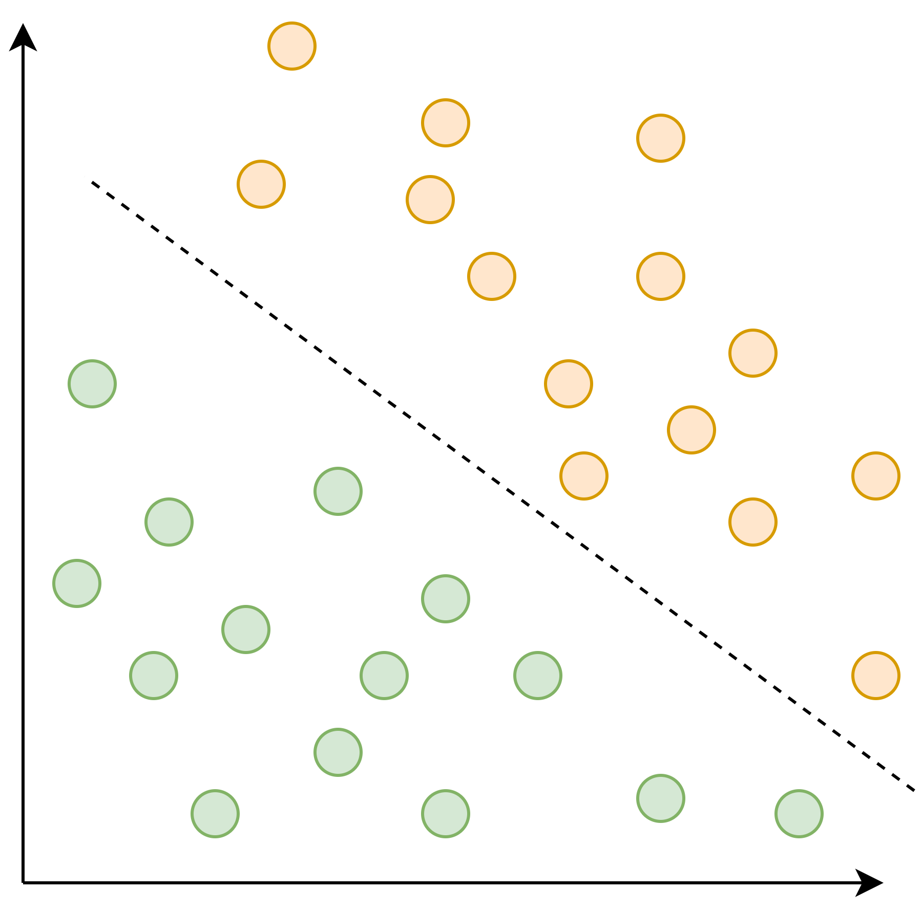
(a) Original data

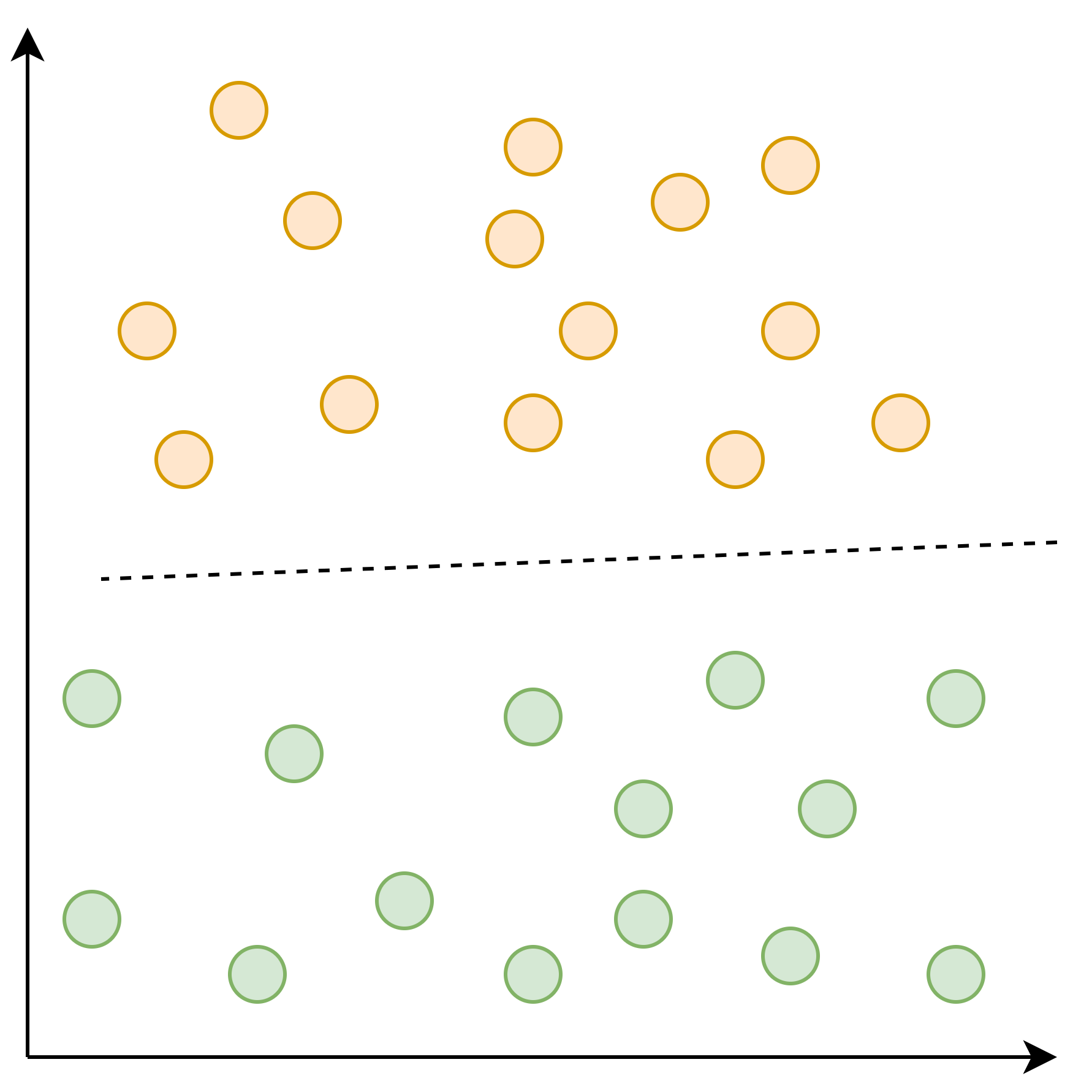
(b) Real drift

(c) Virtual drift

(d) Rigorous drift

Figure 1: Sources of concept drift based on how they occur probabilistically. Different colors represent different classes and the dotted line is the decision boundary.

In this study, all algorithms are used with the default parameters provided by their respective publications. In the experiments, the baseline classifier starts a new prediction model when a concept drift is detected. We should also note that, since we use a supervised classifier in our experiments, LD3 indirectly uses the ground truth labels of the data stream as it processes the predicted labels of the classifier. The reason behind this is the lack of online unsupervised multi-label classifiers. Although there are previously developed unsupervised multi-label classifiers, they are not designed for online learning, such as Wang and Zhang’s work (Wang and Zhang, 2020). Therefore, we chose to use a supervised classifier.

In the following sections, we first describe the problem domain, the aim of the study, and introduce the previous work in Sections 2 and 3. Then, we propose our solution in Section 4. Lastly, in Sections 5 and 6, we discuss the evaluation methodology and present our results and discussions. Section 7 concludes the paper.

2 Problem Domain and Aim of the Study

Traditional multi-label data stream classifiers learn by performing the interleaved test-then-train method (Büyükçakir et al, 2018), i.e, prequential training, on a stream of incoming data. However, if there is a change in data distribution, a significant decrease in predictive performance is experienced since the classifier still uses the previously learned distribution in its predictions. A concept drift detector detects the change in data distribution and alerts the classifier so that it can start working on adaptation strategies, which increases the robustness of the classifier.

Concept drift is the change in the data distribution that occurs over time. Given a data stream $S_{0,t}={d_{0},...,d_{t}}$, in a time window $[0,t]$, where $d_{i}=(X_{i},y_{i})$ with $X_{i}$ being the features and $y_{i}$ being the labels of the i-th data instance, concept drift is (Gama et al, 2014):

$$\exists t:P_{t}(X,y)\neq P_{t+1}(X,y)$$ (1)

According to this definition, Lu et al (2018) describe three potential sources of concept drift:

• The change may happen due to a change in posterior probabilities $P_{t}(y|X)$, meaning, $P_{t}(y|X)\neq P_{t+1}(y|X)$. This is called real or actual drift and it usually results in a shift in the decision boundary, causing a significant decrease in effectiveness.

• If the cause of the change is $P_{t}(X)\neq P_{t+1}(X)$, while $P_{t}(y|X)=P_{t+1}(y|X)$, it is called a virtual drift because it does not cause a shift in the decision boundary.

• The final source is when the change occurs as both $P_{t}(y|X)$ and $P_{t}(X)$ change over time which is called rigorous drift (Gözüaçık and Can, 2021).

Figure 1 illustrates the three sources of concept drift along with the original distribution.

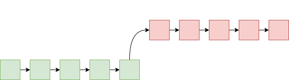
(a) Sudden drift

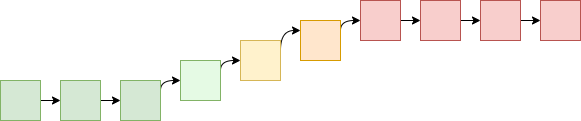
(b) Incremental drift

(c) Gradual drift

(d) Reoccurring concepts

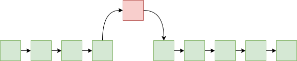
(e) Outlier

Figure 2: Types of concept drift based on what happens to the concept over time (outlier is not a drift). Different colors represent different concepts.

Lu et al (2018) further define four types of concept drift in terms of how they happen over time, which are illustrated in Figure 2. In the figure, the vertical axis represents data distribution and the horizontal axis represents time. Depending on the nature of data, this change may be sudden, incremental, gradual, or reoccurring. For example, with the changing of seasons, climate data may show reoccurring concepts or big events may cause sudden drift in news data.

Among the types presented in Figure 2, outlier is not actually a drift type. Outliers usually happen as a result of noise in the data. As they are false positives, a drift detector should also account for their presence to maintain accurate detection.

In this study, we aim to design an unsupervised concept drift detector and measure its boosting impact in classifier prediction accuracy. Our method LD3 exploits dependencies among predicted labels and grants drift detection capabilities to multi-label stream classifiers with no drift detection facility. In this work, we consider a supervised classification environment. The use of LD3 with an unsupervised multi-label (Wang and Zhang, 2020) or a self-tuning classifier (Roseberry and Cano, 2018) is beyond the scope of this paper.

Table 1: Error rate-based drift detection algorithm characteristics (They are all our baselines; for those with more than one version, the number of variants is given in parentheses after the detector name). The symbols $w_{hist}$ and $w_{new}$ indicate the windows for old and new data in respective order. Landmark uses the entire set of data before drift and flushes this data when drift is detected to collect the new distribution.

Category	Detector	Data Retrieval	Test Statistics	Hypothesis Test
Error rate-based	ADWIN Bifet and Gavalda (2007)	Auto cut $w_{hist}$, $w_{new}$	Error rate difference	Hoeffding’s Bound
	DDM Gama et al (2004)	Landmark	Online Error Rate	Distribution Estimation
	EDDM Baena-Garcıa et al (2006)	Landmark	Online Error Rate	Distribution Estimation
	FHDDM Pesaranghader and Viktor (2016)	Sliding $w_{hist}$, $w_{new}$	Correct prediction probability	Hoeffding’s Bound
	FHDDMS (2) Pesaranghader et al (2018a)	Stacked windows	Correct prediction probability	Hoeffding’s Bound
	HDDM (2) Frías-Blanco et al (2014)	Landmark	Online Error Rate	Hoeffding’s Bound
	KSWIN Raab et al (2020)	Sliding $w_{hist}$, $w_{new}$	Distribution distance	KS-Test
	MDDM (3) Pesaranghader et al (2018b)	Sliding $w_{hist}$, $w_{new}$	Weighted mean difference	McDiarmid’s Bound
	RDDM Barros et al (2017)	Landmark	Online Error Rate	Distribution Estimation
	SeqDrift2 Pears et al (2014)	Sliding $w_{hist}$, $w_{new}$	Online error rate	Bernstein Bound
Data distribution-based	LD3 (Our method)	Sliding $w_{hist}$, $w_{new}$	Rank correlation	Distribution Estimation

3 Related Works

In the following subsections, we first briefly introduce previously developed supervised detection algorithms based on online error rate monitoring and multi-label specific algorithms. Then, previous work on some of the unsupervised concept drift detection algorithms is presented.

3.1 Supervised Concept Drift Detection Algorithms

Concept drift is a prevalent problem in data stream mining, where many detectors are proposed to combat it within the literature. Based on previously developed algorithms, Lu et al (2018) propose an overall framework for concept drift detection which is comprised of four stages: Data retrieval, data modeling, test statistics calculation, and the hypothesis test. They further divide the detectors into three categories: Error rate-based, data distribution-based, and the multiple hypothesis test. Among these three, we focus on the first category as we were unable to find available source codes for multiple hypothesis test algorithms and data distribution-based algorithms. Table 1 displays the categories and methods used for each baseline algorithm we tested. The data modeling stage is not included in the table since all of the detectors except LD3 share the same data modeling scheme which is learner-based modeling.

3.1.1 Error Rate-based Algorithms

The detection algorithms in this category usually focus on the changes in the online error rate of the base classifiers, i.e, whether changes in the error rate of a classifier are statistically significant enough, the detector concludes that there is drift. Since these detectors monitor the online error rate and related metrics, they usually employ learners to model the data, which is the case for all of the algorithms presented in Section 3.1.1, and they tend to be efficient algorithms due to the simplicity of their input data (error-rate).

One of the most frequently used algorithms is the Drift Detection Method (DDM) proposed by Gama et al (2004). It uses a separate classifier to check whether the change in the online error rate is significant enough, which is done through distribution estimation. If the change is statistically significant, drift is detected. There are also a large number of algorithms that build upon the DDM algorithm, which usually change the test statistics and hypothesis test stages. For instance, Early Drift Detection Method (EDDM) (Baena-Garcıa et al, 2006) improves DDM by also considering the sample-wise distance between erroneous classifications.

In order to improve the hypothesis test stage, Frías-Blanco et al (2014) propose HDDM, which utilizes Hoeffding’s inequality (Hoeffding, 1963) to obtain probabilistic guarantees to further increase effectiveness. It has two variants, namely HDDM_A and HDDM_W, where, in the former, they use bounded moving averages (A-test) and in the latter, they use bounding weighted moving averages (W-test). Furthermore, Pesaranghader and Viktor (2016) introduce Fast Hoeffding Drift Detection Method (FHDDM) which requires the base detectors to either stay at a steady level or improve in accuracy. FHDDM checks this by monitoring the most recent probability of correct predictions instead of the error rate. Pesaranghader et al (2018a) further improve FHDDM as FHDDMS by adopting a stacking window scheme of various sizes. The stacking windows are a short and long window that has overlapping content that is used to detect sudden and gradual drifts separately. It also has another variant, FHDDMS_add, where the authors employ additive summaries for better efficiency in memory and execution time.

Apart from Hoeffding’s inequality-based improvements to DDM, Pesaranghader et al (2018b) developed McDiarmid Drift Detection Method (MDDM). MDDM is similar to HDDM as they also make improvements in hypothesis testing, by including the McDiarmid inequality to check the statistically significant differences. MDDM also implements a weighting scheme within its window where the most recent elements are given more importance. According to alternate weighting, it has three variants: MDDM_A (Arithmetic weighting), MDDM_E (Euler weighting), and MDDM_G (Geometric weighting).

Instead of modifying a stage, Barros et al (2017) propose Reactive Drift Detection Method (RDDM), in which they define a type of soft concept drift based on the number of samples accumulated in the window, called RDDM drift. RDDM re-calculates their DDM-based statistics to solve problems that arise from the high number of accumulated samples in the window.

Aside from DDM-based detectors, Bifet and Gavalda (2007) introduce ADWIN, which monitors the difference in error rate between two adaptive windows. The difference is bounded by Hoeffding’s inequality and if the difference exceeds the Hoeffding bound, a drift is detected.

Furthermore, Pears et al (2014) propose SeqDrift2. It employs an adapting sampling strategy to sample data from a window to get old and new concepts. Then, they detect the drift by comparing the differences according to the Bernstein bound.

Finally, Raab et al (2020) introduce KSWIN, which detects concept drift by applying “the Kolmogorov-Smirnov test” (KS-Test) which finds the distance between the estimated data distribution and the empirical distribution. These two distributions in KSWIN’s case would be the error rates stored in a sliced sliding window for new and old data. If the distance between the distributions exceeds the confidence interval, a drift is detected.

3.1.2 Algorithms for Multi-label Concept Drift Detection

In the multi-label classification problem domain, concept drift detection is a very thinly researched area. To the best of our knowledge, there are two previously developed concept drift detectors. However, in both cases the authors did not provide source codes thus we were unable to compare our results with them which is the reason why we did not include them in Table 1.

Shi et al (2014) propose a method in which they use label grouping and class entropy to detect concept drift. Initially they group the labels using clustering methods. Then for each label group, they calculate the multi-label entropy values within two sliding windows where they apply a threshold method to detect concept drift.

Wang et al (2020) introduce DDM-FP-M, a multi-label focused concept drift detector aimed at data streams on the Internet of Things problem domain. They propose modifications to DDM in which they add false positive classifications to make it more suitable for multi-labeled data stream environments.

3.2 Unsupervised Concept Drift Detection

Although many concept drift detectors exist, one area that is insufficiently researched is unsupervised concept drift detection. Iwashita and Papa (2018) found that unsupervised drift detectors only make up 3% of developed concept drift detectors. However, as Gemaque et al. point out, many of the real-world problems are better suited for unsupervised drift detection, since the swift acquisition of labels is often not possible (Gemaque et al, 2020). Since concept drift detection requires fast detection to enable rapid recovery after drift, the topic of unsupervised concept drift detection requires more attention.

Some of the previous works on unsupervised concept drift detection include detectors such as IKS-bdd (dos Reis et al, 2016), CD-TDS (Koh, 2016), Plover (de Mello et al, 2019), DSDD (Pinagé et al, 2020), D3 (Gözüaçık et al, 2019), and OCDD (Gözüaçık and Can, 2021).

IKS-bdd applies the Incremental Kolmogorov-Smirnov test, which is a modified Kolmogorov-Smirnov test that is better suited for online learning, to each of the data features in order to detect drift. CD-TDS detects two types of drift: Local drift and global drift. For local detection, the sample means of the new and old data are compared, bounded by the Hoeffding Bound. In the case of global drift, a pairwise statistical test is applied to find differences between two tree structures representing new and old data.

Plover monitors the input data behavior and detects changes based on observed instabilities. Moreover, DSDD detects drifts based on classification error simulation using an ensemble of classifiers.

Furthermore, Gözüaçık et al. introduce D3, a drift detector that utilizes a discriminative classifier that is trained on auto labeled samples based on how recent a sample was seen within a window (“0” for old and “1” for new samples). Drift detection is made by measuring the AUC score of the classifier. Likewise, OCDD uses a one-class classifier to distinguish between changing concepts, in which drift is detected when the ratio of false predictions is higher than a threshold.

Our work proposes an unsupervised drift detection algorithm that utilizes the predicted labels of the paired classifier; however, we were unable to compare our detector with the described unsupervised algorithms, excluding D3 and OCDD, as we could not find readily available source code.

Furthermore, D3 and OCDD are not compared with LD3 since we only used original codes provided by the frameworks we used. The provided source codes are incompatible with multi-label classification and we chose not to modify the original code for this reason.

4 Our Method: Label Dependency Drift Detector

In this study, we propose LD3, a data distribution-based, unsupervised concept drift detector which exploits the dependencies among predicted labels. It works alongside any online multi-label classifier that does not have inherent drift detection properties to assist in handling the changes in data distribution. We evaluate the changes in the label dependencies through the predicted labels provided by the paired model, and if a significant change occurs in the dependencies, we detect concept drift. In the remainder of this section, Algorithm 1 is referenced for explanations.

Table 2: Symbols table for Algorithm 1.

Symbol	Description
$l$	Predicted label
$L$	Threshold for number of anomalies
$t$	Standard deviation multiplier
$w$	Number of samples in a window
$W_{new}$	Label window for new samples
$W_{old}$	Label window for old samples
$W_{corr}$	Past correlation window

Algorithm 1 LD3: Label Dependency Drift Detector

Initialize $W_{new}$, $W_{old}$ and $W_{corr}$ as $\emptyset$

procedure LD3($l$, $t$, $w$, $L$)

     $drift$ $\leftarrow$ False

     $l^{\prime}\leftarrow$ Insert_Element($l$, $W_{new}$) $\quad\cdot\quad\cdot\quad\cdot\quad\cdot\quad\cdot\quad\cdot\quad\cdot\quad\cdot\quad\cdot\quad\cdot\quad\cdot\quad\cdot\quad\cdot\quad\cdot\quad$ $\ignorespaces\triangleright$ $l^{\prime}$ is the last element removed

     if $|W_{new}|$ = $w$ then

         Insert_Element($l^{\prime}$, $W_{old}$)

     end if

     if $|W_{new}|$ $\neq$ $w$ and $|W_{old}|$ $\neq$ $w$ then

         return $drift$

     else

         $M_{new}$ $\leftarrow$ Co-occurrence matrix created from $W_{new}$

         $M_{old}$ $\leftarrow$ Co-occurrence matrix created from $W_{old}$

         $R_{new}$ $\leftarrow$ Reciprocal ranking of $M_{new}$ $\quad\cdot\quad\cdot\quad\cdot\quad\cdot\quad\cdot\quad\cdot\quad\cdot\quad\cdot\quad\cdot\quad\cdot\quad\cdot\quad\cdot\quad$ $\ignorespaces\triangleright$ Global ranking for $W_{new}$

         $R_{old}$ $\leftarrow$ Reciprocal ranking of $M_{old}$ $\quad\cdot\quad\cdot\quad\cdot\quad\cdot\quad\cdot\quad\cdot\quad\cdot\quad\cdot\quad\cdot\quad\cdot\quad\cdot\quad\cdot\quad\cdot$ $\ignorespaces\triangleright$ Global ranking for $W_{old}$

         $C$ $\leftarrow$ WS($R_{new}$, $R_{old}$) $\quad\cdot\quad\cdot\quad\cdot\quad\cdot\quad\cdot\quad\cdot\quad\cdot\quad\cdot\quad\cdot\quad\cdot\quad\cdot\quad\cdot\quad\cdot$ $\ignorespaces\triangleright$ Rank Correlation of $R_{new}$ and $R_{old}$

         Insert_Element($C$, $W_{corr}$)

         if $|W_{corr}|$ $\neq$ $w$ then

              return $drift$

         end if

         $len\leftarrow$ Sigma_Rule($W_{corr}$, $t$) $\quad\cdot\quad\cdot\quad\cdot\quad\cdot\quad\cdot\quad\cdot\quad\cdot\quad\cdot\quad\cdot\quad\cdot\quad\cdot\quad\cdot\quad\cdot$ $\ignorespaces\triangleright$ Number of anomalies in $W_{corr}$

         if $len>L$ then

              $drift\leftarrow$ True

              Clear windows $W_{new},W_{old},W_{corr}$

         end if

     end if

     return $drift$

end procedure

4.1 Evaluating the Changes in the Label Dependencies

In an ideal environment, labels can be chosen such that each label is independently distributed, i.e, dependencies do not exist. However, in real-world datasets, this is usually not the case, as some labels tend to occur more frequently together (e.g, in movie categories, comedy and drama tags occur more commonly together than comedy and thriller tags). In our study, we hypothesize that this correlation causes dependencies, and changes in these dependencies are a precursor to concept drift.

Given a multi-label classifier, we buffer the labels predicted by the classifier in two fixed-sized moving windows, one each for the new and old data. Apart from providing up-to-date statistics about label distribution, these windows allow the classifier to boot itself up, i.e, learn enough of the data distribution to generate consistent predictions, as the windows are filled (Alg. 1, lines 4-6), which functions as a warmup scheme.

After the windows are full, we first generate two co-occurrence matrices from the windows (Alg. 1, lines 10-11). The matrices are obtained by counting the number of times each class label occurs as “1” alongside other labels. The generated matrices are then ranked within each row, which we call local ranking, by creating a ranking for each label based on their co-occurrence frequencies.

Following the local ranking, the ranks are aggregated by utilizing a data fusion algorithm to obtain a representation of label dependencies for new and old samples (Alg. 1, lines 12-13). We call the resulting aggregated ranking as global ranking. Through this, we obtain the most influential labels among all of them and use these labels to monitor changes in the stream. We use reciprocal rank fusion, which is seen in Equation 2, where $r_{i}$ is the global ranking of a class label within the predicted label $l$, which is denoted by $l_{i}$. Moreover, we use $n$ to represent the number of classes and $r_{ij}$ for the local ranking of $l_{i}$, where $\{j\,|\,1\leq j\leq n\}$. We justify our selection of reciprocal rank fusion, rather than some other commonly used approaches, by experiments in Section 6.3.

$$r_{i}=\frac{1}{\sum_{j=1}^{n}\frac{1}{r_{ij}}}\qquad\{i\,|\,1\leq i\leq n\}$$ (2)

4.2 Measuring Similarity Between Two Rankings

Subsequent to the global ranking, we calculate the rank correlation between the two global rankings we obtained (Alg. 1, line 14), which evaluates the similarity between rankings. We use the WS coefficient as our rank correlation measure which is a ranking similarity method developed by Sałabun and Urbaniak (2020). It calculates the weighted similarity between two rankings and returns a value bounded within $[-1,1]$, where two identical rankings are scored as 1, whereas the score is -1 for the opposite case, from which can be deduced Equation 3. In this equation, $R_{xi}$ and $R_{yi}$ represent the rank position of a label $l_{i}$ within $R_{new}$ and $R_{old}$.

$$C=1-\sum_{i=1}^{n}\left(2^{-R_{xi}}\cdot\frac{|R_{xi}-R_{yi}|}{max\{|1-R_{xi}|,|n-R_{xi}|\}}\right)$$ (3)

Within the summation, $2^{-R_{xi}}$ is the weight of the label $l_{i}$ which ensures that higher ranking labels have more influence. The numerator $|R_{xi}-R_{yi}|$ is the ranking distance of $l_{i}$ within the two rankings and the denominator scales this distance.

We chose to use the WS coefficient instead of other popular rank correlation measures such as Kendall’s $\tau$ (Kendall, 1938) or Spearman’s $\rho$ (Spearman, 1987) because it provides a way to weigh the labels. Since we measure the influences labels have on each other, a change in the higher ranked labels is more important than other labels. Furthermore, it measures the similarity based on the distance between the two rankings. In a possibly volatile environment like a data stream, rankings could change by a few places temporarily; however, if we measure the similarity based on distance, such irregularities are tolerated more easily, which is why measures such as weighted $\tau$ (Vigna, 2015) are not suitable for our case.

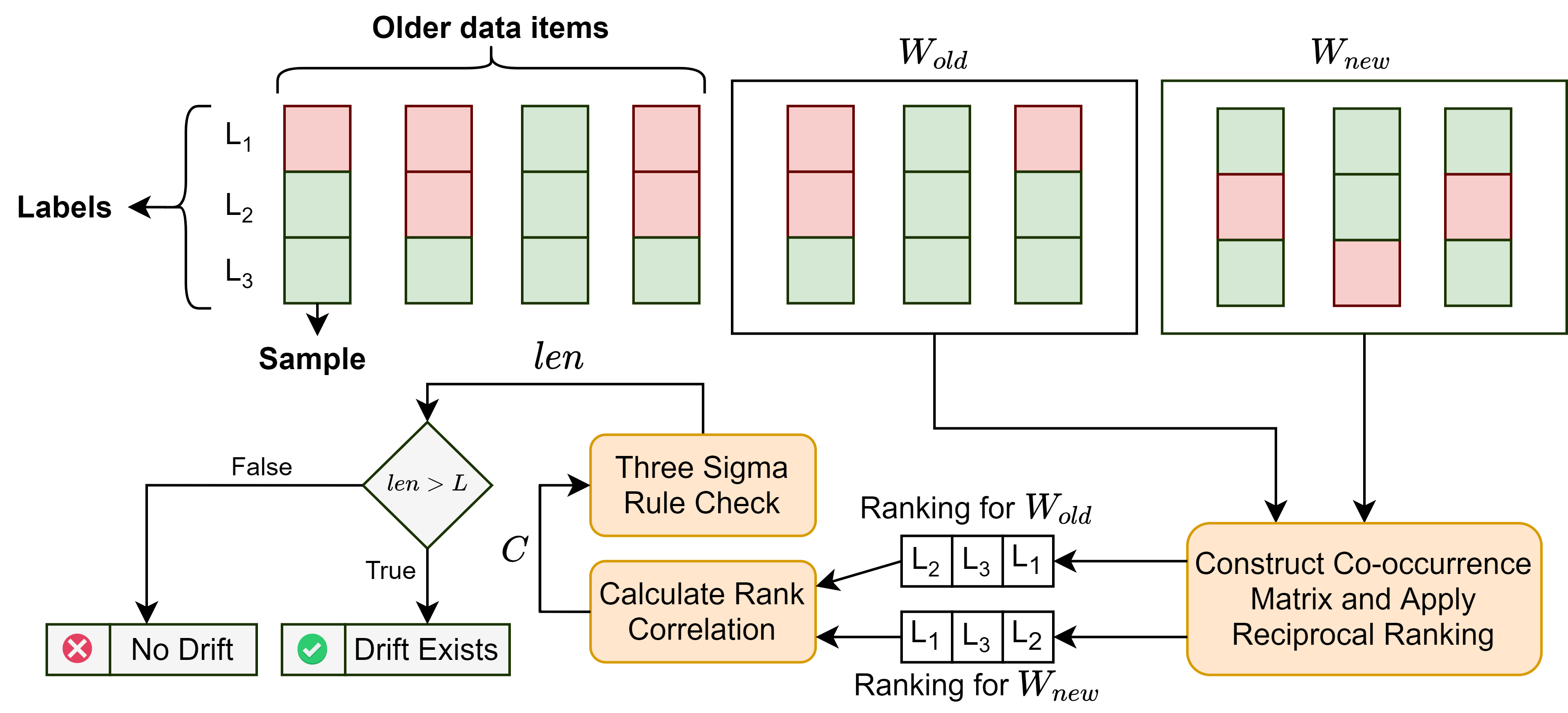
Figure 3: Workflow of LD3. Red boxes represent false labels (0) and green boxes represent true labels (1).

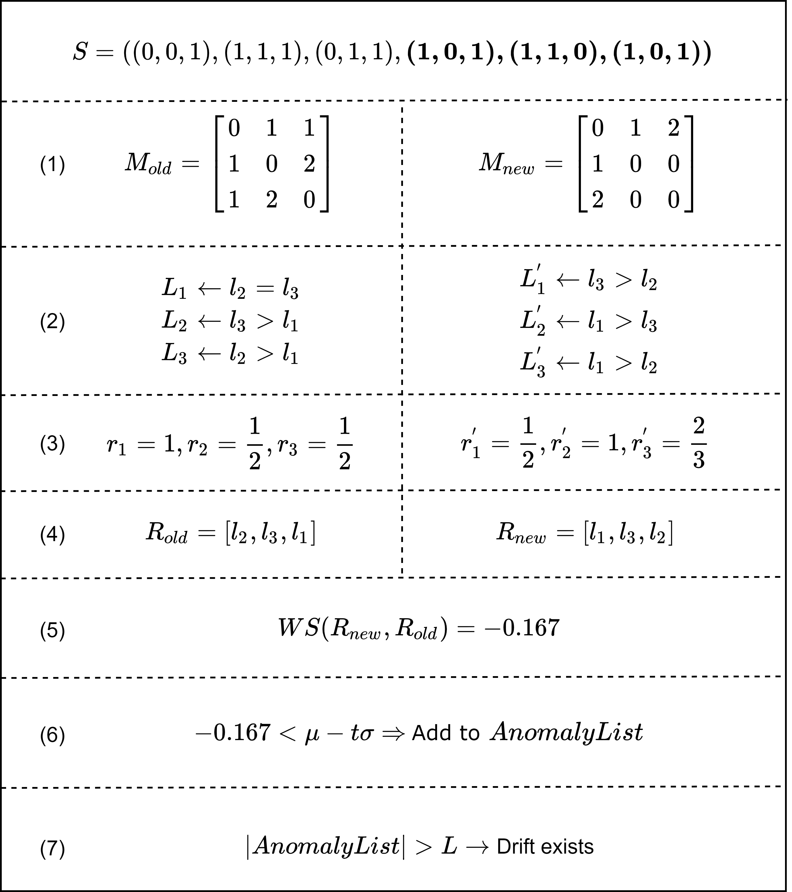
Figure 4: A simple numerical example of LD3 where $\mu$ and $\sigma$ are the mean and standard deviation of the samples within $W_{corr}$, t is the standard deviation multiplier for the three sigma rule (Pukelsheim, 1994), and L is the number of anomalies threshold. Recently arrived predicted labels are highlighted in bold. The calculations are explained in more detail in Appendix A.

Although the generated rank correlation value implies whether the current ranking indicates a drift, it needs to be checked for statistical significance. This is done by utilizing the three sigma rule (Pukelsheim, 1994), which translates to a simple left tailed test for our case (Alg. 1, line 15-19). A separate moving window ($W_{corr}$) is utilized to accumulate the past rank correlations. If the current correlation is less than the mean ($\mu$) within the window by $t$ times the standard deviation ($\sigma$), it is considered an anomaly. However, such anomalies may be the result of noise in the data, i.e, outliers described in Section 2. To prevent false detections, we store these anomalies in a list, and if the length of this list is greater than a chosen length $L$, the detector signals that a drift has been encountered. The three sigma rule is used here to increase the computational efficiency of the algorithm as the desired result is obtained without having to estimate the distribution of the recent data in its entirety.

The general representation of all of the stages is illustrated in Figure 3. In addition, a simple numerical example of LD3 is given in Figure 4. In this figure, $M_{old}$ and $M_{new}$ are obtained by counting the co-occurrences of labels. Then, local rankings are obtained which are represented as $L_{i}$ and $L^{\prime}_{i}$ for each label within $M_{old}$ and $M_{new}$. The variables $r_{i}$ and $r^{\prime}_{i}$ are reciprocal ranking results for old and new samples for each label.

5 Evaluation and Experimental Setup

5.1 Datasets

For evaluation, we used nine well-known real-world multi-label datasets, which we obtained in MEKA (Read et al, 2016) formats, and three synthetic data streams (Montiel et al, 2018). Table 1 represents the datasets and their properties. The datasets are chosen among the ones tested in the study of Roseberry and Cano (2018). We used all datasets from that list shown to have drift by any of the tested detectors and had better effectiveness results than a baseline classifier without drift detection functionalities. Since we measure the detectors’ benefit based on the effectiveness improvement on the classifier, if the baseline classifier shows higher predictive performance, we conclude that detectors only make false positive detections. In such a case, we assume the dataset does not have drift.

Table 3: Table of multi-label datasets used in the experiments. The upper group contains the real-world datasets. $N$ represents the number of samples, $D$ is the number of features, $n$ is the number of labels and LC($\mathcal{D}$) and LD($\mathcal{D}$) represents label cardinality and label density which are the average number of true labels of the samples in dataset $\mathcal{D}$ and LC($\mathcal{D}$) divided by the number of labels, indicating the average label cardinality per label (Tsoumakas and Katakis, 2007).

Dataset Name	Domain	$N$	$D$	$n$	LC($\mathcal{D}$)	LD($\mathcal{D}$)
20NG	Text	19,300	1,006	20	1.029	0.051
Birds	Audio	645	260	19	1.014	0.053
Enron	Text	1,702	1,001	53	3.378	0.064
EukaryotePseAAC	Biology	7,766	440	22	1.146	0.052
Imdb	Text	120,900	1,001	28	2.000	0.071
Ohsumed	Text	13,930	1,002	23	1.663	0.072
PlantPseAAC	Biology	978	440	12	1.079	0.090
Tmc2007-500	Text	28,600	500	22	2.220	0.101
Yeast	Biology	2,417	103	14	4.237	0.303
Synthetic Sudden Drift	Generic	20,000	200	50	1.587	0.0397
Synthetic Incremental Drift	Generic	20,000	200	50	1.588	0.0397
Synthetic Re-occurring Drift	Generic	20,000	200	50	1.588	0.0397

The three synthetic data streams are generated to measure the difference in effectiveness results among sudden, incremental, and reoccurring drifts, which are generated by changing between three different multi-label data streams that have different label cardinalities (for reoccurring concepts, the third data stream has the same properties and data distribution as the first data stream). The change between streams is smoothed by the sigmoid function over a specified amount of samples. To simulate sudden drift, we applied the change over one sample whereas in the reoccurring and incremental drifted streams the change is applied over 500 samples. The data streams have 20,000 samples and the drifts are at sample positions 4,000 and 10,000. The properties of the streams are shown in Table 1.

5.2 Experimental Setup and Evaluation Metrics

The experiments are performed using the Scikit-Multiflow (Montiel et al, 2018) and Tornado (Pesaranghader et al, 2018a) frameworks. Scikit-multiflow is employed for synthetic data stream generation and it contains six (ADWIN, DDM, EDDM, HDDM_A, HDDM_W, KSWIN) of the tested baseline detectors. Moreover, the Tornado framework is utilized as it contains the remaining eight baseline detectors.

To demonstrate the effectiveness benefits of the detectors, a Classifier Chain (CC) (Read et al, 2011) using Gaussian Naive Bayes (NB) classifiers (John, 1995) is used as a base classifier. CCs build binary classifiers for each class label that are linked in a chain to preserve inter-label dependencies. The reason for using a CC is that it provides accurate results with reasonably fast execution. The same reasoning applies to the use of NBs as base classifiers and it is also a popular base classifier that is frequently used in the literature (Pintas et al, 2021). Furthermore, our concept drift adapting strategy resets the classifier if drift is detected.

Gama et al (2014) propose three possible metrics for change detection algorithms: (1) Probability of true change detection, (2) Probability of false alarms, and (3) Delay of detection. In our experiments and discussions, in order to incorporate the suggested measures, we first perform effectiveness tests on the 12 datasets we presented. Then, through plots, we make an in-depth analysis on the obtained effectiveness measures on the top four performing detectors, in which we discuss the effects of the false detections (alarms) and true detections. Lastly, to measure the impact of detection delay, we perform experiments using six synthetic data streams with varying drift speeds, i.e, how fast does the change happen between old and new concepts. This experiment allows us to assess the detectors’ response within different drift environments.

Table 4: Experiment results for the detectors. ND is a classifier without any detection methods for the baseline. Average result is calculated from the average result of each algorithm, except LD3, for a dataset. LD3 Imp. represents LD3’s improvement over the average. Avg. Imp. illustrates the average improvement for each metric. The best results are highlighted in bold.

(a) Example-based accuracy and Hamming score results

Detector	20NG	Birds	Enron	Eukatyote PseAAC	Imdb	Ohsumed	Plant PseAAC	Tmc2007- 500	Yeast	Synthetic Incremental	Synthetic Reoccurring	Synthetic Sudden	Average Rank
Example-based Accuracy
LD3	0.1616	0.0992	0.1403	0.1946	0.1140	0.0693	0.3198	0.2029	0.3780	0.0788	0.0808	0.0788	1.00
ADWIN	0.1386	0.0550	0.1245	0.0327	0.1093	0.0361	0.1431	0.1962	0.3622	0.0724	0.0730	0.0724	8.46
DDM	0.0525	0.0550	0.1255	0.0327	0.0799	0.0364	0.1126	0.1529	0.3557	0.0749	0.0759	0.0749	10.58
EDDM	0.0654	0.0550	0.1355	0.0327	0.0894	0.0368	0.1272	0.1593	0.3707	0.0787	0.0762	0.0744	6.25
FHDDM	0.1453	0.0550	0.1236	0.0327	0.0797	0.0381	0.1240	0.1555	0.3622	0.0659	0.0761	0.0659	9.83
FHDDMS	0.1444	0.0550	0.1236	0.0327	0.0797	0.0381	0.1136	0.1555	0.3622	0.0659	0.0761	0.0659	10.42
FHDDMS_Add	0.1483	0.0550	0.1239	0.0327	0.0797	0.0373	0.1165	0.1555	0.3622	0.0659	0.0761	0.0659	90.956
HDDM_A	0.1505	0.0550	0.1371	0.0327	0.0797	0.0367	0.1235	0.1555	0.3622	0.0698	0.0761	0.0722	8.08
HDDM_W	0.1469	0.0550	0.1371	0.0327	0.0797	0.0367	0.1070	0.1555	0.3622	0.0659	0.0761	0.0659	9.79
KSWIN	0.1438	0.0550	0.1245	0.0327	0.0797	0.0590	0.1793	0.1555	0.3622	0.0659	0.0761	0.0659	8.67
MDDM_A	0.1396	0.0550	0.1237	0.0327	0.0797	0.0381	0.1218	0.1555	0.3622	0.0659	0.0761	0.0659	10.25
MDDM_E	0.1419	0.0550	0.1242	0.0327	0.0797	0.0381	0.1180	0.1555	0.3622	0.0659	0.0761	0.0659	10.00
MDDM_G	0.1419	0.0550	0.1242	0.0327	0.0797	0.0381	0.1180	0.1555	0.3622	0.0659	0.0761	0.0659	10.00
RDDM	0.1562	0.0574	0.1237	0.1225	0.1130	0.0382	0.2225	0.2016	0.3622	0.0722	0.0746	0.0720	5.38
SEQDRIFT2	0.1190	0.0550	0.1283	0.0327	0.0797	0.0363	0.1709	0.1555	0.3622	0.0717	0.0739	0.0750	9.25
ND	0.1469	0.0550	0.1371	0.0327	0.0797	0.0608	0.1369	0.1555	0.3622	0.0659	0.0761	0.0659	8.08
Average Result	0.1321	0.0552	0.1278	0.0387	0.0846	0.0403	0.1357	0.1614	0.3623	0.0689	0.0756	0.0689	Avg. Imp.
LD3 Imp. (%)	22.3	79.7	9.8	402.8	34.8	72.0	135.7	25.7	4.3	14.4	6.9	14.4	68.6
Hamming Score
LD3	0.8578	0.7302	0.8033	0.7979	0.7673	0.8023	0.8559	0.7340	0.7193	0.8098	0.7670	0.8306	1.50
ADWIN	0.8426	0.4996	0.7428	0.5773	0.7499	0.6520	0.7765	0.6867	0.6970	0.7396	0.7342	0.7408	6.67
DDM	0.2271	0.4996	0.7398	0.5773	0.7000	0.1627	0.5688	0.5019	0.7087	0.8283	0.8016	0.7888	10.17
EDDM	0.5486	0.4996	0.7594	0.5773	0.7039	0.4412	0.5984	0.6007	0.7221	0.7969	0.7743	0.7830	8.00
FHDDM	0.8550	0.4996	0.7423	0.5773	0.7088	0.7520	0.6887	0.5069	0.6970	0.6773	0.6971	0.6781	9.21
FHDDMS	0.8599	0.4996	0.7423	0.5773	0.7088	0.7485	0.6463	0.5069	0.6970	0.6773	0.6971	0.6781	9.67
FHDDMS_Add	0.8340	0.4996	0.7404	0.5773	0.7088	0.7490	0.6575	0.5069	0.6970	0.6773	0.6971	0.6781	10.54
HDDM_A	0.8069	0.4996	0.7632	0.5773	0.7088	0.4764	0.6022	0.5069	0.6970	0.7026	0.6971	0.7412	9.38
HDDM_W	0.7953	0.4996	0.7632	0.5773	0.7088	0.5013	0.5768	0.5069	0.6970	0.6773	0.6971	0.6781	10.58
KSWIN	0.8343	0.4996	0.7445	0.5773	0.7088	0.6916	0.7489	0.5069	0.6970	0.6773	0.6971	0.6781	9.46
MDDM_A	0.8518	0.4996	0.7415	0.5773	0.7088	0.7520	0.6835	0.5069	0.6970	0.6773	0.6971	0.6781	9.67
MDDM_E	0.8504	0.4996	0.7428	0.5773	0.7088	0.7523	0.6714	0.5069	0.6970	0.6773	0.6971	0.6781	9.29
MDDM_G	0.8504	0.4996	0.7428	0.5773	0.7088	0.7524	0.6714	0.5069	0.6970	0.6773	0.6971	0.6781	9.21
RDDM	0.8696	0.5140	0.7417	0.6560	0.7654	0.7669	0.7847	0.7227	0.6970	0.7272	0.7117	0.7286	4.58
SEQDRIFT2	0.7942	0.4996	0.7421	0.5773	0.7088	0.6304	0.7763	0.5069	0.6970	0.7266	0.7327	0.7778	8.83
ND	0.7953	0.4996	0.7632	0.5773	0.7088	0.6685	0.8168	0.5069	0.6970	0.6773	0.6971	0.6781	9.25
Average Result	0.7744	0.5006	0.7475	0.5825	0.7144	0.6332	0.6845	0.5392	0.6995	0.7078	0.7150	0.7109	Avg. Imp.
LD3 Imp. (%)	10.8	45.9	7.5	37.0	7.4	26.7	25.0	36.1	2.8	14.4	7.3	16.8	19.8

Table 5: Continued.

(a) Example-based F1 score and Micro-averaged F1 score results

Detector	20NG	Birds	Enron	Eukatyote PseAAC	Imdb	Ohsumed	Plant PseAAC	Tmc2007- 500	Yeast	Synthetic Incremental	Synthetic Reoccurring	Synthetic Sudden	Average Rank
Example-based F1 Score
LD3	0.3173	0.1242	0.3496	0.4593	0.2240	0.1031	0.5596	0.4048	0.5299	0.1387	0.1719	0.1325	2.75
ADWIN	0.2999	0.1527	0.3150	0.1074	0.2077	0.0424	0.2479	0.3858	0.5204	0.1371	0.1455	0.1364	7.46
DDM	0.1207	0.1527	0.3017	0.1074	0.1424	0.0646	0.2547	0.3010	0.5072	0.1124	0.1201	0.1191	12.08
EDDM	0.1932	0.1527	0.3155	0.1074	0.1606	0.0557	0.2737	0.3458	0.5159	0.1236	0.1340	0.1265	8.17
FHDDM	0.2965	0.1527	0.3050	0.1074	0.1409	0.0424	0.2408	0.3024	0.5204	0.1210	0.1556	0.1211	10.38
FHDDMS	0.2915	0.1527	0.3050	0.1074	0.1409	0.0435	0.2253	0.3024	0.5204	0.1210	0.1556	0.1211	10.25
FHDDMS_Add	0.3024	0.1527	0.3077	0.1074	0.1409	0.0439	0.2283	0.3024	0.5204	0.1210	0.1556	0.1211	9.29
HDDM_A	0.3145	0.1527	0.3176	0.1074	0.1409	0.0530	0.2549	0.3024	0.5204	0.1264	0.1556	0.1386	6.46
HDDM_W	0.3099	0.1527	0.3176	0.1074	0.1409	0.0526	0.2104	0.3024	0.5204	0.1210	0.1556	0.1211	8.75
KSWIN	0.2893	0.1527	0.3030	0.1074	0.1409	0.0974	0.3273	0.3024	0.5204	0.1210	0.1556	0.1211	8.96
MDDM_A	0.2992	0.1527	0.3066	0.1074	0.1409	0.0426	0.2422	0.3024	0.5204	0.1210	0.1556	0.1211	9.79
MDDM_E	0.3040	0.1527	0.3065	0.1074	0.1409	0.0428	0.2375	0.3024	0.5204	0.1210	0.1556	0.1211	9.62
MDDM_G	0.3040	0.1527	0.3065	0.1074	0.1409	0.0428	0.2375	0.3024	0.5204	0.1210	0.1556	0.1211	9.62
RDDM	0.3021	0.1461	0.3029	0.3905	0.2239	0.0429	0.4141	0.3986	0.5204	0.1432	0.1536	0.1436	6.54
SEQDRIFT2	0.2828	0.1527	0.3241	0.1074	0.1409	0.0429	0.3099	0.3024	0.5204	0.1299	0.1410	0.1339	8.21
ND	0.3099	0.1527	0.3176	0.1074	0.1409	0.1044	0.2430	0.3024	0.5204	0.1210	0.1556	0.1211	7.67
Average Result	0.2813	0.1523	0.3102	0.1263	0.1523	0.0543	0.2632	0.3108	0.5192	0.1241	0.1500	0.1259	Avg. Imp.
LD3 Imp. (%)	12.8	-18.5	12.7	263.7	47.1	89.9	112.6	30.2	2.1	11.8	14.6	5.2	48.7
Micro-averaged F1 Score
LD3	0.2783	0.1804	0.2461	0.3258	0.2047	0.1297	0.4846	0.3374	0.5486	0.1462	0.1495	0.1461	1.00
ADWIN	0.2435	0.1043	0.2215	0.0633	0.1970	0.0697	0.2504	0.3280	0.5318	0.1351	0.1360	0.1351	8.42
DDM	0.0997	0.1043	0.2230	0.0633	0.1480	0.0702	0.2024	0.2652	0.5247	0.1393	0.1411	0.1393	10.58
EDDM	0.1227	0.1043	0.2387	0.0633	0.1641	0.0711	0.2257	0.2749	0.5409	0.1460	0.1417	0.1385	6.25
FHDDM	0.2537	0.1043	0.2200	0.0633	0.1476	0.0734	0.2206	0.2691	0.5318	0.1236	0.1414	0.1236	9.92
FHDDMS	0.2523	0.1043	0.2200	0.0633	0.1476	0.0735	0.2040	0.2691	0.5318	0.1236	0.1414	0.1236	10.29
FHDDMS_Add	0.2583	0.1043	0.2205	0.0633	0.1476	0.0719	0.2087	0.2691	0.5318	0.1236	0.1414	0.1236	9.96
HDDM_A	0.2616	0.1043	0.2411	0.0633	0.1476	0.0708	0.2199	0.2691	0.5318	0.1306	0.1414	0.1346	8.12
HDDM_W	0.2561	0.1043	0.2411	0.0633	0.1476	0.0709	0.1933	0.2691	0.5318	0.1236	0.1414	0.1236	9.75
KSWIN	0.2514	0.1043	0.2214	0.0633	0.1476	0.1115	0.3041	0.2691	0.5318	0.1236	0.1414	0.1236	8.71
MDDM_A	0.2450	0.1043	0.2201	0.0633	0.1476	0.0734	0.2171	0.2691	0.5318	0.1236	0.1414	0.1236	10.38
MDDM_E	0.2485	0.1043	0.2209	0.0633	0.1476	0.0734	0.2111	0.2691	0.5318	0.1236	0.1414	0.1236	10.08
MDDM_G	0.2485	0.1043	0.2209	0.0633	0.1476	0.0735	0.2111	0.2691	0.5318	0.1236	0.1414	0.1236	9.88
RDDM	0.2701	0.1087	0.2202	0.2183	0.2030	0.0736	0.3640	0.3356	0.5318	0.1348	0.1389	0.1344	5.33
SeqDrift2	0.2127	0.1043	0.2274	0.0633	0.1476	0.0700	0.2919	0.2691	0.5318	0.1338	0.1376	0.1395	9.25
ND	0.2561	0.1043	0.2411	0.0633	0.1476	0.1147	0.2408	0.2691	0.5318	0.1236	0.1414	0.1236	8.08
Average Result	0.2320	0.1046	0.2265	0.0736	0.1557	0.0774	0.2378	0.2776	0.5319	0.1288	0.1406	0.1289	Avg. Imp.
LD3 Imp. (%)	20.0	72.5	8.7	342.7	31.5	67.6	103.4	21.5	3.1	13.5	6.3	13.3	58.7

The tests are conducted using prequential evaluation (Gama et al, 2009). We apply the following four metrics to evaluate the effectiveness of the algorithms which are used in previous literature to measure multi-label classification effectiveness (Büyükçakir et al, 2018; Nam et al, 2017).

• Example-based metrics: Example-based accuracy (Eq. 4), Hamming score (Eq. 5), and example-based F1 score (Eq. 6). The formulas for these are given below in equations with $\hat{y}_{i}$ being the prediction, $Y_{i}$ as the ground truth, $n$ as the number of labels, and $N$ being the number of samples.

• Label-based metrics: Micro-averaged F1 score (Eq. 7). $TP_{i}$, $FP_{i}$, and $FN_{i}$ are true positive, false positive, and false positive counts for the i-th label (Zhang and Zhou, 2013).

$$Accuracy_{example}=\frac{1}{N}\sum^{N}_{i=1}\frac{|Y_{i}\bigcap\hat{y}_{i}|}{|Y_{i}\bigcup\hat{y}_{i}|}$$ (4)

$$HammingScore=1-\frac{1}{N}\sum^{N}_{i=1}\frac{1}{n}|\hat{y}_{i}\Delta Y_{i}|$$ (5)

$$F1_{example}=\frac{2\cdot Precision_{example}\cdot Recall_{example}}{Precision_{example}+Recall_{example}}$$ (6)

$$F1_{micro}=F1\left(\sum^{n}_{i=1}TP_{i},\sum^{n}_{i=1}FP_{i},\sum^{n}_{i=1}FN_{i}\right)$$ (7)

LD3 is compared with the detection algorithms displayed in Table 1 and their variations. Although these detection algorithms are not specifically designed for multi-label use-case, they are eligible baseline algorithms because they are error rate-based detectors. For this type of algorithms, the input passed into the detector is whether or not the prediction is correct, which means that their input is “1” for correct and “0” for false predictions (For “1”, all predicted labels must match exactly to the true labels). For this reason, they can also be used in the multi-label concept detection problem domain since this information is also generated in multi-label data streams. Wang et al (2020) also test their multi-label concept drift detection algorithm against DDM.

6 Experimental Results and Discussion

In the following subsections, we discuss and analyze our results based on effectiveness measures, provide simple guidelines for hyperparameter optimization, discuss the effects of different data fusion algorithms, and the influence of various drift types and speeds.

6.1 Effectiveness Analysis

We assess our effectiveness results by comparing our experimental results with the baseline detectors. Furthermore, we visually analyze the effectiveness results in the time scale. Lastly, we discuss the advantages of unsupervised detection with pointers on efficiency.

6.1.1 Analysis with Different Effectiveness Measures

The results of our experiments are presented in Table 2. Each row represents the results of a detector and columns represent the datasets. The table is divided into four sections for each effectiveness measure. The baseline classifier without a detector is labeled as “ND”, i.e, no detector. While calculating the average rankings, the ties are handled by averaging the ranks that would be assigned to all the tied values and assigning that value to each tied element, e.g., for the given list $[1,2,3,3,4]$, the average ranking is $[1,2,3.5,3.5,5]$.

The results show that LD3 achieves the best results overall on all metrics. For all metrics, LD3 achieves at least 19.8% improvement over the baseline averages. However, average rank-wise, LD3 displays comparatively worse predictive performance on the example-based F1 score than other metrics. We found that the reason behind this is mostly due to the classifier resetting procedure. Example-based F1 score punishes miss-classifications more harshly than example-based accuracy since miss-classified samples are multiplied in its numerator and they are divided by additive components. A recently reset classifier is prone to incorrect predictions and it is usually the case that none of the predicted labels match with the true labels for the first samples after resetting which produces the outcome of worse example-based F1 scores.

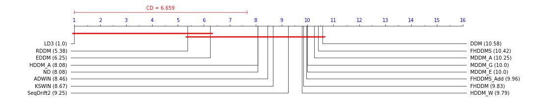
(a) Example-based accuracy

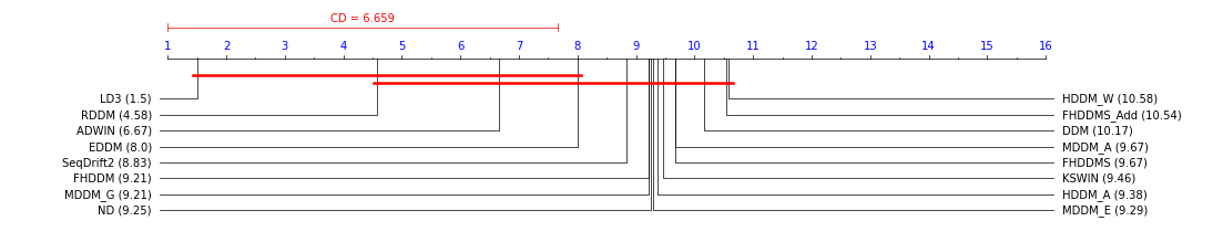
(b) Hamming score

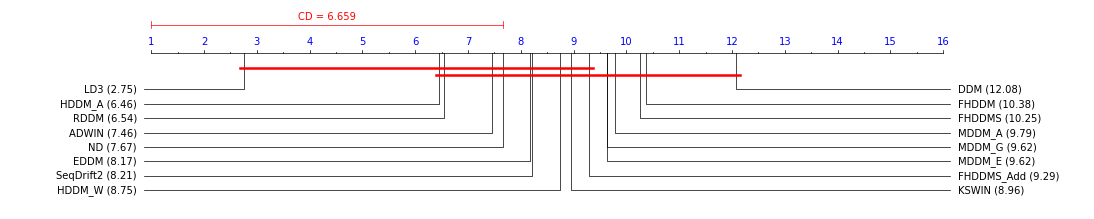
(c) Example-based F1 score

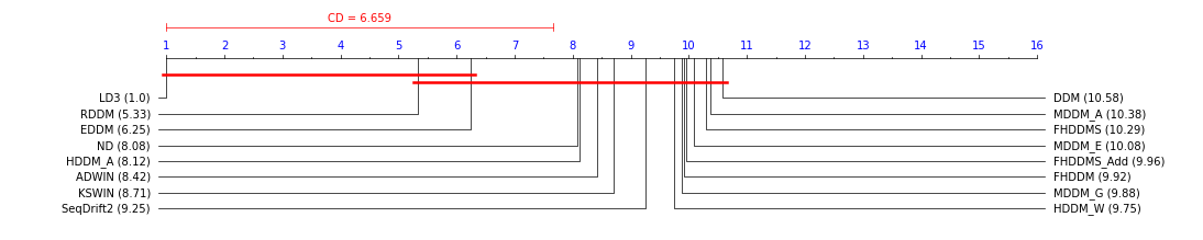
(d) Micro-averaged F1 score

Figure 5: Nemenyi critical distance diagrams for all metrics. The number given within parentheses after the method name indicates rank position of the method.

6.1.2 Statistical Significance Evaluation of Effectiveness Results

To further investigate the effectiveness of LD3, we performed the “Friedman test with Nemenyi post-hoc analysis” in which we evaluate the statistical significance of our results, which is presented in Figure 5. We applied the two-tailed Nemenyi test to find our critical distance for Nemenyi Significance. Our critical distance is $CD=6.659$, which is calculated using Equation 8, where $q_{\alpha,k}$ is the critical value acquired from the Critical Values Table from Demšar (2006) with $\alpha=0.05$ and $k$ is the number of algorithms (16) and $K$ is the number of datasets (12).

$$CD=q_{\alpha,k}\sqrt{\frac{k(k+1)}{6K}}$$ (8)

The Nemenyi Significance tests show that LD3 achieves the overall best rankings with a statistically significant difference from most of the detectors. Among the different effectiveness measures, only RDDM and EDDM consistently display statistically indistinguishable predictive performance.

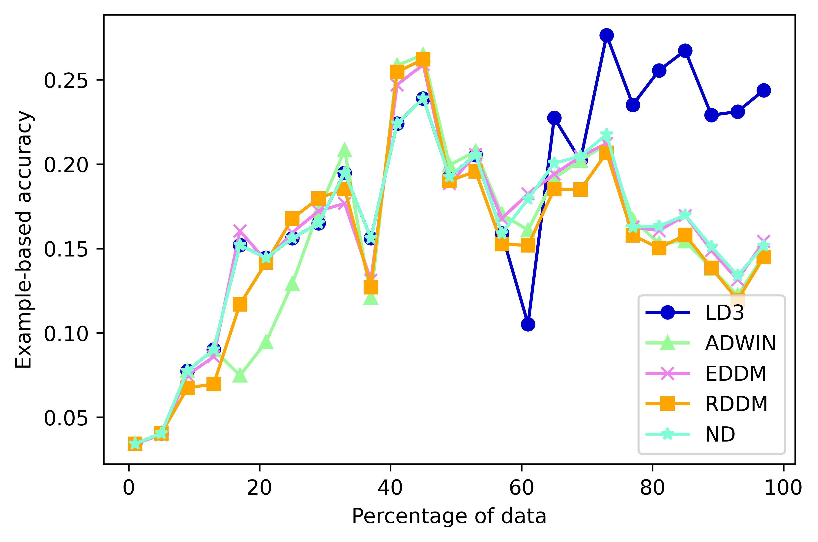
(a) Enron

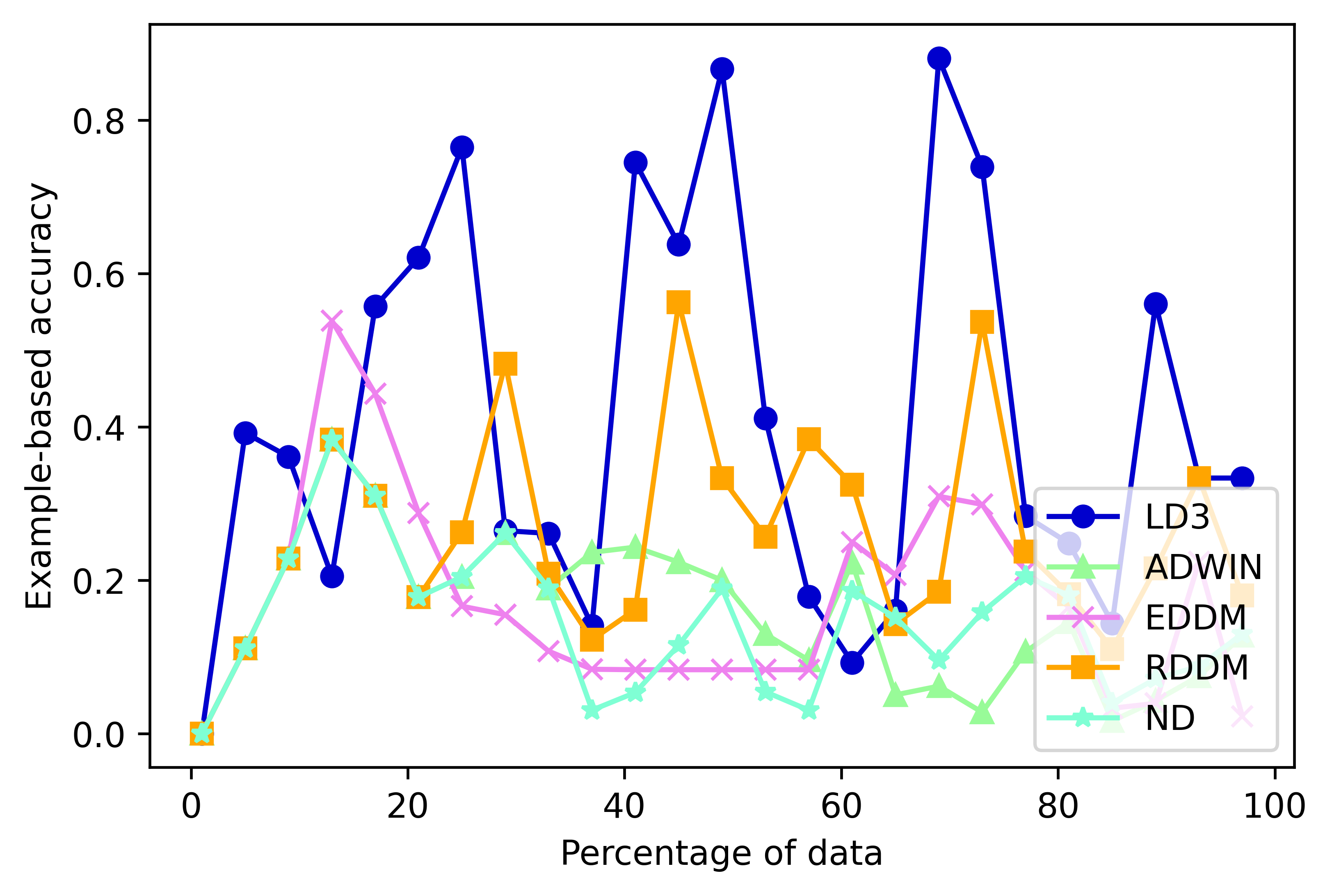
(b) PlantPseAAC

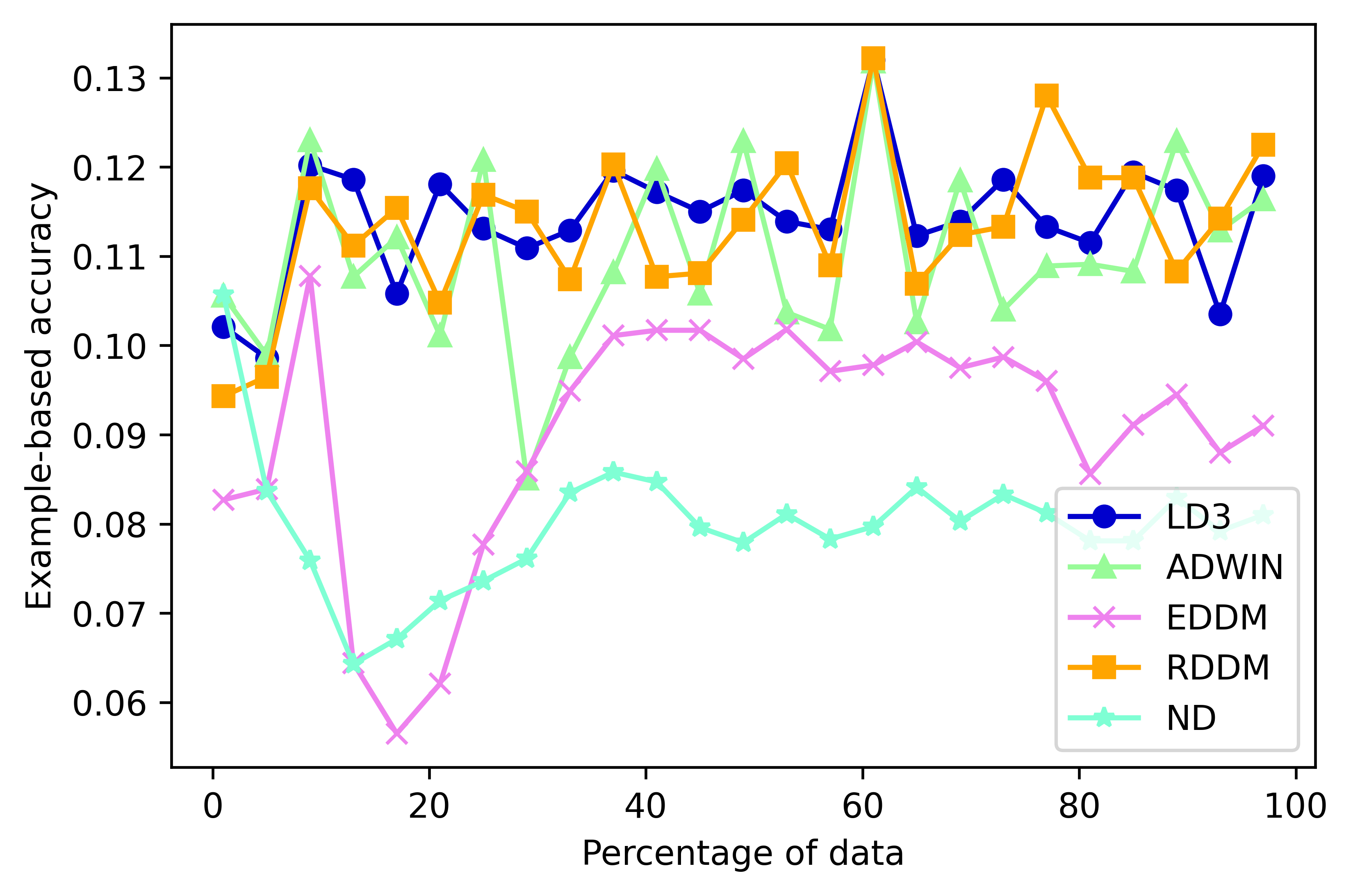
(c) Imdb

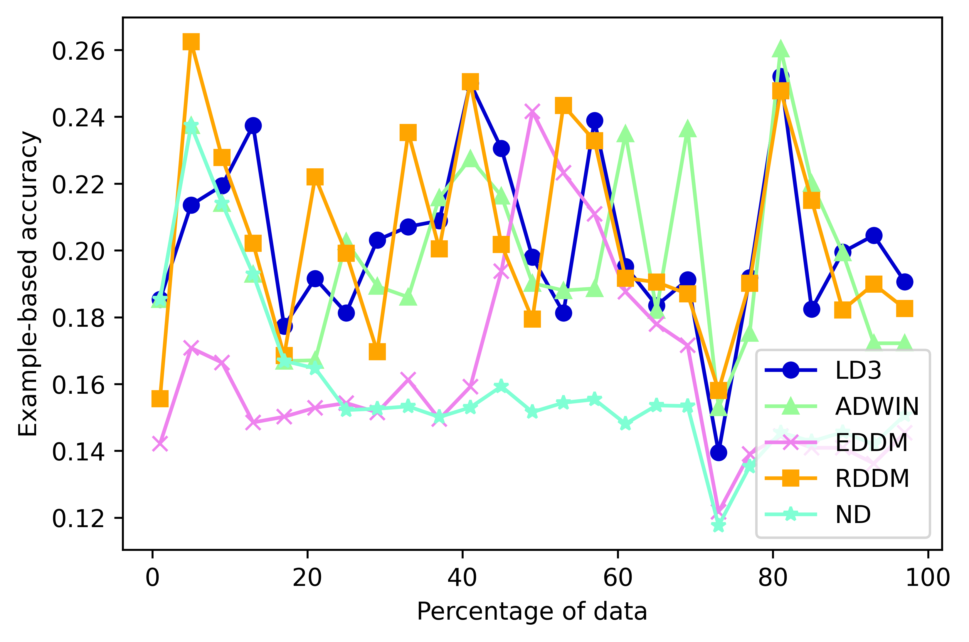
(d) Tmc2007-500

Figure 6: Example-based accuracy results of the top detectors and ND on four datasets. Y-axis of the plots is given with different scales.

It should be observed that contrary to prior expectation, ND does not show the worst results and it achieves better results compared to more than half of the tested detectors. Our experiments show that apart from ADWIN, EDDM, HDDM_A, and RDDM, the baseline detectors either do not detect drift or perform worse than ND in general. We identify the reason behind this as frequent false positive drift detections. An incorrectly detected drift leads the classifier to discard the progress it made which severely reduces the effectiveness results. In addition, after a reset, the error rate of the classifier is increased which causes an error rate-based detector to miss-interpret the miss-classification statistics and may result in oscillating drift detections. The positive feedback loop generated from both of these factors causes the detectors to produce worse results than ND.

However, our experiments confirm that ADWIN, EDDM, HDDM_A, and RDDM are suitable for drift detection on multi-label data streams. For the following discussions, we use the top four detectors in terms of average rank, namely, LD3, ADWIN, EDDM, and RDDM.

6.1.3 Time Change Analysis of Effectiveness

One aspect we would like to highlight is LD3’s ability to detect drifts even when tested with a dataset that has low label cardinality. Our initial assumption was that LD3 would perform worse on datasets with lower label cardinality, since there would be less co-occurrence. However, in datasets with low label cardinality such as Birds, 20NG, and PlantPseAAC; LD3 still outperforms the baselines in general. We found that even if the label cardinality is low, as long as the data stream is a multi-label stream, some labels still have more influence over other labels and LD3 continues to be effective. One problem that arises from this is that how the algorithm should respond if the nature of the stream changes from multi-label to multi-class stream. Our suggestion in such a case would be to switch to a different detector suited to multi-class streams since LD3 would lose its ability to detect drifts. However, we were unable to find any detectors that could detect a change in the data stream’s nature and recommend further research for such cases.

Figure 6 plots the time scale example-based accuracy results of the top four detectors and ND. These datasets are chosen as most of the detectors co-detect drifts and their plots are more clear, allowing better inspection. The datasets are divided into 25 subsets and the average accuracy within those subsets is plotted.

Most of the sudden decreases in accuracy are caused by the classifier resets which means that at those points, the algorithms deduce that drift is present. Noticeably on the PlantPseAAC dataset, the sudden decreases in accuracy occur earlier for LD3, after which the classifier produces higher accuracy values than the baselines. LD3’s early detections allow the classifier to learn larger amounts of samples and adapt to the new concept faster. This is also observed in the second half of the Enron dataset where the other detectors stagnate in accuracy while LD3 resets to learn the new drift.

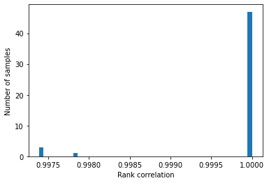
(a) EukaryotePseAAC with $t=2$

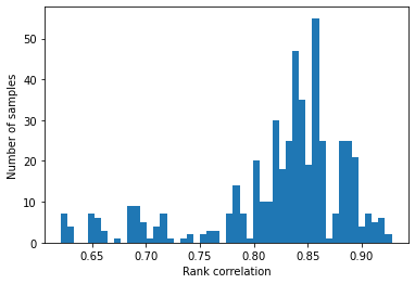
(b) Synthetic Sudden with $t=3$

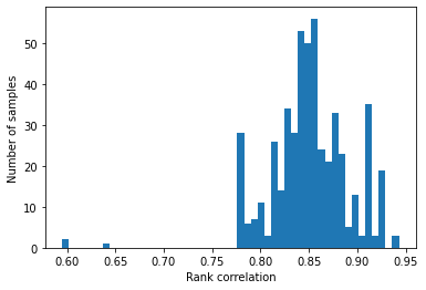
(c) Tmc2007-500 with $t=4$

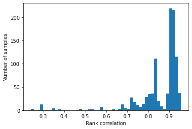
(d) 20NG with $t=5$

Figure 7: Distribution of the rank correlations within $W_{corr}$ of four datasets after a drift is detected with different $t$ values ($\sigma$ multipliers). X-axis of the plots is given with different scales.

Furthermore, the plots illustrate that LD3 is more resistant to the noisy data originating from a recently reset classifier. Notably with ADWIN and RDDM on Tmc2007-500 and Imdb datasets, we observe that there are numerous consecutive drops in accuracy, which is the result of a new detection following a recent reset. While the classifier builds a probabilistic model for the new distribution, some noise is usually expected. Yet for error rate-based algorithms like ADWIN and RDDM, this noise causes false detections that result in oscillating resets as previously discussed. LD3 combats this problem by waiting until sufficient statistics are obtained while the windows get filled, which allows faster recovery. For instance, in the Tmc2007-500 dataset, RDDM generally reaches higher accuracy values. However, RDDM resets the classifier frequently as opposed to LD3’s more stable execution, which results in marginally worse overall accuracy (LD3: 0.2029, RDDM: 0.2016) for RDDM, despite having multiple higher local maximum values. A similar case is also displayed with the Imdb dataset.

We define robustness, in the context of concept drift detection, as the ability to aid classifiers to provide the best predictive performance within a data stream with changing concepts. Our investigation on Figure 6 and results on Table 2 demonstrate that LD3 is a robust detection algorithm that assists the classifier to achieve the best effectiveness results overall, within varying streaming environments with drift.

6.1.4 Efficiency Concerns and Advantages of Unsupervised Detection

In our study, we chose not to include an efficiency analysis, because, in our experiments, we observe that a drift detector’s influence on the execution time is much lower than the paired classifier. Furthermore, supervised detection algorithms assume that the true labels are readily available (Sethi and Kantardzic, 2017; Žliobaite, 2010); however, that is not always the case in real life. The acquisition of labeled data is usually difficult and it is much easier to collect unlabeled data (Subhashini et al, 2021). As LD3 is an unsupervised detector, the lack of labeled data does not prevent its continuous concept drift detection whereas supervised algorithms may halt while waiting for labels.

6.2 Hyperparameter Analysis

In our analysis of the hyperparameters, we propose a method to set the standard deviation multiplier $t$. Furthermore, we conduct experiments to determine the effect of window size $w$ and threshold for the number of anomaly $L$.

6.2.1 Setting the Standard Deviation Multiplier $t$

We developed a simple way to tune the $t$ parameter of LD3. Figure 7 plots the distribution of past correlations within $W_{corr}$, when a drift is detected for four datasets as histogram plots.

Since LD3 is an unsupervised detector, such plots could easily be obtained as a part of the test runs of a given data stream. In the figure, we see that with each subplot the range of correlation values expand; however the mean correlation does not decrease at the same rate, where they stay in $[0.80,1]$. If the standard deviation of the correlations are very small, e.g, EukaryotePseAAC dataset in Figure 7.a, a low $t$ is required such as $t=2$. With this $t$ value, if the current correlation value is smaller than $\mu-2\sigma$, it lies outside of the 95% confidence interval and it should be considered as an anomaly (Pukelsheim, 1994). For an accurate tuning of LD3, starting from $t=2$, the confidence interval should be expanded with an increasing $t$, with guidance from the plots generated, similar to the examples in Figure 7. We used this method to determine the $t$ values for our experiments on Table 2. Among the parameter values we used, $t=4$ most frequently achieves the best effectiveness result. Therefore, we use this value as a default parameter.

6.2.2 Setting the Parameters Window Size $w$ and Threshold for Number of Anomalies $L$

To investigate the effect of $L$ and $w$ parameters, we conducted experiments on the real-world datasets using $w=[50,250,500]$, $L=[0,1,2]$ values. Table 6 presents the results of our experiments. We found that $L=0$ is a good default value since most of the best results are achieved with this value. This indicates that our concerns about outlier resiliency are not as significant as initially assumed. Though this is most likely not the case for every data stream as streams with extreme noise may be susceptible to outliers. We urge researchers who would utilize LD3 to better tune the $L$ parameter if there are available resources such as labeled data and computational capacity.

Table 6: Example-based accuracy of LD3 with varying parameter settings for each real-world dataset The best scores are highlighted in bold. Datasets are listed in ascending order of the number of data items they contain.

Dataset	$N$	$w=50$ $L=0$	$w=50$ $L=1$	$w=50$ $L=2$	$w=250$ $L=0$	$w=250$ $L=1$	$w=250$ $L=2$	$w=500$ $L=0$	$w=500$ $L=1$	$w=500$ $L=2$
Birds	645	0.0618	0.0550	0.0550	0.0550	0.0550	0.0550	0.0550	0.0550	0.0550
PlantPseAAC	978	0.1383	0.1369	0.1369	0.1369	0.1369	0.1369	0.1369	0.1369	0.1369
Enron	1,702	0.1055	0.1089	0.1371	0.1403	0.1301	0.1371	0.1371	0.1371	0.1371
Yeast	2,417	0.3780	0.3644	0.3622	0.3724	0.3720	0.3718	0.3613	0.3613	0.3613
EukaryotePseAAC	7,766	0.1663	0.0727	0.0327	0.0627	0.0647	0.0658	0.0587	0.0578	0.0593
Ohsumed	13,930	0.0367	0.0370	0.0608	0.0444	0.0443	0.0443	0.0630	0.0630	0.0527
20NG	19,300	0.0667	0.0733	0.1469	0.1209	0.1219	0.1247	0.1516	0.1384	0.1497
Tmc2007-500	28,600	0.1485	0.1918	0.1555	0.1931	0.1934	0.1980	0.2029	0.2009	0.2007
Imdb	120,900	0.0717	0.0810	0.0797	0.0950	0.0954	0.1012	0.1129	0.1124	0.1140

Unlike the $L$ parameter, our results show that setting the $w$ parameter to a default value is not as straightforward. In Table 6 we observe that the datasets with low number of samples performs best with $w=50$ and larger datasets with $w=500$. This is related to the problem of sampling rate for data streams. Depending on the problem domain, the source of a stream can be sampled daily for stable streams such as music billboard charts and it can be sampled several times a minute for volatile data streams such as the price of a cryptocurrency. For this purpose it is possible to use a hyperparameter self-tuning scheme (Veloso et al, 2021), to better adjust the classifier based on the current distribution. In our experiments, we observe that the value of the $w$ parameter is highly dependant on the sampling rate of a stream and it should be set accordingly. For frequently sampled data streams we recommend $w=500$ as a default value and $w=50$ for infrequently sampled streams.

6.3 Analysis of Different Fusion Methods

In order to study the effects of different data fusion algorithms and to choose a suitable, default data fusion algorithm for LD3, we conducted experiments on the nine real-world datasets we used on effectiveness tests. We chose to exclude the synthetic data streams for these experiments as we aim to evaluate the general effectiveness of the tested data fusion algorithms in real-world datasets. In these experiments, in addition to reciprocal ranking, we used popular data fusion algorithms Borda Fuse, Condorcet’s Fuse (Nuray and Can, 2006) and Markov Chains Type 4 (MC4) (Dwork et al, 2001). The results are shown in Table 7. The tests are done by only changing the data fusion section of LD3.

Table 7: Example-based accuracy results of LD3 using four different data fusion algorithms. Best results are highlighted in bold.

Dataset	Reciprocal	Borda	Condorcet	MC4
20NG	0.1616	0.1480	0.1497	0.1517
Birds	0.0992	0.0913	0.0984	0.0903
Enron	0.1403	0.1343	0.1316	0.1368
EukaryotePseAAC	0.1946	0.2096	0.0727	0.0685
Imdb	0.1140	0.1154	0.1110	0.1134
Ohsumed	0.0693	0.0568	0.0595	0.0594
PlantPseAAC	0.3198	0.3393	0.2397	0.2099
Tmc2007-500	0.2029	0.1954	0.1999	0.1997
Yeast	0.3765	0.3643	0.3577	0.3586

The results show that reciprocal rank fusion provides better results (in six of the nine cases). This is within our expectations as past studies such as Cormack et al (2009) and Pedronette and Torres (2015) have shown similar observations in different problem domains.

6.4 Influence of Drift Types and Speed

Regarding drift types, since LD3 counts the number of co-occurrences to detect concept drift, incremental, sudden, and reoccurring drifts have the same structure as all of these types of drift result in changing rankings. As shown in Table 2, LD3 generally performs the same between different types of drifts and outperforms other detectors. Also, from the algorithm perspective, both incremental and gradual drifts show the same structure within the co-occurrence matrix. Therefore, we chose not to add an additional stream for gradual drift as the results were very similar.

Table 8: Example-based accuracy results of the top detectors with different drift types. Best results are highlighted in bold.

Data Stream	LD3	ADWIN	EDDM	RDDM	ND
Sudden_1	0.0788	0.0724	0.0744	0.0720	0.0659
Sudden_25	0.0767	0.0724	0.0741	0.0724	0.0659
Sudden_50	0.0776	0.0725	0.0737	0.0724	0.0659
Incremental_250	0.0769	0.0725	0.0733	0.0731	0.0659
Incremental_500	0.0788	0.0724	0.0787	0.0722	0.0659
Incremental_1000	0.0776	0.0717	0.0766	0.0713	0.0659

In addition to drift types, the speed at which the drift occurs also influences a detector’s ability to find drifts. In Table 8, the accuracy results of the top four detectors are presented. The streams used are synthetic data streams with sudden and incremental drifts and the number after the underscore is the number of samples over which the drift occurs. We generate them using the Scikit-Multiflow framework (Montiel et al, 2018) by the same method described in Section 5.1 where they have 20,000 samples, 50 classes, and 200 features with drifts occurring at sample positions 4,000 and 10,000. Our findings indicate that regardless of the drift speed and type, LD3 still outperforms the baseline detectors, which demonstrate LD3’s robustness under different speed conditions.

7 Conclusion

In this paper, we present LD3, a novel unsupervised concept drift detection algorithm that exploits dynamic temporal dependencies between class labels in a multi-label classification environment. The algorithm is based on a new concept, label dependency ranking, which we introduce. We perform an extensive evaluation of LD3 against 14 prevalent drift detection algorithms using a Classifier Chain of Gaussian Naive Bayes classifiers. The experimental results show that LD3 provides the highest classifier accuracy: Without using true class labels, it statistically significantly outperforms several of the other drift detection algorithms that require such labels.

Our algorithm is able to accurately assist multi-label classifiers in the presence of a concept drift, which results in more robust classification models that are more adaptive to changing trends. In many streaming environments, true class labels required by supervised concept drift detection methods are likely to be unavailable due to several reasons. As LD3 is an unsupervised algorithm, this advantage illustrates the practical value of LD3.

In future work, we plan to examine the uses of LD3 in unsupervised classification and in environments that include concept evolution, i.e. the emergence of entirely new labels.

Appendix A Detailed Calculation Example

Assume that a given data stream $S_{0,t}={d_{0},...,d_{t}}$, in a time window $[0,t]$, where $d_{i}=(X_{i},y_{i})$, the window size $w=3$ and three classes, the most recent six predictions are:

$$S=((0,0,1),(1,1,1),(0,1,1),\mathbf{(1,0,1),(1,1,0),(1,0,1))}$$ (9)

We first calculate two co-occurrence matrices $M_{new}$ and $M_{old}$. For $M_{new}$ we use the most recent $w$ labels which are highlighted in bold. The next $w$ labels after that are used for $M_{old}$. The matrices are calculated by counting the number of times each label occurs together. For instance, for the third sample $(0,1,1)$, the second and third labels are true together, so $M_{old}(2,3)$ and $M_{old}(3,2)$ are incremented by one. Each row of the matrices represents the co-occurrence for a different label. For the given stream, the resulting matrices are the following:

$$\begin{aligned} M_{old}=\begin{bmatrix}0&\quad 1&\quad 1\\ 1&\quad 0&\quad 2\\ 1&\quad 2&\quad 0\end{bmatrix}\end{aligned}\qquad\qquad\qquad\qquad\qquad\qquad\qquad\qquad\begin{aligned} M_{new}=\begin{bmatrix}0&\quad 1&\quad 2\\ 1&\quad 0&\quad 0\\ 2&\quad 0&\quad 0\end{bmatrix}\end{aligned}$$ (A2)

Next, we calculate the ranking of the co-occurrences for each label, i.e, which labels occur more frequently together with the currently ranked label. A.4 is for $M_{old}$ and A.5 is for $M_{new}$, where $L_{i}$ represents the rankings for each past predicted label and $L^{\prime}_{i}$ is used for the most recently predicted labels.

$$\begin{aligned} \hfil\displaystyle\begin{split}L_{1}\leftarrow l_{2}=l_{3}\\ L_{2}\leftarrow l_{3}>l_{1}\\ L_{3}\leftarrow l_{2}>l_{1}\end{split}\end{aligned}\qquad\qquad\qquad\qquad\qquad\qquad\qquad\qquad\begin{aligned} \hfil\displaystyle\begin{split}L^{\prime}_{1}\leftarrow l_{3}>l_{2}\\ L^{\prime}_{2}\leftarrow l_{1}>l_{3}\\ L^{\prime}_{3}\leftarrow l_{1}>l_{2}\end{split}\end{aligned}$$ (A3)

We perform reciprocal rank fusion on the obtained rankings to get a global, aggregated ranking for the old and new labels. For tied rankings, we assume they each have the same ranking. $r_{i}$ and $r^{\prime}_{i}$ are the reciprocal rank of each label for old and new predictions in their respective order. The calculated ranks are sorted in ascending order to get the global rankings $R_{old}$ and $R_{new}$. If two reciprocal ranks are equal, they are sorted based on their label indexes.

$$\begin{aligned} \hfil\displaystyle\begin{split}r_{1}=\frac{1}{\frac{1}{2}+\frac{1}{2}}=1\\ r_{2}=\frac{1}{\frac{1}{1}+\frac{1}{1}}=\frac{1}{2}\\ r_{3}=\frac{1}{\frac{1}{1}+\frac{1}{1}}=\frac{1}{2}\\ \\ R_{old}=[l_{2},l_{3},l_{1}]\end{split}\end{aligned}\qquad\qquad\qquad\qquad\qquad\qquad\qquad\qquad\begin{aligned} \hfil\displaystyle\begin{split}r^{\prime}_{1}=\frac{1}{\frac{1}{1}+\frac{1}{1}}=\frac{1}{2}\\ r^{\prime}_{2}=\frac{1}{\frac{1}{2}+\frac{1}{2}}=1\\ r^{\prime}_{3}=\frac{1}{\frac{1}{1}+\frac{1}{2}}=\frac{2}{3}\\ \\ R_{new}=[l_{1},l_{3},l_{2}]\end{split}\end{aligned}$$ (A4)

The obtained $R_{old}$ and $R_{new}$ rankings are then used to calculate the WS coefficient to measure the rank correlation between the two rankings. In A.8, the ranks represent the ranking position of the i-th label where $R^{old}=[2,0,1]$ and $R^{new}=[0,2,1]$.

$$C=1-\sum_{i=1}^{3}\bigg{(}2^{-R^{new}_{i}}\cdot\frac{|R^{new}_{i}-R^{old}_{i}|}{max\{|1-R^{new}_{i}|,|3-R^{new}_{i}|\}}\bigg{)}$$ (A5)

$$\begin{split}C=1-\bigg{(}2^{0}\cdot\frac{|0-2|}{max\{|1-0|,|3-0|\}}+2^{-2}\cdot\frac{|2-0|}{max\{|1-2|,|3-2|\}}+\\ 2^{-1}\cdot\frac{|1-1|}{max\{|1-1|,|3-1|\}}\bigg{)}\end{split}$$ (A6)

$$C=1-\bigg{(}\frac{2}{3}+\frac{1}{2}+0\bigg{)}=-0.167$$ (A7)

For the remaining part, if the obtained correlation $C$ is less than $\mu-t\sigma$, where $\mu$ is the mean, $\sigma$ is the standard deviation and $t$ is the $\sigma$ multiplier used in three sigma rule, the obtained correlation is added to an anomaly list. The drift is detected when the length of the anomaly list generated from $W_{corr}$ is greater than the set $L$ threshold.

References

- \bibcommenthead
- Baena-Garcıa et al (2006) Baena-Garcıa M, del Campo-Ávila J, Fidalgo R, et al (2006) Early drift detection method. In: Fourth International Workshop on Knowledge Discovery from Data Streams, pp 77–86
- Bahri et al (2021) Bahri M, Bifet A, Gama J, et al (2021) Data stream analysis: Foundations, major tasks and tools. Wiley Interdisciplinary Reviews: Data Mining and Knowledge Discovery 11(3):e1405
- Barros et al (2017) Barros RS, Cabral DR, Gonçalves Jr PM, et al (2017) Rddm: Reactive drift detection method. Expert Systems with Applications 90:344–355
- Bifet and Gavalda (2007) Bifet A, Gavalda R (2007) Learning from time-changing data with adaptive windowing. In: Proceedings of the 2007 SIAM International Conference on Data Mining, SIAM, pp 443–448
- Bonab and Can (2018) Bonab HR, Can F (2018) GOOWE: Geometrically optimum and online-weighted ensemble classifier for evolving data streams. ACM Transactions on Knowledge Discovery from Data (TKDD) 12(2):1–33
- Büyükçakir et al (2018) Büyükçakir A, Bonab H, Can F (2018) A novel online stacked ensemble for multi-label stream classification. In: Proceedings of the 27th ACM International Conference on Information and Knowledge Management, pp 1063–1072
- Cormack et al (2009) Cormack GV, Clarke CL, Buettcher S (2009) Reciprocal rank fusion outperforms condorcet and individual rank learning methods. In: Proceedings of the 32nd International ACM SIGIR Conference on Research and Development in Information Retrieval, pp 758–759
- Demšar (2006) Demšar J (2006) Statistical comparisons of classifiers over multiple data sets. Journal of Machine Learning Research 7(Jan):1–30
- Dwork et al (2001) Dwork C, Kumar R, Naor M, et al (2001) Rank aggregation methods for the web. In: Proceedings of the 10th International Conference on World Wide Web, pp 613–622
- Frías-Blanco et al (2014) Frías-Blanco I, del Campo-Ávila J, Ramos-Jimenez G, et al (2014) Online and non-parametric drift detection methods based on hoeffding’s bounds. IEEE Transactions on Knowledge and Data Engineering 27(3):810–823
- Gama et al (2004) Gama J, Medas P, Castillo G, et al (2004) Learning with drift detection. In: Brazilian Symposium on Artificial Intelligence, Springer, pp 286–295
- Gama et al (2009) Gama J, Sebastião R, Rodrigues PP (2009) Issues in evaluation of stream learning algorithms. In: Proceedings of the 15th ACM SIGKDD International Conference on Knowledge Discovery and Data Mining, pp 329–338
- Gama et al (2014) Gama J, Žliobaitė I, Bifet A, et al (2014) A survey on concept drift adaptation. ACM Computing Surveys (CSUR) 46(4):1–37
- Gemaque et al (2020) Gemaque RN, Costa AFJ, Giusti R, et al (2020) An overview of unsupervised drift detection methods. Wiley Interdisciplinary Reviews: Data Mining and Knowledge Discovery 10(6):e1381
- Gözüaçık and Can (2021) Gözüaçık Ö, Can F (2021) Concept learning using one-class classifiers for implicit drift detection in evolving data streams. Artificial Intelligence Review 54(5):3725–3747
- Gözüaçık et al (2019) Gözüaçık Ö, Büyükçakır A, Bonab H, et al (2019) Unsupervised concept drift detection with a discriminative classifier. In: Proceedings of the 28th ACM International Conference on Information and Knowledge Management, pp 2365–2368
- Guo and Gu (2011) Guo Y, Gu S (2011) Multi-label classification using conditional dependency networks. In: Twenty-Second International Joint Conference on Artificial Intelligence
- Hammami et al (2020) Hammami Z, Sayed-Mouchaweh M, Mouelhi W, et al (2020) Neural networks for online learning of non-stationary data streams: a review and application for smart grids flexibility improvement. Artificial Intelligence Review 53:6111–6154
- Hoeffding (1963) Hoeffding W (1963) Probability inequalities for sums of bounded random variables. Journal of the American Statistical Association 58(301):13–30. 10.1080/01621459.1963.10500830
- Iwashita and Papa (2018) Iwashita AS, Papa JP (2018) An overview on concept drift learning. Ieee Access 7:1532–1547
- John (1995) John G (1995) Estimating continuous distributions in bayesian classifiers. In: Proc. 11th Conference on Uncertainty in Artificial Intelligence
- Kendall (1938) Kendall MG (1938) A new measure of rank correlation. Biometrika 30(1/2):81–93
- Koh (2016) Koh YS (2016) Cd-tds: Change detection in transactional data streams for frequent pattern mining. In: 2016 International Joint Conference on Neural Networks (IJCNN), IEEE, pp 1554–1561
- Lu et al (2018) Lu J, Liu A, Dong F, et al (2018) Learning under concept drift: A review. IEEE Transactions on Knowledge and Data Engineering 31(12):2346–2363
- de Mello et al (2019) de Mello RF, Vaz Y, Grossi CH, et al (2019) On learning guarantees to unsupervised concept drift detection on data streams. Expert Systems with Applications 117:90–102
- Montiel et al (2018) Montiel J, Read J, Bifet A, et al (2018) Scikit-multiflow: A multi-output streaming framework. The Journal of Machine Learning Research 19(1):2915–2914
- Nam et al (2017) Nam J, Mencía EL, Kim HJ, et al (2017) Maximizing subset accuracy with recurrent neural networks in multi-label classification. In: Proceedings of the 31st International Conference on Neural Information Processing Systems, pp 5419–5429
- Nuray and Can (2006) Nuray R, Can F (2006) Automatic ranking of information retrieval systems using data fusion. Information Processing & Management 42(3):595–614
- Pears et al (2014) Pears R, Sakthithasan S, Koh YS (2014) Detecting concept change in dynamic data streams. Machine Learning 97(3):259–293
- Pedronette and Torres (2015) Pedronette DCG, Torres RdS (2015) Unsupervised effectiveness estimation for image retrieval using reciprocal rank information. In: 2015 28th SIBGRAPI Conference on Graphics, Patterns and Images, IEEE, pp 321–328
- Pesaranghader and Viktor (2016) Pesaranghader A, Viktor HL (2016) Fast hoeffding drift detection method for evolving data streams. In: Joint European Conference on Machine Learning and Knowledge Discovery in Databases, Springer, pp 96–111
- Pesaranghader et al (2018a) Pesaranghader A, Viktor H, Paquet E (2018a) Reservoir of diverse adaptive learners and stacking fast hoeffding drift detection methods for evolving data streams. Machine Learning 107(11):1711–1743
- Pesaranghader et al (2018b) Pesaranghader A, Viktor HL, Paquet E (2018b) Mcdiarmid drift detection methods for evolving data streams. In: 2018 International Joint Conference on Neural Networks (IJCNN), IEEE, pp 1–9
- Pinagé et al (2020) Pinagé F, dos Santos EM, Gama J (2020) A drift detection method based on dynamic classifier selection. Data Mining and Knowledge Discovery 34(1):50–74
- Pintas et al (2021) Pintas JT, Fernandes LA, Garcia ACB (2021) Feature selection methods for text classification: a systematic literature review. Artificial Intelligence Review pp 1–52
- Pukelsheim (1994) Pukelsheim F (1994) The three sigma rule. The American Statistician 48(2):88–91
- Raab et al (2020) Raab C, Heusinger M, Schleif FM (2020) Reactive soft prototype computing for concept drift streams. Neurocomputing
- Read et al (2011) Read J, Pfahringer B, Holmes G, et al (2011) Classifier chains for multi-label classification. Machine Learning 85(3):333
- Read et al (2016) Read J, Reutemann P, Pfahringer B, et al (2016) Meka: a multi-label/multi-target extension to weka. The Journal of Machine Learning Research 17(1):667–671
- dos Reis et al (2016) dos Reis DM, Flach P, Matwin S, et al (2016) Fast unsupervised online drift detection using incremental kolmogorov-smirnov test. In: Proceedings of the 22nd ACM SIGKDD International Conference on Knowledge Discovery and Data Mining, pp 1545–1554
- Roseberry and Cano (2018) Roseberry M, Cano A (2018) Multi-label knn classifier with self adjusting memory for drifting data streams. In: Second International Workshop on Learning with Imbalanced Domains: Theory and Applications, PMLR, pp 23–37
- Sałabun and Urbaniak (2020) Sałabun W, Urbaniak K (2020) A new coefficient of rankings similarity in decision-making problems. In: International Conference on Computational Science, Springer, pp 632–645
- Sethi and Kantardzic (2017) Sethi TS, Kantardzic M (2017) On the reliable detection of concept drift from streaming unlabeled data. Expert Systems with Applications 82:77–99
- Shi et al (2014) Shi Z, Wen Y, Feng C, et al (2014) Drift detection for multi-label data streams based on label grouping and entropy. In: 2014 IEEE International Conference on Data Mining Workshop, IEEE, pp 724–731
- Spearman (1987) Spearman C (1987) The proof and measurement of association between two things. The American Journal of Psychology 100(3/4):441–471
- Subhashini et al (2021) Subhashini L, Li Y, Zhang J, et al (2021) Mining and classifying customer reviews: a survey. Artificial Intelligence Review pp 1–47
- Tsoumakas and Katakis (2007) Tsoumakas G, Katakis I (2007) Multi-label classification: An overview. International Journal of Data Warehousing and Mining (IJDWM) 3(3):1–13
- Veloso et al (2021) Veloso B, Gama J, Malheiro B, et al (2021) Hyperparameter self-tuning for data streams. Information Fusion 76:75–86
- Vigna (2015) Vigna S (2015) A weighted correlation index for rankings with ties. In: Proceedings of the 24th International Conference on World Wide Web, pp 1166–1176
- Wang and Zhang (2020) Wang D, Zhang S (2020) Unsupervised person re-identification via multi-label classification. In: Proceedings of the IEEE/CVF Conference on Computer Vision and Pattern Recognition (CVPR)
- Wang et al (2016) Wang J, Yang Y, Mao J, et al (2016) Cnn-rnn: A unified framework for multi-label image classification. In: Proceedings of the IEEE Conference on Computer Vision and Pattern Recognition, pp 2285–2294
- Wang et al (2020) Wang P, Jin N, Fehringer G (2020) Concept drift detection with false positive rate for multi-label classification in iot data stream. In: 2020 International Conference on UK-China Emerging Technologies (UCET), IEEE, pp 1–4
- Xu et al (2019) Xu D, Shi Y, Tsang IW, et al (2019) Survey on multi-output learning. IEEE Transactions on Neural Networks and Learning Systems
- Xue et al (2011) Xue X, Zhang W, Zhang J, et al (2011) Correlative multi-label multi-instance image annotation. In: 2011 International Conference on Computer Vision, IEEE, pp 651–658
- Zhang and Zhang (2010) Zhang ML, Zhang K (2010) Multi-label learning by exploiting label dependency. In: Proceedings of the 16th ACM SIGKDD International Conference on Knowledge Discovery and Data Mining, pp 999–1008
- Zhang and Zhou (2013) Zhang ML, Zhou ZH (2013) A review on multi-label learning algorithms. IEEE Transactions on Knowledge and Data Engineering 26(8):1819–1837
- Zheng et al (2019) Zheng X, Li P, Chu Z, et al (2019) A survey on multi-label data stream classification. IEEE Access
- Žliobaite (2010) Žliobaite I (2010) Change with delayed labeling: When is it detectable? In: 2010 IEEE International Conference on Data Mining Workshops, IEEE, pp 843–850