AutoGeoLabel:
Automated Label Generation
for Geospatial Machine Learning

Abstract

A key challenge of supervised learning is the availability of human-labeled data. We evaluate a big data processing pipeline to auto-generate labels for remote sensing data. It is based on rasterized statistical features extracted from surveys such as e.g. LiDAR measurements. Using simple combinations of the rasterized statistical layers, it is demonstrated that multiple classes can be generated at accuracies of $\sim 0.9$.
As proof of concept, we utilize the big geo-data platform IBM PAIRS to dynamically generate such labels in dense urban areas with multiple land cover classes. The general method proposed here is platform independent, and it can be adapted to generate labels for other satellite modalities in order to enable machine learning on overhead imagery for land use classification and object detection.

I Introduction & Motivation

Driven by the availability of massive amounts of data, image classification achieves accuracy of over 90% with thousands of classes, today [1]. To a large extent, the performance of modern deep learning models is driven by the volume of data, and the availability of accurate labels for training. Popular datasets such as ImageNet [2], COCO [3], and MNIST [4] serve as benchmarks for assessing machine learning model performance. These benchmarks were generated by visual inspection of images to manually craft labels. Extension to new labels or classes requires additional effort. The same procedure—as previously executed for the collection of existing labels—needs application to the new, unlabeled set of data.

While image classification achieved tremendous success for photographs, a straightforward adoption of established machine learning techniques for satellites, drones, and remote sensing images have limited success [5, 6, 7, 8]. In general, geospatial image classification [9] lags behind machine learning precision from social media [10]—due to more sparsely labeled data, and due to increased heterogeneity in data.

Remote sensing signals often demand far more sophisticated processing compared with conventional photography. For instance, Light Detection and Ranging (LiDAR) [11]—acquired as a 3D point cloud—requires processing and conversion of the data into a commonly usable machine learning 2D data input format; such as a multi-dimensional array of numbers [12, 13]. Geospatial data also come with varying spatial resolution acquired across multiple seasons. Real time integration of satellite data into multidimensional models like weather or climate requires automation of label generation. For example: Identification of extreme weather events such as a hurricane, earthquakes, wildfires, etc., demands specific training data with need to generate labels on the fly as those events are forming.

Here we propose AutoGeoLabel, a framework to create labels for geospatial imagery. It extracts features using simple statistical methods from raw and unlabeled data. The approach allows to identify class labels from a combination of rasterized layers. We demonstrate the utility of such an approach taking LiDAR measurements to exemplify how simple combinations of statistical features can help to automatically classify a geospatial scene. As a result, such rapidly generated labels may get exploited to identify land cover as (noisy) input for machine learning models.

The framework is developed to label large volumes of data, and to create labels in near real time for any image type. Moreover, the method is not limited to LiDAR, but may get adopted for any other high quality data available for the area of interest such as hyper- and multi-spectral imaging, synthetic aperture radar (SAR), or microwave radiometry.

II Previous Work & Applications

Labeled geospatial data for machine learning benchmarks is hard to come by, and those is sensor platform specific. Commonly, labels from land classification is typically rooted in a combination of pixel- and object-based classifications [14]. Generated land cover data is often corrected through a data quality process where manual reclassification is carried out. Additional maps and land use datasets may get exploited in the process. Given the (human) effort involved in generating land cover data, those is limited in spatial coverage or temporal updates. Typical refresh rates read once in about 3–5 years [14, 15]. Standard classified data like CORINE Land Cover [14] and Multi-Resolution Land Characteristics (MRLC) [15] products have a spatial resolution of tens of meters, limited spatial coverage, and the number of classes is restricted to the most common land covers—like forest, water bodies, and agricultural lands, etc. Standard geospatial benchmark datasets like Spacenet [16], BigEarthNet [17], and DeepSat[18] have an even more limited number of labeled classes.

In contrast, OpenStreetMap (OSM) is one of the most complete, crowd-sourced community efforts with hundreds of labels collected by volunteers [19]. OSM labels is represented in vector shape format (points, lines, polygons) from which rasterized maps can get generated where roads, houses, buildings, and vegetation-covered areas is color-coded. It has been demonstrated that such OSM-based land classification labels may train deep neural network models for semantic segmentation of high-resolution, multi-spectral imagery [20]. In particular, uneven OSM-label completeness of different geographies added noise to the segmentation task. Technically, semantic segmentation was handled by unsupervised image-style translation employing a modified CycleGAN [21] architecture.

Concerning remote sensing image classification in general, standard machine learning tools previously applied read e.g. Random Forest [22], Support Vector Machine [23], XGBoost [24], and a plethora of deep learning models [25].

Geospatial data is one of the most prevalent data in Energy & Utility, Oil & Gas, Forestry, Agriculture, Transportation, Navigation, and Disaster Emergency Response [26]. Many of the above industries do have massive amounts of data collected through conventional observation, sensing, and various other measurement methods. However, the absence of labels impedes most of automation and predictive methods based on machine learning.

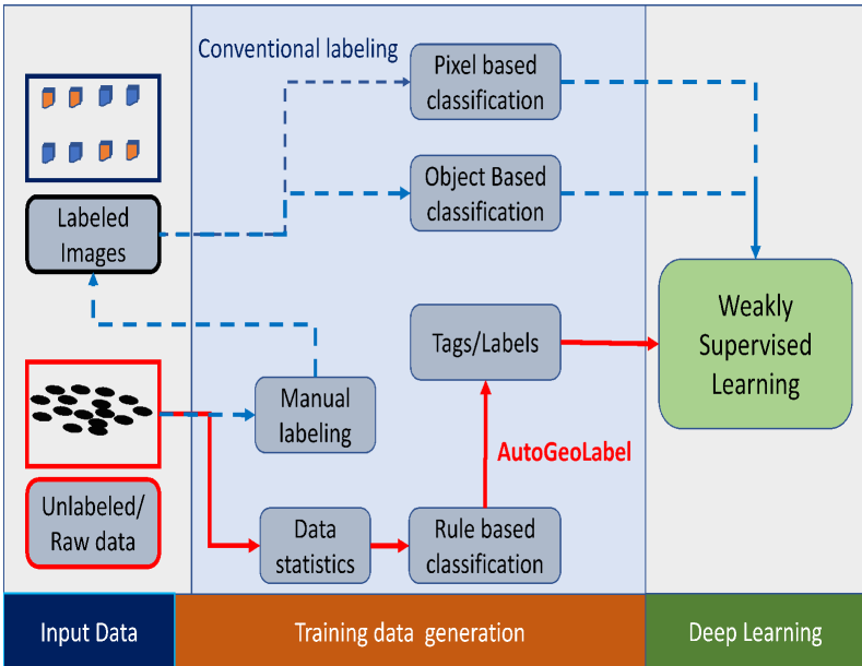
Figure 1: Schematic flow chart of the AutoGeoLabel framework to generate labeled data for machine learning. Motivated by the shortage in geospatial labels (Sec. I) where at the same time there exists vast amounts and a plurality of unstructured geospatial information (Sec. III), AutoGeoLabel automatically generates labels for weakly supervised learning.

For many industries, the large number of features of interest requires dedicated efforts to create labeled datasets based on domain expertise. AutoGeoLabel may address such situations where labels and images is generated on the fly and computational resources is limited. AutoGeoLabel bears potential for lightweight computational techniques ready for deployment on e.g. Internet-of-Things (IoT) [27] edge devices [28].

III Datasets and Geospatial Platform

III-A LiDAR Data

LiDAR data generate a dense point cloud from laser pulses bouncing back from the Earth’s surface. Massive amounts of LiDAR data is acquired mainly to map topography. In addition to elevation mapping, LiDAR carries rich embedded information on land cover such as vegetation, roads, buildings, etc. However, extracting such features may require reclassification of the point cloud, but it is prohibitively expensive. AutoGeoLabel can enable rapid label generation for existing petabytes of data [29]. For our test case, point cloud data was collected in 2017, with approx. 10 points per square meter density [30]. A small subset of point cloud data was classified into broad classes associated with water, ground, and bridges. However the majority of points fell into the unclassified category. The data volume is in excess of $1$ terabyte, and the data is made available as about $1900$ LAS 3D point cloud files [31].

III-B Land Cover Data

The LiDAR data of Sec. III-A was further processed by NYC in combination with high resolution, multi-spectral imagery to generate an $8$–class land cover dataset at $0.5$ meters resolution [32]. The $8$ classes read: Tree Canopy, Grass/Shrub, Bare Soil, Water, Buildings, Roads, Other Impervious, and Railroads. Each bears accuracy in classification above 90%. The data was also adjusted based on previous city surveys on roads, rails, and building footprints to further improve classification accuracy. We employ the Land Cover data as a ground truth validation set of AutoGeoLabel-generated classes. Such land cover classes, as obtained for NYC, is not readily available for most parts of the world. In many cases classification from the OpenStreetMap (OSM) project [19] is the best at hand.

III-C Geospatial Platforms

Open-source geospatial data volume exceeds petabytes making it comparable in volume to data generated by social media [33]. Multiple geospatial platforms exist where images are stored either as objects [34, 35, 36] or as indexed pixels ready for computation [37, 38]. IBM PAIRS does index all pixels exploiting a set of predefined spatial grids to align data layers. This approach renders ideal for search of similarities across large geographies. Also, the framework proofs efficient to apply similar processing across multiple datasets.

Current efforts to enable widespread analytics on geospatial data focus on automating machine learning [39, 40] to lower the user’s effort in creating training data, train models, and aggregate generated results. If label data is sparse or missing, AutoGeoLabel can quickly generate the required classes.

IV Methods

IV-A Feature Extraction from Point Cloud Data

Open-source earth observation data libraries such as the Geospatial Data Abstraction Library (GDAL) [41] and the Point Data Abstraction Library (PDAL) [42] enable handling and manipulation of a plurality of geospatial data formats. Python application programming interfaces (API) wrapping these libraries provide data scientists low-barrier access to G/PDAL functionalities. The libraries also offer an easy way to filter and sort information based on a set of statistical attributes. AutoGeoLabel constructs processing pipelines built on GDAL, PDAL, and Python’s NumPy module [43]: Raw point cloud data is rasterized as detailed below with the aid of PDAL. Those rasters get reprojected and aligned into a nested grid utilizing GDAL. Once curated with IBM PAIRS, fusion with other data layers such as multi-spectral imagery allows queries to pull data cubes as NumPy arrays through the PAIRS Python API wrapper (PAW) [44] for machine/deep learning consumption (cf. e.g. PyTorch tensors [12]).

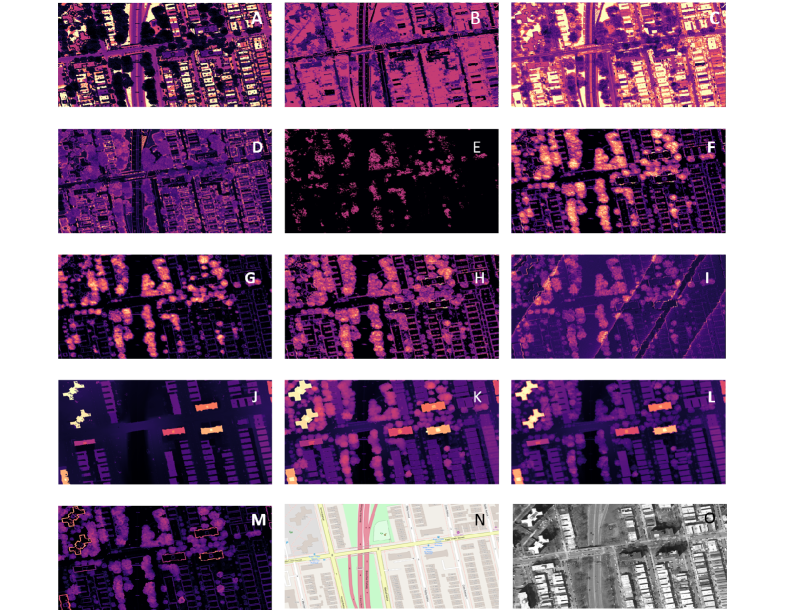
Figure 2: A–M: Statistical LiDAR features, cf. Tab. I, as extracted from the original point cloud for a sample area in NYC. Each layer is stored as individual raster grid with spatial resolution of $\sim 0.5$ meters. N: depicts OSM labels of the same area as reference; with corresponding orthophoto (O) to the right.

TABLE I: Point Cloud Statistics

attribute	statistics	Fig. 2 index
	minimum $r_{-}$	A
reflectance $r$	maximum $r_{+}$	B
	mean $\overline{r}$	C
	standard deviation $r_{\Delta}$	D
	minimum $c_{-}$	E
	maximum $c_{+}$	F
count $c$	mean $\overline{c}$	G
	standard deviation $c_{\Delta}$	H
	sum $\sum$	I
	minimum $e_{-}$	J
elevation $e$	maximum $e_{+}$	K
	mean $\overline{e}$	L
	standard deviation $e_{\Delta}$	M

For LiDAR data, attributes such as Intensity, Number of Returns, and Count is recorded to quantify the laser light reflected by the probing pulse sent from the airborne LiDAR device. While the point cloud may get automatically classified by the data provider, it typically requires specialized, commercial, and compute intensive software.

Rather than the use of proprietary data processing, in general, AutoGeoLabel employs simple statistical features extracted from high spatial resolution, high quality data. As a demonstration, here, we present the approach for LiDAR point clouds. The spatial distribution of the point cloud is determined given a local neighborhood parametrized by the user. For the case presented, an area of linear extent of approx. $2.5$ square meters is defined. It hosts roughly $25$ data points for the evaluation of statistical features listed in Tab. I. As the area of aggregations slides across the coverage area at grid size $0.3$ meters, it determines the features for all data points falling within that area.

In this processing step, the three–dimensional point cloud data is converted to two-dimensional images where each statistical feature is stored as a separate, curated, and indexed raster layer in IBM PAIRS. An example of the extracted features for an area in NYC is presented in Fig. 2. While the use case presented here exploits simple statistical features like the minimum, maximum, mean, and standard deviation, higher moments of the distribution like kurtosis, skewness, etc. may get calculated to add further (non-linear) statistical raster layers serving as additional features. As the point cloud data is converted to $13$ distinct raster layers where each one stores a statistical feature, visual inspection indicates that vegetation, buildings, roads, and bare land is the dominant land cover features comprising most of information in the data layers.

IV-B Rule-Based Labeling from LiDAR surveys

In order to distill classification information from the rasterized LiDAR statistics generated in the previous Sec. IV-A, we exploit rules drawn from physical characteristics when the classification objects get probed by the LiDAR laser pulse:

• buildings: The firm surface of rooftops is most likely to (partially) reflect the laser pulse by a single return. Moreover, compared to the overall size of the building, flat roofs bear little variation in elevation. Thus, pseudo-RGB imagery with channels encoding minimum $e_{-}$, maximum $e_{+}\approx e_{-}$, and standard deviation $e_{\Delta}\approx 0$ of elevation measurements will most prominently discriminate buildings in top-down airborne LiDAR survey data.

• vegetation: In contrast to rooftops, vegetation allows for strong variation in elevation measurements from LiDAR laser pulses, $e_{\Delta}\gg 0$: As the laser penetrates a tree’s canopy it might get reflected multiple times by branches and foliage at various elevation levels. Moreover, in contrast to a single return $c_{-}=c_{+}=1,~{}c_{\Delta}=0$ with rooftops, multiple pulses will bounce back to the detector, i.e. $c_{+}\gg 1$ and $c_{\Delta}\gg 0$

• roads: Given global terrain slopes have been leveled to zero for elevation statistics, $e_{-}\approx 0$. In addition, lane markers typically contain reflective particles with mirror like properties when illuminated by a laser, $\overline{r}\gg 0$. In contrast, the black surface of asphalt absorbs a major portion of the laser pulse, $r_{-}\approx 0$.

• water body: We mention the option of no-data areas in rasterized LiDAR data statistics. While the projection of the irregular point cloud onto Earth’s surface may yield areas of varying point cloud density, larger patches of void area typically stem from full absorption of the laser pulse. Water is a prominent land class where close-to-zero laser signal is returned, $c_{+}=0$.

Generating pseudo-RGB images $(R,G,B)$, Tab. II summarizes the rules applied to infer classification maps for buildings, roads, and vegetation with $\langle\cdot\rangle$ spatial averaging of a scene/tile. $r_{\max}$ and $e_{\max}$ denote maximum reflectance and maximum (local, global terrain removed) elevation, respectively. While the thresholding rules for buildings and vegetation is intrinsically defined based on averaging a given (pseudo-)image patch, establishing rules for road labeling on laser reflectance values is statically defined. Typically, building height and vegetation types significantly vary from one geo-location to another. However, in a crude approximation, we consider constant laser reflectance of e.g. road lane markers and road surface ($r_{-}>.1r_{\max}\land\overline{r}<.6r_{\max}$) on local elevation ground zero ($e_{-}<.1e_{\max}$) for various geo-locations.

The top of Fig. 3 exemplifies the rule-based label generation map. It is depicted the classes vegetation (dark madder purple), roads (lime green), buildings (dark green), and bare land (yellow). Bare land serves as auxiliary class for all geo-locations identified as neither road, building, nor vegetation. Fig. 3 (bottom) plots the ground truth labels of the corresponding area. Apparently, qualitative reconstruction of the scene is possible.

TABLE II: Labeling Rules from LiDAR Statistics

class	pseudo (R,G,B)	binary classification rule
buildings	$\left(e_{-},e_{\Delta},e_{+}\right)$	$e_{-}>\langle e_{-}\rangle\land e_{\Delta}<\langle e_{\Delta}\rangle\land e_{+}>\langle e_{+}\rangle$
vegetation	$\left(c_{+},e_{\Delta},c_{\Delta}\right)$	$c_{+}>\langle c_{+}\rangle\land e_{\Delta}>\langle e_{\Delta}\rangle\land c_{\Delta}>\langle c_{\Delta}\rangle$
roads	$\left(r_{-},\overline{r},e_{-}\right)$	$r_{-}>.1r_{\max}\land\overline{r}<.6r_{\max}\land e_{-}<.1e_{\max}$

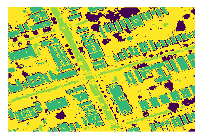
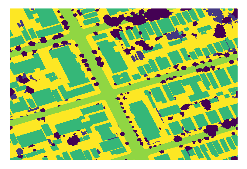
Figure 3: Rule-based land cover classification utilizing rasterized LiDAR statistics (top, cf. Secs. IV-A, IV-B) compared to the ground truth (bottom, cf. Sec. III-B) exemplified by a block in the neighborhood Corona, Queens, NYC. Qualitatively, the classification by LiDAR data statistics reproduces the scene containing buildings, vegetation, and roads. Quantitative measures, cf. Tab. III and Fig. 4, indicate noise for which its root is detailed in Sec. IV-C and Fig. 5.

IV-C Validation of Automated Label Generation

A quantitative analysis of accuracy reveals the combination of Fig. 4 and Tab. III. In particular, for each class detected, we compute the binary classification accuracy measures precision $P$ and recall $R$ according to

$$P=\frac{TP}{TP+FP}\quad\text{and}\quad R=\frac{TP}{TP+FN}\quad.$$ (1)

Given the Land Cover ground truth labels (cf. Sec. III-B) and a class to evaluate (here: roads, buildings, or vegetation), precision $P$ defines the amount of rule-based labeled pixels correctly identified (true positive: $TP$) in proportion to all pixels labeled as given class (type I error, false positive: $FP$). Similarly, recall $R$ encodes type II errors (false negative: $FN$) by forming the ratio of all true positive pixels relative to all ground truth pixels of a class. Accordingly, overall (class-specific) accuracy $acc$ is defined by all the truly classified pixels ($TP+TN$, with true negative: $TN$) in proportion to the total number of pixels:

$$acc=\frac{TP+TN}{TP+TN+FP+FN}\quad.$$ (2)

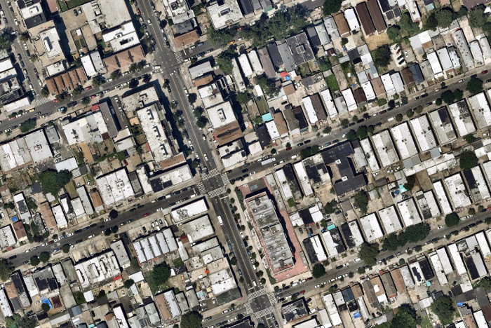
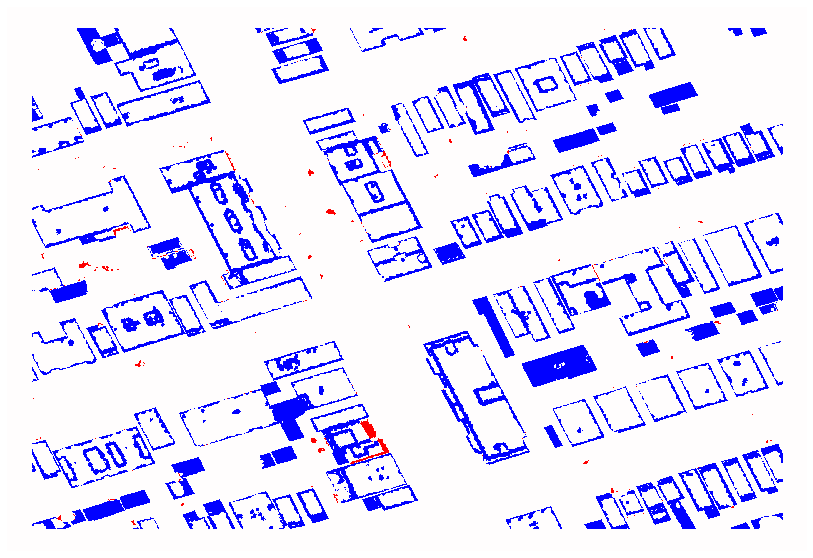
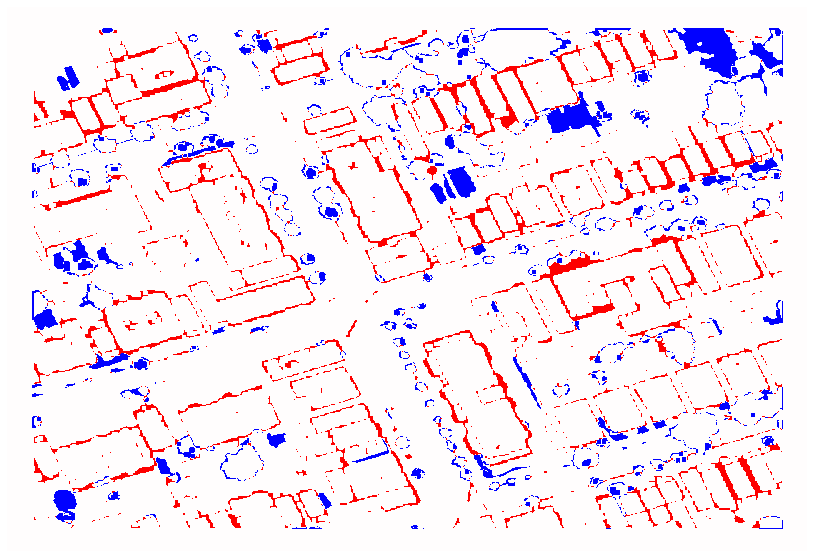
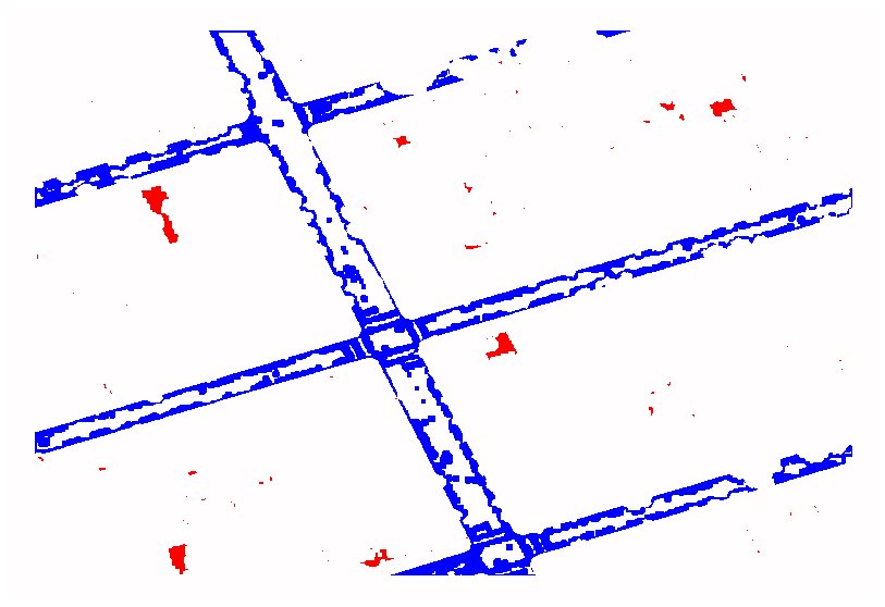
Figure 4: Visual accuracy evaluation of rule-based labeling from LiDAR measurements of the urban block exemplified in Fig. 3. The top left orthophoto provides a visual impression of the scene. The remaining sub-figures separately investigate the accuracy of buildings (top right), vegetation (bottom left), and roads (bottom right). White color coding marks correct labeling, blue brands missed labels (false negative, $FN$), and red distinguishes incorrect class labelling (false positive, $FP$). Tab. III quantifies the assessment.

As visually depicted in Fig. 4, identification of buildings and roads is dominated by false negatives (blue). Reversely, false positives (red) govern identification of vegetation. For labeling of buildings and vegetation such inverse relation of $FP$ and $FN$ roots in the physical reflectance properties of the LiDAR measurements at the edge of buildings: As the laser partially hits the outline of a building, multiple pulses get reflected back to the detector from the rooftop, the building’s face, and the ground—a scenario the rule-based labeling for vegetation in Tab. II is sensitive to. In fact, this source of label noise might get exploited for building footprint extraction utilizing traditional computer vision (post-)processing steps such as morphological filtering [46] or a straight line detector [47].

Except for the building edge labeling artefact, low false positive/negative rates on bulk objects such as buildings and vegetation allow for a relatively high $F_{1}$ score determined by the harmonic mean of precision and recall:

$$F_{1}=\frac{1}{\frac{1}{2}(1/P+1/R)}=\frac{2PR}{P+R}\quad.$$ (3)

Nevertheless, a fourth quantity, the Intersection over Union ($IoU$) is required to complement the accuracy evaluation:

$$IoU=\frac{|C\cap T|}{|C\cup T|}\quad,$$ (4)

with $C$ the set of rule-based labels of a given class, and $T$ the corresponding ground truth. $|\cdot|$ denotes the set size operator which returns geospatial area covered. This way, it is measured the degree of spatial misalignment of rule-based labels wrt. the ground truth. Since label noise dominates at the boundary of classification objects, $IoU$ scores low for buildings and vegetation. Results for road labeling suffer from covering vegetation and curb noise such as parked vehicles, power lines, traffic lights, light poles, etc.

However, as Fig. 3 visually demonstrates, the bulk of objects gets correctly labeled by the rule-based approach. A fact imprinted in the $acc$-measure for each class. Hence, we propose a challenge to the large-scale data mining remote sensing community: employ rule-based rasterized LiDAR statistics as automatically generated, noisy labels to benchmark weakly supervised semantic segmentation methodologies. In particular, the NAIP orthoimages [48] in combination with the NYC LiDAR data [30] provides model input.

TABLE III: Accuracy Assessment of rule-based Labeling

class	precision $P$	recall $R$	$F_{1}$-score	acc	Intersection
					over Union $IoU$
buildings	.98	.62	.76	.88	.61
vegetation	.52	.60	.55	.90	.38
roads	.91	.44	.59	.93	.42

IV-D LiDAR Statistics Clustering for Label Generation

To further investigate the label noise, we visualize data clustering in the multi–dimensional space of rasterized LiDAR statistics. Specifically, we utilized the $13$ raw statistics features $X=(A,B,\dots,M)$ of Tab. I to non-linearly project these into two dimensions for plotting through t-Distributed Stochastic Neighbor Embedding (t-SNE) [49]: $(x,y)=tSNE(X)$. Random sampling of geo-locations generates a ground-truth $l\in\{\text{building},\text{road},\text{vegetation}\}$ labeled set of data points $\{(X_{1},l_{1}),(X_{2},l_{2}),(X_{3},l_{3}),\dots\}$. The corresponding t-SNE projection $\{(x_{1},y_{1}),(x_{2},y_{2}),(x_{3},y_{3}),\dots\}$ is presented in Fig. 5 with color coding $\{l_{1},l_{2},l_{3},\dots\}$.

While cluster sizes and distances between strongly depend on t-SNE initial conditions and parameter settings, qualitative cluster structure in high-dimensional space may get read off from the two-dimensional embedding. In particular, we ran t-SNE experiments with various settings and differing data samplings. Repeatedly, it yielded qualitatively similar results as exemplified by Fig. 5: The three classes associated with vegetation, buildings, and roads are well separated. Thus, distinct sets of classes can be defined through a combination of LiDAR statistics layers in order to identify those. However, standard clustering methods like $k$-means—even when adapted to variable number of clusters [50]—is likely to fail due to the highly nonlinear separation of classes: As apparent from Fig. 5, a single class like vegetation is associated with a number of clusters well separated.

Highly non-linear functions can get modelled by artificial neural networks. Research in self-supervised learning recently demonstrated the generation of expressive feature vectors without the need for any labels [51]. Performance of self-supervised learning is typically measured by the accuracy of downstream tasks that employ the learnt feature representation $z$. Specifically, object classification is evaluated by training a single-layer of fully connected neurons attached to $z$ on a small set of ground truth labels. Hence, a future research direction in AutoGeoLabel may exploit self-supervised learning to improve upon the noisy, rule-based label generation process with the aid of a small set of ground truth labels.

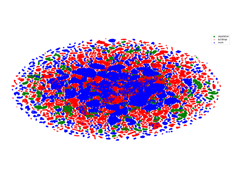
Figure 5: t-SNE embedding of the $13$–dimensional LiDAR raster statistics, cf. Tab. I. Randomly picked land classification samples of vegetation (green, $\boldsymbol{\cdot}$), buildings (red, $\cdot$), and roads (blue, $+$) is plotted. It becomes apparent that near to perfect class separation requires a strongly non-linear function such as e.g. modelled by artificial neural networks.

V Application

We demonstrate an industrial application of labels generated by AutoGeoLabel to identify trees and quantify carbon sequestration [52, 53]. LiDAR statistics can identify tree’s location, extract canopy diameter and calculate the total carbon sequestered in trees. AutoGeoLabel-generated vegetation labels are converted to polygons. Subsequently, the mask is used to crop the maximum elevation LiDAR statistics data, $e_{+}$. The obtained image with vegetation height is segmented using a watershed method to delineate the tree crown diameter [54]. Then, the tree crown polygons can be used as another simple filter layer where the eccentricity [55] of polygons helps to eliminate features that appears elongated to preserve rounded/circular features, only. In addition, filtering is employed to remove features that are too small or too large to be associated with a tree.

Manually labeled tree species data is used to create a classifier associating tree species labels [56]. Four dominant tree species are used to reclassify all trees within NYC [53]. Tree height is extracted from the LiDAR height where the height is adjusted taking into account the ground elevation—resulting in absolute tree height.

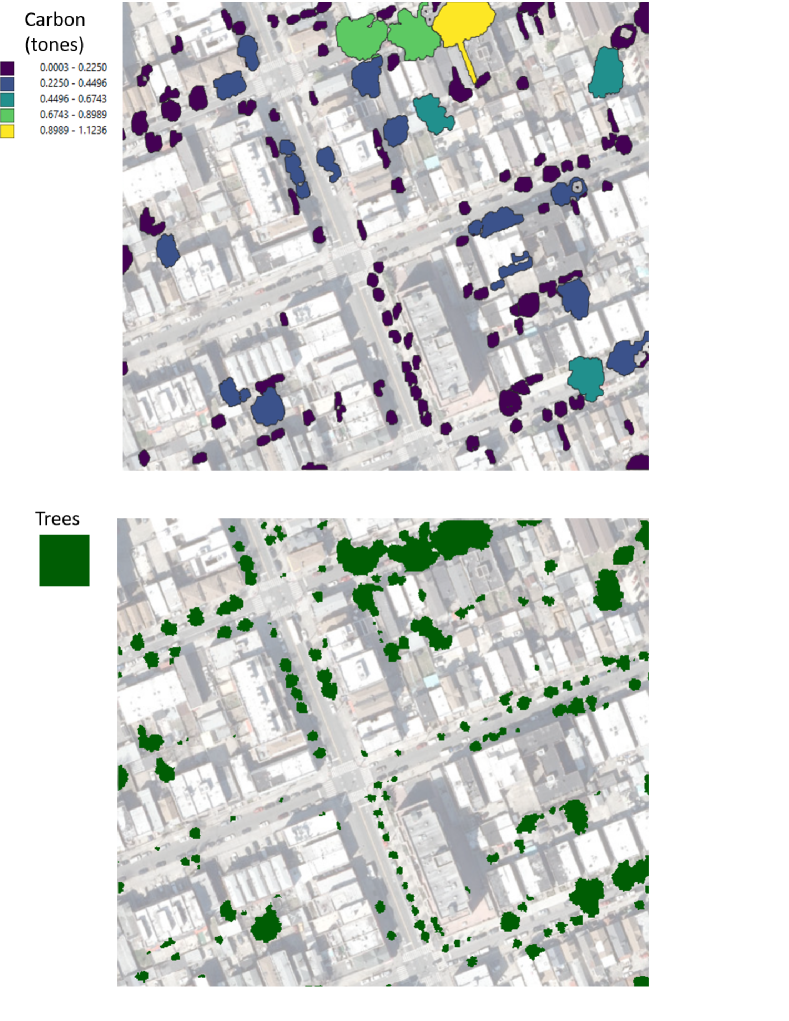
Figure 6: Application: Total carbon stored in trees (top) calculated based on tree species and tree dimensions derived from LiDAR measurements for geospatial sample area of Fig. 3. The corresponding ground truth image (bottom) depicts the distribution of the urban forest, cf. Fig. 3 (bottom).

Quantification of carbon stored in trees follows a procedure outlined before [53]. The method presented here is different from previous works as it exclusively relies on LiDAR data to identify vegetation using automatically created labels, delineate tree canopy, and calculate tree heights. The only additional data required is tree species information [56, 53]. Tree identification and carbon sequestration offer a way for city management to better plan tree replanting, and to efficiently quantify total carbon stored in urban forest.

VI Conclusion & Perspectives

In this paper we presented AutoGeoLabel; a framework to address automatic data labeling for geospatial applications. Many industrial and scientific solutions can benefit from automating label generation to overcome the challenge of manual image annotation—a labor- and time-consuming effort. Based on an airborne LiDAR survey for New York City, we demonstrated and explored a novel approach to use simple statistical features of remote sensing data in order to create data classes. Weakly supervised, and self-supervised learning has been argued as promising approaches. Utilizing automatically generated labels for vegetation, we demonstrated an application to quantify carbon sequestration in urban forests with no need for explicit tree segmentation from e.g. orthophotos.

In perspective of industry applications, there is great potential of AutoGeoLabel to contribute. E.g. for emergency response during a natural disaster event, many of the existing labeled data acquired under normal conditions may not hold representative of what it is observed on the ground. In such extreme situations, new labeled data may need to be generated on the fly. One such example is recognizing flooded areas utilizing aerial, or drone images where training data may not exist. Detecting the impact of extreme weather can drive rescue missions, where assessment of change from normal conditions like water extent and potential damage (estimates of depth of water) require creation of data features that can be used to delineate the boundary of overflown water. Then, information related to the number of flooded houses and roads may help to coordinate the best routing for rescue missions.

References

- [1] I. Z. Yalniz, H. Jégou, K. Chen, M. Paluri, and D. Mahajan, “Billion-scale semi-supervised learning for image classification,” arXiv preprint arXiv:1905.00546, 2019.
- [2] A. Krizhevsky, I. Sutskever, and G. E. Hinton, “Imagenet classification with deep convolutional neural networks,” Advances in neural information processing systems, vol. 25, pp. 1097–1105, 2012.
- [3] T.-Y. Lin, M. Maire, S. Belongie, J. Hays, P. Perona, D. Ramanan, P. Dollár, and C. L. Zitnick, “Microsoft coco: Common objects in context,” in European conference on computer vision. Springer, 2014, pp. 740–755.
- [4] L. Deng, “The mnist database of handwritten digit images for machine learning research [best of the web],” IEEE Signal Processing Magazine, vol. 29, no. 6, pp. 141–142, 2012.
- [5] O. A. Penatti, K. Nogueira, and J. A. Dos Santos, “Do deep features generalize from everyday objects to remote sensing and aerial scenes domains?” in Proceedings of the IEEE conference on computer vision and pattern recognition workshops, 2015, pp. 44–51.
- [6] G. Cheng, X. Xie, J. Han, L. Guo, and G.-S. Xia, “Remote sensing image scene classification meets deep learning: Challenges, methods, benchmarks, and opportunities,” IEEE Journal of Selected Topics in Applied Earth Observations and Remote Sensing, vol. 13, pp. 3735–3756, 2020.
- [7] E. Maggiori, Y. Tarabalka, G. Charpiat, and P. Alliez, “Convolutional neural networks for large-scale remote-sensing image classification,” IEEE Transactions on geoscience and remote sensing, vol. 55, no. 2, pp. 645–657, 2016.
- [8] W. Zhou and L. J. Klein, “Monitoring the impact of wildfires on tree species with deep learning,” in Neural Information Processing Systems (NeurIPS 2020) Workshop, 2020. [Online]. Available: https://arxiv.org/abs/2011.02514
- [9] M. Reichstein, G. Camps-Valls, B. Stevens, M. Jung, J. Denzler, and N. Carvalhais, “Deep learning and process understanding for data-driven earth system science,” Nature, vol. 566, pp. 195–204, 2019.
- [10] D. Mahajan, R. Girshick, V. Ramanathan, K. He, M. Paluri, Y. Li, A. Bharambe, and L. Van Der Maaten, “Exploring the limits of weakly supervised pretraining,” in Proceedings of the European conference on computer vision (ECCV), 2018, pp. 181–196.
- [11] A. T. Hudak, J. S. Evans, and A. M. Stuart Smith, “Lidar utility for natural resource managers,” Remote Sensing, vol. 1, no. 4, pp. 934–951, 2009.
- [12] A. Paszke, S. Gross, S. Chintala, G. Chanan, E. Yang, Z. DeVito, Z. Lin, A. Desmaison, L. Antiga, and A. Lerer, “Automatic differentiation in pytorch,” 2017.
- [13] M. Abadi, A. Agarwal, P. Barham, E. Brevdo, Z. Chen, C. Citro, G. S. Corrado, A. Davis, J. Dean, M. Devin, S. Ghemawat, I. Goodfellow, A. Harp, G. Irving, M. Isard, Y. Jia, R. Jozefowicz, L. Kaiser, M. Kudlur, J. Levenberg, D. Mané, R. Monga, S. Moore, D. Murray, C. Olah, M. Schuster, J. Shlens, B. Steiner, I. Sutskever, K. Talwar, P. Tucker, V. Vanhoucke, V. Vasudevan, F. Viégas, O. Vinyals, P. Warden, M. Wattenberg, M. Wicke, Y. Yu, and X. Zheng, “TensorFlow: Large-scale machine learning on heterogeneous systems,” 2015, software available from tensorflow.org. [Online]. Available: https://www.tensorflow.org/
- [14] G. Büttner, J. Feranec, G. Jaffrain, C. Steenmans, A. Gheorghe, and V. Lima, “Corine land cover update 2000,” Technical guidelines, 2002.
- [15] J. Wickham, C. Homer, J. Vogelmann, A. McKerrow, R. Mueller, N. Herold, and J. Coulston, “The multi-resolution land characteristics (mrlc) consortium—20 years of development and integration of usa national land cover data,” Remote Sensing, vol. 6, no. 8, pp. 7424–7441, 2014.
- [16] J. Shermeyer, D. Hogan, J. Brown, A. Etten, N. Weir, F. Pacifici, R. Hänsch, A. Bastidas, S. Soenen, T. Bacastow, and R. Lewis, “Spacenet 6: Multi-sensor all weather mapping dataset,” in 2020 IEEE/CVF Conference on Computer Vision and Pattern Recognition Workshops (CVPRW), 2020, pp. 768–777.
- [17] G. Sumbul, M. Charfuelan, B. Demir, and V. Markl, “Bigearthnet: A large-scale benchmark archive for remote sensing image understanding,” CoRR, vol. abs/1902.06148, 2019.
- [18] S. Basu, S. Ganguly, S. Mukhopadhyay, R. DiBiano, M. Karki, and R. Nemani, “Deepsat: a learning framework for satellite imagery,” in Proceedings of the 23rd SIGSPATIAL international conference on advances in geographic information systems, 2015, pp. 1–10.
- [19] “Open street map (osm).” [Online]. Available: https://wiki.openstreetmap.org/wiki/Map_features
- [20] C. M. Albrecht, R. Zhang, X. Cui, M. Freitag, H. F. Hamann, L. J. Klein, and et al., “Change detection from remote sensing to guide openstreetmap labeling,” ISPRS International Journal of Geo-Information, vol. 9, p. 427, 2020.
- [21] R. Zhang, C. Albrecht, W. Zhang, X. Cui, U. Finkler, D. Kung, and S. Lu, “Map generation from large scale incomplete and inaccurate data labels,” in Proceedings of the 26th ACM SIGKDD International Conference on Knowledge Discovery & Data Mining, 2020, pp. 2514–2522.
- [22] P. O. Gislason, J. A. Benediktsson, and J. R. Sveinsson, “Random forests for land cover classification,” Pattern recognition letters, vol. 27, no. 4, pp. 294–300, 2006.
- [23] C. Huang, L. Davis, and J. Townshend, “An assessment of support vector machines for land cover classification,” International Journal of remote sensing, vol. 23, no. 4, pp. 725–749, 2002.
- [24] S. Shekhar, P. R. Schrater, R. R. Vatsavai, W. Wu, and S. Chawla, “Spatial contextual classification and prediction models for mining geospatial data,” IEEE Transactions on Multimedia, vol. 4, no. 2, pp. 174–188, 2002.
- [25] X. X. Zhu, D. Tuia, L. Mou, G.-S. Xia, L. Zhang, F. Xu, and F. Fraundorfer, “Deep learning in remote sensing: A comprehensive review and list of resources,” IEEE Geoscience and Remote Sensing Magazine, vol. 5, no. 4, pp. 8–36, 2017.
- [26] P. Bolstad, GIS fundamentals: A first text on geographic information systems. Eider (PressMinnesota), 2016.
- [27] S. Madakam, V. Lake, V. Lake, V. Lake et al., “Internet of things (iot): A literature review,” Journal of Computer and Communications, vol. 3, no. 05, p. 164, 2015.
- [28] J. Chen and X. Ran, “Deep learning with edge computing: A review.” Proc. IEEE, vol. 107, no. 8, pp. 1655–1674, 2019.
- [29] “Open topography).” [Online]. Available: https://www.opentopography.org/
- [30] “New york city lidar, 2017.” [Online]. Available: https://maps.nyc.gov/lidar/2017/
- [31] The Imaging & Geospatial Information Society, “Asprs las specification,” https://github.com/ASPRSorg/LAS, 2019.
- [32] “Land cover nyc, 2017.” [Online]. Available: https://data.cityofnewyork.us/Environment/Land-Cover-Raster-Data-2017-6in-Resolution/he6d-2qns
- [33] H. Tenkanen, E. Di Minin, V. Heikinheimo, A. Hausmann, M. Herbst, L. Kajala, and T. Toivonen, “Instagram, flickr, or twitter: Assessing the usability of social media data for visitor monitoring in protected areas,” Scientific reports, vol. 7, no. 1, pp. 1–11, 2017.
- [34] N. Gorelick, M. Hancher, M. Dixon, S. Ilyushchenko, D. Thau, and R. Moore, “Google earth engine: Planetary-scale geospatial analysis for everyone,” Remote sensing of Environment, vol. 202, pp. 18–27, 2017.
- [35] M. Sudmanns, D. Tiede, S. Lang, H. Bergstedt, G. Trost, H. Augustin, A. Baraldi, and T. Blaschke, “Big earth data: disruptive changes in earth observation data management and analysis?” International Journal of Digital Earth, vol. 13, no. 7, pp. 832–850, 2020.
- [36] A. L. Luers, “Planetary intelligence for sustainability in the digital age: Five priorities,” One Earth, vol. 4, no. 6, pp. 772–775, 2021.
- [37] M. A. Whitby, R. Fecher, and C. Bennight, “Geowave: Utilizing distributed key-value stores for multidimensional data,” in International Symposium on Spatial and Temporal Databases. Springer, 2017, pp. 105–122.
- [38] L. J. Klein, F. J. Marianno, C. M. Albrecht, M. Freitag, S. Lu, N. Hinds, X. Shao, S. B. Rodriguez, and H. F. Hamann, “Pairs: A scalable geo-spatial data analytics platform,” in 2015 IEEE International Conference on Big Data (Big Data). IEEE, 2015, pp. 1290–1298.
- [39] W. Zhou, L. J. Klein, and S. Lu, “Pairs autogeo: an automated machine learning framework for massive geospatial data,” in 2020 IEEE International Conference on Big Data (Big Data). IEEE, 2020, pp. 1755–1763.
- [40] A. Maas, F. Rottensteiner, and C. Heipke, “Using label noise robust logistic regression for automated updating of topographic geospatial databases,” in XXIII ISPRS Congress, Commission VII 3 (2016), Nr. 7, vol. 3, no. 7. Göttingen: Copernicus GmbH, 2016, pp. 133–140.
- [41] F. Warmerdam, “The geospatial data abstraction library,” pp. 87–104, 2008.
- [42] H. Butler, B. Chambers, P. Hartzell, and C. Glennie, “Pdal: An open source library for the processing and analysis of point clouds,” Computers & Geosciences, vol. 148, p. 104680, 2021.
- [43] C. R. Harris, K. J. Millman, S. J. van der Walt, R. Gommers, P. Virtanen, D. Cournapeau, E. Wieser, J. Taylor, S. Berg, N. J. Smith, R. Kern, M. Picus, S. Hoyer, M. H. van Kerkwijk, M. Brett, A. Haldane, J. Fernández del Río, M. Wiebe, P. Peterson, P. Gérard-Marchant, K. Sheppard, T. Reddy, W. Weckesser, H. Abbasi, C. Gohlke, and T. E. Oliphant, “Array programming with NumPy,” Nature, vol. 585, p. 357–362, 2020.
- [44] IBM, “Ibm pairs geoscope open source modules,” https://github.com/ibm/ibmpairs, 2019.
- [45] C. M. Albrecht, C. Fisher, M. Freitag, H. F. Hamann, S. Pankanti, F. Pezzutti, and F. Rossi, “Learning and recognizing archeological features from lidar data,” in 2019 IEEE International Conference on Big Data (Big Data). IEEE, 2019, pp. 5630–5636.
- [46] O. Sigmund, “Morphology-based black and white filters for topology optimization,” Structural and Multidisciplinary Optimization, vol. 33, no. 4-5, pp. 401–424, 2007.
- [47] N. Kiryati, Y. Eldar, and A. M. Bruckstein, “A probabilistic hough transform,” Pattern recognition, vol. 24, no. 4, pp. 303–316, 1991.
- [48] “National agriculture imagery program, data download.” [Online]. Available: https://www.fsa.usda.gov/programs-and-services/aerial-photography/imagery-programs/naip-imagery/
- [49] L. van der Maaten and G. Hinton, “Visualizing data using t-sne,” Journal of Machine Learning Research, vol. 9, no. 86, pp. 2579–2605, 2008. [Online]. Available: http://jmlr.org/papers/v9/vandermaaten08a.html
- [50] G. Hamerly and C. Elkan, “Learning the k in k-means,” Advances in neural information processing systems, vol. 16, pp. 281–288, 2004.
- [51] L. Jing and Y. Tian, “Self-supervised visual feature learning with deep neural networks: A survey,” IEEE transactions on pattern analysis and machine intelligence, 2020.
- [52] L. J. Klein, C. M. Albrecht, W. Zhou, C. Siebenschuh, S. Pankanti, H. F. Hamann, and S. Lu, “N-dimensional geospatial data and analytics for critical infrastructure risk assessment,” in 2019 IEEE International Conference on Big Data (Big Data). IEEE, 2019, pp. 5637–5643.
- [53] L. Klein, W. Zhou, and C. Albrecht, “Quantification of carbon sequestration in urban forests,” arXiv preprint arXiv:2106.00182, 2021.
- [54] L. Wang, P. Gong, and G. S. Biging, “Individual tree-crown delineation and treetop detection in high-spatial-resolution aerial imagery,” Photogrammetric Engineering & Remote Sensin, vol. 70, no. 3, pp. 351–357, 2004.
- [55] “Eccentricity (mathematics).” [Online]. Available: https://en.wikipedia.org/wiki/Eccentricity_(mathematics)
- [56] NYC-Street-Tree-Map, “New york city street tree map,” New York City, NY, Tech. Rep., 2015. [Online]. Available: https://tree-map.nycgovparks.org/