Monte Carlo stochastic Galerkin methods for non-Maxwellian kinetic models of multiagent systems with uncertainties

Abstract

In this paper, we focus on the construction of a hybrid scheme for the approximation of non-Maxwellian kinetic models with uncertainties. In the context of multiagent systems, the introduction of a kernel at the kinetic level is useful to avoid unphysical interactions. The methods here proposed, combine a direct simulation Monte Carlo (DSMC) in the phase space together with stochastic Galerkin (sG) methods in the random space. The developed schemes preserve the main physical properties of the solution together with accuracy in the random space. The consistency of the methods is tested with respect to surrogate Fokker-Planck models that can be obtained in the quasi-invariant regime of parameters. Several applications of the schemes to non-Maxwellian models of multiagent systems are reported.

Keywords: uncertainty quantification; stochastic Galerkin methods; Direct Simulation Monte Carlo methods; nonlinear Fokker-Planck equations; kinetic equations; kinetic modelling

1 Introduction

Kinetic equations are often studied to describe aggregate trends of large systems of interacting particles and have shown a remarkable effectivity in different research fields, ranging from classical rarefied gas dynamics to socio-economic and traffic flow dynamics. Without reviewing the huge literature on these topics, we mention [6, 9, 7, 12, 14, 37, 42, 43] and the reference therein for an introduction to the subject. The contributions have to be further distinguished depending on the type of kernel characterizing the interaction frequency between particles or agents. It is worth mentioning that the introduction of a state-dependent kernel represents an essential tool in kinetic theory to enforce physical properties of rarefied gases [13], whereas it is currently underexplored in less classical applications to multi-agent systems. In this direction, we mention the following recent contributions [21, 20, 18, 23].

The deterministic description of multi-agent phenomena has often to face the lack of essential information on microscopic dynamics, initial states, or boundary conditions. Hence, it is of paramount importance to quantify and control possible deviations from expected trends and patterns due to unavoidable uncertainties in the model parameters and initial distributions. An established idea relies on considering these quantities as random variables influencing the evolution of the kinetic distribution, increasing, therefore, the dimensionality of the problem. In recent years, we experienced a growing interest in the construction of numerical methods for kinetic equations with uncertainties, see the collection [31]. Among the most popular techniques for uncertainty quantification, stochastic Galerkin (sG) methods are based on the construction of deterministic solvers and are capable to guarantee spectral convergence in the random field under suitable regularity assumptions [34, 28, 53]. Anyway, their computational cost is generally high due to the curse of dimensionality of kinetic equations and they are highly intrusive with respect to the original formulation of the model. Furthermore, the main physical properties of the solution, like its positivity, entropy dissipation, and hyperbolicity, are lost. Besides sG methods, we find nonintrusive approaches to UQ that do not require significant modifications to the numerical scheme of the deterministic problem and are based on collocation strategies. Therefore, these latter methods are easy to parallelize and do not require any knowledge of the class of probability distributions of random parameters. In this direction, multi-fidelity approaches have been recently developed using control variate techniques, see [4, 15, 16, 29, 24, 38].

In this work, we follow a different path that is inspired by the novel approach proposed in the seminal work for mean-field equations [8] and further extended to the homogeneous Boltzmann equation in [40]. The proposed approach is capable to combine the efficiency of Direct Simulation Monte Carlo (DSMC) methods for nonlinear kinetic equations in the phase space [2, 1, 35, 36] with the accuracy of sG methods in the parameter space. The DSMC-sG method preserves the main physical properties of the kinetic solution along with spectral accuracy in the random space provided minimal regularity assumptions. Anyway, in a non-Maxwellian framework, the numerical formulation of the DSMC-sG method requires the introduction of step functions at the particles’ level. As shown in [40] for the variable hard-spheres (VHS) model, this fact can break spectral convergence of sG. For this reason, it has been shown that a mollification of the step function coupled with a thermalization of particles is capable to restore the physical validity of the model together with spectral accuracy in the random space.

In models for collective phenomena, the equilibrium distribution of Boltzmann-type models is unknown and typically only mass is conserved. For this reason, we introduce a surrogate Fokker-Planck model that can be formally derived from the original model in the quasi-invariant limit [45]. In the case of non-Maxwellian interactions, we will obtain a nonlocal nonlinear Fokker-Planck class of equations whose equilibrium distribution can be approximated numerically through suitable deterministic methods [39]. In particular, we will investigate the effects of a mollification of step functions introduced at the Monte Carlo level, coupled with a correction of nonconserved quantities computed by the approximation of the corresponding surrogate Fokker-Planck model. Numerical tests for kinetic models of wealth distribution and traffic flow have been performed.

The rest of the paper is organized as follows. In Section 2 we introduce non-Maxwellian models for multi-agent systems with random inputs and we formally derive their corresponding Fokker-Planck models. Regularity of the solutions in the random space of the surrogate models has been investigated in Section 2.2. In Section 3 we briefly review the basic features of some existing kinetic models for pure gambling, wealth distribution and traffic flow dynamics with non-Maxwellian kernels. In Section 4 then we construct the DSMC-sG methods and we provide results on the consistency of the method. Finally, in Section 5 several numerical results are presented which show the efficiency and accuracy of the introduced method.

2 Non-Maxwellian models with uncertain parameters

To introduce the modelling setting we consider a binary interaction model with uncertain mixing [17, 46, 38]. If two sampled particles that are characterized by the pre-interaction states $v,w\in\mathbb{V}\subseteq\mathbb{R}$ interact, then their post-interaction states $v^{\prime},w^{\prime}\in\mathbb{V}$ are obtained following the scheme

$$\begin{split}v^{\prime}=v-\epsilon I_{1}(v,w,\mathbf{z})+D_{1}(v)\eta_{\epsilon},\\ w^{\prime}=w-\epsilon I_{2}(v,w,\mathbf{z})+D_{2}(w)\eta_{\epsilon},\end{split}$$ (1)

with $\epsilon>0$ a given constant, $I_{1}$, $I_{2}$ suitable interaction functions depending on the pre-interaction states and on the random quantity $\mathbf{z}\in\mathbb{R}^{d_{\mathbf{z}}}$, $d_{\mathbf{z}}\geq 1$. Furthermore, $\eta_{\epsilon}$ is a random variable with zero mean and variance $\sigma_{\epsilon}^{2}$, and the functions $D_{1}$ and $D_{2}$ define the local relevance of the diffusion. Under suitable assumptions on the strength of the diffusion it is possible to show that the post-interaction states $v^{\prime}$, $w^{\prime}$ remain in $\mathbb{V}$.

We adopt a classical kinetic theory approach based on the one-dimensional space-homogeneous Boltzmann equation, that describes the time evolution of the one-body distribution function $f=f(t,v,\mathbf{z})$. The function $f(t,v,\mathbf{z})$ identifies the state of the system, such that $f(t,v,\mathbf{z})dv$ is the fraction of agents characterized by a state comprised between $v$ and $v+dv$ at time $t>0$ and parametrised by uncertainties defined in the random vector $\mathbf{z}$ with joint distribution $p(\mathbf{z})$. The evolution of $f$ is given by the non-Maxwellian Boltzmann-type model

$$\begin{split}&\dfrac{d}{dt}\int_{\mathbb{V}}\varphi(v)f(t,v,\mathbf{z})dv\\ &\qquad=\dfrac{1}{2}\left\langle\iint_{\mathbb{V}\times\mathbb{V}}B(v,w,\mathbf{z})(\varphi(v^{\prime})+\varphi(w^{\prime})-\varphi(v)-\varphi(w))f(t,v,\mathbf{z})f(t,w,\mathbf{z})dvdw\right\rangle,\end{split}$$ (2)

where $\varphi:\mathbb{V}\rightarrow\mathbb{R}$ is a test function, while the symmetric function $B(v,w,\mathbf{z})$ denotes the collision kernel that characterizes the collision frequency of agents with states $v$ and $w$. The notation $\langle\cdot\rangle$ expresses the expectation with respect to the random variable $\eta_{\epsilon}$. The model introduced in (2) can be complemented with uncertain initial condition $f(0,v,\mathbf{z})=f_{0}(v,\mathbf{z})$.

It is worth noting that in the VHS framework of classical kinetic theory for rarefied gas dynamics the collisional kernel is assumed to be function of the relative velocity $|v-w|$, see [9]. The model (2) greatly simplifies in the Maxwellian case corresponding to $B(v,w,\mathbf{z})\equiv 1$. In the description of collective models in the Maxwellian simplification of considering a constant interaction kernel has been largely considered [22, 37, 47, 49]. Within the Maxwellian simplification it is possible to argue on the existence and uniqueness of large time behavior of the resulting model. In some cases, explicit solutions can be obtained, as in the famous one-dimensional Kac model [32]. In models for collective phenomena, a precise analytical description of the kinetic emerging equilibrium distribution is very difficult to obtain. A possible way to overcome this difficulty relies on the possibility to study surrogate models, that are approximations of the kinetic model (2) in some limit and whose large time behavior is easily available.

2.1 Fokker-Planck approximation

The computation of the emerging equilibrium density of the Boltzmann model introduced in (2) is very challenging. An established way to overcome this difficulty relies on the introduction of the quasi-invariant limit [11, 45, 46] under which it is possible to derive a surrogate Fokker-Planck model for the interaction dynamics. The introduced scaling has connections with the grazing collision limit in classical kinetic theory. The main idea is to introduce a new time scale $\tau=\epsilon t$ and to define

$$f_{\epsilon}(\tau,v,\mathbf{z})=f(\tau/\epsilon,v,\mathbf{z})$$

that is solution to

$$\begin{split}&\dfrac{d}{d\tau}\int_{\mathbb{V}}\varphi(v)f_{\epsilon}(\tau,v,\mathbf{z})dv\\ &\qquad=\dfrac{1}{2\epsilon}\left\langle\iint_{\mathbb{V}^{2}}B(v,w,\mathbf{z})(\varphi(v^{\prime})+\varphi(w^{\prime})-\varphi(v)-\varphi(w))f_{\epsilon}(\tau,v,\mathbf{z})f_{\epsilon}(\tau,w,\mathbf{z})dv\,dw\right\rangle.\end{split}$$ (3)

Hence, scaling the variance of the random variable $\eta_{\epsilon}$ as $\sigma_{\epsilon}^{2}=\epsilon\sigma^{2}$ we have that for $\epsilon\ll 1$ the interaction dynamics in (1) are quasi-invariant, since $v^{\prime}-v\ll 1$ and $w^{\prime}-w\ll 1$. Assuming then $\varphi$ smooth enough and at least $\varphi\in\mathbb{C}_{0}^{3}(\mathbb{V})$, we can perform the following Taylor expansions

$$\begin{split}\varphi(v^{\prime})-\varphi(v)&=(v^{\prime}-v)\dfrac{d}{dv}\varphi(v)+\dfrac{1}{2}(v^{\prime}-v)^{2}\dfrac{d^{2}}{dv^{2}}\varphi(v)+\dfrac{1}{6}(v^{\prime}-v)^{3}\dfrac{d^{3}}{dv^{3}}\varphi(\bar{v})\\ \varphi(w^{\prime})-\varphi(w)&=(w^{\prime}-w)\dfrac{d}{dw}\varphi(w)+\dfrac{1}{2}(w^{\prime}-w)^{2}\dfrac{d^{2}}{dw^{2}}\varphi(w)+\dfrac{1}{6}(w^{\prime}-w)^{3}\dfrac{d^{3}}{dw^{3}}\varphi(\bar{w}),\end{split}$$

with $\bar{v}\in(\textrm{min}\{v,v^{\prime}\},\textrm{max}\{v,v^{\prime}\})$, $\bar{w}\in(\textrm{min}\{w,w^{\prime}\},\textrm{max}\{w,w^{\prime}\})$. Plugging the above expansion in (3) we obtain

$$\begin{split}&\dfrac{d}{d\tau}\int_{\mathbb{V}}\varphi(v)f_{\epsilon}(\tau,v,\mathbf{z})dv\\ &=\dfrac{1}{2\epsilon}\left\{\left\langle\iint_{\mathbb{V}^{2}}B(v,w,\mathbf{z})\left[(v^{\prime}-v)\dfrac{d}{dv}\varphi(v)+(w^{\prime}-w)\dfrac{d}{dw}\varphi(w)\right]f_{\epsilon}(\tau,v,\mathbf{z})f_{\epsilon}(\tau,w,\mathbf{z})dv\,dw\right\rangle\right.\\ &+\dfrac{1}{2\epsilon}\left.\left\langle\iint_{\mathbb{V}^{2}}B(v,w,\mathbf{z})\left[(v^{\prime}-v)^{2}\dfrac{d^{2}}{dv^{2}}\varphi(v)+(w^{\prime}-w)^{2}\dfrac{d^{2}}{dw^{2}}\varphi(w)\right]f_{\epsilon}(\tau,v,\mathbf{z})f_{\epsilon}(\tau,w,\mathbf{z})dv\,dw\right\rangle\right\}\\ &+R_{\varphi}^{\epsilon}(f_{\epsilon},f_{\epsilon}),\end{split}$$

where $R_{\varphi}^{\epsilon}(f_{\epsilon},f_{\epsilon})$ is a reminder term of the following form

$$R_{\varphi}^{\epsilon}(f_{\epsilon},f_{\epsilon})=\dfrac{1}{6\epsilon}\left\langle\iint_{\mathbb{V}^{2}}B(v,w,\mathbf{z})\left[(v^{\prime}-v)^{3}\dfrac{d^{3}}{dv^{3}}\varphi(v)+(w^{\prime}-w)^{3}\dfrac{d^{3}}{dw^{3}}\varphi(w)\right]f_{\epsilon}(\tau,v,\mathbf{z})f_{\epsilon}(\tau,w,\mathbf{z})dv\,dw\right\rangle.$$

Thanks to the smoothness assumptions on $\varphi$ and the boundedness of the third order moment of $\eta_{\epsilon}$, in the limit $\epsilon\rightarrow 0$ we have that

$$|R_{\varphi}^{\epsilon}(f_{\epsilon},f_{\epsilon})|\rightarrow 0^{+}$$

and we may assume that $f_{\epsilon}$ converges to a distribution $f(\tau,v,\mathbf{z})$ at least formally, we point the interested reader to [7, 45] for related approaches in the Maxwellian and Boltzmann-Povzner frameworks. With a slight abuse of notation, we indicate with $f(\tau,v,\mathbf{z})$ the limit distribution as $\epsilon\rightarrow 0^{+}$, hence $f(\tau,v,\mathbf{z})$ is weak solution to the nonlinear nonlocal Fokker-Planck equation

$$\begin{split}&\partial_{\tau}f(\tau,v,\mathbf{z})=\partial_{v}\left[\int_{\mathbb{V}}B(v,w,\mathbf{z})(I_{1}(v,w,\mathbf{z})+I_{2}(v,w,\mathbf{z}))f(\tau,w,\mathbf{z})dwf(\tau,v,\mathbf{z})\right]\\ &\qquad{+}\dfrac{\sigma^{2}}{2}\partial_{v}^{2}\left[\int_{\mathbb{V}}B(v,w,\mathbf{z})f(\tau,w,\mathbf{z})dw(D^{2}_{1}(v)+D^{2}_{2}(v))f(\tau,v,\mathbf{z})\right],\end{split}$$ (4)

complemented with the following boundary conditions for all $\mathbf{z}\in\mathbb{R}^{d}$

$$\begin{split}&\int_{\mathbb{V}}B(v,w,\mathbf{z})(I_{1}(v,w,\mathbf{z})+I_{2}(v,w,\mathbf{z}))f(\tau,w,\mathbf{z})dwf(\tau,v,\mathbf{z})\\ &\qquad\qquad+\dfrac{\sigma^{2}}{2}\partial_{v}\left((D^{2}_{1}(v)+D^{2}_{2}(v))\int_{\mathbb{V}}B(v,w,\mathbf{z})f(\tau,w,\mathbf{z})dwf(\tau,v,\mathbf{z})\right)\Big{|}_{v\in\partial V}=0\\ &\int_{\mathbb{V}}B(v,w,\mathbf{z})f(\tau,w,\mathbf{z})dw(D^{2}_{1}(v)+D^{2}_{2}(v))f(\tau,v,\mathbf{z})\Big{|}_{v\in\partial V}=0\end{split}$$ (5)

2.2 Regularity of solutions in the random space

We recall that $p(\mathbf{z}):I_{\mathbf{z}}\rightarrow\mathbb{R}_{+}$ is the probability density of the random vector $\mathbf{z}$. We define the weighted norm in $L^{2}_{p}(\mathbb{V}\times I_{\mathbf{z}})$ as follows

$$\|f(t)\|_{L^{2}_{p}(\mathbb{V}\times I_{\mathbf{z}})}=\left(\int_{\mathbb{V}}\int_{I_{\mathbf{z}}}|f(t,v,\mathbf{z})|^{2}p(\mathbf{z})d\mathbf{z}dv\right)^{1/2}.$$

In the following we will provide sufficient conditions to guarantee regularity of the solution of the general Fokker-Planck model (4).

Let us rewrite first the Fokker-Planck models (4) as follows

$$\partial_{t}f(t,v,\mathbf{z})=\partial_{v}\left[\tilde{\mathcal{B}}[f](t,v,\mathbf{z})f(t,v,\mathbf{z})+\mathcal{D}[f](t,v,\mathbf{z})\partial_{v}(f(t,v,\mathbf{z}))\right],$$ (6)

with

$$\begin{split}\tilde{\mathcal{B}}[f](t,v,\mathbf{z})=&\int_{\mathbb{V}}B(v,w,\mathbf{z})(I_{1}(v,w,\mathbf{z})+I_{2}(v,w,\mathbf{z}))f(t,w,\mathbf{z})dw\\ &+\dfrac{\sigma^{2}}{2}(D_{1}^{2}(v)+D_{2}^{2}(v))\partial_{v}\left(\int_{\mathbb{V}}B(v,w,\mathbf{z})f(t,w,\mathbf{z})dw\right)\end{split}$$

and

$$\mathcal{D}[f](t,v,\mathbf{z})=\dfrac{\sigma^{2}}{2}(D_{1}^{2}(v)+D_{2}^{2}(v))\int_{\mathbb{V}}B(v,w,\mathbf{z})f(t,w,\mathbf{z})dw\geq 0$$

We have

Theorem 1.

Given $B(v,w,\mathbf{z})>0$, let $f(t,v,\mathbf{z})$ be the solution of the Fokker-Planck model (6). If $C_{\mathcal{B}}=\|\partial_{v}\tilde{\mathcal{B}}[f]\|_{L^{\infty}_{p}(\mathbb{V}\times I_{\mathbf{z}})}<+\infty$ and $\|\partial_{v}^{2}\tilde{\mathcal{B}}[f]\|_{L^{\infty}_{p}(\mathbb{V}\times I_{\mathbf{z}})}<+\infty$ we have

$$\|f(t)\|^{{2}}_{L^{2}_{p}(\mathbb{V}\times I_{\mathbf{z}})}\leq e^{C_{\mathcal{B}}t}\|f(0)\|^{{2}}_{L^{2}_{p}(\mathbb{V}\times I_{\mathbf{z}})}$$ (7)

for all $t\geq 0$, provided

$$f^{2}(t,v,\mathbf{z})\tilde{\mathcal{B}}[f](t,v,\mathbf{z})p(\mathbf{z})\Big{|}_{\partial(\mathbb{V}\times I_{\mathbf{z}})}=0,\quad f(t,v,\mathbf{z})\mathcal{D}[f](t,v,\mathbf{z})\partial_{v}f(t,v,z)p(\mathbf{z})\Big{|}_{\partial(\mathbb{V}\times I_{\mathbf{z}})}=0.$$

Furthermore, if $C_{\mathcal{D}}=\|\mathcal{D}[f]\|_{L^{\infty}_{p}(\mathbb{V}\times I_{\mathbf{z}})}<+\infty$ we have

$$\|\partial_{v}f(t)\|^{{2}}_{L^{2}_{p}(\mathbb{V}\times I_{\mathbf{z}})}\leq e^{2({2}C_{\mathcal{B}}+C_{\mathcal{D}})t}\|\partial_{v}f(0)\|^{{2}}_{L^{2}_{p}(\mathbb{V}\times I_{\mathbf{z}})}.$$ (8)

Proof.

We multiply by $2f(t,v,\mathbf{z})p(\mathbf{z})$ the nonlinear nonlocal Fokker-Planck equation (6) and we integrate it over $v$ and $\mathbf{z}$:

$$\begin{split}\dfrac{d}{dt}\|f\|_{L^{2}_{p}(\mathbb{V}\times I_{\mathbf{z}})}^{2}=&\int_{I_{\mathbf{z}}\times V}2f(t,v,\mathbf{z})p(\mathbf{z})\partial_{v}\left(\tilde{\mathcal{B}}[f](t,v,\mathbf{z})f(t,v,\mathbf{z})\right)dv\,d\mathbf{z}\\ &+\int_{I_{\mathbf{z}}\times\mathbb{V}}2f(t,v,\mathbf{z})p(\mathbf{z})\partial_{v}\left(\mathcal{D}[f](t,v,\mathbf{z})\partial_{v}f(t,v,\mathbf{z})\right)dv\,d\mathbf{z}\\ =&I+II.\end{split}$$

For the integral $I$ we have

$$\begin{split}&\int_{\mathbb{V}\times I_{\mathbf{z}}}2f(t,v,\mathbf{z})p(\mathbf{z})\partial_{v}\left(\tilde{\mathcal{B}}[f](t,v,\mathbf{z})f(t,v,\mathbf{z})\right)dv\,d\mathbf{z}\\ &=\int_{\mathbb{V}\times I_{\mathbf{z}}}2f^{2}(t,v,\mathbf{z})\partial_{v}\tilde{\mathcal{B}}[f](t,v,\mathbf{z})p(\mathbf{z})d\mathbf{z}\,dv+\int_{I_{\mathbf{z}}\times\mathbb{V}}2f(t,v,\mathbf{z})\tilde{\mathcal{B}}[f](t,v,\mathbf{z})\partial_{v}f(t,v,\mathbf{z})p(\mathbf{z})dv\,d\mathbf{z}\\ &\leq 2C_{\mathcal{B}}\|f\|_{L^{2}_{p}(\mathbb{V}\times I_{\mathbf{z}})}-2\int_{\mathbb{V}\times I_{\mathbf{z}}}f(t,v,\mathbf{z})\partial_{v}\left(f(t,v,\mathbf{z})\tilde{\mathcal{B}}[f](t,v,\mathbf{z})\right)p(\mathbf{z})dv\,d\mathbf{z},\end{split}$$

since $f^{2}(t,v,\mathbf{z})\tilde{\mathcal{B}}[f](t,v,\mathbf{z})p(\mathbf{z})\Big{|}_{\partial(\mathbb{V}\times I_{\mathbf{z}})}=0$. Therefore, we get

$$\int_{\mathbb{V}\times I_{\mathbf{z}}}f(t,v,\mathbf{z})p(\mathbf{z})\partial_{v}\left(\tilde{\mathcal{B}}[f](t,v,\mathbf{z})f(t,v,\mathbf{z})\right)dv\,d\mathbf{z}\leq\dfrac{C_{\mathcal{B}}}{2}\|f\|^{{2}}_{L^{2}_{p}(\mathbb{V}\times I_{\mathbf{z}})}.$$

For the integral $II$ we have

$$\begin{split}&\int_{\mathbb{V}\times I_{\mathbf{z}}}2f(t,v,\mathbf{z})p(\mathbf{z})\partial_{v}\left(\mathcal{D}[f](t,v,\mathbf{z})\partial_{v}f(t,v,\mathbf{z})\right)dv\,d\mathbf{z}\\ &\quad=-2\int_{\mathbb{V}\times I_{\mathbf{z}}}(\partial_{v}f(t,v,\mathbf{z}))^{2}\mathcal{D}[f](t,v,\mathbf{z}){p(\mathbf{z})}dv\,d\mathbf{z}\leq 0,\end{split}$$

since $f(t,v,\mathbf{z})\mathcal{D}[f](t,v,\mathbf{z})\partial_{v}f(t,v,z)p(\mathbf{z})\Big{|}_{\partial(\mathbb{V}\times I_{\mathbf{z}})}=0$ and $\mathcal{D}[f]\geq 0$. Hence, we have

$$\dfrac{d}{dt}\|f(t)\|_{L^{2}_{p}(\mathbb{V}\times I_{\mathbf{z}})}^{{2}}\leq C_{\mathcal{B}}\|f(t)\|_{L^{2}_{p}(\mathbb{V}\times I_{\mathbf{z}})}^{{2}}.$$

Thanks to Gronwall’s Lemma we obtain

$$\|f(t)\|_{L^{2}_{p}(\mathbb{V}\times I_{\mathbf{z}})}^{{2}}\leq e^{C_{\mathcal{B}}t}\|f(0)\|_{L^{2}_{p}(\mathbb{V}\times I_{\mathbf{z}})}^{{2}}.$$

Next, we apply the $v$ derivative to both members of (6)

$$\partial_{t}\partial_{v}f(t,v,\mathbf{z})=\partial_{v}^{2}\left[\tilde{\mathcal{B}}[f](t,v,\mathbf{z})f(t,v,\mathbf{z})+\mathcal{D}[f](t,v,\mathbf{z})\partial_{v}f(t,v,\mathbf{z})\right].$$

We multiply by $2p(\mathbf{z})\partial_{v}f(t,v,\mathbf{z})$ both members of the latter equation and we integrate over $\mathbb{V}\times I_{\mathbf{z}}$

$$\begin{split}\dfrac{d}{dt}\|\partial_{v}f(t)\|^{2}_{L^{2}_{p}(\mathbb{V}\times I_{\mathbf{z}})}&=\int_{\mathbb{V}\times I_{\mathbf{z}}}2\partial_{v}f(t,v,\mathbf{z})\partial_{v}{\Big{[}}\partial_{v}(\tilde{\mathcal{B}}[f](t,v,\mathbf{z})f(t,v,\mathbf{z}))\\ &\quad+\partial_{v}(\mathcal{D}[f](t,v,\mathbf{z})\partial_{v}f(t,v,\mathbf{z})){\Big{]}}p(\mathbf{z})dvd\mathbf{z}.\end{split}$$

We have

$$\begin{split}&\int_{\mathbb{V}\times I_{\mathbf{z}}}2\partial_{v}f(t,v,\mathbf{z})\partial_{v}\left[\partial_{v}\left(\tilde{\mathcal{B}}[f](t,v,\mathbf{z})f(t,v,\mathbf{z})\right)\right]{p(\mathbf{z})d\mathbf{z}}\\ &=\int_{\mathbb{V}\times I_{\mathbf{z}}}2\partial_{v}f(t,v,\mathbf{z})[\tilde{{2}\partial_{v}\mathcal{B}}[f](t,v,\mathbf{z})\partial_{v}f(t,v,\mathbf{z})+\tilde{\mathcal{B}}[f](t,v,\mathbf{z})\partial_{v}^{2}f(t,v,\mathbf{z})+f(t,v,\mathbf{z})\partial_{v}^{2}\tilde{\mathcal{B}}[f](t,v,\mathbf{z})]{p(\mathbf{z})d\mathbf{z}}\\ &\leq{4}C_{\mathcal{B}}\|\partial_{v}f(t)\|_{L^{2}_{p}(\mathbb{V}\times I_{\mathbf{z}})}^{2},\end{split}$$

and

$$\int_{\mathbb{V}\times I_{\mathbf{z}}}2\partial_{v}f(t,v,\mathbf{z})\partial_{v}^{2}(\mathcal{D}[f](t,v,\mathbf{z})\partial_{v}f(t,v,\mathbf{z})){p(\mathbf{z})}dvd\mathbf{z}\leq 2C_{\mathcal{D}}\|\partial_{v}f\|_{L^{2}_{p}(\mathbb{V}\times I_{\mathbf{z}})}^{2}-\|\partial_{v}^{2}f\|^{{2}}_{L^{2}_{p}(\mathbb{V}\times I_{\mathbf{z}})}.$$

Therefore, we have

$$\dfrac{d}{dt}\|\partial_{v}f(t)\|^{2}_{L^{2}_{p}(\mathbb{V}\times I_{\mathbf{z}})}\leq 2({2}C_{\mathcal{B}}+C_{\mathcal{D}})\|\partial_{v}f(t)\|_{L^{2}_{p}(\mathbb{V}\times I_{\mathbf{z}})}^{2}$$

and from the Gronwall inequality we get

$$\|\partial_{v}f(t)\|^{2}_{L^{2}_{p}(\mathbb{V}\times I_{\mathbf{z}})}\leq e^{2({2}C_{\mathcal{B}}+C_{\mathcal{D}})t}\|\partial_{v}f(0)\|^{2}_{L^{2}_{p}(\mathbb{V}\times I_{\mathbf{z}})},$$

corresponding to (8), from which we conclude the proof. ∎

Theorem 2.

Given $B(v,w,\mathbf{z})>0$, let $f(t,v,\mathbf{z})$ the solution of the Fokker-Planck model (6) and let us consider the constants $C_{\mathcal{B}}=\|\partial_{v}\tilde{\mathcal{B}}[f](t,v,\mathbf{z})\|_{L^{\infty}_{p}(\mathbb{V}\times I_{\mathbf{z}})}<+\infty$, $C_{\mathcal{B},1}=\|\partial_{\mathbf{z}}\tilde{\mathcal{B}}[f](t,v,\mathbf{z})\|_{L^{\infty}_{p}(\mathbb{V}\times I_{\mathbf{z}})}<+\infty$ and $C_{\mathcal{B},2}=\|\partial_{\mathbf{z}}\partial_{v}\tilde{\mathcal{B}}[f](t,v,\mathbf{z})\|_{L^{\infty}_{p}(\mathbb{V}\times I_{\mathbf{z}})}<+\infty$. Then, if $\sigma^{2}=0$ we have

$$\begin{split}\|\partial_{\mathbf{z}}f(t)\|^{2}_{L^{2}_{p}(\mathbb{V}\times I_{\mathbf{z}})}&\leq e^{(2C_{\mathcal{B}}+C_{\mathcal{B},1}+C_{\mathcal{B},2})t}\|\partial_{\mathbf{z}}f(0)\|_{L^{2}_{p}(\mathbb{V}\times I_{\mathbf{z}})}^{2}\\ &\quad+\dfrac{C_{\mathcal{B},2}}{C_{\mathcal{B}}+C_{\mathcal{B},1}+C_{\mathcal{B},2}}\|f(0)\|^{2}_{L^{2}_{p}(\mathbb{V}\times I_{\mathbf{z}})}(e^{(2C_{\mathcal{B}}+C_{\mathcal{B},1}+C_{\mathcal{B},2})t}-e^{C_{\mathcal{B}}t})\\ &\quad+\dfrac{C_{\mathcal{B},1}}{C_{\mathcal{B},1}+C_{\mathcal{B},2}-2C_{\mathcal{B}}-2C_{\mathcal{D}}}\|\partial_{v}f(0)\|^{2}_{L^{2}_{p}(\mathbb{V}\times I_{\mathbf{z}})}(e^{(2C_{\mathcal{B}}+C_{\mathcal{B},1}+C_{\mathcal{B},2})t}-e^{2(2C_{\mathcal{B}}+C_{\mathcal{D}})t}),\end{split}$$

where $C_{\mathcal{D}}=\|\mathcal{D}[f]\|_{L^{\infty}_{p}(\mathbb{V}\times I_{\mathbf{z}})}<+\infty$.

Proof.

Let us consider the $\mathbf{z}$ derivative of the Fokker-Planck model (6) with $\sigma^{2}=0$

$$\partial_{t}\partial_{\mathbf{z}}f(t,v,\mathbf{z})=\partial_{\mathbf{z}}\partial_{v}\left[\tilde{\mathcal{B}}[f](t,v,\mathbf{z})f(t,v,\mathbf{z})\right].$$

We multiply by $2p(\mathbf{z})\partial_{\mathbf{z}}f$ and we integrate over $I_{\mathbf{z}}\times\mathbb{V}$

$$\begin{split}&\int_{\mathbb{V}\times I_{\mathbf{z}}}2p(\mathbf{z})\partial_{\mathbf{z}}f(t,v,\mathbf{z})\partial_{t}(\partial_{\mathbf{z}}f(t,v,\mathbf{z}))dv\,d\mathbf{z}\\ &\qquad=\int_{\mathbb{V}\times I_{\mathbf{z}}}2p(\mathbf{z})\partial_{\mathbf{z}}f(t,v,\mathbf{z})\partial_{\mathbf{z}}\left[\tilde{\mathcal{B}}[f](t,v,\mathbf{z})\partial_{v}f(t,v,\mathbf{z})+(\partial_{v}\tilde{\mathcal{B}}[f](t,v,\mathbf{z}))f(t,v,\mathbf{z})\right]dv\,d\mathbf{z}\end{split}$$

Hence, we observe that

$$\begin{split}&\int_{\mathbb{V}\times I_{\mathbf{z}}}2p(\mathbf{z})\partial_{\mathbf{z}}f\partial_{\mathbf{z}}((\partial_{v}\tilde{\mathcal{B}}[f](t,v,\mathbf{z}))f(t,v,\mathbf{z}))dv\,d\mathbf{z}\\ &\quad\leq{2C_{{\mathcal{B}}}\|\partial_{\mathbf{z}}f(t)\|_{L^{2}_{p}(\mathbb{V}\times I_{\mathbf{z}})}^{2}+C_{\mathcal{B},2}\left[\|\partial_{\mathbf{z}}f(t)\|^{2}_{L^{2}_{p}(\mathbb{V}\times I_{\mathbf{z}})}+\|f(t)\|^{2}_{L^{2}_{p}(\mathbb{V}\times I_{\mathbf{z}})}\right],}\\ \end{split}$$

and

$$\begin{split}&\int_{\mathbb{V}\times I_{\mathbf{z}}}2p(\mathbf{z})\partial_{\mathbf{z}}f(t,v,\mathbf{z})\partial_{\mathbf{z}}(\tilde{\mathcal{B}}[f](t,v,\mathbf{z})\partial_{v}f(t,v,\mathbf{z}))dv\,d\mathbf{z}\\ &\qquad\leq C_{{\mathcal{B}},1}\int_{\mathbb{V}\times I_{\mathbf{z}}}2p(\mathbf{z})\partial_{\mathbf{z}}f(t,v,\mathbf{z})\partial_{v}f(t,v,\mathbf{z})d\mathbf{z}dv\\ &\qquad\qquad+{C_{{\mathcal{B}}}}\int_{\mathbb{V}\times I_{\mathbf{z}}}2p(\mathbf{z})\partial_{\mathbf{z}}f(t,v,\mathbf{z})\partial_{\mathbf{z}}\partial_{v}f(t,v,\mathbf{z})d\mathbf{z}dv\\ &\qquad\leq{C_{{\mathcal{B}},1}}(\|\partial_{\mathbf{z}}f(t)\|_{L^{2}_{p}(\mathbb{V}\times I_{\mathbf{z}})}^{2}+\|\partial_{v}f(t)\|_{L^{2}_{p}(\mathbb{V}\times I_{\mathbf{z}})}^{2}),\end{split}$$

thanks to the Young’s inequality. Hence, we obtained

$$\dfrac{d}{dt}\|\partial_{\mathbf{z}}f(t)\|_{L^{2}_{p}(\mathbb{V}\times I_{\mathbf{z}})}^{{2}}\leq{\left(2C_{{\mathcal{B}}}+C_{{\mathcal{B}},1}+C_{{\mathcal{B}},2}\right)\|\partial_{\mathbf{z}}f(t)\|_{L^{2}_{p}(\mathbb{V}\times I_{\mathbf{z}})}^{2}+C_{{\mathcal{B}},2}\|f(t)\|_{L^{2}_{p}(\mathbb{V}\times I_{\mathbf{z}})}^{2}+C_{{\mathcal{B}},1}\|\partial_{v}f(t)\|_{L^{2}_{p}(\mathbb{V}\times I_{\mathbf{z}})}^{2}}$$

Thanks to the uniform Gronwall inequality, see [44] p.88, we have

$$\begin{split}\|\partial_{\mathbf{z}}f(t)\|^{2}_{L^{2}_{p}(\mathbb{V}\times I_{\mathbf{z}})}&\leq e^{\left(2C_{{\mathcal{B}}}+C_{{\mathcal{B}},1}+C_{{\mathcal{B}},2}\right)t}\|\partial_{\mathbf{z}}f(0)\|_{L^{2}_{p}(\mathbb{V}\times I_{\mathbf{z}})}^{2}\\ &\quad+C_{{\mathcal{B}},2}\int_{0}^{t}\|f(s)\|_{L^{2}_{p}(\mathbb{V}\times I_{\mathbf{z}})}^{2}e^{\left(2C_{{\mathcal{B}}}+C_{{\mathcal{B}},1}+C_{{\mathcal{B}},2}\right)(t-s)}ds\\ &\quad+C_{{\mathcal{B}},1}\int_{0}^{t}\|\partial_{v}f(s)\|_{L^{2}_{p}(\mathbb{V}\times I_{\mathbf{z}})}^{2}e^{\left(2C_{{\mathcal{B}}}+C_{{\mathcal{B}},1}+C_{{\mathcal{B}},2}\right)(t-s)}ds\end{split}$$

Taking into account Theorem 1 we obtain

$$\begin{split}\|\partial_{\mathbf{z}}f(t)\|^{2}_{L^{2}_{p}(\mathbb{V}\times I_{\mathbf{z}})}&\leq e^{\left(2C_{{\mathcal{B}}}+C_{{\mathcal{B}},1}+C_{{\mathcal{B}},2}\right)t}\|\partial_{\mathbf{z}}f(0)\|_{L^{2}_{p}(\mathbb{V}\times I_{\mathbf{z}})}^{2}\\ &\quad+C_{{\mathcal{B}},2}\int_{0}^{t}\|f(0)\|^{2}_{L^{2}_{p}(\mathbb{V}\times I_{\mathbf{z}})}e^{C_{\mathcal{B}}s}e^{\left(2C_{{\mathcal{B}}}+C_{{\mathcal{B}},1}+C_{{\mathcal{B}},2}\right)(t-s)}ds\\ &\quad+C_{\mathcal{B},1}\int_{0}^{t}\|\partial_{v}f(0)\|_{L^{2}_{p}(\mathbb{V}\times I_{\mathbf{z}})}^{2}e^{(C_{\mathcal{D}}+2C_{\mathcal{B}})s}e^{\left(2C_{{\mathcal{B}}}+C_{{\mathcal{B}},1}+C_{{\mathcal{B}},2}\right)(t-s)}ds,\end{split}$$

from which we conclude. ∎

Remark 1.

Theorem 1 implies that, provided $f$, $\partial_{v}f$ are in $L^{2}_{p}(\mathbb{V}\times I_{\mathbf{z}})$ initially, then under suitable assumptions $f$, $\partial_{v}f$ remain in $L^{2}_{p}(\mathbb{V}\times I_{\mathbf{z}})$ for later times. Furthermore, in the hypotheses of Theorem 2 we have that at least $f\in H^{1}_{p}=\{f:\|\partial_{\mathbf{z}}^{\ell}f\|_{L^{2}_{p}(\mathbb{V}\times I_{\mathbf{z}})}<+\infty,\ell=0,1\}$ exploiting the regularity of $f$, $\partial_{v}f$. Anyway, the estimates are not sharp as the ones obtained for linear equations, see e.g. [30, 33]. Future research efforts will be dedicated to obtain sharper estimates for nonlinear Fokker-Planck equations.

3 Examples in non-Maxwellian models for collective phenomena

We briefly present three non-Maxwellian kinetic models for collective phenomena, namely a model for pure gamble [3], a model for wealth distribution [23] where the binary scheme is based on the Cordier-Pareschi-Toscani model [11] and, finally, a variation of the traffic model presented in [47] that includes a speed-dependent interaction kernel.

3.1 Pure gambling

In the kinetic models for pure gambling the state space is $\mathbb{V}=\mathbb{R}_{+}$. Preliminary Maxwellian models have been introduced in [3] in which the nonlinear Boltzmann-type model (2) with $B\equiv 1$ has been considered. In the pure gambling processes [19], the entire wealth of two agents is at stake at each interaction and randomly shared between agents. Therefore, assuming that the game is fair, the binary interactions are of the type (1) with $I_{1}(v,w,\mathbf{z})=(1-\omega)v-\omega w$, $I_{2}(v,w,\mathbf{z})=(\omega-1)v+\omega w$ where $\omega$ is a random variable symmetric with respect to $1/2$ and we considered $\epsilon=1$. Furthermore, we consider vanishing diffusion functions $D_{1}(v,\mathbf{z})=D_{2}(w,\mathbf{z})=0$.

In an economic framework, an agent with zero wealth cannot gamble. To mimic this situation, in [23] it has been proposed to modify the classical kinetic gamble model of [3] through an interaction kernel of the following form

$$B(v,w,\mathbf{z})=\kappa(vw)^{\delta},$$ (9)

where the exponent of the kernel is an uncertain quantity, i.e. $\delta=\delta(\mathbf{z})$. For the introduced gambling rules and in presence of the interaction kernel (9), the wealth density $f(t,v,\mathbf{z})$ satisfies a bilinear non-Maxwellian Boltzmann-type equation that in weak form reads

$$\dfrac{d}{dt}\int_{\mathbb{R}_{+}}f(t,v,\mathbf{z})dv=\kappa\left\langle\int_{\mathbb{R}_{+}^{2}}(vw)^{\delta}(\varphi(v^{\prime})-\varphi(v))f(t,v,\mathbf{z})f(t,w,\mathbf{z})\,dv\,dw\right\rangle.$$ (10)

It is worth to observe that, for any $\delta$, equation (10) conserved mass and momentum. The mass conservation can be easily observed by taking $\varphi(v)=1$, whereas for momentum conservation we consider $\varphi(v)=v$ and we get

$$\begin{split}\dfrac{d}{dt}\int_{\mathbb{R}_{+}}vf(t,v,\mathbf{z})dv&=\kappa\left\langle\int_{\mathbb{R}_{+}^{2}}\left(\omega v^{\delta+1}w^{\delta}+(\omega-1)v^{\delta}w^{\delta+1}\right)f(t,v,\mathbf{z})f(t,w,\mathbf{z})\,dv\,dw\right\rangle\\ &=\kappa\left[\left\langle\omega\right\rangle m_{\delta}m_{\delta+1}+\left\langle\omega-1\right\rangle m_{\delta}m_{\delta+1}\right]=0\end{split}$$

since $-\omega$ and $\omega-1$ are identically distributed. Assuming now $\omega\sim\mathcal{U}([0,1])$, it is possible to show that for any $0<\delta<1$ the large time distribution of the model (10) incorporated the kernel uncertainties and is a Gamma density of the form

$$f^{\infty}(v,\mathbf{z})=\dfrac{(1-\delta)^{1-\delta}}{\Gamma(1-\delta)}v^{-\delta}\textrm{exp}\left\{-(1-\delta)v\right\}.$$

The uncertain parameter $\delta$ characterizing the interaction kernel has a great influence on the large time behavior of the system. Indeed, it is worth to remark that the variance of $X\sim f^{\infty}$ reads

$$\textrm{Var}(X)=\dfrac{1}{1-\delta},$$

and inequalities of the money distribution increase with $\delta$ and blow up in the limit $\delta\rightarrow 1$.

3.2 Wealth distribution

In recent years, several kinetic models for wealth distribution have been proposed. Also in this case, the state space is $\mathbb{V}=\mathbb{R}_{+}$. In the following, we concentrate on the modelling setting proposed in [11] in the case of interaction with a background distribution. In particular, in [23] it is assumed that elementary wealth changes of an agent are determined by interactions (1) with $I_{1}(v,w,\mathbf{z})=\lambda(v-w)$, $D_{1}(v,\mathbf{z})=v$, $I_{2}(v,w;\mathbf{z})=D_{2}(w,\mathbf{z})=0$ and $w\sim\mathcal{E}$ a background distribution with $w\in\mathbb{R}_{+}$. Therefore, the interaction scheme reads

$$v^{\prime}=(1-\epsilon\lambda)v+\epsilon\lambda w+\eta_{\epsilon}v.$$

The quantity $\lambda\in(0,1]$ determines the saving propensity and it is assumed $\eta_{\epsilon}\geq-1+\epsilon\lambda$. Furthermore, in an economic framework, the probability of transactions in which one player has no wealth to exchange is very rare. To this end, in [23] the authors proposed the kernel

$$B(v,w,\mathbf{z})=\kappa(vw)^{\delta},$$ (11)

with $\delta\in(0,1]$ and $\kappa>0$. In the following, we will concentrate on the case $\delta=\delta(\mathbf{z})$. The resulting non-Maxwellian kinetic model in weak form reads

$$\int_{\mathbb{R}_{+}}f(t,v,\mathbf{z})\varphi(v)dv=\left\langle\int_{\mathbb{R}_{+}^{2}}\kappa(vw)^{\delta(\mathbf{z})}(\varphi(v^{\prime})-\varphi(v))f(t,v,\mathbf{z})\mathcal{E}(w)\,dv\,dw\right\rangle$$ (12)

and do not conserve mean and energy. In particular, the following estimates hold

$$\begin{split}m_{1}(t,\mathbf{z})=\int_{\mathbb{R}_{+}}vf(t,v,\mathbf{z})dv\leq\textrm{max}\left\{m_{1}(0),\dfrac{M_{1+\delta}}{M_{\delta}}\right\}\\ m_{2}(t,\mathbf{z})=\int_{\mathbb{R}_{+}}v^{2}f(t,v,\mathbf{z})dv\leq\textrm{max}\left\{m_{2}(0),\bar{m}_{2}(\mathbf{z})\right\},\end{split}$$

where

$$\bar{m}_{2}(\mathbf{z})=\left(\dfrac{\epsilon\lambda(1-\epsilon\lambda)M_{1+\delta}+\sqrt{(\epsilon\lambda(1-\epsilon\lambda)M_{1+\delta})^{2}+M_{\delta}M_{2+\delta}(2\epsilon\lambda-\sigma^{2}_{\epsilon}-\epsilon^{2}\lambda^{2})}}{M_{\delta}(2\epsilon\lambda-\sigma_{\epsilon}^{2}-\epsilon^{2}\lambda^{2})}\right),$$

provided $\sigma^{2}+\lambda^{2}<2\lambda$. Information on the large time behavior can be obtained by relying to a Fokker-Planck model approximating the kinetic model (12)

$$\partial_{\tau}f(\tau,v,\mathbf{z})=\kappa M_{\delta}\left[\lambda\partial_{v}\left(v^{\delta}(v-M_{1+\delta}/M_{\delta})f(\tau,v,\mathbf{z})\right)+\dfrac{\sigma^{2}}{2}\partial_{v}^{2}(v^{2+\delta}f(\tau,v,\mathbf{z}))\right]$$ (13)

where

$$M_{\delta}(\mathbf{z})=\int_{\mathbb{R}_{+}}v^{\delta(\mathbf{z})}\mathcal{E}(v)dv<+\infty,\qquad\delta(\mathbf{z})\leq 4,$$

adding boundary conditions of the type (5). The equilibrium distribution is now given by

$$f^{\infty}(v,\mathbf{z})=\dfrac{(\mu(\mathbf{z})m(\mathbf{z})^{1+\mu+\delta})}{\Gamma(1+\mu+\delta)}\dfrac{\textrm{exp}\left(-\dfrac{\mu m(\mathbf{z})}{v}\right)}{v^{2+\mu+\delta}},$$ (14)

where

$$\mu(\mathbf{z})=\dfrac{2\tilde{\lambda}(\mathbf{z})}{\tilde{\sigma}^{2}(\mathbf{z})},\qquad\tilde{\lambda}(\mathbf{z})=\kappa M_{\delta}(\mathbf{z})\lambda,\qquad\tilde{\sigma}^{2}(\mathbf{z})=\kappa M_{\delta}(\mathbf{z})\sigma^{2},\qquad m(\mathbf{z})=\dfrac{M_{1+\delta}(\mathbf{z})}{M_{\delta}(\mathbf{z})}.$$

We point the interested reader to [23] for additional details.

3.3 Traffic flow

In kinetic traffic modelling, non-constant interaction kernels have been frequently considered, see e.g. [10, 25, 26, 27, 41, 43] and the references therein. In the following, we study the influence of a cross section on a traffic model recently proposed in the Maxwellian framework [47] in which $\mathbb{V}=[0,1]$.

The time evolution of the distribution $f(t,v,\mathbf{z})$ is determined by microscopic binary interactions responsible for speed changes. Given normalized pre-interaction speeds $(v,\,w)\in[0,1]\times[0,1]$, the post-interaction speeds $(v^{\prime},\,w^{\prime})$ are determined by (1) with

$$I_{1}(v,w,\mathbf{z})=-\big{(}P(\rho,\mathbf{z})(1-v)+(1-P(\rho,\mathbf{z}))(P(\rho,\mathbf{z})w-v)\big{)},\qquad I_{2}(v,w,\mathbf{z})=0$$ (15)

being $P(\rho,\mathbf{z})=(1-\rho)^{\mu(\mathbf{z})}\in[0,1]$, $\mu(\mathbf{z})>0$, the probability to accelerate with a traffic density $\rho\in[0,1]$. The presence of uncertain quantities in $P(\rho,\mathbf{z})$ is associated with different responses of vehicles in heterogeneous traffic conditions, see [48]. Furthermore, we consider $D_{1}(v)=D(v,\rho)$ and $D_{2}(v,\mathbf{z})=0$. Hence, the speed changes are determined by

$$\begin{split}&v^{\prime}=v+\epsilon I(v,\,w,\mathbf{z})+D(v,\rho)\eta_{\epsilon}\\ &w^{\prime}=w,\end{split}$$ (16)

we point the interested reader to [47] for further details on the modeling setting. The choice of the function $D$ has to ensure that $v^{\prime},w^{\prime}\in[0,1]$ for any $v,w\in[0,1]$. In [47] the authors proposed

$$D(v,\rho)=a(\rho)\sqrt{\left((1+\epsilon)v(1-v)-\dfrac{\epsilon}{4}\right)_{+}},\qquad a(\rho)\geq 0,$$

to guarantee the existence of a constant $c>0$ such that, considering $\eta_{\epsilon}$ with support $[-c(1-\epsilon),c(1-\epsilon)]$, the post-interaction speeds comply with the bound $0\leq v^{\prime},w^{\prime}\leq 1$ for any $v,w\in[0,1]$.

Hence, the evolution of the density $f$ follows the non-Maxwellian Boltzmann-type equation in weak form

$$\begin{split}&\frac{d}{dt}\int_{0}^{1}\varphi(v)f(t,v,\mathbf{z})dv\\ &=\frac{1}{2}\left\langle\int_{[0,1]^{2}}B(|v-w|,\mathbf{z})(\varphi(v^{\prime})-\varphi(v)+\varphi(w^{\prime})-\varphi(w))f(t,v,\mathbf{z})f(t,w,\mathbf{z})dvdw\right\rangle.\end{split}$$ (17)

In (17) the uncertain interaction kernel $B(|v-w|,\mathbf{z})$ describes the frequency of interactions and depends on the relative velocity $|v-w|$ as follows

$$B(|v-w|,\mathbf{z})=|v-w|^{\alpha(\mathbf{z})},\qquad\alpha(\mathbf{z})\geq 0.$$ (18)

Since a priori information on the frequency of interaction is missing, it seem reasonable to introduce an additional uncertain exponent $\mathbf{z}$ of the cross section as an uncertain quantity.

From equation (17) we can compute the evolution of mean speed $V(t,\mathbf{z})$ of the system. We fix $\varphi(v)=v$ and the evolution of $V(t,\mathbf{z})=\int_{0}^{1}vf(t,v,\mathbf{z})dv$ is given by

$$\frac{dV(t,\mathbf{z})}{dt}=\frac{\epsilon}{2}\int_{[0,1]^{2}}|v-w|^{\alpha(\mathbf{z})}I(v,w,\mathbf{z})f(t,v,\mathbf{z})f(t,w,\mathbf{z})dvdw,$$ (19)

whose solution depends on the specific interaction kernel considered. For Maxwellian particles, corresponding to the choice $\alpha(\mathbf{z})\equiv 0$ we recall the results of [47, 48] from which we are able to find a close equation for the time evolution of the mean speed $V(t,\mathbf{z})$.

For any other $\alpha(\mathbf{z})>0$, the mean speed $V(t,\mathbf{z})$ depends on higher momenta and its evolution cannot be expressed in closed form. To investigate the influence of the uncertain interaction kernel on the evolution of $V(t,\mathbf{z})$, we fix $\alpha(\mathbf{z})\neq 0$. If $\alpha(\mathbf{z})=1$ we get $V^{-}(t,\mathbf{z})\leq V(t,\mathbf{z})\leq V^{+}(t,\mathbf{z})$ where

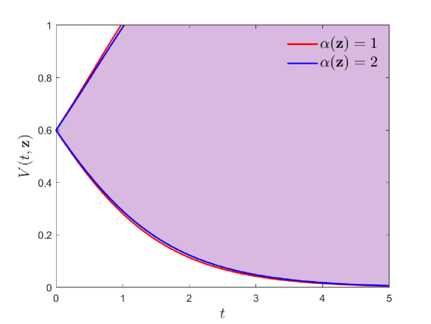
(a) $\rho=0.4$, $\mu(\mathbf{z})=1$

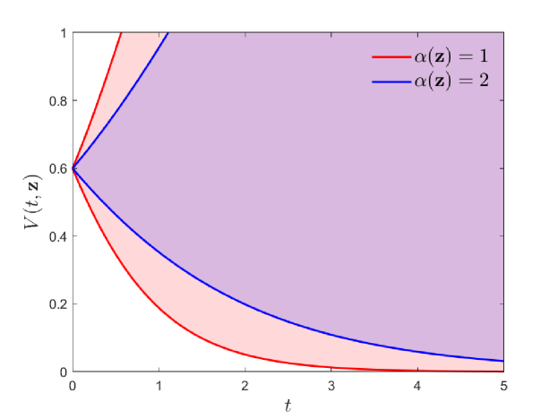
(b) $\rho=0.4$, $\mu(\mathbf{z})=3$

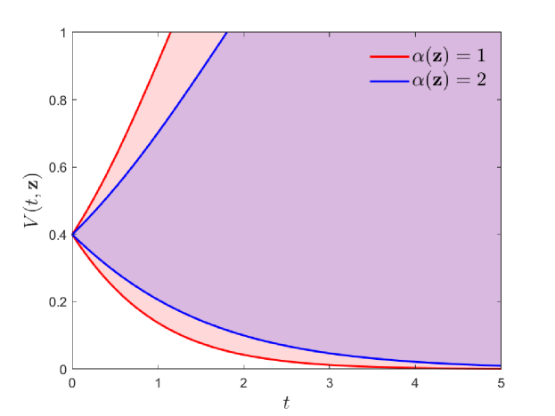
(c) $\rho=0.6$, $\mu(\mathbf{z})=1$

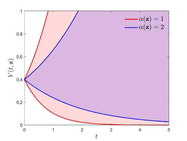
(d) $\rho=0.6$, $\mu(\mathbf{z})=3$

Figure 1: Upper and lower bounds for the time evolution of the mean velocity $V(t,\mathbf{z})$ for $\alpha(\mathbf{z})=1$ (red line) and $\alpha(\mathbf{z})=2$ (blue line), for different values of the traffic density $\rho$ and the parameter $\mu(\mathbf{z})$. The initial velocity is $V_{0}=1-\rho$.

$$\begin{split}&V^{+}(t,\mathbf{z})=\left[\frac{C_{2}(\mathbf{z})}{C_{1}(\mathbf{z})}+e^{-C_{1}(\mathbf{z})t}\left(\frac{1}{V_{0}}-\frac{C_{2}(\mathbf{z})}{C_{1}(\mathbf{z})}\right)\right]^{-1}\\ &V^{-}(t,\mathbf{z})=\left[\frac{C_{2}(\mathbf{z})}{C_{1}(\mathbf{z})}+e^{C_{1}(\mathbf{z})t}\left(\frac{1}{V_{0}}-\frac{C_{2}(\mathbf{z})}{C_{1}(\mathbf{z})}\right)\right]^{-1}\end{split}$$ (20)

and

$$\begin{split}C_{1}(\mathbf{z})=\begin{cases}\frac{\epsilon}{2}(3-P(\rho,\mathbf{z})-P^{2}(\rho,\mathbf{z}))&\beta>0\\ \epsilon P(\rho,\mathbf{z})&\beta\leq 0\end{cases}\\ C_{2}(\mathbf{z})=\begin{cases}\frac{\epsilon}{2}(1+P(\rho,\mathbf{z})-P^{2}(\rho,\mathbf{z}))&\beta>0\\ \frac{\epsilon}{2}(1+P(\rho,\mathbf{z})-P^{2}(\rho,\mathbf{z}))&\beta\leq 0.\end{cases}\end{split}$$ (21)

Let us consider now $\alpha(\mathbf{z})=2$. We define the following constants $C_{1}(\mathbf{z})=\epsilon P(\rho,\mathbf{z})\geq 0$ and $C_{2}(\mathbf{z})=\frac{\epsilon}{2}(P^{2}(\rho,\mathbf{z})+1-P(\rho,\mathbf{z}))>0$ and from (19) we get $V^{-}(t,\mathbf{z})\leq V(t,\mathbf{z})\leq V^{+}(t,\mathbf{z})$ where

$$\begin{split}V^{+}(t,\mathbf{z})&=\left[\frac{C_{1}(\mathbf{z})}{C_{1}(\mathbf{z})+C_{2}(\mathbf{z})}+e^{-(C_{1}(\mathbf{z})+C_{2}(\mathbf{z}))t}\left(\frac{1}{V_{0}}-\frac{C_{1}(\mathbf{z})}{C_{1}(\mathbf{z})+C_{2}(\mathbf{z})}\right)\right]^{-1}\\ V^{-}(t,\mathbf{z})&=\left[\frac{C_{1}(\mathbf{z})}{C_{1}(\mathbf{z})+C_{2}(\mathbf{z})}+e^{(C_{1}(\mathbf{z})+C_{2}(\mathbf{z}))t}\left(\frac{1}{V_{0}}-\frac{C_{1}(\mathbf{z})}{C_{1}(\mathbf{z})+C_{2}(\mathbf{z})}\right)\right]^{-1},\end{split}$$ (22)

with $V(0,\mathbf{z})=V_{0}\in[0,1]$. We point the interested reader to Appendix A for additional details. The impact of the interaction kernel (18) on the introduced traffic model is shown in Figure 1.

As in Section 2.1, the Boltzmann model (17) can be approximated through a surrogate Fokker-Planck model in the quasi-invariant limit. In particular, for the introduced traffic model with interaction kernel we get

$$\begin{split}\partial_{t}f(t,v,\mathbf{z})=&\frac{\sigma^{2}}{2}\partial_{v}^{2}\left[\left(\int_{0}^{1}B(|v-w|,\mathbf{z})f(t,w,\mathbf{z})dw\right)D^{2}(v,\rho)f(t,v,\mathbf{z})\right]\\ &-\partial_{v}\left[\left(\int_{0}^{1}B(|v-w|,\mathbf{z})I(v,w,\mathbf{z})f(t,w,\mathbf{z})dw\right)f(t,v,\mathbf{z})\right],\end{split}$$ (23)

where $I$ has been defined in (15) and $B$ is the interaction kernel as in (18). For the introduced Fokker-Planck equation, at variance with the cases in Sections 3.1-3.2, we cannot compute analytically the equilibrium distribution of the Fokker-Planck model unless $\alpha(\mathbf{z})=0$, corresponding to the Maxwellian scenario.

4 DSMC stochastic Galerkin methods

In this section, we revise the construction of a stochastic Galerkin version of the classical DSMC Algorithm for non-Maxwellian particles, see e.g. [36, 37]. In more detail, we extend the Direct Simulation Monte Carlo stochastic Galerkin (DSMC-sG) methods, introduced in the gas dynamic framework [40], to the models with uncertain parameters proposed in Section 3. Next, we provide consistency results of the DSMC-sG algorithm with respect to relevant observables and in the reconstruction of the kinetic density.

4.1 DSMC-sG for non-Maxwellian models with uncertainties

We first rewrite (2) in strong form to highlight the gain and loss part of the Boltzmann-type equation:

$$\begin{split}\frac{\partial}{\partial t}f(t,v,\mathbf{z})&=Q(f,f)(t,v,\mathbf{z})\\ &=\left\langle\int_{\mathbb{V}}B(v,w,\mathbf{z})\left(\dfrac{1}{J}f(t,{}^{\prime}v,\mathbf{z})f(t,{}^{\prime}w,\mathbf{z})-f(t,v,\mathbf{z})f(t,w,\mathbf{z})\right)dw\right\rangle,\end{split}$$ (24)

where $J$ is the absolute value of the Jacobian of the considered transformation. We denote by $Q_{\Sigma}$ the operator obtained replacing the kernel $B(v,w,\mathbf{z})$ with $B_{\Sigma}(v,w,\mathbf{z})$ given by

$$B_{\Sigma}(v,w,\mathbf{z})=\min\{B(v,w,\mathbf{z}),\Sigma\},$$ (25)

where $\Sigma=\max\{B(v,w,\mathbf{z})\}>0$ is an upper bound for the interaction kernel. By decomposing $Q_{\Sigma}(f,f)$ in its gain and loss part we can rewrite the interaction step as

$$\dfrac{\partial f}{\partial t}(t,v,\mathbf{z})=P(f,f)(t,v,\mathbf{z})-\mu\Sigma f(t,v,\mathbf{z}),$$

with

$$P(f,f)(t,v,\mathbf{z})=Q^{+}_{\Sigma}(f,f)(t,v,\mathbf{z})+f(t,v,\mathbf{z})\left\langle\int_{\mathbb{V}}[\Sigma-B_{\Sigma}(v,w,\mathbf{z})]f(t,w,\mathbf{z})dw\right\rangle,$$

and

$$Q^{+}_{\Sigma}(f,f)=\left\langle\int_{\mathbb{V}}B_{\Sigma}(v,w,\mathbf{z})\dfrac{1}{J}f(t,{}^{\prime}v,\mathbf{z})f(t,{}^{\prime}w,\mathbf{z})dw\right\rangle,$$

with $\mu=\int_{\mathbb{V}}f(t,w,\mathbf{z})dw$.

Let us now consider a time interval $[0,T]$ and let us discretize it in $n_{\textrm{TOT}}$ interval of size $\Delta t>0$. We denote by $f^{n}(v,\mathbf{z})$ the approximation of $f(t^{n},v,\mathbf{z})$ and we consider the forward Euler scheme

$$f^{n+1}=(1-\mu\Sigma\Delta t)f^{n}+\mu\Sigma\Delta t\dfrac{P(f^{n},f^{n})}{\mu\Sigma},$$

where $f^{n+1}$ is a probability density provided $\mu\Sigma\Delta t\leq 1$.

Then, we consider a sample of $N$ particles $v_{i}(\mathbf{z},t)$, $i=1,\dots,N$, from the kinetic solution of the Boltzmann model at time $t$, and we approximate $v_{i}(\mathbf{z},t)$ by its generalized polynomial chaos expansion

$$v_{i}^{M}(\mathbf{z},t)=\sum_{h=0}^{M}\hat{v}_{i,h}(t)\Phi_{h}(\mathbf{z}),$$ (26)

where $\{\Phi_{h}(\mathbf{z})\}_{h=0}^{M}$, $M\in\mathbb{N}$, is a set of orthogonal polynomials of degree less or equal to $M$, orthonormal with respect to the probability density function $p(\mathbf{z})$

$$\int_{I_{\mathbf{z}}}\Phi_{h}(\mathbf{z})\Phi_{k}(\mathbf{z})p(\mathbf{z})d\mathbf{z}=\mathbb{E}_{\mathbf{z}}\left[\Phi_{h}(\cdot)\Phi_{k}(\cdot)\right]=\delta_{hk},\qquad h,k=0,\dots,M,$$ (27)

where $I_{\mathbf{z}}$ is the sample space and $\delta_{hk}$ is the Kronecker delta. The choice for the orthogonal polynomials obviously depends on the distribution of the parameters and follows the so-called Wiener-Askey scheme [50, 51]. In (26), $\hat{v}_{i,h}(t)$ is the projection of the velocity in the subspace generated by the polynomial of degree $h=0,\dots,M$

$$\hat{v}_{i,h}(t)=\int_{I_{\mathbf{z}}}v_{i}(\mathbf{z},t)\Phi_{h}(\mathbf{z})p(\mathbf{z})d\mathbf{z}=\mathbb{E}_{\mathbf{z}}\left[v_{i}(t,\cdot)\Phi_{h}(\cdot)\right].$$ (28)

To perform collision with a non-Maxwellian kernel, we may rewrite the general binary interaction scheme (1) for two particles $v_{i}=v_{i}(\mathbf{z},t)$, $w_{j}=w_{j}(\mathbf{z},t)$, highlighting the acceptance-rejection process introduced by the classical Nanbu-Babovski method [36]

$$\begin{split}&v_{i}^{\prime}(\mathbf{z},t)=v_{i}+\chi\left(\Sigma\xi<B(v_{i},w_{j},\mathbf{z})\right)(\epsilon I_{1}(v_{i},w_{j},\mathbf{z})+D_{1}(v_{i})\eta_{\epsilon})\\ &w_{j}^{\prime}(\mathbf{z},t)=w_{j}+\chi\left(\Sigma\xi<B(v_{i},w_{j},\mathbf{z})\right)(\epsilon I_{2}(v_{i},w_{j},\mathbf{z})+D_{2}(w_{j})\eta_{\epsilon})\end{split}$$ (29)

where $\chi(\cdot)$ is the indicator function and $\xi$ a uniform random number in $(0,1)$. Then, we substitute the velocities $v_{i},\,w_{i}$ with their gPC approximation $v_{i}^{M},\,w_{j}^{M}$ and we project against $\Phi_{h}(\mathbf{z})p(\mathbf{z})d\mathbf{z}$ on $I_{\mathbf{z}}$ for every $h=0,\dots,M$. We obtain

$$\begin{split}&\hat{v}_{i,h}^{\prime}(t)=\hat{v}_{i,h}(t)+\hat{V}^{h}_{i,j}\\ &\hat{w}_{j,h}^{\prime}(t)=\hat{w}_{j,h}(t)+\hat{W}^{h}_{i,j},\end{split}$$ (30)

where $\hat{V}^{h}_{i,j}$, $\hat{W}^{h}_{i,j}$ are the so-called collisional matrices

$$\begin{split}&\hat{V}^{h}_{i,j}=\int_{I_{\mathbf{z}}}\chi\left(\Sigma\xi<B(v^{M}_{i},w^{M}_{j},\mathbf{z})\right)\left((\epsilon I_{1}(v^{M}_{i},w^{M}_{j},\mathbf{z})+D_{1}(v^{M}_{i})\eta_{\epsilon})\right)\Phi_{h}(\mathbf{z})p(\mathbf{z})d\mathbf{z}\\ &\hat{W}^{h}_{i,j}=\int_{I_{\mathbf{z}}}\chi\left(\Sigma\xi<B(v^{M}_{i},w^{M}_{j},\mathbf{z})\right)\left((\epsilon I_{2}(v^{M}_{i},w^{M}_{j},\mathbf{z})+D_{2}(w^{M}_{j})\eta_{\epsilon})\right)\Phi_{h}(\mathbf{z})p(\mathbf{z})d\mathbf{z}.\end{split}$$ (31)

We stress the fact that the new binary interaction for the projections (30) does not depend on the uncertain parameter $\mathbf{z}$. The DSMC-sG method is summarised in Algorithm 1.

Algorithm 1.

(DSMC-sG).

1. compute the initial gPC expansion $\{v_{i}^{M,0},\,i=1,\dots,N\}$ from the initial distribution $f(0,v,\mathbf{z})$;

2. for $n=0$ to $n_{\textrm{TOT}}-1$,
   given the projections $\{\hat{v}_{i,h}^{n},\,i=1,\dots,N,\,h=0,\dots,M\}$:

   • compute an upper bound $\Sigma$ of the kernel;

   • set $N_{c}=\textrm{Sround}(\Sigma\mu\Delta tN/2)$;

   • select $N_{c}$ dummy collision pairs, denoted by $(\hat{v}_{i,h},\,\hat{w}_{j,h})$ with $i=j=1,\dots,N_{c}$, uniformly among all possible pairs and for those:

     • select $\xi$ uniformly in $(0,\,1)$;

     • compute the collision matrices $\hat{V}^{h}_{i,j}$, $\hat{W}^{h}_{i,j}$ (31) for $i,\,j=1,\dots,N_{c},\,h=0,\dots,M$;

     • perform the collision between $i$ and $j$ and compute $\hat{v}^{\prime}_{i,h}$ and $\hat{w}^{\prime}_{j,h}$ according to the collision law (30);

     • set $\hat{v}_{i,h}^{n+1}=\hat{v}^{\prime}_{i,h}$ and $\hat{w}_{j,h}^{n+1}=\hat{w}^{\prime}_{j,h}$;

   • set $\hat{v}_{i,h}^{n+1}=\hat{v}_{i,h}$ and $\hat{w}_{j,h}^{n+1}=\hat{w}_{j,h}$ for all the particles that have not been selected;

   end for,

where by $\textrm{Sround}(x)$ we denote the stochastic rounding of a positive real number $x$

$$\textrm{Sround}=\begin{cases}\lfloor x\rfloor+1&\textrm{with\, probability}\;x-\lfloor x\rfloor\\ \lfloor x\rfloor&\textrm{with\, probability}\;1-x+\lfloor x\rfloor,\end{cases}$$

where $\lfloor x\rfloor$ denotes the integer part of $x$.

4.2 Consistency estimates

We want to evaluate the error produced by the DSMC-sG algorithm in the reconstructed distribution function and its moments. In the following, we denote by $f_{\epsilon}(t,v,\mathbf{z})$ the solution of the Boltzmann equation (3) with binary updates (1) and by $f(t,v,\mathbf{z})$ the corresponding mean field approximation, weak solution of the Fokker-Planck equation (4). We introduce then the empirical density functions

$$f_{\epsilon,N}(t,v,\mathbf{z})=\dfrac{1}{N}\sum_{i=1}^{N}\delta(v-v_{i}(t,\mathbf{z}))\qquad f^{M}_{\epsilon,N}(t,v,\mathbf{z})=\dfrac{1}{N}\sum_{i=1}^{N}\delta(v-v^{M}_{i}(t,\mathbf{z})),$$

where $\delta(\cdot)$ is the Dirac delta function. Being $\varphi$ any test function, we denote by

$$\left\langle\varphi,f_{\epsilon}\right\rangle(\mathbf{z},t)=\int_{\mathbb{V}}f_{\epsilon}(t,v,\mathbf{z})dv$$

its expectation with respect to the distribution function $f_{\epsilon}(t,v,\mathbf{z})$, so that we have

$$\left\langle\varphi,f_{\epsilon,N}\right\rangle(\mathbf{z},t)=\dfrac{1}{N}\sum_{i=1}^{N}\varphi(v_{i}(t,\mathbf{z})),\qquad\left\langle\varphi,f^{M}_{\epsilon,N}\right\rangle(\mathbf{z},t)=\dfrac{1}{N}\sum_{i=1}^{N}\varphi(v^{M}_{i}(t,\mathbf{z})).$$

From the central limit theorem we have the following result [5]

Lemma 1.

If we denote by $\mathbb{E}_{V}[\cdot]$ the expectation with respect to $f_{\epsilon}$ in the velocity space, for each $\mathbf{z}$ the root mean square error satisfies

$${\mathbb{E}_{V}\bigg{[}\Big{(}\left\langle\varphi,f_{\epsilon}\right\rangle(\mathbf{z},t)-\left\langle\varphi,f_{\epsilon,N}\right\rangle(t,\mathbf{z})\Big{)}^{2}\bigg{]}^{1/2}}=\dfrac{\sigma_{\varphi}(t,\mathbf{z})}{N^{1/2}}$$

with

$$\sigma^{2}_{\varphi}(t,\mathbf{z})=\int_{V}{\Big{(}}\varphi(v)-\left\langle\varphi,f_{\epsilon}\right\rangle(t,\mathbf{z}){\Big{)}^{2}}f_{\epsilon}(t,v,\mathbf{z})dv.$$

If $H^{r}(I_{\mathbf{z}})$ is a weighted Sobolev space

$$H^{r}_{p}(I_{\mathbf{z}})=\bigg{\{}v:I_{\mathbf{z}}\rightarrow\mathbb{R}\;:\;\dfrac{\partial^{k}v}{\partial z^{k}}\in L^{2}_{p}(I_{\mathbf{z}}),\;0\leq k\leq r\bigg{\}},$$

from the polynomial approximation theory [50], we have the following spectral estimate

Lemma 2.

For any $v(\mathbf{z})\in H^{r}_{p}(I_{\mathbf{z}}),\,r\geq 0$, there exists a constant $C$ independent of $M>0$ such that

$$\|v-v^{M}\|_{L^{2}_{p}(I_{\mathbf{z}})}\leq\dfrac{C}{M^{r}}\|v\|_{H^{r}_{p}(I_{\mathbf{z}})}.$$

Next, for any random variable $W(\mathbf{z},t)$ taking values in $L^{2}_{p}(I_{\mathbf{z}})$, we define

$$\|W\|_{L^{2}(I_{\mathbf{z}},L^{2}(\mathbb{V}))}=\|\mathbb{E}_{V}[W^{2}]^{1/2}\|_{L^{2}_{p}(I_{\mathbf{z}})},$$

and equivalently

$$\|W\|_{L^{2}(\mathbb{V},L^{2}(I_{\mathbf{z}}))}=\mathbb{E}_{V}\left[\|W\|^{2}_{L^{2}_{p}(I_{\mathbf{z}})}\right]^{1/2},$$

see [16, 40, 38]. Then, we have the following result

Theorem 3.

Let $f(t,v,\mathbf{z})$ be a probability density function, solution of the weak Fokker-Planck equation (4), and $f^{M}_{\epsilon,N}(t,v,\mathbf{z})$ the empirical measure obtained from the $N$-particles sG approximation $\{v^{M}_{i}(\mathbf{z},t)\}_{i}$, solution of the time scaled Boltzmann equation (3). If $v_{i}(\mathbf{z},t)\in H^{r}_{p}(I_{\mathbf{z}})$ for every $i=1,\dots,N$, and in the quasi-invariant limit $\epsilon\rightarrow 0$, we have the following estimate

$$\|\left\langle\varphi,f\right\rangle-\left\langle\varphi,f^{M}_{\epsilon,N}\right\rangle\|_{L^{2}(\mathbb{V},L^{2}_{p}(I_{\mathbf{z}}))}\leq\dfrac{\|\sigma_{\varphi}\|_{L^{2}_{p}(I_{\mathbf{z}})}}{N^{1/2}}+\dfrac{C}{M^{r}}\left(\dfrac{1}{N}\sum_{i=1}^{N}\|\nabla\varphi(\xi_{i})\|_{L^{2}_{p}(I_{\mathbf{z}})}\right),$$

where $\varphi$ is a test function, $C>0$ is a constant independent on $M$ and $\xi_{i}=(1-\theta)v_{i}+\theta v^{M}_{i},\,\theta\in(0,1)$.

Proof.

Thanks to the triangular inequality we have

$$\begin{split}\|\left\langle\varphi,f\right\rangle-\left\langle\varphi,f^{M}_{\epsilon,N}\right\rangle\|_{L^{2}(\mathbb{V},L^{2}_{p}(I_{\mathbf{z}}))}\leq&\underbrace{\|\left\langle\varphi,f\right\rangle-\left\langle\varphi,f_{\epsilon}\right\rangle\|_{L^{2}(\mathbb{V},L^{2}_{p}(I_{\mathbf{z}}))}}_{I}\\ &+\quad\underbrace{\|\left\langle\varphi,f_{\epsilon}\right\rangle-\left\langle\varphi,f_{\epsilon,N}\right\rangle\|_{L^{2}(\mathbb{V},L^{2}_{p}(I_{\mathbf{z}}))}}_{II}\\ &+\quad\underbrace{\|\left\langle\varphi,f_{\epsilon,N}\right\rangle-\left\langle\varphi,f^{M}_{\epsilon,N}\right\rangle\|_{L^{2}(\mathbb{V},L^{2}_{p}(I_{\mathbf{z}}))}}_{III}.\end{split}$$ (32)

In the quasi-invariant regime $\epsilon\rightarrow 0$, up to the extraction of a subsequence, we have

$$\lim_{\epsilon\to 0}f_{\epsilon}(t,v,\mathbf{z})=f(t,v,\mathbf{z}),$$

as a consequence we have

$$\lim_{\epsilon\to 0}\|\left\langle\varphi,f\right\rangle-\left\langle\varphi,f_{\epsilon}\right\rangle\|_{L^{2}(\mathbb{V},L^{2}(I_{\mathbf{z}}))}=0,$$

and the first term vanishes in the quasi-invariant limit. The second term can be evaluated exploiting the result of Lemma 1. Therefore, we have

$$II=\dfrac{\|\sigma_{\varphi}(\mathbf{z})\|_{L^{2}(I_{\mathbf{z}})}}{N^{1/2}}.$$

Finally, we have

$$\left\|\dfrac{1}{N}\sum_{i=1}^{N}\big{(}\varphi(v_{i})-\varphi(v^{M}_{i})\big{)}\right\|_{L^{2}(\mathbb{V},L^{2}_{p}(I_{\mathbf{z}}))}\leq\dfrac{1}{N}\sum_{i=1}^{N}\|\varphi(v_{i})-\varphi(v^{M}_{i})\|_{L^{2}(\mathbb{V},L^{2}_{p}(I_{\mathbf{z}}))},$$

and from the mean value theorem $\varphi(v_{i})-\varphi(v^{M}_{i})=\nabla\varphi(\xi_{i})\cdot(v_{i}-v^{M}_{i})$, for $\xi_{i}=(1-\theta)v_{i}+\theta v^{M}_{i},\,\theta\in(0,1)$. Thanks to Lemma 2 with $C=\max_{i}C_{i}\|v_{i}\|_{H^{r}_{p}(I_{\mathbf{z}})}$ we have

$$III\leq\dfrac{1}{N}\sum_{i=1}^{N}\|\nabla\varphi(\xi_{i})\|_{L^{2}_{p}(I_{\mathbf{z}})}\|v_{i}-v^{M}_{i}\|_{L^{2}_{p}(I_{\mathbf{z}})}\leq\dfrac{C}{M^{r}}\bigg{(}\dfrac{1}{N}\sum_{i=1}^{N}\|\nabla\varphi(\xi_{i})\|_{L^{2}_{p}(I_{\mathbf{z}})}\bigg{)}.$$

∎

Next, we introduce a uniform grid in the domain $\mathbb{V}$, with $\Delta v>0$ width of the cell, and we denote by $S_{\Delta v}\geq 0$ a smoothing function such that

$$\Delta v\int_{\mathbb{V}}S_{\Delta v}(v)dv=1.$$

We consider the approximations of the density function obtained by

$$f_{\epsilon,N,\Delta v}(t,v,\mathbf{z})=\dfrac{1}{N}\sum_{i=1}^{N}S_{\Delta v}(v-v_{i}(t,\mathbf{z}))\qquad f^{M}_{\epsilon,N,\Delta v}(t,v,\mathbf{z})=\dfrac{1}{N}\sum_{i=1}^{N}S_{\Delta v}(v-v^{M}_{i}(t,\mathbf{z})),$$

observing that the standard histogram reconstruction corresponds to the choice $S_{\Delta v}(v)=\chi(|v|\leq\Delta v/2)/\Delta v$. Defining

$$f_{\epsilon,\Delta v}(t,v,\mathbf{z})=\int_{\mathbb{V}}S_{\Delta v}(v-w)f(t,w,\mathbf{z})dw,$$

we have the following result

Theorem 4.

The error introduced by the reconstruction of the distribution in the DSMC-sG method, in the grazing limit $\epsilon\rightarrow 0$, satisfies

$$\begin{split}\|f(t,v,\mathbf{z})-f^{M}_{\epsilon,N,\Delta v}(t,v,\mathbf{z})\|_{L^{2}(\mathbb{V},L^{2}_{p}(I_{\mathbf{z}}))}\leq&\|B_{f_{\epsilon}}\|_{L^{2}_{p}(I_{\mathbf{z}})}(\Delta v)^{q}+\dfrac{\|\sigma_{S_{\Delta v}}\|_{L^{2}_{p}(I_{\mathbf{z}})}}{N^{1/2}}\\ &+\dfrac{C}{M^{r}}\bigg{(}\dfrac{1}{N}\sum_{i=1}^{N}\|\nabla S_{\Delta v}(\xi_{i})\|_{L^{2}_{p}(I_{\mathbf{z}})}\bigg{)},\end{split}$$

where $q>0$, $B_{f_{\epsilon}}>0$ is a constant, $C>0$ is a constant independent on $M$ and $\xi_{i}=(1-\theta)v_{i}+\theta v^{M}_{i},\,\theta\in(0,1)$.

Proof.

Thanks to the triangular inequality we have

$$\begin{split}\|f-f^{M}_{\epsilon,N,\Delta v}\|_{L^{2}(V,L^{2}_{p}(I_{\mathbf{z}}))}\quad&\leq\quad\underbrace{\|f-f_{\epsilon}\|_{L^{2}(V,L^{2}(I_{\mathbf{z}}))}}_{I}\quad+\quad\underbrace{\|f_{\epsilon}-f_{\epsilon,\Delta v}\|_{L^{2}(V,L^{2}_{p}(I_{\mathbf{z}}))}}_{II}\\ &+\quad\underbrace{\|f_{\epsilon,\Delta v}-f_{\epsilon,N,\Delta v}\|_{L^{2}(V,L^{2}_{p}(I_{\mathbf{z}}))}}_{III}\quad+\quad\underbrace{\|f_{\epsilon,N,\Delta v}-f^{M}_{\epsilon,N,\Delta v}\|_{L^{2}(V,L^{2}_{p}(I_{\mathbf{z}}))}}_{IV}.\end{split}$$

In the limit $\epsilon\rightarrow 0$ we have shown that $f_{\epsilon}\rightarrow f$, so the first term vanishes. The second term represents the error introduced by the density reconstruction and is bounded by

$$II\leq\|B_{f_{\epsilon}}\|_{L^{2}_{p}(I_{\mathbf{z}})}(\Delta v)^{q},$$

where $q>0$ depends on the accuracy of the reconstruction. For the last two terms, we observe that

$$f_{\epsilon,\Delta v}=\left\langle\varphi,f_{\epsilon}\right\rangle\qquad f_{\epsilon,N,\Delta v}=\left\langle\varphi,f_{\epsilon,N}\right\rangle\qquad f^{M}_{\epsilon,N,\Delta v}=\left\langle\varphi,f^{M}_{\epsilon,N}\right\rangle$$

with $\varphi(\cdot)=S_{\Delta v}(v-\cdot)$. Hence, we can apply the result of Theorem 3 with the just mentioned choice for $\varphi$. ∎

5 Numerical results

In this section, we present several numerical tests for the DSMC-sG scheme for the non-Maxwellian models with uncertainties described in Section 3. In all the subsequent tests we will consider $N=10^{5}$ agents and the densities are reconstructed through standard histograms.

In more detail, we first check the consistency of the DSMC-sG approximation of the Boltzmann equation with the exact equilibrium distribution for the kinetic model for gambling. Then we test the convergence to the equilibrium of the Fokker-Planck equation for the discussed wealth distribution and the traffic models.

In the binary interactions (29) we introduced the indicator function $\chi(\cdot)$. This term may deteriorate the overall convergence of the DSMC-sG scheme. Coherently with the approach proposed in [40], we introduce the following regularisation

$$\begin{split}&v_{i}^{\prime}(\mathbf{z},t)=v_{i}+K\left(\beta(\Sigma\xi-B(v_{i},w_{j},\mathbf{z}))\right)(\epsilon I_{1}(v_{i},w_{j},\mathbf{z})+D_{1}(v_{i})\eta_{\epsilon})\\ &w_{j}^{\prime}(\mathbf{z},t)=w_{j}+K\left(\beta(\Sigma\xi-B(v_{i},w_{j},\mathbf{z}))\right)(\epsilon I_{2}(v_{i},w_{j},\mathbf{z})+D_{2}(w_{j})\eta_{\epsilon}),\end{split}$$ (33)

where $K(\beta(\cdot))$ is a sigmoid function dependent on the parameter $\beta>0$. In particular, we consider

$$K\left(\beta(\Sigma\xi-B(v_{i},w_{j},\mathbf{z}))\right)=\frac{1}{2}\left(1+\tanh\left(-\beta\left(\Sigma\xi-B(v_{i},w_{j},\mathbf{z})\right)\right)\right).$$ (34)

With this choice, we note that $\beta\gg 1$ is associated with a sharp sigmoid function, on the contrary, a smaller $\beta$ is linked to a smoother sigmoid. We will return to the influence of the parameter $\beta$ in the following.

This regularisation induces a different evolution of the relevant observables. Consequently, to keep the exact time evolution of the first two moments together with the spectral convergence, we couple the DSMC-sG scheme with a scaling process of the form

$$\begin{split}&v_{i}^{\prime\prime}(\mathbf{z},t)=\left(v_{i}^{\prime}(\mathbf{z},t)-V_{K}(t,\mathbf{z})\right)\sqrt{\dfrac{E_{\textrm{FP}}(t,\mathbf{z})}{E_{K}(t,\mathbf{z})}}+V_{\textrm{FP}}(t,\mathbf{z})\\ &w_{j}^{\prime\prime}(\mathbf{z},t)=\left(w_{j}^{\prime}(\mathbf{z},t)-V_{K}(t,\mathbf{z})\right)\sqrt{\dfrac{E_{\textrm{FP}}(t,\mathbf{z})}{E_{K}(t,\mathbf{z})}}+V_{\textrm{FP}}(t,\mathbf{z}),\end{split}$$ (35)

where $V_{\textrm{FP}}(t,\mathbf{z})$ and $E_{\textrm{FP}}(t,\mathbf{z})$ are, respectively, the mean velocity and the energy computed from the corresponding surrogate Fokker-Planck model. Similarly, we indicated with $V_{K}(t,\mathbf{z})$ and $E_{K}(t,\mathbf{z})$ mean velocity and energy of the Boltzmann-type model with sigmoid function $K(\cdot)$ (34) in equation (33). The computation of $V_{\textrm{FP}}(t,\mathbf{z})$ and $E_{\textrm{FP}}(t,\mathbf{z})$ follows from the model (4) that is solved through standard sG method and for which we can guarantee sufficient regularity under the assumptions of Theorem 2. We highlight how the additional scaling process (35) will be consistent with the original Boltzmann-type model in the regime $\epsilon\ll 1$.

For clarity purposes, in the rest of the section we will indicate the numerical solution of the Fokker-Planck model $f_{\textrm{FP}}(t,v,\mathbf{z})$ and the numerical solution of the Boltzmann-type model as $f_{\epsilon}(t,v,\mathbf{z})$, whereas the solution of the Boltzmann-type model with additional scaling process (35) will be denoted by $\tilde{f}_{\epsilon}(t,v,\mathbf{z})$. For the approximation of the Fokker-Planck model we will implement a standard sG collocation method based on a semi-implicit scheme presented in [39] and further studied in [17, 48, 52].

5.1 Test 1: gambling

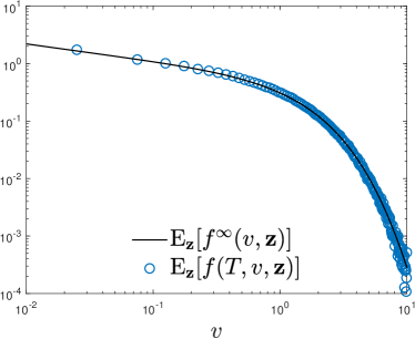
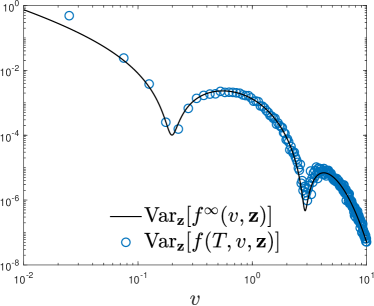
Figure 2: Test 1. Comparison of $f^{\infty}(v,\mathbf{z})$ in (37) and DSMC-sG approximation of $f(T,v,\mathbf{z})$ at time $T=10$, in log-log scale, in terms of expectation (left) and variance (right) with respect to uncertain parameter $\delta(z)=\frac{1}{2}z$, $z\sim\mathcal{U}([0,1])$. We consider $N=10^{5}$ particles with $M=5$ Galerkin projections, time step $\Delta t=0.1$ and initial density (36).

We consider the kinetic model for gambling with 1D uncertainty in the collisional kernel. We choose $\delta(z)=\frac{1}{2}z$ and $z\sim\mathcal{U}([0,1])$ in (9) fixing $\kappa=1$. Since the random parameter is uniformly distributed, we use the Legendre polynomials in the gPC expansion. In all the simulations, we consider $M=5$ Galerkin projections and the time frame $[0,T]$ with $T=10$ discretised with time step $\Delta t=0.1$. The kinetic density is reconstructed in the interval $[0,10]$ with $\Delta v=0.05$. We consider the deterministic initial distribution

$$f(0,v,\mathbf{z})=\begin{cases}\dfrac{1}{2}&v\in[0,2]\\ 0&\textrm{elsewhere}.\end{cases}$$ (36)

In this test, we highlight that the equilibrium solution of the Boltzmann-type model can be computed exactly and $\epsilon=1$ and reads

$$f^{\infty}(v,\mathbf{z})=\dfrac{(1-\delta)^{1-\delta}}{\Gamma(1-\delta)}v^{-\delta}\exp\{-(1-\delta)v\},$$ (37)

see Section 3.1. In Figure 2, we report expected value and variance with respect to the random parameter $z$ of the DSMC-sG approximation. We may observe the good agreement of the considered quantities of interest with the analytical ones.

5.2 Test 2: wealth distribution

We consider now the kinetic model for the wealth distribution described in Section 3.2. In particular, we consider the case where the interaction kernel (11) is characterized by $\delta(\mathbf{z})=\mathbf{z}\sim\mathcal{U}([0,1])$ and $\kappa=1$. Therefore, we adopt the Legendre polynomials in the gPC expansion of the velocities. In all the results of this test, we consider a background uniformly distributed as $\mathcal{E}\sim\mathcal{U}([0.9,1.1])$. Furthermore, we consider the following deterministic initial distribution

$$f(0,v,\mathbf{z})=\begin{cases}\dfrac{1}{2}&v\in[0,2]\\ 0&\textrm{elsewhere}.\end{cases}$$ (38)

In Figure 3 we show expectation and variance of $f_{\epsilon}(t,v,\mathbf{z})$ computed through DSMC-sG method with respect to the analytical equilibrium distribution of the Fokker-Planck model (14), for various $\epsilon=5\times 10^{-2},10^{-1},5\times 10^{-1}$. In the last picture we report also the behavior of the expected mean wealth $\mathbb{E}_{\mathbf{z}}[V_{\epsilon}(t,\mathbf{z})]$ for the introduced values of $\epsilon$. We consider $M=5$ Galerkin projections, $\Delta t=\epsilon/10$, $\lambda=\sigma^{2}=0.5$ and time frame $[0,T]$ with $T=10$. The kinetic density is reconstructed through standard histogram over the interval $[0,10]$ with $\Delta v=0.05$.

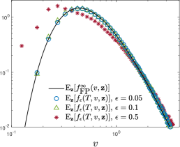
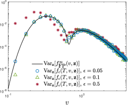
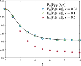
Figure 3: Test 2. Comparison of $f^{\infty}_{\textrm{FP}}(v,\mathbf{z})$ and the DSMC-sG approximation of $f_{\epsilon}(T,v,\mathbf{z})$ at time $T=10$, in log-log scale, in terms of expectation (left) and variance (center) for several $\epsilon=5\times 10^{-2},10^{-1},5\times 10^{-1}$. We report (right) the time evolution of $\mathbb{E}_{\mathbf{z}}[V_{\epsilon}(t,\mathbf{z})]$ for several $\epsilon$ and $\mathbb{E}_{\mathbf{z}}[V_{\textrm{FP}}(t,\mathbf{z})]$. We consider $N=10^{5}$ particles with $M=5$ Galerkin projections and $\Delta t=\epsilon/10$. The random parameter is uniformly distributed $\delta(\mathbf{z})=\mathbf{z}\sim\mathcal{U}([0,1])$, and we fix $\kappa=1$, $\lambda=\sigma^{2}=0.5$. The background $\mathcal{E}$ is a uniform distribution $\mathcal{U}([0.9,1.1])$.

In order to show spectral convergence property of the scheme, we consider a reference DSMC-sG evolution of $E_{\epsilon}(t,\mathbf{z})$ obtained with $\epsilon=0.1$, $N=10^{5}$, $\Delta t=0.1$ and sG scheme up to order $M=50$. We store the collisional tree generating the reference solution and we check the $L^{2}$ convergence of the scheme. In Figure (4) we present the decay of the $L^{2}$ error for increasing $M$ obtained from the initial distribution (38). If we consider the original binary dynamics (29), even if the expectation is well described, it can be observed that the spectral accuracy of the method is lost due to discontinuity of the indicator function $\chi(\cdot)$. The same test performed for the binary dynamics (33) recovers spectral accuracy. For increasing $\beta\gg 0$ the convergence of the scheme is deteriorated, since we approximate a step function.

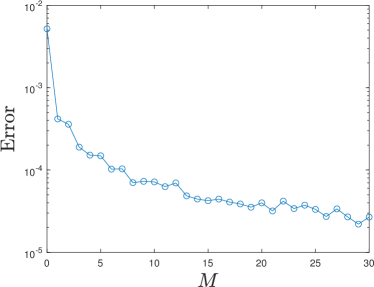
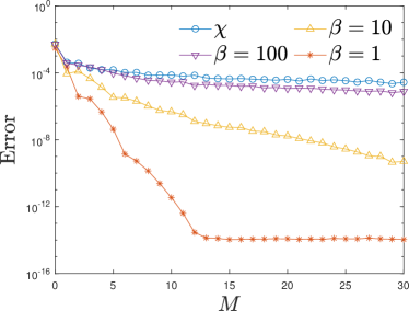
Figure 4: Test 2. Convergence of the $L^{2}$ error of the DSMC-sG scheme, where the binary interaction dynamics are given by (29) (left) or by (33) (right), in the case of model for wealth distribution with uncertain kernel. We consider $N=10^{5}$, $\Delta t=0.01$ and $\epsilon=0.1$. We fix $\kappa=1$, $\lambda=\sigma^{2}=0.5$. Reference solution computed with $M=50$.

Coupling now (33) with the process (35), we recover qualitatively consistent approximation of the evolution of relevant quantities of interest together with spectral convergence for moderate values of $\beta>0$, see Figure 5. In this test we solve the Fokker-Planck model (13).

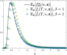
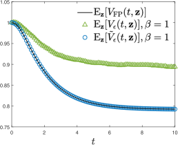
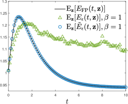
Figure 5: Test 2. Left: comparison of $f^{\infty}_{\textrm{FP}}$ in (14) with the DSMC-sG approximation of $f_{\epsilon}(t,v,\mathbf{z})$ (regularization without rescaling) and of $\tilde{f}_{\epsilon}(t,v,\mathbf{z})$ (regularization with rescaling), in terms of expectation in $\mathbf{z}$. Center and right: comparison of $V_{\textrm{FP}},E_{\textrm{FP}}$ with the DSMC-sG approximation of $V_{\epsilon}(t,\mathbf{z}),E_{\epsilon}(t,\mathbf{z})$ (regularization without rescaling) and of $\tilde{V}_{\epsilon}(t,\mathbf{z}),\tilde{E}_{\epsilon}(t,\mathbf{z})$ (regularization with rescaling). We consider $N=10^{5}$, $M=5$, $\Delta t=0.01$ and $\epsilon=0.1$. We fix $\kappa=1$, $\lambda=\sigma^{2}=0.5$

5.3 Test 3: traffic flow

In this last test, we consider the traffic model of Section 3.3, affected by an uncorrelated 2D random parameter $\mathbf{z}=(z_{1},z_{2})$ with $p(\mathbf{z})=p_{1}(z_{1})p_{2}(z_{2})$. In particular, we consider $z_{1}$ affecting $\mu(z_{1})$ in the interaction function $I(v,w,z_{1})$ defined in (15) and $z_{2}$ affecting $\alpha(z_{2})$ in the kernel $B(|v-w|,z_{2})$ defined in (18). Under these assumptions, the gPC expansion of the velocities $v_{i}(t,z_{1},z_{2})$, $i=1,\dots,N$ reads

$$v_{i}^{M_{1},M_{2}}(z_{1},z_{2},t)=\sum_{h=0}^{M_{1}}\sum_{k=0}^{M_{2}}\hat{v}_{i,h,k}(t)\Phi^{(1)}_{h}(z_{1})\Phi^{(2)}_{k}(z_{2}),$$ (39)

being $\{\Phi^{(1)}_{h}(z_{1})\}_{h=0}^{M_{1}}$ and $\{\Phi^{(2)}_{k}(z_{2})\}_{k=0}^{M_{2}}$ the polynomials orthogonal with respect to the distributions $p_{1}(z_{1})$ and $p_{2}(z_{2})$, respectively. Substituting $v_{i}^{M_{1},M_{2}}(z_{1},z_{2},t)$ into the binary interaction (16) and and proceeding as in Section 4.1, we obtain

$$\begin{split}&\hat{v}_{i,h,k}^{\prime}(t)=\hat{v}_{i,h,k}(t)+\hat{V}^{h,k}_{i,j}\\ &\hat{w}_{j,h,k}^{\prime}(t)=\hat{w}_{j,h,k}(t),\end{split}$$ (40)

with the following collision matrix

$$\begin{split}\hat{V}^{h,k}_{i,j}=&\int_{I_{\mathbf{z}}}\chi\left(\Sigma\xi<B(v_{i}^{M_{1},M_{2}},w_{j}^{M_{1},M_{2}},z_{2})\right)\\ &\left(\gamma I(v_{i}^{M_{1},M_{2}},w_{j}^{M_{1},M_{2}},z_{1})+D(v_{i}^{M_{1},M_{2}};\rho)\eta\right)\Phi^{(1)}_{h}(z_{1})\Phi^{(2)}_{k}(z_{2})p_{1}(z_{1})p_{2}(z_{2})dz_{1}dz_{2}.\end{split}$$ (41)

We consider the following deterministic initial distribution

$$f(0,v,\mathbf{z})=\begin{cases}1&v\in[0,1]\\ 0&\textrm{elsewhere}.\end{cases}$$ (42)

To assess the impact of the single uncertain parameters on the dynamics we first consider the case $\mu(z_{1})=1+2z_{1}$ and $\alpha(z_{2})=2z_{2}$ with uncorrelated uncertainties $z_{1},z_{2}\sim\mathcal{U}([0,1])$. In Figure 6 we show the DSMC-sG approximation of the solution of Fokker-Planck model for traffic (23) in terms of expected value and variance in $\mathbf{z}=(z_{1},z_{2})$ of the distribution function and of the macroscopic quantities. We considered two different densities $\rho=0.4$ and $\rho=0.6$ and the Fokker-Planck is solved on a grid of $N_{v}=51$ points such that $\Delta v=0.02$ and $\Delta t=\Delta v/2$. As before, the DSMC-sG provides a good approximation in the limit $\epsilon\ll 1$ of the solution of the Fokker-Planck model.

We show the $L^{2}$ convergence of the DSMC-sG scheme in Figure 7. In details, we considered the case with binary interactions (29) in the left plot, whereas the case with regularization of the step function as in (33), with $\beta=0.01$, is presented in the right plot. The error has been computed with respect to a reference DSMC-sG evolution of $E_{\epsilon}(t,\mathbf{z})$ with $\Delta t=\epsilon=0.1$, $N=10^{5}$, and $M_{1}=M_{2}=50$. As before, in this test we store the collisional tree of the reference solution and we check $L^{2}$ convergence for increasing $M_{1},M_{2}$. The error is presented here in $\log_{10}$ and we can clearly observe spectral accuracy in the case with regularization.

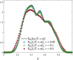
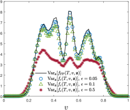
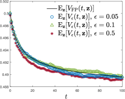
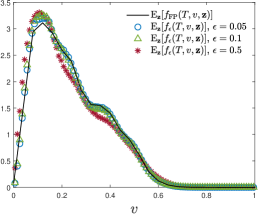
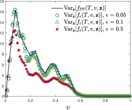
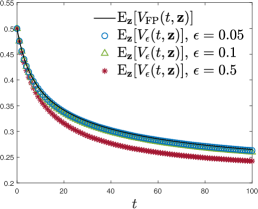
Figure 6: Test 3. Comparison of the numerical solution of the Fokker-Planck model (23) with $\mu(z_{1})=1+2z_{1}$ and $\alpha(z_{2})=2z_{2}$, $z_{1},z_{2}\sim\mathcal{U}([0,1])$, with the DSMC-sG reconstruction of traffic distributions (first and second column) and of mean velocity (third column) for various $\epsilon=0.05,0.1,0.5$. We considered $\rho=0.4$ (top row) and $\rho=0.6$ (bottom row). We set for the DSMC-sG method $N=10^{5}$, $M_{1}=M_{2}=5$, $\Delta t=\epsilon$, and the deterministic solver for Fokker-Planck is such that $\Delta v=0.02$ and $\Delta t=\Delta v/2$. The time frame is $t\in[0,T]$, $T=300$.

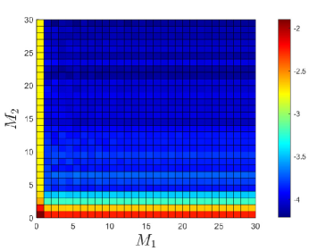
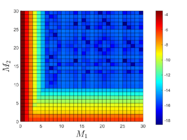
Figure 7: Test 3. Convergence of the $L^{2}$ error of the DSMC-sG scheme where binary dynamics are given by (29) (left) or by (33) where $\beta=0.01$, in the case of model for traffic flow with 2D uncorrelated uncertainty in interactions and kernel. We consider $N=10^{5}$, $\Delta t=\epsilon=0.1$. We fix $\rho=0.4$, $\mu(z_{1})=1+2z_{1}$ and $\alpha(z_{2})=2z_{2}$ with $z_{1},z_{2}\sim\mathcal{U}([0,1])$. Reference solution computed with $M_{1}=M_{2}=50$.

Finally, coupling (33) with the process (35), we recover a qualitatively consistent approximation of the evolution of relevant quantities of interest in the case of traffic flow model, see Figure 8.

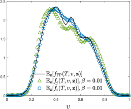
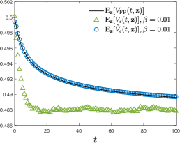
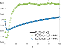
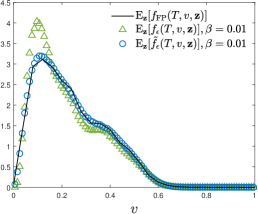
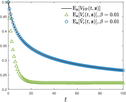
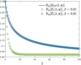
Figure 8: Test 3. First column: comparison of numerical $f_{\textrm{FP}}(T,v,\mathbf{z})$ with the DSMC-sG approximation of $f_{\epsilon}(T,v,\mathbf{z})$ (regularization without rescaling) and of $\tilde{f}_{\epsilon}(T,v,\mathbf{z})$ (regularization with rescaling) in terms of the expectation in $\mathbf{z}$. Central and right columns: comparison of $V_{\textrm{FP}}$, $E_{\textrm{FP}}$ with the DSMC-sG approximation without rescaling $V_{\epsilon}(t,\mathbf{z})$, $E_{\epsilon}(t,\mathbf{z})$ and with rescaling $\tilde{V}_{\epsilon}(t,\mathbf{z})$, $\tilde{E}_{\epsilon}(t,\mathbf{z})$. Top row: $\rho=0.4$, bottom row: $\rho=0.6$. We consider $N=10^{5}$, $M_{1}=M_{2}=5$ and $\Delta t=\epsilon=0.1$.

Conclusion

In this work, we studied an extension of a recently introduced DSMC-sG hybrid approach [8, 40] for uncertainty quantification of kinetic equations to non-Maxwellian Boltzmann-type models for multi-agent systems. The proposed method combines a DSMC solver in the physical space with a stochastic Galerkin method in the random space and is based on a generalized Polynomial Chaos expansion of statistical samples of a DSMC solver. The DSMC-sG solution of non-Maxwellian models with uncertainties requires a suitable reformulation of classical DSMC solvers. The class of kinetic models of interest can be formally approximated by surrogate Fokker-Planck-type models in the quasi-invariant regime. For these models, the regularity in the random space has been investigated. In particular, exploiting this observation we guarantee spectral accuracy of the method in the random space. Several examples based on existing models of multi-agent systems have been investigated numerically. The extension of the DSMC-sG methods to non-homogeneous equations of collective phenomena is currently under investigation.

Competing interests

The authors declare no competing interests.

Data availability statement

The dataset generated during the current study is available from the corresponding author on reasonable request.

Appendix A Non-Maxwellian traffic model

Let us consider first the case $\alpha(\mathbf{z})=1$. From (19) we have

$$\begin{split}\left|\frac{1}{\epsilon}\frac{dV(t,\mathbf{z})}{dt}\right|&\leq\underbrace{\left|\int_{0}^{1}\int_{0}^{v}(v-w)I(v,w,\mathbf{z})f(t,v,\mathbf{z})f(t,w,\mathbf{z})dwdv\right|}_{A}\\ &\quad+\underbrace{\dfrac{1}{2}\left|\int_{0}^{1}\int_{0}^{1}(w-v)I(v,w,\mathbf{z})f(t,v,\mathbf{z})f(t,w,\mathbf{z})dwdv\right|.}_{B}\end{split}$$ (43)

In particular, a direct integration of the second term gives

$$B=\dfrac{1}{2}(E(t,\mathbf{z})-V^{2}(t,\mathbf{z}))(P(\rho,\mathbf{z})-P^{2}(\rho,\mathbf{z})+1)>0$$

being $P\in[0,1]$ for all $\mathbf{z}$ and where $E(t,\mathbf{z})=\int_{0}^{1}v^{2}f(t,v,\mathbf{z})dv$ is the energy. On the other hand, thanks to triangular inequality, we have

$$\begin{split}&A\leq\underbrace{\int_{0}^{1}\int_{0}^{v}(v-w)|P(\rho,\mathbf{z})(1-v)|f(t,v,\mathbf{z})f(t,w,\mathbf{z})dwdv}_{\textrm{A}_{1}}\\ &\quad+\underbrace{\int_{0}^{1}\int_{0}^{v}(v-w)|(1-P(\rho,\mathbf{z}))(P(\rho,\mathbf{z})w-v)|f(t,v,\mathbf{z})f(t,w,\mathbf{z})dwdv.}_{\textrm{A}_{2}}\end{split}$$ (44)

Since $P\geq 0$ and $v\in[0,1]$ we have

$$\begin{split}\textrm{A}_{1}&=\int_{0}^{1}P(\rho,\mathbf{z})(1-v)\left[\int_{0}^{v}(v-w)f(t,w,\mathbf{z})dw\right]f(t,v,\mathbf{z})dv\\ &\leq\int_{0}^{1}P(\rho,\mathbf{z})(1-v)vf(t,v,\mathbf{z})dv=P(\rho,\mathbf{z})(V(t,\mathbf{z})-E(t,\mathbf{z})).\end{split}$$

Similarly, for the second term of (44) we have

$$\begin{split}\textrm{A}_{2}&=\int_{0}^{1}\int_{0}^{v}(v-w)(1-P(\rho,\mathbf{z}))vf(t,v,\mathbf{z})f(t,w,\mathbf{z})dwdv\\ &\leq\int_{0}^{1}(1-P(\rho,\mathbf{z}))v^{2}f(t,v,\mathbf{z})dv=(1-P(\rho,\mathbf{z}))E(t,\mathbf{z}),\end{split}$$

From the obtained inequalities we conclude that

$$\begin{split}\left|\frac{dV(t,\mathbf{z})}{dt}\right|\leq&\frac{\epsilon}{2}\Big{[}2P(\rho,\mathbf{z})V(t,\mathbf{z})-V^{2}(t,\mathbf{z})(P(\rho,\mathbf{z})-P^{2}(\rho,\mathbf{z})+1)\\ &+E(t,\mathbf{z})(3-3P(\rho,\mathbf{z})-P^{2}(\rho,\mathbf{z}))\Big{]}.\end{split}$$ (45)

Since $v\in[0,1]$ we have $E(t,\mathbf{z})\leq V(t,\mathbf{z})$ and, introducing the notation $\beta(\mathbf{z})=3-3P(\rho,\mathbf{z})-P^{2}(\rho,\mathbf{z})$, we get

$$\begin{cases}\left|\dfrac{dV(t,\mathbf{z})}{dt}\right|\leq\frac{\epsilon}{2}\left[V(t,\mathbf{z})(3-P(\rho,\mathbf{z})-P^{2}(\rho,\mathbf{z}))-V^{2}(t,\mathbf{z})(P(\rho,\mathbf{z})-P^{2}(\rho,\mathbf{z})+1)\right]&\beta>0\\ \left|\dfrac{dV(t,\mathbf{z})}{dt}\right|\leq\frac{\epsilon}{2}\left[2V(t,\mathbf{z})P(\rho,\mathbf{z})-V^{2}(t,\mathbf{z})(P(\rho,\mathbf{z})-P^{2}(\rho,\mathbf{z})+1)\right]&\beta\leq 0,\end{cases}$$

that are both Bernoulli-type ODEs.

Hence, we get $V^{-}(t,\mathbf{z})\leq V(t,\mathbf{z})\leq V^{+}(t,\mathbf{z})$ where

$$\begin{split}&V^{+}(t,\mathbf{z})=\left[\frac{C_{2}(\mathbf{z})}{C_{1}(\mathbf{z})}+e^{-C_{1}(\mathbf{z})t}\left(\frac{1}{V_{0}}-\frac{C_{2}(\mathbf{z})}{C_{1}(\mathbf{z})}\right)\right]^{-1}\\ &V^{-}(t,\mathbf{z})=\left[\frac{C_{2}(\mathbf{z})}{C_{1}(\mathbf{z})}+e^{C_{1}(\mathbf{z})t}\left(\frac{1}{V_{0}}-\frac{C_{2}(\mathbf{z})}{C_{1}(\mathbf{z})}\right)\right]^{-1}\end{split}$$ (46)

where

$$\begin{split}\begin{cases}C_{1}(\mathbf{z})=\frac{\epsilon}{2}(3-P(\rho,\mathbf{z})-P^{2}(\rho,\mathbf{z}))&\beta>0\\ C_{1}(\mathbf{z})=\epsilon P(\rho,\mathbf{z})&\beta\leq 0\end{cases}\\ \begin{cases}C_{2}(\mathbf{z})=\frac{\epsilon}{2}(1+P(\rho,\mathbf{z})-P^{2}(\rho,\mathbf{z}))&\beta>0\\ C_{2}(\mathbf{z})=\frac{\epsilon}{2}(1+P(\rho,\mathbf{z})-P^{2}(\rho,\mathbf{z}))&\beta\leq 0.\end{cases}\end{split}$$ (47)

Hence, we consider the case $\alpha(\mathbf{z})=2$. We define the following constants $C_{1}(\mathbf{z})=\epsilon P(\rho,\mathbf{z})\geq 0$ and $C_{2}(\mathbf{z})=\frac{\epsilon}{2}(P^{2}(\rho,\mathbf{z})+1-P(\rho,\mathbf{z}))>0$ and from (19) we get

$$\frac{dV(t,\mathbf{z})}{dt}=C_{1}(\mathbf{z})\left(E(t,\mathbf{z})-V^{2}(t,\mathbf{z})\right)+C_{2}(\mathbf{z})\left(E(t,\mathbf{z})V(t,\mathbf{z})-M_{3}(t,\mathbf{z})\right),$$ (48)

where $M_{3}(t,\mathbf{z})=\int_{0}^{1}v^{3}f(t,v,\mathbf{z})dv$. Hence, from the triangular inequality we find

$$\left|\frac{dV(t,\mathbf{z})}{dt}\right|\leq C_{1}(\mathbf{z})\left(E(t,\mathbf{z})-V^{2}(t,\mathbf{z})\right)+C_{2}(\mathbf{z})\left|E(t,\mathbf{z})V(t,\mathbf{z})-M_{3}(t,\mathbf{z})\right|.$$ (49)

Arguing as before, we get

$$\begin{split}C_{1}(\mathbf{z})\left(E(t,\mathbf{z})-V^{2}(t,\mathbf{z})\right)&\leq C_{1}(\mathbf{z})\left(V(t,\mathbf{z})-V^{2}(t,\mathbf{z})\right),\\ C_{2}(\mathbf{z})\left|E(t,\mathbf{z})V(t,\mathbf{z})-M_{3}(t,\mathbf{z})\right|&\leq C_{2}(\mathbf{z})V(t,\mathbf{z}).\end{split}$$ (50)

Therefore we get $V^{-}(t,\mathbf{z})\leq V(t,\mathbf{z})\leq V^{+}(t,\mathbf{z})$ where

$$\begin{split}V^{+}(t,\mathbf{z})&=\left[\frac{C_{1}(\mathbf{z})}{C_{1}(\mathbf{z})+C_{2}(\mathbf{z})}+e^{-(C_{1}(\mathbf{z})+C_{2}(\mathbf{z}))t}\left(\frac{1}{V_{0}}-\frac{C_{1}(\mathbf{z})}{C_{1}(\mathbf{z})+C_{2}(\mathbf{z})}\right)\right]^{-1}\\ V^{-}(t,\mathbf{z})&=\left[\frac{C_{1}(\mathbf{z})}{C_{1}(\mathbf{z})+C_{2}(\mathbf{z})}+e^{(C_{1}(\mathbf{z})+C_{2}(\mathbf{z}))t}\left(\frac{1}{V_{0}}-\frac{C_{1}(\mathbf{z})}{C_{1}(\mathbf{z})+C_{2}(\mathbf{z})}\right)\right]^{-1},\end{split}$$ (51)

with $V(0,\mathbf{z})=V_{0}\in[0,1]$.

References

- [1] H. Babovsky and R. Illner. A convergence proof for nanbu’s simulation method for the full boltzmann equation. SIAM J. Numer. Anal., 26:45–65, 1989.
- [2] H. Babovsky and H. Neunzert. On a simulation scheme for the boltzmann equation. Math. Meth. Appl. Sci., 8:223–233, 1986.
- [3] F. Bassetti and G. Toscani. Explicit equilibria in a kinetic model of gambling. Phys. Rev. E, 81:066115, 2010.
- [4] G. Bertaglia, L. Liu, L. Pareschi, and X. Zhu. Bi-fidelity stochastic collocation methods for epidemic transport models with uncertainties. Netw. Heterog. Media, in press.
- [5] R. E. Caflisch. Monte Carlo and quasi Monte Carlo methods. Acta numerica, 7:1–49, 1998.
- [6] J. A. Carrillo, M. R. D’Orsogna, and V. Panferov. Double milling in self-propelled swarms from kinetic theory. Kinetic. Relat. Models, 2(2):363–378, 2009.
- [7] J. A. Carrillo, M. Fornasier, J. Rosado, and G. Toscani. Asymptotic flocking dynamics for the kinetic Cucker-Smale model. SIAM J. Math. Anal., 42(1):218–236, 2010.
- [8] J. A. Carrillo, L. Pareschi, and M. Zanella. Particle based gPC methods for mean-field models of swarming with uncertainty. Commun. Comput. Phys., 25(2):508–531, 2019.
- [9] C. Cercignani, R. Illner, and M. Pulvirenti. The Mathematical Theory of Dilute Gases, volume 106 of Applied Mathematical Sciences. Springer, 1994.
- [10] Y.-P. Choi and S.-B. Yun. Existence and hydrodynamic limit for a Paveri-Fontana type kinetic traffic model. SIAM J. Math. Anal., 53:2631–2659, 2021.
- [11] S. Cordier, L. Pareschi, and G. Toscani. On a kinetic model for a simple market economy. J. Stat. Phys., 120(1):253–277, 2005.
- [12] P. Degond and S. Motsch. Continuum limit of self-driven particles with orientation interaction. Math. Models Meth. Appl. Sci., 18(supp01):1193–1215, 2008.
- [13] L. Desvillettes. Boltzmann’s kernel and the spatially homogeneous Boltzmann equation. Riv. Mat. Univ. Parma, 6(4):1–22, 2001.
- [14] G. Dimarco and L. Pareschi. Numerical methods for kinetic equations. Acta Numerica, 23:369–520, 2014.
- [15] G. Dimarco and L. Pareschi. Multi-scale control variate methods for uncertainty quantification in kinetic equations. J. Comp. Phys., 388:63–89, 2019.
- [16] G. Dimarco and L. Pareschi. Multiscale variance reduction methods based on multiple control variates for kinetic equations with uncertainties. Multiscale Model. Simul., 18(1):351–382, 2020.
- [17] G. Dimarco, L. Pareschi, and M. Zanella. Uncertainty quantification for kinetic models in socio-economic and life sciences. In S. Jin and L. Pareschi, editors, Uncertainty quantification for Hyperbolic and Kinetic Equations, volume 14 of SEMA-SIMAI Springer Series, pages 151–191. Springer, 2017.
- [18] G. Dimarco, B. Perthame, G. Toscani, and M. Zanella. Kinetic models for epidemic dynamics with social heterogeneity. J. Math. Biol., 83(4), 2021.
- [19] A. Dragulescu and V. M. Yakovenko. Statistical mechanics of money. Eur. Phys. J. B, 17:723–729, 2000.
- [20] B. Düring, M. Fischer, and M.-T. Wolfram. An Elo-type rating model for players and teams of variable strength. Philos. Trans. R. Soc. Lond. Ser. A Phys. End. Sci., 2021.
- [21] B. Düring, M. Torregrossa, and M.-T. Wolfram. Boltzmann and Fokker-Planck equations modelling the Elo rating system with learning effects. J. Nonlinear Sci., 29(3):1095–1128, 2019.
- [22] B. Düring and M.-T. Wolfram. Opinion dynamics: inhomogeneous Boltzmann-type equations modelling opinion leadership and political segregation. Proc. R. Soc. A, 417(2182), 2015.
- [23] G. Furioli, A. Pulvirenti, E. Terraneo, and G. Toscani. Non-Maxwellian kinetic equations modelling the evolution of wealth distribution. Math. Models Meth. Appl. Sci., 30(4):685–725, 2020.
- [24] I. Gamba, S. Jin, and L. Liu. Error estimate of a bi-fidelity method for kinetic equations with random parameters and multiple scales. Int. J. Uncertain. Quantif., 11(5):57–75, 2021.
- [25] D. Helbing. Gas-kinetic derivation of Navier-Stokes-like traffic equations. Phys. Rev. E, 53(3):2366–2381, 1996.
- [26] M. Herty, A. Klar, and L. Pareschi. General kinetic models for vehicular traffic flow and Monte Carlo methods. Comput. Meth. Appl. Math., 5:155–169, 2005.
- [27] M. Herty and L. Pareschi. Fokker-Planck asymptotics for traffic flow models. Kinet. Relat. Mod., 3(1):165–179, 2010.
- [28] J. Hu, S. Jin, and R. Shu. On stochastic galerkin approximation of the nonlinear Boltzmann equation with uncertainty in the fluid regime. J. Comp. Phys., 397:108838, 2019.
- [29] J. Hu, L. Pareschi, and Y. Wang. Uncertainty quantification for the BGK model of the boltzmann equation using multilevel variance reduced monte carlo methods. SIAM/ASA J. Uncert. Quantif., 9(2):650–680, 2021.
- [30] S. Jin, J. G. Liu, and Z. Ma. Uniform spectral convergence of the stochastic galerkin method for the linear transport equations with random inputs in diffusive regime and a micro–macro decomposition-based asymptotic-preserving method. Res. Math. Sci., 4(15), 2017.
- [31] S. Jin and L. Pareschi, editors. Uncertainty quantification for hyperbolic and kinetic equations, volume 14 of SEMA-SIMAI Springer Series. Springer, 2017.
- [32] M. Kac. Probability and Related Topics in the Physical Sciences. New York Interscience, 1959.
- [33] Q. Li and L. Wang. Uniform regularity for linear kinetic equations with random input based on hypocoercivity. SIAM/ASA J. Uncert. Quantif., 5(1):1193–1219, 2017.
- [34] L. Liu and S. Jin. Hypocoercivity based sensitivity analysis and spectral convergence of the stochastic Galerkin approximation to collisional kinetic equations with multiple scales and random inputs. Multiscale Model. Simul., 16(3):1085–1114, 2018.
- [35] K. Nanbu. Direct simulation scheme derived from the Boltzmann equation. i. monocomponent gases. J. Phys. Soc. Jpn., 49:2042–2049, 1980.
- [36] L. Pareschi and G. Russo. An introduction to Monte Carlo methods for the Boltzmann equation. ESAIM: Proc., 10:35–75, 2001.
- [37] L. Pareschi and G. Toscani. Interacting Multiagent Systems: Kinetic equations and Monte Carlo methods. Oxford University Press, 2013.
- [38] L. Pareschi, T. Trimborn, and M. Zanella. Mean-field control variate methods for kinetic equations with uncertainties and applications to socio-economic sciences. Int. J. Uncertain. Quantif., 12(1):61–84, 2022.
- [39] L. Pareschi and M. Zanella. Structure preserving schemes for nonlinear Fokker-Planck equations and applications. J. Sci. Comput., 74:1575–1600, 2018.
- [40] L. Pareschi and M. Zanella. Monte Carlo stochastic Galerkin methods for the Boltzmann equation with uncertainties: Space-homogeneous case. J. Comp. Phys., 423:109822, 2020.
- [41] S. L. Paveri-Fontana. On Boltzmann-like treatments for traffic flow: a critical review of the basic model and an alternative proposal for dilute traffic analysis. Transportation Res., 9(4):225–235, 1975.
- [42] B. Perthame. Transport Equations in Biology. Frontiers in Mathematics. Birkhäuser Basel, 2007.
- [43] I. Prigogine and R. Herman. Kinetic Theory of Vehicular Traffic. American Elsevier Publishing Co., New York, 1971.
- [44] R. Temam. Infinite-Dimensional Dynamical Systems in Mechanics and Physics. Springer-Verlag, 1988.
- [45] G. Toscani. Kinetic models of opinion formation. Commun. Math. Sci., 4(3):481–496, 2006.
- [46] A. Tosin and M. Zanella. Boltzmann-type models with uncertain binary interactions. Commun. Math. Sci., 16(4):963–985, 2018.
- [47] A. Tosin and M. Zanella. Kinetic-controlled hydrodynamics for traffic models with driver-assist vehicles. Multiscale Model. Simul., 17(2):716–749, 2019.
- [48] A. Tosin and M. Zanella. Uncertainty damping in kinetic traffic models by driver-assist controls. Math. Control Relat. Fields, 2021.
- [49] G. Visconti, M. Herty, G. Puppo, and A. Tosin. Multivalued fundamental diagrams of traffic flow in the kinetic Fokker-Planck limit. Multiscale Model. Simul., 15:1267–1293, 2017.
- [50] D. Xiu. Numerical Methods for Stochastic Computations. Princeton University Press, 2010.
- [51] D. Xiu and G. E. Karniadakis. The Wiener-Askey polynomial chaos for stochastic differential equations. SIAM J. Sci. Comput., 24(2):614–644, 2002.
- [52] M. Zanella. Structure preserving stochastic Galerkin methods for Fokker-Planck equations with background interactions. Math. Comput. Simulation, 168:28–47, 2020.
- [53] Y. Zhu and S. Jin. The Vlasov-Poisson-Fokker-Planck system with uncertainty and a one-dimensional asymptotic-preserving method. Multiscale Model. Simul., 15(4):1502–1529, 2017.