Deep-Disaster: Unsupervised Disaster Detection and Localization Using Visual Data

Abstract

Social media plays a significant role in sharing essential information, which helps humanitarian organizations in rescue operations during and after disaster incidents. However, developing an efficient method that can provide rapid analysis of social media images in the early hours of disasters is still largely an open problem, mainly due to the lack of suitable datasets and the sheer complexity of this task. In addition, supervised methods can not generalize well to novel disaster incidents. In this paper, inspired by the success of Knowledge Distillation (KD) methods, we propose an unsupervised deep neural network to detect and localize damages in social media images. Our proposed KD architecture is a feature-based distillation approach that comprises a pre-trained teacher and a smaller student network, with both networks having similar GAN architecture containing a generator and a discriminator. The student network is trained to emulate the teacher’s behavior on training input samples, which, in turn, contain images that do not include any damaged regions. Therefore, the student network only learns the distribution of no damage data and would have different behavior from the teacher network facing damages. To detect damage, we utilize the difference between features generated by two networks using a defined score function that demonstrates the probability of damages occurring. Our experimental results on the benchmark dataset confirm that our approach outperforms state-of-the-art methods in detecting and localizing the damaged areas, especially for novel disaster types.

I Introduction

Natural and human-caused disaster incidents result in considerable damage every year and affect thousands of people. Sadly, loss of life and physical destruction in such catastrophic events are inevitable. In such emergency situations, saving people’s life requires rapid rescue operations, which in turn needs a real-time system to quickly process information to examine the disaster and provide clear insights on what decisions should be made.

In recent years, breakthrough results in deep learning, especially in computer vision and natural language processing, alongside the significant growth of social media platforms (e.g., Twitter, Instagram) provide great opportunities for developing fast and accurate networks by collecting and analysing disaster data, which will help humanitarian organizations in rescue operations. However, while some works highlighted that the social media imagery data are very informative and can help humanitarian organizations during disasters, there is less focus on the visual data. This is due to the complexity of information extraction from visual data compared to text data (e.g., tweets from Twitter) [2].

Currently, there are four publicly available datasets on natural disasters: Damage Severity Assessment Dataset (DAD) [3], CrisisMMD [4], Multi-modal Damage Identification Dataset [5], and MEDIC [6]. These datasets have annotated labels for different classification tasks, such as disaster type detection, whether an image is informative or not, categorizing humanitarian aids, and damage severity assessment [2]. As their data is labeled, these datasets are mainly used to train supervised learning algorithms [3, 2]. Nevertheless, a shortcoming of classification approaches is the cold start problem, which refers to the necessity of requiring annotated data for the damage assessment task, and such methods are not able perfectly detect the unseen (novel) damages. In addition, real-time labeling data is pricey and even impractical in some situation. Therefore, these problems make classification models impractical for timely response [7, 3].

One solution to address these problems is domain adaptation approaches [7, 8]. In these approaches, the aim is to classify unlabeled target data by learning from annotated source disaster events that occurred earlier. These methods solve the problem of requiring real-time annotation of train data, but they need a large amount of labeled source data (approximately as much as unlabeled target data for training). Furthermore, transforming the domain during the training process leads to the loss of domain-specific information; this transformation drastically affects the classifier’s performance on the target domain. Besides all these approaches, only two studies focus on localizing damages in the disaster images [9, 10].

To address the mentioned challenges, we propose Deep-Disaster, an unsupervised method based on deep learning models. Here, we aim to train an unsupervised network to detect damaged areas on unlabeled input images and obtain fast and accurate results, which is necessary in times of emergency. Our problem is similar to a typical anomaly detection problem, where we need to identify abnormality (i.e. disasters) by examining unclassified traffic. Inspired by [11], Deep-Disaster uses the Knowledge Distillation (KD) method to distill the comprehensive knowledge of a pre-trained teacher network into a smaller student network and does not need any labeled data for training. A pre-trained teacher network is widely used in the KD methods, called offline distillation methods. The main advantage of using a pre-trained network is utilizing the power of teacher’s feature representation, especially for the datasets where the size of normal data is small while containing a large variety of different samples [11, 12].

The student network learns the manifold of the train data comprehensively by forcing some of the student’s critical layers to mimic the teacher’s. As a result, the student network only learns the no damage data distribution and will behave differently from the teacher when facing images containing damaged areas since it does not know other possible input data. Furthermore, using a smaller network architecture helps the student learn only discriminative features and avoid learning non-discriminative ones during training, leading to more visible different behavior of both networks on damaged areas.

I-A Contributions

The main contributions of this paper can be summarized as follow:

1. We propose an unsupervised deep network for detecting and localizing disaster-damaged areas from visual data. Our approach generalizes well to unseen and new types of disasters. To the best of our knowledge, Deep-Disaster is one of the first unsupervised works on social media disaster images.

2. We utilize the KD approach to train only on no-damage data by transferring the knowledge of a pre-trained teacher network to a student network. Consequently, the model focuses only on the distinguishable features between damage and no damage images.

3. Our unsupervised approach obtains comparable results to the supervised methods in terms of detection and localization.

II Related Works

In this section, we briefly review existing and related research on identifying disaster damage, as well as Knowledge Distillation (KD).

II-A Identifying Disaster Damage

Related literature seems to be focusing on textual data rather than a visual one. However, many studies report on the importance of images posted on social media during such disaster incidents [13, 3, 6, 2, 14]. Most studies classify images into three class labels (little/none, mild, severe), and mainly use transfer learning approaches [13, 14, 3], or report the damage severity as a continuous value [9, 15].

In addition, there are unsupervised domain adaptation approaches [7, 8] that examine the damage severity by applying a domain adaption framework. These works determine two different disaster events as the source and target data and aim to accurately identify the damaged areas for a target disaster, while only the source feature representation is considered for the classification task.

Moreover, some studies considered localizing damages in social media images and then calculating damage severity using the detected areas [16, 17, 18, 9, 10]. Specifically, in [10, 9], the authors first classify data into two classes (no damage or damage) using the VGG-19 model [19]. Then, the damaged areas in an image are localized using a class activation mapping (CAM) approach, namely Grad-CAM [20] and Grad-CAM++ [21]. Furthermore, a continuous damage severity assessment entitled Damage Assessment Value (DAV) has been proposed.

II-B Knowledge Distillation (KD)

The intuition behind KD is that a smaller student network is generally trained under the supervision of a larger teacher network [22]. KD can be applied to different fields in Artificial Intelligence (AI), such as computer vision, speech recognition, and natural language processing [23]. There is a vast amount of studies in this area [23, 12]; however, we focus only on a particular set of more related methods [11, 24, 25, 26]. In these approaches, a student network learns to mimic a pre-trained feature extractor teacher network during the training process. After that, it estimates the anomalies using a scoring function. In [11], the authors defined a KD architecture containing a VGG-16 network [19] as a pre-trained teacher network and a smaller student network. They then proposed a novel loss function to teach the student network using intermediate representations of some critical layers corresponding to only normal data. Similarly, the authors in [25] utilized a feature-based distillation method to train a student network with the helping of a pre-trained equal-size teacher. In this method, the student network receives multi-level knowledge from the feature pyramid under the teacher’s supervision. A scoring function is then defined according to the difference between feature pyramids generated by the two networks for anomalies detection.

III Proposed Method

As previously mentioned, we propose an unsupervised approach for disaster damage detection and localization (i.e, Deep-Disaster). Deep-Disaster is a KD framework comprising two networks $S$ and $T$, where $S$ is a student network that learns to replicate the behavior of the pre-trained teacher network $T$ during the training process. The overall model architecture is depicted in Figure 1, which was inspired by [11]. Briefly, in our distillation framework, each network is a Convolutional Neural Network (CNN) with the same layers. However, the student network has fewer channels in each layer. Each network consists of a generator $G$ and a discriminator $D$ inspired by [27]. The generator $G$ tries to reconstruct input images to fool the discriminator $D$. The discriminator’s task is to classify the input sample into either a real image $x$ or a generated image $\hat{x}$. For a given dataset $D_{train}$, which contains only no damage images, we aim to train our student network to learn the distribution of the training samples with the help of the pre-trained teacher network in the KD framework. Then, we evaluate the proposed model on the $D_{test}$ data that includes both no damage and damage images.

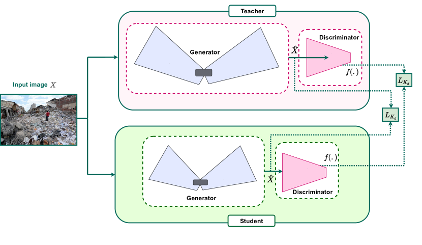
Figure 1: Overview of the proposed method

III-A Student-Teacher Architecture

The basic architecture of the student and teacher networks is similar, which helps in preventing information loss while tackling complex data [12]. The only difference is in the number of channels in each layers, where the student network has fewer channels in each layer than the teacher’s.

As Figure 2 illustrates (inspired by [27]), the student network architecture consists of a U-net [28] generator $G$ and a discriminator $D$ network. The generator has an encoder-decoder structure in which the encoder learns the discriminative feature representation of the training data by mapping the high dimensional input image $x$ into a low-dimension feature space $z$. The encoder’s role is to reconstruct the input image from the latent representation $z$. However, to have a more precise reconstructed image $\hat{x}$, the encoder layers are concatenated with their corresponding layers in the decoder network.

Interestingly, using the encoder-decoder structure alongside the skip-connections makes our student network robust in reconstructing complicated input images. These connections lead to a direct transfer of knowledge between layers while preserving local and global information. Besides the generator network, the discriminator architecture is an encoder adopted from the discriminator structure of DCGAN [29]. The goal of this network is to correctly distinguish real image $x$ from generated image $\hat{x}$ through the powerful network ${G}$. In addition, the discriminator obtains latent representations of the input image, regardless of whether it is classified as $x$ or $\hat{x}$.

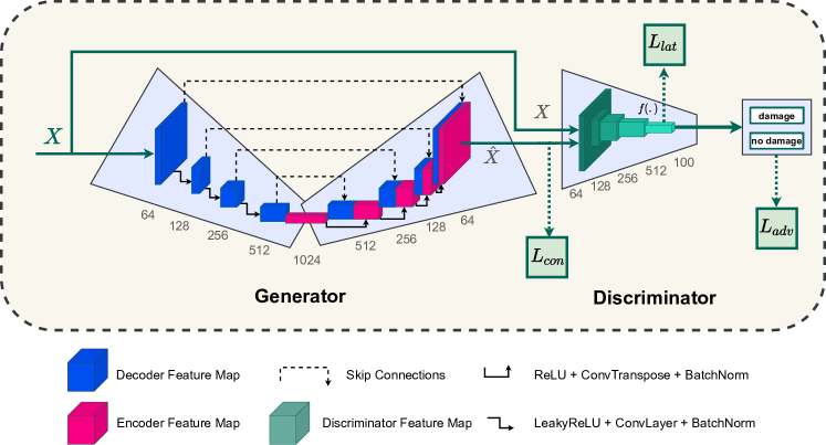
Figure 2: Details of the student network architecture.

III-B Training Student-Teacher

To apply KD framework, we extend the idea in [11] and employ intermediate feature representations of the teacher network to train the student network. In other words, the student network learns the full capability of the teacher model to generate training samples $\hat{x}$ and reconstruct latent representations for the input $x$ as close as possible. Motivated by [11], having a full knowledge transfer from teacher to student relies on considering the value and the direction of the activation functions’ values.

We assume that two activation vectors with similar Euclidean distances from a source vector do not necessarily have equal outputs in activating the following neuron. As a result, being in the same direction as well as the same Euclidean distance would result in more reliable knowledge transfer. For a selected critical layer $C_{m}$, we have:

$$L_{val}={\frac{1}{N_{i}}\sum_{j=1}^{N_{i}}{(a_{S}^{{C_{l}}_{i}}(j)-a_{T}^{{{C}_{l}}_{i}}(j))^{2}}}$$ (1)

$${L}_{dir}=1-\sum_{i}{\frac{vec(a_{S}^{{C_{l}}_{i}})^{T}.vec(a_{T}^{{C_{l}}_{i}})}{\left\lVert vec(a_{S}^{{C_{l}}_{i}})\right\rVert\;\left\lVert vec(a_{T}^{{C_{l}}_{i}})\right\rVert}}$$ (2)

where $N_{i}$ denotes the number of the neurons in layer ${C_{l}}_{i}$, $a_{.}^{{C_{l}}_{i}}(j)$ is the value of $j^{th}$ activation in layer ${C_{l}}_{i}$, and the $vec(x)$ indicates a vectorize function.

Therefore, to induce the student network to accurately emulate the teacher’s feature representations on input training samples, we select two critical layers as hints for transferring teacher knowledge. As depicted in Figure 1, the first one is the latent representations of discriminator ${D}$, which is defined here as ($f(.)$). The second one is the reconstructed image by generator $G$, which is defined as $\hat{x}$. For each critical layer $C_{m}$, $L_{val}$ tries to decrease the Euclidean distance, while $L_{dir}$ is used to increase the cosine similarity between the teacher and student output activation values. The KD losses, $K_{g}$ and $K_{d}$, are defined in Equation 3 and Equation 4, respectively.

$$L_{K_{g}}=L_{val}(\hat{x}_{S},\hat{x}_{T})+\alpha L_{dir}(\hat{x}_{S},\hat{x}_{T})$$ (3)

$$L_{K_{d}}=L_{val}(f_{S}(\hat{x}),f_{T}(\hat{x}))+\alpha L_{dir}(f_{S}(\hat{x}),f_{T}(\hat{x}))$$ (4)

where $\alpha$ is used to have the same range in the loss values. To choose the optimal value of $\alpha$, we consider the initial error amount before training for both terms [11].

Moreover, these critical layers are crucial for the student’s adversarial training. Inspired by [27], we use a combination of three losses ($L_{adv}$, $L_{con}$, $L_{lat}$) as the adversarial training objective. The Adversarial loss is the well-known MiniMax GAN loss, which helps the model generate realistic images. Contextual loss denotes the reconstruction error of the generated image $\hat{x}$. The Latent loss is defined to ensure that the network can contextually learn good latent representations of input data.

$$L_{adv}={\operatorname{\mathbb{E}}}_{x{\sim}p_{x}}{[logD(x)]}+{\operatorname{\mathbb{E}}}_{x{\sim}p_{x}}{[log(1-D(\hat{x})]}$$ (5)

$$L_{con}=\operatorname{\mathbb{E}}_{x\sim p_{x}}{\left\lVert x-\hat{x}\right\rVert_{1}}$$ (6)

$$L_{lat}=\operatorname{\mathbb{E}}_{x\sim p_{x}}{\left\lVert f(x)-f(\hat{x})\right\rVert_{2}}$$ (7)

Consequently, our training objective for the student network is defined as the weighted sum of all the above losses:

$$L=\lambda_{adv}L_{adv}+\lambda_{con}L_{con}+\lambda_{lat}L_{lat}+\lambda_{K_{g}}L_{K_{g}}+\lambda_{K_{d}}L_{K_{d}}$$ (8)

where $\lambda_{adv}$, $\lambda_{con}$ and $\lambda_{lat}$ are the parameters that specify the effectiveness of each loss in the total loss.

III-C Damage Detection

To detect damage, we pass the test samples to both the student and the teacher, which allows us to take advantage of the KD method. In particular, since the student network only learned manifold of the training data (no damage and has never seen such damaged images), it would represent different behavior on damage samples compared to the teacher, and it is likely to fail in reconstructing damages. Hence, the generator’s reconstructed image and the discriminator’s latent vector will help to distinguish damage data from no damage ones because the similarity of outputs between the student and teacher would decrease in these cases. For a given test sample $\dot{x}$, we formulate score $\mathcal{S}$ in Equation 9:

$$\mathcal{S}(\dot{x})=\omega_{L}\mathcal{L}(\dot{x})+\omega_{R}\mathcal{R}(\dot{x})+\omega_{VD}(\mathcal{V}(\dot{x})+\alpha\mathcal{D}(\dot{x}))$$ (9)

where $\mathcal{L}(\dot{x})$ calculates the similarity score between input image $x$ and the student’s generator reconstructed image $\hat{x}$ based on Equation 6, $\mathcal{R}(\dot{x})$ calculates the difference between the student’s discriminator latent representation of the input image $f(x)$ and the generated image $f(\hat{x})$ based on Equation 7, $\mathcal{V}(\dot{x})$ and $\mathcal{D}(\dot{x})$ measure similarity of teacher’s and student’s outputs in value and direction on the generated image, according to Equation 1 and Equation 2. $\omega_{L}$, $\omega_{R}$, and $\omega_{VD}$ adjust the effectiveness of the score functions in the final score, and $\alpha$ is defined as Equation 4 and Equation 3.

III-D Damage Localization

For the localization task, we investigate three gradient-based interpretability methods, namely: Vanilla Gradient [30], Smooth Gradient [31] and Guided Back-propagation [32]. These methods are based on the derivative of loss function w.r.t. the input to highlight the most important pixels. Figure 3 illustrates the results of these methods on damage test samples.

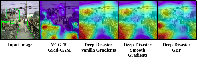
Figure 3: Different localization methods: First column: The input image, Second column: The localization of [9] method, Third-Fifth columns: Our localization results using three different localization methods.

III-D1 Vanilla Gradient

This method first computes a saliency map corresponding to the gradient of an output neuron with respect to the input, highlighting the areas of the given image [33]. We apply the Gradient method [30] on our final loss (Equation 8) to highlight the damaged areas in the test image samples. We are able to identify damages using this approach because these highlighted regions (i.e., damages) cause an increase in the gradient’s value. For a given input image $x$, the localization map is calculated as follows:

$${loc}_{map}(x)=\frac{\partial L}{\partial x}$$ (10)

where $L$ is the training objective function (Equation 8).

III-D2 Smooth Gradient

This method provides a less noisy saliency map by adding several input images perturbed with random Gaussian noise and averaging the resulting noisy gradients. This method extends any gradient-based interpretability method by adding a further step to the approach. We apply Smooth Gradient on the Vanilla Gradient Method to obtain a less noisy localization map. This approach is calculated as follows:

$${\hat{Loc}}_{map}(x)=\frac{1}{n}\sum_{1}^{n}{Loc}_{map}(x+\mathcal{N}(0,\,\sigma^{2}))$$ (11)

III-D3 Guided Back-propagation

This technique only uses the positive gradient with respect to input by back-propagating through the Relu activation function. As a result, we have only the positive gradients after changing the negative gradients’ values to zero, which means that the input features that activate the neurons would be highlighted.

IV Experimental Results

We evaluate the performance of Deep-Disaster on the Damage Assessment Dataset (DAD) [3] for detecting and localizing damages in different disaster types. Our model is implemented using PyTorch [34]. All reported results are performed using an NVIDIA GeForce RTX 2060 GPU.

The initial Learning rate of the student network is equal to $2e^{-3}$ with a decay rate. Also, momentum are equal to 0.5, with a batch size of 64. The hyper-parameters of our training objective function are: $\mathcal{\lambda}_{adv}=1$, $\mathcal{\lambda}_{lat}=1$, $\mathcal{\lambda}_{cons}=20$, $\mathcal{\lambda}_{K_{g}}=50$, and $\mathcal{\lambda}_{K_{d}}=1$. Moreover, we obtain optimum weights of Equation 9 by achieving the highest AUC-ROC using $\omega_{L}=0.4$, $\omega_{R}=0.2$, and $\omega_{VD}=0.4$.

IV-A Dataset

As the name implies, the DAD dataset is an imagery dataset to assess the level of damage in disaster events. The DAD contains social media images collected from AIDR [35]. The images from AIDR are gathered during four different natural disaster events: Philippines Ruby Typhoon (2014), Nepal Earthquake (2015), Ecuador Earthquake (2016), and USA Hurricane Matthew (2016). The dataset contains $\sim$25K images labeled into three classes of severity levels: severe, mild, and little-to-no damage.

However, following [8], we combine both the mild and severe classes into one class named damage, since we aim to train an unsupervised end-to-end network to distinguish no damage images from the damage ones. The original data splitting is: training (80%) and test (20%) [3]. Since we only used no-damage data during training, we followed the original dataset splitting for no-damage data (80%). Also, for evaluation, we kept the ratio (20%) for images data with no-damage and damage labels. Table I shows the class distribution for each disaster in the Train and Test phases.

TABLE I: DAD distribution on each disaster class for the train and test

Disaster name	Class labels	Train	Test
Ruby Typhoon	no damage	320	80
(486)	damage	-	86
Nepal Earthquake	no damage	6336	1584
(10156)	damage	-	2236
Ecuador Earthquake	no damage	730	182
(1186)	damage	-	274
Matthew Hurricane	no damage	261	65
(380)	damage	-	54

IV-B Evaluation Metric

The evaluation of our method is measured by the popular AUC-ROC metric. AUC-ROC measures performance for all possible classification thresholds calculating the area under the ROC curve. This metric assesses the capability of a model in distinguishing between classes. As a model approaches AUC-ROC of 1, the model’s accuracy improves. We utilize this metric to evaluate how our model performs in discriminating between no-damage and damage classes.

IV-C Ablation Studies

We conduct a series of ablation studies on the DAD dataset to answer the following questions: Is our Knowledge distillation structure really effective? Is student architecture improve the results (distillation effect)? Which layer/layers are effective while engaging in the training procedure?

IV-C1 Training Structure

For the first experiment, we compare four different architectures and training procedures: (1) Teacher network only, (2) Student network only, (3) Teacher and Student simultaneously from scratch, and (4) Student in the KD method using a pre-trained teacher. Figure 4 shows the AUC-ROC of all classes for these experiments. The results demonstrate that not only could we train a more compact network on the dataset, but also our framework outperforms all the other structures in this experiment.

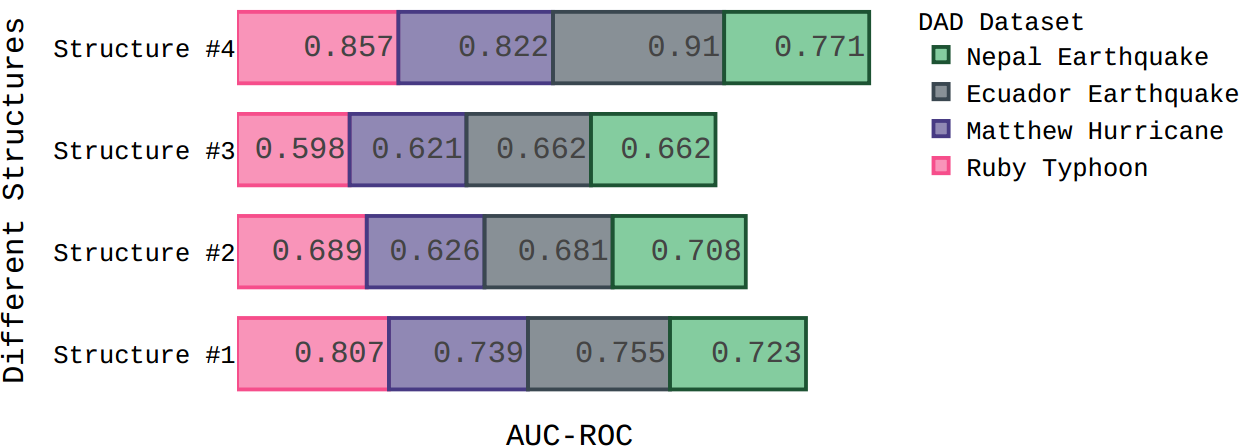
Figure 4: Comparison of AUC-ROC score on all classes for different training structures.

IV-C2 Distillation effect

For the next experiment, we investigate the effect of the student structure in our KD architecture. In the KD definition, a smaller student than the teacher helps to learn only distinguishing features and obliterating the non-distinguishing ones, especially in our unsupervised manner when there are only no damage data during training [11]. Table II shows that the smaller student achieves better performance than the equal size student for all classes, as we expected. The results originate from the fact that the images in the DAD dataset are hard to discriminate [14].

TABLE II: Comparison of AUC-ROC score on all classes for different student network size.

Ruby Typhoon Matthew Hurricane Ecuador Earthquake Nepal Earthquake Smaller 0.857 0.822 0.91 0.771 Equal 0.715 0.631 0.82 0.635

IV-C3 Intermediate Knowledge

To examine our KD method, we chose different layers for engaging in the training procedure; Figure 5 demonstrates that adding the $f(.)$ layer outperforms using solely the $\hat{x}$ layer; however, adding $z$ layer to the second training configuration does not enhance the results. The results confirm that increasing multiple features may not improve distilling knowledge. [12]

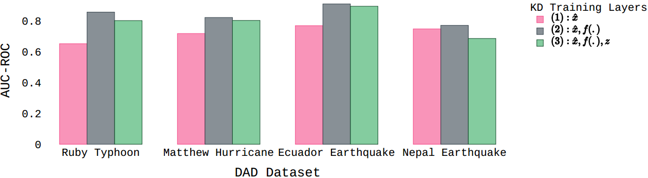
Figure 5: Comparing engaging different layers in the training procedure.

IV-D Results and Discussions

TABLE III: AUC-ROC results on the DAD dataset [3]

Category Method Ruby Typhoon Nepal Earthquake Ecuador Earthquake Matthew Hurricane Average Supervised VGG19 [19] 0.884 0.905 0.8846 0.765 0.85965 VGG19-unseen [19] 0.679 0.758 0.822 0.765 0.756 VGG16 [19] 0.897 0.898 0.9276 0.828 0.88765 VGG16-unseen [19] 0.655 0.795 0.817 0.768 0.75875 Domain Adaptation DANN [8] 0.732 0.738 0.795 0.779 0.761 DANN-unseen [7] 0.639 0.73 0.751 0.72 0.7105 SocialTrans [7] 0.742 0.779 0.839 0.806 0.7915 SocialTrans-unseen [7] 0.688 0.745 0.801 0.756 0.7475 Unsupervised Deep-Disaster 0.857 0.771 0.91 0.822 0.84 Deep-Disaster-unseen 0.765 0.803 0.945 0.701 0.8035

Table III presents a comparison between the performance of our proposed method and the state-of-the-art methods on the DAD dataset. As Table III shows, we achieved comparable results with the supervised methods and outperform domain adaptation methods. To the best of our knowledge, we are the first unsupervised approach for disaster detection trained on this dataset. Thus, to have a fair comparison, for each class, we report the average AUC-ROC score of testing on the rest of the classes’ trained models. The results marked by the ”unseen” label (i.e., SocialTrans-unseen) in the Table III illustrate that our method outperforms other methods in three out of four classes for novel disaster types and outperforms them on the overall average AUC-ROC score.

IV-D1 Localization

Our localization results in Figure 3 demonstrate that Deep-Disaster outperforms the model in [9], even though the latter is a supervised method. It shows that our model has learned the disasters and their discriminative features as well, despite the fact that we train it only on no damage images.However, we could not apply the Grad-CAM approach to our model as it is a supervised method requiring class-related localization weights. The results of the Vanilla Gradients and Smooth Gradients methods are visually similar, but the Smooth Gradients method exhibits less noisy localization since this method calculates an average over gradients of its noisy inputs. The GBP approach has competitive results compared to both methods, although it partially does image reconstructing and is unrelated to the network decision-making process [32].

IV-D2 Misclassified Images

To investigate images that our model does not recognize, we estimate a threshold on our damage detection score to find which images do not score appropriately [36]. As shown in Figure 6(a),(b), our model could not detect some images properly – most likely this due to lack of training data for some classes as they contain different kinds of no damage images (e.g., images containing text, or satellite images). Additionally, misclassification occurs because our training dataset (Tiny ImageNet) is not well enough to learn all the discriminative features during training the student network.

In addition, some images are not detected since they are very similar to the training samples or contain more than one scene. On the other hand, some images have not scored as images with damaged areas, even thought they were localized correctly (Figure 6(c),(d)). These discrepancies usually arise because there is no clear boundary between the definitions of class labels [14]. Consequently, in these such cases, the detection scores would not be distinguishable. Another consideration is the presence of identical images, especially in the Nepal Earthquake class, which affects the model’s performance drastically. These samples demonstrate the complexity of the DAD dataset.

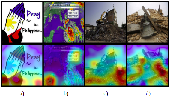
Figure 6: Samples of misclassified images. Each column contains the original image and its localization, respectively

V Conclusion

In this paper, we propose an efficient unsupervised method for disaster damage detection and localization based on visual data, which we call Deep-Disaster. Deep-Disaster is a KD method consisting of a pre-trained teacher and a smaller student network with similar architecture, where the intermediate knowledge of the teacher network is distilled on training images (no damage images) into the compact student network. Then, we detect the damaged areas using the networks’ different behavior in values and directions of their critical layers for the test images. In addition, we benefit from interpretability methods to extract localization maps. We used the DAD dataset to evaluate our method. The obtained results confirmed that our proposed method could detect damages without being explicitly trained on such damaged areas and gave an insight into the generalization capability of our method to novel disaster damages. A possible extension to this work is to conduct more experiments to determine the effectiveness of Deep-Disaster on the other mentioned disaster damage datasets and their various related tasks.

References

- [1]
- [2] F. Alam, F. Ofli, M. Imran, T. Alam, and U. Qazi, “Deep learning benchmarks and datasets for social media image classification for disaster response,” CoRR, vol. abs/2011.08916, 2020. [Online]. Available: https://arxiv.org/abs/2011.08916
- [3] D. T. Nguyen, F. Ofli, M. Imran, and P. Mitra, “Damage assessment from social media imagery data during disasters,” in 2017 IEEE/ACM International Conference on Advances in Social Networks Analysis and Mining (ASONAM), 2017, pp. 569–576.
- [4] F. Alam, F. Ofli, and M. Imran, “Crisismmd: Multimodal twitter datasets from natural disasters,” CoRR, vol. abs/1805.00713, 2018. [Online]. Available: http://arxiv.org/abs/1805.00713
- [5] H. Mouzannar, Y. Rizk, and M. Awad, “Damage identification in social media posts using multimodal deep learning.” in ISCRAM, 2018.
- [6] F. Alam, T. Alam, M. Hasan, A. Hasnat, M. Imran, F. Ofli et al., “Medic: A multi-task learning dataset for disaster image classification,” arXiv preprint arXiv:2108.12828, 2021.
- [7] Y. Zhang, R. Zong, and D. Wang, “A hybrid transfer learning approach to migratable disaster assessment in social media sensing,” 2020 IEEE/ACM International Conference on Advances in Social Networks Analysis and Mining (ASONAM), pp. 131–138, 2020.
- [8] X. Li, D. Caragea, C. Caragea, M. Imran, and F. Ofli, “Identifying disaster damage images using a domain adaptation approach,” in Proceedings of the 16th International Conference on Information Systems for Crisis Response And Management, 2019.
- [9] X. Li, H. Zhang, D. Caragea, and M. Imran, “Localizing and quantifying damage in social media images,” CoRR, vol. abs/1806.07378, 2018. [Online]. Available: http://arxiv.org/abs/1806.07378
- [10] X. Li, D. Caragea, X. Li, and M. Imran, “Localizing and quantifying infrastructure damage using class activation mapping approaches,” Social Network Analysis and Mining, vol. 9, pp. 1–15, 2019.
- [11] M. Salehi, N. Sadjadi, S. Baselizadeh, M. H. Rohban, and H. R. Rabiee, “Multiresolution knowledge distillation for anomaly detection,” CoRR, vol. abs/2011.11108, 2020. [Online]. Available: https://arxiv.org/abs/2011.11108
- [12] L. Wang and K.-J. Yoon, “Knowledge distillation and student-teacher learning for visual intelligence: A review and new outlooks,” IEEE Transactions on Pattern Analysis and Machine Intelligence, 2021.
- [13] F. Alam, M. Imran, and F. Ofli, “Image4act: Online social media image processing for disaster response,” 2017 IEEE/ACM International Conference on Advances in Social Networks Analysis and Mining (ASONAM), pp. 601–604, 2017.
- [14] D. T. Nguyen, F. Alam, F. Ofli, and M. Imran, “Automatic image filtering on social networks using deep learning and perceptual hashing during crises,” CoRR, vol. abs/1704.02602, 2017. [Online]. Available: http://arxiv.org/abs/1704.02602
- [15] K. R. Nia and G. Mori, “Building damage assessment using deep learning and ground-level image data,” in 2017 14th conference on computer and robot vision (CRV). IEEE, 2017, pp. 95–102.
- [16] H. Maeda, Y. Sekimoto, T. Seto, T. Kashiyama, and H. Omata, “Road damage detection using deep neural networks with images captured through a smartphone,” CoRR, vol. abs/1801.09454, 2018. [Online]. Available: http://arxiv.org/abs/1801.09454
- [17] F. Yuan and R. Liu, “Feasibility study of using crowdsourcing to identify critical affected areas for rapid damage assessment: Hurricane matthew case study,” International Journal of Disaster Risk Reduction, vol. 28, pp. 758–767, 2018. [Online]. Available: https://www.sciencedirect.com/science/article/pii/S221242091830150X
- [18] Y.-J. Cha, W. Choi, and O. Büyüköztürk, “Deep learning-based crack damage detection using convolutional neural networks,” Comput.-Aided Civ. Infrastruct. Eng., vol. 32, no. 5, p. 361–378, May 2017. [Online]. Available: https://doi.org/10.1111/mice.12263
- [19] K. Simonyan and A. Zisserman, “Very deep convolutional networks for large-scale image recognition,” arXiv preprint arXiv:1409.1556, 2014.
- [20] R. R. Selvaraju, A. Das, R. Vedantam, M. Cogswell, D. Parikh, and D. Batra, “Grad-cam: Why did you say that? visual explanations from deep networks via gradient-based localization,” CoRR, vol. abs/1610.02391, 2016. [Online]. Available: http://arxiv.org/abs/1610.02391
- [21] A. Chattopadhay, A. Sarkar, P. Howlader, and V. N. Balasubramanian, “Grad-cam++: Generalized gradient-based visual explanations for deep convolutional networks,” in 2018 IEEE Winter Conference on Applications of Computer Vision (WACV), 2018, pp. 839–847.
- [22] G. Hinton, O. Vinyals, and J. Dean, “Distilling the knowledge in a neural network,” arXiv preprint arXiv:1503.02531, 2015.
- [23] J. Gou, B. Yu, S. J. Maybank, and D. Tao, “Knowledge distillation: A survey,” International Journal of Computer Vision, vol. 129, no. 6, pp. 1789–1819, 2021.
- [24] P. Mishra, R. Verk, D. Fornasier, C. Piciarelli, and G. L. Foresti, “Vt-adl: A vision transformer network for image anomaly detection and localization,” arXiv preprint arXiv:2104.10036, 2021.
- [25] G. Wang, S. Han, E. Ding, and D. Huang, “Student-teacher feature pyramid matching for unsupervised anomaly detection,” arXiv preprint arXiv:2103.04257, 2021.
- [26] P. Bergmann, M. Fauser, D. Sattlegger, and C. Steger, “Uninformed students: Student-teacher anomaly detection with discriminative latent embeddings,” in Proceedings of the IEEE/CVF Conference on Computer Vision and Pattern Recognition, 2020, pp. 4183–4192.
- [27] S. Akçay, A. A. Abarghouei, and T. P. Breckon, “Skip-ganomaly: Skip connected and adversarially trained encoder-decoder anomaly detection,” CoRR, vol. abs/1901.08954, 2019. [Online]. Available: http://arxiv.org/abs/1901.08954
- [28] O. Ronneberger, P. Fischer, and T. Brox, “U-net: Convolutional networks for biomedical image segmentation,” CoRR, vol. abs/1505.04597, 2015. [Online]. Available: http://arxiv.org/abs/1505.04597
- [29] A. Radford, L. Metz, and S. Chintala, “Unsupervised representation learning with deep convolutional generative adversarial networks,” CoRR, vol. abs/1511.06434, 2016.
- [30] K. Simonyan, A. Vedaldi, and A. Zisserman, “Deep inside convolutional networks: Visualising image classification models and saliency maps,” arXiv preprint arXiv:1312.6034, 2013.
- [31] D. Smilkov, N. Thorat, B. Kim, F. B. Viégas, and M. Wattenberg, “Smoothgrad: removing noise by adding noise,” CoRR, vol. abs/1706.03825, 2017. [Online]. Available: http://arxiv.org/abs/1706.03825
- [32] J. T. Springenberg, A. Dosovitskiy, T. Brox, and M. Riedmiller, “Striving for simplicity: The all convolutional net,” arXiv preprint arXiv:1412.6806, 2014.
- [33] P. Linardatos, V. Papastefanopoulos, and S. Kotsiantis, “Explainable ai: A review of machine learning interpretability methods,” Entropy, vol. 23, no. 1, p. 18, 2021.
- [34] A. Paszke, S. Gross, F. Massa, A. Lerer, J. Bradbury, G. Chanan, T. Killeen, Z. Lin, N. Gimelshein, L. Antiga, A. Desmaison, A. Kopf, E. Yang, Z. DeVito, M. Raison, A. Tejani, S. Chilamkurthy, B. Steiner, L. Fang, J. Bai, and S. Chintala, “Pytorch: An imperative style, high-performance deep learning library,” in Advances in Neural Information Processing Systems 32, H. Wallach, H. Larochelle, A. Beygelzimer, F. d'Alché-Buc, E. Fox, and R. Garnett, Eds. Curran Associates, Inc., 2019, pp. 8024–8035. [Online]. Available: http://papers.neurips.cc/paper/9015-pytorch-an-imperative-style-high-performance-deep-learning-library.pdf
- [35] M. Imran, C. Castillo, J. Lucas, P. Meier, and S. Vieweg, “Aidr: Artificial intelligence for disaster response,” in Proceedings of the 23rd international conference on world wide web, 2014, pp. 159–162.
- [36] D. Fourure, M. U. Javaid, N. Posocco, and S. Tihon, “Anomaly detection: How to artificially increase your f1-score with a biased evaluation protocol,” CoRR, vol. abs/2106.16020, 2021. [Online]. Available: https://arxiv.org/abs/2106.16020