Study of finite volume number density fluctuation at RHIC energies in PNJL model for the search of QCD Critical Point

Abstract

The Quantum Chromo Dynamical (QCD) phase diagram can be explored in the heavy ion collision experiments. The non-monotonic behavior of the conserved number fluctuations are believed to be a signatures of the QCD phase transition and the Critical End Point (CEP) as a function of the collision energy. Due to the experimental limitations the elementary constituents produced, are evanescent, it is very difficult to measure the observables directly. So, we need theoretical approaches to estimate the values of different observables. The Polyakov-Nambu-Jona-Lasinio (PNJL) models of QCD is such an effective model, which posses the benefit of having characteristics similar to the observables. We present the number density fluctuation at RHIC energies and quantitative estimates of its contribution of critical fluctuations in PNJL model.

I Introduction

In order to study the early universe, we must have the knowledge of the matter, that existed at that time. Upon reproducing the matter with the exact density and temperature, existing at that time, in laboratory conditions, the characteristics of the early Universe can be studied. So far, the only possible way to do that is, to collide two heavy atomic nuclei, accelerated to energies of orders of a hundred GeV, inside a collider. The Relativistic Heavy Ion Collider (RHIC) at the Brookhaven National Library (BNL) and The Large Hadron Collider (LHC) at CERN are the two biggest colliders for this. Using the results of head-on collisions, it is possible to model the density and temperature that existed in the first instants of the formation of the Universe. Over the past few decades, physicists around the globe have been trying to recreate the matter, named quark-gluon plasma (QGP), by colliding together nuclei of atoms, with enough high energy, to produce trillion degree temperatures. At these high temperatures, matter stays in the QGP state for a fraction of a second.

When two particle beams collide head-on inside the tunnel of colliders, some of the matter changes state from hadronic state to QGP state. In this chiral phase transition, a first order phase transition may exist. The possible existence of a first order phase transition and the smooth cross-over implies that the transition line will end at a point. This point is known as the QCD critical point or critical end point (CEP) STAR ; STAR1 . The CEP at the end of first order line is a critical point where the phase transition is of second order. With respect to the phase diagram, the critical point is the point where the boundary between phases disappear. To obtain the critical point from a phase diagram, physicists observe the enhancement of fluctuations of final state observables, for example, the number of pions emitted in a collision or the ratio of the numbers of kaons and pions emitted, higher order moment of conserved quantity, multiplicity, etc..

The QGP matter formed in the heavy ion collision experiments has a finite volume which depends on the size of the colliding matter, center of mass energy and collision centrality. In the different centrality measurements of HBT radii, several efforts have been made to estimate the finite volume of the system adamova . These results suggest that the volume increases with centrality during the freeze out of the system. The effect of finite volume system has been studied in many theoretical models such as non-interacting bag model elze , chiral perturbation theory luscher ; gasser , Nambu–Jona-Lasinio (NJL) model nambu ; kiriyama , linear sigma model braun1 ; braun2 , Polyakov loop extended Nambu–Jona-Lasinio (PNJL) model fukushima ; ratti ; pisarski ; fukushima1 ; hansen ; ciminale ; ghosh ; deb1 ; abhijit ; bhattacharyya2010investigation ; deb2009mesonic and by the first principle study of pure gluon theory on space time lattices bazavov ; boyd ; engels ; fodor ; allton ; forcrand ; aoki ; megias . In the NJL model the finite size of a dense baryonic matter has been described by the induction of a charged pion condensation phenomenon. Recently in PNJL model, it has been observed that as the volume decreases, the critical temperature for the crossover transition decreases. For lower volumes, CEP is shifted to a domain with a higher chemical potential $\mu$ and lower temperature $T$ deb1 . All the theoretical results indicate that the location of CEP strongly depends on the size of the fireball of the heavy ion collision system.

In this present work, our aim is to find out the critical end point of the QCD phase diagram. To do so we will use an effective model - Polyakov-loop extended Nambu-Jona-Lasinio (PNJL) model. We will focus on the calculation of quark number density and will try to find the critical region from the quark number densities and compare the results with the experimental beam energy scan results tlusty2018rhic ; odyniec2019beam . In order to study the quark numbers at finite temperature and chemical potential, it is found that the quark-number density is determined by the corresponding dressed quark propagator only zong . The quark number densities are important thermodynamic quantities because the quark-number susceptibilities at finite temperatures and densities can be determined from the derivatives of the quark number density with respect to the chemical potential. Since the quark number susceptibilities are good signatures for predicting the critical end point, the quark number densities should also provide a good prediction for the location of CEP. Thus we can investigate the number densities in PNJL model in the search for QCD critical point.

In this paper, first, we discuss PNJL model for infinite and finite volume systems followed by the calculation of the quark number densities for light quarks and strange quarks for different beam energies of the infinite volume and finite volume system. From the nature of the quark number density, as a function of the center of mass energy, we will try to analyse the location of the critical point.

II PNJL Model

Effective models are very important in studying high energy physics. They are constructed with Lagrangians of simple mathematical structure having properties similar to that of QCD. PNJL model is such an effective model which gives good results at finite temperature and chemical potential. We shall consider the 2+1 flavor PNJL model with six quark interactions. In the PNJL model the gluon dynamics is described by the chiral point couplings between quarks (present in the NJL part) and a background gauge field representing Polyakov Loop dynamics. The Polyakov line is represented as,

$$L(\bar{x})={\cal P}{\rm exp}[i{\int_{0}}^{\beta}d\tau A_{4}{({\bar{x}},\tau)}]$$ (1)

where $A_{4}=iA_{0}$ is the temporal component of Eucledian gauge field $(\bar{A},A_{4})$, $\beta=\frac{1}{T}$, and $\cal P$ denotes path ordering. $L(\bar{x})$ transforms as a field with charge one under global Z(3) symmetry. The Polyakov loop is then given by $\Phi=(Tr_{c}L)/N_{c}$, and its conjugate by, ${\bar{\Phi}}=(Tr_{c}L^{\dagger})/N_{c}$.

The Lagrangian of the PNJL model with three flavours and $U_{A}(1)$ anomaly is given by :

$$\begin{split}\cal{L}&=\sum_{f=u,d,s}\overline{\psi}_{f}(i\gamma^{\mu}D_{\mu}-m_{f}+\gamma_{0}\mu)\psi_{f}+\frac{g_{S}}{2}\sum_{a=0}^{8}[(\overline{\psi}\lambda^{a}\psi)^{2}\\ &+(\overline{\psi}i\gamma_{5}\lambda^{a}\psi)^{2}]-g_{D}\{det[\overline{\psi}_{f}\frac{(1+\gamma_{5})}{2}\psi_{f^{\prime}}]+\\ &det[\overline{\psi}_{f}\frac{(1-\gamma_{5})}{2}\psi_{f^{\prime}}]\}-\mathcal{U^{\prime}}(\Phi[A],\overline{\Phi}[A];T)\end{split}$$ (2)

where, $D_{\mu}=\partial_{\mu}-iA_{\mu}$ and $A_{\mu}$ is the gauge field which absorbs the strong interaction coupling and is given by $A_{\mu}(x)=g_{S}A_{\alpha}^{\mu}\lambda^{\alpha}/2$. $f$ denotes the flavors $u$, $d$ or $s$ respectively. The matrices $P_{L,R}=(1\pm\gamma_{5})/2$ are respectively the left-handed and right-handed chiral projectors, and the other terms have their usual meaning, described in details in Refs. bhattacharyya2010investigation ; deb2009mesonic . The confinement/ deconfinement properties of the quarks are described by the effective potential $\mathcal{U}^{\prime}(\Phi,\bar{\Phi};T)$ (with the Vandermonde term $J[\Phi,\overline{\Phi}]=(27/24\pi^{2})[1-6\Phi\overline{\Phi}+4(\Phi^{3}+\overline{\Phi}^{3})-3(\Phi\overline{\Phi})^{2}]$) expressed as:

$$\frac{\mathcal{U}^{\prime}(\Phi[A],\overline{\Phi}[A];T)}{T^{4}}=\frac{\mathcal{U}(\Phi[A],\overline{\Phi}[A];T)}{T^{4}}-\kappa ln[J(\Phi,\overline{\Phi})]$$

where $\mathcal{U}(\phi)$ is a Landau-Ginzburg type potential given by,

$$\frac{\mathcal{U}(\Phi,\overline{\Phi};T)}{T^{4}}=-\frac{b_{2}(T)}{2}\overline{\Phi}\Phi-\frac{b_{3}}{6}(\Phi^{3}+\overline{\Phi}^{3})+\frac{b_{4}}{4}(\overline{\Phi}\Phi)^{2}$$ (3)

with $b_{2}(T)=a_{0}+a_{1}\left(\frac{T_{0}}{T}\right)+a_{2}\left(\frac{T_{0}}{T}\right)^{2}+a_{3}\left(\frac{T_{0}}{T}\right)^{3}$. For the effective potential, we can choose the following parameters : $T_{0}=0.19$ GeV, $a_{0}=6.75,a_{1}=-1.95,a_{2}=2.625,a_{3}=-7.44,b_{3}=0.75,b_{4}=7.5,\kappa=0.13$.

Now, we know that the energy of a quark can be written as, $E_{i}=\sqrt{p_{i}^{2}+m_{i}^{2}}$. Using this and Eq. (2), we can obtain the Grand potential density for the PNJL model in MFA (mean field approximation) as,

$$\begin{split}\Omega^{\prime}&=\mathcal{U}^{\prime}[\Phi,\overline{\Phi},T]+2g_{S}\sum_{f=u,d,s}\sigma_{f}^{2}-\frac{g_{D}}{2}\sigma_{u}\sigma_{d}\sigma_{s}-6\sum_{f}\int_{0}^{\Lambda}\frac{d^{3}p}{(2\pi)^{3}}E_{pf}\Theta(\Lambda-|\vec{p}|)\\ &-2\sum_{f}T\int_{0}^{\infty}\frac{d^{3}p}{(2\pi)^{3}}ln[1+3(\Phi+\overline{\Phi}e^{-(E_{pf}-\mu)/T})e^{-(E_{pf}-\mu)/T})+e^{-3(E_{pf}-\mu)/T})]\\ &-2\sum_{f}T\int_{0}^{\infty}\frac{d^{3}p}{(2\pi)^{3}}ln[1+3(\overline{\Phi}+{\Phi}e^{-(E_{pf}+\mu)/T})e^{-(E_{pf}+\mu)/T})+e^{-3(E_{pf}+\mu)/T})]\\ &=\Omega-\kappa T^{4}ln[J(\Phi,\overline{\Phi})]\end{split}$$ (4)

where, $\sigma_{f}^{2}=(\sigma_{u}^{2}+\sigma_{d}^{2}+\sigma_{s}^{2})$ ,$\sigma_{f}^{4}=(\sigma_{u}^{4}+\sigma_{d}^{4}+\sigma_{s}^{4})$ and $\Lambda$ is the three momentum cut off. The pressure of the strongly interacting matter can be written in terms of the potential density as,

$$P(T,\mu)=-\Omega(T,\mu)$$ (5)

and the number density of the quarks can be written as,

$$n_{q}(T,\mu)=-\frac{\partial{\Omega(T,\mu)}}{\partial{\mu}}$$ (6)

where T is the temperature and $\mu$ is the quark chemical potential. So far, we have discussed about PNJL model for infinite volume. Now we will discuss about its implementation in finite volume. To do this, the first step is to choose the proper boundary condition (Periodic for bosons but anti-periodic for fermions). This would give an infinite sum over the discrete momentum values, given by, $p_{i}=n_{i}\pi/R$ (where i=x,y,z and $n_{i}$ are all positive integers and R is the lateral size of a cubic volume). Then, the effects of surface and curvatures should be incorporated. However, in this calculations, we have taken up some simplifications, such as, (i) neglecting surface and curvature effects, (ii) treating the infinite sum as an integration over a continuous variation of momentum, (iii) not using any modification to the mean field parameters due to finite size effects, as was taken in deb1 .

III Results

In this present paper, we have discussed the location of critical point using PNJL model calculation considering both infinite volume and finite volume (with R=2 fm) system. Using PNJL model we have obtained data sets for the number density of quark in a system as a function of the temperature of the system at a fixed quark chemical potential ($\mu_{q}$) for different beam energies (7.7 , 11.5, 14.5, 19.6, 27, 39, 62.4, 130, 200 GeV). The quark number density ($n_{q}$) as a function of Temperature (T) and $n_{q}/T^{3}$ as a function of Temperature (T) are plotted. Using the PNJL model parameters we have also obtained similar datasets for strange and baryons number densities which are shown in a similar manner. The list of the value of constant $\mu$’s ($\mu_{S}$ is strange quark number density and $\mu_{B}$ is the number density of baryon) for different beam energies are shown in Table:1

Table 1: Value of $\mu_{q},\mu_{S}$, and $\mu_{B}$ for different beam energies

Beam Energy $(\sqrt{s}_{NN})$	7.7 GeV	11.5 GeV	14.5 GeV	19.6 GeV	27.0 GeV	39.0 GeV	62.4 GeV	130.0 GeV	200.0 GeV
$\mu_{q}$ (MeV)	140.33	105.33	88.00	68.67	52.00	37.33	24.33	12.00	8.00
$\mu_{S}$ (MeV)	127	117	112	106	101	97	94	90.14	90.34
$\mu_{B}$ (MeV)	421	316	264	206	156	112	73	36	24

In the graphs, we have highlighted the temperature points corresponding to the beam energy values used in BES. To get these temperature (T) and $T/\mu_{B}$ from the value of beam energies ($\sqrt{s_{NN}}$), we have used the following expressions, as was used by Cleymans cleymans2006comparison :

$$T(\mu_{B})=a-b\mu_{B}^{2}-c\mu_{B}^{4}$$ (7)

$$\mu_{B}(\sqrt{s})=\frac{d}{1+e\sqrt{s}}$$ (8)

where, $a=0.166\pm 0.002$GeV, $b=0.139\pm 0.016$ GeV^-1 , $c=0.053\pm 0.021$ GeV^-3 , and $d=1.308\pm 0.028$GeV, $e=0.273\pm 0.008$ GeV^-1 . The values of critical temperature, as obtained from calculations, is given in the following Table: 2

Table 2: Value of $T_{c}$ for different beam energies

Beam Energy $(\sqrt{s}_{NN})$	7.7 GeV	14.5 GeV	19.6 GeV	27.0 GeV	39.0 GeV	62.4 GeV	130.0 GeV	200.0 GeV
Light Quark (MeV)	228.70	233.50	234.65	235.50	235.95	236.20	236.25	236.25
Strange Quark (MeV)	234.20	234.55	234.70	234.75	234.75	234.90	234.95	234.95
Baryon (MeV)	153.15	211.75	219.40	226.50	231.25	234.15	235.65	235.90

III.1 Strange Quark

The strange quark number density ($n_{S}$) as a function of the Temperature (T) is shown in Figure. 1. The coloured lines in each case, corresponding to nine beam energy values (7.7 GeV, 11.5 GeV, 14.5 GeV, 19.6 GeV, 27.0 GeV, 39.0 GeV, 62.4 GeV, 130 GeV, 200 GeV). The $n_{S}$ vs.T graph have Poisson like nature, with its maxima at around T $\sim$ 160 MeV in case of infinite volume and around T $\sim$ 190 MeV for finite volume case.

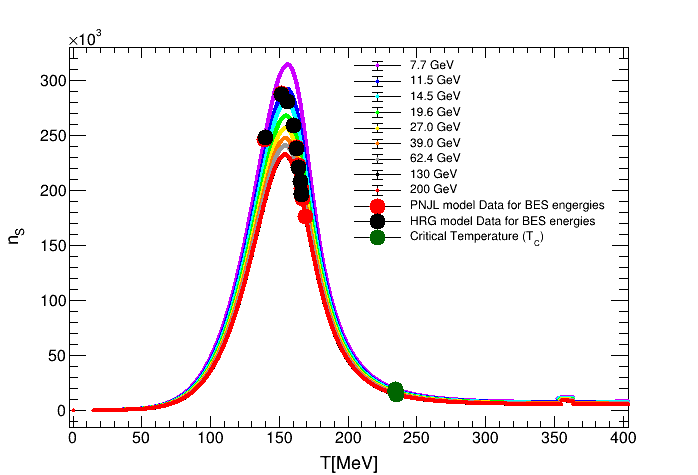
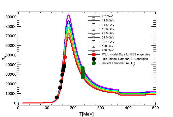
Figure 1: $n_{S}$ vs. $T$ plot for different beam energies. Left: infinite volume, right: finite volume with R=2 fm. Points corresponds to the temperature associated with BES energies from PNJL (red) and HRG (black) model.

Now, at the two sides of the maxima, the first order derivative or the slope of these curves (positive or negative) has maxima. The region between these two points is the critical region. So, we can expect that the critical end point lies near the maxima of these graphs. The green points refer to the values of critical temperature for each beam energy obtained from theoretical calculations. For each line, the green points are at the base of the Poisson curve. The red points corresponds to the beam energy points obtained using Eq. (7) and Eq. (8). The black points refer to similar calculation, correspond to the HRG model hrg_data . For the infinite volume case, both the red and black points lie near the maxima of the lines. But for the finite volume case, the points lie at far left from the maxima. PNJL and HRG model based calculations for BES energies are close to each other and the calculated $T_{c}$ values are close to 235 MeV for both the finite and infinite cases.

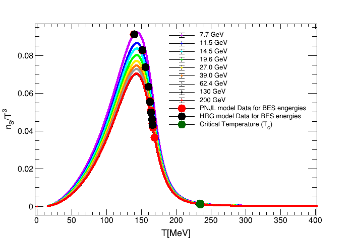
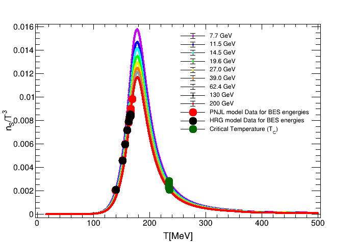
Figure 2: $n_{S}/T^{3}$ vs. $T$ for different beam energies. Left: infinite volume, right: finite volume with R=2 fm. Points corresponds to the temperature associated with BES energies from PNJL (red) and HRG (black) model.

The $n_{S}/T^{3}$ vs. T graphs in Figure. 2 have the same Poisson like nature. So, the nature of the slope of these curves, changes at the neighbourhood of the maxima. Therefore, we can expect that the critical point is present near the maxima of these curves too. In case of infinite volume, for lower beam energy (7.7 GeV, 11.5 GeV), the red and black points lie near the maxima of the lines. But, as the energy value increases, the points shift to the right of the maxima more and more. For finite volume case, these points are at the left of the maxima for each line (energy). The critical temperature points (green) lie near the base of the lines, for each case.

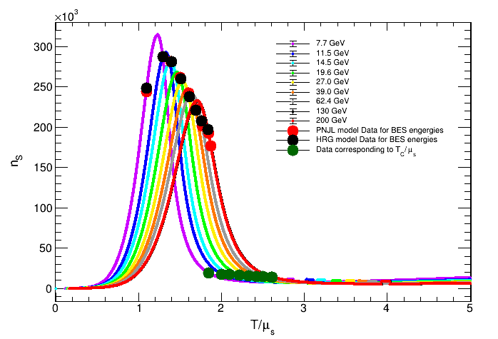
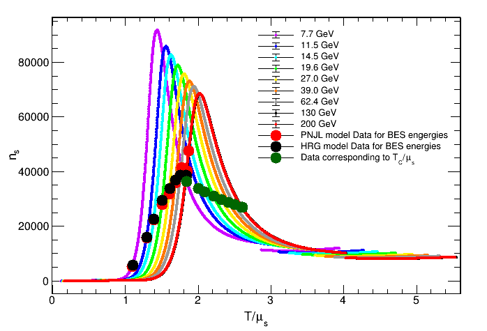
Figure 3: $n_{S}$ vs. $T/\mu_{q}$ plot for different beam energies. Left: infinite volume, right: finite volume with R=2 fm. Points corresponds to the temperature associated with BES energies from PNJL (red) and HRG (black) model.

The x-axis (temperature axis) of the $n_{S}$ vs. T graphs can be scaled by diving it by the value of constant $\mu_{S}$ for each beam energies to get $n_{S}$ vs. $T/\mu_{S}$ plots in Figure. 3. From the $n_{S}$ vs. $T/\mu_{S}$ plots, the peaks for different beam energies can be seen clearly. From these peaks, we can estimate the temperature at which, the critical end point may present. Red and black points lie near the maxima for lower beam energies in case of infinite volume, but far away from the peaks for finite volume system in all energies.

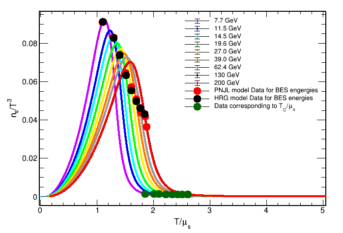
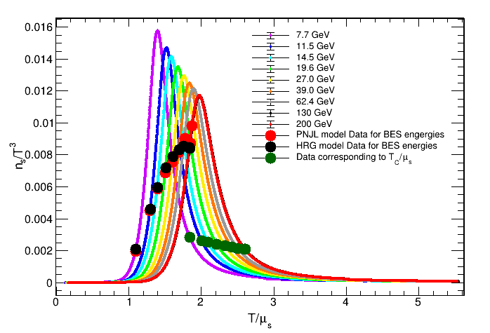
Figure 4: $n_{S}/T^{3}$ vs. $T/\mu_{q}$ plot for different beam energies. Left: infinite volume, right: finite volume with R=2 fm. Points corresponds to the temperature associated with BES energies from PNJL (red) and HRG (black) model.

The $n_{S}/T^{3}$ vs. $T/\mu_{S}$ plots in Figure. 4 have the same nature that of $n_{S}$ vs. $T/\mu_{S}$ plots. So, similar type of conclusions can be made from these graphs too. The position of the three types of points are similar to that of above plots.

III.2 Light Quark

The variations of $n_{q}/T^{3}$ as a function of $T$ for light quark for finite and infinite volume are shown in Figure. 5.

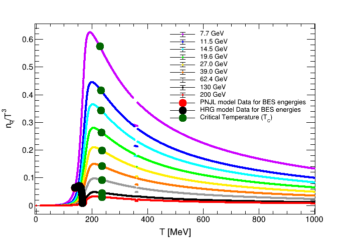
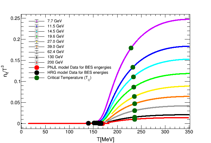
Figure 5: $n_{q}/T^{3}$ vs. $T$ plot for different beam energies. Left: infinite volume, right: finite volume with R=2 fm. Points corresponds to the temperature associated with BES energies from PNJL (red) and HRG (black) model.

This $n_{q}/T^{3}$ vs. T plots [5] do not have a Poisson like nature. These plots have a rapid change in their slope, in the small T region and the slope decreases slowly after the peak for the infinite volume case. An inflection point is located near to left of the peak, and another one is little bit further from the peak at right. So the critical point is assumed to be at the peak of the curves. The red and black points are very far away (at left) from the peak for every energy value. The $T_{C}$ points (green points) are located very near to the peak of the curves. In case of finite volume system size, the peaks are not present (may be due to unavailability of data). Both the calculated $T_{c}$ values are similar for finite and infinite cases.

The $n_{q}/T^{3}$ vs. $T/\mu_{q}$ plots in Figure. 6 have the same kind of nature as the $n_{q}/T^{3}$ vs. T graphs, as the only difference is that, the T axis is scaled by a factor of $\mu_{q}$ . So, the position of the CEP can also be estimated from these graphs. The calculated $T_{c}$ values (green points) are very near to the peak of the curves. Other two type of points (points corresponding to temperature associated with BES energies, calculated in PNJL and HRG model) are far away from the peak.

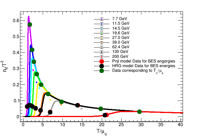
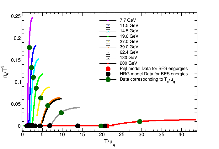
Figure 6: $n_{q}/T^{3}$ vs. $T/\mu_{q}$ plot for different beam energies. Left: infinite volume, right: finite volume with R=2 fm. Points corresponds to the temperature associated with BES energies from PNJL (red) and HRG (black) model.

The variations of $n_{q}$ as a function of $T$ for light quark for finite and infinite volume are shown in Figure. 7. The $n_{q}$ vs. T graphs have no maxima as such for both the finite and infinite volume. Finding CEP from this type of plot is difficult. In the region between the black and green points, there is an inflection point, where the slope of the curves have changed it’s nature. Critical point lies near to that point.

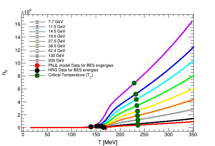
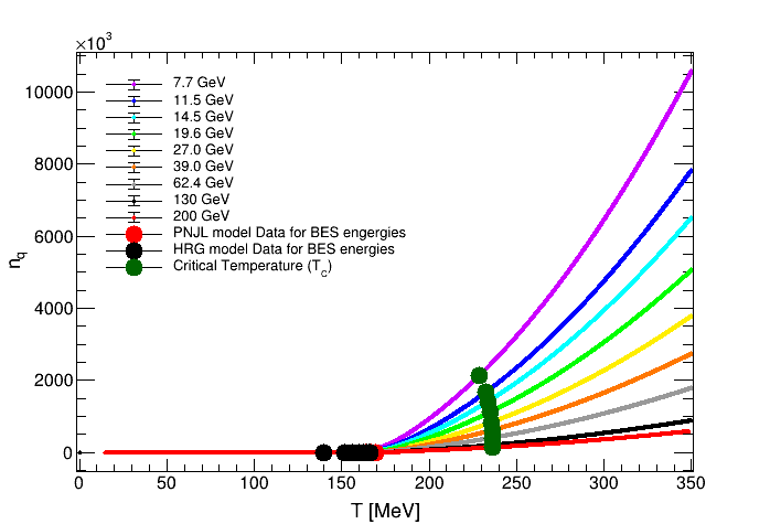
Figure 7: $n_{q}$ vs. $T$ plot for different beam energies. Left: infinite volume, right: finite volume with R=2 fm. Points corresponds to the temperature associated with BES energies from PNJL (red) and HRG (black) model.

Figure. 8 shows the variation of $n_{q}$ as a function of the temperature scaled with $\mu_{q}$ for finite and infinite volume. The $n_{q}$ vs. $T/\mu_{q}$ curves for different beam energies have a clear point of inflection for infinite volume case. For finite volume case, this point is not so clear. The green points lie at the right, and the black (and red) points lie at the left of that point. The HRG and PNJL calculations are in good agreement for all beam energies.

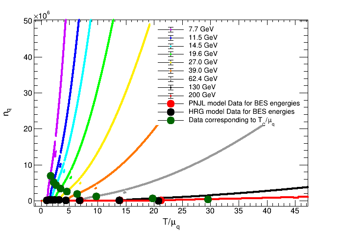
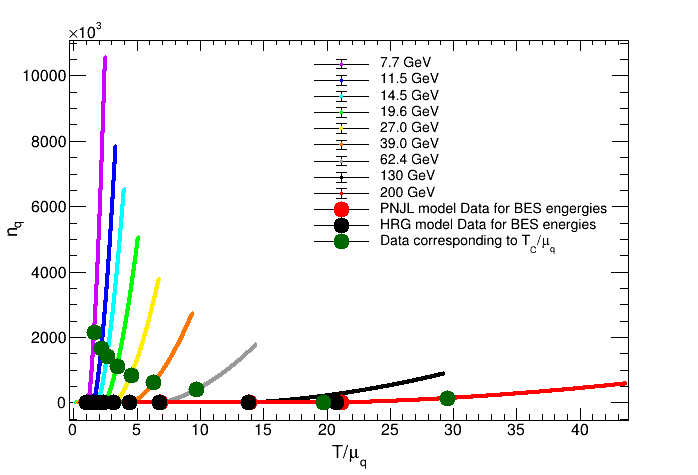
Figure 8: $n_{q}$ vs. $T/\mu_{q}$ plot for different beam energies. Left: infinite volume, right: finite volume with R=2 fm. Points corresponds to the temperature associated with BES energies from PNJL (red) and HRG (black) model.

III.3 Baryon

For baryon number density the variations of $n_{B}/T^{3}$ as a function of $T$ for infinite and finite volume are shown in Figure. 9 for different beam energies. The variations has similar dependency as in quark number density. These curves have a rapid change in their slope, in the small T region and the slope decreases slowly after the peak for the infinite volume case. A inflection point is located near to left of the peak, and another one is little bit further from the peak at right. So the critical point is assumed to be at the peak of the curves. The red and black points are very far away (at left) from the peak for every energy value. Calculation based on PNJL (red point) and on HRG model (black points) are also shown on the corresponding energy curves.

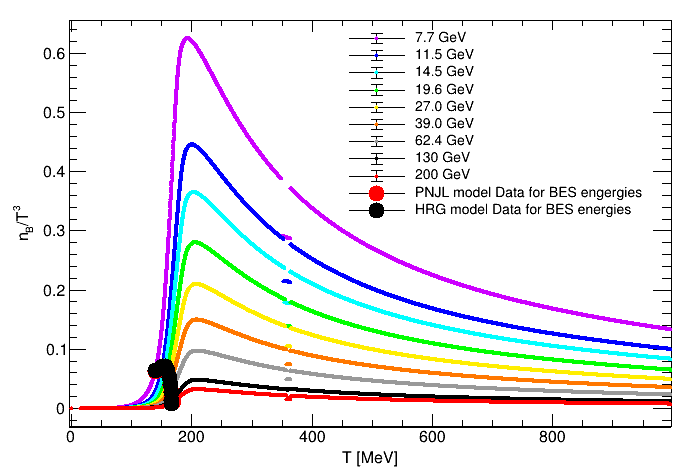
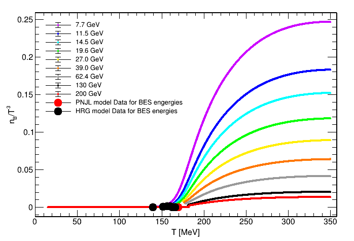
Figure 9: $n_{B}/T^{3}$ vs. $T$ plot for different beam energies. Left: infinite volume, right: finite volume with R=2 fm. Points corresponds to the temperature associated with BES energies from PNJL (red) and HRG (black) model.

Figure. 10 shows $n_{B}/T^{3}$ as a function of $T/\mu_{B}$ for different RHIC energies for infinite and finite volume. The position of the CEP can also be estimated from these graphs. The points corresponding to temperature associated with BES energies, calculated in PNJL and HRG model are also shown and are far away from the peak.

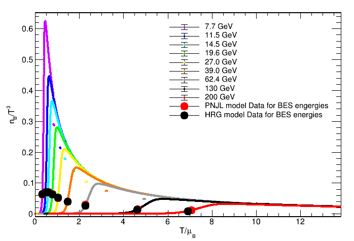
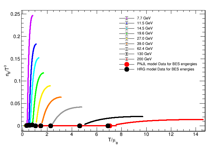
Figure 10: $n_{B}/T^{3}$ vs. $T/\mu_{B}$ plot for different beam energies. Left: infinite volume, right: finite volume with R=2 fm. Points corresponds to the temperature associated with BES energies from PNJL and HRG model.

The variations of $n_{B}$ as a function of $T$ for different energies for infinite and finite volume are shown in Figure. 11. Here also, the variations has similar dependency as in quark number density. These curves have no maxima as such for both the finite and infinite volume. Finding CEP from this type of plot is difficult.

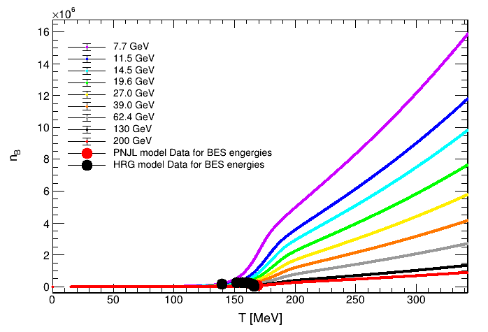
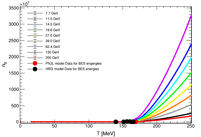
Figure 11: $n_{B}$ vs. $T$ plot for different beam energies. Left: infinite volume, right: finite volume with R=2 fm. Points corresponds to the temperature associated with BES energies from PNJL (red) and HRG (black) model.

The variations of $n_{B}$ as a function of $T/\mu_{B}$ for different energies for infinite and finite volume are shown in Figure. 12. The $n_{B}$ vs. $T/\mu_{B}$ curves for different beam energies have a clear point of inflection for infinite volume case. For finite volume case, this point is not so clear. The black (and red) points lie at the left of that point. The HRG and PNJL calculations are in good agreement for all beam energies. All of these four kinds of plots for the baryons show the exactly same nature as the quarks. So, the location of the critical points in the QCD phase diagram can be estimated from these plots similarly.

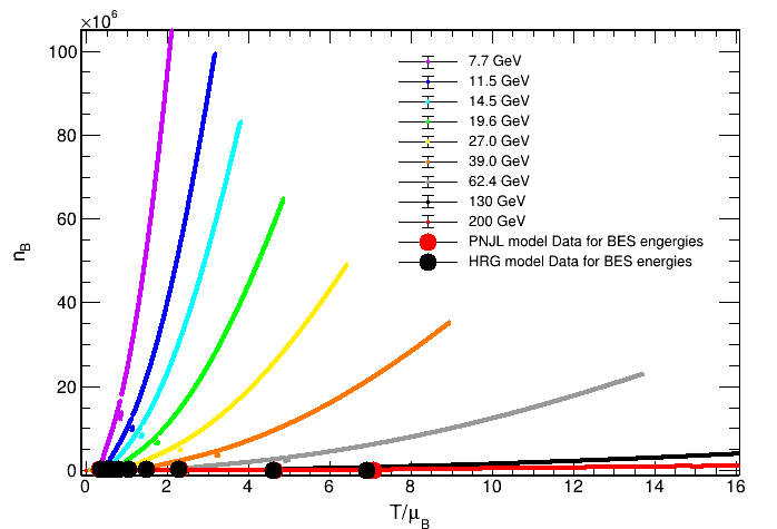
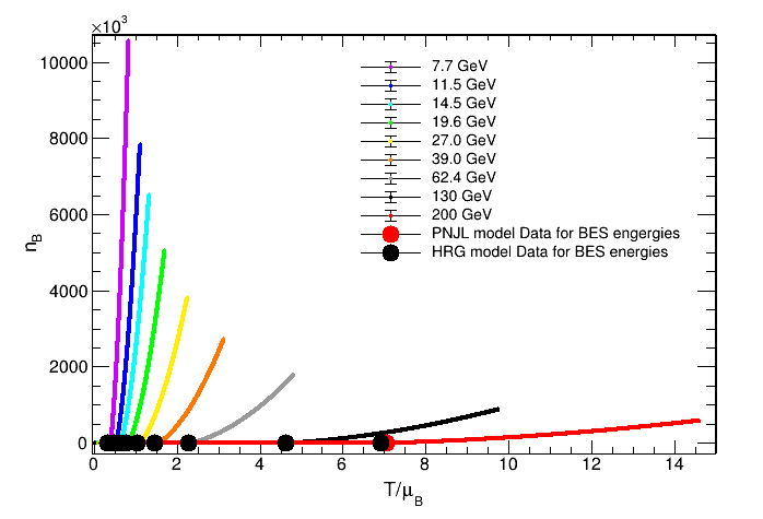
Figure 12: $n_{B}$ vs. $T/\mu_{B}$ plot for different beam energies. Left: infinite volume, right: finite volume with R=2 fm. Points corresponds to the temperature associated with BES energies from PNJL (red) and HRG (black) model.

IV Summary

In this work, we have tried to find out the critical end point of the QCD phase diagram in PNJL model. This is a very important work at hand, for high energy physicists, all over the world. This is so important because, by finding the CEP of the QCD phase diagram, we can get an idea about the critical point of the early universe, i.e, about the temperature and state of matter just after the Big Bang. To find the CEP, many different approaches are taken by different scientists at different times. With the advancement of technology in the world, we are not just stuck with the theoretical approaches. We have found paths to reach more close to the CEP in the experimental world. One of these aspects in the experimental world is the heavy ion collider. Inside these colliders, we can collide ions, protons, or so on, to get the elementary constituents of a particle. But as these collisions are instantaneous and the elementary constituents produced, are evanescent, it is very difficult to observe them directly. So, we need different models to estimate the values of different observables. The PNJL model is such an effective model. In our present study, we have discussed the formalism of the PNJL model briefly in section 2. In the following section, we have demonstrated our work to find the location of the critical end point. We have plotted the number density and number density/$T^{3}$ as a function of temperature and $T/\mu_{x}$ , where x stands for light quarks, strange quarks, and baryons. We have analyzed the nature of the curves and tried to find out the point of inflection (The point of inflection is the point on a curve, where a curve changes its nature.) and the maxima of the curves. The inflection point of the graph gives an estimation for the critical region and the maxima give an estimation for the CEP of the QCD phase diagram.

To conclude, we have studied the finite volume number density fluctuations at RHIC energies with system size both as finite and infinite in PNJL model. The variation of $n_{q}/T^{3}$ with T has the same nature in both these cases. The peak value for $n_{q}/T^{3}$ is around 0.44 for infinite volume and is around 0.18 in case of finite volume for $\mu$ =105.33 MeV (for $\sqrt{s}_{NN}$ =11.5 GeV) which is lesser than 0.44. For other beam energies this difference between peak values of $n_{q}/T^{3}$ can also be seen. The difference in peaks can also be seen in other kinds of plots too. So, we can conclude that the number density of the quarks and baryons are dependent on the size of the system. The nature of our $n_{S}$ vs. T (or $T/\mu_{q}$ ) and $n_{S}/T^{3}$ vs. T (or $T/\mu_{q}$ ) plots for strange quarks are like Poisson distributions. So, it has points of inflections at the two sides of the maxima. We have highlighted the temperature points corresponding to the BES energies on the curves. Some of these points, lie at the maxima, and some points lie at the two sides. These points lie in between the inflexion point and the maxima. Also, these points do not lie very near to the $T_{c}$ values. Therefore, the critical end point may not occur at the measured RHIC beam energy values exactly. So, at the energies, at which Beam Energy Scans are taken, we may not observe all the behaviors which occur at the critical point. Although, these measured points are located at the neighbourhood of the desired points, the measurement will have influence of critical region and the region near the critical end point can be explored by RHIC BES.

- (1) J. Adams et.al., Nucl. Phys. A 751 102–183 (2005).
- (2) M. M. Aggarwal et. al., Phys. Rev. C 82 024905 (2010).
- (3) D. Adamova et. al., Phys. Rev. Lett. 90, 022301 (2003).
- (4) H.-T. Elze and W. Greiner, Phys. Lett. B 179, 385 (1986).
- (5) M. Luscher, Commun. Math. Phys. 104, 177 (1986).
- (6) J. Gasser and H. Leutwyler, Phys. Lett. B 188, 477 (1987).
- (7) Y. Nambu and G. Jona-Lasinio, Phys. Rev. 122, 345 (1961); 124, 246 (1961).
- (8) O. Kiriyama and A. Hosaka, Phys. Rev. D 67, 085010 (2003).
- (9) J. Braun, B. Klein and P. Piasecki, Eur. Phys. Jr. C 71, 1576 (2011).
- (10) J. Braun, B. Klein and B.-J. Schefer, Phys. Lett. B 713, 216 (2012).
- (11) K. Fukushima, Phys. Lett. B 591 277 (2004).
- (12) C. Ratti, M.A. Thaler, and W. Weise, Phys. Rev. D 73 014019 (2006).
- (13) R.D. Pisarski, Phys. Rev. D 62 111501 (2000); A. Dumitru and R.D. Pisarski, Phys. Lett. B 504 282 (2001); 525 95 (2002); Phys. Rev. D 66 096003 (2002).
- (14) K. Fukushima, Phys. Rev. D 77 114028 (2008).
- (15) H. Hansen, W.M. Alberico, A. Beraudo, A. Molinari, M. Nardi, and C. Ratti, Phys. Rev. D 75 065004 (2007).
- (16) M. Ciminale, R. Gatto, N.D. Ippolito, G. Nardulli, and M. Ruggieri, Phys. Rev. D 77 054023 (2008).
- (17) S.K. Ghosh, T.K. Mukherjee, M.G. Mustafa, and R. Ray, Phys. Rev. D 73 114007 (2006); S.K. Ghosh, T.K. Mukherjee, M.G. Mustafa, and R. Ray, Phys. Rev. D 77 094024 (2008).
- (18) A. Bhattacharyya, P. Deb, S. K. Ghosh, R. Ray, S. Sur, Phys.Rev. D 87 054009 (2013).
- (19) A. Bhattacharyya, R. Ray and S. Sur, Phys. rev. D 91 051501 (2005).
- (20) A. Bhattacharyya, P. Deb, S. K.Ghosh, R. Ray, Phys. Rev. D 82 014021 (2010).
- (21) P. Deb, A. Bhattacharyya, S. Datta, and S.K. Ghosh,Phys. Rev. C 79 055208 (2009); A. Bhattacharyya, P. deb, A. Lahiri, R. Ray, Phys. Rev. D D 82 114028 (2010); A. Bhattacharyya, P. Deb, A. Lahiri, R. Ray, Phys. Rev. D 83 014011 (2011).
- (22) A. Bazavov and B. A. Berg, Phys. Rev. D 76, 014502 (2007).
- (23) G. Boyd et. al., Nucl. Phys. B 469 419 (1996).
- (24) J. Engels et. al., Nucl. Phys. B 558 307 (1999).
- (25) Z. Fodor and S.D. Katz, Phys. Lett. B 534 87 (2002); Z. Fodor, S.D. Katz, and K.K. Szabo, Phys. Lett. B 568 73 (2003).
- (26) C.R. Allton, S. Ejiri, S.J. Hands, O. Kaczmarek, F. Karsch, E. Laermann, Ch. Schmidt, and L. Scorzato, Phys. Rev. D 66 074507 (2002); C.R. Allton, S. Ejiri, S.J. Hands, O. Kaczmarek, F.Karsch, E. Laermann, and Ch. Schmidt, Phys. Rev. D 68 014507 (2003); C.R. Allton, M. Doring, S. Ejiri, S.J. Hands, O. Kaczmarek, F. Karsch, E. Laermann, and K. Redlich, Phys. Rev. D 71 054508 (2005).
- (27) P. de Forcrand and O. Philipsen, Nucl. Phys. B642 290 (2002); B673 170 (2003).
- (28) Y. Aoki, Z. Fodor, S.D. katz, and K.K. Szabo, Phys. Lett.B 643 46 (2006); Y. Aoki, G. Endrodi, Z. Fodor, S.D. Katz, and K.K.Szabo, Nature (London) 443 675 (2006).
- (29) E. Megias, E. Ruiz Arriola, and L.L. Salcedo, Rom. Rep.Phys.58, 081 (2006); E. Megias, E.R. Arriola, and L.L. Salcedo, Proc. Sci., JHW2005 (2006) 025; E. Megias, E.R. Arriola, and L.L. Salcedo, Nucl. Phys. B, Proc. Suppl.186 256 (2009); E. Megias, E.R. Arriola, and L.L. Salcedo, Phys. Rev. D 81, 096009 (2010).
- (30) D. Tlusty, arXiv:1810.04767.
- (31) G. Odyniec and STAR collaboration, PoS CORFU2018 151 (2019).
- (32) H-S. Zong and W-M. Sun, Phys. Rev. D 78 054001 (2008).
- (33) J. Cleymans, H. Oeschler, K. Redlich and S. Wheaton, Phys. Rev.C 73 034905 (2006).
- (34) F. Karsch and K. Redlich ,“Moments of charge fluctuations, pseudo-critical temperatures and freeze-out in heavy ion collisions ” Phys. Lett. B 695 (2011)