On a linearization of quadratic Wasserstein distance

Abstract.

This paper studies the problem of computing a linear approximation of quadratic Wasserstein distance $W_{2}$. In particular, we compute an approximation of the negative homogeneous weighted Sobolev norm whose connection to Wasserstein distance follows from a classic linearization of a general Monge-Ampére equation. Our contribution is threefold. First, we provide expository material on this classic linearization of Wasserstein distance including a quantitative error estimate. Second, we reduce the computational problem to solving a elliptic boundary value problem involving the Witten Laplacian, which is a Schrödinger operator of the form $H=-\Delta+V$, and describe an associated embedding. Third, for the case of probability distributions on the unit square $[0,1]^{2}$ represented by $n\times n$ arrays we present a fast code demonstrating our approach. Several numerical examples are presented.

1. Introduction

1.1. Introduction

Let $\mu$ and $\nu$ be probability measures supported on a bounded convex set $\Omega\subset\mathbb{R}^{N}$. The quadratic Wasserstein distance $W_{2}(\mu,\nu)$ is defined by

(1) $$W_{2}(\mu,\nu)^{2}:=\inf_{\pi}\int_{\Omega\times\Omega}|x-y|^{2}d\pi(x,y),$$

where the infimum is taken over all transference plans $\pi$ (probability measures on $\Omega\times\Omega$ such that $\pi[A\times\Omega]=\mu[A]$ and $\pi[\Omega\times A]=\nu[A]$ for all measurable sets $A$). Computing the quadratic Wasserstein distance is a nonlinear problem. In this paper, we consider the case where $\mu$ and $\nu$ have smooth positive densities $f$ and $g$ with respect to Lebesgue measure: $d\mu=fdx$ and $d\nu=g\,dx$. In this case, there is a classic local linearization of $W_{2}$ based on a weighted negative homogeneous Sobolev norm, which is derived from linearizing a general Monge–Ampére equation, see §2. In particular, the weighted negative homogeneous Sobolev norm $\|\cdot\|_{\dot{H}^{-1}(d\mu)}$ is defined for functions $u$ such that $\int_{\Omega}ud\mu=0$ by

(2) $$\|u\|_{\dot{H}^{-1}(d\mu)}:=\sup\left\{\int_{\Omega}u\,\varphi\,d\mu:\|\varphi\|_{\dot{H}^{1}(d\mu)}=1\right\},$$

where

(3) $$\|\varphi\|_{\dot{H}^{1}(d\mu)}^{2}:=\int_{\Omega}|\nabla\varphi|^{2}d\mu.$$

That is, the space $\dot{H}^{-1}(d\mu)$ is the dual space of $\dot{H}^{1}(d\mu)$. Under fairly general conditions, if $\delta\mu$ denotes a perturbation of $\mu$, then (informally speaking) we have

$$W_{2}(\mu,\mu+\delta\mu)=\|\delta\mu\|_{\dot{H}^{-1}(d\mu)}+o(\|\delta\mu\|),$$

see for example [Theorem 7.2.6 [29]] for a precise statement. Under stronger assumptions, if $\|\delta\mu\|=\varepsilon$, then the error term can be shown to be $\mathcal{O}(\varepsilon^{2})$, see §3.5 for details. In this paper, we study how to leverage the connection between the $\dot{H}^{-1}(d\mu)$-norm and the $W_{2}$ metric for computational purposes. In particular, our computational approach is based on a connection between the $\dot{H}^{-1}(d\mu)$-norm and the Witten Laplacian, which is a Schrödinger operator of the form

$$H=-\Delta+V,$$

where $V$ is a potential that depends on $f$, see Figure 1. We show that this connection provides a method of computation whose computational cost can be controlled by the amount of regularization used when defining the potential, see §4 for details.

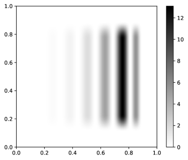
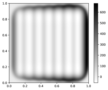
Figure 1. Function $f$ (left) and its regularized potential $V$ (right), see §5.4 for details about this example.

For the case of probability distributions on the unit square $[0,1]^{2}$ represented by $n\times n$ arrays, we present a code for computing this linearization of $W_{2}$ based on the Witten Laplacian, and present a number of numerical examples, see §5. This Witten Laplacian perspective leads to several potential applications; in particular, a method of defining an embedding discussed and methods of smoothing discussed in §6.

1.2. Background

The quadratic Wasserstein distance $W_{2}$ is an instance of Monge –Kantorovich optimal transport whose study was initiated by Monge [18] in 1781 and generalized by Kantorovich [12] in 1942. The theory of optimal transport has been developed by many authors; for a summary see the book by Villani [29]. Recently, due to new applications in data science and machine learning, developing methods to compute and approximate optimal transport distances has become an important area of research in applied mathematics, see the surveys by Peyré and Cuturi [22] and Santambrogio [25].

In this paper, we focus on the connection between the $W_{2}$ metric and the $\dot{H}^{-1}(d\mu)$-norm, which can be used to approximate $W_{2}$, see §2.3 and §3.5. The connection between $\dot{H}^{-1}(d\mu)$ and $W_{2}$ follows from the work of Brenier [3] in 1987 who discovered that under appropriate conditions the solution to Monge–Kantorovich optimal transport with a quadratic cost can be expressed using a map that pushes forward one measure to the other; moreover, this map is the gradient of a convex function, see §2.1. Brenier’s theorem reduces the problem of computing Wasserstein distance to solving a generalized Monge–Ampére equation. Linearizing this general Monge–Ampére equation gives rise to an elliptic equation, which corresponds to a weighted negative homogeneous Sobolev norm, see §2.3 below or see [§4.1.2, §7.6 of [29]]. The connection between Wasserstein distance and negative homogeneous Sobolev norms has been considered by several different authors as is discussed in the following section.

1.3. Related work

Several authors have considered the connection between negative homogeneous Sobolev norms and the $W_{2}$ metric in several different contexts. In analysis, this connection has been used to establish estimates by many authors, see for example [13, 15, 23, 26, 27]. Moreover, this connection also arises in the study of how measures change under heat diffusion, see [5, 21, 30]. The weighted negative homogeneous Sobolev norm has also been considered in connection to maximum mean discrepancy (MMD) which is a technique that can be used to compute a distance between point clouds, and has many applications in machine learning, see [1, 19, 20]. Authors have also considered this connection in papers focused on computing the $W_{2}$ metric, see [4, 9, 14]. Moreover, the negative homogeneous Sobolev norm has been considered in several applications to seismic image and image processing, see [8, 10, 31].

We emphasize three related works. First, Peyre [23] establishes estimates for the $W_{2}$ metric in terms of the unweighted negative homogeneous Sobolev norm $\|\cdot\|_{\dot{H}^{-1}(dx)}$. Let $\mu$ and $\nu$ be probability measures on $\Omega$ with densities $f$ and $g$ with respect to Lebesgue measure. The result of Peyre says that if $0<a<f,g<b<+\infty$, then

$$b^{-1/2}\|f-g\|_{\dot{H}^{-1}(dx)}\leq W_{2}(\mu,\nu)\leq a^{-1/2}\|f-g\|_{\dot{H}^{-1}(dx)};$$

a discussion and concise proof of this result can be found in [§5.5.2 of [25]]. Informally, this result says that if $\mu$ and $\nu$ have their mass spread out over $\Omega$, then the Wasserstein distance is equivalent to the negative unweighted homogeneous Sobolev norm of $f-g$; as a consequence, the weighted Sobolev norm is most interesting for probability distributions that have regions of high and low density.

Second, Engquist, Ren, and Yang [9] study the application of Wasserstein distance to inverse data matching. In particular, they compare the effectiveness of several different Sobolev norms for their applications; we note that the definitions of the norms they consider differ from the norm (2) that we consider, see the discussion in §3.6 below, but their results do indicate that negative homogeneous Sobolev norms may not be an appropriate substitute for the $W_{2}$ metric for some applications.

Third, Yang, Hu, and Lou [31] consider the implicit regularization effects of Sobolev norms in image processing. In §6 we mention a similar potential applications to image smoothing; our perspective is slightly different, but the underlying idea of this potential application is the same as [31].

2. Preliminaries and motivation

In this section, we briefly summarize material from Chapters 0.1, 0.2, 2.1, 2.3, 4.1, 4.2, and 7.6 of the book by Villani [29]. In order to make these preliminaries as concise as possible we state all definitions and theorems for our special case of interest; in particular, we assume that all probability measures have smooth densities with respect to Lebesgue measure, and restrict our attention to transport with respect to a quadratic cost function. This section is organized as follows: we consider the Monge-Kantorovich transport problem and Brenier’s theorem in §2.1, the Monge-Ampére equation in §2.2, and then discuss linearization of the $W_{2}$ metric in §2.3. The main purpose of these preliminaries is to provide background for (13), stated at the end of §2.3, which clarifies the statement that the $\dot{H}^{-1}(d\mu)$-norm is a linearization of the $W_{2}$ metric.

2.1. Monge-Kantorovich optimal transport and Brenier’s theorem

Let $\Omega\subset\mathbb{R}^{n}$ be a bounded convex set, and $\mu$ and $\nu$ be probability measures on $\Omega$ that have positive smooth densities $f$ and $g$, respectively, with respect to the Lebesgue measure. A transference plan $\pi$ is a probability measure on $\Omega\times\Omega$ such that

$$\pi[A\times\Omega]=\mu[A],\quad\text{and}\quad\pi[\Omega\times A]=\nu[A],$$

for all measurable subsets $A$ of $\Omega$. We denote the set of all transference plans by $\Pi(\mu,\nu)$, and define the transportation cost $I(\pi)$ with respect to the quadratic cost function $|x-y|^{2}$ by

$$I(\pi)=\int_{\Omega\times\Omega}|x-y|^{2}d\pi(x,y).$$

In this case, the Monge-Kantorovich optimal transport cost $\mathcal{T}(\mu,\nu)$ is defined by

(4) $$\mathcal{T}(\mu,\nu)=\inf_{\pi\in\Pi(\mu,\nu)}I(\pi).$$

Since we are considering a quadratic transportation cost, the Monge-Kantorovich optimal transport cost $\mathcal{T}(\mu,\nu)$ is the square of the $W_{2}$ metric:

(5) $$W_{2}(\mu,\nu)^{2}:=\mathcal{T}(\mu,\nu).$$

Under the above conditions, Brenier’s theorem states that the Monge-Kantorovich optimization problem (4) has a unique solution $\pi$ satisfying

(6) $$d\pi(x,y)=d\mu(x)\,\delta(y=\nabla\varphi(x)),$$

where $\varphi$ is a convex function such that $\nabla\varphi\#\mu=\nu$. Here $\#$ denotes the push-forward, and $\delta$ denotes a Dirac distribution. To be clear, given $T:\Omega\rightarrow\Omega$, the push-forward $\nu:=T_{\#}\mu$ is defined by the relation $\nu(A)=\mu(T^{-1}(A))$ for all measurable sets $A$, or equivalently, by the relation

$$\int_{\Omega}\zeta(x)d\nu(x)=\int_{\Omega}\zeta(T(x))d\mu(x),$$

for all continuous functions $\zeta$ on $\Omega$. Combining (4), (5), and (6) gives

(7) $$W_{2}(\mu,\nu)^{2}=\int_{\Omega}|x-\nabla\varphi(x)|^{2}d\mu(x).$$

2.2. Monge-Ampére equation

Recall that by assumption $\mu$ and $\nu$ have densities $f$ and $g$, respectively, with respect to the Lebesgue measure. We can express (6) as

$$\int_{\Omega}\zeta(\nabla\varphi(x))f(x)dx=\int_{\Omega}\zeta(y)g(y)dy,$$

for all bounded continuous functions $\zeta$ on $\Omega$. Changing variables $y=\nabla\varphi(x)$ on the right hand side and using the fact that $\zeta$ is arbitrary gives

(8) $$f(x)=g(\nabla\varphi(x))\det D^{2}\varphi(x).$$

Upon rearranging this equation as

$$\det D^{2}\varphi(x)=\frac{f(x)}{g(\nabla\varphi(x))},$$

it is clear that is an instance of the general Monge-Ampére equation

$$\det D^{2}\varphi(x)=F(x,\varphi,\nabla\varphi),$$

which has been studied by many authors, see for example [16, 17, 28].

2.3. Linearization of general Monge-Ampére equation

To linearize this general Monge-Ampére equation we assume that $f>0$ is positive, $\nabla\varphi\approx\operatorname{Id}$ is close to the identity, and $f\approx g$. More precisely, assume

(9) $$\varphi(x)=\frac{|x|^{2}}{2}+\varepsilon\psi(x),$$

and

(10) $$g(x)=\big{(}1+\varepsilon u(x)\big{)}f(x),$$

for some $\varepsilon>0$. Substituting (9) into (7) gives

(11) $$W_{2}(\mu,\nu)^{2}=\varepsilon^{2}\int_{\Omega}|\nabla\psi|^{2}d\mu,$$

which expresses $W_{2}(\mu,\nu)^{2}$ in terms of $\psi$. Substituting (9) and (10) into (8) gives

$$f=(1+\varepsilon u+\varepsilon^{2}R_{1})(f+\varepsilon\nabla f\cdot\nabla\psi+\varepsilon^{2}R_{2})(1+\varepsilon\Delta\psi+\varepsilon^{2}R_{3}),$$

where $R_{1},R_{2},R_{3}$ are remainder functions depending on $f,\psi$, $u$. It follows from rearranging terms that

(12) $$L\psi=u+\varepsilon R,$$

where

$$L\psi=-\Delta\psi-\nabla(\log f)\cdot\nabla\psi,$$

and $R$ denotes some remainder function depending on $f$, $\psi$, and $u$. Thus, if $\psi$ satisfies $L\psi=u$, then by (11) and (12) we expect that

(13) $$W_{2}(\mu,\nu)=\varepsilon\sqrt{\int_{\Omega}|\nabla\varphi|^{2}d\mu}+\mathcal{O}(\varepsilon^{2}),$$

which, roughly speaking, says that $L\psi=u$ is a linearization of the quadratic Wasserstein optimal transport problem, see §3.5 for a more precise version of (13).

3. Characterizing the operator $L$

So far we have presented background material that motivates why the quadratic Wasserstein distance $W_{2}$ is related to the operator $L$ defined by

$$L\psi=-\Delta\psi-\nabla(\log f)\cdot\nabla\psi.$$

In this section, we discuss the connection between the operator $L$, the negative weighted homogeneous Sobolev norm $\|\cdot\|_{\dot{H}^{-1}(d\mu)}$, and the quadratic Wasserstein distance $W_{2}$ in detail. The section is organized as follows: We start, in §3.1, by stating and proving a version of Green’s first identity that $L$ satisfies. Second, in §3.2 we state a result connecting the $\dot{H}^{-1}(d\mu)$-norm to the solution of an elliptic boundary value problem involving $L$. Third, in §3.3, we give a characterization of the $\dot{H}^{-1}(d\mu)$-norm in terms of a divergence optimization problem. Fourth, in §3.4 we consider a characterization of the $\dot{H}^{-1}(d\mu)$-norm involving the Witten Laplacian, which can be derived from $L$ by a change of variables. Fifth, in §3.5 we provide a more precise version of the statement that the $\dot{H}^{-1}(d\mu)$-norm is a linearization of the $W_{2}$ metric. Finally, in §3.6, we discuss weighted Sobolev norms in relation to the Fourier transform.

3.1. Green’s first identity analog for $L$

Let $\Omega$ be a bounded convex domain in $\mathbb{R}^{N}$, $\varphi$ be a once differentiable function, and $\psi$ be a twice differentiable function. Green’s first identity states that

(14) $$\int_{\Omega}\varphi(-\Delta\psi)dx=\int_{\Omega}(\nabla\varphi)\cdot(\nabla\psi)dx-\int_{\partial\Omega}\varphi(\partial_{n}\psi)ds,$$

where $\partial_{n}\psi=n\cdot\nabla\psi$, and $n$ is an exterior unit normal to the surface element $ds$.

Proposition 3.1.

Suppose that $\mu$ is a measure on $\Omega$ which has a density $f$ with respect to Lebesgue measure: $d\mu=fdx$. Further assume that $f$ is once differentiable, $f>0$ on $\Omega$, and $L:=-\Delta-\nabla(\log f)\cdot\nabla$. Then,

(15) $$\int_{\Omega}\varphi\,\,(L\psi)d\mu=\int_{\Omega}(\nabla\varphi)\cdot(\nabla\psi)d\mu,$$

whenever $\partial_{n}\psi=0$ on $\partial\Omega$ or $\varphi=0$ on $\partial\Omega$.

Proof.

By the definition of $L$ and the fact that $d\mu=fdx$ we have

$$\int_{\Omega}\varphi(L\psi)d\mu=\int_{\Omega}\varphi f(-\Delta\psi)-\varphi\,\,(\nabla f)\cdot(\nabla\psi)dx.$$

Since we assumed $\partial_{n}\psi$ or $\varphi$ vanishes on $\partial\Omega$ it follows from (14) that

$$\int_{\Omega}\varphi f(-\Delta\psi)-\varphi\,\,(\nabla f)\cdot(\nabla\psi)dx=\int_{\Omega}(\nabla(\varphi f))\cdot(\nabla\psi)-\varphi\,\,(\nabla f)\cdot(\nabla\psi)dx.$$

Finally, observe that expanding $\nabla(\varphi f)$ with the product rule and canceling terms gives:

$$\int_{\Omega}f\,\,(\nabla\varphi)\cdot(\nabla\psi)+\varphi(\nabla f)\cdot(\nabla\psi)-\varphi\,\,(\nabla f)\cdot(\nabla\psi)dx=\int_{\Omega}(\nabla\varphi)\cdot(\nabla\psi)d\mu,$$

which establishes (15). ∎

3.2. Elliptic boundary value problem

Let $\Omega$ be a bounded convex domain in $\mathbb{R}^{N}$, and suppose that $\mu$ is a measure on $\Omega$ which has a density $f$ with respect to Lebesgue measure: $d\mu=fdx$. Assume that $f$ is once differentiable and $f>0$ on $\Omega$. For functions $u$ such that $\int_{\Omega}ud\mu=0$ we define the $\dot{H}^{-1}(d\mu)$-norm by

$$\|u\|_{\dot{H}^{-1}(d\mu)}:=\sup\left\{\int_{\Omega}u\,\varphi\,d\mu:\|\varphi\|_{\dot{H}^{1}(d\mu)}=1\right\},$$

where

$$\|\varphi\|_{\dot{H}^{1}(d\mu)}^{2}:=\int_{\Omega}|\nabla\varphi|^{2}d\mu.$$

The following result characterizes the $\dot{H}^{-1}(d\mu)$-norm in terms of an elliptic boundary value problem involving the operator $L$.

Proposition 3.2.

We have

(16) $$\|u\|_{\dot{H}^{-1}}^{2}=\int_{\Omega}|\nabla\psi|^{2}d\mu=\int_{\Omega}\psi(L\psi)d\mu=\int_{\Omega}\psi\,u\,d\mu,$$

where $\psi$ is a solution to the elliptic boundary value problem

(17) $$\left\{\begin{array}[]{cc}L\psi=u&\text{in }\Omega\\ \partial_{n}\psi=0&\text{on }\partial\Omega,\end{array}\right.\quad\text{where}\quad L:=-\Delta+\nabla(-\log f)\cdot\nabla.$$

Proof of Proposition 3.2.

The second and third equalities in (16) are a direct consequence of the definition of $L$ and Proposition 3.1, so we only need to show that $\|u\|_{\dot{H}^{-1}}^{2}=\int_{\Omega}|\nabla\psi|^{2}d\mu$ . Assume that $\psi$ is a solution to (17) substituting $L\psi=u$. It follows from (15) that

(18) $$\int_{\Omega}u\,\varphi\,d\mu=\int_{\Omega}(L\psi)\,\varphi\,d\mu=\int_{\Omega}(\nabla\psi)\cdot(\nabla\varphi)\,d\mu.$$

Using the Cauchy-Schwarz inequality gives

$$\int_{\Omega}(\nabla\psi)\cdot(\nabla\varphi)d\mu\leq\left(\int_{\Omega}|\nabla\psi|^{2}d\mu\right)^{1/2}\left(\int_{\Omega}|\nabla\varphi|^{2}d\mu\right)^{1/2},$$

which implies that

$$\sup\left\{\int_{\Omega}u\,\varphi\,d\mu:\int_{\Omega}|\nabla\varphi|^{2}d\mu=1\right\}\leq\left(\int_{\Omega}|\nabla\psi|^{2}d\mu\right)^{1/2}.$$

On the other hand, from (18) we have

$$\int_{\Omega}u\,\varphi\,d\mu=\left(\int_{\Omega}|\nabla\psi|^{2}d\mu\right)^{1/2},\quad\text{when}\quad\varphi=\psi\left(\int_{\Omega}|\nabla\psi|^{2}d\mu\right)^{-1/2},$$

so we conclude that $\|u\|_{\dot{H}^{-1}}^{2}=\int_{\Omega}|\nabla\psi|^{2}d\mu$ as was to be shown. ∎

3.3. Divergence formulation

The $\dot{H}^{-1}(d\mu)$-norm can also be formulated as an optimization problem over vector fields satisfying a divergence condition. We note that our computational approach does not directly use this divergence formulation, and that our purpose of stating the following result is for completeness and its connection to other methods.

Proposition 3.3.

We have

$$\|u\|_{\dot{H}^{-1}(d\mu)}^{2}=\min_{F}\int_{\Omega}\|F\|^{2}d\mu,$$

where the minimum is taken over vector fields $F$ with continuous first-order partial derivatives that satisfy

(19) $$\left\{\begin{array}[]{cc}-\frac{1}{f}\operatorname{div}(fF)=u&\text{in }\Omega\\ n\cdot F=0&\text{on }\partial\Omega.\end{array}\right.$$

Note that it will become clear from the proof that it would suffice to assume that (19) holds in a weak sense.

Proof.

First, observe that if $\psi$ is a solution to the elliptic boundary value problem (17), then $F=\nabla\psi$ is admissible to the minimization since

$$-\frac{1}{f}\operatorname{div}(f\nabla\psi)=-\Delta\psi-\nabla(\log f)\cdot\nabla\psi=L\psi=u$$

and $n\cdot\nabla\psi=\partial_{n}\psi=0$. And from Proposition 3.2 we have

$$\|u\|_{\dot{H}^{-1}(d\mu)}^{2}=\int_{\Omega}|\nabla\psi|^{2}d\mu\geq\min_{F}\int_{\Omega}\|F\|^{2}d\mu.$$

To complete the proof it suffices to show that

$$\int_{\Omega}|\nabla\psi|^{2}d\mu\leq\min_{F}\int_{\Omega}\|F\|^{2}d\mu.$$

If we define $F=\nabla\psi+G$, then $G$ satisfies

$$\left\{\begin{array}[]{cc}-\frac{1}{f}\operatorname{div}(fG)=0&\text{in }\Omega\\ n\cdot G=0&\text{on }\partial\Omega.\end{array}\right.$$

Expanding $F=\nabla\psi+G$ gives

$$\int_{\Omega}\|F\|^{2}d\mu=\int_{\Omega}(|\nabla\psi|^{2}+2\nabla\psi\cdot G+|G|^{2})\,d\mu.$$

To complete the proof we will show that $\int_{\Omega}\nabla\psi\cdot G\,d\mu=0$. Observe that

$$\int_{\Omega}\nabla\psi\cdot G\,d\mu=-\int_{\Omega}\psi\frac{1}{f}\operatorname{div}(fG)\,d\mu+\int_{\Omega}\frac{1}{f}\operatorname{div}(\psi fG)\,d\mu.$$

The first integral on the right hand side is zero since $\frac{1}{f}\operatorname{div}(fG)=0$ in $\Omega$. The second integral on the right hand side is zero since by the Gauss divergence theorem

$$\int_{\Omega}\frac{1}{f}\operatorname{div}(\psi fG)d\mu=\int_{\Omega}\operatorname{div}(\psi fG)\,dx=\int_{\partial\Omega}\psi fG\cdot n\,ds,$$

and $n\cdot G=0$ by assumption. This completes the proof. ∎

3.4. Witten Laplacian formulation

The $\dot{H}^{-1}(d\mu)$-norm can also be defined in terms of a boundary value problem involving the Witten Laplacian $H$, which is a Schrödinger operator of the form

(20) $$H:=-\Delta+V,$$

where $V$ is a potential depending on $f$ defined by

$$V:=-\frac{1}{4}f^{-2}|\nabla f|^{2}+\frac{1}{2}f^{-1}\Delta f=f^{1/2}\Delta f^{-1/2}.$$

Alternatively, the Witten Laplacian $H$ can be defined by the similarity transform

(21) $$H\psi=f^{1/2}L(f^{-1/2}\psi),$$

which symmetrizes $L$ in the sense that the resulting operator $H$ is self-adjoint with respect to $L^{2}(dx)$; for a discussion of the Witten Laplacian and some spectral estimates see [6]. In the following Proposition, we give an elliptic equation involving $H$ that can be used to compute the $\dot{H}^{-1}(d\mu)$-norm; this proposition is an immediate consequence of the fact that the Schrödinger operator definition (20) is consistent with the similarity transform definition (21).

Proposition 3.4.

Using the notation $\tilde{u}=f^{1/2}u$ and $\tilde{\psi}=f^{1/2}\psi$ we have

$$\|u\|_{\dot{H}^{-1}(d\mu)}:=\left(\int_{\Omega}\tilde{u}(x)\tilde{\psi}(x)dx\right)^{1/2},$$

where $\tilde{\psi}$ is the solution to the elliptic boundary value problem:

$$\left\{\begin{array}[]{cc}H\tilde{\psi}=\tilde{u}&\text{in }\Omega\\ \tilde{\psi}=0&\text{on }\partial\Omega.\end{array}\right.$$

Proof.

This formulation is an immediate consequence of the identity

$$H\psi=f^{1/2}L(f^{-1/2}\psi)=-\Delta\psi+\left(-\frac{1}{4}f^{-2}|\nabla f|^{2}+\frac{1}{2}f^{-1}\Delta f\right)\psi,$$

which is straightforward to verify: expanding $f^{1/2}L(f^{-1/2}\psi)$ gives

$$H\psi=-f^{1/2}(\text{div}(f^{-1/2}(\nabla\psi)-\frac{1}{2}f^{-3/2}(\nabla f)\psi)-\frac{\nabla f}{f^{1/2}}\cdot(f^{-1/2}(\nabla\psi)-\frac{1}{2}f^{-3/2}(\nabla f)\psi),$$

$$=\frac{1}{2}f^{-1}(\nabla f)\cdot(\nabla\psi)-\Delta\psi+\frac{1}{2}f^{-1}(\nabla f)\cdot(\nabla\psi)-\frac{3}{4}f^{-2}\|\nabla f\|^{2}\psi+\frac{1}{2}f^{-1}(\Delta f)\psi\\ -f^{-1}(\nabla f)\cdot(\nabla\psi)+\frac{1}{2}f^{-2}|\nabla f|^{2}\psi),$$

and after canceling terms we have

$$H\psi=-\Delta\psi-\frac{1}{4}f^{-2}|\nabla f|^{2}\psi+\frac{1}{2}f^{-1}(\Delta f)\psi.$$

From the above calculation, it is also clear that

$$V=f^{1/2}\Delta f^{-1/2}$$

since all terms involving $\nabla f$ cancel. ∎

Remark 3.1 (Alternate form of the potential).

Using the fact that

$$\Delta(-\log f)=-f^{-1}\Delta f+f^{2}|\nabla f|^{2},$$

we can write $V$ as

$$V=\frac{1}{4}|\nabla F|^{2}-\frac{1}{2}\Delta F,$$

where $F:=-\log f$.

3.5. Linearization remainder estimate

Recall that previously in §2.3 we gave the informal estimate

$$W_{2}(\mu,\nu)=\varepsilon\sqrt{\int_{\Omega}|\nabla\Psi|^{2}d\mu}+\mathcal{O}(\varepsilon^{2}),$$

where $\Psi$ satisfies

$$L\Psi=u,\quad\text{where}\quad L:=-\Delta-\nabla(\log f)\cdot\nabla.$$

The purpose of this section, is to make this informal statement more precise; we emphasize that the result proved in this section is for illustrative purposes: results involving weaker assumptions and weaker regularity conditions are possible.

Let $\mu$ and $\nu$ be probability measures with densities $f$ and $g$ with respect to the Lebesgue measure: $d\mu=fdx$ and $d\nu=gdx$. Assume that

$$\varphi(x)=\frac{|x|^{2}}{2}+\varepsilon\psi(x),$$

where $\psi$ is a smooth function satisfying $\partial_{n}\psi=0$ on $\partial\Omega$. Further, assume that

$$g(x)=(1+\varepsilon u(x))f(x),$$

where $u$ is a smooth function. Assume that $\varphi$ satisfies the nonlinear equation

(22) $$f(x)=g(\nabla\varphi(x))\det D^{2}\varphi(x).$$

Let $\Psi$ be the solution to the elliptic boundary value problem

$$\left\{\begin{array}[]{cc}L\Psi=u&\text{in }\Omega\\ \partial_{n}\Psi=0&\text{on }\partial\Omega,\end{array}\right.\quad\text{where}\quad L:=-\Delta-\nabla(\log f)\cdot\nabla.$$

We have the following result.

Proposition 3.5.

Under the assumptions of §3.5 we have

$$|W_{2}(\mu,\nu)-\varepsilon\|u\|_{\dot{H}^{-1}(d\mu)}|\leq C_{\Omega,f,\psi,u}\varepsilon^{2},$$

where $C_{f,\psi,u}$ can be chosen in terms of almost everywhere upper bounds on:

$$|\nabla f|,|H_{f}|,|\nabla\psi|,|H_{\psi}|,|u|,|\nabla u|,|\Omega|,\text{ and }\lambda_{1}(L)^{-1},$$

where $|\nabla f|$ denotes the magnitude of the gradient of $f$, $|H_{f}|$ denotes the operator norm of the Hessian of $f$, $|\Omega|$ denotes the measure of $\Omega$, and $\lambda_{1}(L)$ denotes the smallest positive eigenvalue of $L$.

We demonstrate this result numerically in §5.3.

Proof of Proposition 3.5.

By the Lagrange remainder formulation of Taylor’s Theorem, and (22) we have

(23) $$f=(1+\varepsilon u+\varepsilon^{2}R_{1}))(f+\varepsilon\nabla f\cdot\nabla\psi+\varepsilon^{2}R_{2})(1+\varepsilon\Delta\psi+\varepsilon^{2}\det H_{\psi}),$$

where the remainder functions $R_{1},R_{2}$ can be expressed by

$$R_{1}(x)=\nabla u(\xi_{1})\cdot\nabla\psi(x),\quad\text{and}\quad R_{2}(x)=(\nabla\psi(x))^{\top}H_{f}(\xi_{2})\nabla\psi(x),$$

where $\xi_{1},\xi_{2}$ are points on the line segment between $x$ and $x+\varepsilon\nabla\psi(x)$. It follows that

(24) $$\varepsilon(-\Delta\psi-\nabla(\log f)\cdot\nabla\psi-u)f=\varepsilon^{2}R,$$

where the remainder function $\varepsilon^{2}R$ consists of all terms in the expansion of the right hand side of (23) that include $\varepsilon$ to power at least $2$. By the definition of $L$ and $\Psi$ we can rewrite (24) as

$$(L\psi-L\Psi)f=\varepsilon R.$$

Multiplying both sides of this equation by $\psi+\Psi$ and integrating over $\Omega$ gives

$$\int_{\Omega}(\psi+\Psi)(L\psi-L\Psi)d\mu=\varepsilon\int_{\Omega}(\psi+\Psi)R\,dx.$$

Using (15) to rewrite the left hand side gives

$$\int_{\Omega}|\nabla\psi|^{2}d\mu-\int_{\Omega}|\nabla\Psi|^{2}d\mu=\varepsilon\int_{\Omega}(\psi+\Psi)R\,dx.$$

By (9) and (16) it follows that

(25) $$W_{2}(\mu,\nu)^{2}-\varepsilon^{2}\|u\|_{\dot{H}^{-1}(d\mu)}^{2}=\varepsilon^{3}\left(\int_{\Omega}\psi Rdx+\int_{\Omega}\Psi Rdx\right).$$

We can bound the $L^{2}$ norm of $\Psi$ by the $L^{2}$ norm of $u$ and the inverse of the smallest positive eigenvalue of $L$; therefore, we can complete the proof by using Cauchy-Schwarz and almost everywhere bounds on all other quantities. ∎

Remark 3.2.

We note that it is possible to obtain various estimates on $|W_{2}(\mu,\nu)-\varepsilon\|u\|_{\dot{H}^{-1}(d\mu)}|$ from (25) in terms of $L^{p}$ norms of the quantities $\nabla f,H_{f},\nabla\varphi,H_{\psi},u,$ and $\nabla u$ instead of almost everywhere bounds. Moreover, results that guarantee bounds on the solution of general Monge-Ampére equations could be used to provide bounds for $\nabla\psi$ and $H_{\psi}$ in terms of $f$ and $u$, for example see [17].

3.6. Fourier transform and weighted Sobolev norms

In this section, we discuss a family of weighted Sobolev norms defined by Engquist, Ren, and Yang [9] using the Fourier transform

$$\hat{f}(\xi)=\int_{\mathbb{R}^{N}}f(x)e^{-2\pi ix\cdot\xi}dx.$$

In [9] the authors compare the $W_{2}$ metric to a family of weighted Sobolev norms defined in Fourier domain for the purpose of inverse data matching; in particular, in [Eq. 8 and Remark 2.1 of [9]] they define

(26) $$\|u\|_{\bar{H}^{s}(w)}^{2}=\int_{\mathbb{R}^{N}}\big{|}\widehat{w}*\widehat{u}_{s}\big{|}^{2}d\xi\quad\text{where}\quad\widehat{u}_{s}(\xi):=(2\pi|\xi|)^{s}\widehat{u}(\xi),$$

where $\widehat{w}$ and $\widehat{u}$ denote the Fourier transform of $w$ and $u$, respectively, and $*$ denotes convolution

$$(f*g)(x)=\int_{\mathbb{R}^{N}}f(x-y)g(y)dy.$$

Here we refer to the norm defined in (26) as the $\bar{H}^{s}(w)$-norm to avoid confusion with the $\dot{H}^{1}(d\mu)$-norm, which we defined in (3) by

$$\|\varphi\|_{\dot{H}^{1}(d\mu)}^{2}:=\int_{\Omega}|\nabla\varphi|^{2}d\mu,$$

and the $\dot{H}^{-1}(d\mu)$-norm defined in (2) by

$$\|u\|_{\dot{H}^{-1}(d\mu)}:=\sup\left\{\int_{\Omega}u\,\varphi\,d\mu:\|\varphi\|_{\dot{H}^{1}(d\mu)}=1\right\},$$

also see [§7.6 of [29]]. First, observe that if $s=1$ and $w=1$ is the constant function, then $\widehat{w}=\delta$ is the Dirac delta distribution and

$$\|u\|_{\bar{H}^{s}(w)}^{2}=\int_{\mathbb{R}^{N}}\big{|}(2\pi|\xi|)\widehat{u}(\xi)\big{|}^{2}d\xi=\int_{\mathbb{R}^{N}}\big{|}(2\pi i\xi)\widehat{u}(\xi)\big{|}^{2}d\xi=\int_{\mathbb{R}^{N}}|\nabla u|^{2}dx,$$

where the final inequality follows from the Plancherel theorem. However, if $s=1$ and $w$ is arbitrary, then in general

$$\|u\|_{\bar{H}^{s}(w)}^{2}=\int_{\mathbb{R}^{N}}|\widehat{w}*\widehat{u}_{1}|^{2}d\xi=\int_{\mathbb{R}^{N}}|u_{1}|^{2}w^{2}dx\not=\int_{\mathbb{R}^{N}}|\nabla u|^{2}w^{2}dx=\|u\|_{\dot{H}^{1}(d\mu)}^{2},$$

where $u_{1}$ denotes the inverse Fourier transform of $\widehat{u}_{1}(\xi)=2\pi|\xi|\widehat{u}(\xi)$, and $\mu$ is assumed to have density $w^{2}$ with respect to Lebesgue measure. It does follow from the Plancherel theorem that

$$\int_{\mathbb{R}^{N}}|u_{1}|^{2}dx=\int_{\mathbb{R}^{N}}|\nabla u|^{2}dx.$$

However, in general, the functions $|u_{1}|^{2}$ and $|\nabla u|^{2}$ are not equal, and thus in general their integrals against $w^{2}$ are not equal; in particular, their integrals against $w^{2}$ can be very different when $w^{2}$ is localized in space. Roughly speaking, the issue is that taking the absolute value of $\xi$ does not commute with taking the convolution. It is possible to define the $\dot{H}^{1}(d\mu)$-norm in Fourier domain by defining $\widehat{u}(\xi):=2\pi i\xi\widehat{u}$; however, this does not seem to lead to a viable way to compute the dual $\dot{H}^{-1}(d\mu)$-norm except in dimension $N=1$; we note that quadratic Wasserstein distance also has a simple characterization in $1$-dimension, see Remark 3.3.

Remark 3.3 ($W_{2}$ in $1$-dimension).

Let $\mu$ and $\nu$ be measures on $\mathbb{R}$ with densities $f$ and $g$ with respect to Lebesgue measure: $d\mu=fdx$ and $d\nu=g\,dx$. Let $F,G:\mathbb{R}\rightarrow[0,1]$ denote the cumulative distribution functions:

$$F(x)=\int_{-\infty}^{x}f(y)dy,\quad\text{and}\quad G(x)=\int_{-\infty}^{x}g(y)dy.$$

If $F^{-1}$ and $G^{-1}$ are the pseudo-inverse of $F$ and $G$ defined by

$$F^{-1}(t)=\min\{x\in\mathbb{R}:F(x)\geq t\}\quad\text{and}\quad G^{-1}(t)=\min\{x\in\mathbb{R}:G(x)\geq t\},$$

then

$$W_{2}(\mu,\nu)^{2}=\int_{0}^{1}(F^{-1}(t)-G^{-1}(t))^{2}dt,$$

see for example [Remark 2.30 of [22]].

4. Computation and regularization

In this section, we consider the connection between the $\dot{H}^{-1}(d\mu)$-norm and the Witten Laplacian, see §3.4, from a computational point of view. Recall that the Witten Laplacian is a Schrödinger operator of the form

$$H=-\Delta+V,$$

where $V$ is a potential. Roughly speaking, the advantage of considering this formulation is that all the complexity of the problem has been distilled into the potential $V$, which can be regularized to manage the computational cost. This section is organized as follows. First, in §4.1 we consider a spectral decomposition of $-\Delta$ by its Neumann eigenfunctions and define the fractional Laplacian $(-\Delta)^{\gamma}$. Second, in §4.2, we change variables using fractional Laplacians to precondition our elliptic equation involving $H$. Third, in §4.3, we observe how using the heat equation to define a smoothed version of $V$ can control the condition number of our problem. Finally, in §4.4 we discuss the computational cost of the described method.

4.1. Spectral decomposition of the Laplacian

Suppose that $\Omega$ is a bounded convex domain. Recall that $\lambda$ is a Neumann eigenvalue of the Laplacian $-\Delta$ on $\Omega$ if there is a corresponding eigenfunction $\varphi$ such that

$$\left\{\begin{array}[]{cc}-\Delta\varphi=\lambda\varphi&\text{in }\Omega\\ \partial_{n}\varphi=0&\text{on }\partial\Omega,\end{array}\right.$$

where $\partial\Omega$ denotes the boundary of $\Omega$, and $n$ denotes an exterior unit normal to the boundary. The Neumann eigenvalues of the Laplacian are nonnegative real numbers that satisfy

$$0=\lambda_{0}<\lambda_{1}\leq\lambda_{2}\leq\cdots\leq\lambda_{k}\leq\cdots\nearrow+\infty,$$

and the corresponding eigenfunctions $\{\varphi_{k}\}_{k=0}^{\infty}$ form an orthogonal basis of square integrable functions on $\Omega$. We can use this basis of Neumann eigenfunctions to define the fractional Laplacian $(-\Delta)^{\gamma}$ for $\gamma\in\mathbb{R}$ and $\psi=\sum_{k}\alpha_{k}\varphi_{k}$ by

$$(-\Delta)^{\gamma}\psi=\alpha_{0}\varphi_{0}+\sum_{k>0}\lambda_{k}^{\gamma}\alpha_{k}\varphi_{k},$$

where we include the constant term $\alpha_{0}\varphi_{0}$, independent of $\gamma$, so that the operator is well-defined and invertible for both positive and negative $\gamma$. With this definition, the operator $(-\Delta)^{\gamma}$ is invertible, which will become relevant in the following section; in particular, we will use the invertible operator $(-\Delta)^{\gamma}$ to precondition the elliptic equation $H\psi=u$.

4.2. Preconditioning the elliptic equation

Recall that our goal is to solve the elliptic equation

(27) $$H\psi=(-\Delta+V)\psi=u,$$

with Neumann boundary conditions; note that to simplify notation we dispense with the tilde notation $\tilde{\psi}$ and $\tilde{u}$ from §3.4 and just write $\psi$ and $u$. In order to precondition (27) we define $U$ and $\Psi$ by

$$U:=(-\Delta)^{1/2}u\quad\text{and}\quad\Psi:=(-\Delta)^{1/2}\psi.$$

It follows that

(28) $$A\Psi=U$$

where

$$A:=\operatorname{Id}-P_{1}+(-\Delta)^{-1/2}V(-\Delta)^{-1/2},$$

where $P_{1}$ denotes the projection onto the space of constant functions,

$$(P_{1}\Psi)(x)=\frac{1}{|\Omega|}\int_{\Omega}\Psi(y)dy,$$

and $\operatorname{Id}$ denotes the identity operator. We remark that the projection $P_{1}$ is necessary in the definition of $A$ since we have defined $(-\Delta)^{-1/2}$ to preserve constant functions, while the Laplacian $-\Delta$ destroys constant functions.

Since $(-\Delta)^{-1/2}$ is invertible the dimension of the null space of $A$ is the same as the dimension of the null space of $H$, which is $1$-dimensional. In particular, we have

$$Hf^{-1/2}=0,\quad\text{and}\quad A(-\Delta)^{1/2}f^{-1/2}=0.$$

Let $\lambda_{1}(H)$ and $\lambda_{1}(A)$ denote the smallest positive eigenvalue of $H$ and $A$, respectively. If $\psi_{1}(H)$ is a normalized eigenvector associated with $\lambda_{1}(H)$, then it follows from the Courant-Fisher Theorem that

$$\lambda_{1}(A)\geq c\lambda_{1}(H),$$

where $c=(\int_{\Omega}\|\nabla\psi_{1}(H)\|^{2}dx)^{-1}$. In the following, we treat $c$ as a fixed constant, which empirically we find is the case. Under this assumption, the condition number of $A$ on the space of functions orthogonal to $(-\Delta)^{1/2}f^{-1/2}$ is bounded by the operator norm of $A$, which satisfies

$$\|A\|^{2}\leq 1+\|V\|_{L^{\infty}},$$

If $f$ is an arbitrary smooth positive function, then $V$ could still take very large values, which could make our problem ill-conditioned. In the following section, we introduce a definition of $V$ that includes smoothing which can be used to control its $L^{\infty}$-norm.

4.3. Smoothing when defining the potential

Recall that the potential $V$ in the definition of $H$ can be defined by

$$V:=f^{-1/2}\Delta f^{1/2}.$$

The basic idea is to run the heat equation on $f^{1/2}$ and use the resulting smoothed function to define the potential $V$. Given a function $f$, we define a $1$-parameter family of norms parameterized by $\tau>0$ as follows. Let $\{\lambda_{k}\}_{k=0}^{\infty}$ and $\{\varphi_{k}\}_{k=0}^{\infty}$ denote the Neumann Laplacian eigenvalues and eigenfunctions, see §4.1. We define the Neumann heat kernel $e^{-\tau\Delta}$ for a function $\psi=\sum_{k}\alpha_{k}\varphi_{k}$ by

$$e^{-\Delta t}\psi=\sum_{k}e^{-\tau\lambda_{k}}\alpha_{k}\varphi_{k}.$$

Next, we define the smoothed potential $V_{\tau}$ by

(29) $$V=f^{-1/2}_{\tau}\Delta f^{1/2}_{\tau},\quad\text{where}\quad f_{\tau}:=(e^{-\tau\Delta}f^{1/2})^{2},$$

and define the corresponding operator $H_{\tau}$ by

$$H_{\tau}:=-\Delta+V_{\tau}.$$

By §3.4, the operator $H_{\tau}$ defines a $\dot{H}^{-1}(d\mu_{\tau})$-norm, where $\mu_{\tau}$ is the measure with density $f_{\tau}$. Observe that if $\tau=0$ then $\|u\|_{\dot{H}^{-1}(d\mu_{\tau})}=\|u\|_{\dot{H}^{-1}(d\mu)}$, while when $\tau\rightarrow\infty$ then $\|u\|_{\dot{H}^{-1}(d\mu_{\tau})}\rightarrow\|u\|_{\dot{H}^{-1}(dx)}$. In particular, we have

$$\|V_{\tau}\|_{L^{\infty}}\rightarrow 0,\quad\text{as}\quad\tau\rightarrow\infty,$$

so the parameter $\tau$ can be used to control the condition number of $H$, and hence can be used to control the computational cost as is discussed in the following section.

4.4. Computational cost

Computing the $\dot{H}^{-1}(d\mu_{\tau})$-norm using the operator

$$H_{\tau}=-\Delta+V,$$

involves solving an elliptic equation involving $H_{\tau}$. By §4.2 this equation can be preconditioned by a change of variables resulting in a linear system

$$A_{\tau}\Psi=U,$$

where $A_{\tau}$ is an operator with condition number $\mathcal{O}(\sqrt{1+\|V_{\tau}\|_{L^{\infty}}})$. Since $A_{\tau}$ is positive definite on the space orthogonal to its null space, and since $U$ is contained in this space, we can use Conjugate Gradient to solve this linear system to a fixed precision $\varepsilon>0$ with computational cost

$$C_{\text{solve}}=\mathcal{O}\left(C_{A}\sqrt{1+\|V_{\tau}\|_{L^{\infty}}}\right),$$

where $C_{A}$ is the cost to apply $A$. The operator $A$ can be applied quickly if we can efficiently change between the standard basis and the basis of Neumann Laplacian eigenfunctions. In the following remark, we discuss the case $\Omega=[0,1]^{2}$, where this transformation can be performed by a Discrete Cosine Transform (DCT).

Remark 4.1 (Spectral decomposition of Laplacian on unit square).

In the case $\Omega=[0,1]^{2}$, the Neumann Laplacian eigenvalues and eigenfunctions can be indexed by $k=(k_{1},k_{2})\in\mathbb{Z}_{>0}^{2}$ and are of the form

$$\lambda_{k}=k_{1}^{2}+k_{2}^{2}\quad\text{and}\quad\varphi_{k}(x)=c_{k_{1}}c_{k_{2}}\cos(\pi k_{1}x_{1})\cos(\pi k_{2}x_{2}),$$

where $x=(x_{1},x_{2})$ and $c_{k_{1}}$ and $c_{k_{2}}$ are constants to normalize $\varphi_{k}$ to have unit $L^{2}$ norm: $c_{k_{1}}=1/\sqrt{2}$ if $k_{1}>0$ and $c_{k_{1}}=1$ if $k_{1}=0$. Thus, expanding a function on the unit square in these Neumann eigenfunctions is equivalent to expanding a function in the double cosine series, which can be efficiently achieved by the Discrete Cosine Transform (DCT). In particular, if a function on the unit square $[0,1]^{2}$ is represented by an $n\times n$ array, then the computational cost of expanding in a double cosine series using the DCT is $\mathcal{O}(n^{2}\log n)$ operations.

5. Numerical examples

In this section we describe a numerical algorithm for using the Witten Laplacian to compute a local linear approximation of $W_{2}$ distance via the $\dot{H}^{-1}(d\mu_{\tau})$-norm. We use the analytical tools of the previous sections, and demonstrate the method on several numerical examples. In particular, this section is organized as follows: First, in §5.1 we describe the implementation of the algorithm and provide a link to code. In §5.2 we include analytical results about Wasserstein distance for Gaussian distributions and translations that we will use to interpret the numerical results. Third, in §5.3, we provide an initial numerical example for Gaussian distributions that illustrates the result of Proposition 3.5. Next, in §5.4 we provide illustrations of how the linearization approximates Wasserstein distance for translations. Fifth, in §5.5 we include visualizations of how the linearization approximates Wasserstein distance for changes in variance. Finally, in §5.7 we present an example of computing an embedding of the $\dot{H}^{-1}(d\mu)$-norm into $L^{2}$.

5.1. Implementation

Algorithm 5.1 (Linearized $W_{2}$ via Witten Laplacian).

We first compute the Witten potential, $V$, and then solve the resulting partial differential equation by converting it to a symmetric linear system which is solved using conjugate gradient.

1. Compute the potential $V_{\tau}$ using the smoothing procedure of section 4.3.

2. Solve the linear system

   $$A\Psi=U$$

   using conjugate gradient where $A$ is defined by (28).

   1. The discretized operator $A$ of (28) can be applied to a function, $f$, tabulated on an equispaced grid by first approximating $f$ as a $2$-dimensional cosine expansion of the form

      $$f(x_{1},x_{2})\approx\sum_{k_{1},k_{2}=0}^{n-1}\alpha_{k_{1},k_{2}}\cos(\pi k_{1}x_{1})\cos(\pi k_{2}x_{2})$$

      where $n$ is the number of function tabulations in each spatial dimension. The coefficients $\alpha_{k_{1},k_{2}}$ are computed with a Discrete Cosine Transform (DCT), which requires $O(n^{2}\log{n})$ operations.

   2. The operator $\Delta^{-1/2}$ of $A$ is applied to a cosine expansion via pointwise multiplication of the coefficients. For example, $\Delta^{-1/2}\cos(mx_{1})=-\frac{1}{m}\cos(mx_{1})$.

   3. Pointwise multiplication by $V_{\tau}$ in spatial domain is then performed with an inverse DCT, followed by pointwise multiplication in the spatial domain.

   4. Conjugate gradient is iterated until convergence up to some desired error tolerance.

We implemented the preceding algorithm in Python, and have provided publicly available codes with the implementation accessible at https://github.com/nmarshallf/witten_lw2.

5.2. Analytic formulas for $W_{2}$ for Gaussian distributions and translations

Let $\mu$ and $\nu$ be measures on $\mathbb{R}^{N}$ with densities $f$ and $g$ with respect to Lebesgue measure: $d\mu=fdx$ and $d\nu=gdx$. Assume that $f$ is a Gaussian function with mean $m_{f}$ and diagonal covariance $\Sigma_{f}=\operatorname{diag}(\sigma_{f}^{2})$, where $\sigma_{f}^{2}=(\sigma_{f,1}^{2},\ldots,\sigma_{f,N}^{2})$

$$f(x)=\frac{1}{(2\pi)^{d/2}(\det\Sigma_{f})^{1/2}}\exp\left(-\frac{1}{2}(x-m_{1})^{\top}\Sigma_{f}^{-1}(x-m_{f})\right).$$

Similarly, assume that $g$ is a Gaussian function with mean $m_{g}$ and covariance $\Sigma_{g}=\operatorname{diag}(\sigma_{g}^{2})$. Then,

(30) $$W_{2}(\mu,\nu)^{2}=|m_{f}-m_{g}|_{2}^{2}+|\sigma_{f}-\sigma_{g}|_{2}^{2}.$$

That is, the square of the quadradic Wasserstein distance between Gaussian distributions with diagonal covariance matrices is equal to the square of the distance between their means plus the square of the distance between their standard deviations, see [Remark 2.31 of [22]] for a more general result.

The dependence of quadratic Wasserstein distance on the distance between means for Gaussian distributions is a special case of a general translation property. Let $\mu$ and $\nu$ be two measures on $\mathbb{R}^{N}$ that have the same mean

$$\int_{\mathbb{R}^{N}}xd\nu=\int_{\mathbb{R}^{N}}xd\mu.$$

Let $T^{v}:\mathbb{R}^{N}\rightarrow\mathbb{R}^{N}$ denote the translation operator $T^{v}:x\mapsto x+v$. Suppose that $\nu_{v}$ denote a translation of $\nu$ by $v$; more formally, $\nu_{v}:=T^{v}_{\#}\nu$ where $\#$ denotes the push forward. Then quadratic Wasserstein distance satisfies the following relation:

(31) $$W_{2}(\mu,\nu_{v})^{2}=W_{2}(\mu,\nu)^{2}+|v|_{2}^{2},$$

That is, if two measures have the same mean and one measure is translated distance $|v|$, then the square of the quadratic Wasserstein distance between the measures increases by $|v|^{2}$, see [Remark 2.19 of [22]] for a slightly more general statement of this translation result.

5.3. Numerical example: linearization of $W_{2}$ for Gaussian distributions

In this section, we demonstrate that our code satisfies the result of Proposition 3.5 using Gaussian distributions and (30). Let $\mu$ and $\nu$ be measures on $\mathbb{R}^{N}$ with densities $f$ and $g$ with respect to Lebesgue measure: $d\mu=fdx$ and $d\nu=gdx$. We define $f:[0,1]^{2}\rightarrow\mathbb{R}$ by

(32) $$f(x)=\frac{1}{2\pi(\det\Sigma_{f})^{1/2}}\exp\left(-\frac{1}{2}(x-\mu_{f})^{\top}\Sigma_{f}^{-1}(x-\mu_{f})\right),$$

with

$$\mu_{f}=(1/2,\,\,1/2)^{\top}\qquad\text{and}\qquad\Sigma_{f}=\begin{pmatrix}1/16&0\\ 0&1/14\end{pmatrix},$$

and $g:[0,1]^{2}\rightarrow\mathbb{R}$ by

$$g(x)=\frac{1}{2\pi(\det\Sigma_{g})^{1/2}}\exp\left(-\frac{1}{2}(x-\mu_{g})^{\top}\Sigma_{g}^{-1}(x-\mu_{g})\right),$$

with

$$\mu_{g}=\mu_{f}+(0.001,\,\,0.002)^{\top}\qquad\text{and}\qquad\Sigma_{g}=\Sigma_{f}+\begin{pmatrix}0.001&0\\ 0&0.003\end{pmatrix}.$$

The covariances $\Sigma_{f}$ and $\Sigma_{g}$ are chosen such that, for numerical purposes up to precision $10^{-16}$, the functions $f$ and $g$, are essentially supported on $[0,1]^{2}$ and thus both are probability densities that integrate to $1$. For this numerical example, we use the above Python implementation of Algorithm 5.1 for the functions $f$ and $g$ tabulated on a $513\times 513$ equispaced grid on $[0,1]^{2}$, we define $u=(f-g)/f$, see §4.3. Recall that Proposition 3.5 says that if $\|u\|_{\dot{H}^{-1}(d\mu)}=\varepsilon$, then

$$|W_{2}(\mu,\nu)-\|u\|_{\dot{H}^{-1}(d\mu)}|=\mathcal{O}(\varepsilon^{2}).$$

The implementation gives

(33) $$\|u\|_{\dot{H}^{-1}(d\mu)}\approx 1.2397\times 10^{-3};$$

using (30) we find that

(34) $$|W_{2}(\mu,\nu)-\|u\|_{\dot{H}^{-1}(d\mu)}|\approx 6.8598\times 10^{-6}.$$

Thus, (33) and (34) provide a numerical demonstration of Proposition (3.5).

5.4. Numerical example: visualizing the linearization for translations

In this section, we visualize how different metrics compare to $W_{2}$ by considering a subset of the sphere $\{\nu:W_{2}(\mu,\nu)=\varepsilon\}$; in particular, we consider the subset of this sphere that consists of translated versions of $\mu$. Fix $\varepsilon>0$, let $S$ denote the unit circle $S:=\{v\in\mathbb{R}^{2}:\|v\|_{2}=1\}$, and observe that

(35) $$\left\{W_{2}(\mu,\mu_{\varepsilon v})v\in\mathbb{R}^{2}:v\in S\right\}=\varepsilon S,$$

where $\mu_{\varepsilon v}$ is the translation of $\mu$ by $\varepsilon v$; the fact that this set is equal to $\varepsilon S$ follows from (31). In the following, we define analogs of the set defined in the left hand side of (35), where the $W_{2}$ metric is replaced by our linearization, the unweighted Sobolev norm, and the Euclidean norm, respectively. By plotting these sets, we can understand how these metrics distort slices of small spheres with respect to the $W_{2}$ metric. Let $\mu$ be a measure with density $f$ with respect to the Lebesgue measure: $d\mu=fdx$. Suppose that $\mu_{\varepsilon v}$ is the translation of $\mu$ by $\varepsilon v$, which is the measure with density $f_{\varepsilon v}(x):=f(x+\varepsilon v)$. First, we use the weighted negative homogeneous Sobolev norm based on the regularized Witten Laplacian formulation described in §4 to define

$$T_{\text{witten}}:=\left\{\|(f-f_{\varepsilon v})/f_{\tau}\|_{\dot{H}^{-1}(d\mu_{\tau})}v\in\mathbb{R}^{2}:v\in S\right\},$$

second, we use the unweighted Sobolev norm to define

$$T_{\text{sobolev}}:=\left\{\|f-f_{\varepsilon v}\|_{\dot{H}^{-1}(dx)}v\in\mathbb{R}^{2}:v\in S\right\},$$

and third, we use the Euclidean norm to define

$$T_{\text{euclid}}:=\left\{\|f-f_{\varepsilon v}\|_{L^{2}(dx)}v\in\mathbb{R}^{2}:v\in S\right\}.$$

For this numerical example, we use the function $f$ plotted in Figure 1, see §1.1. This function $f:[0,1]^{2}\rightarrow\mathbb{R}$ is defined by

$$f(x)=\frac{1}{c}\exp(9x_{1})(\cos(16\pi x)+1)\zeta(x),$$

where $\zeta$ is a bump function supported in $[.1,.9]^{2}$ that is equal to $1$ on $[.2,.8]^{2}$, and $c$ is a constant that normalizes $f$ so that it is a probability density; given $f$ we define the potential $V_{\tau}$, see Figure 1. We plot the sets $T_{\text{witten}},T_{\text{sobolev}},$ and $T_{\text{euclid}}$ in Figure 2. Note that the set $\varepsilon S$ is included for reference and is plotted using a dotted line in the plots of Figure 2.

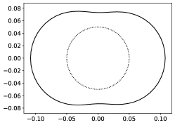
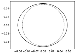
Figure 2. $T_{\text{euclid}}$ (left), $T_{\text{sobolev}}$ (middle), and $T_{\text{witten}}$ (right).

First, consider the plot of $T_{\text{euclid}}$ in Figure 2. Since the probability measures $f$ and $f_{\varepsilon v}$ are probability densities, they can be thought of as being normalized to have $L^{1}$-norm equal to $1$, which is the reason that the scale of $T_{\text{euclid}}$ is much larger than $\varepsilon S$ which appears as a dot. The shape of $T_{\text{euclid}}$ can be interpreted as follows: if the image $f$ is translated up, then the vertical stripes will mostly overlap, see Figure 1, resulting in a small change in the Euclidean distance. In contrast, if the image is shifted left, then the strips will become misaligned resulting in a large change in the Euclidean distance; this explains the barbell shape of the set $T_{\text{euclid}}$. Next, consider the plot of $T_{\text{sobolev}}$ in Figure 2 corresponding to the unweighted Sobolev norm, which partially corrects the scaling. Finally, the plot of $T_{\text{wittin}}$ which is the linear approximation of Wasserstein distance computed using the method described in this paper nearly recovers the circle with only a small deformation.

5.5. Numerical example: visualizing effect of changing variance

In this section, we again visualize how different metrics compare to $W_{2}$ by considering a subset of the sphere $\{\nu:W_{2}(\mu,\nu)=\varepsilon\}$. By assuming that the density $f$ of $\mu$ is a Gaussian function with a diagonal covariance matrix we can consider the subset of $\{\nu:W_{2}(\mu,\nu)=\varepsilon\}$ consisting of Gaussian distributions with the same mean, but whose diagonal covariance matrix is different. Let $f$ be a Gaussian function centered at $(1/2,1/2)^{\top}$ with diagonal covariance matrix $\Sigma_{f}=\operatorname{diag}(\sigma_{f}^{2})$ where $\sigma_{f}^{2}=(\sigma_{f,1}^{2},\sigma_{f,2}^{2})$

$$f(x):=\frac{1}{2\pi(\det\Sigma_{f})^{1/2}}\exp\left(-\frac{1}{2}(x-(1/2,1/2)^{\top})^{\top}\Sigma_{f}^{-1}(x-(1/2,1/2)^{\top})\right).$$

We plot $f$ and its regularized potential $V_{\tau}$ in Figure 3.

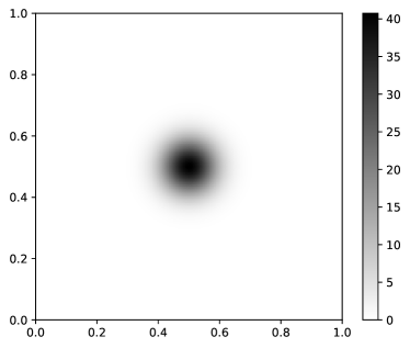
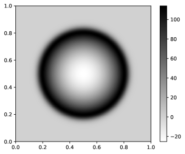
Figure 3. The function $f$ (left) and its regularized potential $V_{\tau}$ (right).

If the density $g$ of $\nu$ is the Gaussian function centered at $(1/2,1/2)^{\top}$ with diagonal covariance matrix $\Sigma_{g}=\operatorname{diag}(\sigma_{g}^{2})$, then recall that by (30) we have

(36) $$W_{2}(\mu,\nu)=|\sigma_{f}-\sigma_{g}|.$$

Fix $\varepsilon>0$, let $S$ denote the unit circle $S:=\{v\in\mathbb{R}^{2}:\|v\|_{2}=1\}$, and observe that

(37) $$\left\{W_{2}(\mu,\mu_{\varepsilon v})v\in\mathbb{R}^{2}:v\in S\right\}=\varepsilon S,$$

where here $\mu_{\varepsilon v}$ is the measure with density $f_{\varepsilon v}$, where $f_{\varepsilon v}$ is a Gaussian function centered at the $(1/2,1/2)^{\top}$ with diagonal covariance

$$\Sigma_{f_{\varepsilon v}}=\operatorname{diag}((\sigma_{f}+\varepsilon v))^{2}.$$

That is, $f_{\varepsilon v}$ changes the standard deviations $\sigma_{f}$ of the Gaussian $f$ by $\varepsilon v$. The fact that (37) holds follows from (36). As in the previous section, we study analogs of the set defined in the left hand side of (37), where the $W_{2}$ metric is replaced by our linearization, the unweighted Sobolev norm, and the Euclidean norm, respectively. In particular, we define

$$V_{\text{witten}}:=\left\{\|(f-f_{\varepsilon v})/f_{\tau}\|_{\dot{H}^{-1}(d\mu_{\tau})}v\in\mathbb{R}^{2}:v\in S\right\},$$

$$V_{\text{sobolev}}:=\left\{\|f-f_{\varepsilon v}\|_{\dot{H}^{-1}(dx)}v\in\mathbb{R}^{2}:v\in S\right\},$$

and

$$V_{\text{euclid}}:=\left\{\|f-f_{\varepsilon v}\|_{L^{2}(dx)}v\in\mathbb{R}^{2}:v\in S\right\}.$$

We plot the sets $V_{\text{witten}},V_{\text{sobolev}},$ and $V_{\text{euclid}}$ in Figure 2. Note that the set $\varepsilon S$ is included for reference and is plotted using a dotted line in the plots of Figure 2.

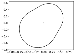
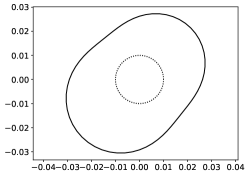
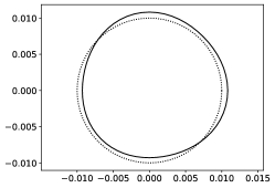
Figure 4. $V_{\text{euclid}}$ (left), $V_{\text{sobolev}}$ (middle), and $V_{\text{witten}}$ (right).

First, observe that the plots of $V_{\text{euclid}}$ and $V_{\text{sobolev}}$ in Figure 4 appear stretched in the $(1,1)$ and $(-1,-1)$ directions: when the vector $\varepsilon v$ changing the standard deviations is in the positive quadrant this corresponds to increasing the standard deviation of both variables. Similarly, the negative quadrant (where both components of $v$ are negative) corresponds to decreasing the standard deviation of both variables. Both of these deformations result in a similarly large change. In contrast, the other quadrants (where the components of $v$ have different signs) correspond to increasing one standard deviation in one direction while decreasing the standard deviation in the other direction; this explains the asymmetry of $V_{\text{euclid}}$ and $V_{\text{sobolev}}$. In contrast, the plot of $V_{\text{witten}}$ in Figure 4 roughly preserves the circle with only a small deformation.

5.6. Numerical example: managing noise and computational cost

In this section, we remark how the method can be used in more practical situations involving images. In particular, we consider a $129\times 129$ image containing a biomolecule. In order to manage both the computational cost and noise, we define the potential $V_{\tau}$ with $\tau=0.01$, see Figure 5.

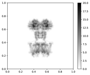
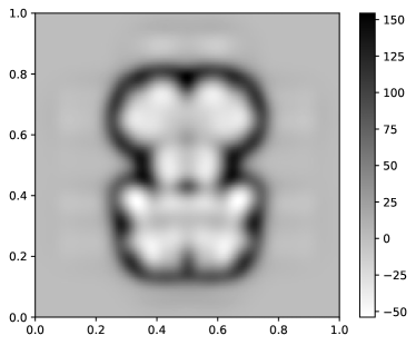
Figure 5. Function $f$ (left) and its regularized potential $V$ (right)

Observe that the maximum value of the potential in Figure 5 is about 150. Therefore, we expect the computational cost to be proportional to the square root of $150$. Using Algorithm 5.1 to compute distances based on this image has an average time of about $0.035\text{ (seconds) }$ on a laptop, where the average is taken over $128$ computations.

5.7. Numerical example: local embedding

In this section, we discuss an immediate extension of the described method to defining an embedding of the negative weighted homogeneous Sobolev norm. In particular, we can define a map

$$g\mapsto\Phi_{f}(g)$$

such that

(38) $$\|\Phi_{f}(g)-\Phi_{f}(h)\|_{L^{2}}=\|g-h\|_{\dot{H}^{-1}(d\mu)}.$$

Indeed, it follows from §3.4 that if

$$\Phi_{f}(g)=H^{-1/2}((f-g)/\sqrt{f}),$$

where $H=-\Delta+V$ and the potential $V$ depends on $f$, then (38) holds. The operator $H^{-1/2}$ with Neumann boundary conditions is well defined since $H$ is positive definite on a subspace that contains $(f-g)/\sqrt{f}$. Computationally, $H^{-1/2}$ can be computed using a version of $H$ with a regularized potential via an iterative method based on approximating $\sqrt{x}$ by Chebyshev polynomials. To illustrate this embedding we define Gaussian functions $f,g,h$ with means

$$\mu_{f}=(1/2,1/2),\quad\mu_{g}=\mu_{f}+(0.001,0.002),\quad\mu_{h}=\mu_{f}+0.003,-0.002)$$

and standard deviations

$$\sigma_{f}=(1/16,1/14),\quad\sigma_{g}=\sigma_{f}+(0.001,0.003),\quad\sigma_{h}=\sigma_{f}+(-0.001,0.002),$$

respectively, where the Gaussian function is defined by (32). We compute $\Phi_{f}(g)$ and $\Phi_{f}(h)$ and plot the result in Figure 6.

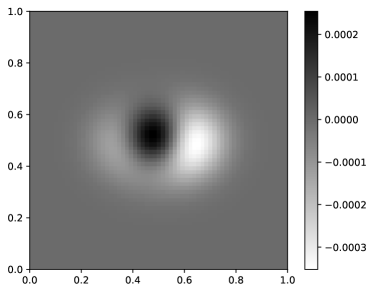
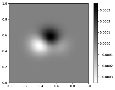
Figure 6. $\Phi_{f}(g)$ (left) and $\Phi_{f}(h)$ (right).

We find that

$$\|\phi_{f}(g)-\phi_{f}(h)\|_{L^{2}}=4.949\times 10^{-3},$$

and using the analytic formula for the $W_{2}$ metric between these Gaussian distributions gives

$$|\|\phi_{f}(g)-\phi_{f}(h)\|_{L^{2}}-W_{2}(\nu,\eta)|\approx 5.080\times 10^{-5}$$

where $\mu$ and $\eta$ are the measures associated with $g$ and $h$, respectively, which verifies the effectiveness of this embedding as a local approximation of the $W_{2}$ metric.

6. Discussion

In this paper we have studied a classic linearization of Wasserstein distance. In particular, we focused on the connection between $W_{2}$ and the Witten Laplacian which is a Schrödinger operator of the form

$$H=-\Delta+V.$$

From a computational point of view, the principle advantage of this formulation is that the computational cost of solving $H=-\Delta+V$ can be roughly bounded by the square root of the maximum value of the potential (since this influences the condition number of solving $H\psi=u$ after an appropriate transformation). The potential $V$ can be smoothed until an acceptable computational cost is achieved. For example, if the maximum value of $V$ is $100$, then the number of iterations for Conjugate Gradient will be $\sim 10$, where each iteration has the same cost of computing the unweighted Sobolev norm. The numerical experiments indicate how this Witten Laplacian distance will, roughly speaking, preserve the Wasserstein distance for small balls around measures. This perspective opens the possibility of many interesting applications. For example, the operator $H$ can be used to smooth images via the diffusion

$$f\mapsto\exp(-\tau H)f,$$

where $\exp$ denotes the operator exponential, which is interesting since the infinitesimal generator $H$ of the diffusion has a connection to Wasserstein distance. More generally, the fractional diffusion

$$f\mapsto\exp(-\tau H^{\alpha})f,$$

for $\alpha>0$ can be considered where $H^{\alpha}$ is the operator to power $\alpha$, which is well defined since $H$ is positive semi definite. There are other interesting applications about defining embeddings into Euclidean space, and potential applications to graphs. Another potential application is related to maximum mean discrepancy (MMD), which has been consider by other authors, see the discussion in §1.3, but our perspective may offer some new ideas.

References

- [1] Michael Arbel, Anna Korba, Adil Salim, and Arthur Gretton, Maximum mean discrepancy gradient flow., NeurIPS, 2019, pp. 6481–6491.
- [2] Jean-David Benamou and Yann Brenier, A computational fluid mechanics solution to the monge-kantorovich mass transfer problem, 84 (2000), no. 3, 375–393.
- [3] Brenier, Y. Decomposition polaire et rearrangement monotone des champs de vecteurs. C.R. Acad. Sci. Paris, Serie I, 305 (1987), 805-808.
- [4] Clément Cancès, Thomas O. Gallouët, and Gabriele Todeschi, A variational finite volume scheme for wasserstein gradient flows, Numerische Mathematik 146 (2020), no. 3, 437–480.
- [5] Hong-Bin Chen and Jonathan Niles-Weed, Asymptotics of smoothed wasserstein distances, Potential Analysis (2021).
- [6] Bruno Colbois, Ahmad El Soufi, and Alessandro Savo, Eigenvalues of the laplacian on a compact manifold with density, 2013.
- [7] Jean Dolbeault, Bruno Nazaret, and Giuseppe Savaré, A new class of transport distances between measures, 34 (2008), no. 2, 193–231.
- [8] Matthew M. Dunlop and Yunan Yang, Stability of gibbs posteriors from the wasserstein loss for bayesian full waveform inversion, SIAM/ASA Journal on Uncertainty Quantification 9 (2021), no. 4, 1499–1526.
- [9] Björn Engquist, Kui Ren, and Yunan Yang, The quadratic wasserstein metric for inverse data matching, 36 (2020), no. 5, 055001.
- [10] Björn Engquist and Yunan Yang, Optimal transport based seismic inversion:beyond cycle skipping, Communications on Pure and Applied Mathematics (2021).
- [11] David Gilbarg and Neil S. Trudinger, Elliptic partial differential equations of second order, Springer Berlin Heidelberg, 2001.
- [12] Kantorovich, L. V. On the translocation of masses. C. R. (Dokl.) Acad. Sci. URSS 37 (1942), 199-201.
- [13] Mikhail Karpukhin, Mickaël Nahon, Iosif Polterovich, and Daniel Stern, Stability of isoperimetric inequalities for laplace eigenvalues on surfaces, 2021.
- [14] Frédéric De Gournay, Jonas Kahn, Léo Lebrat, and Pierre Weiss, Optimal Transport Approximation of 2-Dimensional Measures, SIAM Journal on Imaging Sciences (2019).
- [15] Michel Ledoux and Jie-Xiang Zhu, On optimal matching of gaussian samples III, Probability and Mathematical Statistics 41 (2020), no. 2.
- [16] P. L. Lions, Two remarks on monge-ampere equations, Annali di Matematica Pura ed Applicata 142 (1985), no. 1, 263–275.
- [17] P.-L. Lions, N. S. Trudinger, and J. I. E. Urbas, The neumann problem for equations of monge-ampère type, Communications on Pure and Applied Mathematics 39 (1986), no. 4, 539–563.
- [18] Monge, G. Memoire sur la theorie des deblais et des remblais. In Histoire de l’Academie Royale des Sciences de Paris (1781), pp. 666-704.
- [19] Youssef Mroueh, Tom Sercu, and Anant Raj, Sobolev descent, Proceedings of the Twenty-Second International Conference on Artificial Intelligence and Statistics, Proceedings of Machine Learning Research, vol. 89, PMLR, 2019, pp. 2976–2985.
- [20] Sloan Nietert, Ziv Goldfeld, and Kengo Kato, Smooth -wasserstein distance: Structure, empirical approximation, and statistical applications, Proceedings of the 38th International Conference on Machine Learning , Proceedings of Machine Learning Research, vol. 139, PMLR, 18–24 Jul 2021, pp. 8172–8183
- [21] F. Otto and C. Villani, Generalization of an inequality by talagrand and links with the logarithmic sobolev inequality, Journal of Functional Analysis 173 (2000), no. 2, 361–400.
- [22] Gabriel Peyré and Marco Cuturi, Computational optimal transport, Foundations and Trends in Machine Learning 11 (2019), no. 5-6, 355–607.
- [23] Rémi Peyre, Comparison between distance and norm, and localisation of wasserstein distance, 2016.
- [24] Eigenvalue estimates for the weighted Laplacian on a Riemannian manifold by Setti (1998).
- [25] Santambrogio, F. Optimal transport for applied mathematicians: calculus of variations, PDEs, and modeling, Birkhauser, 2015.
- [26] Stefan Steinerberger, A Wasserstein inequality and minimal Green energy on compact manifolds, Journal of Functional Analysis 281 (2021), no. 5, 109076.
- [27] Stefan Steinerberger, Wasserstein distance, fourier series and applications, Monatshefte für Mathematik 194 (2021), no. 2, 305–338.
- [28] Neil S. Trudinger and Xu-Jia Wang, The Monge-Ampère equation and its geometric applications, Handbook of geometric analysis. No. 1, Adv. Lect. Math. (ALM), vol. 7, Int. Press, Somerville, MA, 2008, pp. 467–524.
- [29] Cédric Villani, Topics in optimal transportation, Graduate Studies in Mathematics, vol. 58, American Mathematical Society, Providence, RI, 2003. MR 1964483
- [30] Max-K. von Renesse and Karl-Theodor Sturm, Transport inequalities, gradient estimates, entropy and ricci curvature, Communications on Pure and Applied Mathematics 58 (2005), no. 7, 923–940.
- [31] Yunan Yang, Jingwei Hu, and Yifei Lou, Implicit regularization effects of the sobolev norms in image processing, 2021.