Evidence of two-spinon bound states in the magnetic spectrum of Ba₃CoSb₂O₉

Abstract

Recent inelastic neutron scattering (INS) experiments of the triangular antiferromagnet Ba₃CoSb₂O₉ revealed strong deviations from semiclassical theories. We demonstrate that key features of the INS data are well reproduced by a parton Schwinger boson theory beyond the saddle-point approximation. The measured magnon dispersion is well reproduced by the dispersion of two-spinon bound states (poles of the emergent gauge fields propagator), while the low-energy continuum scattering is reproduced by a quasifree two-spinon continuum, suggesting that a free spinon gas is a good initial framework to study magnetically ordered states near a quantum melting point.

I Introduction

Identifying new states of matter is a central theme of condensed matter physics. Although theorists have predicted an abundance of such states, it is often difficult to find experimental realizations. This is particularly a challenge for quantum spin liquids (QSLs), where the lack of smoking-gun signatures is forcing the community to develop more comprehensive approaches Knolle and Moessner (2019); Broholm et al. (2020); Savary and Balents (2016). The singular interest in the fractionalized quasi-particles of these highly entangled states of matter resides in their potential application to quantum information Kitaev (2003); Broholm et al. (2020); Tokura et al. (2017). However, it has been frustratingly difficult to detect these quasiparticles in real materials.

Since Anderson’s proposal of the resonating valence bond state Anderson (1973), the triangular geometry has long been studied as a platform for finding QSLs. Although the ground state of the simplest spin-$1/2$ model with nearest-neighbor (NN) antiferromagnetic Heisenberg interactions $J_{1}$ exhibits a $120^{\circ}$ long-range magnetic order, geometric frustration makes this order weak Capriotti et al. (1999); White and Chernyshev (2007). Indeed, a next-nearest-neighbor exchange coupling $J_{2}$ as small as $\approx 0.06J_{1}$ is enough to continuously melt the magnetic order into a QSL phase Hu et al. (2015); Iqbal et al. (2016); Saadatmand and McCulloch (2016); Wietek and Läuchli (2017); Gong et al. (2017); Hu et al. (2019); Zhu and White (2015); Zhu et al. (2018). Determining the nature of the QSL is an ongoing theoretical challenge, with proposals ranging from gapped $\mathbb{Z}_{2}$ and gapless $U(1)$ Dirac to chiral Zhu and White (2015); Hu et al. (2015); Iqbal et al. (2016); Saadatmand and McCulloch (2016); Wietek and Läuchli (2017); Gong et al. (2017); Hu et al. (2019). To discern among QSL candidates and the corresponding low-energy parton theories, it is imperative to make contact with experiments. Since most of the known realizations of the triangular lattice Heisenberg antiferromagnet (TLHA) lie on the ordered side of the quantum critical point (QCP) at $J_{2}/J_{1}\approx 0.06$ Manuel and Ceccatto (1999); Mishmash et al. (2013); Kaneko et al. (2014); Li et al. (2015); Zhu and White (2015); Zhu et al. (2018), reproducing their measured excitation spectrum is the most stringent test for alternative parton theories.

The idea of describing two-dimensional (2D) frustrated antiferromagnets by means of fractional excitations (spinons) coupled to emergent gauge fields has been around for many years Arovas and Auerbach (1988); Sachdev and Read (1991); Read and Sachdev (1991); Chubukov et al. (1994); Chubukov and Starykh (1996). The Schwinger boson theory (SBT) is one of the first parton formulations that was introduced to describe ordered and disordered phases on an equal footing  Auerbach (1994); Read and Sachdev (1991). However, a qualitatively correct, beyond the saddle-point (SP) level, computation of the dynamical structure factor of magnetically ordered phases has been achieved only recently Ghioldi et al. (2018); Zhang et al. (2019, 2021), enabling comparisons with inelastic neutron scattering (INS) measurements.

Ba₃CoSb₂O₉ is one of the best known realizations of a spin-$1/2$ TLHA Macdougal et al. (2020); Zhou et al. (2012); Ito et al. (2017); Ma et al. (2016). INS studies of this material Ma et al. (2016); Ito et al. (2017); Macdougal et al. (2020) reveal an unusual three-stage energy structure of the magnetic spectral weight [see Fig. 2(a)]. The lowest-energy stage is composed of dispersive branches of single-magnon excitations. The second and third stages correspond to dispersive continua that extend up to energies six times larger than the single-magnon bandwidth Ito et al. (2017). These observations are quantitatively and qualitatively inconsistent with nonlinear spin wave theory (NLSWT) Ma et al. (2016); Kamiya et al. (2018), suggesting that magnons could be better described as two-spinon bound states (spinons are the fractionalized quasiparticles of the neighboring QSL state). Here we investigate this hypothesis by comparing the INS data of Ba₃CoSb₂O₉ Ito et al. (2017); Macdougal et al. (2020) against the SBT described in Refs. Ghioldi et al. (2018); Zhang et al. (2019, 2021).

These comparisons demonstrate that a low-order SBT provides an adequate starting point to reproduce the measured spectrum of low-energy excitations, including the magnon dispersion (first stage) reported in Ref. Macdougal et al. (2020) and the dispersion of the broad low-energy peak that appears in the continuum (second stage) Ito et al. (2017); Macdougal et al. (2020). Importantly, these results shed light on the nature of the proximate QCP and of the quantum spin liquid phase that is expected for $J_{2}/J_{1}\gtrsim 0.06$ Scheie et al. (2021).

II Material and Model

Ba₃CoSb₂O₉ comprises vertically stacked triangular layers of effective spin-1/2 moments arising from the $\mathcal{J}=1/2$ Kramers doublet of Co²⁺ in a trigonally-distorted octahedral ligand field. Excited multiplets are separated by a gap of 200-300 K due to spin-orbit coupling, which is much larger than the Néel temperature $T_{\text{N}}=3.8$ K. Below $T_{\text{N}}$, the material develops conventional 120^∘ ordering with wavevector $\mathbf{Q}=(1/3,1/3,1)$ Doi et al. (2004). The theoretical modeling of different experimental results Susuki et al. (2013); Koutroulakis et al. (2015); Ma et al. (2016); Kamiya et al. (2018) indicates that the magnetic properties of Ba₃CoSb₂O₉ are well described by the XXZ model:

$${\mathcal{H}}=\sum_{\langle{i,j}\rangle}J_{ij}\left(S^{x}_{i}S^{x}_{j}+S^{y}_{i}S^{y}_{j}+\Delta S^{z}_{i}S^{z}_{j}\right),$$ (1)

where $\langle i,j\rangle$ restricts the sum to NN intralayer and interlayer bonds with exchange interactions $J_{ij}=J$ and $J_{ij}=J_{c}$, respectively, and $\Delta$ accounts for a small easy plane exchange anisotropy  . Since the set of in-plane Hamiltonian parameters reported in Refs. Ito et al. (2017); Macdougal et al. (2020); Kamiya et al. (2018) coincide with each other within a relative error $\sim 5\%$, here we adopt the values $J=1.66$ meV and $\Delta=0.937$. As for the inter-plane exchange, we adopt $J_{c}=0.061J$, between the values $J_{c}=0.05J$ and $J_{c}=0.08J$ reported in Refs. Kamiya et al. (2018) and Ito et al. (2017); Macdougal et al. (2020), respectively. As expected for this effective spin model, experiments confirmed a one-third magnetization plateau (up-up-down phase) induced by a magnetic field parallel to the easy-plane Chubukov and Golosov (1991); Shirata et al. (2012); Susuki et al. (2013); Koutroulakis et al. (2015); Quirion et al. (2015); Sera et al. (2016). While the dynamical spin structure factor of the up-up-down phase is well described by NLSWT Alicea et al. (2009); Kamiya et al. (2018), the observed zero-field magnon dispersions cannot be described with any known semiclassical treatment Ma et al. (2016); Ito et al. (2017), suggesting that quantum renormalization effects in the zero field are underestimated by a perturbative $1/S$ expansion. These strong quantum fluctuations can be attributed to the proximity of the TLHA to the above-mentioned “quantum melting point” that signals a continuous $T=0$ transition into a quantum spin liquid.

III Schwinger Boson Theory

The SBT Arovas and Auerbach (1988); Auerbach (1994); Ghioldi et al. (2018) starts from a parton representation of the spin operators expressed in terms of spin-$1/2$ bosons that represent the spinons of the theory: $\hat{\boldsymbol{S}}_{i}=\frac{1}{2}{\boldsymbol{b}}_{i}^{{\dagger}}{\boldsymbol{\sigma}}{\boldsymbol{b}}_{i}$, where ${\boldsymbol{b}}_{i}^{{\dagger}}=(b_{i\uparrow}^{{\dagger}},\ b_{i\downarrow}^{{\dagger}})$, and ${\boldsymbol{\sigma}}\equiv(\sigma^{x},\ \sigma^{y},\ \sigma^{z})$ is the vector of Pauli matrices. The spin-$1/2$ representation of the spin operator is enforced by the constraint $\sum_{\sigma=\uparrow,\downarrow}b_{i\sigma}^{{\dagger}}b_{i\sigma}=1$. The advantage of this representation is that the spin-spin interaction can be expressed as a bilinear form, $X^{\dagger}_{ij}X_{ij}$, in bond operators $X_{ij}$ which are invariant under the spin-rotation symmetries of the Hamiltonian. Correspondingly, the mean-field approximation $X^{\dagger}_{ij}X_{ij}\simeq\langle X^{\dagger}_{ij}\rangle X_{ij}+X^{\dagger}_{ij}\langle X_{ij}\rangle-\langle X^{\dagger}_{ij}\rangle\langle X_{ij}\rangle$ preserves the rotational symmetry of the spin Hamiltonian. This is one of the important differences between SBT and spin wave theory Arovas and Auerbach (1988); Auerbach (1994).

For the case of interest, the XXZ interaction [Eq. (1)] can be expressed in terms of SU(2) spin-rotation invariant bond operators Ghioldi et al. (2015), $A_{ij}=\frac{1}{2}(b_{i\uparrow}b_{j\downarrow}-b_{i\downarrow}b_{j\uparrow})$, $B_{ij}=\frac{1}{2}(b_{j\uparrow}^{{\dagger}}b_{i\uparrow}+b_{j\downarrow}^{{\dagger}}b_{i\downarrow})$, and U(1) spin-rotation invariant bond operators $C_{ij}=\frac{1}{2}(b_{j\uparrow}^{{\dagger}}b_{i\uparrow}-b_{j\downarrow}^{{\dagger}}b_{i\downarrow})$ and $D_{ij}=\frac{1}{2}(b_{i\uparrow}b_{j\downarrow}+b_{i\downarrow}b_{j\uparrow})$ required to account for the finite uniaxial anisotropy. The operator $A^{\dagger}_{ij}$ ($D^{\dagger}_{ij}$) creates a singlet (triplet) state on the bond $ij$. The operator $B_{jk}$ moves singlets and triplets from the bond $ij$ to the bond $ik$ preserving their character. In contrast, the operator $C_{jk}$ promotes a singlet bond $ij$ into a triplet bond $ik$, and vice versa. Up to an irrelevant constant, the spin-spin interaction is expressed as Scheie et al. (2021)

$$S^{x}_{i}S^{x}_{j}+S^{y}_{i}S^{y}_{j}+\Delta S^{z}_{i}S^{z}_{j}=-2\left(\frac{\Delta+1}{2}-\alpha\right)A_{ij}^{{\dagger}}A_{ij}$$

$$+2\alpha:\!B_{ij}^{{\dagger}}B_{ij}\!:+\frac{\Delta-1}{2}\;(:\!C_{ij}^{{\dagger}}C_{ij}\!:-D_{ij}^{{\dagger}}D_{ij}).$$ (2)

The continuous parameter $\alpha$ parameterizes equivalent ways of expressing the spin-spin interaction by assigning different weights to $A_{ij}^{{\dagger}}A_{ij}$ and $:\!B_{ij}^{{\dagger}}B_{ij}\!:$. This parametrization leads to a family of possible mean-field solutions in the canonical formalism or Hubbard-Stratonovich transformations in the path-integral formulation. Similarly to the case of KYbSe₂ Scheie et al. (2021), the optimal value of $\alpha$ is obtained by fitting the INS data. We note, however, that the present SBT recovers the exact dynamical structure factor (LSWT result) in the large-$S$ limit for any value of $\alpha$ Zhang et al. (2021). Following the procedure described in Ref. Ghioldi et al., 2018, we use the path-integral formulation. The auxiliary field $\lambda$ is introduced to enforce the constraint $\sum_{\sigma=\uparrow,\downarrow}b_{i\sigma}^{{\dagger}}b_{i\sigma}=1$. To decouple the bilinear forms $\bar{X}X$ in Eq. (2), we perform a Hubbard-Stratonovich transformation,

$$e^{\rm{sgn}(J_{ij})|J_{ij}|\overline{X}_{ij}X_{ij}} =|J_{ij}|\int\frac{d\overline{W}_{ij}^{X}\ dW_{ij}^{X}}{2\pi i}e^{-|J_{ij}|\overline{W}_{ij}^{X}W_{ij}^{X}}$$

$$\times e^{|J_{ij}|\big{(}\rm{sgn}(J_{ij})\overline{W}_{ij}^{X}X_{ij}+W_{ij}^{X}\overline{X}_{ij}\big{)}},$$ (3)

where $W^{X}_{ij}$ with $X=A,B,C,$ and $D$ are the Hubbard-Stratonovich fields. The complex SB or spinon field $b$ can be formally integrated out, and the exact partition function is expressed as a path integral over the auxiliary fields $W^{X}$ and $\lambda$,

$$\mathcal{Z}[j]=\int[D\overline{W}DW][D\lambda]\ e^{-S_{\rm eff}(\overline{W},W,\lambda,j,h)}.$$ (4)

The source $j$ couples the system with a general external magnetic field and it is used to compute correlation functions. The Lagrange multiplier $\lambda$ and the phases of the auxiliary fields $W^{X}$ are the emergent gauge fields of the SBT Ghioldi et al. (2018). The magnetic ordering emerges as a spontaneous Bose-Einstein condensation of the spinon field. Since the Hubbard-Stratonovich transformation does not break the U(1) symmetry of ${\mathcal{H}}$, an infinitesimal symmetry-breaking field $h$ is necessary to select a condensate associated with a particular choice of the 120^∘ ordering (vector chirality and orientation of the ordered moment of a given spin). The effective action can be divided into two contributions: $S_{\rm{eff}}(\overline{W},W,\lambda,j,h)=S_{0}(\overline{W},W,\lambda)+S_{\rm bos}(\overline{W},W,\lambda,j,h)$, with

$$S_{0}({\overline{W}},W,\lambda)=\!\!\int_{0}^{\beta}\!\!d\tau\big{(}\sum\limits_{ij,X}\!J_{ij}{\overline{W}}_{ij}^{X\tau}W_{ij}^{X\tau}\!\!-\!\!i2S\sum_{i}\!\lambda_{i}^{\tau}\big{)},$$ (5)

and

$$S_{\rm bos}(\overline{W},W,\lambda,j,h) =-\frac{1}{2}{\rm ln}\int D[\bar{b},b]\ e^{-\boldsymbol{b}^{\dagger}\mathcal{M}\ \boldsymbol{b}}$$

$$=\frac{1}{2}{\rm Tr}\ {\rm ln}\Big{[}\mathcal{G}^{-1}(\overline{W},W,\lambda,j,h)\Big{]},$$ (6)

where $\boldsymbol{b}$ is the complex Nambu spinor field, $\beta=1/k_{B}T$, $\mathcal{G}\!=\!\mathcal{M}^{-1}$ is the single-spinon propagator, $\mathcal{M}$ is the bosonic dynamical matrix, and the trace is taken over space, time, and boson indices. The next step is to expand the effective action around its saddle-point (SP) solution (equivalent to the mean-field solution in the canonical formalism),

$$S_{\rm eff}=S_{\rm eff}^{\rm sp}+\sum S_{\alpha_{1}\alpha_{2}}^{(2)}\Delta\phi_{\alpha_{1}}\Delta\phi_{\alpha_{2}}+S_{\rm int},$$ (7)

where $S_{\rm eff}^{\rm sp}$ is the value of the effective action at the SP solution $\phi^{sp}_{\alpha}$: $\partial S_{\rm eff}/\partial\phi_{\alpha}|_{\rm sp}=0$, with $\phi_{\alpha}\equiv(\overline{W}_{ij}^{X},\ W_{ij}^{X},\ \lambda_{i})$. The second term is the Gaussian contribution determined by the fluctuation matrix $S_{\alpha_{1}\alpha_{2}}^{(2)}\!=\!\frac{1}{2}\left(\partial^{2}S_{\rm eff}/\partial\phi_{\alpha_{1}}\partial\phi_{\alpha_{2}}\right)|_{\rm sp}$ and $\Delta\phi_{\alpha}=\phi_{\alpha}-\phi^{\rm sp}_{\alpha}$. The third term $S_{\rm int}=\sum_{n=3}^{\infty}\sum_{\alpha_{1}\cdots\alpha_{n}}S_{\alpha_{1}\cdots\alpha_{n}}^{(n)}\Delta\phi_{\alpha_{1}}\cdots\Delta\phi_{\alpha_{n}}$, with $S_{\alpha_{1}\cdots\alpha_{n}}^{(n)}\!=\!\frac{1}{n!}\left(\partial^{n}S_{\rm eff}/\partial\phi_{\alpha_{1}}\cdots\partial\phi_{\alpha_{n}}\right)|_{\rm sp}$, includes higher-order terms in the fluctuations of the auxiliary fields.

At the SP or mean-field level, the auxiliary fields $\lambda_{i}$ and $W_{ij}^{X}$ are uniform and static. Correspondingly, the mean-field theory describes a noninteracting gas of SBs or spin-$1/2$ spinons with a free-spinon propagator $\mathcal{G}^{\rm{sp}}$. The resulting condensation of these spinons at $T\leq T_{N}$ leads to 120^∘ magnetic ordering within each triangular layer and antiferromagnetic ordering between adjacent layers Arovas and Auerbach (1988); Auerbach (1994); Ghioldi et al. (2015). Correspondingly, the free spinon propagator acquires a new contribution from the condensate. Furthermore, as it was shown in recent works Ghioldi et al. (2018); Zhang et al. (2019), fluctuations of the auxiliary fields mediate spinon-spinon interactions that drastically modify the nature of the low-energy spin excitations revealed by the dynamical spin susceptibility in Matsubara frequency $i\omega$ and momentum $\boldsymbol{q}$ space:

$$\chi_{\mu\nu}(\boldsymbol{q},i\omega)=\lim_{h\rightarrow 0}\lim_{N_{s}\rightarrow\infty}\frac{\partial^{2}ln\mathcal{Z}[j]}{\partial j_{\boldsymbol{q},i\omega}^{\ \mu}\ \partial j_{-\boldsymbol{q},-i\omega}^{\ \nu}}\bigg{|}_{j=0},$$ (8)

where $\mu,\nu=x,y,z$ and $N_{s}$ is the total number of spins.

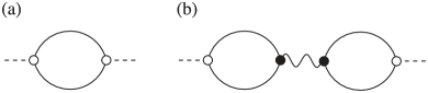
Figure 1: Diagrammatic representation of different contributions to the dynamical spin susceptibility: (a) saddle-point and (b) Gaussian fluctuations around the SP solution Ghioldi et al. (2018); Zhang et al. (2021). The dashed lines represent the external fields. The full lines represent the single-spinon propagator for the SP solution. The wavy lines represent the propagator of the auxiliary fields Auerbach (1994), whose poles correspond to the true magnons of the SBT.

By following the procedure described in detail in Ref. Ghioldi et al., 2018, we compute the $1/N$ correction ($N$ is the number of bosonic flavors) by including the Gaussian fluctuations of the auxiliary fields $W^{X}$ and $\lambda$. At this level, the resulting dynamical spin susceptibility takes the form

$$\chi_{\mu\nu}(\boldsymbol{q},i\omega)=\chi_{\mu\nu}^{\rm sp}(\boldsymbol{q},i\omega)+\chi_{\mu\nu}^{\rm fl}(\boldsymbol{q},i\omega),$$ (9)

where

$$\chi_{\mu\nu}^{\rm{sp}}(\boldsymbol{q},i\omega)=\frac{1}{2}{\rm Tr}\left[\mathcal{G}^{\rm{sp}}u^{\mu}(\boldsymbol{q},i\omega)\mathcal{G}^{\rm{sp}}u^{\nu}(-\boldsymbol{q},-i\omega)\right],$$ (10)

denotes the contribution obtained at the saddle-point level, and

$$\chi_{\mu\nu}^{\rm fl}(\boldsymbol{q},i\omega)=\sum_{\alpha_{1}\alpha_{2}} \frac{1}{2}{\rm Tr}\big{[}\mathcal{G}^{\rm sp}\ v_{\phi_{\alpha_{1}}}\ \mathcal{G}^{\rm sp}\ u^{\mu}(\boldsymbol{q},i\omega)\big{]}$$

$$\times D_{\alpha_{1}\alpha_{2}}(\boldsymbol{q},i\omega) \frac{1}{2}{\rm Tr}\big{[}\mathcal{G}^{\rm sp}\ v_{\phi_{\alpha_{2}}}\ \mathcal{G}^{\rm sp}\ u^{\nu}(-\boldsymbol{q},-i\omega)\big{]}.$$ (11)

is the contribution from Gaussian fluctuations around the saddle-point solution. The propagator of the auxiliary fields $D_{\alpha_{1}\alpha_{2}}(\boldsymbol{q},i\omega)$ (also known as random phase approximation (RPA) propagator) is the inverse of the fluctuation matrix $S_{\alpha_{1}\alpha_{2}}^{(2)}$. The internal and external vertices, $v_{{\phi}_{\alpha}}\!=\!{\partial\mathcal{G}^{-1}}/{\partial\phi_{\alpha}}$ and $u^{\mu}(\boldsymbol{q},i\omega)\!=\!\partial\mathcal{G}^{{}^{-1}}\!/\partial j_{\boldsymbol{q},i\omega}^{\;\mu}$, couple the spinons to the auxiliary fields $\phi_{\alpha}$ and to the external fields, respectively. The contributions $\chi_{\mu\nu}^{\rm sp}(\boldsymbol{q},i\omega)$ and $\chi_{\mu\nu}^{\rm fl}(\boldsymbol{q},i\omega)$ are represented as Feynman diagrams in Figs. 1(a) and 1(b), respectively.

Historically, the community working on SBT tried to fit experimental results using the mean field susceptibility $\chi^{\rm{sp}}_{\mu\nu}(\boldsymbol{q},i\omega)$  Auerbach and Arovas (1988); Fåk et al. (2012); Ghioldi et al. (2015); Samajdar et al. (2019). However, the poles of $\chi^{\rm{sp}}_{\mu\nu}(\boldsymbol{q},i\omega)$ coincide with the poles of the single-spinon propagator $\mathcal{G}^{\rm sp}$ (single-spinon poles). As we demonstrated in Refs. Ghioldi et al., 2018; Zhang et al., 2019, 2021, the true collective modes (magnons) of the magnetically ordered state arise as two spinon-bound states associated with poles of the propagator of the auxiliary fields. Correspondingly, the magnons of the theory can only be obtained by including contributions from fluctuations around the SP solution. As it is discussed in Ref. Zhang et al., 2021, for each diagram of the $1/N$ expansion of the dynamical spin susceptibility, there is a counter-diagram that cancels the residues of the unphysical single-spinon poles. In particular, the counter-diagram of the SP diagram shown in Fig. 1(a) is the “fluctuation” diagram shown in Fig. 1(b). This seems strange at first sight because, in absence of a condensate, these diagrams are of different order (the mean field diagram is of order $1/N^{0}$, while the fluctuation (FL) diagram is of order $1/N$). The key observation is that, in the presence of a finite condensate fraction, the second diagram acquires a singular contribution of order $1/N^{0}$ that cancels the residues of the single-spinon poles of the mean field diagram Zhang et al. (2021). The remaining poles arising from the RPA propagator that appears in the second diagram [see Fig. 1(b)] correspond to the true collective modes of the theory. As it was demonstrated in Ref. Zhang et al., 2019, the energies of the new poles and their spectral weights coincide with the LSWT in the large-$S$ limit. Among other things, these results explain the failure of previous attempts of recovering the correct large-$S$ limit using a mean field SBT Chandra et al. (1990).

IV Comparison with inelastic neutron scattering experiment

The total INS cross section at $T=0$ is given by

$$I(\boldsymbol{q},\omega)=f^{2}(q)\sum_{\mu}\left(1-\frac{q_{\mu}^{2}}{q^{2}}\right)S^{\mu\mu}(\boldsymbol{q},\omega),$$ (12)

where $f(q)$ is the spherical magnetic form factor for Co²⁺ ions, $\mathcal{S}^{\mu\mu}(\boldsymbol{q},\omega)=-\frac{1}{\pi}{\rm Im}\left[\chi_{\mu\mu}(\boldsymbol{q},\omega)\right]$ is the dynamical spin structure factor, and $\chi_{\mu\mu}(\boldsymbol{q},\omega)$ is the dynamical spin susceptibility computed with the two diagrams shown in Fig. 1.Ghioldi et al. (2018); Zhang et al. (2019)

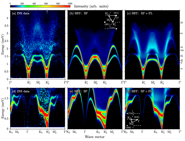
Figure 2: Comparison between the INS measurements of Ba₃CoSb₂O₉ reproduced from Ref. Macdougal et al., 2020 (left column) and the zero-temperature $I(\boldsymbol{q},\omega)$ computed with the SBT Ghioldi et al. (2018); Zhang et al. (2019, 2021) (middle and right columns). The middle column shows the mean-field result corresponding to the diagram depicted in Fig. 1(a). The right column includes contributions from both diagrams shown in Fig. 1. In all figures included in this work, the calculated $I(\boldsymbol{q},\omega)$ was multiplied by a single overall intensity scale factor to compare with the observed experimental intensity data. The brackets on the right-hand side in (c) indicate the energy cuts shown in Fig. 5. The wave-vector path in (a)-(c) is $\Gamma^{\prime}(0,1,1)$ $\rightarrow$ $\rm K_{1}^{\prime}(1/3,1/3,1)$ $\rightarrow$ $\rm M_{2}^{\prime}(0,1/2,1)$ $\rightarrow$ $\rm K_{2}^{\prime}(-1/3,2/3,1)$ $\rightarrow$ $\Gamma^{\prime}$, shown in the inset. In (d)-(f), the path is $\rm K_{2}(-1/3,2/3,0)$ $\rightarrow$ $\rm M_{2}(0,1/2,0)$ $\rightarrow$ $\rm\Gamma(0,1,0)$ $\rightarrow$ $\rm K_{2}$ $\rightarrow$ $\rm K_{2}^{\prime}(-1/3,2/3,1)$ $\rightarrow$ $\rm M_{2}^{\prime}(0,1/2,1)$ $\rightarrow$ $\Gamma^{\prime}(0,1,1)$ .

IV.1 Single-Magnon Dispersion

Figures 2(a) and 2(d) show an overview of the measured excitation spectrum of Ba₃CoSb₂O₉ along representative paths in momentum space Macdougal et al. (2020). In the notation of Ref. Macdougal et al., 2020, the wave vector labels $\Gamma$, M and K refer to the conventional high-symmetry points in the 2D hexagonal Brillouin zone (BZ), where an unprimed (primed) label indicates $l=0$ ($l=1$) and numbered subscripts refer to symmetry-related distinct points when reduced to the first BZ. The scattering intensity is strongest around the magnetic Bragg wave vectors K${}^{\prime}_{1,2}$, from which a linearly dispersing in-plane Goldstone mode emerges. The second out-of-plane mode is gapped because of the easy-plane anisotropy. A clear rotonlike minimum appears in the lower-energy mode at the M${}^{\prime}_{2}$ point, while the higher-energy mode exhibits a flattened dispersion.

Figures 2(b) and 2(e) include the $T\!=\!0$ INS cross section $I^{\rm{sp}}(\boldsymbol{q},\omega)$ obtained from the SP diagram shown in Fig. 1(a). As anticipated in the previous section, the poles of $\chi^{\rm{sp}}_{\mu\nu}(\boldsymbol{q},i\omega)$ coincide with the poles of the single-spinon propagator $\mathcal{G}^{\rm sp}$ because they arise from replacing one of the two propagators in the Feynman diagram with the contribution from the condensate $\mathcal{G}^{\rm sp}_{c}$. In addition to the single-spinon poles, $I^{\rm{sp}}(\boldsymbol{q},\omega)$ exhibits a W-shaped continuum scattering [see Fig. 2(b)] arising from the two-spinon continuum, which extends up to twice the single-spinon bandwidth: $2W_{\rm spinon}\simeq 4.32$ meV.

Figures 2(c) and 2(f) show the $T\!=\!0$ INS cross section $I(\boldsymbol{q},\omega)$ obtained from the sum of the $\rm SP$ and $\rm FL$ diagrams included in Fig. 1. The addition of the counterdiagram depicted in Fig. 1(b) changes the result at a qualitative level. As anticipated, it cancels out the residues of the single-spinon poles of $\chi^{\rm sp}_{\mu\mu}(\boldsymbol{q},\omega)$, implying that the only poles of the resulting $\chi_{\mu\mu}(\boldsymbol{q},\omega)$ are the poles of the RPA propagator [wavy line in Fig. 1(b)]. These poles correspond to the single-magnon excitations, which are the true collective modes of the system. In addition, the W-shaped two-spinon continuum, shown in Fig. 2(c), becomes more pronounced, exhibiting larger intensity and a stronger modulation as a function of energy and momentum.

The failure of NLSWT has motivated an empirical parametrization of the single-magnon dispersion with more than 10 fitting parameters Macdougal et al. (2020). Figure 3 includes a comparison between this experimentally fitted single-magnon dispersion and the single-magnon dispersion extracted from the poles of the RPA propagator. The SBT reproduces the measured magnon dispersion to a very good approximation. Remarkably, the only tuning parameter is $\alpha\!=\!0.436$, which turns out to be very close to the value $\alpha\!=\!0.5$ adopted in previous works Trumper et al. (1997); Manuel et al. (1998); Manuel and Ceccatto (1999); Ghioldi et al. (2018); Zhang et al. (2019). The comparison reveals that the overall single-magnon dispersion is very well reproduced by the SBT, which predicts a magnon velocity $c_{m}\approx 1.2J$. The only noticeable discrepancies are the small rotonlike anomalies near the $\rm M$ and $\rm K/2$ points. Returning to Fig. 2, the overall spectral weight modulation of the sharp magnons is also well reproduced over the whole Brillouin zone, except for the points that exhibit the rotonlike anomaly. This level of agreement is remarkable if we consider that NLSWT predicts a single-magnon bandwidth of 2.4 meV, which is more than 40$\%$ higher than the experimental value Ma et al. (2016). The combination of both results suggest that a free-spinon gas is a better starting point to describe the magnons of Ba₃CoSb₂O₉, which arise as two-spinon bound states in the SBT.

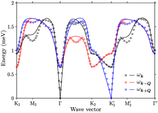
Figure 3: Comparison between the two-spinon bound state dispersion computed with SBT (full lines) and the best parametrization (open circles) of the experimentally observed magnon dispersions from Ref. Macdougal et al., 2020.

The lack of the rotonlike anomalies and the corresponding renormalization of the single-magnon spectral weight are expected shortcomings of the current level of approximation, if we consider that the diagrams shown in Fig. 1 correspond to the lowest-order approximation required to obtain the true collective modes of the theory. In other words, these diagrams do not include self-energy corrections of the single-spinon and the auxiliary field propagators. It is well known that rotonlike anomalies arise in NLSWT only after including self-energy $1/S$ corrections to the bare single-magnon propagator Starykh et al. (2006); Chernyshev and Zhitomirsky (2006); Zhitomirsky and Chernyshev (2013); Mourigal et al. (2013). In the case of the SBT, self-energy corrections to the single-spinon propagator also renormalize the single-magnon dispersion because magnons are two-spinon bound states. This renormalization is expected to shift the position of the magnon peaks relative to the onset of the two-spinon continuum. As shown in Fig. 4, the overlap between the higher-energy magnon at the $\rm M^{\prime}$ point and the two-spinon continuum leads to a strong reduction of the spectral weight, which is not observed in the experiment, where the separation between the magnon peak and the continuum is roughly 0.3 meV [see Fig. 2(a)]. Based on these observations, we conjecture that the rotonlike anomalies will arise from self-energy corrections of the single-spinon and/or single-magnon propagators.

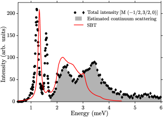
Figure 4: Comparison between INS intensity averaged over $l$ (including several zones as in Ref. Macdougal et al., 2020) and the corresponding average of the intensity $I(\boldsymbol{q},\omega)$ obtained from the two diagrams shown in Fig. 1 (solid line). A Lorentzian broadening, which accounts for the estimated experimental energy resolution, has been introduced in the calculated $I(\boldsymbol{q},\omega)$ via the replacement $\omega\to\omega+i\eta$.

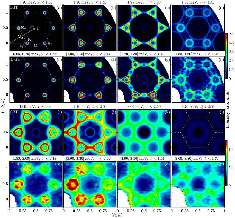
Figure 5: Intensity maps of $I({\bf q},\omega)$ [Eq. (12)] as a function of momentum in the $hk$ plane at a series of constant energies. The results have been integrated over an energy range that is indicated at the top of each panel to facilitate the comparison with INS data reproduced from Ref. Macdougal et al., 2020.

IV.2 Continuum Scattering

Another important consequence of the composite nature of the single-magnon excitations is the emergence of a highly structured two-spinon continuum, which extends up to twice the single-spinon bandwidth: $2W_{\rm spinon}\simeq 4.32$ meV. As it is clear from Figs. 2(b) and 2(c), the single-spinon bandwidth $W_{\rm spinon}\simeq 2.16$ meV is significantly larger than the single-magnon bandwidth $W_{\rm magnon}\simeq 1.7$ meV. While this difference could explain the origin of the wide energy window of continuum scattering revealed by the INS experiment, we will see below that the SBT theory is still missing spectral weight in the high-energy region at the current level of approximation.

The SBT reproduces the strong intensity modulations and the dispersion across the Brillouin zone of the low-energy part of the continuum [see Figs. 2(a) and 2(c)]. For instance, Fig. 4 shows the average over $l$ of the experimental and theoretical neutron scattering cross section at $(1/2,1/2,l)$. The theoretical ratio between the INS intensity of the continuum and the magnon peaks is approximately equal to $2.74$, which is in remarkably good agreement with the value of 2.8 that is obtained by integrating the experimental curve in Fig. 4. Importantly, this ratio is more than four times higher than the value of $\simeq 0.66$ obtained from NLSWT Kamiya et al. (2018), which clearly underestimates the relative weight of the continuum scattering. Moreover, the measured continuum scattering extends up to at least $E\simeq$ 6 meV, which is roughly equal to four times the single-magnon bandwidth Ito et al. (2017); Macdougal et al. (2020). The two diagrams included in our SBT only account for the first two low-energy stages. We attribute this discrepancy to the lack of four-spinon contributions arising from self-energy corrections to the single-spinon propagator not included in Fig. 1.

To facilitate the comparison with the the INS data Macdougal et al. (2020), Fig. 5 shows intensity maps of the measured and calculated $I({\boldsymbol{q}},\omega)$ at different energies. The comparison at energies below the top of the magnon band, shown in Figs. 5(a)-5(h), confirms the above-discussed overall agreement between experiment and theory, except for the missing rotonlike anomalies in the theoretical calculation, that explain the differences between the Figs. 5(c) and Figs. 5(g) near the M points.

Figures 5(i)-5(p) show the intensity maps arising from the continuum scattering just above the top of the one-magnon dispersion. As observed in the experiment, the continuum intensity obtained from the SBT is centered at the K points with a clear threefold symmetric pattern. The ring patterns around K, that become apparent at slightly higher energies and transform into triangular contours with corner touchings at the M points, are also reproduced by the SBT. However, the ring patterns of the theoretical calculation are rotated by an angle $\pi/3$ relative to the ring patterns of the experimental data [see Figs. 5(i) and 5(m)]. Once again, we attribute this difference to the absence of the rotonlike anomaly in the theoretical calculation. As shown in Fig. 4, the neutron scattering intensity of the measured upper magnon peak near the M points is significantly larger than the calculated intensity. It is then expected that self-energy corrections to the single-spinon propagator, which account for the rotonlike anomaly, should transfer spectral weight from the low-energy continuum (around $E\simeq 2$ meV) to the upper magnon peak. The excess of continuum spectral weight near the M points at the current level of approximation explains the $\pi/3$ rotation of the ring patterns and the “bridges” that connect adjacent rings in Fig. 5(j), which do not have a counterpart in the experimental data shown in Figs. 5(n). Finally, as it is clear from the comparison between Fig. 5(l) and 5(p), the relatively large spectral weight of the measured continuum scattering in the high-energy interval ranging from 3.6 to 3.8 meV is not reproduced by the SBT at the current level of approximation (see Fig. 4).

V Discussion

Our detailed comparison between the SBT and the INS cross section of Ba₃CoSb₂O₉ reveals, for the first time, that a low-order expansion in the control parameter ($1/N$) provides an adequate framework to describe the magnetic excitations of quasi-$2\rm D$ TLHA. In contrast, semiclassical treatments overestimate the single-magnon bandwidth by approximately 40% and they cannot account for the large intensity and modulation of the observed continuum scattering Ma et al. (2016); Ito et al. (2017). Thus, we attribute the failure of the large-$S$ expansion to the proximity of Ba₃CoSb₂O₉ to a QCP that signals the onset of a QSL. Since the elementary excitations of the QSL phase are quasifree single spinons, a free-spinon gas becomes a better starting point than a free-magnon gas near the QCP. Magnons are then recovered on the magnetically ordered side as two-spinon bound states (poles of the RPA propagator) induced by fluctuations of the emergent gauge fields. Within the SBT, the gapped $\mathbb{Z}_{2}$ QSL state proposed by Sachdev Sachdev (1992) is the only liquid which can be continuously connected with a $120^{\circ}$ Néel ordered state Wang and Vishwanath (2006), as it does not break any symmetries and has its lowest energy modes at the $\rm K$ points. The resulting quantum critical point is expected to have a dynamically generated $O(4)$ symmetry Azaria et al. (1990); Chubukov et al. (1994).

Alternative parton theories with fermionic matter fields lead to a different spin liquid state on the other side of the QCP, such as a gapless U(1) spin liquid Dupuis et al. (2019); Hu et al. (2019). However, while existing attempts to reproduce the unusual excitation spectrum of the ordered phase using fermionic partons seem to account for the rotonlike anomaly, the results have not been compared against the available experimental data Zhang and Li (2020); Ferrari and Becca (2019).

Extended continua has also been observed in ladder Lake et al. (1978) and spatially anisotropic triangular Kohno et al. (2007) systems -experimentally realized in CaCu₂O₃ and Cs₂CuCl₄ compounds Lake et al. (1978); Kohno et al. (2007), respectively. These continua have been attributed to 1D spinons which are confined by the interchain interactions. This is in sharp contrast to the 2D character of the spinons invoked in this work, which are the building blocks of the SBT and interact via emergent gauge fields consisting of the Lagrange multiplier and phases of the bond fields $W_{ij}^{X}$.

Our results have implications for other quantum magnets that are described by a similar model. For instance, the delafossite triangular lattice materials, such as CsYbSe₂ Xie et al. (2021) and NaYbSe₂, could lie even closer to the quantum melting point, while the triangular layers of Ba₂CoTeO₆ Kojima et al. (2022) exhibit an INS spectrum that is remarkably similar to the one of Ba₃CoSb₂O₉. A very recent tensor network study of the triangular XXZ model Chi et al. (2022) reinforces the validity of this model to quantitatively describe the magnetic excitations of Ba₃CoSb₂O₉. Recently, we also became aware of Ref. Syromyatnikov, 2022, which attempts to solve the same problem using a different approach.

VI Acknowledgments

We thank Radu Coldea for a critical reading of our manuscript and for providing detailed explanations of the data presented in Ref. Macdougal et al., 2020. We also acknowledge useful discussions with D. A. Tennant, A. Scheie, C. J. Gazza, O. Starykh, Alexander Chernyshev, and M. Mourigal. The work by C.D.B. was supported by the U.S. Department of Energy, Office of Science, Basic Energy Sciences, Materials Sciences and Engineering Division under Award No. DE-SC-0018660. Y.K. acknowledges the support by the NSFC (Grants No. 12074246 and No. U2032213) and MOST (Grants No. 2016YFA0300500 and No. 2016YFA0300501) research programs. E.A.G., L.O.M and A.E.T. were supported by CONICET under Grant PIP No. 3220.

References

- Knolle and Moessner (2019) J. Knolle and R. Moessner, Annual Review of Condensed Matter Physics 10, 451 (2019).
- Broholm et al. (2020) C. Broholm, R. J. Cava, S. A. Kivelson, D. G. Nocera, M. R. Norman, and T. Senthil, Science 367 (2020), 10.1126/science.aay0668.
- Savary and Balents (2016) L. Savary and L. Balents, Reports on Progress in Physics 80, 016502 (2016).
- Kitaev (2003) A. Kitaev, Annals of Physics 303, 2 (2003).
- Tokura et al. (2017) Y. Tokura, M. Kawasaki, and N. Nagaosa, Nature Physics 13, 1056 (2017).
- Anderson (1973) P. Anderson, Materials Research Bulletin 8, 153 (1973).
- Capriotti et al. (1999) L. Capriotti, A. E. Trumper, and S. Sorella, Phys. Rev. Lett. 82, 3899 (1999).
- White and Chernyshev (2007) S. R. White and A. L. Chernyshev, Phys. Rev. Lett. 99, 127004 (2007).
- Hu et al. (2015) W.-J. Hu, S.-S. Gong, W. Zhu, and D. N. Sheng, Phys. Rev. B 92, 140403 (2015).
- Iqbal et al. (2016) Y. Iqbal, W.-J. Hu, R. Thomale, D. Poilblanc, and F. Becca, Phys. Rev. B 93, 144411 (2016).
- Saadatmand and McCulloch (2016) S. N. Saadatmand and I. P. McCulloch, Phys. Rev. B 94, 121111 (2016).
- Wietek and Läuchli (2017) A. Wietek and A. M. Läuchli, Phys. Rev. B 95, 035141 (2017).
- Gong et al. (2017) S.-S. Gong, W. Zhu, J.-X. Zhu, D. N. Sheng, and K. Yang, Phys. Rev. B 96, 075116 (2017).
- Hu et al. (2019) S. Hu, W. Zhu, S. Eggert, and Y.-C. He, Phys. Rev. Lett. 123, 207203 (2019).
- Zhu and White (2015) Z. Zhu and S. R. White, Phys. Rev. B 92, 041105 (2015).
- Zhu et al. (2018) Z. Zhu, P. A. Maksimov, S. R. White, and A. L. Chernyshev, Phys. Rev. Lett. 120, 207203 (2018).
- Manuel and Ceccatto (1999) L. O. Manuel and H. A. Ceccatto, Phys. Rev. B 60, 9489 (1999).
- Mishmash et al. (2013) R. V. Mishmash, J. R. Garrison, S. Bieri, and C. Xu, Phys. Rev. Lett. 111, 157203 (2013).
- Kaneko et al. (2014) R. Kaneko, S. Morita, and M. Imada, Journal of the Physical Society of Japan 83, 093707 (2014), https://doi.org/10.7566/JPSJ.83.093707 .
- Li et al. (2015) P. H. Y. Li, R. F. Bishop, and C. E. Campbell, Phys. Rev. B 91, 014426 (2015).
- Arovas and Auerbach (1988) D. P. Arovas and A. Auerbach, Phys. Rev. B 38, 316 (1988).
- Sachdev and Read (1991) S. Sachdev and N. Read, International Journal of Modern Physics B 05, 219 (1991).
- Read and Sachdev (1991) N. Read and S. Sachdev, Phys. Rev. Lett. 66, 1773 (1991).
- Chubukov et al. (1994) A. V. Chubukov, S. Sachdev, and T. Senthil, Nuclear Physics B 426, 601 (1994).
- Chubukov and Starykh (1996) A. V. Chubukov and O. A. Starykh, Phys. Rev. B 53, R14729 (1996).
- Auerbach (1994) A. Auerbach, Interacting electrons and quantum magnetism (Springer-Verlag, New York, 1994).
- Ghioldi et al. (2018) E. A. Ghioldi, M. G. Gonzalez, S.-S. Zhang, Y. Kamiya, L. O. Manuel, A. E. Trumper, and C. D. Batista, Phys. Rev. B 98, 184403 (2018).
- Zhang et al. (2019) S.-S. Zhang, E. A. Ghioldi, Y. Kamiya, L. O. Manuel, A. E. Trumper, and C. D. Batista, Phys. Rev. B 100, 104431 (2019).
- Zhang et al. (2021) S.-S. Zhang, E. A. Ghioldi, L. O. Manuel, A. E. Trumper, and C. D. Batista, “Schwinger boson theory of ordered magnets,” (2021), arXiv:2109.03964 [cond-mat.str-el] .
- Macdougal et al. (2020) D. Macdougal, S. Williams, D. Prabhakaran, R. I. Bewley, D. J. Voneshen, and R. Coldea, Phys. Rev. B 102, 064421 (2020).
- Zhou et al. (2012) H. D. Zhou, C. Xu, A. M. Hallas, H. J. Silverstein, C. R. Wiebe, I. Umegaki, J. Q. Yan, T. P. Murphy, J.-H. Park, Y. Qiu, J. R. D. Copley, J. S. Gardner, and Y. Takano, Phys. Rev. Lett. 109, 267206 (2012).
- Ito et al. (2017) S. Ito, N. Kurita, H. Tanaka, S. Ohira-Kawamura, K. Nakajima, S. Itoh, K. Kuwahara, and K. Kakurai, Nature Communications 8, 235 (2017).
- Ma et al. (2016) J. Ma, Y. Kamiya, T. Hong, H. B. Cao, G. Ehlers, W. Tian, C. D. Batista, Z. L. Dun, H. D. Zhou, and M. Matsuda, Phys. Rev. Lett. 116, 087201 (2016).
- Kamiya et al. (2018) Y. Kamiya, L. Ge, T. Hong, Y. Qiu, D. L. Quintero-Castro, Z. Lu, H. B. Cao, M. Matsuda, E. S. Choi, C. D. Batista, M. Mourigal, H. D. Zhou, and J. Ma, Nature Communications 9, 2666 (2018).
- Scheie et al. (2021) A. O. Scheie, E. A. Ghioldi, J. Xing, J. A. M. Paddison, N. E. Sherman, M. Dupont, D. Abernathy, D. M. Pajerowski, S.-S. Zhang, L. O. Manuel, A. E. Trumper, C. D. Pemmaraju, A. S. Sefat, D. S. Parker, T. P. Devereaux, J. E. Moore, C. D. Batista, and D. A. Tennant, “Witnessing quantum criticality and entanglement in the triangular antiferromagnet kybse2,” (2021), arXiv:2109.11527 [cond-mat.str-el] .
- Doi et al. (2004) Y. Doi, Y. Hinatsu, and K. Ohoyama, J. Phys.: Condens. Matter 16, 8923 (2004).
- Susuki et al. (2013) T. Susuki, N. Kurita, T. Tanaka, H. Nojiri, A. Matsuo, K. Kindo, and H. Tanaka, Phys. Rev. Lett. 110, 267201 (2013).
- Koutroulakis et al. (2015) G. Koutroulakis, T. Zhou, Y. Kamiya, J. D. Thompson, H. D. Zhou, C. D. Batista, and S. E. Brown, Phys. Rev. B 91, 024410 (2015).
- Note (1) The high-symmetry structure of this material forbids Dzyaloshinskii-Moriya interactions between Co2+ ions in the same plane or relatively displaced along the -axis.
- Chubukov and Golosov (1991) A. V. Chubukov and D. I. Golosov, Journal of Physics: Condensed Matter 3, 69 (1991).
- Shirata et al. (2012) Y. Shirata, H. Tanaka, A. Matsuo, and K. Kindo, Phys. Rev. Lett. 108, 057205 (2012).
- Quirion et al. (2015) G. Quirion, M. Lapointe-Major, M. Poirier, J. A. Quilliam, Z. L. Dun, and H. D. Zhou, Phys. Rev. B 92, 014414 (2015).
- Sera et al. (2016) A. Sera, Y. Kousaka, J. Akimitsu, M. Sera, T. Kawamata, Y. Koike, and K. Inoue, Phys. Rev. B 94, 214408 (2016).
- Alicea et al. (2009) J. Alicea, A. V. Chubukov, and O. A. Starykh, Phys. Rev. Lett. 102, 137201 (2009).
- Ghioldi et al. (2015) E. A. Ghioldi, A. Mezio, L. O. Manuel, R. R. P. Singh, J. Oitmaa, and A. E. Trumper, Phys. Rev. B 91, 134423 (2015).
- Auerbach and Arovas (1988) A. Auerbach and D. P. Arovas, Phys. Rev. Lett. 61, 617 (1988).
- Fåk et al. (2012) B. Fåk, E. Kermarrec, L. Messio, B. Bernu, C. Lhuillier, F. Bert, P. Mendels, B. Koteswararao, F. Bouquet, J. Ollivier, A. D. Hillier, A. Amato, R. H. Colman, and A. S. Wills, Phys. Rev. Lett. 109, 037208 (2012).
- Samajdar et al. (2019) R. Samajdar, S. Chatterjee, S. Sachdev, and M. S. Scheurer, Phys. Rev. B 99, 165126 (2019).
- Chandra et al. (1990) P. Chandra, P. Coleman, and A. I. Larkin, Journal of Physics: Condensed Matter 2, 7933 (1990).
- Trumper et al. (1997) A. E. Trumper, L. O. Manuel, C. J. Gazza, and H. A. Ceccatto, Phys. Rev. Lett. 78, 2216 (1997).
- Manuel et al. (1998) L. O. Manuel, A. E. Trumper, and H. A. Ceccatto, Phys. Rev. B 57, 8348 (1998).
- Starykh et al. (2006) O. A. Starykh, A. V. Chubukov, and A. G. Abanov, Phys. Rev. B 74, 180403 (2006).
- Chernyshev and Zhitomirsky (2006) A. L. Chernyshev and M. E. Zhitomirsky, Phys. Rev. Lett. 97, 207202 (2006).
- Zhitomirsky and Chernyshev (2013) M. E. Zhitomirsky and A. L. Chernyshev, Rev. Mod. Phys. 85, 219 (2013).
- Mourigal et al. (2013) M. Mourigal, W. T. Fuhrman, A. L. Chernyshev, and M. E. Zhitomirsky, Phys. Rev. B 88, 094407 (2013).
- Sachdev (1992) S. Sachdev, Phys. Rev. B 45, 12377 (1992).
- Wang and Vishwanath (2006) F. Wang and A. Vishwanath, Phys. Rev. B 74, 174423 (2006).
- Azaria et al. (1990) P. Azaria, B. Delamotte, and T. Jolicoeur, Phys. Rev. Lett. 64, 3175 (1990).
- Dupuis et al. (2019) E. Dupuis, M. B. Paranjape, and W. Witczak-Krempa, Phys. Rev. B 100, 094443 (2019).
- Zhang and Li (2020) C. Zhang and T. Li, Phys. Rev. B 102, 075108 (2020).
- Ferrari and Becca (2019) F. Ferrari and F. Becca, Phys. Rev. X 9, 031026 (2019).
- Lake et al. (1978) B. Lake, A. M. Tsvelik, S. Notbohm, D. Alan Tennant, T. G. Perring, M. Reehuis, C. Sekar, G. Krabbes, and B. Büchner, Nature Physics 6, 327 (1978).
- Kohno et al. (2007) M. Kohno, O. A. Starykh, and L. Balents, Nat. Phys 3, 790 (2007).
- Xie et al. (2021) T. Xie, J. Xing, S. Nikitin, S. Nishimoto, M. Brando, P. Khanenko, J. Sichelschmidt, L. Sanjeewa, A. S. Sefat, and A. Podlesnyak, arXiv preprint arXiv:2106.12451 (2021).
- Kojima et al. (2022) Y. Kojima, N. Kurita, H. Tanaka, and K. Nakajima, Phys. Rev. B 105, L020408 (2022).
- Chi et al. (2022) R.-Z. Chi, Y. Liu, Y. Wan, H.-J. Liao, and T. Xiang, “Spin excitation spectra of the spin-1/2 triangular heisenberg antiferromagnets from tensor networks,” (2022), arXiv:2201.12121 [cond-mat.str-el] .
- Syromyatnikov (2022) A. V. Syromyatnikov, “Novel elementary excitations in spin-1/2 antiferromagnets on the triangular lattice,” (2022), arXiv:2107.00256 [cond-mat.str-el] .