End-to-End Quality-of-Service Assurance with Autonomous Systems: 5G/6G Case Study

Abstract

Providing differentiated services to meet the unique requirements of different use cases is a major goal of the fifth generation (5G) telecommunication networks and will be even more critical for future 6G systems. Fulfilling this goal requires the ability to assure quality of service (QoS) end to end (E2E), which remains a challenge. A key factor that makes E2E QoS assurance difficult in a telecommunication system is that access networks (ANs) and core networks (CNs) manage their resources autonomously. So far, few results have been available that can ensure E2E QoS over autonomously managed ANs and CNs. Existing techniques rely predominately on each subsystem to meet static local QoS budgets with no recourse in case any subsystem fails to meet its local budgets and, hence will have difficulty delivering E2E assurance. Moreover, most existing distributed optimization techniques that can be applied to assure E2E QoS over autonomous subsystems require the subsystems to exchange sensitive information such as their local decision variables. This paper presents a novel framework and a distributed algorithm that can enable ANs and CNs to autonomously “cooperate” with each other to dynamically negotiate their local QoS budgets and to collectively meet E2E QoS goals by sharing only their estimates of the global constraint functions, without disclosing their local decision variables. We prove that this new distributed algorithm converges to an optimal solution almost surely, and also present numerical results to demonstrate that the convergence occurs quickly even with measurement noise.

I Introduction

A major goal of the fifth generation (5G) telecommunication networks is to provide differentiated (or even optimized) services to meet different use cases’ unique requirements, e.g., on performance, availability, and security [1]. The ability to provide such differentiated support is a prerequisite for many IoT (Internet of Things) applications such as automated manufacturing, vehicle-to-vehicle communications, remote operation (teleoperation) of ground vehicles and drones, and telesurgery. It represents a fundamental advancement over the previous generations of networks that had focused on providing one-size-fits-all network connectivity for all applications.

To enable differentiated services, 5G shifted from a communication-centric architecture to a service-centric architecture that separated network and service control functions from the physical infrastructure, further modularized these functions, and defined their interactions in terms of providing and consuming services. This service-centric architecture enables network slicing that creates end-to-end (E2E) logical networks (network slices) dedicated for specific services, forming a foundation for delivering differentiated services. Current 5G specifications further describe a framework and its enabling protocols for collecting network performance data required to support service assurance [3, 4, 5, 6, 7].

Despite recent advances, fundamental challenges remain to be addressed before the promise of differentiated services can be fully realized in 5G and future generations of telecommunication networks [19]. One such challenge is to assure E2E quality of service (QoS). Such assurance is essential to, for example, many delay-sensitive applications [24, 25] and will be more critical for future 6G systems that will support more use cases and more stringent requirements [15, 19].

A key factor that makes E2E service assurance difficult in telecommunication networks is the fact that access networks (ANs) and core networks (CNs) manage their resources autonomously. While such autonomous management simplifies the tasks of designing, operating, and evolving a large system, limited coordination among ANs and CNs on resource management also leaves E2E service assurance more challenging [20].

To achieve E2E QoS assurance over autonomously managed ANs and CNs, current 5G specifications decompose the E2E Key Performance Indicator (KPI) targets (e.g., packet delay, packet drop ratio) into KPI budgets for each CN and AN, and rely on each of them to autonomously manage its resources to satisfy its allocated KPI budgets. For example, 5G specifications decompose the E2E Packet Delay Budgets (PDBs) into CN PDBs and AN PDBs, with the CN PDBs for standardized QoS flows predefined in the specifications and to be statically configured in each CN [2]. A network operator will then need to determine the AN PDBs for each AN, which is done statically today.

Static KPI budget allocations cannot effectively respond to dynamic network conditions or account for the varying characteristics of different networks (e.g., different network capabilities, capacities, and supported services). Also, since an AN or CN may violate its KPI budgets due to random events such as network congestion, network operators will need ways to ensure that such violations will not lead to intolerable violations of E2E KPI requirements.

Recognizing the limitations of static KPI budget allocations, 5G permits non-standard QoS flows to support dynamic PDBs and allows the dynamic PDBs to be signaled between ANs and CNs. However, current 5G specifications do not prescribe how dynamic PDBs for each AN or CN should be determined or enforced, and how E2E PDB requirements can be assured in case any autonomous network along an E2E path violates its allocated PDB budgets.

The past few years have also seen growing efforts in developing resource allocation mechanisms for assuring E2E QoS for 5G and beyond systems. Here, we summarize only the most closely related studies that focused on E2E QoS rather than QoS for RANs or CNs alone. We emphasize that this is not meant to be an exhaustive list. In [14], the 5G QoS architecture is extended to incorporate the Framework for Abstraction and Control of Traffic Engineered Networks (ACTN), which was developed by the IETF (IETF RFC 8453) to manage large multi-domain networks. This extended architecture calls for the resource controllers in different technology or administrative domains (e.g., ANs and CNs) to be orchestrated by a Multi-Domain Service Coordinator function to achieve E2E service assurance. But, it does not describe how such orchestration can be accomplished. In [22], a high-level architecture for 5G service assurance is described. It focuses on monitoring E2E KPIs rather than providing mechanisms for achieving E2E service assurance. A dynamic resource slicing method aimed at E2E service assurance is proposed in [23], and it treats resource slicing in the radio ANs and the CN independently. A technique that combines user device QoS provisioning with network QoS provisioning is proposed in [8]. It treats QoS provisioning in ANs and CNs as independent tasks and relies on an unrealistic assumption that the KPI budgets for each network node are fixed and known. In [11], path configuration methods are proposed for ensuring E2E QoS in Software-Defined Networks (SDNs). SDNs are expected to be widely used in 5G systems. But, the path configuration methods in [11] require centralized provisioning and control of E2E network paths, which is impractical in telecommunication systems where ANs and CNs are expected to continue to be managed separately.

In order to assure E2E service quality while allowing the ANs and the CNs to control their resources independently, these autonomous networks should be able to coordinate with each other to meet E2E KPI requirements. To this end, we propose an optimization-based framework in which the E2E KPI requirements are captured by global constraints. Based on this framework, we design a new distributed algorithm; existing distributed optimization algorithms require the subsystems to maintain and exchange their local decision variables with each other. This can result in heavy signaling overheads, increase technology inter-dependency among ANs and CNs, or reveal how different subsystems manage their internal resources, and thus are impractical or undesirable in telecommunication systems [9, 12, 21].

In contrast, our algorithm only needs the subsystems to exchange their estimates of the global constraint functions. When the subsystems update their local decision variables using the proposed algorithm, they converge to an optimal point with probability 1. We present numerical results to demonstrate that the proposed algorithm quickly reduces the cost of the system to near the optimal value even with measurement noise. Finally, we illustrate that each optimal point gives rise to a stationary state Nash equilibrium of an associated state-based potential game.

Notation: We denote set of nonnegative integers by ${\rm I\kern-2.5ptN}$. Unless stated otherwise, all vectors are column vectors and $\left|\left|\cdot\right|\right|_{2}$ denotes the $\ell_{2}$ norm. Given a vector ${\bf x}$, we denote the $k$th element by $x_{k}$. The vector of zeros (resp. ones) of appropriate dimension is denoted by $\mathbf{0}$ (resp. $\mathbf{1}$). Given a closed convex set ${\cal S}$ and a vector ${\bf x}$, $P_{{\cal S}}({\bf x})$ denotes the Euclidean projection of ${\bf x}$ onto ${\cal S}$.

II Proposed Optimization Framework

In the rest of the paper, we refer to an AN or a CN as an agent, and let ${\cal A}$ be the set of $N$ agents. The problem of ensuring E2E QoS over autonomously managed networks can be formulated as a distributed optimization problem with both local and global constraints. Let $\mathbf{y}_{i}$ be the local decision variables of agent $i\in{\cal A}$, which are used by agent $i$ to manage its network resources. The local constraints of agent $i$ restrict $\mathbf{y}_{i}$ independently of the decision variables chosen by other agents. We call the set of ${\bf y}_{i}$ that satisfies agent $i$’s local constraints its local constraint set and denote it by ${\cal G}_{i}$. Let ${\bf y}:=({\bf y}_{i}:i\in{\cal A})$ be the vector comprising the decision variables of all agents. The set of ${\bf y}$ that satisfies the local constraints of all agents is denoted by ${\cal G}:=\prod_{i\in{\cal A}}{\cal G}_{i}$.

We capture the E2E QoS guarantees, which the agents must meet collectively, using $K$ global constraint functions $g_{1},\ldots,g_{K}$. The global constraints depend on the decision variables of more than one agent and, hence, require their coordination.

If (i) the local objective functions of individual agents, (ii) local constraint sets ${\cal G}_{i}$, $i\in{\cal A}$, and (iii) global constraint functions $g_{1},\ldots,g_{K}$ are known, we can formulate the problem of optimizing the overall network performance subject to the E2E QoS requirements as a constrained optimization problem of the form given below, where (a) the objective function is separable, and (b) global (inequality) constraints couple the decision variables of agents:

$$\min_{{\bf y}\in{\cal G}} \sum_{i\in{\cal A}}\phi_{i}({\bf y}_{i})$$ (1a)

s.t. $$\mathbf{g}(\mathbf{y}):=\sum_{i\in\mathcal{A}}\mathbf{g}_{i}(\mathbf{y}_{i})\leq\mathbf{0},$$ (1b)

where $\phi_{i}$ denotes the local objective function that agent $i$ aims to minimize using its decision variables $\mathbf{y}_{i}$. Here, $\mathbf{g}:=(g_{1},\ldots,g_{K})$ is the vector function consisting of $K$ global constraint functions. In our setting, each agent $i$ knows ${\bf g}_{i}$, which represents its contributions to global constraint functions, but not $\mathbf{g}_{j}$, $j\in{\cal A}\setminus\{i\}$.

II-A Example: End-to-end Delay Constraints

Consider a network consisting of $N$ domains or autonomous systems, which are the agents in our framework, and denote the set of agents by ${\cal A}$. Suppose that the network provides $n_{S}$ different service classes and ${\cal S}$ is the set of service classes. Let ${\cal F}$ be the set of $n_{F}$ flows that need to be supported. Each flow $f\in{\cal F}$ is of service class $s_{f}\in{\cal S}$. Thus, the set ${\cal F}$ can be partitioned into $\{{\cal F}^{s}:s\in{\cal S}\}$, where ${\cal F}^{s}$ is the set of service class $s$ flows in ${\cal F}$ with $n^{s}:=|{\cal F}^{s}|$, $s\in{\cal S}$. Each flow $f$ traverses a subset of agents in ${\cal A}_{f}$. We use an $n^{s}\times N$ matrix ${\bf R}^{s}=[R^{s}_{f,a}:f\in{\cal F}^{s},a\in{\cal A}]$ to describe the routes taken by the flows of service class $s$, where $R^{s}_{f,a}=1$ if flow $f$ traverses agent $a$, and $R^{s}_{f,a}=0$ otherwise.

Problem for individual agents

Let ${\cal N}^{a}$ be the set of egress/ingress nodes in agent $a$ and $m^{a}:=|{\cal N}^{a}|$. An agent $a$’s flow $b$ refers to a triple $(s,p_{i},p_{e})\in{\cal S}\times{\cal N}^{a}\times{\cal N}^{a}$ with the understanding that it carries service class $s$ traffic that enters and leaves agent $a$ at $p_{i}$ (ingress point) and $p_{e}$ (egress point), respectively. We denote the set of flows of service class $s$ in agent $a$ by $\tilde{{\cal F}}^{a}_{s}$, and let $\tilde{{\cal F}}^{a}:=\cup_{s\ \in{\cal A}}\tilde{{\cal F}}^{a}_{s}$.

For each agent $a\in{\cal A}$, there is a fixed traffic tensor that describes the amount of traffic that needs to be transported for each ingress-egress pair and each service class. We denote this traffic tensor by ${\bf T}^{a}$, which is an $n_{s}\times m^{a}\times m^{a}$ tensor; the element $T^{a}_{s,p_{i},p_{e}}$ denotes the demand of flow $b=(s,p_{i},p_{e})$, i.e., it is the amount of traffic belonging to service class $s\in{\cal S}$, which needs to be transported from ingress node $p_{i}\in{\cal N}^{a}$ to egress node $p_{e}\in{\cal N}^{a}$. We use $I(b)$ and $E(b)$ to denote the ingress and egress node, respectively, of flow $b$.

Let ${\cal L}^{a}$ be the set of (directed) links in agent $a$. Each link $\ell\in{\cal L}^{a}$ has a finite capacity $c^{a}_{\ell}$, and ${\bf c}^{a}:=(c^{a}_{\ell}:\ell\in{\cal L}^{a})$. Each flow $b\in\tilde{{\cal F}}^{a}$ is supported by a set of routes in ${\cal R}^{a}_{b}$ connecting $I(b)$ to $E(b)$, and a route $r\in{\cal R}^{a}_{b}$ utilizes a subset of links in agent $a$, which we denote by ${\cal L}^{a}(r)$ with a little abuse of notation. For each $s\in{\cal S}$, we define ${\cal P}^{a}_{s}:=\cup_{b\in\tilde{{\cal F}}^{a}_{s}}{\cal R}^{a}_{b}$ and a routing matrix ${\bf R}^{a}_{s}$, which is a $|{\cal P}^{a}_{s}|\times|{\cal L}^{a}|$ matrix; the element $R^{a}_{r,\ell}=1$ if $\ell\in{\cal L}^{a}(r)$ and $R^{a}_{r,\ell}=0$ otherwise.

The variable $x^{a}_{b,r},r\in{\cal R}^{a}_{b}$ for some flow $b\in\tilde{{\cal F}}^{a}$, denotes the amount of flow $b$ traffic traversing route $r$. Define ${\bf x}^{a}=(x^{a}_{b,r}:b\in\tilde{{\cal F}}^{a}\mbox{ and }r\in{\cal R}^{a}_{b})$ to be the local decision variables of agent $a$. These local decision variables must be nonnegative and support the given traffic tensor: for every $b\in{\cal F}^{a}$,

$$\textstyle x^{a}_{b,r}\geq 0\mbox{ for all }r\in{\cal R}^{a}_{b}\ \mbox{ and }\ \sum_{r\in{\cal R}^{a}_{b}}x^{a}_{b,r}=T^{a}_{b}.$$

We use ${\cal G}_{a}$ to denote the set of agent $a$’s decision variables that satisfy these conditions.

The goal of agent $a$ is to minimize its own local cost given by $C^{a}({\bf x}^{a})$. This local cost $C^{a}({\bf x}^{a})$ can be, for example, the (weighted) average delay experienced by the traffic traversing agent $a$ or the costs associated with packet losses suffered in its network. Oftentimes, this cost includes a summable cost, i.e., the sum of the costs of individual links, which can be written as $\textstyle\sum_{s\in{\cal S}}\left(\textstyle\sum_{\ell\in{\cal L}^{a}}c_{s,\ell}({\bf x}^{a})\right)$, where $c_{s,\ell}({\bf x}^{a})$ is the cost of class $s$ traffic on link $\ell$ as a function of ${\bf x}^{a}$.

E2E delay requirements

The traffic of service class $s$ cannot tolerate (average) E2E delays larger than $d^{*}(s)$. We handle these E2E delay constraints using the following global constraints: suppose that, given local decision variables ${\bf x}^{a}$ of agent $a$, the delay experienced by service class $s$ traffic on link $\ell$ is given by $D^{a}_{s,\ell}({\bf x}^{a})$. Then, the delays experienced by flows of service class $s$ through agent $a$ are given by

$${\bf R}^{a}_{s}{\bf D}^{a}_{s}({\bf x}^{a}),$$

where ${\bf D}^{a}_{s}({\bf x}^{a}):=(D^{a}_{s,\ell}({\bf x}^{a}):\ell\in{\cal L}^{a})$. In general, it is reasonable to assume that $D^{a}_{s,\ell}({\bf x}^{a})$ is a convex function of ${\bf x}^{a}$. We define

$$g_{a,s}({\bf x}^{a}):=\max({\bf R}^{a}_{s}{\bf D}^{a}_{s}({\bf x}^{a})),\quad s\in{\cal S},$$

to be the maximum delay experienced by service class $s$ traffic in agent $a$’s network.

Let ${\bf x}:=({\bf x}^{a}:a\in{\cal A})$ and ${\cal G}:=\prod_{a\in{\cal A}}{\cal G}_{a}$. The problem of minimizing the total cost of all agents can be set up as the following constrained optimization problem:

$$\min_{{\bf x}\in{\cal G}} \sum_{a\in{\cal A}}C^{a}({\bf x}^{a})$$ (2a)

s.t. $$\sum_{a\in\mathcal{A}}R^{s}_{f,a}g_{a,s}({\bf x}^{a})\leq d^{*}(s),\ s\in{\cal S}\mbox{ and }f\in\mathcal{F}^{s}$$ (2b)

It is evident that the above problem in (2) is of the form in (1). Note that the decisions by the agents are coupled only via the constraints in (2b), while the objective function is separable.

III Distributed Optimization Algorithm with Noisy Measurements

It is clear from the discussion and the example in the previous section that, in order for the agents to optimize the overall network performance with global constraints, we need a new distributed optimization framework that will allow the agents to cooperate with each other to satisfy the global constraints without incurring prohibitive overheads for information exchange. Furthermore, in order to allow different agents to use different networking technologies, equipment, and equipment vendors, it will be important to eliminate or minimize the need for the agents to exchange sensitive information that may reveal how they manage their networks.

III-A Penalty Method with Noisy Measurements

One popular approach to solving a constrained optimization problem is a penalty method, which adds a penalty function to the objective function. The penalty increases with the level of violations of constraints. Although a general penalty function can be used in our problem, we assume a specific penalty function to simplify our exposition: consider the following approximated problem with a penalty function:

$$\min_{{\bf y}\in{\cal G}}\quad\sum_{i\in{\cal A}}\phi_{i}({\bf y}_{i})+\frac{\mu}{2N}\sum_{k\in{\cal K}_{G}}\big{(}[g_{k}(\mathbf{y})]_{+}\big{)}^{2}=:\Phi(\mathbf{y}),$$ (3)

where $\mu>0$ is a penalty parameter, ${\cal K}_{G}$ is the set of $K$ global constraints, $\phi_{i}$ is the (local) objective function of agent $i$ (introduced in (1)), and $[\cdot]_{+}:=\max(0,\cdot)$. The original problem in (1) is recovered by letting $\mu\to\infty$. The function $\Phi$ is convex on ${\cal G}$ provided that $\phi_{i}$ and $g_{i,k}$, $i\in{\cal A}$ and $k\in{\cal K}_{G}$, are convex.

Unfortunately, the usual gradient projection method does not lead to a distributed algorithm for our problem because the penalty function and its gradient are coupled. Also, in many problems of practical interest, (a) the analytic expression of $\phi_{i}$ and its gradient are unknown to agent $i$ and (b) only noisy measurements are available to estimate them. For instance, in the example discussed in the previous section, an agent needs to estimate its local costs from network measurements (e.g., packet loss rates), which contain measurement noise.

In order to deal with the issues of (i) noisy estimates of local costs and (ii) global constraints that couple the decision variables of agents, we propose a new distributed optimization algorithm that requires each agent $i$ to keep an estimate $\mathbf{e}_{i}(t)$ of the constraint functions ${\bf g}(\mathbf{y}(t))$. These estimates are used to approximate the gradient of the penalty function and are updated using a consensus-type algorithm.

Update rule for decision variables

Consider the following iterative update rule, which is used by each agent to update its local decision variables: for every agent $i\in{\cal A}$ and $t\in{\rm I\kern-2.5ptN}$,

$$\mathbf{y}_{i}(t+1) = P_{{\cal G}_{i}}\big{(}\mathbf{y}_{i}(t)+\gamma_{t}{\bf U}_{i}(t)\big{)},$$ (4)

where ${\bf U}_{i}(t)$ are random vectors, and $\gamma_{t}$ is a step size at iteration $t$. The initial value $\mathbf{y}_{i}(0)$ is chosen arbitrarily in $\mathcal{G}_{i}$. The random vector can be decomposed as follows:

$${\bf U}_{i}(t)=-\nabla\phi_{i}(\mathbf{y}_{i}(t))\!-\!\frac{\mu}{N}\sum_{k\in{\cal K}_{G}}\!\!\nabla g_{i,k}(\mathbf{y}_{i}(t))[g_{k}(\mathbf{y}(t))]_{+}$$ (5)

$$+\mu\sum_{k\in{\cal K}_{G}}\!\!\nabla g_{i,k}(\mathbf{y}_{i}(t))\Big{(}\frac{1}{N}[g_{k}(\mathbf{y}(t))]_{+}\!-\![e_{i,k}(t)]_{+}\Big{)}\!+\!{\bf V}_{i}(t)$$

$$=-\nabla\phi_{i}(\mathbf{y}_{i}(t))\!-\!\mu\sum_{k\in{\cal K}_{G}}\!\!\nabla g_{i,k}(\mathbf{y}_{i}(t))[e_{i,k}(t)]_{+}\!+\!{\bf V}_{i}(t).$$

The first and second terms on the right-hand side (RHS) in (5) are the gradient of the local objective function $\phi_{i}$ and the penalty function associated with global constraints, respectively. The third term models the difference between the correct gradient of the penalty function and the estimated gradient on the basis of agent $i$’s estimates of constraint functions, namely $\mathbf{e}_{i}(t)$. The last term represents noise or stochastic perturbation in the estimates ${\bf U}(t):=({\bf U}_{i}(t):i\in{\cal A})$, the statistical distribution of which may depend on the current decision variables ${\bf y}(t)$. We emphasize that the exact gradients in (5) are unavailable to agent $i$ and only a noisy estimate given by ${\bf U}_{i}(t)$ is available, which need to be computed from measurements.

Update rule for global constraint function estimates

In addition to updating local decision variables according to (4), each agent also updates its estimate of global constraint functions using the following update rule:

$$\mathbf{e}_{i}(t+1) = \sum_{j\in\mathcal{A}}w_{ij}\mathbf{e}_{j}(t)+\mathbf{g}_{i}(\mathbf{y}_{i}(t+1))-\mathbf{g}_{i}(\mathbf{y}_{i}(t)),$$ (6)

where $W=[w_{ij}:i,j\in{\cal A}]$ is the weight matrix, and $\mathbf{e}_{i}(0)=\mathbf{g}_{i}(\mathbf{y}_{i}(0))$, $i\in{\cal A}$.

Clearly, the first term on the RHS of the consensus-type algorithm in (6) requires exchanging the estimates of constraint functions maintained by agents, but not their local decision variables. Furthermore, each agent $i\in\mathcal{A}$ needs to exchange its estimate $\mathbf{e}_{i}$ only with its neighbors specified by the weight matrix $W$. This update rule is designed to track the average of the constraint functions. Moreover, under the assumption that the weight matrix $W$ is doubly-stochastic, we have

$$\mathbf{e}_{\rm avg}(t):=\frac{1}{N}\sum_{i\in\mathcal{A}}\mathbf{e}_{i}(t) = \frac{1}{N}\sum_{i\in\mathcal{A}}\mathbf{g}_{i}(\mathbf{y}_{i}(t))$$ (7)

$$= \frac{1}{N}\mathbf{g}(\mathbf{y}(t))=:\bar{\mathbf{g}}(t).$$

As a result, the sum of the estimates maintained by all agents equals the correct value of constraint functions, and we can view $\mathbf{e}_{i}(t)$ as a local estimate of the average constraint functions. We note that, since agents exchange their estimates only with (direct) neighbors, the communication overheads scale linearly with the number of global constraints.

In (6), we assumed that the same weight matrix $W$ is used for all constraints to simplify our discussion. In practice, however, agents may contribute to different sets of constraints and may not want to keep an estimate of constraint functions to which they do not contribute. In this case, we can adopt different weight matrices, one for each set of constraints with the same contributing agents.

III-B Convergence Results

In this subsection, we introduce the assumptions under which agents’ decision variables converge almost surely to an optimal point of (3) when they adopt the proposed algorithm given by (4) and (6).

Assumption 1

(a) The local constraint sets ${\cal G}_{i}$, $i\in{\cal A}$, are nonempty, compact and convex; and (b) the local objective functions $\phi_{i}$ and constraint functions $g_{i,k}$, $i\in{\cal A}$ and $k\in{\cal K}_{G}$, are convex and Lipschitz continuous on ${\cal G}_{i}$.

Assumption 1 is likely to hold in many, if not most, networking-related problems, such as resource allocation and performance optimization problems.

Assumption 2

The directed graph associated with the weight matrix $W$ is strongly connected, and the weight matrix $W$ is doubly stochastic.

This assumption simply asserts that the agents can communicate with each other over one or more hops. When this assumption is violated, it would not be possible for some agents to cooperate with each other, making it difficult to satisfy global constraints in dynamic environments.

Assumption 3

Given $\mathbf{y}(t)={\bf y}$, the distribution of the perturbation ${\bf V}(t)$ is $\mu_{\mathbf{y}}$ and satisfies (a) $\int{\bf v}\ \mu_{\mathbf{y}}(d{\bf v})$ $=\mathbf{0}$ for every $\mathbf{y}\in{\cal G}$ and (b) $\sup_{\mathbf{y}\in{\cal G}}\int\left|\left|{\bf v}\right|\right|^{2}\mu_{\mathbf{y}}(d{\bf v})=:\nu<\infty$.

This assumption states that, although measurements are noisy, (a) if the measurements are taken many times, the average value will be close to the correct value and (b) the noise is not large enough to prevent the agents from extracting information pertinent to the network performance. For example, when the noise is bounded, the second part of the assumption holds, which is likely the case in practice.

Example: Before we proceed, we explain what these assumptions mean in the context of the example discussed in Section II-A. The local problems described in Section II-A are essentially a (probabilistic) routing problem. Therefore, for each ingress-egress pair (with positive traffic), the feasible local decision variables lie in an appropriate standard simplex, which is compact and convex. Assumption 2 means that the network is connected so that traffic can be routed from one agent to any other. It is reasonable to assume that network measurements are unbiased, i.e., the sample average will converge to the correct value when the number of samples is large. In this case, Assumption 3a holds. Further, in practice the network measurements are bounded and, consequently, Assumption 3b will be true.

Let us denote the optimal set, i.e., the set of optimal points of (3), and the optimal value by ${\cal Y}^{*}$ and $\Phi^{*}$, respectively. The following result asserts that, under Assumptions 1 through 3, the decision variables updated in a distributed manner by the agents converge to an optimal point almost surely. Its proof can be found in [17]. Define $d_{{\cal Y}^{*}}:{\cal G}\to{\rm I\kern-2.5ptR}_{+}$, where

$$d_{{\cal Y}^{*}}({\bf y})=\inf\{\left|\left|{\bf y}-{\bf y}^{*}\right|\right|_{2}\ |\ {\bf y}^{*}\in{\cal Y}^{*}\}.$$

Theorem 1

Suppose that Assumptions 1 through 3 hold. Under our proposed algorithm given by (4) and (6) with step sizes $\gamma_{t}$ satisfying $\sum_{t\in{\rm I\kern-2.5ptN}}\gamma_{t}\!=\!\infty$ and $\sum_{t\in{\rm I\kern-2.5ptN}}\gamma_{t}^{2}\!<\!\infty$, we have

$${\mathbbm{P}}\left[\textstyle\lim_{t\to\infty}d_{{\cal Y}^{*}}(\mathbf{y}(t))=0\right]=1.$$

Note that the step size condition in this theorem is standard for many iterative (stochastic) optimization algorithms and is needed to ensure the almost sure convergence under the proposed algorithm. In practice, however, a fixed step size may be used instead, and it has been shown in many cases that weak convergence hold, i.e., the optimization variables converge to a small neighborhood around the optimal set and remains there with high probability, when a sufficiently small constant step size is adopted [13].

IV Numerical Studies

In this section, we provide numerical studies to illustrate how our proposed framework and algorithm described in Sections II and III can be used to assure E2E QoS over a telecommunication system with autonomously managed ANs and CNs. This simplified scenario highlights the key benefits of the proposed framework and some practical considerations in applying such distributed optimization methods to real world problems.

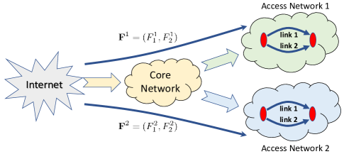
Figure 1: Network used for numerical studies.

IV-A Description of setup

We consider one CN and two ANs - AN 1 and AN 2, as shown in Fig. 1. For the numerical study, we only consider downstream traffic that enters the CN from the Internet and is destined for either AN 1 or AN 2. The networks support two traffic classes, which require different average E2E delay guarantees. The traffic destined for AN $i$ is given by ${\bf F}^{i}=(F^{i}_{1},F^{i}_{2})$, where $F^{i}_{s}$ is the class $s$ traffic destined for AN $i$.

Each AN has two links to carry traffic (links 1 and 2 shown in Fig. 1). The local decision variables of AN $i$ are ${\bf y}_{i}=\big{(}(r^{i}_{\ell,1},r^{i}_{\ell,2},b^{i}_{\ell}):\ell=1,2\big{)}$, where $r^{i}_{\ell,s}$ is the fraction of class $s$ traffic routed through link $\ell$ by AN $i$, and $b^{i}_{\ell}$ is the amount of bandwidth provisioned on link $\ell$ by AN $i$. The cost of AN $i$ comprises (i) the cost of reserving $b^{i}_{\ell}$, $\ell=1,2$, on each link $\ell$ and (ii) the cost that is dependent on the average delays experienced by its traffic. More precisely, the cost of AN $i$, $i=1,2$, is given by

$$\phi_{i}({\bf y}_{i})=\sum_{\ell=1}^{2}\Big{(}p^{i}_{\ell}(b^{i}_{\ell})+\sum_{s=1}^{2}\xi^{i}_{s}(r^{i}_{\ell,s}F^{i}_{s},d^{i}_{\ell}(f^{i}_{\ell},b^{i}_{\ell}))\Big{)},$$ (8)

where $f^{i}_{\ell}=r^{i}_{\ell,1}F^{i}_{1}+r^{i}_{\ell,2}F^{i}_{2}$ is the total flow rate on link $\ell$, $p^{i}_{\ell}$ is the function that determines the total reservation cost on link $\ell$, $d^{i}_{\ell}$ determines the average delay on link $\ell$ as a function of reserved bandwidth and the total flow rate, and $\xi^{i}_{s}$ is the delay cost function of class $s$ traffic.

Similarly, the local decision variables of the CN are the amounts of the bandwidth provisioned for each traffic class and are given by ${\bf y}_{c}=(b_{1},b_{2})$, where $b_{s}$ is the amount of bandwidth reserved for class $s$ traffic. For fixed ${\bf y}_{c}$ and traffic ${\bf F}=(F_{1},F_{2})$, where $F_{s}=F^{1}_{s}+F^{2}_{s}$ is the total amount of class $s$ traffic handled by CN, its cost is given by

$$\phi_{c}({\bf y}_{c}) = \textstyle\sum_{s=1}^{2}\big{(}p_{s}^{c}(b_{s})+\xi^{c}_{s}(F_{s},d^{c}_{s}(F_{s},b_{s}))\big{)},$$ (9)

where $p_{s}^{c}(b_{s})$ is the cost of provisioning bandwidth $b_{s}$ for class $s$ traffic, $d^{c}_{s}$ determines the delay as a function of the total rate and provisioned bandwidth for class $s$ traffic, and $\xi^{c}_{s}$ is the delay cost function for class $s$ traffic.

The CN and the ANs collectively must satisfy constraints on the average E2E delays experienced by the traffic. Specifically, the average E2E delay for traffic class $s$ should not exceed $D_{s}$. This gives rise to the following global constraints:

$$g_{i,s}(\mathbf{y}_{i},\mathbf{y}_{c}) := \frac{1}{F^{i}_{s}}\sum_{\ell=1}^{2}f^{i}_{\ell,s}d^{i}_{\ell}(f^{i}_{\ell},b^{i}_{\ell})+d_{s}^{c}(F_{s},b_{s})-D_{s}\leq 0,$$ (10)

$$\hskip 36.135pti=1,2\ \mbox{ and }\ s=1,2,$$

where $f^{i}_{\ell,s}=r^{i}_{\ell,s}F^{i}_{s}$ is the amount of class $s$ traffic traversing link $\ell$.

The approximated optimization problem we are interested in solving is given by

$$\min_{\mathbf{y}\in{\cal G}}\Big{(}\big{(}\phi_{c}({\bf y}_{c})+\sum_{i=1}^{2}\phi_{i}({\bf y}_{i})\big{)}+\frac{\mu}{6}\sum_{i=1}^{2}\sum_{s=1}^{2}\big{(}[g_{i,s}({\bf y})]_{+}\big{)}^{2}\Big{)}$$ (11)

with decision variables ${\bf y}=({\bf y}_{c},{\bf y}_{1},{\bf y}_{2})$.

IV-B Practical Modifications of the Proposed Algorithm

Our proposed framework and convergence results in Sections II and III, respectively, guarantee the almost sure convergence of the decision variables to an optimal point when the approximated problem in (3) is convex. However, there are a few practical issues that one should consider, which are discussed here.

$\bullet$ Modification 1 – While the step sizes $\gamma_{t}$, $t\in{\rm I\kern-2.5ptN}$, can be chosen sufficiently small to avoid large fluctuations in the decision variables, which are updated in accordance with (4) and (6), selecting small step sizes also hampers their convergence to the optimal set. In order to skirt this issue, we apply a limiter to (some elements of) $\gamma_{t}{\bf U}_{i}(t)$ in (4). Specifically, we use the limiter to the elements corresponding to the routing probabilities $r^{i}_{\ell,s}$ so that the elements of $\gamma_{t}{\bf U}_{i}(t)$ corresponding to these decision variables always lie in [-0.01, 0.01]. The use of such limiters alters our proposed algorithm from that described in Section II. However, the almost sure convergence to the optimal set shown in Section III still holds with the modified algorithm under the assumed Lipschitz continuity of gradients functions and bounded noise.

$\bullet$ Modification 2 – We observe from (5) that when agent $i$’s estimate of the $k$th global constraint at iteration $t$, namely $e_{i,k}(t)$, is positive, it introduces the corresponding term $\mu\nabla g_{i,k}({\bf y}(t))[e_{i,k}(t)]_{+}$ in the update term used in (4). Hence, when $e_{i,k}(t)$ oscillates around zero, it is added to the update term whenever $e_{i,k}(t)>0$ while it makes no contribution to the update term when $e_{i,k}(t)\leq 0$, causing a non-negligible change in the update term. This is undesirable and slows down the convergence of decision variables.

In order to cope with this issue, rather than using the true delay budgets $D_{s},s=1,2$, we use target delay budgets equal to $D^{T}_{s}=\tau D_{s}$, where $\tau\in(0,1]$. We call the global constraints with the delay budgets replaced by the target delay budgets the fictitious global constraints. The main idea behind the use of fictitious global constraints is two-fold. First, satisfying the global constraints with true delay budgets in general requires selecting a large penalty parameter, which increases the sensitivity to the constraint function values (and their estimates). Second, using fictitious constraint functions allows us to use a smaller penalty parameter (hence, reduces the aforementioned sensitivity to the global constraint function values); we can violate the fictitious delay constraints while still satisfying the true delay constraints. This implies that the agents’ estimates of fictitious constraint functions stay positive, avoiding the aforementioned oscillations, while still satisfying the original global constraints.

IV-C Numerical Results

In our numerical study, we assumed following functions:

$$d^{i}_{\ell}(f,b)=\upsilon_{\ell}\big{(}f/b\big{)}^{a},\ d_{s}^{c}(f,b)=\big{(}f/b\big{)}^{a},p^{i}_{\ell}(b)=\kappa^{i}_{\ell}\cdot b^{k},$$

$$p_{s}^{c}(b)=\kappa_{s}\cdot b^{k},\ \xi^{c}_{s}(f,d)=\beta_{s}fd,\ \mbox{and}\ \xi^{i}_{s}(f,d)=\beta^{i}_{s}fd,$$

where $\kappa^{i}_{\ell}>0$, $\kappa_{s}>0$, $\gamma_{s}>0$, $\beta^{i}_{s}>0$, $a\geq 1$ and $k\geq 1$. The following parameter values are used in the study:

$$\upsilon_{1}=1,\ \upsilon_{2}=0.8,\ \kappa^{1}_{1}=4,\ \kappa^{1}_{2}=5,\ \kappa^{2}_{1}=7,\ \kappa^{2}_{2}=9,$$

$$\kappa_{1}=4,\ \kappa_{2}=6,a=2.5,\ k=1.1,\ \beta^{i}_{1}=\beta_{1}=40,$$

$$\mbox{ and }\ \beta^{i}_{2}=\beta_{2}=10,\ i=1,2.$$

The flow rates are ${\bf F}^{1}=(40,20)$ and ${\bf F}^{2}=(50,30)$. The delay budgets are chosen to be $D_{1}=0.7$ and $D_{2}=0.5$ with the target delay budgets set to 60 percent of the true delay budgets, which are $D^{T}=(0.42,0.3)$. The penalty parameter is set to $2\cdot 10^{4}$: a relatively large value of penalty parameter is necessary in our scenario because the delay budgets are much smaller than the costs of reserving bandwidth for the networks. The employed doubly-stochastic weight matrix $W:=[w_{ij}:i,j\in\{c,1,2\}]$ used in (6) is given by

$$W=\begin{bmatrix}3/4&1/8&1/8\\ 1/8&7/8&0\\ 1/8&0&7/8\end{bmatrix}.$$

The stochastic perturbation ${\bf V}_{i}(t)$ introduced in the noisy observation of gradient is uniformly distributed over $[-\sigma\nabla\phi_{i}(\mathbf{y}_{i}(t)),\sigma\nabla\phi_{i}(\mathbf{y}_{i}(t))]$. For the reported numerical results, we pick $\sigma=0.75$. The step sizes are selected to be $\gamma_{t}=\min(0.1,(t+1)^{-0.6})$, $t\in{\rm I\kern-2.5ptN}$. Finally, the decision variables are initialized as follows. Let $F^{i}=\sum_{s=1}^{2}F^{i}_{s}$, $i=1,2$, and $F^{T}=F_{1}+F_{2}=F^{1}+F^{2}$:

$$\mathbf{y}_{c}=(B_{1},B_{2}),\ \mathbf{y}_{1}=(0.5,0.5,0.5,0.5,B^{1}_{1},B^{1}_{2}),$$

$$\mbox{and }\ \mathbf{y}_{2}=(0.5,0.5,0.5,0.5,B^{2}_{1},B^{2}_{2}),$$

where $B_{s}\sim$ Uniform($0,2F^{T}$), $s=1,2$, and $B^{i}_{\ell}\sim$ Uniform($F^{i},2F^{i}$), $i=1,2$ and $\ell=1,2$. These random variables are selected independently.

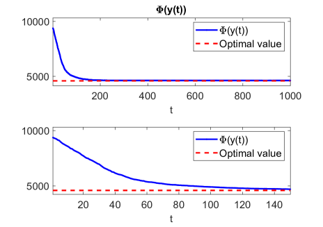
Figure 2: Plot of the objective function $\Phi(\mathbf{y}(t))$.

First, we plot the value of the objective function $\Phi(\mathbf{y}(t))$ of the approximated optimization problem in (11) for $t$ in {1, 2, …, 1000} (top) and {1, 2, …, 150} (bottom) in Fig. 2. The dotted red lines represent the optimal value we obtained using the MATLAB optimization tool. The plots suggest that the value of $\Phi(\mathbf{y}(t))$ converges to the optimal value quickly. In fact, the bottom plot indicates that we are within 2-3 percent of the optimal value within 150 iterations, despite large noises.

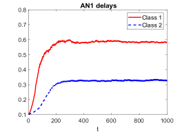
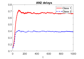
Figure 3: End-to-end delays experienced by traffic traversing to AN 1 (left) and AN 2 (right).

Fig. 3 plots the realized E2E delays experienced by the traffic destined for AN 1 (left) and AN 2 (right). With the employed parameters, the true delay constraints are satisfied for both traffic classes. In contrast, when there is no penalty function, the realized E2E delays for class 1 and 2 traffic destined for AN 1 (resp. AN 2) are 3.7 and 8.7 (resp. 5.6 and 10.6), respectively. Obviously, these numbers are many times larger than their delay budgets and, hence, are unacceptable.

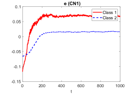
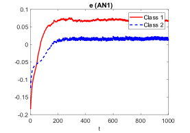
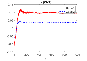
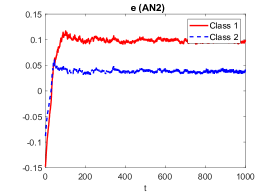
Figure 4: Estimates of constraint functions maintained by agents.

Recall that the E2E target delay budgets for class 1 and 2 traffic are $D^{T}_{1}=0.42$ and $D^{T}_{2}=0.3$, respectively. The delays experienced by the traffic destined for AN 1 in the left plot of Fig. 3, which include the delays in both the CN and AN 1, exceed the target delays by approximately 0.17 and 0.03 for class 1 and 2 traffic, respectively. Hence, according to (7), the estimates of the agents must be approximately 0.06 and 0.01. Similarly, according to the right plot in Fig. 3, the agents’ estimates for class 1 and 2 traffic should be approximately 0.1 and 0.03. Fig. 4 shows the estimates $\mathbf{e}_{i}(t)$, $i\in\{c,1,2\}$; the top figures (resp. bottom figures) are the estimates of $g_{1,s}$ (resp. $g_{2,s}$), $s=1,2$. It is clear from the figure that the agents are indeed able to closely track the average constraint function values using the proposed consensus-type algorithm in (6).

V Discussion: Relation to Nash Equilibria of A State-Based Potential Game

In the previous sections, we implicitly assumed that the agents are willing to employ the proposed algorithm to cooperate in order to satisfy global constraints. In general, the agents will adopt the proposed algorithm only if they believe that they cannot reduce their own costs without significantly increasing global constraint violations by deviating from the equilibrium, i.e., an optimal point of (3). It turns out that there is a close relation between an optimal point of (3) and a Nash equilibrium of a state-based potential game (SBPG) associated with the problem.

An SBPG consists of the following [18]:

• a set of agents ${\cal A}$;

• a state space ${\cal X}$;

• for each agent $i\in{\cal A}$ and each state ${\bf x}\in{\cal X}$, (i) a state-dependent admissible action set ${\cal Y}_{i}({\bf x})$ and (ii) a state-dependent cost function $J_{i}$, where $J_{i}({\bf x},{\bf a})$ is agent $i$’s cost at the state ${\bf x}$ when the agents adopt action profile ${\bf a}\in\prod_{i\in{\cal A}}{\cal Y}_{i}({\bf x})=:{\cal Y}({\bf x})$; and

• a deterministic state transition function $f$: given the current state ${\bf x}$ and agents’ action profile ${\bf a}\in{\cal Y}({\bf x})$, the next state is given by $f({\bf x},{\bf a})\in{\cal X}$.

There is also a null action profile ${\bf a}^{0}$ such that ${\bf a}^{0}\in{\cal Y}({\bf x})$ and ${\bf x}=f({\bf x},{\bf a}^{0})$ for all ${\bf x}\in{\cal X}$. In other words, the state does not change when the agents adopt the null action profile. A state-action pair $({\bf x}^{\star},{\bf a}^{\star})$ is said to be a stationary state Nash equilibrium of the SBPG if (i) $a_{i}^{\star}\in\arg\min_{a_{i}\in{\cal Y}_{i}({\bf x}^{\star})}J_{i}\big{(}{\bf x}^{\star},(a_{i},{\bf a}_{-i}^{\star})\big{)}$ for every agent $i\in{\cal A}$, where ${\bf a}_{-i}^{\star}$ is the action profile of all agents except for agent $i$, i.e., ${\bf a}_{-i}^{\star}=(a_{j}^{\star}:j\in{\cal A}\setminus\{i\})$, and (ii) ${\bf x}^{\star}=f({\bf x}^{\star},{\bf a}^{\star})$.

Consider a game with the state given by ${\bf x}=({\bf y},{\bf e})$, where ${\bf y}$ is the vector of decision variables in our optimization problem, and ${\bf e}=({\bf e}_{i}:i\in{\cal A})$ is the vector of constraint function estimates. Given a state ${\bf x}\in{\cal X}$, an action $a_{i}$ of agent $i$ is a tuple $\big{(}\hat{{\bf y}}_{i},(\hat{{\bf e}}_{i\to j}:j\in{\cal N}_{i})\big{)}$, where $\hat{{\bf y}}_{i}$ is the change in agent $i$’s decision variables and $\hat{{\bf e}}_{i\to j}$ is the estimates of constraint functions agent $i$ forwards to its neighbor $j\in\mathcal{N}_{i}:=\{j\in{\cal A}\ |\ w_{ij}>0\}$. Suppose that the state transitions to a new state based on the current state ${\bf x}$ and the chosen action profile ${\bf a}$ as follows:

$$\overline{{\bf y}}_{i} = {\bf y}_{i}+\hat{{\bf y}}_{i}$$

$$\overline{{\bf e}}_{i} = {\bf e}_{i}+{\bf g}_{i}(\overline{{\bf y}}_{i})-{\bf g}_{i}({\bf y}_{i})+\textstyle\sum_{j\in{\cal N}_{i}}\big{(}\hat{{\bf e}}_{j\to i}-\hat{{\bf e}}_{i\to j}\big{)}.$$

Consider the cost function of agent $i$ given by

$$J_{i}({\bf x},\mathbf{a})=\phi_{i}(\overline{\mathbf{y}}_{i})+\frac{\mu}{2}\textstyle\sum_{j\in\mathcal{N}_{i}}\|[\overline{\mathbf{e}}_{j}]_{+}\|_{2}^{2},$$ (12)

where $\mu>0$ is a trade-off parameter. This gives rise to an SBPG with a global potential function given by [16]

$$\Phi_{\mu}({\bf x},\mathbf{a})=\textstyle\sum_{i\in\mathcal{A}}\phi_{i}(\overline{\mathbf{y}}_{i})+\frac{\mu}{2}\textstyle\sum_{i\in\mathcal{A}}\|[\overline{\mathbf{e}}_{i}]_{+}\|_{2}^{2}.$$ (13)

Note the similarity between the objective function in (3) and the global potential function in (13). From (7), we have ${\bf g}({\bf y}(t))=\sum_{i\in{\cal A}}{\bf g}_{i}({\bf y}_{i}(t))=\sum_{i\in{\cal A}}{\bf e}_{i}(t)$. Hence, when all agents have the correct estimate of the average constraint function values, i.e., ${\bf e}_{i}(t)={\bf e}_{\rm avg}(t)$ for all $i\in{\cal A}$, the global potential function coincides with the objective function in (3) with a different penalty parameter. This observation can be used to prove the following proposition.

Proposition 1

Suppose that ${\bf y}^{*}\in{\cal Y}^{*}$ is an optimal point of (3). Then, $\big{(}({\bf y}^{*},\mathbf{g}({\bf y}^{*})/N),\mathbf{0}\big{)}$, where $\mathbf{0}$ is the null action profile, is a stationary state Nash equilibrium of the SBPG.

The above proposition means that each optimal point in ${\cal Y}^{*}$ leads to a stationary state Nash equilibrium and there is an one-to-one mapping from ${\cal Y}^{*}$ to a set of stationary state Nash equilibria of the SBPG.

VI Conclusions

We proposed a novel distributed algorithm that enables autonomously managed ANs and CNs in a telecommunication system to cooperate with each other to meet E2E KPI goals. The new algorithm overcomes two major limitations of prior techniques. First, unlike prior approaches that require static local KPI budgets for each autonomous subsystem, the new algorithm allows the autonomous subsystems to dynamically negotiate their local KPI budgets. Second, rather than requiring the autonomous subsystems to share their local decision variables with each other, our proposed algorithm only needs the subsystems to exchange their estimates of the global constraint functions. We proved that the new algorithm converges to an optimal solution almost surely, and presented numerical results to demonstrate that the convergence occurs quickly even with measurement noise.

References

- [1] 3GPP TS 22.261 V15.8.0 (2019-09), “3rd Generation Partnership Project; Technical Specification Group Services and System Aspects; Service requirements for the 5G system; Stage 1 (Release 15).”
- [2] 3GPP TS 23.501 V15.12.0 (2020-12), “3rd Generation Partnership Project; Technical Specification Group Services and System Aspects; System architecture for the 5G System (5GS); Stage 2 (Release 15).”
- [3] 3GPP TS 28.550 V16.1.0 “Management and orchestration; Performance assurance”.
- [4] 3GPP TS 28.552 V16.1.0 “Management and orchestration; 5G performance measurements”.
- [5] 3GPP TS 28.554 V16.0.0 “Management and orchestration; 5G end to end Key Performance Indicators (KPI)”.
- [6] 3GPP TS 32.425 V16.3.0 “Performance Management (PM); Performance measurements for Evolved Universal Terrestrial Radio Access Network (E-UTRAN)”.
- [7] 3GPP TS 28.532 V16.0.0 “Management and orchestration; Generic management services”.
- [8] M. Asad, A. Basit, S. Qaisar and M. Ali, “Beyond 5G: Hybrid End-to-End Quality of Service Provisioning in Heterogeneous IoT Networks,” IEEE Access, 8:192320-192338, 2020, doi: 10.1109/ACCESS.2020.3032704.
- [9] P. Bianchi and J. Jakubowicz, “Convergence of a multi-agent projected stochastic gradient algorithm for non-convex optimization,” IEEE Trans. on Automatic Control, 58(2):391-405,
- [10] S. Boyd and L. Vandenberghe, Convex Optimization, Cambridge University Press, 2004.
- [11] D. L. C. Dutra, M. Bagaa, T. Taleb and K. Samdanis, “Ensuring End-to-End QoS Based on Multi-Paths Routing Using SDN Technology,” Proc. of IEEE GLOBECOM, Singapore, 2017, pp. 1-6, doi: 10.1109/GLOCOM.2017.8254076.
- [12] R. Jacquet, G. Texier and A. Blanc, “Computing end-to-end QoS paths in the Internet considering multiple alliances,” Proc. of the 16th International Telecommunications Network Strategy and Planning Symposium (Networks), 2014, pp. 1-6, doi: 10.1109/NETWKS.2014.6959248.
- [13] H. Kushner and G. Yin, Stochastic Approximation and Recursive Algorithms and Applications, 2nd ed. Springer, 2003.
- [14] Y. Lee, K. John and R. Vilalta, “Extended ACTN Architecture to Enable End-To-End 5G Transport Service Assurance,” Proc. of the 21st International Conference on Transparent Optical Networks (ICTON), Angers, France, 2019, pp. 1-3, doi: 10.1109/ICTON.2019.8840270.
- [15] K. B. Letaief, W. Chen, Y. Shi, J. Zhang and Y. A. Zhang, “The Roadmap to 6G: AI Empowered Wireless Networks,” IEEE Communications Magazine, 57(8):84-90, Aug. 2019, doi: 10.1109/MCOM.2019.1900271.
- [16] N. Li and J.R. Marden, “Decoupling coupled constraints through utility design,” IEEE Trans. on Automatic Control, 59(8):2289-=2294, Aug. 2014.
- [17] V. S. Mai, R. J. La, T. Zhang and A. Battou, “Distributed Optimization with Global Constraints Using Noisy Measurements,” arXiv preprint arXiv:2106.07703, 2021.
- [18] J. Marden and J. S. Shamma, “Game theory and distributed control,” Handbook of Game Theory with Economic Applications, pp. 861-899, 2015.
- [19] W. Saad, M. Bennis and M. Chen, “A Vision of 6G Wireless Systems: Applications, Trends, Technologies, and Open Research Problems,” IEEE Network, vol. 34(3):134-142, May/June 2020, doi: 10.1109/MNET.001.1900287.
- [20] C. She et al., “Deep Learning for Ultra-Reliable and Low-Latency Communications in 6G Networks,” IEEE Network, 34(5):219-225, Sep./Oct. 2020, doi: 10.1109/MNET.011.1900630.
- [21] K. Srivastava and A. Nedi, “Distributed asynchronous constrained stochastic optimization,” IEEE Journal of Selected Topics in Signal Processing, 5(4:)772-790, 2011.
- [22] C.-C. Teng, M.-C. Chen, M.-H. Hung and H.-J. Chen, “End-to-end Service Assurance in 5G Crosshaul Networks,” Proc. of the 21st Asia-Pacific Network Operations and Management Symposium (APNOMS), Daegu, Korea (South), 2020, pp. 306-309, doi: 10.23919/APNOMS50412.2020.9236977.
- [23] Q. Ye, J. Li, K. Qu, W. Zhuang, X. S. Shen and X. Li, “End-to-End Quality of Service in 5G Networks: Examining the Effectiveness of a Network Slicing Framework,” IEEE Vehicular Technology Magazine, 13(2):65-74, Jun. 2018, doi: 10.1109/MVT.2018.2809473.
- [24] T. Zhang, “Toward Automated Vehicle Teleoperation: Vision, Opportunities, and Challenges,” IEEE Internet of Things Journal, 7(12):11347-11354, Dec. 2020, doi: 10.1109/JIOT.2020.3028766.
- [25] G. Zhu, J. Zan, Y. Yang and X. Qi, “A Supervised Learning Based QoS Assurance Architecture for 5G Networks,” IEEE Access, 7:43598-43606, 2019, doi: 10.1109/ACCESS.2019.2907142.