Non-Markovian feedback control and acausality: an experimental study

Abstract

Causality is an important assumption underlying nonequilibrium generalizations of the second law of thermodynamics known as fluctuation relations. We here experimentally study the nonequilibrium statistical properties of the work and of the entropy production for an optically trapped, underdamped nanoparticle continuously subjected to a time-delayed feedback control. Whereas the non-Markovian feedback depends on the past position of the particle for a forward trajectory, it depends on its future position for a time-reversed path, and is therefore acausal. In the steady-state regime, we show that the corresponding fluctuation relations in the long-time limit exhibit a clear signature of this acausality, even though the time-reversed dynamics is not physically realizable.

There is a direct relationship between heat dissipation and irreversibility of a thermodynamic process, as expressed by the breaking of time-reversal symmetry. Consider, for example, a classical system in contact with a thermal bath, such as a Brownian particle driven arbitrarily far from equilibrium by an external perturbation. The heat exchanged with the bath along a particular stochastic trajectory (starting from a given initial state) can then be expressed as the logratio of the probabilities of the trajectory and of the corresponding time-reversed path, with the time-reversed protocol [1]. This fundamental property, referred to as microscopic reversibility [2], ensures the thermodynamic consistency of the dynamics at the level of fluctuating trajectories. It is at the origin of most fluctuation relations, which are the cornerstones of our modern understanding of out-of-equilibrium processes [3, 2, 4, 1, 5].

Matters are more complicated when information is extracted from the system to regulate or modify its state via feedback control [6, 7, 8, 9, 10, 11, 12, 13]. Feedback operation is widespread in many biological systems and technological applications [14, 15, 16, 17]. Non-Markovian effects induced by the unavoidable time lag between signal detection and control action then raise a fundamental question: how should the time-reversed process, associated with microscopic reversibility, be defined? Should the reversed dynamics be implemented without measurement and feedback, which is the solution advocated for Szilárd-type engines [9, 7, 8]? Or should the two still be present? In the latter case, microscopic reversibility is modified, as the fluctuating heat is no longer odd under time reversal [18, 19, 20]. Since feedback action depends on the future state of the system for the backward process, causality is violated (Fig. 1). Still, this strategy is claimed to provide a consistent description of the stochastic thermodynamics [18, 19, 20]. But there is a price to pay: the backward process is no longer physically realizable.

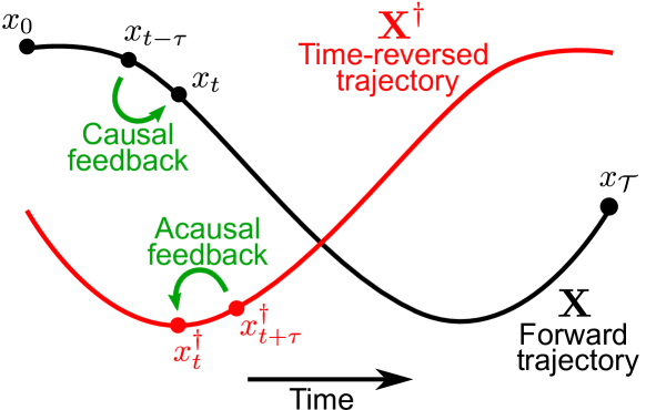
Figure 1: Schematic representation of a path ${\bf X}=\{x_{t}\}_{0\leq t\leq{\cal T}}$ and its time-reversal ${\bf X}^{\dagger}=\{x_{{\cal T}-t}\}_{0\leq t\leq{\cal T}}$. While the time-delayed feedback control depends on the past position of the particle $x_{t-\tau}$ (causal feedback) for the forward trajectory, it depends on the future position of the particle $x^{\dagger}_{t+\tau}$ (acausal feedback) for the time-reversed path.

In this paper, we report the first experimental evidence that the acausal backward dynamics is a useful tool that allows us to predict properties of real physical systems. To this end, we use a setup consisting of a levitated nanoparticle trapped in a harmonic potential and subjected to a position-dependent time-delayed feedback [21, 22]. Owing to the continuous feedback, the system settles in a nonequilibrium steady state where heat is permanently exchanged with the bath. We then record the fluctuations of two trajectory observables: the work ${\cal W}_{{\cal T}}$ done by the feedback force within a time window of duration ${\cal T}$ and the corresponding entropy production $\Sigma_{\cal T}$. Whereas the expectation values of these quantities are identical, their fluctuations far away from the mean may differ, due to rare events associated with temporal boundary terms. Their statistics, moreover, depend on the delay [18, 19, 20]. A remarkable conjecture is that $\Sigma_{\cal T}$ satisfies asymptotically the fluctuation relation [18, 19, 20]

$$\langle e^{-\Sigma_{{\cal T}}}\rangle\sim e^{\dot{S}_{J}{\cal T}}\ ,\>\>({\cal T}\to\infty)\ ,$$ (1)

where $\dot{S}_{J}$ is a “Jacobian” contribution induced by the breaking of causality in the backward process (the theoretical analysis is summarized in the Supplemental Material [23]). The rate $\dot{S}_{J}$ is an upper bound to the extracted work [19] and may be viewed as an entropic cost of the non-Markovian feedback. When the acausal backward dynamics allows for the existence of a stationary state, the work ${\cal W}_{{\cal T}}$ is predicted to similarly obey $\langle e^{-\beta{\cal W}_{{\cal T}}}\rangle{\sim}e^{\dot{S}_{J}{\cal T}}$, with $\beta=1/(k_{B}T)$ and $T$ the bath temperature) [20, 23].

In the following, we experimentally check the validity of these two asymptotic fluctuation relations. A confirmation of these conjectures would open the door to an experimental determination of the acausal contribution $\dot{S}_{J}$, whose explicit expression for general non-Markovian Langevin systems is out of reach [24]. However, estimating an exponential average from experimental time series is a daunting task, as illustrated by the computation of the equilibrium free energy from the Jarzynski equality [25]. The main problem is that the average is dominated by very rare realizations [26], which by definition are hard to get in experiments [27]. Obtaining the genuine asymptotic behavior is even more challenging since it becomes exponentially more unlikely to observe fluctuations away from the mean as ${\cal T}$ increases. This is the major difficulty we have to address and this forces us to perform a delicate statistical analysis of the behavior of $\langle e^{-\Sigma_{{\cal T}}}\rangle$ and $\langle e^{-\beta{\cal W}_{{\cal T}}}\rangle$ as a function of the time ${\cal T}$.

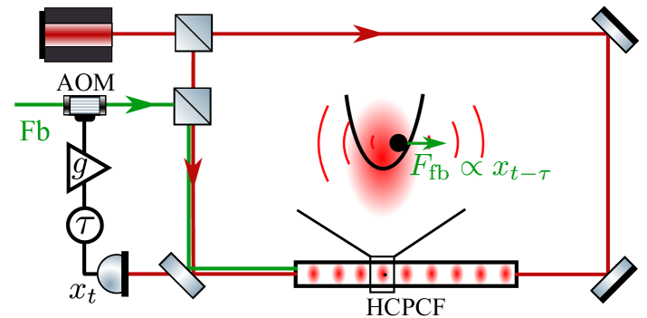
Figure 2: Experimental setup. A nanoparticle is levitated in a harmonic optical trap formed by two counter-propagating beams (red), inside a hollow-core photonic crystal fiber. The nanoparticle is subjected to a delayed feedback force $F_{\text{fb}}\propto x_{t-\tau}$ implemented with an acousto-optic modulator using radiation pressure from an additional laser beam (green). The feedback loop is characterized by a gain $g$ and time delay $\tau$.

Experimental setup. We consider a levitated nanoparticle (295 nm diameter) trapped at an intensity maximum of a standing wave formed by two counterpropagating laser beams ($\lambda=1064$ nm) inside a hollow-core photonic crystal fiber [21, 22] (Fig. 2). The particle oscillates in the harmonic trap with a resonance frequency $f_{0}=\Omega_{0}/2\pi=297.7$ kHz and is damped by the surrounding gas at temperature $T=293$ K with a damping rate $\Gamma_{0}/2\pi=5.93$ kHz. The quality factor of the oscillator is $Q_{0}=\Omega_{0}/\Gamma_{0}=50.2$. The particle motion along the fiber axis ($x$-axis) is detected by interferometric readout of the light scattered by the particle, with a position sensitivity of 2 pm/$\sqrt{\text{Hz}}$ [21]. A variable delay $\tau$ is then added to the position signal using a field-programmable gate array and a feedback force $F_{\text{fb}}\propto x_{t-\tau}$ is applied to the nanoparticle via radiation pressure. The feedback loop has a variable gain $g$ and an internal minimum delay of $3~{}\mu$s mainly due to the acousto-optic modulator and the band pass filter of the feedback loop. For each of the 19 chosen delays $\tau$, we record a long trajectory of duration $\mathcal{T}_{\text{tot}}=1000\>$s with a sampling rate of $5$ MHz. This amounts to 5 hours total data acquisition time, which is short enough to keep experimental drifts small (estimated relative uncertainties: ${\Delta\Gamma_{0}}/{\Gamma_{0}}\leq 2\%$ and ${\Delta g}/{g}\leq 5\%$). We also account for the change of sensitivity of the detector by normalizing each raw value of the particle position by the laser power. The data is filtered with a $\pm 150$ kHz bandwidth digital filter around $\Omega_{0}$ to eliminate low frequency technical noise.

For small displacements, the motion of the particle is described by an underdamped Langevin equation [29],

$$\ddot{x}_{t}+\Gamma_{0}\dot{x}_{t}+\Omega_{0}^{2}x_{t}-g\Gamma_{0}\Omega_{0}x_{t-\tau}=\sqrt{\frac{2\Gamma_{0}k_{B}T}{m}}\xi_{t},$$ (2)

where $m$ is the mass and $\xi(t)$ is the Gaussian thermal noise, delta-correlated in time with variance $1$. The feedback force is $F_{\text{fb}}=-g(m\Gamma_{0}\Omega_{0})x_{t-\tau}$ with $g>0$. Hereafter, we shall use $\Omega_{0}^{-1}$ and $x_{0}=(1/\Omega_{0}^{2})(2\Gamma_{0}k_{B}T/m)^{1/2}$ as units of time and position, respectively [18, 19, 20]. The dynamics of the particle is then characterized by the dimensionless parameters $(g,Q_{0},\tau)$ [30]. We further express the observation time ${\cal T}$ in units of $Q_{0}$, that is, as a multiple of the relaxation time $\Gamma_{0}^{-1}$.

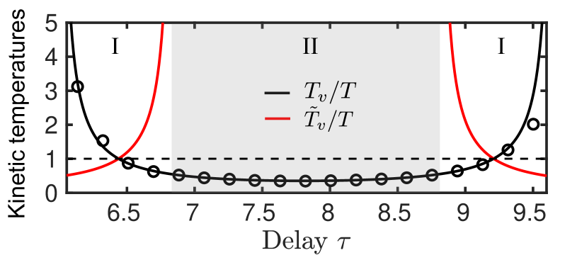
Figure 3: Steady-state kinetic temperatures versus time delay in the second stability region of the oscillator (in units of $\Omega_{0}^{-1}$). The black solid line is the theoretical prediction for the (causal) temperature ratio $T_{v}/T$ and symbols are data obtained by averaging $v^{2}_{t}$ over a trajectory of length $1000Q_{0}$. The red solid line is the prediction for the (acausal) temperature ratio ${\widetilde{T}}_{v}/T$ in the region (labelled I) where the acausal dynamics admits a stationary solution.

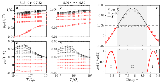
Figure 4: (a-d) Estimates of $\mu_{W}(1,{\cal T})$ (squares) and $\mu_{\Sigma}(1,{\cal T})$ (stars) as a function of the observation time ${\cal T}$ (in unit of $\Omega_{0}^{-1}$), for various delays $\tau$. Panels (a) and (c): from bottom to top, $\tau=6.13,6.32,6.51,6.70$ (red) and $\tau=6.88,7.07,7.26,7.44,7.63,7.82$ (black). Panels (b) and (d): from top to bottom, $\tau=8.00,8.19,8.38,8.57,8.75$ (black) and $\tau=8.94,9.13,9.31,9.50$ (red). Solid lines are a guide to the eye. e) Values of $\mu_{\Sigma}(1)$ (stars) and $\mu_{\mathcal{W}}(1)$ (squares) deduced from the data plotted in panels (a)-(d). The solid line is the theoretical expression of the acausal contribution $\dot{S}_{J}$ [19, 23]. In region I (red symbols), the acausal dynamics has a stationary solution and $\mu_{\Sigma}(1)=\mu_{W}(1)=\dot{S}_{J}$. In region II (black symbols), $\mu_{W}(1)=1/Q_{0}$ and $\mu_{\Sigma}(1)=\dot{S}_{J}$. f) Ratio of the pre-exponential factors $g_{W}(1)/g_{\Sigma}(1)$ in region I. The red solid line is the conjectured formula (5). Error bars are discussed in the Supplemental Material [23].

The feedback-controlled oscillator has a complex dynamical behavior and may exhibit multistability [19]. We choose a feedback gain $g=2.4$ so as to probe the two regimes that differentiate the fluctuations for ${\cal W}_{{\cal T}}$ and $\Sigma_{{\cal T}}$ (Fig. 4). We moreover select values of $\tau$ between 6.13 and 9.50 (i.e. between $3.28\>\mu$s and $5.08\>\mu$s) that correspond to the second stability region [23]. The viscous relaxation time ($\Gamma_{0}^{-1}\approx 27\mu$s) is much larger than the considered delays, ensuring the efficiency of the feedback loop. This is quantified by the kinetic temperature of the particle, defined as $T_{v}=(2T/Q_{0})\langle v^{2}_{t}\rangle$ in reduced units, which determines the average heat flow into the environment, $\langle\beta\dot{Q}\rangle=(1/Q_{0})(T_{v}/T-1)$ [19, 22]. As seen in Fig. 3, the experimental values of $T_{v}$ computed from the mean-square velocity (black symbols) are in excellent agreement with the theoretical predictions (black lines) [19]. In particular, the feedback cooling regime, $T_{v}/T<1$, and thus $\langle\dot{Q}\rangle<0$, is achieved for $6.44\lesssim\tau\lesssim 9.21$.

Asymptotic fluctuation relations for work and entropy production. The stochastic work ${\cal W}_{{\cal T}}$ performed by the feedback force along a trajectory of duration ${\cal T}$ is

$$\beta{\cal W}_{{\cal T}}=\frac{2g}{Q_{0}^{2}}\int_{0}^{{\cal T}}dt\>x_{t-\tau}\circ v_{t}\ ,$$ (3)

where the integral is interpreted with the Stratonovich prescription [31]. The corresponding entropy production (EP) is defined as [23]

$$\Sigma_{{\cal T}}=\beta{\cal Q}_{{\cal T}}+\ln\frac{p(x_{0},v_{0})}{p(x_{{\cal T}},v_{{\cal T}})}\ ,$$ (4)

where ${\cal Q}_{{\cal T}}=(2/Q_{0})\int_{0}^{{\cal T}}dt\>[v_{t}/Q_{0}-\xi(t)]\circ v_{t}$ is the heat dissipated into the environment [31] and $p(x,v)$ is the stationary probability distribution. Note that $\langle e^{-\Sigma_{{\cal T}}}\rangle\neq 1$ and that $\langle\Sigma_{{\cal T}}\rangle<0$ in the cooling regime, which may look as a violation of the second law. But $\Sigma_{{\cal T}}$ is just the “apparent” stochastic EP which an observer unaware of the existence of the feedback loop would naively regard as the total EP [32]. The important point is that $\Sigma_{{\cal T}}$ is an experimentally accessible quantity.

To simplify the analysis, we rewrite Eq. (1) as $\mu_{\Sigma}(1)=\dot{S}_{J}$ where $\mu_{\Sigma}(\lambda)=\lim_{{\cal T}\to\infty}(1/{\cal T})\ln\langle e^{-\lambda\Sigma_{{\cal T}}}\rangle$ is the scaled cumulant generating function [33]. Likewise, $\mu_{W}(1)=\dot{S}_{J}$ when the acausal dynamics converges to a stationary state. Correctly estimating these two quantities from experiments requires a large amount of data. We use a block-averaging approach, dividing the full time series $\{x_{t}\}_{0\leq t\leq{\cal T}_{\text{tot}}}$ into $N$ blocks of length ${\cal T}$ [23]. We then compute the observables in each block, and approximate $\langle e^{-\Sigma_{{\cal T}}}\rangle$ and $\langle e^{-\beta{\cal W}_{{\cal T}}}\rangle$ with the averages over the $N$ blocks. Obviously, a large value of ${\cal T}$ implies a small ensemble size $N$, resulting in a poor estimation of the empirical averages. There is no perfect solution to this conundrum [28], but we found preferable to use a large value of $N$ and study the two quantities $\mu_{\Sigma}(1,{\cal T})=(1/{\cal T})\ln\langle e^{-\Sigma_{{\cal T}}}\rangle$ and $\mu_{W}(1,{\cal T})=(1/{\cal T})\ln\langle e^{-\beta{\cal W}_{{\cal T}}}\rangle$ as a function of the observation time ${\cal T}$. We then analyze their large-time limits by fitting them for finite $\mathcal{T}$ and extrapolating the results to $\mathcal{T}\to\infty$ (see Ref. [34] for a similar procedure).

Results. The estimates of $\mu_{\Sigma}(1,{\cal T})$ and $\mu_{W}(1,{\cal T})$ are presented in Figs. 4a,c for $6.13\leq\tau\leq 7.82$ and Figs. 4b,d for $8.00\leq\tau\leq 9.50$. The ensemble size is $N=5\cdot 10^{6}$ for ${\cal T}\leq 5Q_{0}$ and $N=3\cdot 10^{6}$ for ${\cal T}=10Q_{0}$. We observe that $\mu_{\Sigma}(1,{\cal T})$ and $\mu_{W}(1,{\cal T})$ behave differently with ${\cal T}$. This is due to contributions of the boundary term in $\Sigma_{{\cal T}}$. More interesting is the fact that two regimes, hereafter labelled I and II, can be distinguished as a function of the delay: In regime I (red symbols in Figs. 4a-d), both $\mu_{\Sigma}(1,{\cal T})$ and $\mu_{W}(1,{\cal T})$ vary more or less monotonically with ${\cal T}$ and the values for the largest observation time depend on $\tau$. By contrast, in regime II (black symbols), these values are independent of $\tau$ and very close to $1/Q_{0}\approx 0.02$. Moreover, $\mu_{\Sigma}(1,{\cal T})$ first increases with ${\cal T}$, then reaches a plateau, and ultimately decreases to $1/Q_{0}$. We will argue below that this decrease is induced by the finite statistics of rare events.

The existence of two regimes suggests an intriguing connection with the acausal dynamics obtained by changing $x_{t-\tau}$ into $x_{t+\tau}$ in Eq. (2). Indeed, this dynamics admits a stationary solution for $6.00\lesssim\tau\lesssim 6.85$ and $8.80\lesssim\tau\lesssim 9.66$ [23]. This “acausal” stationary state is characterized by finite values of $\langle x^{2}_{t}\rangle$ and $\langle v^{2}_{t}\rangle$, and thus well-defined “acausal” configurational and kinetic temperatures $\widetilde{T}_{x}$ and $\widetilde{T}_{v}$ [20, 23]. This is illustrated in Fig. 3 that shows the variations of ${\widetilde{T}}_{v}$ with $\tau$.

In this regime I, theory predicts that $\mu_{\Sigma}(1)=\mu_{W}(1)=\dot{S}_{J}$ [20]. To experimentally check these conjectures, we write $\langle e^{-\Sigma_{{\cal T}}}\rangle{\sim}g_{\Sigma}(1)\,e^{\mu_{\Sigma}(1){\cal T}}$ and $\langle e^{-{\cal W}_{{\cal T}}}\rangle{\sim}g_{W}(1)\,e^{\mu_{W}(1){\cal T}}$ for ${\cal T}$ sufficiently large [35], and we fit $\mu_{\Sigma}(1,{\cal T})$ and $\mu_{W}(1,{\cal T})$ with $a+b/{\cal T}+c/{\cal T}^{2}$ in the range $1\leq{\cal T}/Q_{0}<10$ [23]. We then identify $\mu_{\Sigma}(1)$ [resp. $\mu_{W}(1)$] with $a$ and the pre-exponential factor $g_{\Sigma}(1)$ [resp. $g_{W}(1)$] with $e^{b}$. As shown in Fig. 4e, the agreement with the theoretical expression of the acausal contribution $\dot{S}_{J}$ is excellent for both quantities. Remarkably, the ratio of the prefactors (Fig. 4f) is well represented by the conjectured formula [20],

$$\!\frac{g_{W}(1)}{g_{\Sigma}(1)}\!=\!\frac{T^{2}}{\sqrt{[T(T_{x}+\widetilde{T}_{x})-T_{x}\widetilde{T}_{x}][T(T_{v}+\widetilde{T}_{v})-T_{v}\widetilde{T}_{v}]}}\ ,$$ (5)

which depends explicitly on the ”acausal” temperatures $\widetilde{T}_{x}$ and $\widetilde{T}_{v}$. This confirms that the acausal process can be used to describe experimentally accessible quantities.

We next determine the asymptotic value of $\mu_{W}(1,{\cal T})$ in regime II. In this case, the acausal dynamics does not admit a stationary solution, but it can be shown that $\mu_{W}(1)=1/Q_{0}$ (i.e., $\mu_{W}(1)=\Gamma_{0}/m$ in real units), independently on the value of $\tau$ [20, 23]. By fitting $\mu_{W}(1,{\cal T})$ by the same expression as in regime I, this is again very well confirmed by the data (Fig. 4e).

Verifying that $\mu_{\Sigma}(1)=\dot{S}_{J}$ in regime II requires a more delicate analysis. The fact that the intermediate plateau for $\mu_{\Sigma}(1,{\cal T})$ progressively disappears as $\tau$ is varied from $6.88$ to $7.82$ in Fig. 4c, then reappears as $\tau$ is varied from $8$ to $8.75$ in Fig. 4d, before it disappears again, suggests that the rare events associated with the boundary term in $\Sigma_{{\cal T}}$ are not correctly sampled. Although this term does not grow with time, it may fluctuate to order ${\cal T}$ and contribute to $\langle e^{-\Sigma_{{\cal T}}}\rangle$, but the probability of such event gets smaller and smaller as ${\cal T}$ increases. To test the hypothesis that the fall-off of $\mu_{\Sigma}(1,{\cal T})$ for ${\cal T}/Q_{0}\gtrsim 1$ is artificial, we evaluate $\langle e^{-\Sigma_{{\cal T}}}\rangle$, excluding from the empirical average events with a probability $P(\Sigma_{{\cal T}}=\sigma{\cal T})$ smaller than some threshold $\theta$ (Fig. 5a).

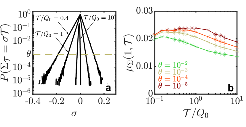
Figure 5: (a) Experimental distributions of the entropy production $P(\Sigma_{\cal T}=\sigma{\cal T})$ for $\tau=8.75$ and $\mathcal{T}/Q_{0}=(0.4,1,10)$. The horizontal dashed line indicates the threshold $\theta$ (here fixed at $10^{-3}$). (b) Estimates of $\mu_{\Sigma}(1,{\cal T})$ versus time for different thresholds. Solid lines are a guide to the eye. The plateau disappears as $\theta$ is increased from $10^{-5}$ to $10^{-2}$.

Consider for instance the data for $\tau=8.75$ in Fig. 4d which shows a plateau around $\mu_{\Sigma}(1,{\cal T})\approx 0.024$ for $\theta=10^{-5}$. As seen in Fig. 5b, this plateau shortens and eventually disappears as $\theta$ increases from $10^{-5}$ to $10^{-2}$, and fewer events contributing to the tails of $P(\Sigma_{{\cal T}})$ are taken into account. This behavior strongly suggests that the decrease of $\mu_{\Sigma}(1,{\cal T})$ displayed in Figs. 4c,d is a statistical artifact that would disappear if all rare events were properly sampled (a similar problem occurs with the heat ${\cal Q}_{\cal T}$ in regime I, and the exact fluctuation relation $\langle e^{-\beta{\cal Q}_{\cal T}}\rangle=e^{-{\cal T}/Q_{0}}$ cannot be verified for ${\cal T}/Q_{0}\gtrsim 2$ even with $5.10^{6}$ trajectories [23]). To estimate $\mu_{\Sigma}(1)$, we thus only consider the (reliable) ascending part of $\mu_{\Sigma}(1,{\cal T})$, using the same fit as before (a check of this procedure in presented in the Supplemental Material [23]). This yields very good agreement with the theoretical expression of $\dot{S}_{J}$ for all delays (Fig. 4e), from which we conclude that the conjecture for the asymptotic fluctuation relation (1) is supported by experiments in regime II as well.

Conclusion. We have experimentally demonstrated the hidden role played by the acausality of the backward process associated with a non-Markovian feedback control. Even though the time-reversed dynamics is not physically realizable, it provides the proper tools (such as the acausal Jacobian or the acausal temperatures) to elucidate the nonequilibrium fluctuations of thermodynamic observables. The verification of these results has required a careful statistical analysis of the asymptotic properties of the exponential average of work and entropy production, including their (nonexponential) prefactors, in order to obtain detailed information about the rare fluctuations of these observables. Our study opens up the exciting possibility of exploring complex behaviors that are not easily amenable to theoretical analysis, for instance those induced by non-linearities in the observables or in the measurement and feedback protocol [37].

Supplementary Information - Non-Markovian feedback control and acausality: an experimental study

Supplemental Material: Non-Markovian feedback control and acausality: an experimental study Maxime Debiossac Martin Luc Rosinberg Eric Lutz Nikolai Kiesel

I Expression of the stochastic entropy production $\Sigma_{{\cal T}}$

As mentioned in the main text, the time-integrated observable $\Sigma_{{\cal T}}$ would be interpreted as the total trajectory-dependent entropy production by an observer unaware of the existence of the feedback loop [1]. According to Ref. [2], this quantity is defined as

$$\Sigma_{{\cal T}} =\Sigma_{\cal T}^{m}+\Sigma_{\cal T}^{sys}\ ,$$ (S1)

where $\Sigma_{\cal T}^{m}=\beta{\cal Q}_{\cal T}$ is the change in the entropy of the medium and $\Sigma_{\cal T}^{sys}=\ln p(x_{0},v_{0})/p(x_{{\cal T}},v_{{\cal T}})$ is the change in the Shannon entropy of the system (cf. Eq. (4) in the main text). The heat ${\cal Q}_{\cal T}$ is related to the work ${\cal W}_{\cal T}$ via the first law that expresses the conservation of energy at the microscopic level

$$\beta{\cal Q}_{\cal T}=\beta{\cal W}_{{\cal T}}-\Delta{\cal U}(x_{0},v_{0},x_{\cal T},v_{\cal T})\ ,$$ (S2)

where

$$\Delta{\cal U}(x_{0},v_{0},x_{\cal T},v_{\cal T})=\frac{1}{Q_{0}}[(x_{\cal T}^{2}-x_{0}^{2})+(v_{\cal T}^{2}-v_{0}^{2})]$$ (S3)

is the change in the internal energy of the system after time ${\cal T}$ (here expressed in reduced units). Moreover, since all forces acting on the particle are linear, the stationary distribution $p(x,v)$ is a bivariate Gaussian,

$$p(x,v)\propto e^{{-\frac{1}{2}\left[\frac{x^{2}}{\langle x^{2}\rangle}+\frac{v^{2}}{\langle v^{2}\rangle}\right]}}\ ,$$ (S4)

as was checked experimentally in Ref. [3]. Replacing the mean-square position and the mean-square velocity by the configurational and kinetic temperatures, defined respectively as $T_{x}/T=(2/Q_{0})\langle x^{2}\rangle$ and $T_{v}/T=(2/Q_{0})\langle v^{2}\rangle$ in reduced units, we arrive at

$$\Sigma_{{\cal T}} =\beta{\cal W}_{{\cal T}}+\frac{1}{Q_{0}}\left[\frac{T-T_{x}}{T_{x}}(x^{2}_{{\cal T}}-x_{0}^{2})+\frac{T-T_{v}}{T_{v}}(v^{2}_{{\cal T}}-v_{0}^{2})\right]\ ,$$ (S5)

where $\beta{\cal W}_{{\cal T}}$ is given by Eq. (3) in the main text.

II Bifurcations and multistability

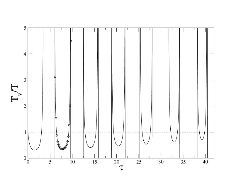
Supplementary Figure S1: Kinetic temperature $T_{v}/T$ of the feedback-controlled oscillator as a function of $\tau$: $T_{v}$ is positive in the regions where a stationary state exists (delimited by the vertical lines). Only the first $7$ stability regions are shown. Experiments (circles) are performed in the second stability region for $5.996<\tau<9.658$. There is no stationary state for a delay $\tau>89.628$.

As shown in Ref. [4], the time-delayed harmonic oscillator obeying Eq. (2) in the main text has a complex dynamical behavior. In particular, for $Q_{0}>\frac{1}{\sqrt{2}}$ and $\frac{1}{Q_{0}}\sqrt{1-\frac{1}{4Q_{0}^{2}}}<|\frac{g}{Q_{0}}|<1$, the oscillator features multistability with a characteristic ”Christmas tree” stability diagram. In the case under study, with $Q_{0}=50.2$ and $g=2.4$, there is an increasing sequence of critical delays ordered as follows,

$$\tau^{*}_{1,1}<\tau^{*}_{1,2}<\tau^{*}_{2,1}<...<\tau^{*}_{14,1}<\tau^{*}_{14,2}<\tau^{*}_{15,1}$$ (S6)

with $\tau^{*}_{1,1}=3.506$, $\tau^{*}_{1,2}=5.996$, $\tau^{*}_{2,1}=9.658$,…, $\tau^{*}_{14,2}=89.521$, $\tau^{*}_{15,1}=89.628$ (in units $\Omega_{0}^{-1}$). As $\tau$ varies from $0$ to $\tau^{*}_{15,1}$, the system switches from stability to instability and back to stability, and is unstable for $\tau>\tau^{*}_{15,1}$. A stationary solution only exists inside the stability domains and the temperatures $T_{x}$ and $T_{v}$ diverges at the boundaries, as illustrated in Fig. S1. The present experimental study is performed in the second stability domain, for $\tau^{*}_{1,2}<\tau<\tau^{*}_{2,1}$.

III Microscopic reversibility and acausal dynamics

For the sake of completeness, we summarize key points of the theoretical analysis performed in Refs. [1, 4, 5].

III.1 Detailed fluctuation relation (or microscopic reversibility)

In the presence of a time-delayed continuous feedback, the fluctuating heat exchanged between the Brownian particle and the thermal bath along a trajectory ${\bf X}$ (see Fig. 1 in the main text) is not odd under time reversal. However, this property is preserved if the time-reversal operation is combined with the change of the delay $\tau\to-\tau$. The heat then obeys the modified detailed fluctuation relation [1, 4]

$$\beta{\cal Q}_{{\cal T}}=\ln\frac{{\cal P}[{\bf X}|{\bf Y}]}{\widetilde{\cal P}[{\bf X}^{\dagger}|{\bf Y}^{\dagger}]}+\ln\frac{\widetilde{\cal J}[{\bf X}]}{{\cal J}}\ ,$$ (S7)

where ${\cal P}[{\bf X}|{\bf Y}]$ is the probability of ${\bf X}$, given the path ${\bf Y}$ in the time interval $[-\tau,0]$, and $\widetilde{\cal P}[{\bf X}^{\dagger}|{\bf Y}^{\dagger}]$ is the probability of ${\bf X}^{\dagger}$, given the time-reversed path ${\bf Y}^{\dagger}$. The “tilde” symbol refers to the “conjugate” acausal dynamics defined by changing $\tau$ into $-\tau$. In general, the corresponding Jacobian $\widetilde{\cal J}[{\bf X}]$ of the transformation $\xi(t)\rightarrow x(t)$ [see Eq. (2) in the main text] is a nontrivial functional of the path, in contrast with the Jacobian ${\cal J}$ of the original causal dynamics. When the system settles in a stable stationary state, one can define the asymptotic rate

$$\dot{\cal S}_{\cal J}=\lim_{{\cal T}\rightarrow\infty}\frac{1}{{\cal T}}\langle\ln\frac{\cal J}{\widetilde{\cal J}[{\bf X}]}\rangle_{\text{st}}\ ,$$ (S8)

which turns out to be an upper bound to the extracted work rate $\dot{\cal W}_{\text{ext}}=-\dot{\cal W}$, i.e.,

$$\beta\langle\dot{\cal W}_{\text{ext}}\rangle_{\text{st}}\leq\dot{\cal S}_{\cal J}\ .$$ (S9)

Note that $\dot{\cal S}_{\cal J}$ generally differs from the so-called ”entropy pumping rate” $\dot{\cal S}_{\text{pump}}$, which is also an upper bound to the extracted work, as tested experimentally in Ref. [3].

The second-law-like inequality (S9) is a consequence of the integral fluctuation theorem $\langle e^{-R_{cg}[{\bf X}]}\rangle=1$ where $R_{cg}[{\bf X}]$ is a rather complicated path-dependent quantity that is not accessible to experiments [4]. However, one has $\dot{\cal R}_{cg}=\beta\dot{\cal Q}+\dot{\cal S}_{\cal J}$ in the long-time limit, where $\dot{\cal R}_{cg}=\lim_{{\cal T}\rightarrow\infty}\frac{1}{\cal T}\langle R_{cg}[{\bf X}]\rangle_{st}$, and the inequality $\langle R_{cg}[{\bf X}]\rangle\geq 0$ implies inequality (S9).

In the case of a linear Langevin dynamics, $\dot{\cal S}_{\cal J}$ can be explicitly expressed in terms of the poles of the acausal response function $\widetilde{\chi}(s)\equiv\chi(s)_{\tau\to-\tau}$ in the complex Laplace plane, where $\chi(s)$ is the standard response function of the oscillator in the Laplace representation [4]. Specifically,

$$\widetilde{\chi}(s)=[s^{2}+\frac{s}{Q_{0}}+1-\frac{g}{Q_{0}}e^{s\tau}]^{-1}$$ (S10)

in reduced units. $\dot{\cal S}_{\cal J}$ is then given by Eq. (160) in Ref. [4].

III.2 Acausal dynamics

Although the acausal dynamics defined by the Langevin equation (here written in reduced units)

$$\ddot{x}_{t}+\frac{1}{Q_{0}}\dot{x}_{t}+x_{t}-\frac{g}{Q_{0}}x_{t+\tau}=\xi_{t},$$ (S11)

is not physically realizable, a stationary solution may still exist, characterized as usual by the fact that the $n$-point probability distributions are invariant under time translation. This also means that the solution must be independent of both the initial condition in the far past and the final condition in the far future, such that

$$x(t)\approx\int_{-\infty}^{+\infty}dt^{\prime}\>\widetilde{\chi}(t-t^{\prime})\xi(t^{\prime})\ ,$$ (S12)

where $\widetilde{\chi}(t)$ is the acausal response function in the time domain. This implies that $\widetilde{\chi}(t)$ decreases sufficiently fast for $t\to\pm\infty$ and in this case $\widetilde{\chi}(t)$ is just the inverse Fourier transform of $\widetilde{\chi}(\omega=is)$ and vice versa (in general, $\widetilde{\chi}(t)$ is defined as the inverse bilateral Laplace transform of the function $\widetilde{\chi}(s)$ defined by Eq. (S10) and it may have no Fourier transform [5]). Concretely, this requires that $\widetilde{\chi}(s)$ has two and only two poles on the l.h.s. of the complex $s$-plane. For the case under study, with the system operating in the second stability region, this occurs for $5.996<\tau<6.854$ and $8.797<\tau<9.658$ (with $\Omega_{0}^{-1}$ as the time unit). The configurational and kinetic temperatures of the “acausal” stationary state (the latter quantity plotted in Fig. 3 of the main text) are then obtained from

$$\frac{\widetilde{T}_{x}}{T} =\frac{2}{Q_{0}}\int_{-\infty}^{+\infty}\frac{d\omega}{2\pi}|\widetilde{\chi}(\omega)|^{2}$$

$$\frac{\widetilde{T}_{v}}{T} =\frac{2}{Q_{0}}\int_{-\infty}^{+\infty}\frac{d\omega}{2\pi}\omega^{2}|\widetilde{\chi}(\omega)|^{2}\ .$$ (S13)

III.3 Asymptotic behavior of $\langle e^{-\Sigma_{{\cal T}}}\rangle$ and $\langle e^{-\beta{\cal W}_{{\cal T}}}\rangle$

When the acausal Langevin Eq. (S11) admits a stationary solution, the theoretical analysis of the asymptotic behavior of the generating functions $Z_{\Sigma}(\lambda,{\cal T})=\langle e^{-\lambda\Sigma_{{\cal T}}}\rangle$ and $Z_{W}(\lambda,{\cal T})=\langle e^{-\lambda\beta{\cal W}_{{\cal T}}}\rangle$ for ${\cal T}\to\infty$ and $\lambda=1$ suggests that $\mu_{W}(1)=\mu_{\Sigma}(1)=\dot{\cal S}_{\cal J}$ [5]. At the same time, the expression of the ratio $g_{W}(1)/g_{\Sigma}(1)$ of the pre-exponential factors (Eq. (4) in the main text) is more an educated guess based on perturbative calculations and on the exact behavior of the system in some limiting cases (e.g., the small-$\tau$ and large-$Q_{0}$ limits).

On the other hand, when the ”acausal” stationary solution does not exist, things are more complicated. However, the explicit result $\mu_{W}(1)=1/Q_{0}$ can be proven when the conjugate dynamics obtained by changing the sign of the friction coefficient in the original Langevin equation (the so-called “hat” dynamics in Ref. [5]) relaxes to a stationary state. This is what occurs for $6.85\lesssim\tau\lesssim 8.80$ (grey region in Fig. 4e of the main text). On the other hand, there is yet no exact theoretical prediction for $\mu_{\Sigma}(1)$, and the main conjecture tested in this work, stating that $\mu_{\Sigma}(1)$ is always equal to $\dot{\cal S}_{\cal J}$, is based on a limited set of simulation results.

III.4 Stationary-state fluctuation theorem

Because of the non-Markovian feedback, the system does not obey a conventional stationary-state fluctuation theorem (SSFT) expressing the symmetry around $0$ of the pdf of an observable at large times, for instance $\lim_{{\cal T}\to\infty}\frac{1}{{\cal T}}\ln[P(\beta{\cal W}_{\cal T}=w{\cal T})/{P(\beta{\cal W}_{\cal T}=-w{\cal T})}]=w$ for the work done by an external force (see e.g. Ref. [6]). However, provided the acausal stationary state exists, this relation is replaced by [5]

$$\lim_{{\cal T}\to\infty}\frac{1}{{\cal T}}\ln\frac{P(\beta{\cal W}=w{\cal T})}{\widetilde{P}(\beta\widetilde{\cal W}=-w{\cal T})}=w+\dot{S}_{\cal J}\ ,$$ (S14)

where $\beta\widetilde{\cal W}_{\cal T}\equiv\beta{\cal W}_{\cal T}|_{\tau\to-\tau}=(2g)/(Q_{0}^{2})\int_{0}^{{\cal T}}dt^{\prime}\>x_{t^{\prime}+\tau}\circ v_{t^{\prime}}$.

A check of this modified SSFT is shown in Fig. S2 for $\tau=6.51$, with $P(\beta{\cal W}_{{\cal T}}=w{\cal T})$ and $\dot{S}_{J}$ obtained from experiments (specifically, $\dot{S}_{J}\approx 0.0045$ from the fit of $\mu_{\Sigma}(1,\mathcal{T})$, which is close to the theoretical value, as can be seen in Fig. 4e of the main text). It is obviously crucial to include this contribution in the SSFT to reach a good agreement. To compute the “acausal” probability $\widetilde{P}(\beta\widetilde{\cal W}=-w{\cal T})$, a large number of stationary trajectories of length ${\cal T}$ generated by Eq. (S11) is needed. Like in Ref. [5], this can done by computing numerically the response function $\widetilde{\chi}(t)$ and then using Eq. (S12) (the case shown in Fig. S2 turns out to be rather challenging because $\widetilde{\chi}(t)$ decreases very slowly with $t$ for $t>0$). Another method is to solve the acausal Langevin equation (S11) iteratively as

$$\dot{v}_{t}^{(n)}=-\frac{1}{Q_{0}}v_{t}^{(n)}-x_{t}^{(n)}+\frac{g}{Q_{0}}x_{t+\tau}^{(n-1)}+\xi_{t}\ ,$$ (S15)

starting for some initial trajectory $\{x_{t}^{(0)}\}$ of length ${\cal T}^{(0)}\gg{\cal T}$ and reducing the length of the trajectory by $\tau$ at each iteration. This procedure circumvents the obstacle of non-causality since an entire time sequence is available from the previous iteration. This is somewhat similar to the non-causal learning algorithm used in iterative learning [7]. However, convergence of the procedure is not guaranteed and requires to properly choose the initial trajectory. Of course, this cannot be done experimentally.

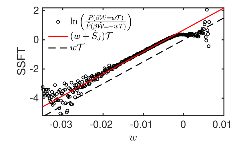
Supplementary Figure S2: Verification of the modified stationary-state fluctuation theorem (SSFT) $\ln[P(\beta{\cal W}=w{\cal T})/\widetilde{P}(\beta\widetilde{\cal W}=-w{\cal T})]\sim(w+\dot{S}_{J}){\cal T}$ for $\tau=6.51$ ($\Omega_{0}^{-1}$ is the time unit). The trajectory length is ${\cal T}=3Q_{0}$. The “acausal” probability $\widetilde{P}(\beta\widetilde{\cal{W}}=-w{\cal T})$ is obtained as explained in the text.

IV Method and statistical analysis

IV.1 Block averaging and rare events

The estimates of the scaled cumulant generating functions (SCGF) $\mu_{W}(1)$ and $\mu_{\Sigma}(1)$ are obtained by using a block averaging approach. In the context of large deviation theory, this method is well-suited for integrated observables of continuous-time random processes [8, 9, 10]. We thus divide the recorded trajectory of length ${\cal T}_{tot}=1000$ s into $N$ blocks (i.e., trajectories) of length ${\cal T}$, separated one from another by $\Delta{\cal T}$. Hence ${\cal T}_{tot}=N{\cal T}+(N-1)\Delta{\cal T}$. To ensure that $x(t)$ and $x(t-\tau)$ belong to the same block, $\Delta{\cal T}$ is much larger than the largest value of $\tau$ considered in our experiments. Specifically, $\Delta{\cal T}\approx 0.053$ ms (i.e. $\Delta{\cal T}=2Q_{0}=100.4$ in reduced units whereas $\tau_{max}\approx 9.50$). The observables are then computed in each block. Consider for instance the work. The estimator of $Z_{W}(1,{\cal T})=\langle e^{-\beta{\cal W}_{{\cal T}}}\rangle$ is given by

$$\hat{Z}_{W}(1,N,{\cal T})=\frac{1}{N}\sum_{j=1}^{N}e^{-\beta{\cal W}_{{\cal T}}^{(j)}}\ ,$$ (S16)

where $\beta W_{{\cal T}}^{(j)}=\frac{2g}{Q_{0}^{2}}\int_{t_{j}}^{tj+{\cal T}}dt\>x_{t-\tau}\circ v_{t}$ and $t_{j}=(j-1)({\cal T}+\Delta{\cal T})$ is the initial time of block $j$. Since time is discretized, the velocity is computed as $v_{i}=(x_{i+1}-x_{i})/\Delta t$ (with $\Delta t=0.2\mu$s), and a spline interpolation of the time series is used to precisely pinpoint the position of the particle at time $t-\tau$.

The estimator of $\mu_{W}(1,{\cal T})\equiv(1/{\cal T})\ln Z_{W}(1,{\cal T})$ is then

$$\hat{\mu}_{W}(1,N,{\cal T})=\frac{1}{\cal T}\ln\hat{Z}_{W}(1,N,{\cal T})\ .$$ (S17)

In principle, two limits must be successively taken to obtain the SCGF: first $\lim_{N\to\infty}\hat{\mu}_{W}(1,N,{\cal T})=\mu_{W}(1,{\cal T})$, and then $\lim_{{\cal T}\to\infty}\mu_{W}(1,{\cal T})=\mu_{W}(1)$. In practice, however, one is constrained by the fixed length ${\cal T}_{tot}$ of the recorded time series, and one faces a trade-off in the choice of ${\cal T}$ and $N$ [10]. For instance, one has ${\cal T}\leq{\cal T}_{\max}\approx 0.15$ ms with $N=5.10^{6}$ blocks and ${\cal T}\leq{\cal T}_{\max}\approx 0.29$ ms with $N=3.10^{6}$ (respectively ${\cal T}_{\max}/Q_{0}\approx 5.45$ and ${\cal T}_{\max}/Q_{0}\approx 10.42$ in reduced units). In fact, Figs. 4 and 5 in the main text show that the rare events which make $\langle e^{-\Sigma_{\cal T}}\rangle$ different from $\langle e^{-{\cal W}_{\cal T}}\rangle$ in regime II come into play for ${\cal T}$ significantly smaller than ${\cal T}_{\max}$.

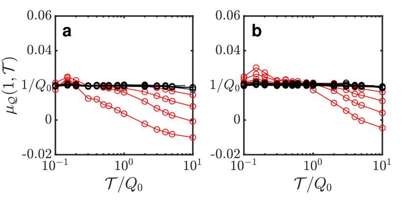
Supplementary Figure S3: Estimates of $\mu_{Q}(1,{\cal T})$ as a function of the observation time ${\cal T}$ for delays $6.13\leq\tau\leq 7.82$ (a) and $8.00\leq\tau\leq 9.50$ (b). The values of the delay $\tau$ and the color of the symbols are the same as in Fig. 4 of the main text.

Remarkably, the dissipated heat ${\cal Q}_{\cal T}$ displays a similar behavior in regime I. The crucial difference with the entropy production is that ${\cal Q}_{\cal T}$ satisfies the integral fluctuation theorem (IFT) $\langle e^{-\beta{\cal Q}_{\cal T}}\rangle=e^{-(\Gamma/m){\cal T}}$ at all times (a universal result for underdamped Langevin dynamics [11]). Hence, one should observe that $\mu_{Q}(1,{\cal T})=1/Q_{0}$ in reduced units. However, as shown in Fig. S3, this is only observed in regime II (black symbols in the figure), that is, when the ”hat” dynamics [5] obtained by changing the sign of the friction coefficient relaxes to a stationary state. In regime I (red symbols), the estimated values of $\mu_{Q}(1,{\cal T})$ exhibit a spurious behavior as a function of ${\cal T}$ which resembles the one found for $\mu_{\Sigma}(1,{\cal T})$.

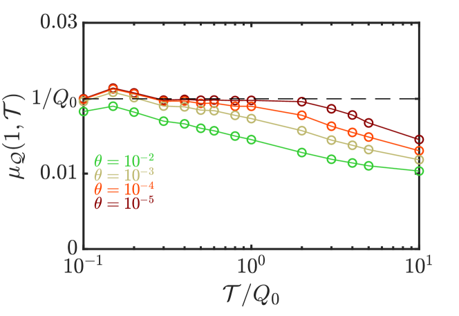
Supplementary Figure S4: Estimates of $\mu_{Q}(1,{\cal T})$ versus time for $\tau=6.70$ and different thresholds. Dashed lines are a guide to the eye. One should observe $\mu_{Q}(1,{\cal T})=1/Q_{0}$ but the plateau disappears as $\theta$ is increased from $10^{-5}$ to $10^{-2}$.

Figure S4 (for $\tau=6.70$) is similar to Fig. 5b in the main text and clearly shows that the correct IFT is progressively recovered (at least for ${\cal T}/Q_{0}\lesssim 2$) as the threshold $\theta$ is decreased and more events contributing to the tails of the pdf of the heat are included in the calculation of the exponential average. This further supports our claim that the fall-off of $\mu_{\Sigma}(1,{\cal T})$ for ${\cal T}/Q_{0}\gtrsim 1$ is also spurious.

IV.2 Extrapolation and errors

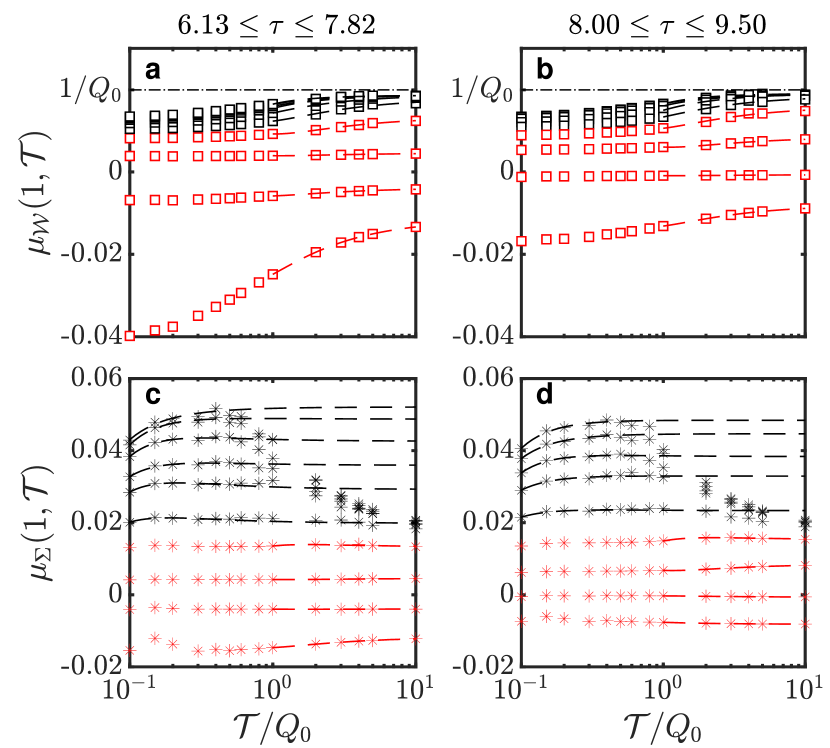
Supplementary Figure S5: Same as Figs. 4a-d in the main text with the dashed lines representing the fits of the finite-time values that are used to extract the asymptotic scaled cumulant generating functions and the pre-exponential factors in regime I.

The infinite-time limit of the estimators of the SCGF’s are extracted from the finite-time results using a fit of the form $a+b/{\cal T}+c/{\cal T}^{2}$. We note that this type of $1/{\cal T}$ scaling has also been used to evaluate large-deviation functions obtained by a population dynamics algorithm [12]. This leads to the fits represented by the dashed lines in Fig. S5. We recall that the fits in regime I (red dashed lines) are done in the range $1\leq{\cal T}/Q_{0}\leq 10$ for both the work and the entropy production. This allows us to obtain a sensible estimation of the pre-exponentials factors $g_{W}(1)$ and $g_{\Sigma}(1)$ in addition to the asymptotic SCGFs. On the other hand, the values of $\mu_{\Sigma}(1,{\cal T})$ in regime II (black dashed lines) are fitted for ${\cal T}/Q_{0}\lesssim 0.4$ only since the statistics of the rare events is clearly deficient at larger times. As shown in Fig. S6 (which corresponds to Fig. 4e in the main text), the fit of $\mu_{\Sigma}(1,{\cal T})$ in regime I can also be done for ${\cal T}/Q_{0}\lesssim 0.4$ without significantly changing the extrapolated values of the SCGF. However, one can no longer extract a reliable value of the pre-exponential factor $g_{\Sigma}(1)$ from the $1/{\cal T}$ correction.

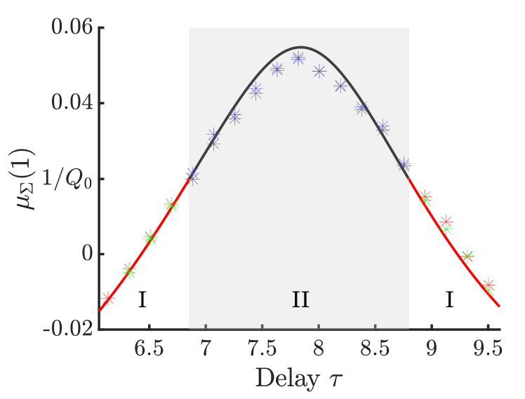
Supplementary Figure S6: Comparison of the SCGF $\mu_{\Sigma}(1)$ using different analysis methods. In regime I, red stars results from a fit performed in the interval $1\leq\mathcal{T}/Q_{0}\leq 10$, while green stars is for a fit in the interval $0.1\lesssim{\cal T}/Q_{0}\lesssim 0.4$. Note that, for $\tau=6.13$ (first delay), this latter fit cannot be done because of the non-monotonic behavior of $\mu_{\Sigma}(1,{\cal T})$ at small times. In regime II, black stars are obtained with a fit in the interval $0.1\lesssim{\cal T}/Q_{0}\lesssim 0.4$ and are compared with the values given by the maximum of $\mu_{\Sigma}(1,{\cal T})$ (blue stars).

It would be desirable to provide confidence intervals for $\mu_{W}(1,{\cal T})$, $\mu_{\Sigma}(1,{\cal T})$, and eventually for the SCGFs. This requires to estimate the statistical and systematic errors due to the finite value of $N$, that is the variance and the bias of the estimators (see e.g., Refs.[13, 14, 15]), in addition to the experimental uncertainties in the values of the damping rate and the feedback gain mentioned in the main text. However, this is a very challenging task in the present case because the probability distributions of the observables are not Gaussian. In particular, $P(\Sigma_{\cal T})$ has an exponential tail on the left-hand side, which in the large-deviation regime is associated with the presence of poles in the pre-exponential factor [5]. The main problem is that the distribution of $e^{-\Sigma_{\cal T}}$ may not have a finite second moment, so that the estimator may not converge asymptotically to a Gaussian distribution around the mean [9]. This crucially depends on the value of $\tau$, as illustrated in Fig. S7 for ${\cal T}/Q_{0}=1$ and two different values of $\tau$ (respectively in regime I and II). The statistical distributions have been obtained by grouping the $N=5.10^{6}$ trajectories into $N_{b}=1000$ blocks of size $n=N/N_{b}=5000$, and computing the average $\langle\hat{\mu}_{\Sigma}(1,N,{\cal T})\rangle_{b}=(1/{\cal T})\langle\ln\hat{Z}_{\Sigma}(1,N,{\cal T})\rangle_{b}$ in each block. For $\tau=6.32$, the variance of $P(e^{-\Sigma_{\cal T}})$ is finite, and it can be seen that the distribution of $\langle\hat{\mu}_{\Sigma}(1,N,{\cal T})\rangle_{b}$ is reasonably Gaussian. On the other hand, the variance diverges for $\tau=7.82$, and the distribution of $\langle\hat{\mu}_{\Sigma}(1,N,{\cal T})\rangle_{b}$ is strongly asymmetric with a long tail on the right-hand side. In the first case, the statistical error is the dominant source of noise [14, 15], but the final error on $\hat{\mu}_{\Sigma}(1,{\cal T})$ turns out to be very small (of the order $10^{-6}$, which is too small to be visible in Fig. 4 in the main text). In the second case, it is very likely that the bias due to the undersampling of the rare events associated with the temporal boundary term is dominant but, unfortunately, a reliable estimate cannot be obtained. This difficult issue is left for future investigations.

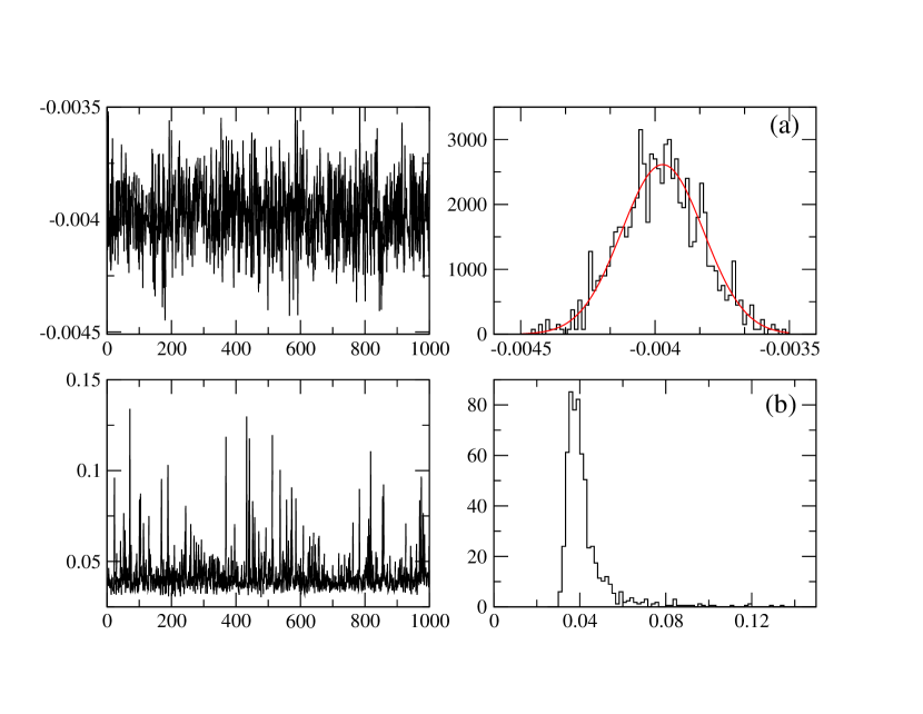
Supplementary Figure S7: Values of $\langle\hat{\mu}_{\Sigma}(1,N,{\cal T})\rangle_{b}$ calculated in $1000$ blocks of size $n=5000$ and the corresponding statistical distributions for ${\cal T}/Q_{0}=1$, $\tau=6.32$ (a) and $\tau=7.82$ (b). The solid red line in panel (a) is the best fit by a Gaussian distribution. The distribution is non-Gaussian in panel (b).

References

- [1] T. Munakata and M. L. Rosinberg, Entropy Production and Fluctuation Theorems for Langevin Processes under Continuous Non-Markovian Feedback Control, Phys. Rev. Lett. 112, 180601 (2014).
- [2] U. Seifert, Entropy production along a stochastic trajectory and an integral fluctuation theorem, Phys. Rev. Lett. 95, 040602 (2005).
- [3] M. Debiossac, D. Grass, J. J. Alonso, E. Lutz, and N. Kiesel, Thermodynamics of continuous non-Markovian feedback control, Nature Commun. 11, 1360 (2020).
- [4] M.L. Rosinberg, T. Munakata, and G. Tarjus, Stochastic thermodynamics of Langevin systems under time-delayed feedback control: Second-law-like inequalities, Phys. Rev. E 91, 042114 (2015).
- [5] M.L. Rosinberg, G. Tarjus, and T. Munakata, Stochastic thermodynamics of Langevin systems under time-delayed feedback control. II. Nonequilibrium steady-state fluctuations, Phys. Rev. E 95, 022123 (2017).
- [6] S. Ciliberto, Experiments in Stochastic Thermodynamics: Short History and Perspectives, Phys. Rev. X 7, 021051 (2017).
- [7] D. A. Bristow, M. Tharayil, and A. G. Alleyne, A survey of iterative learning control, IEEE Control Systems Magazine 26, 96 (2006).
- [8] K. Duffy and A. P. Metcalfe, The large deviations of estimating rate functions, J. Appl. Prob. 42, 267 (2005).
- [9] C. M. Rohwer, F. Angeletti, and H. Touchette, Convergence of large-deviation estimators, Phys. Rev. E 92, 052104 (2015).
- [10] F. Ragone and F. Bouchet, Computation of extremes values of time averaged observables in climate models with large deviation techniques, J. Stat. Phys. 179, 1637 (2020).
- [11] M. L. Rosinberg, G. Tarjus, and T. Munakata, Heat fluctuations for underdamped Langevin dynamics, Eur. Phys. Lett. 113, 10007 (2016).
- [12] E. G. Hidalgo, T. Nemoto, and V. Lecomte, Finite-time and finite-size scalings in the evaluation of large-deviation functions: Numerical approach in continuous time, Phys. Rev. E 95, 062134 (2017).
- [13] D. M. Zuckerman and T. B. Woolf, Theory of a Systematic Computational Error in Free Energy Differences, Phys. Rev. Lett. 89, 180602 (2002).
- [14] J. Gore, F. Ritort, and C. Bustamante, Bias and error in estimates of equilibrium free-energy differences from nonequilibrium measurements, Proc. Natl. Acad. Sci. U.S.A. 100, 12564 (2003).
- [15] A. Pohorille, C. Jarzynski, and C. Chipot, Good Practices in Free-Energy Calculations, J. Phys. Chem. B, 114, 10235 (2010).