Passage of test particles through oscillating spherically-symmetric dark matter configurations

Abstract

Applying the perturbative approach to geodesic equations, we study motion of the test particles in time-dependent spherically symmetric spacetimes created by oscillating dark matter. Assuming the weakness of the gravitational field, we derive general formulas that describe infinite trajectories of the test particles and determine the total deflection angle in the leading order approximation. The obtained formulas are valid for both time-dependent and static matter configurations. Using these results, we calculate the deflection angle of a test particle passing through a spherically symmetric oscillating distribution of a self-gravitating scalar field with a logarithmic potential. It turned out that, in a wide range of amplitudes, oscillations in the deflection angle are sinusoidal and become small for ultrarelativistic particles.

I Introduction

Despite the great efforts of theorists and significant advances in technologies and methods of observation, the nature of dark matter (DM) remains unknown. The standard $\Lambda$CDM model, which explains observational data well at cosmological scales, faces serious problems at galactic and subgalactic scales (see, e.g., Primack ). One of the most cited possibilities to overcome these difficulties is to assume that DM consists of ultra-light bosonic particles with masses in the $10^{-23}-10^{-21}$ eV range, e.g., axions Marsh , which are in a coherent state described by a classical scalar field Turner ; Seidel1 ; Seidel2 ; Kolb ; Lee ; Peebles ; Hu ; Matos ; Magana ; Hui . In the early Universe, the primordial fluctuations of this field are stretched by inflation, this evolution resulting in the formation of a uniform scalar background oscillating near the minimum of the effective potential. These oscillations are unstable Khlopov . In the case of the quadratic potential, the oscillating background behaves as a dust-like matter, so that some kind of the Jeans instability can occur Hu . In addition, in the case of a self-interacting scalar field, another instability mechanism comes into play. This mechanism is based on parametric resonance between the oscillating background and perturbations and works on both cosmological and astrophysical scales Kofman ; Koutvitsky0 ; Amin ; Zhang ; Lozanov ; Koutvitsky1 ; Fukunaga ; Arvanitaki . At the nonlinear stage this leads to formation of quasi-stable oscillating lumps, oscillons (pulsons), (see Olle for a recent review). Under the influence of gravity, after the completion of some relaxation processes, these lumps turn into long-lived self-gravitating oscillating objects, oscillatons (gravipulsons) Urena ; Fodor ; Koutvitsky2 , separated from the Hubble flow. The latter means that the dynamics of an individual oscillaton should be determined by the self-consistent system of Einstein-Klein-Gordon equations. Note that oscillatons can arise from rather arbitrary localized initial conditions due to the gravitational cooling process Seidel1 ; Seidel2 ; Guzman . This process is very similar to that which occurs in the integrable systems, when an initial state decays into solitons and outgoing waves.

On galactic and subgalactic scales, oscillaton solutions can describe various localized objects, from oscillating soliton stars to oscillating DM halos, depending on the assumed mass of the scalar field. Oscillations of the scalar field in these objects cause oscillations of the gravitational potential, which can be detected by their effect on the motion of photons and test bodies. In particular, as shown in Khmelnitsky , the gravitational time delay for a photon passing through an oscillating halo should cause small periodic fluctuations in the observed timing array of the pulsar located inside the halo. Although the predicted effect is very small, the authors believe it can be detected in the next generation of pulsar timing observations. In paper Aoki , it was proposed to use the laser interferometers for detecting the axion wind caused by passage of the Earth through DM. The gravitational field oscillations, produced by the oscillating DM, look like gravitational waves to an observer on Earth and would be detected in future laser interferometer experiments. An approach based on the observations of binary pulsars was discussed in Blas ; Rozner to probe of ultralight axion DM. It was shown that oscillations of DM resonantly perturb the orbits of the binary pulsars thus leading to secular variations in their orbital period. Also, in the context of oscillating DM, in Refs. Becerril ; Boskovic the orbital motion of test bodies in spherically symmetric time-periodic spacetimes was studied numerically. In particular, it was demonstrated in Boskovic that the orbital resonances may occur in motion of stars in oscillating spherically symmetric halos. In addition, in Refs. Boskovic ; Koutvitsky3 it was shown that spectroscopic emission lines from stars in such halos exhibit characteristic, periodic modulation patterns due to variations in the gravitational frequency shift. These results show that the motion of photons and test bodies may carry distinguishable observational imprints of the oscillating DM.

Recently, in the above context, we studied the deflection of photons in time-periodic spherically symmetric gravitational fields Koutvitsky4 . Using the geodesic method and the perturbative approach, we have shown that the deflection angle of a light ray in general undergoes periodic variations when passing through such fields. In observations, this can lead to additional variations of intensity of images when lensing the distant sources. In the present paper, following the approach developed in Koutvitsky4 , we study the deflection of massive particles.

Our paper is organized as follows. In Sec. II, assuming the weakness of the gravitational field, we use the perturbative approach to describe the infinite trajectories of massive particles in nonstatic spherically symmetric spacetimes. In particular, we obtain general formulas which determine the deflection angle of a massive particle in the leading order approximation. In Sec. III, we apply these formulas to calculate the deflection angle of a massive test particle passing through an oscillating dark matter configuration formed by a real scalar field with a logarithmic self-interaction. Discussion and concluding remarks can be found in Sec. IV.

II Infinite trajectories of test particles in nonstatic
spherically symmetric spacetimes

Let us consider a spherically symmetric nonstatic metric of the form

$$ds^{2}=B(t,r)\,dt^{2}-A(t,r)\,dr^{2}-r^{2}(d\vartheta^{2}+\sin^{2}\vartheta\,d\varphi^{2}),$$ (1)

where $A(t,r)$ and $B(t,r)$ tend to unity as $r\rightarrow\infty$. For the trajectories lying in the plane $\vartheta=\pi/2$, the geodesic equation reduces to the system

$$\frac{d}{ds}\ln\left(B\frac{dt}{ds}\right)=\frac{\dot{B}}{2B}\frac{dt}{ds}-\frac{\dot{A}}{2B}\left(\frac{dr}{ds}\right)^{2}\left(\frac{dt}{ds}\right)^{-1},$$ (2)

$$\frac{d^{2}r}{ds^{2}}+\frac{B^{\prime}}{2A}\left(\frac{dt}{ds}\right)^{2}+\frac{\dot{A}}{A}\frac{dt}{ds}\frac{dr}{ds}+\frac{A^{\prime}}{2A}\left(\frac{dr}{ds}\right)^{2}-\frac{r}{A}\left(\frac{d\varphi}{ds}\right)^{2}=0,$$ (3)

$$\frac{d^{2}\varphi}{ds^{2}}+\frac{2}{r}\frac{dr}{ds}\frac{d\varphi}{ds}=0,$$ (4)

where $(\dot{\phantom{.}})=\partial/\partial t$, $\left({}^{\prime}\right)=\partial/\partial r$. From Eqs. (4) and (1) it follows that

$$\frac{d\varphi}{ds}=\frac{J}{r^{2}},$$ (5)

$$A\left(\frac{dr}{ds}\right)^{2}-B\left(\frac{dt}{ds}\right)^{2}+\frac{{J}^{2}}{r^{2}}+1=0,$$ (6)

where ${J}=const$. It is easy to see that for a particle (e.g., of unit mass) coming from a distant point with an initial velocity $v$ and an impact parameter $b$

$${J}=bv\,{E},\quad{E}=\left(1-v^{2}\right)^{-1/2},$$ (7)

so that ${J}$ is the particle’s angular momentum, ${E}$ is the initial kinetic energy.

Let us assume that the gravitational field is time-dependent and weak everywhere on the particle trajectory, i.e.,

$$A=1-2\psi+O(\varkappa^{2}),\quad B=1+2\chi+O(\varkappa^{2}),$$ (8)

where $\psi(t,r)$ and $\chi(t,r)$ are small functions of order $\varkappa$, $\varkappa\ll 1$ being a dimensionless small parameter proportional to the gravitational constant $G$.

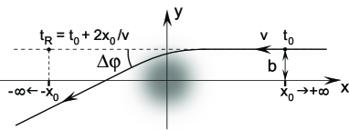
Figure 1: Passage of the test particle through the gravitating mass

Now suppose that in the $xy$ plane at a distant point $x=x_{0}$, $y=b$ at a moment $t_{0}$, a particle begins to move with an initial velocity $v$ parallel to the $x$ axis in the direction of the gravitating mass (see Fig. 1). If the gravitating mass were absent, the particle would move along the straight line,

$$x=x_{0}+v(t_{0}-t),\quad y=b,$$ (9)

and be registered at the moment $t_{R}=t_{0}+2x_{0}/v$ at the distant point $x=-x_{0}$, $y=b$. On this line

$$r(t)=\sqrt{x^{2}(t)+b^{2}},\quad dt/ds=E.$$ (10)

With the gravitating mass, the particle will move along a deflected trajectory with the current radial coordinate

$$r(t)=\left(1+\eta(t)\right)\sqrt{x^{2}(t)+b^{2}},$$ (11)

where, as before,

$$x=v(t_{R}-t)-x_{0},$$ (12)

and $\eta(t)$ is a small function of order $\varkappa$. On this trajectory, the dependence $t(s)$ is determined by Eq. (2), where we set

$$B\frac{dt}{ds}=E\left(1+\zeta(t)\right),$$ (13)

with a small function $\zeta(t)\sim\varkappa$. Then, with the required accuracy, from Eq. (2) we obtain

$$\frac{d\zeta}{dt}=\dot{\chi}(t,r)+v^{2}\dot{\psi}(t,r)\left(1-\frac{b^{2}}{r^{2}}\right).$$ (14)

To get the equation for $\eta$, we proceed from Eq. (6), where $dr/ds=(dr/dt)\left(dt/ds\right)$, and $r$ is now given by Eq. (11). Calculating $dr/dt$ and using Eqs. (7), (8), and (13), in the first order in $\varkappa$ we arrive at the equation

$$vx(x^{2}+b^{2})\frac{d\eta}{dt}-v^{2}(x^{2}-b^{2})\eta+v^{2}x^{2}\psi(t,r)+$$

$$\left[\left(2v^{2}\!-\!1\right)x^{2}\!-\!b^{2}\right]\!\chi(t,r)+\left[\left(1\!-\!v^{2}\right)x^{2}\!+\!b^{2}\right]\zeta(t)=0.\qquad$$ (15)

Further, from Eq. (5), using Eqs. (7), (8), (11), and (13), we find

$$\frac{d\varphi}{dt}=\frac{vb}{x^{2}+b^{2}}\left[1+\left(2\chi-\zeta-2\eta\right)\right].$$ (16)

Since in Eqs. (14)-(16) $t=t_{R}-\left(x+x_{0}\right)/v$ and $r=\sqrt{x^{2}+b^{2}}$, we can integrate over $x$ instead of $t$, setting $dx=-v\,dt$. As a result, we obtain

$$\zeta=\frac{1}{v}\int_{x}^{x_{0}}\left[\dot{\chi}(t,r)+v^{2}\dot{\psi}(t,r)\left(1-\frac{b^{2}}{r^{2}}\right)\right]\;dx,$$ (17)

$$\eta=\frac{x}{v^{2}\left(x^{2}+b^{2}\right)}\times$$

$$\left\{\!\int\bigg{[}v^{2}x^{2}\psi(t,r)+\left(\left(2v^{2}\!-\!1\right)x^{2}-b^{2}\right)\chi(t,r)+\left(\left(1\!-\!v^{2}\right)x^{2}+b^{2}\right)\zeta(t)\bigg{]}\frac{dx}{x^{2}}+const\right\},$$ (18)

$$\varphi=\pi/2-\,\mathrm{arctg}\,(x/b)+b\int_{x}^{x_{0}}\frac{2\chi-\zeta-2\eta}{x^{2}+b^{2}}\,dx.$$ (19)

These equations completely describe, in the leading order, the trajectory of the test particle that was emitted at a distant point with the coordinates $(x_{0},b)$ and registered by a distant observer at the moment $t_{R}$. The $constant$ in Eq. (18) can be found from the condition $\eta(x_{0})=0$, but it does not affect the complete change of $\varphi$ for the particle coming from infinity and going to infinity. Indeed, taking $x=-x_{0}$ and setting $x_{0}\rightarrow\infty$, we find $\varphi=\pi+\Delta\varphi$, where

$$\Delta\varphi=b\int_{-\infty}^{\infty}\frac{2\chi-\zeta-2\eta}{x^{2}+b^{2}}\,dx$$ (20)

is the deflection angle.

The obtained formulas are valid not only for time-dependent metrics, but also for the static ones. In the latter case one should put $\zeta=0$ in accordance with Eq. (17). Consider, for example, the Schwarzschild metric. Assuming $r_{g}/b=\varkappa\ll 1$, where $r_{g}=2GM$ is the gravitational radius, we have

$$\psi=\chi=-\varkappa\frac{b}{2r}.$$ (21)

Then, formula (18) gives

$$\eta=-\varkappa\,\frac{bx}{2v^{2}(x^{2}+b^{2})}\left[\frac{\sqrt{x^{2}+b^{2}}}{x}+\left(3v^{2}-1\right)\,\mathrm{arsh}\,\frac{x}{b}+const\right]\!.$$ (22)

Substituting (21) and (22) into (20) and integrating, we reproduce the well-known result,

$$\Delta\varphi=\frac{2GM}{bv^{2}}\left(1+v^{2}\right)+O((r_{g}/b)^{2}).$$ (23)

Note that this formula is only valid for $v^{2}\gg\varkappa=2GM/b$.

In the case of a time-dependent metric, the deflection angle for a large fixed $x_{0}$ will generally depend on the particle emission time $t_{0}$ or, equivalently, on the observation time $t_{R}=t_{0}+2x_{0}/v$, since when integrating in (17)-(20) we substitute $t=t_{R}-\left(x+x_{0}\right)/v$ into the potentials $\psi(t,r)$ and $\chi(t,r)$. For time-periodic potentials (with a certain period $T_{g}$), we can ignore $x_{0}$ in the integrands by setting for convenience $x_{0}=nT_{g}v$, where $n$ is a large integer. Then the moment $t_{R}$ will determine in which phase of the oscillations of the gravitational field the particle passed through the matter distribution and, consequently, at what angle it deflected as a result of this.

In the next section, we calculate the deflection angle of the test particle passing through the oscillating distribution of a real scalar field with a logarithmic self–interaction.

III Deflection of the test particle by a time-periodic
spherically symmetric scalar field

As a deflecting matter, we consider the self-gravitating real scalar field with the potential

$$U(\phi)=\frac{m^{2}}{2}\phi^{2}\left(1-\ln\frac{\phi^{2}}{\sigma^{2}}\right),$$ (24)

where $\sigma$ is the characteristic magnitude of the field, $m$ is the mass (in units $\hbar=c=1)$. Originally, such potentials were considered in quantum field theory Rosen ; Birula . Also, when taking into account quantum corrections, they naturally appear in inflationary cosmology Linde ; Barrow , as well as in some supersymmetric extensions of the Standard Model Enqvist . It is remarkable that potential (24) admits exact solutions of the Klein-Gordon equation in the form of multidimensional localized time-periodic field configurations, the pulsons (oscillons) Marques ; Bogolubsky ; Maslov . The corresponding solution of the Einstein–Klein–Gordon system was found in paper Koutvitsky2 by the Krylov-Bogoliubov method. This solution describes a self-gravitating field lump of an almost Gaussian shape that pulsates in time. In the weak field approximation, the corresponding metric functions $A(t,r)$ and $B(t,r)$ can be written as (8), where

$$\psi(t,r)\!=\frac{\varkappa}{2}\!\left[V_{\max}\!\left(1\!-\!\frac{\sqrt{\pi}\,\mathrm{erf}\,\rho}{2\rho}e^{\rho^{2}}\!\right)\!+\!a^{2}\rho^{2}\right]\!e^{3-\rho^{2}},\\$$ (25)

$$\chi(t,r)\!=\!-\frac{\varkappa}{2}\!\left[V_{\max}\!\left(1\!+\!\frac{\sqrt{\pi}\,\mathrm{erf}\,\rho}{2\rho}e^{\rho^{2}}\!\right)\!+\!a^{2}\ln a^{2}\right]\!e^{3-\rho^{2}},$$ (26)

$\tau=mt$, $\rho=mr$, $\varkappa=4\pi G\sigma^{2}\ll 1$ ($G$ is the gravitational constant). The function $a(\theta(\tau))$ oscillates in the range $-a_{\max}\leqslant a(\theta)\leqslant a_{\max}$ in the local minimum of the potential $V(a)$,

$$a_{\theta\theta} = -dV/da,$$ (27)

$$V(a) = (a^{2}/2)\left(1-\ln a^{2}\right),$$ (28)

where $V_{\max}=V(a_{\max})$, $\theta_{\tau}=1+\varkappa\Omega+O(\varkappa^{2})$, and the constant $\varkappa\Omega$ is the frequency correction due to gravitational effects (see Ref. Koutvitsky2 for details). The period (in $\theta$) of these oscillations is given by

$$T=4\int_{0}^{1}\left[(1-\ln a_{\max}^{2})(1\!-\!z^{2})+z^{2}\ln z^{2}\right]^{-1/2}dz.$$ (29)

The dependence of the period on $a_{\max}^{2}$ is shown in Fig. 2. With $a_{\max}^{2}\ll 1$ it can be approximated by $T\approx 2\pi\left(1-\ln a_{\max}^{2}\right)^{-1/2}$.

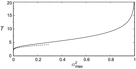
Figure 2: Field oscillation period versus $a^{2}_{max}$ (solid line) and its approximation for small amplitudes (dashed line)

The energy density of the field lump we are considering is concentrated on the characteristic scale $r\sim m^{-1}$. As seen from Eqs. (25) and (26), at large distances from the lump the gravitational field turns into the static Schwarzschild field (21) with the mass $M=\left(e\sqrt{\pi}\right)^{3}\sigma^{2}m^{-1}V_{\max}$, in accordance with the Birkhoff theorem (see, e.g., Weinberg ). However, inside the lump the gravitational field oscillates with the period $T_{g}=[2m(1+\varkappa\Omega)]^{-1}T$ (with respect to $t$).

Let us calculate the effect of these oscillations on the deflection angle of the test particle passing through the lump. First of all, we need to find the functions $\zeta$ and $\eta$ by formulas (17) and (18). Calculating $\dot{\psi}(t,r)$, $\dot{\chi}(t,r)$ and setting

$$\tau=\tau_{R}-(\xi+\xi_{0})/v,\quad\rho=\sqrt{\xi^{2}+\beta^{2}},\quad\xi=mx,$$

$$\beta=mb,\quad\xi_{0}=mx_{0},\quad\tau_{R}=mt_{R},\quad d/d\tau=-v\,d/d\xi,$$

from (17) we find

$$\zeta=\frac{\varkappa}{2}e^{3-\beta^{2}}\!\!\int_{\xi}^{\xi_{0}}\!\left[\frac{d}{d\xi}\left(a^{2}\ln a^{2}\right)-v^{2}\xi^{2}\frac{d}{d\xi}a^{2}\right]e^{-\xi^{2}}d\xi,$$ (30)

where $\xi_{0}\rightarrow\infty$.

Further, using Eqs. (27) and (28), it is easy to verify that

$$v^{2}\frac{d^{2}a^{2}}{d\xi^{2}}=\frac{d^{2}a^{2}}{d\tau^{2}}=\frac{d^{2}a^{2}}{d\theta^{2}}\theta_{\tau}^{2}$$ (31)

$$= 4V_{\max}-2a^{2}+4a^{2}\ln a^{2}+O(\varkappa).$$

In what follows, we use this relation to exclude $a^{2}\ln a^{2}$ from calculations. Thus, integrating in (30) by parts and using (31), we obtain

$$\zeta=-\frac{\varkappa}{4}e^{3-\rho^{2}}\left[v^{2}e^{-\xi^{2}}\left(\frac{1}{2}\frac{d^{2}}{d\xi^{2}}+\xi\frac{d}{d\xi}\right)a^{2}-\left(1-v^{2}\right)\int_{\xi}^{\infty}\frac{da^{2}}{d\xi}e^{-\xi^{2}}d\xi\right]+O(\varkappa^{2}).$$ (32)

Now we substitute $\psi$, $\chi$ and $\zeta$ into Eq. (18), use Eq. (31) and integrate over $\xi$ by parts. This gives

$$\mkern-12.0mu\eta=\frac{\varkappa}{4v^{2}}e^{3-\beta^{2}}{\Bigg{\{}}\sqrt{\pi}V_{\max}\left[\left(1+v^{2}\right)\frac{\xi\,\mathrm{erf}\,\xi}{\rho^{2}}-e^{\beta^{2}}\left(\left(3v^{2}-1\right)\frac{\xi}{\rho^{2}}\int_{0}^{\xi}\frac{\,\mathrm{erf}\,\rho}{\rho}\,d\xi+\frac{\,\mathrm{erf}\,\rho}{\rho}\right)\right]$$

$$\mkern-12.0mu-v^{2}e^{-\xi^{2}}\left(a^{2}+v^{2}\frac{\xi}{2\rho^{2}}\frac{da^{2}}{d\xi}\right)-\frac{1\!-\!v^{2}}{\rho^{2}}{\Big{[}}\left(v^{2}\!-\!2\beta^{2}\right)\xi\int_{\xi}^{\infty}\!a^{2}e^{-\xi^{2}}d\xi$$

$$\mkern-12.0mu-2\left[\left(1-v^{2}\right)\xi^{2}\!-\!\beta^{2}\right]\!\int_{\xi}^{\infty}\!a^{2}\xi e^{-\xi^{2}}d\xi\!+\!2\left(1\!-\!v^{2}\right)\xi\!\int_{\xi}^{\infty}\!a^{2}\xi^{2}e^{-\xi^{2}}d\xi{\Big{]}}\!+\!const\,\frac{\xi}{\rho^{2}}{\Bigg{\}}}\!+\!O(\varkappa^{2}).$$ (33)

Here, when calculating, we used the identity

$$\beta^{2}\int\frac{\,\mathrm{erf}\,\rho}{\rho}\frac{d\xi}{\xi^{2}}=e^{-\beta^{2}}\frac{2}{\sqrt{\pi}}\int e^{-\xi^{2}}d\xi-\frac{\rho\,\mathrm{erf}\,\rho}{\xi}$$ (34)

and replaced the indefinite integrals of regular functions by the definite integrals over the interval $(0,\xi)$ plus constants.

We turn now to Eq. (20). Using Eqs. (26), (32), (33) and taking into account (31), we find

$$2\chi-\zeta-2\eta=\varkappa e^{3-\beta^{2}}{\Bigg{\{}}\frac{\sqrt{\pi}V_{\max}}{2v^{2}}{\Bigg{[}}\frac{\xi}{\rho^{2}}\left(\left(3v^{2}-1\right)e^{\beta^{2}}\int_{0}^{\xi}\frac{\,\mathrm{erf}\,\rho}{\rho}\,d\xi-\left(1+v^{2}\right)\,\mathrm{erf}\,\xi\right)$$

$$+\left(1-v^{2}\right)e^{\beta^{2}}\frac{\,\mathrm{erf}\,\rho}{\rho}{\Bigg{]}}-\frac{v^{2}}{4}e^{-\xi^{2}}\left[\frac{1}{2}\frac{d^{2}a^{2}}{d\xi^{2}}-\left(1+\frac{1}{\rho^{2}}\right)\xi\frac{da^{2}}{d\xi}\right]+\frac{1}{4}\left(1-v^{2}\right)a^{2}e^{-\xi^{2}}$$

$$+\frac{1-v^{2}}{2v^{2}}\bigg{[}\left(v^{2}-2\beta^{2}\right)\frac{\xi}{\rho^{2}}\int_{\xi}^{\infty}a^{2}e^{-\xi^{2}}d\xi-\left(2-v^{2}\right)\left(1-\frac{2\beta^{2}}{\rho^{2}}\right)\int_{\xi}^{\infty}a^{2}\xi e^{-\xi^{2}}d\xi$$

$$+2\left(1-v^{2}\right)\frac{\xi}{\rho^{2}}\int_{\xi}^{\infty}a^{2}\xi^{2}e^{-\xi^{2}}d\xi\bigg{]}+const\,\frac{\xi}{\rho^{2}}{\Bigg{\}}}+O(\varkappa^{2}).$$ (35)

Finally, we substitute this expression into Eq. (20), integrate by parts and use the identities

$$\int_{-\infty}^{\infty}\frac{\xi}{\rho^{4}}\left(\int_{0}^{\xi}\frac{\,\mathrm{erf}\,\rho}{\rho}\,d\xi\right)\,d\xi=\frac{1}{\beta^{2}}\left(1-e^{-\beta^{2}}\right)+\frac{2}{\sqrt{\pi}}e^{-\beta^{2}}\int_{0}^{\infty}\frac{e^{-\xi^{2}}}{\xi^{2}+\beta^{2}}\,d\xi,$$ (36)

$$\int_{-\infty}^{\infty}\frac{\xi\,\mathrm{erf}\,\xi}{\rho^{4}}\,d\xi=\frac{2}{\sqrt{\pi}}\int_{0}^{\infty}\frac{e^{-\xi^{2}}}{\xi^{2}+\beta^{2}}\,d\xi.$$ (37)

As a result, we obtain a simple formula for the deflection angle,

$$\Delta\varphi = \varkappa\frac{e^{3}\sqrt{\pi}V_{\max}}{2\beta v^{2}}\left(1+v^{2}\right)\left(1-e^{-\beta^{2}}\right)+\varkappa\frac{1-v^{2}}{2v^{2}}\beta\,e^{3-\beta^{2}}\int_{-\infty}^{\infty}a^{2}e^{-\xi^{2}}d\xi+O(\varkappa^{2})\quad$$ (38)

$$= \frac{2GM}{bv^{2}}\left(1+v^{2}\right)\left(1-e^{-m^{2}b^{2}}\right)+2\pi G\sigma^{2}{mb}\,e^{3-m^{2}b^{2}}\,\frac{1\!-\!v^{2}}{v^{2}}\!\int_{-\infty}^{\infty}\!\!\!a^{2}e^{-\xi^{2}}d\xi+O(\varkappa^{2}),\quad$$

where

$$M=\left(e\sqrt{\pi}\right)^{3}\sigma^{2}m^{-1}V_{\max}\left(1+O(\varkappa)\right)$$ (39)

is the total mass of the lump.

The first term in (38) is the Schwarzschild deflection angle (23) multiplied by the factor $1-e^{-m^{2}b^{2}}$ which takes into account the mass distribution. Therefore, the resulting formula is valid for any values of the impact parameter $b$. In particular, for $b=0$ we get $\Delta\varphi=0$, which is quite natural. However, regardless of the values of $b$, the formula is valid only for sufficiently large initial velocities such that $v^{2}\gg\varkappa V_{\max}=4\pi G\sigma^{2}V_{\max}$. Otherwise, the deflection angle becomes significant, which contradicts our initial assumptions.

The second term in (38) describes the periodic variations of the deflection angle. In the integrand, the function $a(\theta)$ is found from Eqs. (27), (28) followed by the substitution $\theta=\left(1+\varkappa\Omega\right)(\tau_{R}-\xi/v)$. Therefore, after integration over $\xi$, this term becomes a $T/2$-periodic function of $\theta_{R}=\left(1+\varkappa\Omega\right)\tau_{R}$. Note that this term becomes small for ultrarelativistic particles and vanishes when $v\rightarrow 1$, that is, the pulsations of the lump do not affect the deflection of light. As emphasized in Koutvitsky4 , this fact is a specific feature of the logarithmic potential (24).

In the case of small oscillations, i.e., for $a_{\max}^{2}\ll 1$, we find $a(\theta)\approx a_{\max}\cos$ $\omega\theta$ with $\omega=2\pi/T\approx\sqrt{1-\ln a_{\max}^{2}}$. Formula (38) then gives

$$\Delta\varphi\approx\varkappa\frac{e^{3}\sqrt{\pi}}{4\beta v^{2}}a_{\max}^{2}\left[\omega^{2}\Big{(}1\!+\!v^{2}\right)\left(1\!-\!e^{-\beta^{2}}\right)+\left(1\!-\!v^{2}\right)\beta^{2}e^{-\beta^{2}}\left(1\!+\!e^{-(\omega/v)^{2}}\cos 2\omega\theta_{R}\right)\Big{]}.$$ (40)

In general, averaging (38) over the period, we find

$$\overline{\Delta\varphi}=\varkappa\frac{e^{3}\sqrt{\pi}}{2\beta v^{2}}\Big{[}V_{\max}\left(1+v^{2}\right)\left(1-e^{-\beta^{2}}\right)+\left(1-v^{2}\right)\beta^{2}e^{-\beta^{2}}\overline{a^{2}}\Big{]}+O(\varkappa^{2}),$$ (41)

where $\overline{a^{2}}$, as well as $V_{\max}$, is a function of only $a_{\max}$. In Fig. 3 is shown the dependence of $\overline{\Delta\varphi}$ on the impact parameter for different values of $a_{\max}^{2}$.

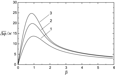
Figure 3: Dependence of $\overline{\Delta\varphi}$ on the impact parameter for $a_{\max}^{2}=0.42$ (1), $a_{\max}^{2}=0.705$ (2), and $a_{\max}^{2}=0.86$ (3); $v=0.8$.

It can be seen that at large $\beta$, the deflection angle behaves in the same way as in the case of the Schwarzschild metric. Fig. 4 shows the deviation of the deflection angle from its averaged value as a function of $\theta_{R}$. As we can see, even with a sufficiently large $a_{\max}^{2}$ the oscillations practically do not differ from sinusoidal ones.

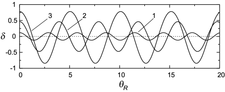
Figure 4: Deviation of the deflection angle from its averaged value, $\delta=(\Delta\varphi-\overline{\Delta\varphi})/\varkappa$, for $a_{\max}^{2}=0.42$ (1), $a_{\max}^{2}=0.705$ (2), and $a_{\max}^{2}=0.86$ (3); $v=0.8,\,\beta=1$.

IV Discussion and concluding remarks

Thus we have considered infinite motion of test particles in time-periodic spherically symmetric spacetimes. Applying the perturbative approach to the geodesic equations, we have obtained general formulas (17)-(19) describing infinite trajectories of the particles passing through oscillating dark matter. From these, formula (20) immediately follows for the total deflection angle of a particle coming from infinity, passing through an oscillating distribution of matter and going to infinity.

As an example, we calculated the deflection angle of a particle passing through an oscillating lump of the self-gravitating scalar field with the logarithmic potential (24). The result is given by Eqs. (38)-(41). It should be noted that the stability of the scalar field lump we were dealing with essentially depends on the amplitude of the oscillations. It turned out that in certain narrow intervals of $a_{\max}$ values, the solutions of the Einstein–Klein–Gordon system with high accuracy retain their periodicity, making hundreds of oscillations, while outside them the solutions, remaining well localized, lose their coherence Koutvitsky2 . This is also true without self-gravity effects Koutvitsky0 ; Koutvitsky5 . We assume that $a_{\max}$ belongs to one of these intervals of quasistability.

The distributions of scalar field dark matter (SFDM) we are considering can be formed by axion-like particles in the ground state determined by the dynamical balance of self-gravity, self-interaction, and quantum pressure. The size of such a structure depends both on the mass of scalar particles and on the self-interaction potential of the scalar field.

It was argued (see Hui and references therein) that in studying DM structures on galactic scales and above, the self-interaction of axion-like particles can be neglected. In this case, the central part of the dark matter configuration, the so-called core, can be described by the system of Schrödinger-Poisson (SP) equations. The characteristic size of this core is roughly equal to the de Broglie wavelength and amounts to $\sim$ 1 kpc for $m\simeq 10^{-22}$ eV, the core mass being limited from above by the value of $10^{12}{M}_{\odot}$ Hui .

On the scales larger than the de Broglie wavelength, the SFDM behaves as cold dark matter, and thus, the solitonic core should be surrounded by a scalar field halo with Navarro-Frenk-White (NFW) density distribution NFW derived from the results of the N-particle modeling. Formation of the soliton-like core in the central region of the SFDM lump was clearly demonstrated in the 3D SP simulation of the ultralight dark matter Schive , where a good fit was provided of the core density profile. These calculations, however, proved to be unable to yield the NFW density profile outside the core.

A comprehensive method for predicting the global density profiles of the SFDM halo was proposed in Robles . It enables to match the fit Schive to the NFW profile. Comparison with circular velocities of the galaxies from the SPARC database with those corresponding to this global density fit shows, however, that this new profile, while provides better agreement with SPARC data at outer radii of galaxies, cannot solve and even exacerbates the central density problem. This fact prompted the authors of Robles to regard baryonic feedback as a probable candidate for resolving this discrepancy.

Another approach to the problem of the galactic core is based on the assumption that the core consists of a central black hole surrounded by a self-gravitating scalar field. For the case of a massive real scalar field without self-interaction, oscillating long-lived self-gravitating configurations of the scalar field around a non-rotating black hole were found in Ref. Sanch by numerically solving the Einstein-Klein-Gordon equations. For a complex non-self-interacting scalar field, such configurations were found in Ref. Barranco3 in the form of self-gravitating coherent states. The authors believe that these configurations can be detected due to their influence on behavior of light rays, stars, gas clouds or other compact objects surrounding a black hole in the center of galaxies. In this context, we note that our results obtained in the weak field approximation lose their validity near the horizon of the black hole, but remain valid for large values of the impact parameter $b\gg r_{g}$, if the oscillation amplitude of the scalar field is not too large.

The inclusion of self-interaction in the consideration can significantly change the expected properties of dark matter distributions. Therefore, the shape and parameters of the scalar field potential should be chosen from the observational data. Thus, in Ref. Amaro strong restrictions on the axion mass and self-interaction coupling constant based on astrophysical and cosmological observations were found for the $\phi^{2}-\phi^{4}$ potential. It turned out that these restrictions do not allow such a potential to be suitable for describing both dark matter halos and compact dark matter objects like boson stars. As was shown in Ref. Arbey , the mass of the scalar field and the self-interaction constant in this potential almost uniquely determine the characteristic scale of the scalar lumps. This means that if these parameters are fixed, then all the halos considered in this model as giant boson stars would have practically the same size, in stark disagreement with observations. Apparently, the only way to overcome this difficulty is to assume that galactic halos are collisionless ensembles of small-scale components of scalar dark matter, rather than whole giant lumps of the scalar dark matter field. These components, the so-called mini-massive compact halo objects Hernandez , static or oscillating, should be of star-size or smaller and have a mass less than $10^{-7}M_{\odot}$ following from microlensing data Alcock . This idea was further developed in Ref. Barranco4 , where the Einstein-Klein-Gordon system with the axion self-interaction potential was solved numerically in the quasi-classical limit. Having chosen the axion mass $m\sim 10^{-5}$ eV and the decay constant $f\sim 6\times 10^{20}$ eV, the authors found the self-gravitating lumps of the axion field with the mass of an asteroid ($\sim 10^{-16}M_{\odot}$) and radius of a few meters.

In our toy model with logarithmic potential (24), it is assumed that the self-interaction dominates gravity, since we work in the weak field approximation. In the limiting case when gravity is neglected, the considered oscillating lump becomes the exact pulson solution of the Klein-Gordon equation with the characteristic size $\sim m^{-1}$. The inclusion of weak gravity practically does not change the size of the lump, so that its compactness remains the same, $\sim\left(e\sqrt{\pi}\right)^{3}\sigma^{2}V_{\max}$, where $\sigma^{2}\ll G^{-1}$ is assumed (see Koutvitsky2 for details). Thus, at $m\sim 10^{-22}$ eV, the lump size is about $0.06$ pc, that is much smaller than the galactic core size, and much larger than the star size. As for the period $T_{g}$, it can be seen from Fig. 2 that in a rather wide range of $a_{\max}^{2}$values, we can take $T\simeq 10$, so that $T_{g}\approx\left(2m\right)^{-1}T\sim 1$ year. To obtain the Sun-sized lump we need to assume $m\simeq 2.7\times 10^{-16}$ eV, that gives $T_{g}\simeq 12$ seconds. Such lumps must have a very low average density $\rho\lesssim 10^{-7}\rho_{\odot}$, which means the weakness of the gravitational field everywhere, including their interior. Nevertheless, we believe that multiple gravitational scattering of particles by an ensemble of these lumps with random oscillation phases can make an additional contribution to the isotropization of cosmic rays and cause small variations of neutrino flux from supernovae.

References

- (1) J. R. Primack, New J. Phys. 11, 105029 (2009).
- (2) D. J. E. Marsh, Phys. Rept. 643, 1 (2016).
- (3) M. S. Turner, Phys. Rev. D 28, 1243. (1983).
- (4) E. Seidel and W.-M. Suen, Phys. Rev. Lett. 66, 1659 (1991).
- (5) E. Seidel and W.-M. Suen, Phys. Rev. Lett. 72, 2516 (1994).
- (6) E. W. Kolb and I. I. Tkachev, Phys. Rev. D 49, 5040. (1994).
- (7) J.-W. Lee and I.-G. Koh, Phys. Rev. D 53, 2236. (1996).
- (8) P. J. E. Peebles, Astrophys. J. 534, L127 (2000).
- (9) W. Hu, R. Barkana, and A. Gruzinov, Phys. Rev. Lett. 85, 1158 (2000).
- (10) T. Matos, F. S. Guzmán, and D. Nunez, Phys. Rev. D 62, 061301(R) (2000).
- (11) J. Magaña, T. Matos, V. H. Robles, and A. Suárez, J. Phys. Conf. Ser. 378, 012012 (2012).
- (12) L. Hui, J. P. Ostriker, S. Tremaine, and E. Witten, Phys. Rev. D 95, 043541 (2017).
- (13) M. Khlopov, B. Malomed, and Ya. Zeldovich, Mon. Not. R. Astron. Soc. 215, 575 (1985).
- (14) L. Kofman, A. Linde, and A. A. Starobinsky, Phys. Rev. Lett. 73, 3195 (1994).
- (15) V. A. Koutvitsky and E. M. Maslov, J. Math. Phys. 47, 022302 (2006).
- (16) M. A. Amin, R. Easther, H. Finkel, R. Flauger, and M. P. Hertzberg, Phys. Rev. Lett. 108, 241302 (2012).
- (17) U.-H. Zhang, and T. Chiueh, Phys. Rev. D 96, 063522 (2017).
- (18) K. D. Lozanov and M. A. Amin, Phys. Rev. D 97, 023533 (2018).
- (19) V. A. Koutvitsky and E. M. Maslov, J. Math. Phys. 59, 113504 (2018).
- (20) H. Fukunaga, N. Kitajima, and Y. Urakawa, J. Cosmol. Astropart. Phys. 06 (2019) 055.
- (21) A. Arvanitaki, S. Dimopoulos, M. Galanis, L. Lehner, J. O. Thompson, and K. Van Tilburg, Phys. Rev. D 101, 083014 (2020).
- (22) J. Olle, O. Pujolas, and F. Rompineve, J. Cosmol. Astropart. Phys. 02 (2020) 006.
- (23) L. A. Ureña-Lopez, Classical Quantum Gravity 19, 2617 (2002).
- (24) G. Fodor, P. Forgács, and M. Mezei, Phys. Rev. D 82, 044043 (2010).
- (25) V. A. Koutvitsky and E. M. Maslov, Phys. Rev. D 83, 124028 (2011).
- (26) F. S. Guzmán and L. A. Ureña-Lopez, Astrophys. J. 645, 814819 (2006).
- (27) A. Khmelnitsky and V. Rubakov, J. Cosmol. Astropart. Phys. 02 (2014) 019.
- (28) A. Aoki and J. Soda, Int. J. Mod. Phys. D 26, 1750063 (2017).
- (29) D. Blas, D. L. Nacir, S. Sibiryakov, Phys. Rev. Lett. 118, 261102 (2017).
- (30) M. Rozner, E. Grishin, Y. B. Ginat, A. P. Igoshev, and V. Desjacques, J. Cosmol. Astropart. Phys. 03 (2020) 061.
- (31) R. Becerril, T. Matos, and L. Ureña-López, Gen. Relativ. Gravit. 38, 633 (2006).
- (32) M. Bošković, F. Duque, M. C. Ferreira, F. S. Miguel, and V. Cardoso, Phys. Rev. D 98, 024037 (2018).
- (33) V. A. Koutvitsky and E. M. Maslov, Theor. Math. Phys. 201, 1793 (2019).
- (34) V. A. Koutvitsky and E. M. Maslov, Phys. Rev. D 102, 064007 (2020).
- (35) G. Rosen, Phys. Rev. 183, 1186 (1969).
- (36) I. Bialynicki-Birula and J. Mycielski, Bull. Acad. Pol. Sci., Sér. sci. tech. 23, 461 (1975).
- (37) A. Linde, Phys. Lett. B 284, 215 (1992).
- (38) J. D. Barrow and P. Parsons, Phys. Rev. D, 52, 5576 (1995).
- (39) K. Enqvist and J. McDonald, Phys. Lett. B, 425, 309 (1998).
- (40) G. C. Marques and I. Ventura, Rev. Bras. Fis. 7, 297 (1977).
- (41) I. L. Bogolubsky, JETP 49, 213 (1979).
- (42) E. M. Maslov, Phys. Lett. A 151, 47 (1990).
- (43) S. Weinberg, Gravitation and Cosmology (John Wiley & Sons, New York, 1972).
- (44) V. A. Koutvitsky and E. M. Maslov, Phys. Lett. A 336, 31 (2005).
- (45) J. F. Navarro, C. S. Frenk, and S. D. M. White, Astrophys. J., 490, 493 (1997).
- (46) H.-Y. Schive, T. Chiueh, and T. Broadhurst, Nature Physics, 10, 496 (2014).
- (47) V. H. Robles, J. S. Bullock, and M. Boylan-Kolchin, Mon. Not. R. Astron. Soc., 483, 289 (2019).
- (48) N. Sanchis-Gual, J. C. Degollado, P. J. Montero, and J. A. Font, Phys. Rev. D 91, 043005 (2015).
- (49) J. Barranco, A. Bernal, J. C. Degollado, A. Diez-Tejedor, M. Megevand, D. Núñez, and O. Sarbach, Phys. Rev. D 96, 024049 (2017).
- (50) P. Amaro-Seoane, J. Barranco, A. Bernal, and L. Rezzolla, J. Cosmol. Astropart. Phys. 11 (2010) 009.
- (51) A. Arbey, J. Lesgourgues, and P. Salati, Phys. Rev. D 68, 023511 (2003).
- (52) X. Hernández, T. Matos, R. A. Sussman, and Y. Verbin, Phys. Rev. D, 70, 043537 (2004).
- (53) C. Alcock at al., Astrophys. J. Lett. 499, L9 (1998).
- (54) J. Barranco and A. Bernal, Phys. Rev. D 83, 043525 (2011).