Positive-Unlabeled Learning with Uncertainty-aware Pseudo-label Selection

Abstract

Positive-unlabeled (PU) learning aims at learning a binary classifier from only positive and unlabeled training data. Recent approaches addressed this problem via cost-sensitive learning by developing unbiased loss functions, and their performance was later improved by iterative pseudo-labeling solutions. However, such two-step procedures are vulnerable to incorrectly estimated pseudo-labels, as errors are propagated in later iterations when a new model is trained on erroneous predictions. To prevent such confirmation bias, we propose PUUPL, a novel loss-agnostic training procedure for PU learning that incorporates epistemic uncertainty in pseudo-label selection. By using an ensemble of neural networks and assigning pseudo-labels based on low-uncertainty predictions, we show that PUUPL improves the reliability of pseudo-labels, increasing the predictive performance of our method and leading to new state-of-the-art results in self-training for PU learning. With extensive experiments, we show the effectiveness of our method over different datasets, modalities, and learning tasks, as well as improved calibration, robustness over prior misspecifications, biased positive data, and imbalanced datasets.

1 Introduction

Many real-world applications involve positive-unlabeled (PU) datasets [1, 2, 3] in which only small parts of the data is labeled positive while the majority is unlabeled. Learning from PU data can reduce development costs in many deep learning applications that otherwise require annotations from experts such as medical image diagnosis [1], protein function prediction [2], and it can even enable applications in settings where the measurement technology itself can not detect negative examples [3].

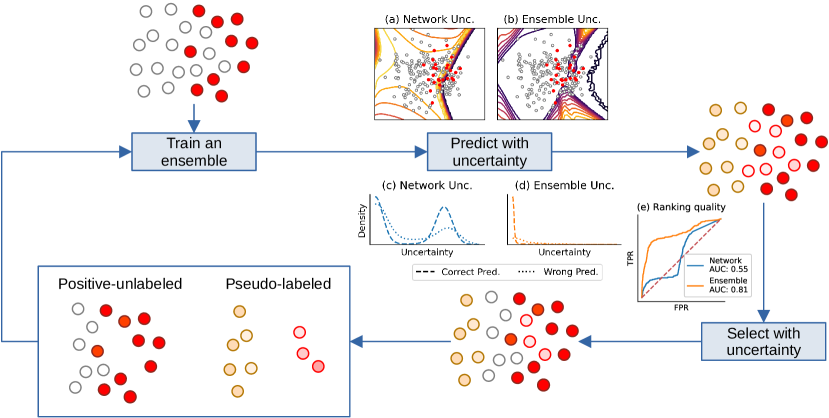
Figure 1: PUUPL is a pseudo-labeling framework for PU learning that uses the epistemic uncertainty of an ensemble to select confident examples to pseudo-label. The ensemble can be trained with any PU loss for PU data while minimizing the cross-entropy loss on the previously assigned pseudo-labels. In a toy example, a single network is not very confident on most of the unlabeled data (a), resulting in many high-confidence incorrect predictions and many low-confidence correct ones (c). The epistemic uncertainty of an ensemble is, on the other hand, very low on most of the unlabeled data (b), resulting in most correct predictions having low uncertainty and most incorrect predictions having high uncertainty (d). Thus, the estimated uncertainty by ensemble can be used more reliably to rank predictions and select correct ones (e). Re-training the model with an increased number of labeled samples will result in a slightly more accurate model, than can be used to predict new pseudo-labels, which will further improve the model’s performance, etc.

Approaches such as unbiased PU [4] and non-negative PU [5] formulate this problem as cost-sensitive learning and sparked a stream of works on risk estimators for PU learning (PUL). Others approach PUL as a two-step procedure, first identifying and labeling some reliable negative examples, and then re-training the model based on this newly constructed labeled dataset [6]. These approaches show similarities with pseudo-labeling in semi-supervised classification settings [7] and are generally able to reach higher performance compared to other methods that use a single training iteration. Such pseudo-labeling techniques are however especially vulnerable to incorrectly assigned labels of the selected examples as such errors will propagate and magnify in the retrained model, resulting in a negative feedback loop. This erroneous selection of unreliable pseudo-labels occurs when wrong model predictions are associated with excessive model confidence, which is accompanied by a distortion of the signal for the pseudo-label selection [8]. In recent literature on pseudo-labeling, this problem, also referred to as confirmation bias [9], is recognized and successfully addressed by explicitly estimating the prediction uncertainty [10, 11]. While this is the case for semi-supervised classification, recent self-training approaches for PUL do not explore the use of uncertainty quantification for pseudo-labeling in this context.

Contributions: Motivated by this, we propose a novel framework for PUL that leverages uncertainty quantification to identify reliable examples to pseudo-label (Fig. 1). In particular,

1. We introduce PUUPL (Positive Unlabeled, Uncertainty aware Pseudo-Labeling), a novel framework that successfully overcomes the issue of confirmation bias in PUL.

2. We evaluate our methods on a wide range of benchmarks and PU datasets, achieving state-of-the-art results in self-training for PUL both with and without known positive class prior $\pi=p(y=1)$.

3. Through extensive experiments we show that PUUPL results in very well-calibrated predictions, is applicable to different data modalities such as images and text, can use any risk estimator for PUL and improve thereupon, and is robust to prior misspecification and class imbalance.

These results show our framework to be highly reliable, extensible, and applicable in a wide range of real world scenarios.

2 Related work

Positive-unlabeled learning PUL was introduced as a variant of binary classification [12] and is related to one-class learning [13, 14], multi-positive learning [15], multi-task learning [16], and semi-supervised learning [17]. Current existing methods for PUL can be divides into three branches: two-step techniques, class prior incorporation, and biased PUL [6]. In this work, we apply pseudo-labeling with biased PUL – also coined as reweighting methods – and refer to [6] for a comprehensive overview of the field. In this context, [4] introduced the unbiased risk estimator uPU. [5] showed that this loss function is prone to overfitting in deep learning contexts, as it lacks a lower bound, and proposed the non-negative risk estimator nnPU as a remedy. Follow-up work on loss functions for PUL has focused on robustness w.r.t. biases in the sampling process [18, 19, 20] and handling of imbalanced datasets [21]. Further works in PUL focused on estimating the class prior directly during training [22, 23, 24] or exploiting its knowledge to further improve the training process [25, 26, 27, 28].

Uncertainty-aware pseudo-labeling Pseudo-labeling follows the rationale that the model leverages its own predictions on unlabeled data as pseudo-training targets to enable iterative semi-supervised model training. The first such approach for deep learning was introduced by [7] in which the class with the highest predicted probability was simply selected as a pseudo label. One weakness of pseudo-labeling is that erroneously selected pseudo-labels can amplify during training, potentially leading to model degradation. This confirmation bias grounded in poor model calibration is distorting the signal for the pseudo label selection [8]. [29] tried to mitigate this issue using confidence and class weights. [30] used confidence scores based on the geometric neighborhood of the unlabeled samples, while [9] effectively tackled the confirmation bias using mixup [31], Label Noise [32], and Entropy Regularization [33]. [11] introduced a pseudo-labeling framework using a weighting scheme for class balancing and Monte Carlo dropout [34] for calibration, while [35] found that deep ensembles [36] yield the best model calibration in an active learning context, especially in low-label regimes. The commonality of these works is the explicit consideration of model uncertainty to improve pseudo-label selection, which motivates its application in the context of PUL.

Pseudo-labeling for PUL Two-step approaches in PUL first identify negative samples from the unlabeled dataset and then train a binary classification model on the original dataset augmented with the newly identified negatives [6]. These approaches share similarities with pseudo-labeling but lack an iterative feedback loop after the completion of the second step. A first attempt to combine pseudo-labeling with PUL was made with Self-PU [25], where self-paced learning, a confidence-weighting scheme based on the model predictions, and a teacher-student distillation approach are combined. With PUUPL, we propose an alternative pseudo-labeling strategy for PUL that performs better in a simpler and more principled way using implicitly well-calibrated models to improve the pseudo-label selection.

Uncertainty-aware pseudo-labeling for PUL To the best of our knowledge, we are the first to introduce an uncertainty-aware pseudo-labeling paradigm to PUL. Although our method shares the same motivation as that from [11] for semi-supervised classification, we differ in several important aspects: (1) we specifically target PU data with a PU loss, (2) we quantify uncertainty with an ensemble instead of Monte Carlo dropout, (3) we use epistemic uncertainty instead of the predicted class probabilities for the selection, (4) we do not use temperature scaling, (5) we use soft labels and (6) we explicitly identify advantages of PL in a PU setting.

3 Method

PUUPL (Algorithm 1) separates the training set $X^{tr}$ into the sets $P$, $U$, and $L$, which contain the initial positives, the currently unlabeled, and the pseudo-labeled samples, respectively. The set $L$ is initially empty. At each pseudo-labeling iteration, we first train our model using all samples in $P$, $U$, and $L$ until some convergence condition is met (Section 3.2). Then, samples in $U$ are predicted and ranked w.r.t. their predictive uncertainty (Section 3.3), and samples with the most confident score are assigned the predicted label and moved into the set $L$ (Section 3.4). Similarly, samples in $L$ are also predicted, and the most uncertain samples are moved back to the unlabeled set $U$ (Section 3.5). Next, the model is re-initialized to the same initial weights, and the next pseudo-labeling iteration starts.

3.1 Notation

Consider input samples $X$ with label $y$ and superscripts ${\cdot}^{tr}$, ${\cdot}^{va}$ and ${\cdot}^{te}$ for training, validation, and test data, respectively. The initial training labels $y^{tr}$ are set to one for all samples in $P$ and zero for all others in $U$. We group the indices of original positives, unlabeled, and pseudo-labeled samples in $X^{tr}$ into the sets $P$, $U$, and $L$, respectively. Our proposed model is an ensemble of $K$ deep neural networks whose random initial weights are collectively denoted as $\theta^{0}$. The predictions of the $k$-th network for sample $i$ are indicated with $\hat{p}_{ik}=\sigma(\hat{f}_{ik})$, with $\sigma(\cdot)$ as the logistic function and $\hat{f}_{ik}$ as the predicted logits. The logits and predictions for a sample averaged across the networks in the ensemble are denoted by $\hat{f}_{i}$ and $\hat{p}_{i}$, respectively. We subscript data and predictions with $i$ to index individual samples, and use an index set in the subscript to index all samples in the set (e.g., $X^{tr}_{U}=\{X^{tr}_{i}|i\in U\}$ denotes the features of all unlabeled samples). We denote the total, epistemic, and aleatoric uncertainty of sample $i$ as $\hat{u}^{t}_{i}$, $\hat{u}^{e}_{i}$, and $\hat{u}^{a}_{i}$, respectively.

Algorithm 1 The PUUPL Training Procedure

Hyperparameters:

• Loss mixing coefficient $\lambda$ (suggested $\lambda=0.1$)

• Number $K$ of networks in the ensemble (suggested $K=2$)

• Maximum number $T$ of pseudo-labels to assign at each round (suggested $T=1000$)

• Maximum uncertainty threshold $t_{l}$ to assign pseudo-labels (suggested $t_{l}=0.05$)

• Minimum uncertainty threshold $t_{u}$ to remove pseudo-labels (suggested $t_{u}=0.35$)

Input: Train and validation $X^{tr},y^{tr},X^{va},y^{va}$

1:$P\leftarrow$ indices of positive samples in $X^{tr}$

2:$U\leftarrow$ indices of unlabeled samples in $X^{tr}$

3:$L\leftarrow\emptyset$

4:$\theta^{0}\leftarrow$ Random weight initialization

5:while not converged do

6:    Initialize model weights to $\theta^{0}$

7:    Train an ensemble of $K$ networks on $X^{tr},y^{tr}$

8:    Update $\theta^{*}$ if performance on $X^{va},y^{va}$ improved

9:    $\hat{f}\leftarrow$ ensemble predictions for $X^{tr}$

10:    Compute epistemic uncertainty via Eq. 6

11:    $L^{\text{new}}\leftarrow$ Examples to pseudo-label via Eq. 7

12:    $U^{\text{new}}\leftarrow$ Examples to pseudo-unlabel

13:    $L\leftarrow L\cup L^{\text{new}}_{b}\setminus U^{\text{new}}$

14:    $U\leftarrow U\setminus L^{\text{new}}_{b}\cup U^{\text{new}}$

15:    $y_{L^{\text{new}}}\leftarrow\hat{p}_{L^{\text{new}}}$

16:    $y_{U^{\text{new}}}\leftarrow 0$

17:end while

3.2 Loss function

We train our proposed model with a loss function $\mathcal{L}$ that is a convex combination of a loss $\mathcal{L}_{PU}$ for the samples in the positive and unlabeled set ($P\cup U$) and a loss $\mathcal{L}_{L}$ for the samples in the pseudo-labeled set ($L$):

$$\mathcal{L}=\lambda\cdot\mathcal{L}_{L}+(1-\lambda)\cdot\mathcal{L}_{PU}$$ (1)

with $\lambda\in(0,1)$. The loss $\mathcal{L}_{L}$ is the binary cross-entropy computed w.r.t. the assigned pseudo-labels $y$. Our method is agnostic to the specific PU loss $\mathcal{L}_{PU}$ used, allowing PUUPL to be easily adapted to provide further performance increase in other scenarios for which a different PU loss might be more appropriate, e.g., when a set of biased negative samples is available [19], when coping with a selection bias in the positive examples [18] or an imbalanced class distribution [21] (see experiments). For the standard setting of PUL, we use the non-negative correction $nnPU$ of the PU loss [5]:

$$\mathcal{L}_{PU}=\pi\cdot\ell(P,1)+\max\left\{0,\ell(U,-1)-\pi\cdot\ell(P,-1)\right\}$$ (2)

where $\pi=p(y=1)$ is the prior probability that a sample is positive and $\ell(S,y)$ the expected sigmoid loss of samples in the set $S$ with label $y$:

$$\ell(S,y)=\frac{1}{|S|}\sum_{i\in S}\frac{1}{1+\exp(y\cdot\hat{p}_{i})}$$ (3)

While $\pi$ can be estimated from PU data [37], in our experimental results we treat $\pi$ as a hyperparameter and optimize it without requiring negatively labeled samples [38].

3.3 Model uncertainty

To quantify the predictive uncertainty, we utilize a deep ensemble with $K$ networks with the same architecture, each trained on the full training dataset [36]. Given the predictions $\hat{p}_{i1},\ldots,\hat{p}_{iK}$ for a sample $x_{i}$, we associate three types of uncertainties to $x_{i}$’s predictions [39]: the aleatoric uncertainty as the mean of the entropy of the predictions (Eq. 4), the total uncertainty as the entropy of the mean prediction (Eq. 5), and the epistemic uncertainty formulated as the difference between the two (Eq. 6).

$$\hat{u}^{a}_{i} =-\frac{1}{K}\sum_{k=1}^{K}\left[\hat{p}_{ik}\log\hat{p}_{ik}+(1-\hat{p}_{ik})\log(1-\hat{p}_{ik})\right]$$ (4)

$$\hat{u}^{t}_{i} =-\hat{p}_{i}\log\hat{p}_{i}-(1-\hat{p}_{i})\log(1-\hat{p}_{i})$$ (5)

$$\hat{u}^{e}_{i} =\hat{u}^{t}_{i}-\hat{u}^{a}_{i}$$ (6)

where $\hat{p}_{i}=\sum_{k=1}^{K}\hat{p}_{ik}/K$. Epistemic uncertainty corresponds to the mutual information between the parameters of the model and the true label of the sample. Low epistemic uncertainty thus means that the model parameters would not change significantly if trained on the true label, suggesting that the prediction is indeed correct. The cumulative effect of many correct pseudo-labels added over time, however, is enough to push the model towards better-performing parameters, as we show in the experimental results.

3.4 Pseudo-labeling

The estimated epistemic uncertainty (Eq. 6) is used to rank and select unlabeled examples for pseudo-labeling. Let $\rho(i)$ denote the rank of sample $i$. Then, the set $L^{\text{new}}$ of newly pseudo-labeled samples is formed by taking the $T$ samples with lowest uncertainty from $U$, ensuring that it is lower than a threshold $t_{l}$:

$$L^{\text{new}}=\left\{i\in U|\rho(i)\leq T\land u^{e}_{i}\leq t_{l}\right\}\\$$ (7)

Previous works have shown that balancing the pseudo-label selection between the two classes – i.e., ensuring that the ratio of newly labeled positives and negatives is close to a given target ratio $r$ – is beneficial [11]. In this case, the set $L^{\text{new}}$ is partitioned according to the model’s predictions into a set $L^{\text{new}}_{+}$ of predicted positives and $L^{\text{new}}_{-}$ of predicted negatives, and the most uncertain samples in the larger set are discarded to reach the desired ratio $r$, which we fix to $1$. We then assign soft pseudo-labels, i.e., the average prediction in the open interval $(0,1)$, to these samples:

$$y_{i}=\hat{p}_{i}\quad\forall i\in L^{\text{new}}_{-}\cup L^{\text{new}}_{+}$$ (8)

As discussed previously, low epistemic uncertainty signals likely correct predictions. Using such predictions as a target in the loss $\mathcal{L}_{L}$ provides a stronger, more explicit learning signal to the model, resulting a larger decrease in risk compared to using the same example as unlabeled in $\mathcal{L}_{PU}$ At the same time, soft pseudo-labels provide an additional signal regarding the estimated aleatoric uncertainty of samples and, by acting as dynamically-smoothed labels, they help reduce overfitting and the emergence of confirmation bias [40, 9] in case the assigned pseudo-label is wrong.

3.5 Pseudo-unlabeling

Similar to the way that low uncertainty on an unlabeled example indicates that the prediction can be trusted, high uncertainty on a pseudo-labeled example indicates that the assigned pseudo-label might not be correct after all. To avoid training on such possibly incorrect pseudo-labels, we move the pseudo-labeled examples with uncertainty above a threshold $t_{u}$ back into the unlabeled set:

$$U^{\text{new}}=\left\{i\in L|\hat{u}^{e}_{i}\geq t_{u}\right\}$$ (9)

$$y_{i}=0\quad\forall i\in U^{\text{new}}$$ (10)

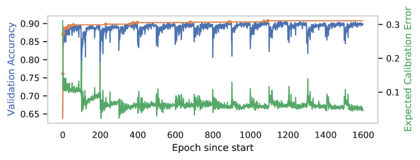
Figure 2: Validation accuracy (left, blue) and expected calibration error (ECE, right, green) for a run on CIFAR-10 with 1,000 positives. Note the substantial reduction in ECE in the second and third pseudo-labeling iterations, when the ensemble is trained on soft labels. The orange line indicates the best validation accuracy at each epoch, with the new highest accuracy marked by orange dots. The overall highest was 90.76% at epoch 1092, corresponding to a test accuracy of 90.35%.

	Dataset
Method	MNIST	F-MNIST	CIFAR-100-20	CIFAR-10	IMDb	Notes
Self-PU [25]†	95.64 $\pm 0.13$	91.55 $\pm 0.18$	75.41 $\pm 0.44$	90.56 $\pm 0.09$	00– $\pm 0.00$	Baselines
VPU [22]	93.84 $\pm 0.88$	91.90 $\pm 0.22$	72.12 $\pm 1.05$	87.50 $\pm 1.05$	00– $\pm 0.00$
nnPU [5]	96.20 $\pm 0.03$	92.73 $\pm 0.06$	72.78 $\pm 0.41$	90.84 $\pm 0.09$	78.56 $\pm 0.75$	Highest test accuracy
+PL	96.56 $\pm 0.05$∗∗∗	92.79 $\pm 0.05$	75.85 $\pm 0.44$∗∗∗	91.27 $\pm 0.07$∗∗∗	80.91 $\pm 0.47$∗∗∗
+PUUPL	96.89 $\pm 0.04$∗∗∗	92.89 $\pm 0.04$∗	76.50 $\pm 0.34$.	91.37 $\pm 0.05$.	82.02 $\pm 0.13$∗∗∗
nnPU [5]	95.65 $\pm 0.12$	92.14 $\pm 0.08$	74.66 $\pm 0.62$	90.11 $\pm 0.13$	76.90 $\pm 0.81$	PU Validation, Unknown $\pi$
+PL	95.54 $\pm 0.18$	91.95 $\pm 0.23$	74.40 $\pm 0.93$	89.27 $\pm 0.32$∗	79.17 $\pm 1.09$∗
+PUUPL	95.99 $\pm 0.19$∗	92.43 $\pm 0.11$∗∗∗	76.18 $\pm 0.15$ ∗	90.27 $\pm 0.23$∗∗∗	80.81 $\pm 0.35$∗∗∗

Table 1: Test accuracy, standard error, and statistical significance over ten runs on various datasets with 3,000 labeled positives except for IMDb where we used 1,000. Bold font indicates highest performance in the two settings of PN and PU validation. The row “+PL“ refers to an naive pseudo-labeling baseline, while “+PUUPL“ refers to our uncertainty-aware solution. Statistical significance established via unpaired, two-tailed $t$-test; PUUPL was compared with the PL baseline, which was in turn compared to nnPU (signif. codes: ***: $p<0.001$, **: $p<0.01$, *: $p<0.05$, .: $p<0.1$). ^† method used a PN labeled validation set and should thus be compared with PUUPL’s highest test accuracy.

4 Experiments

To empirically compare our proposed framework to existing state-of-the-art losses and models, we followed standard protocols for PUL [5, 18, 22, 25] as described in Section 4.1. In Section 4.2, after presenting the main results, we empirically show the advantage of our framework in providing well-calibrated predictions, improving performance with imbalanced datasets, being applicable to different data modalities, and using various losses for PU learning. Finally, in Section 4.3 we discuss the sensitivity of PUUPL with respect to pseudo-labeling hyperparameters.

4.1 Experimental protocol

Datasets: We evaluated our method in the standard setting of MNIST [41] and CIFAR-10 [42] datasets, as well as Fashion MNIST (F-MNIST) [43], CIFAR-100-20 [42] and IMDb [44] to show the applicability to different data modalities. Similar to previous studies [22, 5, 18, 25], positives were defined as odd digits in MNIST and vehicles in CIFAR-10. For F-MNIST we used trousers, coats, and sneakers as positives, and for the experiments on CIFAR-100-20 we defined those 10 out of 20 superclasses as Positives that correspond to living creatures (i.e., ‘aquatic mammal‘, ‘fish‘, ‘insects‘, ‘large carnivores‘, ‘large omnivores‘, ‘medium-sized mammals‘, ‘non-insect invertebrates‘, ‘people‘, ‘reptiles‘, ‘small mammals‘). The number of training samples is reported in Supplementary Table 5.

For all datasets, we reserved a validation set of 5,000 samples and used all other samples for training, evaluating on the canonical test set. We used either 1,000 or 3,000 (except for IMDb) randomly chosen labeled positives in the training set, as is common practice, and used the same proportion of labeled to unlabeled in the validation set (e.g., the validation set for CIFAR-10 contained 111 labeled positives and 4,889 unlabeled samples). For the image datasets, we subtracted the mean pixel intensity in the training set and divided it by the standard deviation, while for IMDb we used pre-trained GloVe embeddings of size 200 on a corpus of six billion tokens.

Network architectures: To ensure a fair comparison with other works in PUL [25, 22, 5], we used the same architectures on the same datasets, namely a 13-layer convolutional neural network (CNN) for the experiments on CIFAR-10 and CIFAR-100-20 (Table 6) and a multi-layer perceptron (MLP) with four fully-connected hidden layers of 300 neurons each and ReLU activation for MNIST and F-MNIST. For IMDb, we used a bidirectional LSTM network with a MLP head whose number of units were optimized as part of the hyperparameter search (Table 7).

Training: We trained all models with the Adam optimizer [45] with $\beta_{1}=0.9$ and $\beta_{2}=0.999$ and an exponential learning rate decay with $\gamma=0.99$, while learning rate, batch size and weight decay were tuned via Hyperband [46] (see below). We further used the nnPU loss [5] as $\mathcal{L}_{PU}$ unless otherwise stated. We provide experimental results using both a PU validation set, to provide a real-world performance estimate, as well as a fully-labeled (PN) validation set to compare against PUL methods that used such a labeled validation set [25, 24] and to showcase the potential of our method. When using a PU validation set, we used the AUC between positive and unlabeled samples as criterion, as previous work [38, 47] has shown that higher PU-AUC directly translates to higher AUC on fully labeled data.

Hyperparameter tuning: We used the same pseudo-labeling hyperparameters, constituting the suggested defaults in Algorithm 1, across all datasets and data modalities. These hyperparameters were optimized on CIFAR-10 using the Hyperband algorithm [46] with $\eta=3$ and $s=4$, with the ranges used in the process reported in Table 8. On the other datasets, we only tuned the prior $\pi$ and hyperparameters related to network training such as batch size, learning rate, weight decay, number of training epochs, dropout probability, and other details of the network architecture by running only the first bracket of Hyperband with $\eta=3$ and $S=3$.

Evaluation: The best configuration found by Hyperband was trained ten times with different random initializations and training/validation splits and evaluated on the test set to produce the final results. We reported both the highest test accuracy obtained and the test accuracy when a PU validation set was used, resulting in a total of 18 experiments. We compared PUUPL against VPU [22] and Self-PU [25] using the same network architecture and data splits. We consider the former as it does not require a known prior $\pi$, and the latter as the state-of-the-art self-training method for PUL. We additionally compare against a naive, uncertainty-unaware, pseudo-labeling baseline “+PL“ that used the raw sigmoid outputs as a ranking measure for pseudo-labeling, while still assigning soft pseudo-labels.

4.2 Results

PUUPL achieved the highest test accuracy in 15 out of 18 experiments, and the difference was statistically significant in 12 cases (Table 1 in the main text and Table 9 in the Supplement). Only on F-MNIST with 1,000 positives and PU validation PUUPL was statistically-significantly worse than the top performer, the naive pseudo-labeling baseline ($0.6\%$ lower test accuracy), however no statistically-significant difference was found against nnPU and VPU (Self-PU needs a labeled validation set, thus it is not applicable in this setting). On the other hand, in several datasets PUUPL increased the test performance by up to four percentage points, corresponding to reductions in error rates of up to 16% and more on imbalanced data (as we show in detail below). These findings substantiate the advantages of pseudo-labeling in PUL as well as the necessity of uncertainty quantification in this procedure. In the remaining part of this section, we present the results of selected experiments aimed at showing the benefits of PUUPL in practical applications, and provide further robustness studies in Supplementary Section A.3.

	nnPU	+PL	+PUUPL
Test Expected Calibration Error (%)
MNIST	4.26$\pm 0.10$	3.61$\pm 0.09$	1.96$\pm 0.09$
CIFAR-10	10.89$\pm 0.10$	9.24$\pm 0.15$	5.70$\pm 0.72$
CIFAR-100-20	31.62$\pm 0.29$	27.51$\pm 0.59$	22.12$\pm 0.39$
Test Negative Log-Likelihood
MNIST	0.21$\pm 0.01$	0.18$\pm 0.01$	0.13$\pm 0.01$
CIFAR-10	1.25$\pm 0.11$	0.76$\pm 0.05$	0.32$\pm 0.02$
CIFAR-100-20	5.26$\pm 0.52$	3.62$\pm 0.22$	1.25$\pm 0.58$
Pseudo-labels Negative Log-Likelihood
MNIST	0.00– $\pm 0.00$	0.05$\pm 0.01$	0.09$\pm 0.01$
CIFAR-10	0.00– $\pm 0.00$	0.66$\pm 0.05$	0.29$\pm 0.03$
CIFAR-100-20	0.00– $\pm 0.00$	3.76$\pm 0.29$	0.94$\pm 0.05$

Table 2: Comparison of expected calibration error(ECE) and negative log-likelihood (NLL) on the test set of three datasets when 1,000 labeled positives were used for training (average and standard error over ten runs). We show the NLL with respect to the test predictions as well as the pseudo-labels against the true labels. PUUPL considerably improved calibration and likelihood compared to nnPU and naive pseudo-labeling (all differences with PUUPL were highly statistically significant, $p<0.0001$).

PUUPL is well calibrated: Good calibration means that the model’s outputs can be interpreted as probabilities instead of being a mere ranking measure. It is a desirable property for practitioners in general and essential in safety-critical applications including in clinical and medical domains [48] and autonomous driving  [49], as well as when fairness is of concern [50]. Moreover, model calibration in a PU setting is particularly challenging as no labeled negatives are available, making popular post hoc and likelihood-based methods such as the Laplace approximation [51], temperature scaling [52], and Bayesian approaches [53] not applicable.

We found that PUUPL was substantially better calibrated than both nnPU and the naive pseudo-labeling baseline (Table 2). In particular, the improvement in expected calibration error (ECE) and negative log-likelihood (NLL) by PUUPL was at least 40% and often much larger. We hypothesize that such improvement stemmed from explicitly incorporating uncertainty in PUUPL, which resulted in improved pseudo-labels. Indeed, PUUPL assigned more accurate pseudo-labels compared to the naive baseline as measured by the cross-entropy between pseudo- and true labels (Table 2). In turn, such improved pseudo-labels led to higher predictive performance as measured in terms of accuracy, NLL and ECE. In fact, as shown in Figure 2 the ECE decreased in the first few pseudo-labeling rounds, and the validation accuracy continued improving after the ECE stabilized.

PUUPL works well with imbalanced datasets: A very common issue faced by practitioners is the presence of imbalanced and heavy-tailed datasets. In traditional supervised learning, it is possible to handle this situation easily by properly adjusting sample weights when computing the loss, and while the same idea applies to PUL, the presence of unlabeled samples makes the problem non-trivial. Nonetheless, an oversampled version of the nnPU loss was developed [21] to handle this scenario and enable PUL with very low priors.

To test our framework in an imbalanced setting, we downsampled the positives in CIFAR-10 to obtain a prior $\pi$ of 0.1 and used only 600 positive labeled samples for training. Pseudo-labeling proved to be particularly effective in this setting, and PUUPL further improved accuracy and calibration, cumulatively reducing the test error rate by 48% compared to nnPU (Table 3). The nnPU loss instead collapsed to constant negative predictions, for a test accuracy of 60%, and both pseudo-labeling strategies were unable to improve performance.

		imbnnPU	+PL	+PUUPL
MNIST
	Accuracy	95.25$\pm 0.15$	95.44$\pm 0.13$	95.66$\pm 0.06$
	ECE (%)	3.53$\pm 0.78$	02.76$\pm 0.62$	02.26$\pm 0.12$
CIFAR-10
	Accuracy	79.99$\pm 1.10$	88.64$\pm 0.26$	89.59$\pm 0.07$
	ECE (%)	19.86$\pm 1.13$	09.36$\pm 0.28$	07.13$\pm 0.56$
CIFAR-100-20
	Accuracy	63.42$\pm 0.66$	68.48$\pm 0.38$	70.88$\pm 0.40$
	ECE (%)	36.65$\pm 1.10$	26.36$\pm 2.28$	24.12$\pm 0.75$

Table 3: Accuracy and expected calibration error (ECE) on the canonical CIFAR-10 test set, where model training was performed with an imbalanced dataset with $\pi=0.1$ and 600 labeled positives. While most of the improvement over the imbnnPU [21] baseline was provided by pseudo-labeling, PUUPL further improved significantly both test accuracy and ECE ($p=0.0026$ and $p=0.0017$ respectively).

	nnPU∗∗∗	nnPUSB∗∗∗
Only PU loss	87.05 $\pm 0.14$∗∗∗	87.31 $\pm 0.12$∗∗
PU loss+PUUPL	87.70 $\pm 0.14$ ∗∗∗	87.91 $\pm 0.14$ ∗∗

Table 4: Test accuracy of PUUPL on the CIFAR-10 dataset with a selection bias on the positive labels when using the nnPU and nnPUSB losses. Our framework significantly improves over the base PU loss in both cases ($p=0.0021$ and $p=0.0022$); in particular, PUUPL with nnPU loss achieved better performance than the nnPUSB loss alone.

PUUPL is loss-agnostic: Our framework is uniquely positioned to take advantage of newly developed risk estimators for PU learning: as we showed above, PUUPL could make use of the imbnnPU loss [21] to greatly improve in the imbalanced setting, but other PU losses exist, too. The nnPUSB loss [18] was developed to address the issue of labeling bias in the training positives, a more general setting compared to the i.i.d. assumption of traditional PUL methods [6]. We tested PUUPL in such a biased setting where positives in the CIFAR-10 training and validation sets were with 50% chance an airplane, 30% chance an automobile, 15% chance a ship, and 5% chance a truck. The test distribution was instead balanced, meaning that test samples were half as likely to be airplanes compared to the training set, and five times more likely to be truck images. We used the same hyperparameters as the i.i.d. CIFAR-10 except for the loss $\mathcal{L}_{PU}$ where we used the nnPUSB loss [18] to handle the positive bias. The baseline with nnPUSB loss performed better than the nnPU loss but worse than PUUPL with the nnPU loss, and the best performance was achieved with PUUPL on top of the nnPUSB loss (Table 4).

These results demonstrate that PUUPL can be applicable even when sampling bias is suspected by a practitioner and no ad hoc risk estimator is available, as our uncertainty-aware pseudo-labeling framework with the bias-oblivious nnPU loss obtained better results compared to a bias-aware risk estimator without pseudo-labeling.

PUUPL is data modality-agnostic: Unlike many alternative methods for PUL, our framework can be applied to learning problems in any domain out of the box as it does not rely on regularization methods that are restricted to a specific data modality, most frequently images, such as mixup [31] (used by [22, 27]) or contrastive representations (used by [26]), is easy to adapt as it builds on standard methods (unlike [25]), and does not require pretrained representations to work (as [28] does).

On the IMDb dataset of movie reviews, PUUPL improved test performance of a LSTM network by four percentage points both with a PU and PN validation set, reducing the test error rate by 16% compared to the nnPU baseline without requiring any modality-specific adaptations.

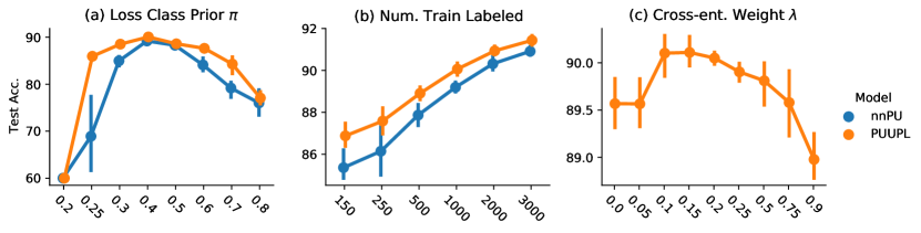
Figure 3: Mean and standard deviation of the CIFAR-10 test accuracy obtained over five runs when training with wrong prior (a), number of training labeled positives (b) and different loss combination parameter $\lambda$ (c). PUUPL proved to be more robust to prior misspecification (true $\pi=0.4$), as the performance degradation was considerably reduced over a wide range of values, and to lower number of labeled samples, as the gap between our framework and nnPU widened as less labeled positives were available for training (note the different $y$-axes scales).

4.3 Sensitivity analysis

In this section, we investigate the sensitivity of PUUPL with respect to class prior $\pi$, loss weighting parameter $\lambda$, and number of training positives by altering each of these parameters and comparing the resulting test performance on CIFAR-10. Further results regarding pseudo-labeling hyperparameters can be found in Supplementary Section A.3.

Prior misspecification: An important concern for practitioners is how to determine the prior $\pi$ of a PU dataset, as in case of sub-optimal estimation the performance of the PU classifier can be harmed considerably. Prior estimation constitutes a whole research branch in PUL [22, 23] and is a significant challenge in any practical PU application [6]. Some contemporary methods for PUL [25, 26, 27, 28] assume a known prior and do not discuss the practical consequences of not knowing such parameter, while other methods incorporate prior estimation directly into the training procedure [22, 23, 24]. We treated $\pi$ as a hyperparameter optimized using the PU-AUC as a criterion [38, 47], thus bridging the gap between estimating the prior during training and assuming it is known a priori.

Our experimental results show that optimizing the prior in such a way resulted in a consistent reduction in test accuracy between 0.8 and 1.2 percentage points for both our framework, nnPU, and the naive pseudo-labeling baseline (Table 1). In a similar vein, methods such as VPU that optimize the prior as part of the training procedure show a similar or larger difference compared to methods that use a labeled validation set such as Self-PU (Supplementary Table 9). However, PUUPL remained the top performer in both settings.

Moreover, training using a wrong value for $\pi$ was less harmful for PUUPL compared to nnPU (Figure 3a). For example, on CIFAR-10 the test accuracy showed a wide plateau around the true prior of 0.4 with a performance reduction of less than 2.5% in the range $[0.3,0.6]$. With smaller priors the nnPU loss collapsed to constantly predicting the majority class, and specialized oversampled risk estimators [21] were needed for such a setting (we showed the effectiveness of PUUPL in imbalanced settings in the previous section). Furthermore, the performance gap between PUUPL and nnPU widened as $\pi$ was more severely misspecified, indicating a higher degree of robustness.

Number of labeled training positives: The performance of PUUPL steadily increased and seemed to plateau at 91.4% at 3,000 labeled positives (Fig. 3b). The gap between nnPU and PUUPL was largest in the low labeled data region with a 1.44% gap at 250 labels, where PUUPL achieved 87.59% accuracy, shrinking to a gap of 0.52% with 3,000 labels, where PUUPL’s performance was 91.44%. This supports our intuition about the importance of accounting for prediction uncertainty because, as the amount of labeled data decreases, uncertainty becomes more important to detect overfitting and to prevent the model from assigning incorrect pseudo-labels.

Loss combination: The best performing combination had $\lambda=0.1$, with modest performance reduction until $\lambda=0.5$ (Fig. 3c). Too small values nullified the effect of pseudo-labeling, and larger values harmed performance. When too few samples are pseudo-labeled, the loss $\mathcal{L}_{L}$ is a high variance estimator of the classification risk, and thus should not be weighted excessively. This effect may be reduced as more pseudo-labels are added, and dynamic adaptation of $\lambda$ over training could provide additional performance improvement.

5 Discussion and conclusions

We proposed PUUPL, an uncertainty-aware pseudo-labeling framework for PUL that uses the epistemic uncertainty of an ensemble of networks to select which examples to pseudo-label. We demonstrated the benefits of our approach on different data modalities, achieving state-of-the-art performance even when no negatively-labeled validation data were available and when the prior $\pi$ was unknown. Using uncertainty resulted in considerably higher calibration and more reliable pseudo-labels compared to an uncertainty-unaware baseline. We further conducted extensive experiments to investigate the benefits of our approach and show its reliability in settings that are likely to be encountered in the real world such heavily imbalanced settings with small $\pi$ and few labeled positives, a bias in the positive training data, the unavailability of labeled negatives for validation, and the misspecification of the class prior $\pi$.

We used the same pseudo-labeling hyperparameters for all our datasets to show that our proposed defaults are reasonably flexible, but we do not exclude that PUUPL’s performance could be improved by tuning all hyperparameters on each dataset separately. Our choice of deep ensembles was rooted in their competitiveness in empirical benchmarks [54], however PUUPL can easily be extended to take advantage of more accurate uncertainty quantification methods as they become available [10]. In fact, as the matter of uncertainty quantification in deep learning is far from settled, the performance and efficiency of our framework could be further improved by employing more accurate uncertainty quantification methods.

Ethics statement and broader impact: Improving performance of PUL methods will catalyze research in areas where PU datasets are endemic and manual annotation is expensive or negative samples are impossible to obtain – for example, in bioinformatics and medical applications – which ultimately benefits human welfare and well-being. The explicit incorporation of uncertainty quantification further increases the trustworthiness and reliability of PUUPL’s predictions. However, such advances in PUL could also reduce the resources required to create unwanted mass-surveillance systems by governments and/or private companies.

We demonstrated robustness against biased positive labels and imbalanced datasets, however it is the practitioners’ responsibility to ensure that the obtained predictions are “fair“, with “fairness“ defined appropriately with respect to the target application, and do not systematically affect particular subsets of the population of interest. Ultimately, we can only leave it to practitioners to use their moral and ethical judgment as to whether all stakeholders and their interests are fairly represented in their application.

Appendix A Appendix

A.1 Network architecture, hyperparameters and datasets

Table 5 reports the number of samples in each dataset. Table 6 reports the network architecture used in the CIFAR-10 and CIFAR-100-20 experiments, while Table 7 reports the network used with IMDb. Table 8 reports the hyperparameters related to pseudo-labeling and their ranges.

Dataset	Train Pos.	Train Neg.	Test Size
MNIST	30,508	29,492	10,000
F-MNIST	30,000	30,000	10,000
CIFAR-10	20,000	30,000	10,000
CIFAR-100-20	25,000	25,000	10,000
IMDb	12,500	12,500	25,000
20 News	6,216	4,798	7,317

Table 5: Size of test set and number of positives and negatives in the training set for each dataset.

Layer type	Layer parameters
Conv. 2D	in channels=3, out channels=96, kernel size=3 stride=1, padding=1
Dropout	p=0.15
Batch Norm.	eps=1e-05, momentum=0.1
ReLU
Conv. 2D	in channels=96, out channels=96, kernel size=3, stride=1, padding=1
Dropout	p=0.15
Batch Norm.	eps=1e-05, momentum=0.1
ReLU
Conv. 2D	in channels=96, out channels=96, kernel size=3, stride=2, padding=1
Dropout	p=0.15
Batch Norm.	eps=1e-05, momentum=0.1
ReLU
Conv. 2D	in channels=96, out channels=192, kernel size=3, stride=1, padding=1
Dropout	p=0.15
Batch Norm.	eps=1e-05, momentum=0.1
ReLU
Conv. 2D	in channels=192, out channels=192, kernel size=3, stride=1, padding=1
Dropout	p=0.15
Batch Norm.	eps=1e-05, momentum=0.1
ReLU
Conv. 2D	in channels=192, out channels=192, kernel size=3, stride=2, padding=1
Dropout	p=0.15
Batch Norm.	eps=1e-05, momentum=0.1
ReLU
Conv. 2D	in channels=192, out channels=192, kernel size=3, stride=1, padding=1
Dropout	p=0.15
Batch Norm.	eps=1e-05, momentum=0.1
ReLU
Conv. 2D	in channels=192, out channels=192, kernel size=1, stride=1, padding=0
Dropout	p=0.15
Batch Norm.	eps=1e-05, momentum=0.1
ReLU
Conv. 2D	in channels=192, out channels=10, kernel size=1, stride=1, padding=0
Dropout	p=0.15
Batch Norm.	eps=1e-05, momentum=0.1
ReLU
Flatten
Linear	in features=640, out features=1000, bias=True
ReLU
Linear	in features=1000, out features=1000, bias=True
ReLU
Linear	in features=1000, out features=1, bias=True

Table 6: Network architecture used for the CIFAR-10 experiments

Layer type	Layer parameters
LSTM	inpus size=200, hidden size=128,
	num layers=2, dropout=0.25,
	bidirectional=True
Dropout	p=0.2
Linear	in features=256, out features=196,
	bias=True
Batch Norm.	eps=1e-05, momentum=0.1
ReLU
Dropout	p=0.2
Linear	in features=196, out features=196,
	bias=True
Batch Norm.	eps=1e-05, momentum=0.1
ReLU
Linear	in features=196, out features=1,
	bias=True

Table 7: Network architecture used for the IMDb experiments

Hyper-parameter	Value range
Estimator	Ensemble or MC Dropout
Number of samples	$[2,25]$
Uncertainty type	Aleatoric, epistemic, total
Max. new labels $T$	$[100,5000]$
Max. new label uncertainty $t_{l}$	$[0,-\log 2]$
Min. unlabel uncertainty $t_{u}$	$[0,-\log 2]$
Reassign all pseudo-labels	Yes or no
Re-initialize to same weights	Yes or no
Cross-entropy weight $\lambda$	$[0,1]$

Table 8: Pseudo-labeling hyperparameters

A.2 Additional results

Table 9 presends attitional results on more datasets and with different amount of labeled positives.

			Self-PU	VPU	nnPU	+PL	+PUUPL
Dataset	Num. Pos.	Valid.
MNIST	1000	PN	93.09 $\pm 0.16$		94.68 $\pm 0.13$	95.32 $\pm 0.08$ ***	96.09 $\pm 0.08$ ***
		PU		89.78 $\pm 0.76$	93.89 $\pm 0.38$	92.16 $\pm 0.50$ **	94.85 $\pm 0.24$ ***
	3000	PN	95.64 $\pm 0.13$		96.20 $\pm 0.03$	96.56 $\pm 0.05$ ***	96.89 $\pm 0.04$ ***
		PU		93.84 $\pm 0.88$	95.64 $\pm 0.12$	95.54 $\pm 0.18$	95.99 $\pm 0.19$ *
F-MNIST	1000	PN	90.21 $\pm 0.15$		90.55 $\pm 0.08$	90.69 $\pm 0.09$ .	90.92 $\pm 0.07$ **
		PU		89.50 $\pm 0.63$	89.53 $\pm 0.61$	90.63 $\pm 0.33$ **	90.05 $\pm 0.17$ **
	3000	PN	91.55 $\pm 0.18$		92.73 $\pm 0.06$	92.79 $\pm 0.05$	92.89 $\pm 0.04$ *
		PU		91.90 $\pm 0.22$	92.14 $\pm 0.08$	91.95 $\pm 0.23$	92.43 $\pm 0.11$ ***
CIFAR-10	1000	PN	88.33 $\pm 0.18$		88.87 $\pm 0.17$	90.02 $\pm 0.09$ ***	89.84 $\pm 0.13$ .
		PU		85.06 $\pm 0.55$	87.73 $\pm 0.32$	88.92 $\pm 0.19$ ***	88.82 $\pm 0.16$
	3000	PN	90.56 $\pm 0.09$		90.84 $\pm 0.09$	91.27 $\pm 0.07$ ***	91.37 $\pm 0.05$ *
		PU		87.50 $\pm 1.05$	90.11 $\pm 0.13$	89.27 $\pm 0.32$ *	90.27 $\pm 0.23$ ***
CIFAR-100-20	1000	PN	70.56 $\pm 0.62$		67.69 $\pm 0.23$	69.01 $\pm 0.56$ *	71.44 $\pm 0.37$ ***
		PU		69.58 $\pm 1.47$	67.25 $\pm 0.98$	67.93 $\pm 0.49$ *	69.92 $\pm 0.70$ *
	3000	PN	75.41 $\pm 0.44$		72.78 $\pm 0.41$	75.85 $\pm 0.44$ ***	76.50 $\pm 0.34$ *
		PU		72.12 $\pm 1.05$	74.66 $\pm 0.62$	74.40 $\pm 0.93$	76.18 $\pm 0.15$ ***
IMDb	1000	PU			78.56 $\pm 0.75$	80.91 $\pm 0.47$ ***	82.02 $\pm 0.13$ ***
		PN			76.90 $\pm 0.81$	79.91 $\pm 0.59$ ***	80.81 $\pm 0.35$ *

Table 9: Additional results on more datasets and with different amounts of positive labels. The PU validation rows also refer to unknown prior $\pi$ which for PUUPL was optimized via grid search and AUC on a PU validation set.

A.3 Further sensitivity analysis

We performed ablation studies on the CIFAR-10 dataset by changing one parameter at a time of the best configuration found by Hyperband, training and evaluating with five different splits, and reporting the test accuracy corresponding to the best validation score for each run. To limit the computational resources needed, we used at most 15 pseudo-labeling iterations.

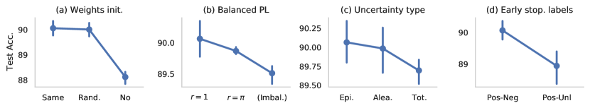
Figure 4: Mean and standard deviation of the test accuracy obtained over five runs by different variations of our PUUPL algorithm: (a) different weight initialization at each iteration, (b) balanced or imbalanced PL selection, (c) type of uncertainty, (d) whether to use PN or PU validation set. Note the different scales on the $y$-axes.

Weight initialization: We confirmed the observation that it is beneficial to re-initialize the weights after each pseudo-labeling step [9], with slightly better performance ($+0.052\%$) achieved when the weights are re-initialized to the same values before every pseudo-labeling iteration (Fig. 4a). We believe this encourages the model to be consistent across pseudo-labeling rounds.

Uncertainty: Ranking predictions by aleatoric performance was almost as good as ranking by epistemic uncertainty ($-0.08\%$), while total uncertainty produced moderately worse rankings ($-0.37\%$, Fig. 4c). An ensemble with only two networks achieved the best performance, while larger ensembles performed worse, and Monte Carlo dropout ($-0.85\%$) was better than ensembles of five ($-1.00\%$) and ten networks ($-1.58\%$).

Early stopping: Finally, performing early stopping on the validation PU loss resulted in worse accuracy ($-1.12\%$) compared to using the accuracy on PN labels (Fig. 4d). Although considerable when compared to the impact of other algorithmic choices, such a performance drop indicates that PUUPL can be used effectively in real-world scenarios when no labeled validation data are available.

pseudo-labeling hyperparameters: Our method was fairly robust to the maximum number $T$ of assigned pseudo-labels and the maximum uncertainty threshold $t_{l}$ for the pseudo-labels, with almost constant performance up to $T=1000$ and $t_{l}=0.1$. The best performance was achieved by the combination having $T=1000$ and $t_{l}=0.05$, but both of these experiments were performed while disabling the other constraint (i.e., setting $T=\inf$ when testing $t_{l}$ and vice-versa). Using only a constraint on $T$ resulted in a reduction of $-0.11\%$, while constraining $t_{l}$ alone resulted in a reduction of $-1.04\%$. The results for $t_{u}$ were less conclusive than for the general trend, possibly because values lower than 0.35 require more than the 15 pseudo-labeling iterations we used for the experiment, and values above 0.4 did not show significant differences.

Moreover, soft pseudo-labels were preferred over hard ones ($+0.75\%$). Contrary to expectation, however, re-assigning all pseudo-labels at every iteration slighly harmed performance ($-0.12\%$); instead, pseudo-labels should be kept fixed after being assigned for the first time. A possible explanation is that fixed pseudo-labels prevent the model’s predictions from drifting too far away from the initial pseudo-labeling towards an incorrect assignment, and thus contribute in mitigating the sort of confirmation bias that frequently plagues pseudo-labeling-based methods. It was also beneficial to assign the same number of positive and negative pseudo-labels compared to keeping the same ratio $\pi$ of positives and negatives found in the whole dataset ($-0.20\%$) or not balancing the selection at all ($-0.55\%$). This prevents the pseudo-labeled set from becoming too imbalanced over time, a natural tendency deriving from the inherent imbalance between positive and unlabeled samples in the training set.

References

- [1] Harotune K Armenian and Abraham M Lilienfeld. The distribution of incubation periods of neoplastic diseases. American journal of epidemiology, 99(2):92–100, 1974.
- [2] Vladimir Gligorijević, P Douglas Renfrew, Tomasz Kosciolek, Julia Koehler Leman, Daniel Berenberg, Tommi Vatanen, Chris Chandler, Bryn C Taylor, Ian M Fisk, Hera Vlamakis, et al. Structure-based protein function prediction using graph convolutional networks. Nature communications, 12(1):1–14, 2021.
- [3] Anthony W. Purcell, Sri H. Ramarathinam, and Nicola Ternette. Mass spectrometry–based identification of MHC-bound peptides for immunopeptidomics. Nat Protoc, 14(6):1687–1707, may 2019.
- [4] Marthinus C Du Plessis, Gang Niu, and Masashi Sugiyama. Analysis of learning from positive and unlabeled data. Advances in neural information processing systems, 27:703–711, 2014.
- [5] Ryuichi Kiryo, Gang Niu, Marthinus C du Plessis, and Masashi Sugiyama. Positive-unlabeled learning with non-negative risk estimator. Advances in Neural Information Processing Systems, 2017.
- [6] Jessa Bekker and Jesse Davis. Learning from positive and unlabeled data: A survey. Machine Learning, 109(4):719–760, 2020.
- [7] Dong-Hyun Lee. Pseudo-label: The simple and efficient semi-supervised learning method for deep neural networks. In Workshop on Challenges in Representation Learning, ICML, volume 3, page 896, 2013.
- [8] Jesper E Van Engelen and Holger H Hoos. A survey on semi-supervised learning. Machine Learning, 109(2):373–440, 2020.
- [9] Eric Arazo, Diego Ortego, P. Albert, N. O’Connor, and Kevin McGuinness. Pseudo-labeling and confirmation bias in deep semi-supervised learning. 2020 International Joint Conference on Neural Networks (IJCNN), pages 1–8, 2020.
- [10] Moloud Abdar, Farhad Pourpanah, Sadiq Hussain, Dana Rezazadegan, Li Liu, Mohammad Ghavamzadeh, Paul Fieguth, Xiaochun Cao, Abbas Khosravi, U Rajendra Acharya, et al. A review of uncertainty quantification in deep learning: Techniques, applications and challenges. Information Fusion, 76:243–297, 2021.
- [11] M. N. Rizve, Kevin Duarte, Y. Rawat, and M. Shah. In defense of pseudo-labeling: An uncertainty-aware pseudo-label selection framework for semi-supervised learning. International Conference on Learning Representations, 2021.
- [12] Bing Liu, Yang Dai, Xiaoli Li, Wee Sun Lee, and Philip S Yu. Building text classifiers using positive and unlabeled examples. In Third IEEE International Conference on Data Mining, pages 179–186. IEEE, 2003.
- [13] Lukas Ruff, Robert Vandermeulen, Nico Goernitz, Lucas Deecke, Shoaib Ahmed Siddiqui, Alexander Binder, Emmanuel Müller, and Marius Kloft. Deep one-class classification. In International conference on machine learning, pages 4393–4402. PMLR, 2018.
- [14] Wenkai Li, Qinghua Guo, and Charles Elkan. A positive and unlabeled learning algorithm for one-class classification of remote-sensing data. IEEE Transactions on geoscience and remote sensing, 49(2):717–725, 2010.
- [15] Yixing Xu, Chang Xu, Chao Xu, and Dacheng Tao. Multi-positive and unlabeled learning. In Proceedings of the Twenty-Sixth International Joint Conference on Artificial Intelligence, pages 3182–3188, 2017.
- [16] Hirotaka Kaji, Hayato Yamaguchi, and Masashi Sugiyama. Multi task learning with positive and unlabeled data and its application to mental state prediction. In 2018 IEEE International Conference on Acoustics, Speech and Signal Processing (ICASSP), pages 2301–2305, 2018.
- [17] Olivier Chapelle, Bernhard Scholkopf, and Alexander Zien. Semi-supervised learning. Cambridge, Massachusettes: The MIT Press View Article, 2009.
- [18] Masahiro Kato, Takeshi Teshima, and Junya Honda. Learning from positive and unlabeled data with a selection bias. In International Conference on Learning Representations, 2019.
- [19] Yu-Guan Hsieh, Gang Niu, and Masashi Sugiyama. Classification from positive, unlabeled and biased negative data. In Kamalika Chaudhuri and Ruslan Salakhutdinov, editors, Proceedings of the 36th International Conference on Machine Learning, volume 97 of Proceedings of Machine Learning Research, pages 2820–2829. PMLR, 09–15 Jun 2019.
- [20] Chuan Luo, Pu Zhao, Chen Chen, Bo Qiao, Chao Du, Hongyu Zhang, Wei Wu, Shaowei Cai, Bing He, Saravanakumar Rajmohan, et al. Pulns: Positive-unlabeled learning with effective negative sample selector. In Proceedings of the AAAI Conference on Artificial Intelligence, volume 35, pages 8784–8792, 2021.
- [21] Guangxin Su, Weitong Chen, and Miao Xu. Positive-unlabeled learning from imbalanced data. In Proceedings of the Thirtieth International Joint Conference on Artificial Intelligence. International Joint Conferences on Artificial Intelligence Organization, aug 2021.
- [22] Hui Chen, Fangqing Liu, Yin Wang, Liyue Zhao, and Hao Wu. A variational approach for learning from positive and unlabeled data. In Advances in Neural Information Processing Systems, pages 14844–14854, 2020.
- [23] Saurabh Garg, Yifan Wu, Alexander J Smola, Sivaraman Balakrishnan, and Zachary Lipton. Mixture proportion estimation and pu learning:a modern approach. In M. Ranzato, A. Beygelzimer, Y. Dauphin, P.S. Liang, and J. Wortman Vaughan, editors, Advances in Neural Information Processing Systems, volume 34, pages 8532–8544. Curran Associates, Inc., 2021.
- [24] Wenpeng Hu, Ran Le, Bing Liu, Feng Ji, Jinwen Ma, Dongyan Zhao, and Rui Yan. Predictive adversarial learning from positive and unlabeled data. Proceedings of the AAAI Conference on Artificial Intelligence, 35(9):7806–7814, May 2021.
- [25] Xuxi Chen, Wuyang Chen, Tianlong Chen, Ye Yuan, Chen Gong, Kewei Chen, and Zhangyang Wang. Self-pu: Self boosted and calibrated positive-unlabeled training. In International Conference on Machine Learning, pages 1510–1519. PMLR, 2020.
- [26] Anish Acharya, Sujay Sanghavi, Li Jing, Bhargav Bhushanam, Dhruv Choudhary, Michael G. Rabbat, and Inderjit S. Dhillon. Positive unlabeled contrastive learning. ArXiv, abs/2206.01206, 2022.
- [27] Yunrui Zhao, Qianqian Xu, Yangbangyan Jiang, Peisong Wen, and Qingming Huang. Dist-pu: Positive-unlabeled learning from a label distribution perspective. In Proceedings of the IEEE/CVF Conference on Computer Vision and Pattern Recognition (CVPR), pages 14461–14470, June 2022.
- [28] Zayd Hammoudeh and Daniel Lowd. Learning from positive and unlabeled data with arbitrary positive shift. In H. Larochelle, M. Ranzato, R. Hadsell, M.F. Balcan, and H. Lin, editors, Advances in Neural Information Processing Systems, volume 33, pages 13088–13099. Curran Associates, Inc., 2020.
- [29] Ahmet Iscen, Giorgos Tolias, Yannis Avrithis, and Ondrej Chum. Label propagation for deep semi-supervised learning. In Proceedings of the IEEE/CVF Conference on Computer Vision and Pattern Recognition, pages 5070–5079, 2019.
- [30] Weiwei Shi, Yihong Gong, Chris Ding, Zhiheng MaXiaoyu Tao, and Nanning Zheng. Transductive semi-supervised deep learning using min-max features. In Proceedings of the European Conference on Computer Vision (ECCV), pages 299–315, 2018.
- [31] Hongyi Zhang, Moustapha Cisse, Yann N. Dauphin, and David Lopez-Paz. Mixup: Beyond empirical risk minimization. International Conference on Learning Representations, 2018.
- [32] Daiki Tanaka, Daiki Ikami, Toshihiko Yamasaki, and Kiyoharu Aizawa. Joint optimization framework for learning with noisy labels. In Proceedings of the IEEE Conference on Computer Vision and Pattern Recognition, pages 5552–5560, 2018.
- [33] Yves Grandvalet and Yoshua Bengio. Semi-supervised learning by entropy minimization. In L. Saul, Y. Weiss, and L. Bottou, editors, Advances in Neural Information Processing Systems, volume 17. MIT Press, 2005.
- [34] Yarin Gal and Zoubin Ghahramani. Dropout as a bayesian approximation: Representing model uncertainty in deep learning. In International Conference on Machine Learning, pages 1050–1059. PMLR, 2016.
- [35] William H Beluch, Tim Genewein, Andreas Nürnberger, and Jan M Köhler. The power of ensembles for active learning in image classification. In Proceedings of the IEEE/CVF Conference on Computer Vision and Pattern Recognition, pages 9368–9377, 2018.
- [36] Balaji Lakshminarayanan, Alexander Pritzel, and Charles Blundell. Simple and scalable predictive uncertainty estimation using deep ensembles. In I. Guyon, U. V. Luxburg, S. Bengio, H. Wallach, R. Fergus, S. Vishwanathan, and R. Garnett, editors, Advances in Neural Information Processing Systems, volume 30. Curran Associates, Inc., 2017.
- [37] Marthinus Christoffel, Gang Niu, and Masashi Sugiyama. Class-prior estimation for learning from positive and unlabeled data. In Asian Conference on Machine Learning, volume 45 of Proceedings of Machine Learning Research, pages 221–236, 2016.
- [38] Aditya Menon, Brendan Van Rooyen, Cheng Soon Ong, and Bob Williamson. Learning from corrupted binary labels via class-probability estimation. In Francis Bach and David Blei, editors, Proceedings of the 32nd International Conference on Machine Learning, volume 37 of Proceedings of Machine Learning Research, pages 125–134, Lille, France, 07–09 Jul 2015. PMLR.
- [39] Eyke Hüllermeier and Willem Waegeman. Aleatoric and epistemic uncertainty in machine learning: An introduction to concepts and methods. Machine Learning, 110(3):457–506, 2021.
- [40] Rafael Müller, Simon Kornblith, and Geoffrey E Hinton. When does label smoothing help? In H. Wallach, H. Larochelle, A. Beygelzimer, F. d'Alché-Buc, E. Fox, and R. Garnett, editors, Advances in Neural Information Processing Systems, volume 32. Curran Associates, Inc., 2019.
- [41] Li Deng. The mnist database of handwritten digit images for machine learning research. IEEE Signal Processing Magazine, 29(6):141–142, 2012.
- [42] Alex Krizhevsky, Geoffrey Hinton, et al. Learning multiple layers of features from tiny images. Citeseer, 2009.
- [43] Han Xiao, Kashif Rasul, and Roland Vollgraf. Fashion-mnist: a novel image dataset for benchmarking machine learning algorithms. arXiv preprint arXiv:1708.07747, 2017.
- [44] Andrew L. Maas, Raymond E. Daly, Peter T. Pham, Dan Huang, Andrew Y. Ng, and Christopher Potts. Learning word vectors for sentiment analysis. In Proceedings of the 49th Annual Meeting of the Association for Computational Linguistics: Human Language Technologies, pages 142–150, Portland, Oregon, USA, June 2011. Association for Computational Linguistics.
- [45] Diederik P. Kingma and Jimmy Ba. Adam: A method for stochastic optimization. CoRR, abs/1412.6980, 2015.
- [46] Lisha Li, Kevin G. Jamieson, Giulia DeSalvo, Afshin Rostamizadeh, and Ameet S. Talwalkar. Hyperband: A novel bandit-based approach to hyperparameter optimization. Journal of Machine Learning Research, 18:185:1–185:52, 2017.
- [47] Shantanu Jain, Martha White, and Predrag Radivojac. Recovering true classifier performance in positive-unlabeled learning. Proceedings of the AAAI Conference on Artificial Intelligence, 31(1), Feb. 2017.
- [48] Edmon Begoli, Tanmoy Bhattacharya, and Dimitri Kusnezov. The need for uncertainty quantification in machine-assisted medical decision making. Nat Mach Intell, 1(1):20–23, jan 2019.
- [49] Rhiannon Michelmore, Matthew Wicker, Luca Laurenti, Luca Cardelli, Yarin Gal, and Marta Kwiatkowska. Uncertainty quantification with statistical guarantees in end-to-end autonomous driving control. In 2020 IEEE International Conference on Robotics and Automation (ICRA), pages 7344–7350. IEEE, 2020.
- [50] Sahil Verma and Julia Rubin. Fairness definitions explained. In Proceedings of the International Workshop on Software Fairness. ACM, may 2018.
- [51] Erik A. Daxberger, Eric T. Nalisnick, James Urquhart Allingham, Javier Antorán, and José Miguel Hernández-Lobato. Bayesian deep learning via subnetwork inference. In ICML, 2021.
- [52] Chuan Guo, Geoff Pleiss, Yu Sun, and Kilian Q. Weinberger. On calibration of modern neural networks. In ICML, 2017.
- [53] Hao Wang and Dit-Yan Yeung. A survey on bayesian deep learning. ACM Comput. Surv., 53(5):1–37, oct 2020.
- [54] Yaniv Ovadia, Emily Fertig, Jie Ren, Zachary Nado, David Sculley, Sebastian Nowozin, Joshua Dillon, Balaji Lakshminarayanan, and Jasper Snoek. Can you trust your model’s uncertainty? evaluating predictive uncertainty under dataset shift. Advances in neural information processing systems, 32, 2019.