Resultant Tools for Parametric Polynomial Systems with Application to Population Models

Abstract.

We are concerned with the problem of decomposing the parameter space of a parametric system of polynomial equations, and possibly some polynomial inequality constraints, with respect to the number of real solutions that the system attains. Previous studies apply a two step approach to this problem, where first the discriminant variety of the system is computed via a Gröbner Basis (GB), and then a Cylindrical Algebraic Decomposition (CAD) of this is produced to give the desired computation.

However, even on some reasonably small applied examples this process is too expensive, with computation of the discriminant variety alone infeasible. In this paper we develop new approaches to build the discriminant variety using resultant methods (the Dixon resultant and a new method using iterated univariate resultants). This reduces the complexity compared to GB and allows for a previous infeasible example to be tackled.

We demonstrate the benefit by giving a symbolic solution to a problem from population dynamics $-$ the analysis of the steady states of three connected populations which exhibit Allee effects $-$ which previously could only be tackled numerically.

1. Introduction

1.1. Problem statement

Let $R=\mathbb{Q}[k_{1},\dots,k_{r}][x_{1},\dots,x_{n}]$ be the ring of polynomials in $n$ variables $x=(x_{1},\dots,x_{n})$ with coefficients coming from the ring of polynomials in $r$ parameters $k=(k_{1},\dots,k_{r})$ with rational coefficients. A system of parametric polynomial equations is defined by a finite set of polynomials $F=\{f_{1},\dots,f_{m}\}\subset R$. For each specification of the parameters $k^{\star}\in\mathbb{R}^{r}$, the solution set to $f_{1}=\dots=f_{m}=0$ will be a subset of $\mathbb{R}^{n}$, i.e. the variety $V(F|_{k=k*})$.

In many applications the concept under study can be modelled by such a parametric system of polynomial equations. It is often the case in such applications that the system of interest has finitely many solutions (for generic choices of the parameters). In such cases one common desire is to know the possible number of solutions and the parameter regions where each of these possible numbers are attained. This is the case for example in chemical reaction network theory (see e.g. (BDEEGGHKRSW20, )) and for the study of population dynamics, which is the application we focus on in this paper.

Thus our problem is to decompose the parameter space for such a system into connected subsets, where the number of solutions to a polynomial system is invariant.

1.2. Decompositions

One potential tool is Cylindrical Algebraic Decomposition (CAD). Invented by Collins in the 1970s (Collins-1975, ), CAD produces a decomposition of an $N$-dimensional real space $\mathbb{R}^{N}$ into connected components (cells) which are semi-algebraic (may be described by a sequence of polynomial constraints). The cells are cylindrical with respect to a given variable ordering: meaning the projections of any two cells onto a lower coordinate space in the same ordering are either equal or disjoint. I.e. the cells stack up in cylinders.

Collins’ original CAD algorithm produced cells on which a set of input polynomials were all sign-invariant (i.e. positive, zero, or negative throughout a given cell). One can then check a single sample point of a cell and infer many properties throughout the cell, such as the truth of any formulae built with the polynomials. The original motivation of Collins was to allow for quantifier elimination over the reals (Collins-1975, ). The common framework of most CAD algorithms involves two stages: first a projection stage to progressively identify polynomials of fewer variables, and then a lifting stage which uses these to build the decomposition.

A sign-invariant decomposition for the polynomials in our input equations would match our requirements, however, it would likely involve far more cells that needed. Since its inception CAD has been developed intensively, with one path of improvements on invariance properties weaker than sign invariance but still sufficient for the problem at hand (Bradford-Davenport-England-McCallum-Wilson-Projection-Doubly-exponential, ; McCallum-1999, ). However, CAD has complexity doubly exponential in $N$ (BD07, ). In the context of our problem $N$ is the total number of indeterminants (i.e. both variables $x$ and parameters $k$), thus doubly exponential in $r+n$. So although CAD is suited to the problem in theory, it is not practical as a tool on its own.

Recall that we want a decomposition of only the parameter space. Thus we may simplify CAD to perform the full projection and terminate lifting once the parameter space alone is decomposed. However, this will still provide a decomposition on which all the defining polynomials of the input equations have invariant sign: something more fine-grained than our requirement of invariance for the number of solutions to the system.

1.3. Contributions and plan of the paper

Hope lies in the combination of CAD with other algebraic approaches. For example, when CAD was used for chemical reaction network analysis in (BDEEGGHKRSW20, ) it was combined with virtual term substitution and lazy real triangularization.

The present state of the art for our problem is a combination of CAD with another tool: the discriminant variety (LR07, ). This is described by polynomials in the parameters and provides the boundaries between the invariant regions we seek. We first compute this and then perform a sign-invarant CAD of only the parameter space with respect to it. We describe this approach in Section 3.

However, this approach has proven infeasible for recent studies of population models. We introduce those models next in Section 2 and then after in Section 4 we summarise those recent attempts which resorted instead to symbolic-numeric methods.

We then describe our new contribution in Section 5, which allows for a purely symbolic solution to this problem. The new approach replaces the Gröbner basis with resultant techniques, less extensive than those used in CAD projection. The symbolic solution to the population model problem is described in Section 6.

2. Population Models $-$ Allee Effect

A well-known population model is logistic growth, where due to a limitation of resources the population can not exceed a certain level. At the beginning when the size of population is small, because of an abundance of resources, the growth of the population is high; but as time passes and the population increases, the amount of available resources per individual decreases and the speed of growth reduces until eventually the population reaches a steady state which is called the carrying capacity of the system (Logistic-population-growth-2020, ).

The Allee effect is a less well-known phenomenon in biology where the population is not only competing for resources, as in logistic growth models, but also has cooperative behaviour which increases the chance of survival. The Allee effect was first described by an American ecologist, Wrder Clyde Allee in the 1930s when he was studying the behaviour of goldfish population (Allee-1932, ).

A strong Allee Effect happens when the population needs to be above a certain amount, called the Allee threshold, to benefit from the cooperative behaviour and be safe from extinction. An Allee effect can be caused by different reasons, e.g. at a low population density the species has difficulty finding mates for reproduction and fertilization (Strong-Allee-example-Fig-trees, ). A strong Allee effect behavior has been observed in various species such as some starfishes (Stong-Allee-effect-example-starfish-1, ; Stong-Allee-effect-example-starfish-2, ) and bacteria (Strong-Allee-effect-example-bacteria, ).

A simple population model with the strong Allee effect is:

$$\frac{dx(t)}{dt}=x(t)\big{(}1-x(t)\big{)}\big{(}x(t)-b\big{)},$$

where $x(t)$ is the population size at time $t$. In this example the carrying capacity is 1 and the Allee threshold is $b$ (where $0<b<1$). From here on we drop the emphasis on $t$ and write $x$ and $\dot{x}$ instead of $x(t)$ and $dx(t)/dt$. The dynamical behavior of a single population with the strong Allee effect is shown in Figure 1. We can easily identify the three steady states by setting the derivative to zero. Two of them are stable, extinction and the carrying capacity, while a third, the Allee threshold, is unstable.

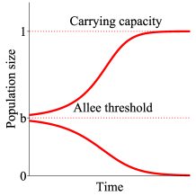
Figure 1. Dynamical behaviour of a single population with the strong Allee effect. If the initial size of the population is below the Allee threshold, the population will eventually become extinct. Otherwise it will survive and increase until reaching the carrying capacity.

Graph which shows an initial population greater than b growing to the carrying capacity; and an initial population less than b declining to zero.

The situation becomes more interesting when several populations of the same species with strong Allee effect are connected. The study of dynamical behavior of connected populations with Allee effects is an ongoing recent research topic (Gyllenberg-Hemminki-Tammaru-1999, ; Knipl-Rost-2014, ; Knipl-Rost-2016, ; Rost-Sadeghimanesh-2021-1, ; Rost-Sadeghimanesh-2021-2, ; Vortkamp-Schreiber-Hastings-Hilker-2020, ). Consider $n$ populations for $n\in\mathbb{N}$ and denote the size of the $i$-th population with $x_{i}$. The simplest scenario is to connect all populations to each other with a complete digraph and assume the same dispersal rate for each path. Let $a$ be the dispersal rate and assume that all populations have the same Allee threshold, $b$. The ordinary differential equation system governing the dynamical behaviour of this model is then as follows (Rost-Sadeghimanesh-2021-1, , Equation (3)):

(2.1) $$\dot{x}_{i}=x_{i}(1-x_{i})(x_{i}-b)-(n-1)ax_{i}+\sum_{\begin{subarray}{c}j=1\\ j\neq i\end{subarray}}^{n}ax_{j},\quad i=1,\dots,n.$$

To study the steady states of this model, one has to obtain the non-negative real solutions to the parametric polynomial system of equations obtained by setting all $\dot{x_{i}}$ equal to zero in system of equations (2.1). Here $a$ and $b$ are the parameters, which may be chosen from $\mathbb{R}_{\geq 0}$, and the $x_{i}$’s are variables. Of most interest is understanding the different parameter regions which give rise to different numbers of steady states, i.e. a problem as defined in Section 1.1.

3. CAD and Discriminant Variety

In this section we describe an approach to tackle the problem introduced in Section 1.1. It is described originally in (LR07, ; Moroz-PhD-thesis, ) and is implemented in Maple as RootFinding[Parametric] (RootFinding-package, ).

3.1. Method and example

The method has two steps: the first consists of finding the possible candidates for the boundaries between different regions where the number of solutions may vary; and the second consists of decomposing the parameter space with respect to these possible boundaries in an algorithmic way. Note that in applications such as in biology one is only interested in open regions. The reason is that in experiments one can not guarantee to fix the parameters to an exact value due to natural perturbations or inevitable small errors in measurement tools. Therefore we will ask this algorithm to only return the open regions in the decomposition.

We illustrate on a simple worked example. Let $R=\mathbb{Q}[b,c][x]$ and $F=\{f\}$ where $f=x^{2}+bx+c$. The parameter space is $\mathbb{R}^{2}$. For every choice of $(b,c)\in\mathbb{R}^{2}$ the set $V(F)$ has finitely many real solutions. For the number of points in $V(F)$ to change, one must vary $(b,c)$ such that they cross a value where a solution gets multiplicity higher than one. This is because to reduce the number of real solutions, two real solutions must collide and leave the real line, and to increase the number of real solutions, two non-real complex solutions must collide and enter the real line. In such situations an additional equation, $df/dx=0$ should hold in addition to $f=0$. So the first step in this algorithm is to find values for $(b,c)$ such that there exists a choice of $x$ that satisfies $f=df/dx=0$.

This is a type of quantifier elimination problem and can be solved using elimination theory via Gröbner Basis (GB) computation. We compute a GB for the ideal generated by $x^{2}+bx+c$ and $2x+b$ with a lexicographic monomial order and considering $x$ greater than $b$ and $c$ in the ring $\mathbb{Q}[b,c,x]$. We then remove the polynomials involving $x$ from the output. The result is the Zariski closure of the set of parameters that we are looking for. In this example we end up with a single polynomial $4c-b^{2}$. This is the discriminant and more generally the output of the process is called the discriminant variety. Figure 2(a) shows $V(4c-b^{2})$.

The second step of the method is to use an open CAD (i.e. a CAD which returns only the cells of full dimension (WBDE14, )) to decompose $\mathbb{R}^{2}$ with respect to this curve. This will produce four open sets for our example, as shown in Figure 2(b). The number of real points in $V(F)$ is invariant in each of these open cells. Therefore now it is enough to pick one sample point from each and solve the system after substituting these values for the parameters of the system and count the number of real solutions. In this example, the cells numbered 1, 2 and 4 have two real solutions and in cell number 3 the system has no real solution. Figure 2(c) shows the result. Here the regions of the same colour indicate the same number of solutions of the system. We acknowledge that the number of solutions on the boundaries of the decomposition (the dashed lines) are not determined by this process, but if desired they could be uncovered by computing the full CAD and testing the additional cells.

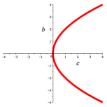
(a)

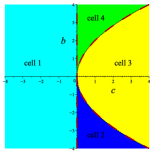
(b)

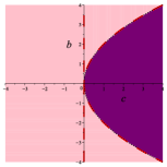
(c)

Figure 2. (a) The discriminant variety of the parametric system $x^{2}+bx+c=0$ when one studies the number of real solutions. (b) The open CAD of the parameter plane with respect to the discriminant variety in (a). (c) The system has two real solutions in the pink coloured region and no real solution in the purple coloured region.

(a) shows a plot of the discriminant variety: a hyperbola; (b) shows a decomposition of the plane into 4 cells relative to this (the region left of the hyperbola and that above below and within it; (c) shows this decomposition coloured according to the number of real solutions with cells merged if they have the same number.

3.2. Restricting to positive solutions

In many applications it is common to care only about the positive solutions to the system (it is not possible to have a population of negative size for example). This means that in addition to our parametric polynomial equations we have inequalities also. Suppose we include $x>0$ along with $f=0$ from our simple example. In this case the discriminant variety has an extra component. Note that the sign of the real solutions may change if by varying the parameters we cross a choice of $(b,c)$ such that a solution to the system becomes zero. So again we have a new quantifier elimination problem. We want to check if there are choices of $(b,c)$ such that there exists $x$ satisfying $f=x=0$. Once again we can solve this using a GB computation to obtain the polynomial $c$.

So in this case the discriminant variety is $V(4c-b^{2})\cup V(c)$, as shown in Figure 3(a). The open CAD gives the same four cells as the previous case. However, previously the line $c=0$ was computed as part of the CAD process while this time it was an explicit input to the system. Testing the sample points we find the system has one positive solution over cell 1, two positive solutions over cell 2, and no positive solutions over cells 3 and 4: as visualised in Figure 3(b).

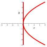
(a)

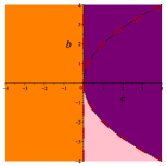
(b)

Figure 3. (a) The discriminant variety of the parametric system $x^{2}+bx+c=0$ when one studies the number of positive real solutions. The open CAD of the parameter plane with respect to this is the same as Figure 2(b). (b) The system has one, two and no positive solutions in the orange, pink and purple coloured regions respectively.

(a) shows a plot of the discriminant variety: a hyperbola and the vertical axis; (b) shows a decomposition of the plane into cells according to the number of positive real solutions.

For a more involved example see the work of (Lichtblau2021, ) which applied the approach to a problem from chemical reaction networks theory.

4. Recent Prior work on our Population Model Application

Recently, in (Rost-Sadeghimanesh-2021-1, ; Rost-Sadeghimanesh-2021-2, ), the problem described in Section 2 was studied using, amongst others, the tools just introduced. The combination of discriminant variety and CAD implemented in Maple’s RootFinding[Parametric] package was used on a normal laptop to successfully study two populations with the strong Allee effect in (Rost-Sadeghimanesh-2021-2, ). However, when attempted for the three population case in (Rost-Sadeghimanesh-2021-1, ) this algorithm did not terminate on a normal laptop before running into memory limitations.

An investigation into the problem identified that the first step of the algorithm, the computation of the discriminant variety, was infeasible on its own. Note that this computation usually relies on GB techniques. Unfortunately in this case the GB computation needed to compute the discriminant variety is not feasible on a normal computer. To overcome this problem, in (Rost-Sadeghimanesh-2021-1, ), a combination of this algebraic method, CAD with respect to the discriminant variety, with a numerical sampling approach was developed, to build an approximation of the requested decomposition of the parameter space. We note a similar approach for studying chemical reaction networks in the work of (EEGRSW17, ).

The numeric-algebraic algorithm in (Rost-Sadeghimanesh-2021-1, ) consists of two steps. The first step is to fix a value of one of the parameters and use the algebraic algorithm with one parameter less. This gives the intersection of the discriminant variety with the hyperplanes defined by the fixing of the other parameter. Figure 4(a) shows the result of this step for 11 equally distanced values of $b$ between and including 0 and 1/2. The next step is using a numeric search and again the algebraic algorithm with one parameter fixed, to find regions where the behavior of the intersection of the discriminant variety with the horizontal lines changes. This step finds two regions (Rost-Sadeghimanesh-2021-1, , Figure 2) shown in Figures 4(b) and 4(c). The final output of this algorithm is (Rost-Sadeghimanesh-2021-1, , Figure 3) shown in Figures 4(d) and 4(e) which guarantees the behavior of the system up to precision chosen in the numeric-algebraic algorithm, in this case 7 digits after the decimal point.

The method does not guarantee that there is no smaller region with different behaviour that may have been missed. For increased confidence the user could re-run the algorithm with a higher precision requested. However, it is not possible to achieve full certainty and so a symbolic verification of the results is still desired.

Figure 4(e) showed a surprising feature of this analysis: it was expected that when increasing the dispersal rate the number of steady states of the network should monotonically decrease, however, the zoomed in region shows there is a possibility to temporary increase the number of steady states when increasing the dispersal rate, for some choices of the Allee threshold.

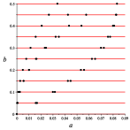
(a)

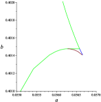
(b)

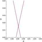
(c)

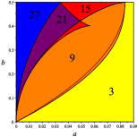
(d)

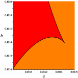
(e)

Figure 4. Figures 4(b), 4(c), 4(d) and 4(e) are taken from (Rost-Sadeghimanesh-2021-1, , Figures 2 and 3). They demonstrate the idea behind the numeric-algebraic algorithm developed in (Rost-Sadeghimanesh-2021-1, ) and the result of its implementation on the three populations with strong Allee effect example. (a) The first step is to find the intersection of the discriminant variety with several hyperplanes defined by fixing a value of one of the parameters, in this case the red color horizontal lines. (b-c) The second step is to run a numeric search to find where the number of intersection points in the previous step change. (d) The final output of the algorithm for the three populations example. (e) Enlargement of a tiny region from part (d) related to the part (b).

As per the caption. The enlarged region shows the region with 15 solutions to be non-convex.

5. New Approaches using Resultants

We now report on some purely algebraic approaches to our problem, which are sufficient to tackle the three population case, and do not use GB to compute the discriminant variety. These algebraic approaches instead use the theory of resultants. The ideas were motivated by the improved CAD performance available when the input contains equational constraints (EBD20, ), but are developed here outside of the CAD context allowing for more simplicity of presentation and greater savings.

5.1. Using a single univariate resultant

We start by considering the simplest use of a resultant. Recall the problem introduced in Section 1.1. In the case where $n=1$ and $m=2$, an alternative to Gröbner basis for the elimination of variable $x_{1}$ to get polynomials only involving parameters is to use a resultant.

We denote the resultant of $f_{1}$ and $f_{2}$ with respect to $x_{1}$ by $g={\rm res}(f_{1},f_{2},x_{1})$. The resultant is a polynomial expression in which $x_{1}$ has been eliminated, and which is equal to zero if and only if the polynomials $f_{1}$ and $f_{2}$ have a common root. It may be calculated as the determinant of the Sylvester Matrix of the two polynomials (a square matrix of size the sum of the degrees in $x_{1}$ of the polynomials, formed from the coefficients of the powers of $x_{1}$).

Note that $V(g)$ contains the discriminant variety, but also possibly more components. Thus an open CAD of the parameter space with respect to $V(g)$ provides the key information that the approach in Section 3 provides.

For the simple example in Section 3.1 we have one variable $x$ and two polynomials $f$ and $f^{\prime}$, the resultant of these two polynomials with respect to $x$ is the following.

$${\rm res}(f,f^{\prime},x)=\begin{vmatrix}1&2&0\\ b&b&2\\ c&0&b\end{vmatrix}=-(b^{2}-4c).$$

I.e. the same polynomial that we found by the Gröbner basis, up to a sign. For the extra part of the discriminant variety of Section 3.2, again we have one variable $x$ and two polynomials $f$ and $x$, the corresponding resultant is the following.

$${\rm res}(f,f^{\prime},x)=\begin{vmatrix}1&1&0\\ b&0&1\\ c&0&0\end{vmatrix}=c.$$

This is again the same polynomial computed by Gröbner basis approach. Therefore for this simple example, replacing the Gröbner basis computation with resultants did not add any extra curve to the discriminant variety.

The question now is what about the case of having more than two polynomials and more than one variable? There are several generalizations of resultants to multi-polynomial cases such as the multipolynomial resultant for $n$ polynomials in $n$ variables using homogenization, or Waerden’s $u$-resultant (see (Cox_Using_Algebraic_Geometry, , Chapter 3)), or the Dixon resultant for $n+1$ polynomials in $n$ variables which will be discussed in Section 5.2. In the applications of our interest, such as population dynamics and Chemical Reaction Network theory, we always have $n$ equations in $n$ variables and an extra polynomial coming from determinant of the Jacobian matrix or positivity constraints etc. Therefore the Dixon resultant is a suitable generalization to try.

5.2. Using the multivariate Dixon resultant

The Dixon resultant is named after Arthur Lee Dixon, a British mathematician who extended the Bezout-Cayley method of computing the simple resultant for computing resultant of three polynomials in two variables (Chtcherba-Kapur-Minimair-2005, ; Dixon-1909, ). It uses only one determinant to produce a polynomial only involving parameters for a system of $n+1$ equations in $n$ variables that vanishes whenever the system has a solution. Therefore if we denote the Dixon resultant of the system $F$ of the problem statement in Section 1.1 by $g$, then $V(g)$ contains the discriminant variety. To see a simple explanation of all the steps of computing the Dixon resultant see (Minimair_DR_package, , Section 2.1). Here we do not explain the general algorithm, but only show the computations for the simple example of Section 3.1.

Define an auxiliary variable $\bar{x}$ and consider the following matrix.

$$M_{1}=\begin{bmatrix}x^{2}+bx+c&2x+b\\ \bar{x}^{2}+b\bar{x}+c&2\bar{x}+b\end{bmatrix}.$$

The Dixon polynomial is defined as $\det(M_{1})/(x-\bar{x})$, denoting it by $p$, we have $p=2x\bar{x}+b(x+\bar{x})+b^{2}-2c$. Then we have to solve the linear system of equations created by considering:

$$\begin{bmatrix}\bar{x}&1\end{bmatrix}\begin{bmatrix}a_{11}&a_{12}\\ a_{21}&a_{22}\end{bmatrix}\begin{bmatrix}x\\ 1\end{bmatrix}=p.$$

Solving gives us the Dixon matrix,

$$M_{2}=\begin{bmatrix}2&b\\ b&b^{2}-2c\end{bmatrix}.$$

Now the Dixon resultant is the determinant of a maximal-rank submatrix of $M_{2}$ which is $M_{2}$ itself. We get $\det(M_{2})=b^{2}-4c$ as expected.

Thus the first part of the algorithm in Section 3 may be replaced by the Dixon resultant. There are several implementations of the Dixon resultant, for example based on how to find the maximal-rank submatrix or how to compute the determinants. One implementation can be found in the computer algebra system Fermat (Lewis-2004, ), and another implementation is a Maple package called DR (Minimair_DR_package, ).

A complexity analysis on construction of the Dixon resultant matrix is given in (Qin_Dixon_res_complexity, , Theorem 3.1) which is of order of $\mathcal{O}(n!^{3}\mathfrak{m}^{4n})$ where $\mathfrak{m}$ is the maximal univariate degree of the polynomials in $F$ in each of its variables. This complexity is somewhere between singly exponential and doubly exponential; lower than the worst case complexity of Gröbner basis computation which is doubly exponential in $n+r$ (with the Gröbner basis computation is in the ring $\mathbb{Q}[k_{1},\dots,k_{r},x_{1},\dots,x_{n}]$) (Mayr-Meyer-1982, ; Mayr-Ritscher-2013, ).

5.3. Using a chain of univariate resultants

We next consider an alternative to the Dixon resultant based on iterated use of the univariate resultant from Section 5.1.

Let $f_{1}$ and $f_{2}$ be two polynomials in $N$ variables, $x_{1},\dots,x_{N}$. Then by Theorem 8 of (Cox_Ideals_Varieties_and_Algorithms, , Chapter 3), if the degrees of $f_{1}$ and $f_{2}$ in $x_{N}$ are positive, we have that

$$V(f_{1},f_{2})\cap\mathbb{R}^{N-1}\subseteq V({\rm res}(f_{1},f_{2},x_{N})).$$

In other words, $V({\rm res}(f_{1},f_{2},x_{N}))$ contains the projection of the set of common solutions of $f_{1}$ and $f_{2}$ into their first $N-1$ coordinates. On the other hand if the degree of either of these two polynomials in $x_{N}$ is not positive, then clearly $V(f_{1},f_{2})\cap\mathbb{R}^{N-1}$ is a subset of solution set of the one (or both) which does not involve $x_{N}$ as polynomials in $N-1$ variables.

Now assume $F$ contains $m$ polynomials in $N$ variables, where $m>N$. In the case where the degree in $x$ of $f_{1}$, or $f_{2}$, or both is not positive, we will redefine ${\rm res}(f_{1},f_{2},x_{N})$ to be respectively $f_{1}$, $f_{2}$ or $f_{1}f_{2}$. This gives different results to the Sylvester determinant (which would be a power of the polynomial for the first two and a constant for the latter). We now have that

$$V(F)\cap\mathbb{R}^{N-1} =\bigcap_{i=2}^{m}(V(f_{1},f_{i})\cap\mathbb{R}^{N-1})$$

$$\subseteq\bigcap_{i=2}^{m}V({\rm res}(f_{1},f_{i},x_{N})).$$

Taking this set of resultants gives us $m-1$ polynomials in $N-1$ variables.

This gives us a route to use iterated univariate resultants to solve our problem. Let us return to the parametric polynomial ring in Section 1.1, with $n$ variables and $r$ parameters. Now let $m$ be the number of polynomials in the original system of equations plus the extra polynomials needed to study the discriminant variety. If $m>n$, then repeating the above process iteratively after $n$ steps, one gets $m-n$ polynomials involving only parameters. We denote these polynomials by $g_{i}$, $i=1,\dots,m-n$. Then $V(g_{1},\dots,g_{m-n})$ contains the discriminant variety.

5.4. Degree drops and constant evaluations

Note that when taking the resultant ${\rm res}(f_{1},f_{2},x_{i})$ it is possible that the polynomial produced does not have positive degree in $x_{i-1}$. In this case, the resultants taken in the subsequent stage will be evaluated according to the modified resultant definition above. This has the effect of passing the information down to the relevant level.

Let us now consider what happens when a resultant evaluates to zero. This means that the two input polynomials have a common root everywhere. This would happen if the two polynomials have a common factor. If in the above process all $m$ polynomials share a common factor we can return $0$ as the defining polynomial of the projection. But if only some of them share a common factor, then we will continue the process in two separate branches. We explain this by means of a simple example system with $f_{1}=h_{0}h_{1}$ and $f_{2}=h_{0}h_{2}$ where $h_{1}$ and $h_{2}$ are relatively prime and $h_{0}$ is not a factor of $f_{i}$ for $i=3,\dots,m$. We have that

$$V(F)\cap\mathbb{R}^{N-1}=\big{(}V(h_{1},h_{2},f_{3},\dots,f_{m})\cup V(h_{0},f_{3},\dots,f_{m})\big{)}\cap\mathbb{R}^{N-1}\\ =\big{(}V(h_{1},h_{2},f_{3},\dots,f_{m})\cap\mathbb{R}^{N-1}\big{)}\bigcup\big{(}V(h_{0},f_{3},\dots,f_{m})\cap\mathbb{R}^{N-1}\big{)}.$$

Thus one can apply the former process on these two branches and at the end take union of the final output sets of polynomials where the variables are eliminated.

If a resultant evaluates to a non-zero constant then it means that the two input polynomials can never share a common root. Should this happen it means there is no solution to the problem and the algorithm can terminate. Although if we have branched as above then we could only terminate that branch.

5.5. Efficiencies from factorisation

Using the fact that ${\rm res}(p_{1}p_{2},p_{3},x)={\rm res}(p_{1},p_{3},x){\rm res}(p_{2},p_{3},x)$ one can modify the above process so that the size of the Sylvester Matrix determinants needed to be computed gets smaller. Suppose we are computing the resultant of two polynomials $p=\prod_{i=1}^{s}p_{i}^{\alpha_{i}}$ and $q=\prod_{i=1}^{t}q_{i}^{\beta_{i}}$, where $p_{i}$ and $q_{j}$ are irreducible factors of $p$ and $q$. Then instead of a single determinant of size $\sum_{i=1}^{s}\alpha_{i}{\rm degree}(p_{i})+\sum_{i=1}^{t}\beta_{i}{\rm degree}(q_{i})$ one can use $st$ determinants of the sizes ${\rm degree}(p_{i})+{\rm degree}(q_{j})$.

Note that this should mean less computation resources. For example, consider the simplified situation where $\hat{p}$ is the maximum degree of any factor, $\hat{s}$ is the maximum number of factors and there are no repeated factors (i.e. $\alpha_{i}=\beta_{i}=1$ for all $i$). Then we are comparing a single determinant of size $2\hat{s}\hat{p}$ with $\hat{s}^{2}$ determinants of size $2\hat{p}$. Calculating the determinant with cost $\mathcal{O}(n)^{3}$ for matrix of size $n$ means we save a factor of $\hat{s}$. Such a saving is repeated at each stage in our chain of univariate resultant computation.

5.6. Algorithm with simple chain of resultants

Following this analysis we implemented an algorithm in Maple called ResChainSimple (Algorithm 1). The algorithm takes a list of polynomials and eliminates variables to produce a set of polynomials; the union of whose varieties has the projection as a subset.

The master list $L$ contains sublists, denoted $B_{k}$ for each of the different branches in the analysis: we start with only one branch in the initialisation. Each branch contains a set of polynomials, each represented by a list, $P_{j}$ containing their irreducible factors. The outer loop (for loop on $i$) concerns the levels of projection. At each level the while loop processes one branch at a time (noting that an iteration of this loop can create further branches in $L$ to process).

So long as a branch contains more than one polynomial with a variable we enter the for loop on $j$ which takes the resultants of the factors of the first polynomial with the others. Should a common factor be found then an additional branch is created as discussed.

If a branch contains only one polynomial (list of factors) involving a variable, then the algorithm terminates and returns a single polynomial, 0. This trivially meets the specification (in the sense that $V(0)$ is the whole space and thus has the projection as a subset) but of course is not useful. This output indicates that the algorithm cannot use resultants to eliminate all the variables, and the user would be advised to seek a different approach. We note that triggering this case terminates not just the branch but the whole algorithm (continuing the other branches would be pointless since the union of their output with $V(0)$ would simply be $V(0)$). We expect that progress can be made on such cases in future work.

1 Function ResChainSimple($F$, $x=(x_{1},\dots,x_{n})$):

       In : $F$ is a list of $m$ polynomials and $x$ is a tuple of $n$ variables. The polynomials are defined in the $n$ variables and an additional $r$ parameters.

       Out : $S$, a set of irreducible polynomials none of which involve the variables in $x$. We have that the projection of $V(F)$ as a subset of $\mathbb{R}^{r+n}$ into $\mathbb{R}^{r}$, is subset of $\cup_{p\in S}V(p)$.

2       initialization: Denote the set of irreducible factors of the $i$th element of $F$ with $P_{i}$ for $i=1,\dots,m$. Let $B_{1}=[P_{1},\dots,P_{m}]$, and $L=[B_{1}]$. I.e. there is only one branch at the start of the algorithm;

3       for $i$ from $n$ by $-1$ to $1$ do

4             Let $L^{\prime}=[\;]$;

5             while $L\neq[\;]$ do

6                   Pick up a branch from $L$, denote it by $B$;

7                   Remove $B$ from $L$;

8                   if $B$ contains only one list then

9                         Let $P$ denote the only member of $B$;

10                         if Any polynomial in $P$ contains $x_{i}$ then

11                               return $[0]$;

12                         else

13                               Append $B$ to $L^{\prime}$;

14                              

15                         end if

16                        

17                   else

18                         Let $B=[P_{1},\dots,P_{m}]$;

19                         for $j$ from $1$ by $1$ to $m-1$ do

20                               $P_{j}^{\prime}=[\;]$;

21                               for $f$ in $P_{1}$ do

22                                     for $g$ in $P_{j+1}$ do

23                                           if $f=g$ then

24                                                 Set $B^{\prime}$ to the list found by removing all $P_{i}$ with $f$ from $B$, and prepend a list $[f]$ to its start;

25                                                 Append $B^{\prime}$ to $L$;

26                                                

27                                           else

28                                                 Append irreducible factors of ${\rm res}(f,g,x_{i})$ to $P_{j}^{\prime}$;

29                                                

30                                           end if

31                                          

32                                     end for

33                                    

34                               end for

35                              

36                         end for

37                        Append $[P_{1}^{\prime},\dots,P_{m-1}^{\prime}]$ to $L^{\prime}$;

38                        

39                   end if

40                  

41             end while

42            Replace $L$ with $L^{\prime}$;

43            

44       end for

45      Let $S$ be the union of sets in all branches in $L$;

46       return $S$;

47      

48

End Function

Algorithm 1 Simple approach to use iterated univariate resultants to eliminate variables from equations.

Consider the case where there is no branching because of polynomials sharing a common factor. First suppose that $m=n+1$. Then we only have one branch in each step and the factors of the $j$th polynomial in any step of the iteration are resultants of the factors of the first polynomial and factors of the $(j+1)$-th polynomial in the step before. Finally the last step has only one polynomial and its solution set is the union of solution sets of its factors.

Next suppose $m>n+1$. Then in the last step we have $m-n$ polynomials and the projection is the intersection of the solution set of each of these $m-n$ polynomials. But this intersection set is still a subset of the union of solution sets of factors of all of the $m-n$ polynomials, and as the final output the algorithm just returns the set of all factors of the polynomials in the last step.

In the case where $m<n$, the algorithm will most likely end up with a branch with a single polynomial involving a variable thus returning $0$. This is not certain, and it might be the case that some variables are not present or get eliminated in the projection steps of the other variables such that the algorithm ends up finding the projection even though the number of polynomials is not more than the number of variables.

If branching due to common factors occurs then we can no longer conclude a successful output just because $m\geq n+1$. The branches created have fewer polynomials and so this increases the likelihood of hitting the case where we return $0$. If all branches avoid this case then the final output is the union of the output for each branch.

Note that this algorithm is sensitive to the order of the variables in $x$ (and likewise the open CAD to follow will be sensitive to the order of the parameters). As with CAD more generally, we expect this choice of order may have a significant affect.

Further, Algorithm 1 is sensitive to the order of the polynomials which appear in $F$: it is clear from the algorithm that the first polynomial is treated specially, but note that the order of subsequent polynomials will effect which polynomials are positioned first in subsequent levels, and so has an effect also. Heuristic choices for both of these orderings are a potential topic for further study.

5.7. Algorithm with branching resultant chains

It should not be surprising that Algorithm 1 can potentially generate many extra components that are not part of the discriminant variety. Consider the situation where we have three polynomials $f$, $g$ and $h$ and where $f$ can be factored to $f_{1}f_{2}$. One step of the ResChainSimple algorithm will generate two lists. The first one contains ${\rm res}(f_{1},g,x_{N})$ and ${\rm res}(f_{2},g,x_{N})$, and the second one consists of ${\rm res}(f_{1},h,x_{N})$ and ${\rm res}(f_{2},h,x_{N})$. Then in the second step it creates a list containing four resultants in which we can encounter cases such as

$${\rm res}\Big{(}{\rm res}(f_{1},g,x_{N}),{\rm res}(f_{2},h,x_{N}),x_{N-1}\Big{)}.$$

This will produce an extra component because this is encoding $V(f_{1},g)\cap V(f_{2},h)$ but we do not need $f_{1}$ and $f_{2}$ to both necessarily vanish as they are factors of the same polynomial of the input system $f=f_{1}f_{2}$. We only need $f=0$ which means $f_{1}=0$ or $f_{2}=0$. A condition on parameters for when both vanish together is not a mandatory condition to have $f=g=h=0$.

To avoid computing these extra resultants we modify Algorithm 1 to use a further branching idea. This time, for each factor of the first polynomial in a branch, we create a new branch for the next step and inside put resultants of that factor with factors of the other polynomials in the lists of that branch. We implemented this algorithm in Maple and called it ResChainBranching. This algorithm is the same as Algorithm 1 with lines $17-30$ replaced with the lines in Algorithm 2. In comparison with ResChainSimple, it avoids computing some unnecessary resultants, at the expense of having more branches to keep track of.

1 for $f$ in $P_{1}$ do

2       Let $B^{\prime}=[\;]$;

3       for $j$ from $1$ by $1$ to $m-1$ do

4             Let $P_{j}^{\prime}=[\;]$;

5             for $g$ in $P_{j+1}$ do

6                   if $f=g$ then

7                         Let $B^{\prime\prime}$ be a list resulted by removing all $P_{i}$ containing $f$ and adding the list $[f]$ at its beginning;

8                         Append $B^{\prime\prime}$ to $L$;

9                        

10                   else

11                         Append all irreducible factors of ${\rm res}(f,g,x_{i})$ to $P_{j}^{\prime}$;

12                        

13                   end if

14                  

15             end for

16            Append $P_{j}^{\prime}$ to $B^{\prime}$;

17            

18       end for

19      

20 end for

21Append $B^{\prime}$ to $L^{\prime}$;

Algorithm 2 A modified version of Algorithm 1 such that some of the extra resultant computations are avoided can be obtained by replacing the lines $17-30$ of Algorithm 1 with the above lines.

5.8. Example comparing ResChainSimple and ResChainBranching

Consider the following simple system of parametric equations of three polynomials, two variables, $x$ and $y$, and a single parameter $a$.

$$(x^{2}+y^{2}-1)(y-x^{2})\;=\;x^{3}+x^{2}-y^{2}\;=\;y-a.$$

To find conditions on $a$ for which this system has a solution we must eliminate the two variables.

The ResChainSimple algorithm gives us the 5 polynomials in the set below.

$$\{a,a+1,a-1,a^{2}-3a+1,a^{4}+a^{2}-1\}.$$

However, the ResChainBranching algorithm gives us only three of them, excluding $a+1$ and $a-1$. Using elimination theory via Gröbner basis computation we get a single polynomial which has three irreducible factors in the result of ResChainBranching which shows in this case ResChainBranching did not produce an extra component, while ResChainSimple produced two extra components because of the extra resultants.

5.9. Potential for further optimisation

Although Algorithm 2 can avoid some of the unnecessary components provided by Algorithm 1, it is not guaranteed to produce a minimal number.

Consider the situation where we have four polynomials $f$, $g$, $h$ and $p$ where $g$ and $h$ can be factored respectively to $g_{0}q$ and $h_{0}q$. The first step of ResChainBranching generates a single branch with three polynomials.

$${\rm res}(f,g_{0},x_{N})\cdot{\rm res}(f,q,x_{N}),\quad{\rm res}(f,h_{0},x_{N})\cdot{\rm res}(f,q,x_{N}),$$

$${\rm res}(f,p,x_{N}).$$

The first and the second polynomials have a common factor, ${\rm res}(f,q,x_{N})$, so the algorithm creates a new branch when encountering the request for resultant of this repeated factor from the two polynomials. But it still computes two unnecessary resultants in the old branch shown below.

$${\rm res}\Big{(}{\rm res}(f,g_{0},x_{N}),{\rm res}(f,q,x_{N}),x_{N-1}\Big{)},$$

$${\rm res}\Big{(}{\rm res}(f,q,x_{N}),{\rm res}(f,h_{0},x_{N}),x_{N-1}\Big{)}.$$

It could instead simplify the initial inputs to avoid computing these two extra resultants using the following.

$$V(f,g,h,p)\cap\mathbb{R}^{N-2}=\big{(}V(f,g_{0},h_{0},p)\cup V(f,q,p)\big{)}\cap\mathbb{R}^{N-2}\\ =\big{(}V(f,g_{0},h_{0},p)\cap\mathbb{R}^{N-2}\big{)}\bigcup\big{(}V(f,q,p)\cap\mathbb{R}^{N-2}\big{)}$$

We will leave the quest for finding the most optimized version of ResChain algorithms for a future work. We finish this section by presenting an example where the above scenario actually happens.

Example

Consider the following simple system of parametric equations of four polynomials, two variables, $x$ and $y$, and three parameters $a$, $b$ and $c$. To find conditions on the parameters for which this system has a solution we must eliminate the two variables.

$$x^{2}+y^{2}-1\;=\;(x^{2}-y^{2})(x-c)\;=\;(y-x^{2}+a)(x-c)\;=\;y-b.$$

The ResChainBranching algorithm returns five polynomials:

$$\Big{\{}c^{2}-\tfrac{1}{2},a^{2}-a-\tfrac{1}{4},b^{2}-\tfrac{1}{2},c^{4}-2ac^{2}+a^{2}+c^{2}-1,b^{2}+c^{2}-1\Big{\}}.$$

Using the alternative simplified input we get only three of the above polynomials. The two polynomials that we do not get are exactly the two resultants mentioned above and are the first and the last polynomials above. To check the validity of the answer, i.e. that the discriminant variety is still a subset of the union of solution set of only the three polynomials in the alternative approach, we used elimination via Gröbner basis computation. The result is the union of $V(b^{2}+c^{2}-1)$ and two lines defined by $b^{2}-\frac{1}{2}=a+b-\frac{1}{2}=0$ which are included in $V(a^{2}-a-\frac{1}{4})\cup V(b^{2}-\frac{1}{2})$. This shows indeed two polynomials of the result of ResChainBranching are unnecessary output for this example.

6. Application of New Approach to Population Model Application

Consider System (2.1) with $n=3$ and denote the polynomials on the right by $f_{i}$, $i=1,2,3$. Let $d$ be the determinant of the Jacobian matrix of $f=(f_{1},f_{2},f_{3})$ with respect to $x=(x_{1},x_{2},x_{3})$. Then the ideal associated with the discriminant variety of this system is $\langle f_{1},f_{2},f_{3},d\rangle\cap\mathbb{R}[a,b].$ Recall from Section 4 that we could not before study this symbolically when computing the discriminant variety with a Gröbner basis, and thus relied on a symbolic-numeric analysis instead.

Now, instead of using GB to find a basis for this elimination ideal, we may compute the Dixon resultant of the polynomial set $\{f_{1},f_{2},f_{3},d\}$ with respect to the variables $x$. It took less than 7 minutes on our laptop and the result is the polynomial in (6.1) with 8 irreducible factors, two of which have no solutions in the positive orthant, namely $3a+b$ and $2a+b$.

(6.1) $$\begin{array}[]{l}42391158275216203514294433201b^{2}(3a+b)^{8}(2a+b)^{24}(4a\,b^{4}-\\ 36a^{2}b^{2}-8a\,b^{3}-b^{4}+108a^{3}+36a^{2}b+12a\,b^{2}+2b^{3}-36a^{2}-8ab\\ -b^{2}+4a)^{9}(256a^{4}b^{10}-32a^{2}b^{12}-6144a^{5}b^{8}-1280a^{4}b^{9}+\\ 768a^{3}b^{10}+192a^{2}b^{11}+12a\,b^{12}+54784a^{6}b^{6}+24576a^{5}b^{7}-\\ 4416a^{4}b^{8}-3840a^{3}b^{9}-776a^{2}b^{10}-72a\,b^{11}-b^{12}-165888a^{7}b^{4}-\\ 164352a^{6}b^{5}-16512a^{5}b^{6}+25344a^{4}b^{7}+10848a^{3}b^{8}+2120a^{2}b^{9}+\\ 204a\,b^{10}+6b^{11}-248832a^{8}b^{2}+331776a^{7}b^{3}+207744a^{6}b^{4}-\\ 36480a^{5}b^{5}-54528a^{4}b^{6}-20352a^{3}b^{7}-3800a^{2}b^{8}-360a\,b^{9}-\\ 15b^{10}+2239488a^{9}+248832a^{8}b-497664a^{7}b^{2}-141568a^{6}b^{3}+\\ 62976a^{5}b^{4}+69504a^{4}b^{5}+25152a^{3}b^{6}+4592a^{2}b^{7}+432a\,b^{8}+20b^{9}\\ -248832a^{8}+331776a^{7}b+207744a^{6}b^{2}-36480a^{5}b^{3}-54528a^{4}b^{4}\\ -20352a^{3}b^{5}-3800a^{2}b^{6}-360a\,b^{7}-15b^{8}-165888a^{7}-\\ 164352a^{6}b-16512a^{5}b^{2}+25344a^{4}b^{3}+10848a^{3}b^{4}+2120a^{2}b^{5}+\\ 204a\,b^{6}+6b^{7}+54784a^{6}+24576a^{5}b-4416a^{4}b^{2}-3840a^{3}b^{3}-\\ 776a^{2}b^{4}-72a\,b^{5}-b^{6}-6144a^{5}-1280a^{4}b+768a^{3}b^{2}+192a^{2}b^{3}+\\ 12a\,b^{4}+256a^{4}-32a^{2}b^{2})^{3}(3a+1-b)^{8}(b^{2}+3a-b)^{8}(b-1)^{2}\end{array}$$

A large polynomial.

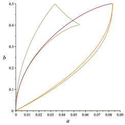
(a)

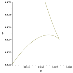
(b)

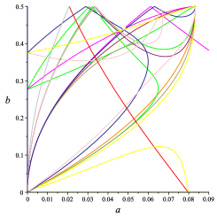
(c)

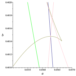
(d)

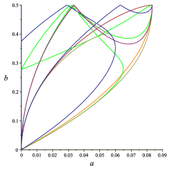
(e)

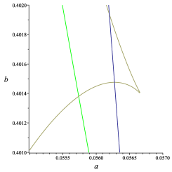
(f)

Figure 5. Graph of the product of the polynomials obtained from eliminating variables $x_{1}$, $x_{2}$ and $x_{3}$ from the system made by $\{f_{1},f_{2},f_{3},d\}$ using resultant techniques instead of Gröbner basis computation. The figures in the left column show the region $[0,0.5]\times[0,\infty)$, and the figures in the right column are zoomed area of their left figures in the region $[0.055,0.057]\times[0.401,0.402]$. The first, second and third rows are obtained by the Dixon resultant, simple chain of resultants (ResChainSimple), and a modified chain of resultants (ResChainBranching) respectively.

As per the caption. As the rows go down he number of curve segments plotted decreases markedly.

Figure 5(a) shows the plot of the solution set of the polynomial found by the Dixon resultant. It is the exact Discriminant variety approximated by the symbolic-numeric approach in Section 4. The interesting region where the number of solutions could temporary increase is related to the solution set of the largest factor of this polynomial. Figure 5(b) shows the zoomed version of this curve at this interesting region. Having only the boundaries that we found by the symbolic-numeric approach in the result of elimination via the Dixon resultant also proves that the result of the Dixon resultant does not contain any extra component in this example, and the result of the symbolic-numeric approach was complete and the behavior of the system was indeed completely classified.

We also applied our two algorithms of a simple chain of iterated univariate resultants and the chain of resultants with branching. The former takes about half of a second and the latter version takes about 5 milliseconds. They are both much faster than the Dixon resultant, but they include extra unnecessary components in the output. The simple version returns 16 irreducible components and the modified one returns 11 components. The set of irreducible factors in the Dixon resultant is a subset of the set of irreducible polynomials in the ResChainBranching, and the latter is a subset of the set of irreducible polynomials in the result of ResChainSimple. Figures 5(c)$-$5(f) show the plot of solution sets of the product of the polynomials in the output of these two methods. We colored each of the 16 components of the result of the simple method with a different color and we used the same color for the 11 (and 8) curves remaining in the result of the modified version (and the Dixon resultant) for a better comparison. The largest polynomial in the output of both resultant chain approaches has 153 terms and total degree of 21. The largest factor of the result of the Dixon resultant has 72 terms and the total degree of 14.

The new approaches can all produce information on the discriminant variety which was infeasible using GB. There is a trade-off between the speed of computation and the presence of redundant components in the output. Depending on the relative sizes of the variable and parameter spaces one approach may be preferred over the other. We note that an open CAD with respect to the union of the polynomials in the output of ResChainBranching (including the unnecessary ones) finishes in about 2 minutes. However, the CAD computation for ResChainSimple output did not terminate after an hour.

So we have tackled the previously intractable 3-population case; and a natural question is whether these approaches are sufficient for the 4-population case? The Dixon resultant computation for four connected populations did not terminate after four hours on our laptop, while the two ResChain algorithms both encounter a branch with single polynomial and so return $0$. Thus further research is needed to progress in this case.

7. Conclusion

In this paper we introduced new methods to decompose the parameter space into regions where a parametric system of polynomial equations has different numbers of solutions. The prior state of the art has had worst case doubly exponential complexity in both its first and second parts, whereas the new algorithm reduces the doubly exponential growth in the number of polynomials in the first part; to somewhat between singly and doubly exponential. The benefits of the new approaches were validated through the symbolic solution of a real world example in a few minutes which was infeasible for the prior approach, showing that the observations in (Rost-Sadeghimanesh-2021-1, ) found by a symbolic-numeric algorithm were indeed a complete classification of the dynamical behaviour of the model.

To tackle larger examples, one option would be to combine the new symbolic approaches with numerical sampling, as was done in (Rost-Sadeghimanesh-2021-1, ). We intend to explore the limit of the new algorithms in hybrid as future work. There is also hope to improve the symbolic methods as future work: both by the use of additional projection technology to deal with the case where a branch has a single polynomial; and by further optimisations to remove the remaining redundancies in the output of Algorithm 2.

Data Access Statement

The code and data described in this paper is openly available from this URL: https://doi.org/10.5281/zenodo.5902594

Acknowledgements

The authors acknowledge the support of EPSRC Grant EP/T015748/1, “Pushing Back the Doubly-Exponential Wall of Cylindrical Algebraic Decomposition”. We thank Tereso del Río for useful conversations.

References

- (1) Allee, W. C. and Bowen, E. S.: Studies in animal aggregations: Mass protection against colloidal silver among goldfishes. In: Journal of Experimental Zoology. 61(2): pp. 185-207. (1932). https://doi.org/10.1002/jez.1400610202
- (2) Babcock, R. C. and Dambacher, J. M. and Morello, E. B. and Plagányi, É. E and Hayes, K. R. and Sweatman, H. P. A. and Pratchett, M. S.: Assessing Different Causes of Crown-of-Thorns Starfish Outbreaks and Appropriate Responses for Management on the Great Barrier Reef. In: PLoS one, (2016). https://doi.org/10.1371/journal.pone.0169048
- (3) Buchberger, B.: Bruno Buchberger’s PhD thesis (1965): An algorithm for finding the basis elements of the residue class ring of a zero dimensional polynomial ideal. In: Journal of Symbolic Computation, 41(3-4): pp. 475–511, 2006. https://doi.org/10.1016/j.jsc.2005.09.007.
- (4) Brown, C. W. and Davenport, J. H.: The complexity of quantifier elimination and cylindrical algebraic decomposition. In Proc. ISSAC ’07, pages 54–60. ACM, 2007. URL: https://doi.org/10.1145/1277548.1277557.
- (5) Bradford, R., Davenport, J. H., England, M., Errami, H., Gerdt, V., Grigoriev, D., Hoyt, C., Košta, M., Radulescu, O., Sturm, T., and Weber, A.: Identifying the parametric occurrence of multiple steady states for some biological networks. In: Journal of Symbolic Computation, 98: pp. 84-119, 2020. https://doi.org/10.1016/j.jsc.2019.07.008.
- (6) Bradford, R. and Davenport, J. H. and England, M. and McCallum, S. and Wilson, D.: Truth table invariant cylindrical algebraic decomposition. In: Journal of Symbolic Computation. 76: pp. 1-35, (2016). https://doi.org/10.1016/j.jsc.2015.11.002
- (7) Caviness, B. F. and Johnson, J. R.: Quantifier Elimination and Cylindrical Algebraic Decomposition. Springer-Verlag Wien, (1998). https://doi.org/10.1007/978-3-7091-9459-1
- (8) Chtcherba A. D. and Kapur D. and Minimair M.: Cayley-Dixon Resultant Matrices of Multi-univariate Composed Polynomials. In: Computer Algebra in Scientific Computing. CASC 2005. Lecture Notes in Computer Science. 3718: 125-137 (2005). https://doi.org/10.1007/11555964˙11
- (9) Collins, G.: Quantifier elimination for real closed fields by cylindrical algebraic decomposition. In: Proceedings of the 2nd GI Conference on Automata Theory and Formal Languages. pp. 134–183. Springer-Verlag (reprinted in the collection (Caviness-Johnson-1998, )) (1975), https://doi.org/10.1007/3-540-07407-4˙17
- (10) Cox, D. and Little, J. and O’Shea, D.: Using Algebraic Geometry, 2nd edition, Springer, (2005), isbn 978-0-387-27105-7
- (11) Cox, D. and Little, J. and O’Shea, D.: Ideals, Varieties, and Algorithms, 4th edition, Springer, (2015), isbn 978-3-319-16721-3
- (12) Dixon, A. L.: The eliminant of three quantics in two independent variables. In: Proc. London Mathematical Society, 6: 468–478, (1909). https://doi.org/10.1112/plms/s2-7.1.473
- (13) Drake, J. M. and Kramer, A. M.: Allee Effects. In: Nature Education Knowledge 3(10):2, (2011), https://www.nature.com/scitable/knowledge/library/allee-effects-19699394
- (14) England, M. and Bradford, R. and Davenport, J. H.: Cylindrical algebraic decomposition with equational constraints. In: Journal of Symbolic Computation, 100:38–71, (2020), https://doi.org/10.1016/j.jsc.2019.07.019
- (15) England, M., Errami, H., Grigoriev, D., Radulescu, O., Sturm, T., and Weber, A.: Symbolic versus numerical computation and visualization of parameter regions for multistationarity of biological networks. In: Proc. CASC 2017, LNCS 10490, pp. 93–108. Springer, 2017. https://doi.org/10.1007/978-3-319-66320-3˙8
- (16) Gerhard, J. and Jeffery, D. J. and Moroz, G.: A package for solving parametric polynomial systems. In: ACM Communications in Computer Algebra - Sigsam. 43(3/4): pp. 61-72. (2010), https://doi.org/10.1145/1823931.1823933
- (17) Gyllenberg, M. and Hemminki, J. and Tammaru, T.: Allee effects can both conserve and create spatial heterogeneity in population densities. In: Theoretical population biology. 56(3): pp. 231–242, (1999), https://doi.org/10.1006/tpbi.1999.1430
- (18) Huang, Z., England, M., Wilson, D., Bridge, J., Davenport, J.H., and Paulson, L.: Using machine learning to improve cylindrical algebraic decomposition. In: Mathematics in Computer Science, 13(4): pp. 461–488, 2019, https://doi.org/10.1007/s11786-019-00394-8
- (19) Florescu, D. and England, M.: A machine learning based software pipeline to pick the variable ordering for algorithms with polynomial inputs. In: Proc. ICMS 2020, LNCS 12097, pp. 302–322. Springer International Publishing, 2020, https://doi.org/10.1007/978-3-030-52200-1˙30
- (20) Knipl, D. and Röst, G.: Large number of endemic equilibria for disease transmission models in patchy environment. In: Mathematical Biosciences. 258: pp. 201–222. (2014), https://doi.org/10.1016/j.mbs.2014.08.012
- (21) Knipl, D. and Röst, G.: Spatially heterogeneous populations with mixed negative and positive local density dependence. In: Theoretical Population Biology. 109: pp. 6–15. (2016), https://doi.org/10.1016/j.tpb.2016.01.001
- (22) Lewis, R. H.: Using Fermat to Solve Large Polynomial and Matrix Problems. In: ACM SIGSAM Bulletin 38(1): pp. 27–28 (2004), https://doi.org/10.1145/980175.980188
- (23) Lichtblau, D.: Symbolic analysis of multiple steady states in a MAPK chemical reaction network. In: Journal of Symbolic Computation, 105: pp. 118–144, (2021). https://doi.org/10.1016/j.jsc.2020.06.004
- (24) Lazard, D. and Rouillier, F.: Solving parametric polynomial systems. In: Journal of Symbolic Computation, 42(6): pp. 636-667, (2007). https://doi.org/10.1016/j.jsc.2007.01.007
- (25) Mayr, E. W. and Meyer, A. R.: The complexity of the word problems for commutative semigroups and polynomial ideals. In: Advances in Mathematics, 46(3): pp. 305-329, (1982). https://doi.org/10.1016/0001-8708(82)90048-2
- (26) Mayr, E. W. and Ritscher, S. Dimension-dependent bounds for Gröbner bases of polynomial ideals. In: Journal of Symbolic Computation, 49: pp. 78-94, (2013). https://doi.org/10.1016/j.jsc.2011.12.018
- (27) McCallum, S.: On Projection in CAD-Based Quantifier Elimination with Equational Constraint. In: Proc. ISSAC 1999, pp. 145–149. ACM (1999), https://doi.org/10.1145/309831.309892
- (28) McCallum, S.: On Propagation of Equational Constraints in CAD-Based Quantifier Elimination. In: Proc. ISSAC 2001, pp. 223–231.ACM (2001), https://doi.org/10.1145/384101.384132
- (29) Minimair M.: Computing the Dixon Resultant with the Maple Package DR. In: Applications of Computer Algebra. ACA 2015. Springer Proceedings in Mathematics & Statistics, vol 198. Springer, (2017), https://doi.org/10.1007/978-3-319-56932-1˙19
- (30) Moroz, G.: Sur la décomposition réelle et algébrique des systémes dépendant de paramétres. PhD thesis, Université Pierre et Marie Curie - Paris VI, (2008), https://tel.archives-ouvertes.fr/tel-00812436/file/these˙moroz.pdf.
- (31) Qin, X. and Wu, D. and Tang, L. and Ji, Z.: Complexity of constructing Dixon resultant matrix, International Journal of Computer Mathematics, 94(10), 2074-2088, (2017), 10.1080/00207160.2016.1276572
- (32) Röst, G. and Sadeghimanesh, A.: Exotic bifurcations in three connected populations with Allee effect. In: International Journal of Bifurcation and Chaos. 31(13): Article No. 2150202, (2021), https://doi.org/10.1142/S0218127421502023
- (33) Röst, G. and Sadeghimanesh, A.: Unidirectional migration of populations with Allee effect. Preprint: bioRxiv 2021.06.24.449708, 7 pages, (2021), https://doi.org/10.1101/2021.06.24.449708
- (34) Sturmfels, B.: What is a Gröbner basis? Notices of the AMS, 52(10), 2005, https://www.ams.org/notices/200510/what-is.pdf
- (35) Vortkamp, I., Schreiber, S. J. and Hastings, A. and Hilker, F. M.: Multiple attractors and long transients in spatially structured populations with an Allee effect. In: Bulletin of Mathematical Biology. 82(6): pp. 1522-–9602. (2020), https://doi.org/10.1007/s11538-020-00750-x
- (36) Wang, R.: The fig wasps associated with Ficus microcarpa, an invasive fig tree. PhD thesis, (2014), https://etheses.whiterose.ac.uk/6918/.
- (37) Wilson, D., Bradford, R., Davenport, J. H., and England, M.: Cylindrical algebraic sub-decompositions. In: Mathematics in Computer Science, 8: pp. 263–288, 2014. http://dx.doi.org/10.1007/s11786-014-0191-z.
- (38) Wilson, C. E. and Lopatkin, A. J. and Craddock, T. J. A. and Driscoll, W. W. and Eldakar, O. T. and Lopez, J. V. and Smith, R. P.: Cooperation and competition shape ecological resistance during periodic spatial disturbance of engineered bacteria. In: Sci Rep 7, 440 (2017), https://doi.org/10.1038/s41598-017-00588-9
- (39) Logistic Population Growth. (2020, August 15). Retrieved May 16, 2021, from https://bio.libretexts.org/@go/page/14190