Three-body problem in a multiband Hubbard model

Abstract

We consider the three-body problem in a generic multiband lattice, and analyze the dispersion of the trimer states that are made of two spin-$\uparrow$ fermions and a spin-$\downarrow$ fermion due to an onsite attraction in between. Based on a variational approach, we first obtain the exact solution in the form of a set of coupled integral equations, and then reduce it to an eigenvalue problem. As an illustration we apply our theory to the sawtooth lattice, and numerically show that energetically-stable trimers are allowed in a two-band setting, which is in sharp contrast with the single-band linear-chain model. In particular we also reveal that the trimers have a nearly-flat dispersion when formed in a flat band, which is unlike the highly-dispersive spectrum of its dimers.

I Introduction

The Hubbard model and its numerous extensions are major playgrounds for studying central research problems in solid-state, condensed-matter, and atomic and molecular physics, particularly when the role played by the interactions is indispensable tasaki ; arovas21 ; Qin21 . Despite their drastic simplifications, these models have been successfully used to elucidate and predict complex phenomena ranging from quantum magnetism, superconductivity and superfluidity to metal-insulator transition, charge-density waves, superfluid-Mott insulator transition and supersolidity. There is no doubt that the significance of Hubbard-type models to quantum many-body physics is akin to that of the Ising model to statistical mechanics or the fruit fly to molecular biology arovas21 ; Qin21 .

Nowadays these models are routinely used to characterize the ultracold-atom based quantum simulators that are constructed by trapping a gas of atoms (that obey Fermi or Bose statistics or a mixture of both) on optical lattice potentials esslinger10 ; gross17 . By designing tailor-cut experiments that mimic Hubbard-type simplistic models, the ultimate hope in this field is to gain deeper understanding on specific problems that are theoretically and sometimes numerically intractable. In contrast with the many-body problems where much of the phase diagrams remain controversial, exactly-solvable few-body problems stand out as ideal testbeds for new theoretical ideas and approaches. For instance the creation of long-sought Efimov trimers with three identical bosons in continuum, i.e., without the lattice, is one of the major breakthroughs in modern atomic physics kraemer06 ; zaccanti09 ; pollack09 ; braaten06 ; greene17 ; naidon17 ; zinner14 , which stimulated tons of trimer research with fermions as well, e.g., see greene17 ; naidon17 ; km07 ; shi14 ; cui14 ; ji20 .

Motivated by the recent creation of Kagome jo12 ; nakata12 ; li18 and Lieb diebel16 ; kajiwara16 ; ozawa17 lattices, and ongoing activity in strongly-correlated electrons or atoms in a flat band tasaki98 ; parameswaran13 ; liu14 ; leykam18 ; balents20 , here we consider the three-body problem in a generic multiband Hubbard model, and discuss the dispersion of the trimer states that are made of two spin-$\uparrow$ fermions and a spin-$\downarrow$ fermion. This is achieved through a variational approach and by reducing its exact solutions to an eigenvalue problem. As an illustration we apply our theory to the sawtooth lattice with a two-point basis, and show that the trimer states are allowed in a broad range of model parameters. This finding is in sharp contrast with the single-band linear-chain model and it is in very good agreement with the recent DMRG results orso21 . In addition we find that the trimers have a nearly-flat dispersion with a negligible bandwidth when formed in a flat band. This is quite peculiar given the highly-dispersive spectrum of the two-body bound states (dimers) in the same system.

The rest of the text is organized as follows. In Sec. II we first introduce the model Hamiltonian and the variational ansatz for the three-body problem, and then derive a set of coupled integral equations. In Sec. III we recast the integral equations as an eigenvalue problem for the dispersion of the bound states. In Sec. IV we apply our theory to the sawtooth lattice and discuss the binding energy of its trimer states in a broad range of model parameters. In Sec. V we end the paper with a brief summary of our conclusions.

II Variational Approach

The Hubbard model is one of the simplest descriptions of interacting fermions in a lattice with only two terms $H=\sum_{\sigma}H_{\sigma}+H_{\uparrow\downarrow}$ contributing to its Hamiltonian. The first term $H_{\sigma}=-\sum_{Si;S^{\prime}i^{\prime}}t_{Si;S^{\prime}i^{\prime}}^{\sigma}c_{Si\sigma}^{\dagger}c_{S^{\prime}i^{\prime}\sigma}$ describes the kinetic energy of spin-$\sigma$ fermions, where the operator $c_{Si\sigma}^{\dagger}$ creates a spin-$\sigma$ fermion in the unit cell $i$ at the sublattice $S$, and the hopping parameter $t_{Si;S^{\prime}i^{\prime}}^{\sigma}$ corresponds to the transfer energy that is gained/lost by the particle when it hops from site $S^{\prime}i^{\prime}$ to site $Si$. The second term $H_{\uparrow\downarrow}=-U\sum_{Si}\rho_{Si\uparrow}\rho_{Si\downarrow}$ describes the potential energy, i.e., onsite attraction, between spin-$\uparrow$ and spin-$\downarrow$ particles, where the operator $\rho_{Si\sigma}=c_{Si\sigma}^{\dagger}c_{Si\sigma}$ counts the number of spin-$\sigma$ fermions at site $Si$ and the interaction parameter $U\geq 0$ measures the strength of the attraction.

In order to take advantage of the discrete-translational symmetry of the lattice, it is convenient to express the Hamiltonian in the first Brillouin zone (BZ) through the Fourier expansion $c_{Si\sigma}^{\dagger}=\frac{1}{\sqrt{N_{c}}}\sum_{\mathbf{k}}e^{-i\mathbf{k}\cdot\mathbf{r_{Si}}}c_{S\mathbf{k}\sigma}^{\dagger}.$ Here the integer $N_{c}$ is the number of unit cells in the lattice, the wave vector $\mathbf{k}\in\mathrm{BZ}$ is the crystal momentum (in units of $\hbar=1$), the vector $\mathbf{r_{Si}}$ is the position of the site $Si$, and the operator $c_{S\mathbf{k}\sigma}^{\dagger}$ creates a spin-$\sigma$ fermion in the sublattice $S$ with momentum $\mathbf{k}$. The total number of lattice sites is given by $N=N_{b}N_{c}$ where $N_{b}$ is the number of basis sites (sublattices) in a unit cell. Since the resultant $N_{b}\times N_{b}$ Bloch matrix is diagonal in the band representation (for a given $\mathbf{k}$), the spin-$\sigma$ Hamiltonian can be expressed as

$$H_{\sigma}=\sum_{n\mathbf{k}}\varepsilon_{n\mathbf{k}\sigma}c_{n\mathbf{k}\sigma}^{\dagger}c_{n\mathbf{k}\sigma},$$ (1)

where the operator $c_{n\mathbf{k}\sigma}^{\dagger}$ creates a spin-$\sigma$ fermion in the Bloch band $n$ with momentum $\mathbf{k}$ and energy $\varepsilon_{n\mathbf{k}\sigma}$. We denote the corresponding Bloch state as $|n\mathbf{k}\sigma\rangle=c_{n\mathbf{k}\sigma}^{\dagger}|0\rangle,$ whose sublattice projections $n_{S\mathbf{k}\sigma}=\langle S|n\mathbf{k}\sigma\rangle$ links the operators in different basis, i.e., $c_{n\mathbf{k}\sigma}^{\dagger}=\sum_{S}n_{S\mathbf{k}\sigma}c_{S\mathbf{k}\sigma}^{\dagger}.$ Here the state $|0\rangle$ corresponds to the vacuum of particles. Similarly a compact way to express the interaction Hamiltonian is iskin21

$$H_{\uparrow\downarrow}=\frac{1}{N_{c}}\sum_{\begin{subarray}{c}nmn^{\prime}m^{\prime}\\ \mathbf{k}\mathbf{k^{\prime}}\mathbf{q}\end{subarray}}V_{n^{\prime}m^{\prime}\mathbf{k^{\prime}}}^{nm\mathbf{k}}(\mathbf{q})b_{nm}^{\dagger}(\mathbf{k},\mathbf{q})b_{n^{\prime}m^{\prime}}(\mathbf{k^{\prime}},\mathbf{q}),$$ (2)

where the operator $b_{nm}^{\dagger}(\mathbf{k},\mathbf{q})=c_{n,\mathbf{k}+\frac{\mathbf{q}}{2},\uparrow}^{\dagger}c_{m,-\mathbf{k}+\frac{\mathbf{q}}{2},\downarrow}^{\dagger}$ creates a pair of fermions with relative momentum $2\mathbf{k}$ and total momentum $\mathbf{q}$, and $V_{n^{\prime}m^{\prime}\mathbf{k^{\prime}}}^{nm\mathbf{k}}(\mathbf{q})=-U\sum_{S}n_{S,\mathbf{k}+\frac{\mathbf{q}}{2},\uparrow}^{*}m_{S,-\mathbf{k}+\frac{\mathbf{q}}{2},\downarrow}^{*}{m^{\prime}}_{S,-\mathbf{k^{\prime}}+\frac{\mathbf{q}}{2},\downarrow}{n^{\prime}}_{S,\mathbf{k^{\prime}}+\frac{\mathbf{q}}{2},\uparrow}$ characterizes the long-range interactions in momentum space.

In this paper we solve the Schrödinger equation $H|\Psi_{\mathbf{q}}\rangle=E_{3b}^{\mathbf{q}}|\Psi_{\mathbf{q}}\rangle,$ and obtain the exact solutions to the three-body problem through a variational approach that is based on the following ansatz

$$|\Psi_{\mathbf{q}}\rangle=\sum_{nm\ell\mathbf{k_{1}}\mathbf{k_{2}}}\alpha_{nm\ell}^{\mathbf{k_{1}}\mathbf{k_{2}}}(\mathbf{q})c_{n\mathbf{k_{1}}\uparrow}^{\dagger}c_{m\mathbf{k_{2}}\uparrow}^{\dagger}c_{\ell,\mathbf{q}-\mathbf{k_{1}}-\mathbf{k_{2}},\downarrow}^{\dagger}|0\rangle.$$ (3)

This ansatz represents the three-body bound states for a given total momentum $\mathbf{q}$ of the particles, and its complex variational parameters $\alpha_{nm\ell}^{\mathbf{k_{1}}\mathbf{k_{2}}}(\mathbf{q})$ are determined through the functional minimization of $\langle\Psi_{\mathbf{q}}|H-E_{3b}^{\mathbf{q}}|\Psi_{\mathbf{q}}\rangle.$ The $\mathbf{q}$-dependence of $\alpha_{nm\ell}^{\mathbf{k_{1}}\mathbf{k_{2}}}(\mathbf{q})$ is suppressed in some parts of the text for the simplicity of the presentation. For instance the normalization condition is $\langle\Psi_{\mathbf{q}}|\Psi_{\mathbf{q}}\rangle=\sum_{nm\ell\mathbf{k_{1}}\mathbf{k_{2}}}\big{[}|\alpha_{nm\ell}^{\mathbf{k_{1}}\mathbf{k_{2}}}|^{2}-(\alpha_{mn\ell}^{\mathbf{k_{2}}\mathbf{k_{1}}})^{*}\alpha_{nm\ell}^{\mathbf{k_{1}}\mathbf{k_{2}}}\big{]}.$ By plugging Eq. (3) into the Schrödinger equation that is governed by the Hamiltonians given in Eqs. (1) and (2), we find

$$\langle H_{\uparrow}\rangle =\sum_{\begin{subarray}{c}nm\ell\\ \mathbf{k_{1}}\mathbf{k_{2}}\end{subarray}}\big{[}|\alpha_{nm\ell}^{\mathbf{k_{1}}\mathbf{k_{2}}}|^{2}-(\alpha_{mn\ell}^{\mathbf{k_{2}}\mathbf{k_{1}}})^{*}\alpha_{nm\ell}^{\mathbf{k_{1}}\mathbf{k_{2}}}\big{]}(\varepsilon_{n\mathbf{k_{1}}\uparrow}+\varepsilon_{m\mathbf{k_{2}}\uparrow}),$$

$$\langle H_{\downarrow}\rangle =\sum_{\begin{subarray}{c}nm\ell\\ \mathbf{k_{1}}\mathbf{k_{2}}\end{subarray}}\big{[}|\alpha_{nm\ell}^{\mathbf{k_{1}}\mathbf{k_{2}}}|^{2}-(\alpha_{mn\ell}^{\mathbf{k_{2}}\mathbf{k_{1}}})^{*}\alpha_{nm\ell}^{\mathbf{k_{1}}\mathbf{k_{2}}}\big{]}\varepsilon_{\ell,\mathbf{q}-\mathbf{k_{1}}-\mathbf{k_{2}},\downarrow},$$

$$\langle H_{\uparrow\downarrow}\rangle =-\frac{U}{N_{c}}\sum_{\begin{subarray}{c}nm\ell n^{\prime}m^{\prime}\\ S\mathbf{k_{1}}\mathbf{k_{2}}\mathbf{k_{3}}\end{subarray}}\big{[}$$

$$\quad\,\quad(\alpha_{n^{\prime}mm^{\prime}}^{\mathbf{k_{3}}\mathbf{k_{2}}})^{*}\alpha_{nm\ell}^{\mathbf{k_{1}}\mathbf{k_{2}}}{n^{\prime}}_{S\mathbf{k_{3}}\uparrow}^{*}{m^{\prime}}_{S\mathbf{Q_{32}}\downarrow}^{*}\ell_{S\mathbf{Q_{12}}\downarrow}n_{S\mathbf{k_{1}}\uparrow}$$

$$\quad-(\alpha_{mm^{\prime}n^{\prime}}^{\mathbf{k_{2}}\mathbf{k_{3}}})^{*}\alpha_{nm\ell}^{\mathbf{k_{1}}\mathbf{k_{2}}}{m^{\prime}}_{S\mathbf{k_{3}}\uparrow}^{*}{n^{\prime}}_{S\mathbf{Q_{23}}\downarrow}^{*}\ell_{S\mathbf{Q_{12}}\downarrow}n_{S\mathbf{k_{1}}\uparrow}$$

$$\quad-(\alpha_{n^{\prime}mm^{\prime}}^{\mathbf{k_{3}}\mathbf{k_{1}}})^{*}\alpha_{nm\ell}^{\mathbf{k_{1}}\mathbf{k_{2}}}{n^{\prime}}_{S\mathbf{k_{3}}\uparrow}^{*}{m^{\prime}}_{S\mathbf{Q_{31}}\downarrow}^{*}\ell_{S\mathbf{Q_{12}}\downarrow}m_{S\mathbf{k_{2}}\uparrow}$$

$$\quad+(\alpha_{nm^{\prime}n^{\prime}}^{\mathbf{k_{1}}\mathbf{k_{3}}})^{*}\alpha_{nm\ell}^{\mathbf{k_{1}}\mathbf{k_{2}}}{m^{\prime}}_{S,\mathbf{k_{3}},\uparrow}^{*}{n^{\prime}}_{S\mathbf{Q_{13}}\downarrow}^{*}\ell_{S\mathbf{Q_{12}}\downarrow}m_{S\mathbf{k_{2}}\uparrow}\big{]},$$

where we define $\mathbf{Q_{ij}}=\mathbf{q}-\mathbf{k_{i}}-\mathbf{k_{j}}$ as a shorthand notation. Thus, by setting $\partial\langle H-E_{3b}^{\mathbf{q}}\rangle/\partial(\alpha_{nm\ell}^{\mathbf{k_{1}}\mathbf{k_{2}}})^{*}=0$ for a given $\mathbf{q}$, we obtain a set of coupled integral equations that must be satisfied by $E_{3b}^{\mathbf{q}}$ and $\alpha_{nm\ell}^{\mathbf{k_{1}}\mathbf{k_{2}}}(\mathbf{q})$ simultaneously, i.e.,

$$\big{(}\varepsilon_{n\mathbf{k_{1}}\uparrow}+\varepsilon_{m\mathbf{k_{2}}\uparrow} +\varepsilon_{\ell\mathbf{Q_{12}}\downarrow}-E_{3b}^{\mathbf{q}}\big{)}\big{(}\alpha_{nm\ell}^{\mathbf{k_{1}}\mathbf{k_{2}}}-\alpha_{mn\ell}^{\mathbf{k_{2}}\mathbf{k_{1}}}\big{)}$$

$$=\frac{U}{N_{c}}\sum_{n^{\prime}m^{\prime}S\mathbf{k_{3}}}\big{(} \alpha_{n^{\prime}mm^{\prime}}^{\mathbf{k_{3}}\mathbf{k_{2}}}n_{S\mathbf{k_{1}}\uparrow}^{*}\ell_{S\mathbf{Q_{12}}\downarrow}^{*}{m^{\prime}}_{S\mathbf{Q_{32}}\downarrow}{n^{\prime}}_{S\mathbf{k}\uparrow}$$

$$- \alpha_{n^{\prime}nm^{\prime}}^{\mathbf{k_{3}}\mathbf{k_{1}}}m_{S\mathbf{k_{1}}\uparrow}^{*}\ell_{S\mathbf{Q_{12}}\downarrow}^{*}{m^{\prime}}_{S\mathbf{Q_{31}}\downarrow}{n^{\prime}}_{S\mathbf{k}\uparrow}$$

$$- \alpha_{mn^{\prime}m^{\prime}}^{\mathbf{k_{2}}\mathbf{k_{3}}}n_{S\mathbf{k_{1}}\uparrow}^{*}\ell_{S\mathbf{Q_{12}}\downarrow}^{*}{m^{\prime}}_{S\mathbf{Q_{23}}\downarrow}{n^{\prime}}_{S\mathbf{k}\uparrow}$$

$$+ \alpha_{nn^{\prime}m^{\prime}}^{\mathbf{k_{1}}\mathbf{k_{3}}}m_{S\mathbf{k_{2}}\uparrow}^{*}\ell_{S\mathbf{Q_{12}}\downarrow}^{*}{m^{\prime}}_{S\mathbf{Q_{13}}\downarrow}{n^{\prime}}_{S\mathbf{k}\uparrow}\big{)}.$$ (4)

Here we note that the variational parameters must satisfy $\alpha_{nm\ell}^{\mathbf{k_{1}}\mathbf{k_{2}}}(\mathbf{q})=-\alpha_{mn\ell}^{\mathbf{k_{2}}\mathbf{k_{1}}}(\mathbf{q})$ because $|\Psi_{\mathbf{q}}\rangle$ must be anti-symmetric under the exchange of $\uparrow$ particles. In addition, by introducing a new parameter set $\gamma_{nS}^{\mathbf{q}}(\mathbf{k})=\sum_{m\ell\mathbf{k^{\prime}}}\alpha_{nm\ell}^{\mathbf{k}\mathbf{k^{\prime}}}(\mathbf{q})m_{S\mathbf{k^{\prime}}\uparrow}\ell_{S,\mathbf{q}-\mathbf{k}-\mathbf{k^{\prime}},\downarrow},$ we bring Eq. (4) to its somewhat familiar form

$$\gamma_{nS}^{\mathbf{q}}(\mathbf{k})=\frac{U}{N_{c}} \sum_{m\ell S^{\prime}\mathbf{k^{\prime}}}\frac{\ell_{S^{\prime},\mathbf{q}-\mathbf{k}-\mathbf{k^{\prime}},\downarrow}^{*}\ell_{S,\mathbf{q}-\mathbf{k}-\mathbf{k^{\prime}},\downarrow}m_{S\mathbf{k^{\prime}}\uparrow}}{\varepsilon_{n\mathbf{k}\uparrow}+\varepsilon_{m\mathbf{k^{\prime}}\uparrow}+\varepsilon_{\ell,\mathbf{q}-\mathbf{k}-\mathbf{k^{\prime}},\downarrow}-E_{3b}^{\mathbf{q}}}$$

$$\times\big{[}m_{S^{\prime}\mathbf{k^{\prime}}\uparrow}^{*}\gamma_{nS^{\prime}}^{\mathbf{q}}(\mathbf{k})-n_{S^{\prime}\mathbf{k}\uparrow}^{*}\gamma_{mS^{\prime}}^{\mathbf{q}}(\mathbf{k^{\prime}})\big{]}.$$ (5)

This is the multiband generalization of the three-body problem: it requires the solution of $N_{b}^{2}$ coupled integral equations for $\gamma_{nS}^{\mathbf{q}}(\mathbf{k})$. The well-known one-band result is recovered by setting the Bloch factors to unity and dropping the band as well as sublattice indices, i.e., it requires the solution of a single integral equation for $\gamma^{\mathbf{q}}(\mathbf{k})$ mattis86 ; orso10 ; orso11 .

In comparison the two-body bound states are determined by a set of self-consistency relations iskin21 ; iskin22 ; orso21

$$\beta_{S}^{\mathbf{q}}=\frac{U}{N_{c}} \sum_{m\ell S^{\prime}\mathbf{k}}\frac{m_{S^{\prime}\mathbf{k}\uparrow}^{*}\ell_{S^{\prime},\mathbf{q}-\mathbf{k},\downarrow}^{*}\ell_{S,\mathbf{q}-\mathbf{k},\downarrow}m_{S\mathbf{k}\uparrow}}{\varepsilon_{m\mathbf{k}\uparrow}+\varepsilon_{\ell,\mathbf{q}-\mathbf{k},\downarrow}-E_{2b}^{\mathbf{q}}}\beta_{S^{\prime}}^{\mathbf{q}}$$ (6)

for a given total momentum $\mathbf{q}$ of the two particles. Note that Eq. (6) is disguised in the first term of the second line in Eq. (5), and can be revealed by setting $\mathbf{k}=\mathbf{0}$ and $\varepsilon_{n\mathbf{k}\uparrow}=0$ there. It is relatively much easier to solve Eq. (6) by representing it as an $N_{b}\times N_{b}$ matrix for the $\beta_{S}^{\mathbf{q}}$ parameters, leading to $N_{b}$ bound-state solutions for a given $\mathbf{q}$.

III Numerical Implementation

Even though Eq. (5) is in the form of a set of coupled integral equations, we are interested only in $E_{3b}^{\mathbf{q}}$ as a function of $\mathbf{q}$ but not the variational parameters $\alpha_{nm\ell}^{\mathbf{k}\mathbf{k^{\prime}}}(\mathbf{q})$ or $\gamma_{nS}^{\mathbf{q}}(\mathbf{k})$. For this reason it is possible to extract $E_{3b}^{\mathbf{q}}$ from Eq. (5) without the need of its explicit solutions. Here we describe our numerical recipe for those lattices with a two-point basis, i.e., a two-band lattice with $N_{b}=2$. Its generalization to arbitrary $N_{b}$ is obvious.

First we note that Eq. (5) has the generic form, $\gamma_{nS}^{\mathbf{q}}(\mathbf{k})=\sum_{S^{\prime}}f_{nS;nS^{\prime}}^{\mathbf{q}\mathbf{k}}\gamma_{nS^{\prime}}^{\mathbf{q}}(\mathbf{k})+\sum_{mS^{\prime}\mathbf{k^{\prime}}}g_{nS;mS^{\prime}}^{\mathbf{q}\mathbf{k}\mathbf{k^{\prime}}}\gamma_{mS^{\prime}}^{\mathbf{q}}(\mathbf{k^{\prime}}),$ and its coefficients $f_{nS;nS^{\prime}}^{\mathbf{q}\mathbf{k}}$ and $g_{nS;mS^{\prime}}^{\mathbf{q}\mathbf{k}\mathbf{k^{\prime}}}$ are stored as

$$f_{nS;nS^{\prime}}^{\mathbf{q}\mathbf{k}} =\frac{U}{N_{c}}\sum_{m\ell\mathbf{k^{\prime}}}\frac{\ell_{S^{\prime},\mathbf{q}-\mathbf{k}-\mathbf{k^{\prime}},\downarrow}^{*}\ell_{S,\mathbf{q}-\mathbf{k}-\mathbf{k^{\prime}},\downarrow}m_{S\mathbf{k^{\prime}}\uparrow}m_{S^{\prime}\mathbf{k^{\prime}}\uparrow}^{*}}{\varepsilon_{n\mathbf{k}\uparrow}+\varepsilon_{m\mathbf{k^{\prime}}\uparrow}+\varepsilon_{\ell,\mathbf{q}-\mathbf{k}-\mathbf{k^{\prime}},\downarrow}-E_{3b}^{\mathbf{q}}},$$ (7)

$$g_{nS;mS^{\prime}}^{\mathbf{q}\mathbf{k}\mathbf{k^{\prime}}} =-\frac{U}{N_{c}}\sum_{\ell}\frac{\ell_{S^{\prime},\mathbf{q}-\mathbf{k}-\mathbf{k^{\prime}},\downarrow}^{*}\ell_{S,\mathbf{q}-\mathbf{k}-\mathbf{k^{\prime}},\downarrow}m_{S\mathbf{k^{\prime}}\uparrow}n_{S^{\prime}\mathbf{k}\uparrow}^{*}}{\varepsilon_{n\mathbf{k}\uparrow}+\varepsilon_{m\mathbf{k^{\prime}}\uparrow}+\varepsilon_{\ell,\mathbf{q}-\mathbf{k}-\mathbf{k^{\prime}},\downarrow}-E_{3b}^{\mathbf{q}}}.$$ (8)

Then we define an $N_{b}^{2}$-component vector $\boldsymbol{\gamma}^{\mathbf{q}}(\mathbf{k})=\begin{bmatrix}\gamma_{1A}^{\mathbf{q}}(\mathbf{k})&\gamma_{1B}^{\mathbf{q}}(\mathbf{k})&\gamma_{2A}^{\mathbf{q}}(\mathbf{k})&\gamma_{2B}^{\mathbf{q}}(\mathbf{k})\end{bmatrix}^{\mathrm{T}}$ for a given $\mathbf{q}$ and $\mathbf{k}$, where $n=\{1,2\}$ refers to the band indices, $S=\{A,B\}$ refers to the sublattices and $\mathrm{T}$ is the transpose, and recast Eq. (5) as $\boldsymbol{\gamma}^{\mathbf{q}}(\mathbf{k})=F^{\mathbf{q}\mathbf{k}}\boldsymbol{\gamma}^{\mathbf{q}}(\mathbf{k})+\sum_{\mathbf{k^{\prime}}}G^{\mathbf{q}\mathbf{k}\mathbf{k^{\prime}}}\boldsymbol{\gamma}^{\mathbf{q}}(\mathbf{k^{\prime}}).$ Here $F^{\mathbf{q}\mathbf{k}}$ and $G^{\mathbf{q}\mathbf{k}\mathbf{k^{\prime}}}$ are $N_{b}^{2}\times N_{b}^{2}$ matrices, e.g.,

$$F^{\mathbf{q}\mathbf{k}} =\begin{pmatrix}f_{1A;1A}^{\mathbf{q}\mathbf{k}}&f_{1A;1B}^{\mathbf{q}\mathbf{k}}&0&0\\ f_{1B;1A}^{\mathbf{q}\mathbf{k}}&f_{1B;1B}^{\mathbf{q}\mathbf{k}}&0&0\\ 0&0&f_{2A;2A}^{\mathbf{q}\mathbf{k}}&f_{2A;2B}^{\mathbf{q}\mathbf{k}}\\ 0&0&f_{2B;2A}^{\mathbf{q}\mathbf{k}}&f_{2B;2B}^{\mathbf{q}\mathbf{k}}\end{pmatrix},$$ (9)

$$G^{\mathbf{q}\mathbf{k}\mathbf{k^{\prime}}} =\begin{pmatrix}g_{1A;1A}^{\mathbf{q}\mathbf{k}\mathbf{k^{\prime}}}&g_{1A;1B}^{\mathbf{q}\mathbf{k}\mathbf{k^{\prime}}}&g_{1A;2A}^{\mathbf{q}\mathbf{k}\mathbf{k^{\prime}}}&g_{1A;2B}^{\mathbf{q}\mathbf{k}\mathbf{k^{\prime}}}\\ g_{1B;1A}^{\mathbf{q}\mathbf{k}\mathbf{k^{\prime}}}&g_{1B;1B}^{\mathbf{q}\mathbf{k}\mathbf{k^{\prime}}}&g_{1B;2A}^{\mathbf{q}\mathbf{k}\mathbf{k^{\prime}}}&g_{1B;2B}^{\mathbf{q}\mathbf{k}\mathbf{k^{\prime}}}\\ g_{2A;1A}^{\mathbf{q}\mathbf{k}\mathbf{k^{\prime}}}&g_{2A;1B}^{\mathbf{q}\mathbf{k}\mathbf{k^{\prime}}}&g_{2A;2A}^{\mathbf{q}\mathbf{k}\mathbf{k^{\prime}}}&g_{2A;2B}^{\mathbf{q}\mathbf{k}\mathbf{k^{\prime}}}\\ g_{2B;1A}^{\mathbf{q}\mathbf{k}\mathbf{k^{\prime}}}&g_{2B;1B}^{\mathbf{q}\mathbf{k}\mathbf{k^{\prime}}}&g_{2B;2A}^{\mathbf{q}\mathbf{k}\mathbf{k^{\prime}}}&g_{2B;2B}^{\mathbf{q}\mathbf{k}\mathbf{k^{\prime}}}\end{pmatrix},$$ (10)

when $N_{b}=2$. Finally we define an $N_{c}N_{b}^{2}$-component vector $\boldsymbol{\gamma}^{\mathbf{q}}=\begin{bmatrix}\boldsymbol{\gamma}^{\mathbf{q}}(\mathbf{k_{1}})&\boldsymbol{\gamma}^{\mathbf{q}}(\mathbf{k_{2}})&\dots&\boldsymbol{\gamma}^{\mathbf{q}}(\mathbf{k_{N_{c}}})\end{bmatrix}^{\mathrm{T}}$ for a given $\mathbf{q}$, where $\mathbf{k}=\{\mathbf{k_{1}},\mathbf{k_{2}},\dots,\mathbf{k_{N_{c}}}\},$ corresponds to the mesh points in the first BZ, and recast Eq. (5) as

$$(\mathbf{G}^{\mathbf{q}}+\mathbf{F}^{\mathbf{q}})\boldsymbol{\gamma}^{\mathbf{q}}=\boldsymbol{\gamma}^{\mathbf{q}}.$$ (11)

Here $\mathbf{G}^{\mathbf{q}}$ and $\mathbf{F}^{\mathbf{q}}$ are $N_{c}N_{b}^{2}\times N_{c}N_{b}^{2}$ matrices, and they are formed, respectively, from $G^{\mathbf{q}\mathbf{k}\mathbf{k^{\prime}}}$ and $F^{\mathbf{q}\mathbf{k}}$ matrices, i.e.,

$$\mathbf{F}^{\mathbf{q}} =\left(\begin{array}[]{cccc}F^{\mathbf{q}\mathbf{k_{1}}}&0&\cdots&0\\ 0&F^{\mathbf{q}\mathbf{k_{2}}}&\cdots&0\\ \vdots&\vdots&\ddots&\vdots\\ 0&0&\cdots&F^{\mathbf{q}\mathbf{k_{N_{c}}}}\end{array}\right),$$ (16)

$$\mathbf{G}^{\mathbf{q}} =\left(\begin{array}[]{cccc}G^{\mathbf{q}\mathbf{k_{1}}\mathbf{k_{1}}}&G^{\mathbf{q}\mathbf{k_{1}}\mathbf{k_{2}}}&\cdots&G^{\mathbf{q}\mathbf{k_{1}}\mathbf{k_{N_{c}}}}\\ G^{\mathbf{q}\mathbf{k_{2}}\mathbf{k_{1}}}&G^{\mathbf{q}\mathbf{k_{2}}\mathbf{k_{2}}}&\cdots&G^{\mathbf{q}\mathbf{k_{2}}\mathbf{k_{N_{c}}}}\\ \vdots&\vdots&\ddots&\vdots\\ G^{\mathbf{q}\mathbf{k_{N_{c}}}\mathbf{k_{1}}}&G^{\mathbf{q}\mathbf{k_{N_{c}}}\mathbf{k_{2}}}&\cdots&G^{\mathbf{q}\mathbf{k_{N_{c}}}\mathbf{k_{N_{c}}}}\end{array}\right).$$ (21)

Note that both matrices are Hermitian because $f_{nS;nS^{\prime}}^{\mathbf{q}\mathbf{k}}=(f_{nS^{\prime};nS}^{\mathbf{q}\mathbf{k}})^{*}$ and $g_{nS;mS^{\prime}}^{\mathbf{q}\mathbf{k}\mathbf{k^{\prime}}}=(g_{mS^{\prime};nS}^{\mathbf{q}\mathbf{k^{\prime}}\mathbf{k}})^{*}.$

Thus the three-body problem reduces to the solutions of an eigenvalue problem defined by Eq. (11). It can be solved numerically by iterating $E_{3b}^{\mathbf{q}}$ until one of the eigenvalues of $\mathbf{G}^{\mathbf{q}}+\mathbf{F}^{\mathbf{q}}$ becomes exactly 1. Here we use a hybrid root-finding algorithm which combines the bisection and secant methods. Depending on the initial choice of $E_{3b}^{\mathbf{q}}$, the iterative approach may converge to one of the higher-energy bound state or scattering-state solutions. In this paper we are interested in the lowest bound state with minimum allowed $E_{3b}^{\mathbf{q}}$ for a given $\mathbf{q}$. Thus, by choosing a lower and lower initial $E_{3b}^{\mathbf{q}}$ value, we made sure that there does not exist a solution with lower energy.

Having discussed the theoretical analysis of the three-body problem in a generic multiband lattice, next we apply our numerical recipe to the sawtooth lattice.

IV Sawtooth Lattice

In part due to its flat band and one-dimensional simplicity, the sawtooth lattice (also called the one-dimensional Tasaki lattice) is one of the well-studied lattice models in recent literature zhang15 ; pyykonen21 ; chan21 ; orso21 . It is a linear chain of equidistant lattice points (with spacing $a$) that are attached with a two-point basis ($A$ and $B$ sites) as shown in Fig. 1(a), and its first BZ lies between $-\pi/a$ and $\pi/a$ as shown in Fig. 1(b).

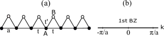
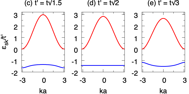
Figure 1: Sawtooth lattice is a linear-chain model with a two-point basis (a), and its first Brillouin zone lies on a straight line (b). Typical band structures (c-e) feature a flat band with energy $\varepsilon_{-,k}=-2t$ when $t^{\prime}=t\sqrt{2}$.

In this paper we allow hopping processes between nearest-neighbor sites only, and set $t_{Aj;Ai}^{\sigma}=-t$ with $j=i\pm 1$ and $t\geq 0$, $t_{Bj;Bi}^{\sigma}=0$ and $t_{Bi;Ai}^{\sigma}=t_{Bj;Ai}^{\sigma}=-t^{\prime}$ with $j=i-1$ and $t^{\prime}\geq 0$. It is called the zigzag model when $t_{Bj;Bi}^{\sigma}\neq t^{\prime\prime}$ for $j=i\pm 1$. Then the single-particle Hamiltonian can be written as

$$H_{\sigma}=\sum_{k}\begin{pmatrix}c_{Ak\sigma}^{\dagger}&c_{Bk\sigma}^{\dagger}\end{pmatrix}\begin{pmatrix}d_{k}^{0}+d_{k}^{z}&d_{k}^{x}-id_{k}^{y}\\ d_{k}^{x}+id_{k}^{y}&d_{k}^{0}-d_{k}^{z}\\ \end{pmatrix}\begin{pmatrix}c_{Ak\sigma}\\ c_{Bk\sigma}\end{pmatrix},$$ (22)

where the wave vector $k\in\textrm{BZ}$, and the matrix elements are $d_{k}^{0}=d_{k}^{z}=t\cos(ka),$ $d_{k}^{x}=t^{\prime}+t^{\prime}\cos(ka)$ and $d_{k}^{y}=t^{\prime}\sin(ka).$ Thus the single-particle energy bands disperse as $\varepsilon_{sk\sigma}=d_{k}^{0}+sd_{k}$ where $s=\pm$ labels the upper and lower bands, respectively, and $d_{k}=\sqrt{(d_{k}^{x})^{2}+(d_{k}^{y})^{2}+(d_{k}^{z})^{2}}.$ The corresponding eigenvectors are determined by $s_{Ak\sigma}=\langle A|sk\sigma\rangle=\frac{-d_{k}^{x}+id_{k}^{y}}{\sqrt{2d_{k}(d_{k}-sd_{k}^{z})}}$ and $s_{Bk\sigma}=\langle B|sk\sigma\rangle=\frac{d_{k}^{z}-sd_{k}}{\sqrt{2d_{k}(d_{k}-sd_{k}^{z})}}.$ We illustrate typical band structures $\varepsilon_{sk}=\varepsilon_{sk\sigma}$ in Figs. 1(c), 1(d) and 1(e). It is shown that while the lower band is flat with energy $\varepsilon_{-,k}=-2t$ when $t^{\prime}/t=\sqrt{2}$, it has a positive (negative) curvature when $t^{\prime}/t$ is greater (lesser) than $\sqrt{2}$.

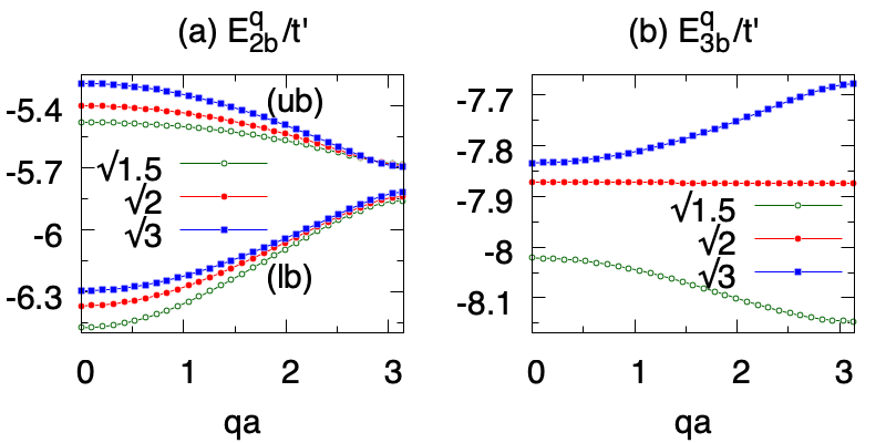
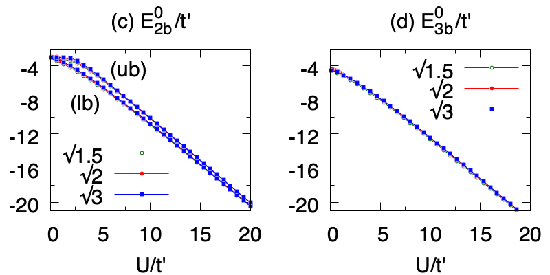
Figure 2: (a) There are two distinct two-body bound states $E_{2b}^{q}$ for a given total momentum $q$ of the two particles: upper branch (ub) and lower one (lb). The lower branch plays an important role in the stability of the trimers [see the discussion around Eq. (23)]. (b) The energy of the lowest three-body bound state $E_{3b}^{q}$ as a function of total momentum $q$ of the three particles. While $E_{3b}^{q}$ of the flat-band case has a small dispersion that is similar in shape to that of the $\sqrt{1.5}$ case, it appears quite flat in the shown scale. (c-d) $E_{2b}^{0}$ and $E_{3b}^{0}$ as a function of interaction. In all figures green-hollow-circles, red-filled-circles and blue-filled-squares correspond, respectively, to $t^{\prime}/t=\{\sqrt{1.5},\sqrt{2},\sqrt{3}\}$ that are illustrated in Figs. 1(c), 1(d) and 1(e). They are on top of each other in (c) and (d) except for the weak-coupling limit. In addition we set $U=5t^{\prime}$ in (a) and (b).

In Figs. 2(a) and 2(b), we set $U=5t^{\prime}$, and present, respectively, the corresponding solutions for the two-body ($E_{2b}^{q}$) and the three-body ($E_{3b}^{q}$) bound states as a function of $q$. Here $q$ stands, respectively, for the total momentum of two and three particles involved. Since $N_{b}=2$, there are two distinct $E_{2b}^{q}$ solutions for a given $q$: upper branch (ub) and lower one (lb). The lower branch plays an important role in the stability of the trimers as discussed below. We find that the $q$-dependences of $E_{2b}^{q}$ are qualitatively similar to each other for all three hoppings considered in Figs. 1(c), 1(d) and 1(e). In contrast, the $q$-dependences of $E_{3b}^{q}$ are quite distinct: while it has a positive (negative) curvature near the origin (edge) of the BZ when $t^{\prime}/t=\sqrt{3}$, it has a negative (positive) curvature near the origin (edge) of the BZ when $t^{\prime}/t=\sqrt{1.5}$. We also find that $E_{3b}^{q}$ of the flat-band case has a small dispersion that is similar in shape to that of the $\sqrt{1.5}$ case, but it appears quite flat in the shown scale. Its bandwidth $\sim 0.001204t^{\prime}$ starts from $-7.872373t^{\prime}$ at $q=0$ and decreases to $-7.873577t^{\prime}$ at $q=\pi/a$. In the low-$qa$ limit we find the following fitting functions for Fig. 2(b): $E_{3b}^{q}/t^{\prime}\approx-8.021633-0.0235a^{2}q^{2}$ in the range $qa\lesssim 1$ when $t^{\prime}/t=\sqrt{1.5}$, $E_{3b}^{q}/t^{\prime}\approx-7.872373-0.000635a^{2}q^{2}$ in the range $qa\lesssim 0.5$ when $t^{\prime}/t=\sqrt{2}$, and $E_{3b}^{q}/t^{\prime}\approx-7.833807+0.0221a^{2}q^{2}$ in the range $qa\lesssim 1$ when $t^{\prime}/t=\sqrt{3}$. All of these results are obtained with $N_{c}=100$ mesh points in the BZ, and we checked that increasing it to $N_{c}=200$ makes minor changes. Thus the flatness of the $E_{3b}^{q}$ when $t^{\prime}/t=\sqrt{2}$ is partly caused by the large effective-mass of the three-body bound states. In Figs. 2(c) and 2(d), we set $q=0$, and present, respectively, $E_{2b}^{0}$ and $E_{3b}^{0}$ as a function of $U$. They appear on top of each other for different values of $t$ except for the weak-coupling limit.

In order to be observed, a three-body bound state (trimer) must be energetically stable against two distinct dissociation mechanisms shi14 : (i) free-atom dissociation threshold where the trimer decays into two free spin-$\uparrow$ particles and a free spin-$\downarrow$ particle, and (ii) atom-dimer dissociation threshold where the trimer decays into a two-body bound state (dimer) and a free spin-$\uparrow$ particle. Since the former mechanism requires higher-energy processes in the parameter regime of interest in our numerical calculations, it is the second mechanism that determines the binding energy $E_{\textrm{trimer}}^{\mathbf{q}}$ of the trimers. For this reason we define $E_{\textrm{trimer}}^{\mathbf{q}}$ with respect to the atom-dimer dissociation threshold as

$$E_{\textrm{trimer}}^{\mathbf{q}}=-E_{3b}^{\mathbf{q}}+\min\{E_{2b}^{\mathbf{q^{\prime}}}+\varepsilon_{n,\mathbf{q}-\mathbf{q^{\prime}},\uparrow}\}.$$ (23)

In Fig. 3(a) we set $U=5t^{\prime}$, and present the resultant $E_{\textrm{trimer}}^{q}$ as a function of $q$ for the corresponding data shown in Figs. 2(a) and 2(b). We found very similar results for most of the parameter regimes of interest here, e.g., $U=10t^{\prime}$ is shown in Fig. 3(b). In particular, in the flat-band case when $t^{\prime}/t=\sqrt{2}$, the atom-dimer dissociation threshold is given by $\min\{E_{2b}^{q^{\prime}}+\varepsilon_{n,q-q^{\prime},\uparrow}\}=\min\{E_{2b}^{q^{\prime}}\}-2t=E_{2b}^{0}-2t.$ This is because the dimer ground-state is at $q=0$, and $E_{2b}^{0}$ is the minimum of the lower branch in the two-body problem. Thus while $E_{\textrm{trimer}}^{q}$ of the flatband case has a small dispersion with a positive (upward) curvature coming from $-E_{3b}^{\mathbf{q}}$, it appears quite flat in the shown scale. To illustrate its dispersive nature we present $E_{\textrm{trimer}}^{q}-E_{\textrm{trimer}}^{0}$ in Fig. 3(c) for $U/t^{\prime}=\{2,5,10\},$ where $E_{\textrm{trimer}}^{0}/t^{\prime}\sim\{0.023,0.091,0.20\},$ respectively. This figure suggests that $E_{\textrm{trimer}}^{q}$ may have a sizeable dispersion only in the weak-coupling limit when $E_{\textrm{trimer}}^{0}$ is small. Unfortunately our numerical accuracy becomes unreliable in this limit, and we could not fully resolve this point. This is because as the size of the trimers (in real space) is expected to increase dramatically in the $E_{\textrm{trimer}}^{0}/t^{\prime}\to 0$ limit, their precise calculation requires a much larger lattice size, i.e., one must choose larger and larger number of unit cells $N_{c}\to\infty$ as $U/t^{\prime}\to 0$.

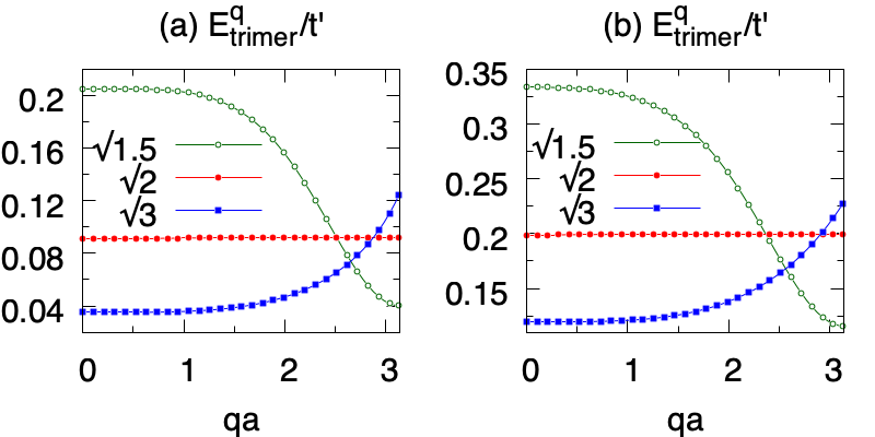
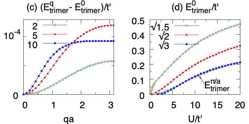
Figure 3: (a - b) Binding energy of the three-body bound state $E_{\textrm{trimer}}^{q}$ as a function of total momentum $q$ of the three particles when $U=5t^{\prime}$ and $U=10t^{\prime}$, respectively. While $E_{\textrm{trimer}}^{q}$ of the flat-band case has a small dispersion with a positive (upward) curvature near the origin, it appears quite flat in the shown scale. This is illustrated in (c) where $E_{\textrm{trimer}}^{q}-E_{\textrm{trimer}}^{0}$ is shown as a function of $q$ for $U/t^{\prime}=\{2,5,10\}$ when $t^{\prime}=t\sqrt{2}$. (d) $E_{\textrm{trimer}}^{0}$ as a function of interaction. $E_{\textrm{trimer}}^{\pi/a}$ is also shown for $t^{\prime}=t\sqrt{1.5}$ but it is barely visible since it overlaps with the $E_{\textrm{trimer}}^{0}$ of $t^{\prime}=t\sqrt{3}$ in most parts. Note that $E_{\textrm{trimer}}^{0}$ of the flat-band case is consistent with the very recent DMRG results (see their Fig. 10) orso21 . In (a), (b) and (d) the green-hollow-circles, red-filled-circles and blue-filled-squares correspond, respectively, to $t^{\prime}/t=\{\sqrt{1.5},\sqrt{2},\sqrt{3}\}$ that are illustrated in Figs. 1 and 2.

Furthermore Figs. 3(a) and 3(b) shows that while the binding-energy of the ground-state trimer is at $q=\pi/a$ when $t^{\prime}/t=\sqrt{1.5}$, it is at $q=0$ when $t^{\prime}/t=\sqrt{2}$ or $\sqrt{3}$. The origin of this difference can be traced back to the location of the single-particle ground state, i.e., see the corresponding band structures in Figs. 1(c), 1(d) and 1(e), respectively. In order to reveal the fate of trimer states as a function of $U$, we set $q=0$, and present the resultant $E_{\textrm{trimer}}^{0}$ in Fig. 3(d) for the corresponding data shown in Figs. 2(c) and 2(d). We also show $E_{\textrm{trimer}}^{\pi/a}$ for the $t^{\prime}=t\sqrt{1.5}$ case but it is barely visible since it overlaps with the $E_{\textrm{trimer}}^{0}$ of $t^{\prime}=t\sqrt{3}$ in most parts. In addition $E_{\textrm{trimer}}^{0}$ of the $t^{\prime}=t\sqrt{1.5}$ case is shown for completeness. First of all it is delightful to note that $E_{\textrm{trimer}}^{0}$ of the flat-band case seems to be in very good agreement with the recent DMRG results, i.e., compare it with Fig. 10 of orso21 . In this case our numerical findings suggest that there exist trimer states that are energetically stable for all interaction strengths including the weak-coupling limit no matter how small $U/t^{\prime}$ is.

On the other hand, when $t^{\prime}/t$ deviates from $\sqrt{2}$, there seems to be a finite threshold in the $U/t^{\prime}\to 0$ limit. For instance $E_{\textrm{trimer}}^{0}$ of the $t^{\prime}/t=\sqrt{3}$ case is shown in Fig. 3(d), and we also verified it to be the case for the $t^{\prime}/t=\sqrt{6}$ case but it is not presented. In addition $E_{\textrm{trimer}}^{\pi/a}$ of the $t^{\prime}/t=\sqrt{1.5}$ case is again shown in Fig. 3(d), and we also verified it to be the case for the $t^{\prime}/t=1$ case but is again not presented. It is numerically challenging to pinpoint the exact location of the interaction thresholds in the $U/t^{\prime}\to 0$ limit since the binding energy of the ground-state trimers, i.e., $E_{\textrm{trimer}}^{0}$ or $E_{\textrm{trimer}}^{\pi/a}$, gradually approaches to zero with a long tail. However we observe that the thresholds tend to increase further and further as a function of increasing deviation from the flat-band limit $t^{\prime}/t=\sqrt{2}$, i.e., the threshold for the $t^{\prime}/t=1$ case is considerably higher than that of $t^{\prime}/t=\sqrt{1.5}$ and the threshold for the $t^{\prime}/t=\sqrt{6}$ case is considerably higher than that of $t^{\prime}/t=\sqrt{3}$. Our naive expectation is that the sawtooth model must recover the linear-chain model in either (i) the $t^{\prime}/t\gg 1$ or (ii) the $t^{\prime}/t\ll 1$ limit. In fact, in agreement with our numerical results, stable trimers are known not to be allowed in a single-band linear-chain model mattis86 ; orso10 ; orso11 . Thus our results establish that the formation of stable trimers is a genuine multiband effect mediated by the interband transitions.

V Conclusion

To summarize here we solved the three-body problem in a generic multiband Hubbard model, and reduced it to an eigenvalue problem for the dispersion of the trimer states. As an illustration we applied our theory to the sawtooth lattice with a two-point basis, and showed that the trimer states are allowed in a broad range of model parameters. This finding is in sharp contrast with the single-band linear-chain model mattis86 ; orso10 ; orso11 and it is in very good agreement with the recent DMRG results orso21 . In addition we found that the trimers have a nearly-flat dispersion with a negligible bandwidth when formed in a flat band, which is unlike the highly-dispersive spectrum of its dimers. As an outlook our generic results may find direct applications in higher-dimensional lattices with more complicated lattice geometries and band structures mizoguchi19 . For instance the fate of trimers in a Kagome lattice could be an interesting problem iskin22 . Such an analysis would reveal not only the impact of higher bands on the trimer states but also the role played by the lattice dimensionality. Furthermore it is a straightforward task to extend our approach and analyze the nature of trimer states with three identical bosons in the presence of multiple Bloch bands mattis86 ; valiente10 .

As a final remark we have recently generalized our approach to the ($N+1$)-body problem in a generic multiband lattice, and derived the integral equations for the bound states of $N$ spin-$\uparrow$ fermions and a spin-$\downarrow$ fermion due to an onsite attraction in between iskin22 . Our numerical calculations for the $N=3$ case shows that the tetramer states are also allowed in the sawtooth lattice, e.g., they also have a nearly-flat dispersion with a negligible bandwidth when formed in a flat band. It turns out larger cluster states, i.e., pentamers and beyond, are also possible in this system but, unfortunately, one may have to resort to a high-performance computer to solve the resultant matrices when $N\geq 4$. They are numerically very expensive and well beyond our current capacity.

References

(1)
H. Tasaki,
The Hubbard model - an introduction and selected rigorous results,
J. Phys.: Condens. Matter 10, 4353 (1998).
(2)
D. P. Arovas, E. Berg, S. Kivelson, and S. Raghu,
The Hubbard Model,
Annu. Rev. Condens. Matter Phys., 10.1146/annurev-conmatphys-031620-102024 (2021)
(3)
M. Qin, T. Schäfer, S. Andergassen, P. Corboz, and E. Gull,
The Hubbard Model: A Computational Perspective,
Annu. Rev. Condens. Matter Phys., 10.1146/annurev-conmatphys-090921-033948 (2021).
(4)
C. Gross and I. Bloch,
Quantum simulations with ultracold atoms in optical lattices,
Science 357, 995 (2017).
(5)
T. Esslinger,
Fermi-Hubbard physics with atoms in an optical lattice,
Annu. Rev. Condens. Matter Phys., 10.1146/annurev-conmatphys-070909-104059 (2010).
(6)
T. Kraemer, M. Mark, P. Waldburger, J. G. Danzl, C. Chin, B. Engeser, A. D. Lange, K. Pilch,
A. Jaakkola, H.-C. Nägerl, and R. Grimm,
Evidence for Efimov quantum states in an ultracold gas of caesium atoms.
Nature 440, 315 (2006).
(7)
M. Zaccanti, B. Deissler, C. D’Errico, M. Fattori, M. Jona-Lasinio, S. Müller,
G. Roati, M. Inguscio, and G. Modugno,
Observation of an Efimov spectrum in an atomic system,
Nature Phys. 5, 586 (2009).
(8)
S. E. Pollack, D. Dries, and R. G. Hulet,
Universality in Three- and Four-Body Bound States of Ultracold Atoms,
Science 326, 1683 (2009).
(9)
E. Braaten and H.-W. Hammer,
Universality in few-body systems with large scattering length,
Phys. Rept. 428, 259 (2006).
(10)
C. H. Greene, P. Giannakeas, and J. Pérez-Ríos,
Universal few-body physics and cluster formation
Rev. Mod. Phys. 89, 035006 (2017).
(11)
P. Naidon and S. Endo,
Efimov physics: A review,
Rep. Prog. Phys. 80, 056001 (2017).
(12)
N. T. Zinner,
Few-body physics in a many-body world,
Few-Body Systems 55, 599 (2014).
(13)
O. I. Kartavtsev and A. V. Malykh,
Low-energy three-body dynamics in binary quantum gases,
J. Phys. B: 40, 1429 (2007).
(14)
Z.-Y. Shi, X. Cui, and H. Zhai,
Universal Trimers Induced by Spin-Orbit Coupling in Ultracold Fermi Gases,
Phys. Rev. Lett. 112, 013201 (2014).
(15)
X. Cui and W. Yi,
Universal Borromean Binding in Spin-Orbit-Coupled Ultracold Fermi Gases,
Phys. Rev. X 4, 031026 (2014).
(16)
Q. Ji, R. Zhang, and W. Zhang,
Universal and Efimov trimers in an alkaline-earth-metal and alkali-metal gas mixture with spin-orbit coupling,
Phys. Rev. A 102, 063313 (2020).
(17)
G.-B. Jo, J. Guzman, C. K. Thomas, P. Hosur, A. Vishwanath, and D. M. Stamper-Kurn,
Ultracold Atoms in a Tunable Optical Kagome Lattice,
Phys. Rev. Lett. 108, 045305 (2012).
(18)
Y. Nakata, T. Okada, T. Nakanishi, and M. Kitano,
Observation of flat band for terahertz spoof plasmons in a metallic Kagomé lattice,
Phys. Rev. B 85, 205128 (2012).
(19)
Z. Li, J. Zhuang, L. Wang, H. Feng, Q. Gao, X. Xu, W. Hao, X. Wang, C. Zhang,
K. Wu, S. X. Dou, L. Chen, Z. Hu, and Y. Du,
Realization of flat band with possible nontrivial topology in electronic Kagome lattice,
Science Advances 4, eaau4511 (2018).
(20)
F. Diebel, D. Leykam, S. Kroesen, C. Denz, and A. S. Desyatnikov
Conical Diffraction and Composite Lieb Bosons in Photonic Lattices,
Phys. Rev. Lett. 116, 183902 (2016).
(21)
S. Kajiwara, Y. Urade, Y. Nakata, T. Nakanishi, and M. Kitano,
Observation of a nonradiative flat band for spoof surface plasmons in a metallic Lieb lattice,
Phys. Rev. B 93, 075126 (2016).
(22)
H. Ozawa, S. Taie, T. Ichinose, and Y. Takahashi,
Interaction-Driven Shift and Distortion of a Flat Band in an Optical Lieb Lattice,
Phys. Rev. Lett. 118, 175301 (2017).
(23)
H. Tasaki,
From Nagaoka’s Ferromagnetism to Flat-Band Ferromagnetism and Beyond:
An Introduction to Ferromagnetism in the Hubbard Model,
Prog. of Theoretical Physics 99, 489 (1998).
(24)
S. A. Parameswaran, R. Roy, and S. L. Sondhi,
Fractional Quantum Hall Physics in Topological Flat Bands,
Comptes Rendus Physique 14, 816 (2013).
(25)
Z. Liu, F. Liu, and Yong-Shi Wu,
Exotic electronic states in the world of flat bands: from theory to material,
Chin. Phys. B 23, 077308 (2014).
(26)
D. Leykam, A. Andreanov, and S. Flach,
Artificial flat band systems: from lattice models to experiments,
Adv. Phys.: X 3, 1473052 (2018).
(27)
L. Balents, C. R. Dean, D. K. Efetov, and A. F. Young,
Superconductivity and strong correlations in moiré flat bands,
Nat. Phys. 16, 725 (2020).
(28)
G. Orso and M. Singh,
Formation of bound states and BCS-BEC crossover near a flat band: the sawtooth lattice,
arXiv:2112.10188.
(29)
M. Iskin,
Two-body problem in a multiband lattice and the role of quantum geometry,
Phys. Rev. A 103, 053311 (2021).
(30)
D. C. Mattis,
The few-body problem on a lattice,
Rev. Mod. Phys. 58, 361 (1986).
(31)
G. Orso, E. Burovski, and T. Jolicoeur,
Luttinger Liquid of Trimers in Fermi Gases with Unequal Masses,
Phys. Rev. Lett. 104, 065301 (2010).
(32)
G. Orso, E. Burovski, and T. Jolicoeur,
Fermionic trimers in spin-dependent optical lattices,
CRAS (Paris) Physique 12, 39 (2011).
(33)
M. Iskin,
Effective-mass tensor of the two-body bound states and the quantum-metric tensor of
the underlying Bloch states in multiband lattices,
Phys. Rev. A 105, 023312 (2022).
(34)
T. Zhang and G.-B. Jo,
One-dimensional sawtooth and zigzag lattices for ultracold atoms,
Sci. Rep. 5, 16044 (2015).
(35)
V. A. J. Pyykkönen, S. Peotta, P. Fabritius, J. Mohan, T. Esslinger, and P. Törmä,
Flat-band transport and Josephson effect through a finite-size sawtooth lattice,
Phys. Rev. B 103, 144519 (2021).
(36)
S. M. Chan, B. Grémaud, and G. G. Batrouni,
Pairing and superconductivity in quasi one-dimensional flat band systems:
Creutz and sawtooth lattices,
Phys. Rev. B 105, 024502 (2022).
(37)
T. Mizoguchi and M. Udagawa,
Flat-band engineering in tight-binding models: Beyond the nearest-neighbor hopping,
Phys. Rev. B 99, 235118 (2019).
(38)
M. Valiente, D. Petrosyan, and A. Saenz,
Three-body bound states in a lattice,
Phys. Rev. A 81, 011601(R) (2010).
(39) M. Iskin and A. Keleş,
Few-body clusters in a multiband Hubbard model: Tetramers, pentamers, and beyond,
arXiv:2204.10003 (2022).