Machine-assisted discovery of integrable symplectic mappings

Abstract

We present a new automated method for finding integrable symplectic maps of the plane. These dynamical systems possess a hidden symmetry associated with an existence of conserved quantities, i.e. integrals of motion. The core idea of the algorithm is based on the knowledge that the evolution of an integrable system in the phase space is restricted to a lower-dimensional submanifold. Limiting ourselves to polygon invariants of motion, we analyze the shape of individual trajectories thus successfully distinguishing integrable motion from chaotic cases. For example, our method rediscovers some of the famous McMillan-Suris integrable mappings and ultra-discrete Painlevé equations. In total, over 100 new integrable families are presented and analyzed; some of them are isolated in the space of parameters, and some of them are families with one parameter (or the ratio of parameters) being continuous or discrete. At the end of the paper, we suggest how newly discovered maps are related to a general 2D symplectic map via an introduction of discrete perturbation theory and propose a method on how to construct smooth near-integrable dynamical systems based on mappings with polygon invariants.

I Introduction

Integrable systems play a fundamental role in mathematics and physics, particularly in dynamical system theory, due to well-understood dynamics. Integrability is generally defined as the existence of a sufficient number of functionally independent conserved quantities (integrals of motion) in involution, which are related to intricate hidden symmetries. Hence, in many cases the construction of integrable systems often requires some special fine-tuning. This makes them very difficult to discover. Although integrable models occupy measure-zero in the space of parameters, they play a crucial role in the theory of dynamical systems. In fact, they shed light on the properties of more generic near-integrable cases via Kolmogorov-Arnold-Moser (KAM) theorem and various perturbation theories.

While the concept of integrability is most often discussed in the context of continuous-time systems, it also arises in discrete-time maps Arnold and Avez (1968). Mappings are of profound importance in the field of dynamical system theory exhibiting a broad range of behaviours including dynamical chaos, bifurcations, strange attractors, and integrability Lichtenberg and Lieberman (2013). On the one hand, they can be used as an approximation of a continuous flow (since in many cases the discretized form can be easier to study) or as a reduction to a lower dimensional manifold, e.g., considering Poincaré cross-sections. A particularly valuable class of discrete dynamical systems are symplectic maps, associated with Hamiltonian flows, e.g., a 2D area-preserving map is equivalent to a Hamiltonian system with 1 degree of freedom and a potential energy that is periodic in time. Symplectic maps arise as effective models in a wide range of domains, such as celestial mechanics, plasma hydrodynamics, fluid flows, and particle accelerators Meiss (1992).

Although area-preserving maps of the plane have been studied for decades, only a handful of integrable cases have been discovered. The existence of integrals of motion restricts phase space dynamics to a set of nested tori. Any discovery of novel integrable maps is highly non-trivial and historically has been accomplished by scientists making inspired guesses and applying relevant analytical tools. In many cases, even the proof of the integrability of a specific mapping is quite challenging.

An automated search for integrable systems remains a nontrivial task: only a few successful examples exist to date where machine-assisted searches resulted in new discoveries in nonlinear dynamics. For example, computer-assisted searches combined with high precision simulations found new families of periodic orbits in a gravitational three-body problem Šuvakov and Dmitrašinović (2013); Li and Liao (2017); Li et al. (2018). Recent works utilized machine-learning methods to discover integrals of motion of classical dynamical systems from phase space trajectories, e.g. Refs. Bondesan and Lamacraft (2019); Liu and Tegmark (2021); Ha and Jeong (2021); Wetzel et al. (2020). These examples employed a computer-assisted search to either discover new families of trajectories or to rediscover previously known invariants of motion in integrable systems. In contrast, our algorithm has found previously unknown integrable symplectic maps, advancing the theory of integrable systems.

In this paper, we propose and describe this new algorithm for discovering area-preserving integrable maps of the plane. While scanning over a large space of potential candidate maps, our algorithm traces out individual orbits and subsequently analyzes shapes of invariant manifolds. We restricted our search to the family of mappings which possess integrals of motion with a polygon geometry, thus constraining our search to piecewise linear transformations of the plane. Piecewise linear mappings could be regarded as the simplest possible dynamical systems with rich nonlinear dynamics, which makes them an attractive model to study. They could be viewed as fundamental building blocks of generic integrable symplectic maps. An arbitrary smooth 2D symplectic map could be approximated as an $n$-piece piecewise linear map, but only in the uniform sense, see Section VIII.3. By applying a machine-assisted search, we found over a hundred new integrable mappings; some of them are isolated in the space of parameters, and some of them are families with one parameter (or the ratio of parameters) being continuous ($\in\mathbb{R}^{(+)}$) or discrete ($\in\mathbb{Z}^{(+)}$).

The structure of this article is as follows. In Section II we provide a historical overview of integrability of symplectic mappings of the plane. In Sections III and IV we review linear integrable mappings produced by 1- and 2-piecewise linear force functions. At the end of Section IV we introduce nonlinear integrable mappings with polygon invariants, and in Section V we propose an algorithm for the machine-assisted discovery of integrable systems with more complicated force functions. Sections VI and VII presents the main results of our search, and finally, in Section VIII we discuss some practical applications of mappings with polygon invariants. Several appendices contain supplementary materials, tables with dynamical properties of mappings, and a pseudo-code for the search algorithm.

II 2D symplectic mappings and integrability: historical overview

The most general form of an autonomous 2D mapping of the plane, $\mathcal{M}:\mathbb{R}^{2}\to\mathbb{R}^{2}$, can be written as

$$\begin{array}[]{l}q^{\prime}=F(q,p),\\[5.69046pt] p^{\prime}=G(q,p),\end{array}$$

where ^′ denotes an application of the map, and $F$ and $G$ are functions of both variables. If the Jacobian of a 2D map, $J\equiv\partial_{q}F\,\partial_{p}G-\partial_{p}F\,\partial_{q}G$, is equal to unity, then the map is area-preserving and thus also symplectic (for higher dimensional mappings, the volume-preservation is necessary but not sufficient for a map to be symplectic). A map is called integrable in a Liouville sense Veselov (1991) if there exists a real-valued continuous function $\mathcal{K}(p,q)$ called an integral of motion (or invariant), for which the level sets $\mathcal{K}(p,q)=\mathrm{const}$ are curves (or sets of points) and

$$\forall\,(q,p)\in\mathbb{R}^{2}:\qquad\mathcal{K}(p^{\prime},q^{\prime})=\mathcal{K}(p,q).$$

The first nonlinear symplectic integrable map of the plane was discovered by E. McMillan McMillan (1971) when he studied a very specific form of the map

$$\begin{array}[]{l}q^{\prime}=p,\\[5.69046pt] p^{\prime}=-q+f(p),\end{array}$$ (1)

where $f(p)$ will be called the force function. We will refer to this mapping as the McMillan-Hénon form or the MH form for short (please do not confuse with McMillan integrable map McMillan (1971), which is a special case when $f(p)$ is given by a ratio of two quadratic polynomials).

At first, the choice of the MH form (1) might look very restrictive and unmotivated. McMillan’s original idea was based on its simplicity and clear symmetries (which will be described in detail below), which still allowed some degree of freedom in modifying the dynamics by varying $f(p)$. As it was demonstrated later by D. Turaev Turaev (2002), almost every symplectic map of the plane (and even 2$n$D symplectic map) can be approximated by iterations of MH maps. In this article, we will restrict our consideration to this form; however, our results can be easily generalized to different representations of the map.

Below we summarize several important results regarding the integrability of mappings in a McMillan-Hénon form:

1. First, the family of integrable mappings of the plane in the MH form were discovered by McMillan McMillan (1971) for a biquadratic invariant in the form

   $$(\mathrm{I}):\qquad\mathcal{K}(p,q)=\mathrm{A}\,p^{2}q^{2}+\mathrm{B}\,(p^{2}q+p\,q^{2})+\Gamma\,(p^{2}+q^{2})+\Delta\,p\,q+\mathrm{E}\,(p+q)$$

   corresponding to the force function

   $$f(p)=\frac{\mathrm{B}\,p^{2}+\Delta\,p+\mathrm{E}}{\mathrm{A}\,p^{2}+\mathrm{B}\,p+\Gamma}$$

   and integrable for any values of parameters $\mathrm{A}$, $\mathrm{B}$, $\Gamma$, $\Delta$ and $\mathrm{E}$ (Fig. 1a).

2. Later, Y. Suris Suris (1989) studied the integrability of a difference equation in the form $x_{n+1}+x_{n-1}=f(x_{n})$ referred to as the Suris form of the map (sometimes referred to as the standard type). The Suris form of the mapping has a clear physical interpretation, since in the continuous-time limit it takes a form of a 1D Newton equation $\ddot{x}=f(x)-2\,x$, where the right hand side plays a role of a mechanical force. Mapping in the Suris form is just another representation of the MH form by setting $q_{n}=x_{n}$ and $p_{n}=x_{n+1}$ (one can think of an analogy between the Lagrangian approach with a single differential equation of the second order, and the Hamiltonian approach with two differential equations of the first order, e.g. see Veselov (1991)). Suris proved that for analytic force functions $f(p)$ and $\mathcal{K}(p,q)$, the invariant of the integrable mapping can take only one of the forms: (I) biquadratic function of $p$ and $q$ (McMillan map), (II) biquadratic exponential or (III) trigonometric polynomial:

   $$\begin{array}[]{ll}(\mathrm{II}):&\displaystyle\mathcal{K}(p,q)=\mathrm{A}\,e^{\alpha\,p}e^{\alpha\,q}+\mathrm{B}\,(e^{\alpha\,p}+e^{\alpha\,q})+\Gamma\,(e^{\alpha\,p}e^{-\alpha\,q}+e^{-\alpha\,p}e^{\alpha\,q})+\Delta\,(e^{-\alpha\,p}+e^{-\alpha\,q})+\mathrm{E}\,e^{-\alpha\,p}e^{-\alpha\,q},\\[7.11317pt] (\mathrm{III}):&\displaystyle\mathcal{K}(p,q)=\Lambda_{1}\,(\cos[\omega\,p-\psi]+\cos[\omega\,q-\psi])+\Lambda_{2}\,\cos[\omega\,(p+q)-\phi]+\Lambda_{3}\,\cos[\omega\,(p-q)],\\[7.11317pt] \mathrm{and}&\displaystyle f_{\mathrm{II}}(q)=\frac{1}{\alpha}\,\log\left[\frac{\Gamma\,e^{\alpha\,q}+\Delta+\mathrm{E}\,e^{-\alpha\,q}}{\mathrm{A}\,e^{\alpha\,q}+\mathrm{B}+\Gamma\,e^{-\alpha\,q}}\right],\qquad f_{\mathrm{III}}(q)=\frac{2}{\omega}\,\arctan\left[\frac{\Lambda_{1}\sin\Phi+\Lambda_{2}\sin(\Psi-q)+\Lambda_{3}\sin q}{\Lambda_{1}\cos\Phi+\Lambda_{2}\cos(\Psi-q)+\Lambda_{3}\cos q}\right].\end{array}$$

   Mappings (I – III) are integrable for any choice of parameters, see some examples with invariant level sets in Fig. 1 (a. – c.). Results by Suris greatly reduce possible forms of $f(p)$ corresponding to integrable maps.

   

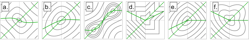
   Figure 1: Invariant level sets, $\mathcal{K}(p,q)=\mathrm{const}$, for integrable mappings in the MH form. McMillan-Suris mappings I – III, respectively (a.) – (c.), with $\mathrm{A},\Gamma,\Delta,\Lambda_{1,3}=-\Lambda_{2}=1$ and $\mathrm{B},\mathrm{E},\psi,\phi=0$. Brown-Knuth map (d.) along with McMillan beheaded (e.) and two-headed (f.) ellipses. All mappings are shown for the range $q,p\in[-2,2]$. The dashed and solid dark green lines show the first and second symmetry lines.

3. In 1983 Morton Brown proposed an interesting problem in the section “Advanced Problems” of Amer. Math. Monthly Brown (1983).

   6439. Let $\{x_{n}\}$ be a sequence of real numbers satisfying the relation $x_{n+1}=|x_{n}|-x_{n-1}$. Prove that $\{x_{n}\}$ is periodic with period 9.

   One can notice that this map is in the Suris form (so it can be written in the MH form as well) with $f(p)=|p|$.

   In 1985 the solution by J. F. Slifker was published in Brown and Slifker (1985) with a comment below:

   Also solved by the proposer and sixty-one others. The problem turned out to be rather elementary.

   Despite its “simplicity,” the map has proven to be interesting for dynamical system theory, combinatorics and topology. 10 years later, in 1993, Brown extended his results to the formal publication Brown (1993). He reconsidered the equation as the homeomorphism of the plane and provided a geometrical proof of periodicity including a description of the polygon invariant of motion (see Fig. 1d):

   $$\mathcal{K}(p,q)=q+\big{|}q-|p|\big{|}+\Big{|}p-\big{|}q-|p|\big{|}\Big{|}+\Big{|}q-\big{|}p-|q|\big{|}\Big{|}+\bigg{|}p-|q|+\Big{|}q-\big{|}p-|q|\big{|}\Big{|}\bigg{|}.$$

   D. Knuth, who provided his own combinatorical proof of periodicity, wrote a letter to Brown:

   When I saw advanced problem 6439, I couldn’t believe that it was “advanced”: a result like that has to be either false or elementary!

   But I soon found that it wasn’t trivial. There is a simple proof, yet I can’t figure out how on earth anybody would discover such a remarkable result. Nor have I discovered any similar recurrence relations having the same property. So in a sense I have no idea how to solve the problem properly. Is there an “insightful” proof, or is the result simply true by chance?

   While quite often this map is referred to as Knuth map, we would like to call it Brown-Knuth map to acknowledge all contributors.

4. Finally, in his original article McMillan (1971), Edwin McMillan suggested another intricate integrable system with a piecewise quadratic invariant and a piecewise linear force function

   $$\mathcal{K}(p,q)=\left\{\begin{array}[]{l}p^{2}+a\,p\,q+q^{2},\qquad p,q\geq 0,\\[5.69046pt] p^{2}-a\,p\,q+q^{2},\qquad\mathrm{otherwise},\end{array}\right.\qquad\mathrm{and}\qquad f(p)=\left\{\begin{array}[]{ll}a\,p,&q<0,\\[5.69046pt] 0,&q\geq 0,\end{array}\right.$$

   where $a\in\mathbb{R}$ is an arbitrary coefficient. He referred to the corresponding invariant level sets as beheaded and two-headed ellipses (Fig. 1e). As we will see in Section IV.1.2, this map as well as Brown-Knuth map are examples of more general integrable systems with the force function $f(p)=a\,p+b\,|p|$ and invariants being collection of ellipses, hyperbolas and straight lines (segments).

5. At the end, we should mention a special class of finite difference equations, which are integrable (in the sense that they admit a Lax pair representation), known as discrete Painlevé equations. Discrete Painlevé equations are closely related to integrable symplectic maps of the plane. We discuss the connection in Section VIII.1.

Several properties of MH mappings (1) which will help us to understand and interpret further results are:

• A map in the MH form is symplectic and reversible for any continuous $f(p)$, with the inverse

  $$\begin{array}[]{ll}\mathcal{M}^{-1}:\quad\begin{cases}q^{\prime}=-p+f(q),\\ p^{\prime}=q.\end{cases}\end{array}$$

• For any map with $f(p)$ there is a twin map with the mirrored force function $-f(-p)$, so that their dynamics are identical up to a rotation of phase space by an angle of $\pi$, $(p,q)\rightarrow-(p,q)$. Thus, we will omit twin maps unless it is necessary.

• A MH map can be decomposed into two transformations $\mathcal{M}=\mathcal{F}\circ\mathrm{Rot}(\pi/2)$, where

  $$\begin{array}[]{ll}\mathrm{Rot}(\pi/2):\quad\begin{cases}q^{\prime}=p,\\ p^{\prime}=-q,\end{cases}\end{array}\qquad\mathrm{and}\qquad\begin{array}[]{ll}\mathcal{F}:\quad\begin{cases}q^{\prime}=q,\\ p^{\prime}=p+f(q),\end{cases}\end{array}$$

  with $\mathrm{Rot(\theta)}$ being a rotation (about the origin by an angle $\theta$):

  $$\mathrm{Rot}(\theta):\quad\begin{bmatrix}q^{\prime}\\ p^{\prime}\end{bmatrix}=\begin{bmatrix}\cos\theta&\sin\theta\\ -\sin\theta&\cos\theta\end{bmatrix}\begin{bmatrix}q\\ p\end{bmatrix}$$

  and $\mathcal{F}$ being a thin lens transformation. The name “thin lens” comes from optics and reflects that the transformation is localized so coordinates remain unchanged, $q^{\prime}=q$, and momentum (or angle in optics) is changed according to location, $\Delta p\equiv p^{\prime}-p=f(q)$. Both transformations are area-preserving and symplectic. This decomposition is very important and explains the physical nature of the map representing a particle kicked periodically in time with the force $f(q)$. A general model of kicked oscillators includes famous examples of Chirikov map Chirikov (1969, 1979), Hénon map Henon (1969) and many others. In particular, this decomposition is often employed in accelerator physics; a model accelerator with one degree of freedom consisting of a linear optics insert and a thin nonlinear lens (such as sextupole or McMillan integrable lens) can be rewritten in the MH form.

• A MH map can be decomposed into superposition of two transformations $\mathcal{M}=\mathcal{G}\circ\mathrm{Ref}(\pi/4)$ where

  $$\begin{array}[]{ll}\mathrm{Ref}(\pi/4):\quad\begin{cases}q^{\prime}=p,\\ p^{\prime}=q,\end{cases}\end{array}\qquad\mathrm{and}\qquad\begin{array}[]{ll}\mathcal{G}:\quad\begin{cases}q^{\prime}=q,\\ p^{\prime}=-p+f(q),\end{cases}\end{array}$$

  with $\mathrm{Ref(\theta)}$ being a reflection about a line passing through the origin at an angle $\theta$ with the $q$-axis

  $$\mathrm{Ref}(\theta):\quad\begin{bmatrix}q^{\prime}\\ p^{\prime}\end{bmatrix}=\begin{bmatrix}\cos 2\theta&\sin 2\theta\\ \sin 2\theta&-\cos 2\theta\end{bmatrix}\begin{bmatrix}q\\ p\end{bmatrix}$$

  and $\mathcal{G}$ being a special nonlinear vertical reflection. Transformation $\mathcal{G}$ leaves the horizontal coordinate invariant, $q^{\prime}=q$, while vertically a point is reflected with respect to the line $p=f(q)/2$, i.e. equidistant condition

  $$p^{\prime}-f(q)/2=f(q/2)-p$$

  is satisfied. Both reflections are anti-area-preserving (the determinant of Jacobian is equal to $-1$) and are involutions, i.e. double application of the map is identical to transformation $\mathrm{Ref}^{2}(\theta)=\mathcal{G}^{2}=I_{2}$. In addition, each reflection has a line of fixed points: $p=q$ for $\mathrm{Ref}(\pi/4)$ (further referred to as the first symmetry line) and $p=f(q)/2$ for $\mathcal{G}$ (further referred to as the second symmetry line), see Fig. 2.

• Fixed points of the map are given by the intersection of the two symmetry lines and always in I or III quadrants:

  $$p^{*}=q^{*}=f(q)/2.$$

• 2-cycles (if any) are given by the intersection of the second symmetry line $p=f(q)/2$ with its inverse $q=f(p)/2$ (so the intersections is always in II and IV quadrants). Additionally, if $f(p)$ is an odd function, 2-cycles are restricted to anti-diagonal $p=-q$.

• Finally, the last and most important property we would like to list here: any constant invariant level set of an integrable MH map (either a point, set of points, closed and open curves, or even collection of closed curves representing islands) is invariant under both reflections, $\mathrm{Ref}(\pi/4)$ and $\mathcal{G}$. If $f(p)$ is an odd function, invariant level sets possess additional symmetry $\mathcal{K}(p,q)=\mathcal{K}(-p,-q)$, meaning that the map coincides with its twin.

Invariance under these transformations results in two geometrical consequences, first noticed in relation to integrability by E. McMillan McMillan (1971). First, invariant level sets are symmetric with respect to transformation $\mathrm{Ref}(\pi/4)$:

$$\mathcal{K}(p,q)=\mathcal{K}(q,p).$$

Second, nontrivial symmetry with respect to transformation $\mathcal{G}$ is

$$\mathcal{K}(p,q)=\mathcal{K}(-p+f(q),q).$$

In order to understand how this symmetry works, let’s consider a closed invariant curve $\mathcal{K}(p,q)=\mathrm{const}$ encompassing the fixed point (blue curve in Fig. 2). Solving implicit equation $\mathcal{K}(p,q)=\mathrm{const}$ for $p$ results in two roots $p=\Phi(q)$ or $p=\Phi^{-1}(q)$, which correspond to the upper or lower branches in Fig. 2. Next, using the mapping equation (MH form of map) the reader can verify that the following important condition holds

$$f(q)=\Phi(q)+\Phi^{-1}(q).$$ (2)

The condition (2) implies that the symmetry line $p=f(q)/2$ “splits” closed curve $\mathcal{K}(p,q)=\mathrm{const}$ into two halves: upper $\Phi(q)$ and lower $\Phi^{-1}(q)$ branches with the endpoints located at $\partial_{q}\Phi(q)=\pm\infty$. For each value of $q$ where $\mathcal{K}(p,q)=\mathrm{const}$ is defined, the upper and lower parts are equidistant from the second symmetry line

$$f(q)/2-\Phi(q)=\Phi^{-1}(q)-f(q)/2.$$

McMillan wrote in regards to this condition: “This is a remarkable result, of startling simplicity, which fell out almost without effort on my part. It leads to not just one, but to great families of functions $f(p)$ giving regions of stability. It also has a simple geometrical interpretation.”

Here we would like to make two comments. (i) The origin of these two symmetries is due to reversibility of symplectic maps Lewis Jr (1961); any symplectic map with an inverse can be decomposed into two involutions similar to a map in the MH form with the integral of motion being invariant under both transformations. (ii) Both symmetries also hold for survived invariant tori in chaotic maps. Fig. 2 illustrates symmetry properties for two classes of survived tori in Hénon map: a closed curve and a set of islands.

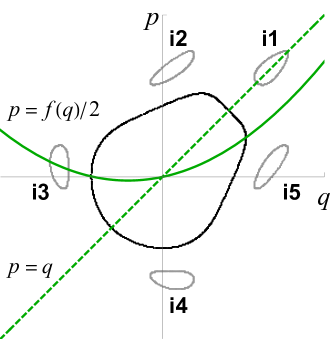
Figure 2: Two constant level sets $\mathcal{K}(p,q)=\mathrm{const}$ for the chaotic Hénon map, $f(p)=a\,p+b\,p^{2}$. The black curve shows a closed trajectory encompassing the origin and the gray curves show a set of islands (i.e. under iterations, points hop from island to island covering the closed gray curves labeled i1 – i5). While the first (reflection) symmetry is quite obvious from the figure, we will focus on the second one. The upper branch of the blue curve, $\Phi(q)$, is vertically equidistant from the lower branch, $\Phi^{-1}(q)$. Island i3 satisfies the second symmetry in the same manner as does the blue curve. Islands i1 and i2 satisfy the symmetry in a sense that they are vertical reflections of islands i5 and i4, respectively (e.g. the lower part of i1 is equidistant from the upper part of i5 and the upper part of i1 is equidistant from the lower part of i5). The dashed and solid green lines are the first and second symmetry lines.

III 1-piece maps

In this section, we will consider mappings in the MH form with $f$ being a simple linear function, $f(q)=k\,q$. We will refer to such mappings as 1-piece maps or mappings with linear force function, purposely avoiding the term “linear map.” We will reserve the term linear map (in contrast to nonlinear map) in order to refer to independence of dynamics on amplitude (i.e. rotation number is independent on amplitude for all stable trajectories); mappings in the MH form with nonlinear force function can possess linear dynamics. In order to avoid confusion, we will follow the terminology established above. As we will see, all 1-piece maps are integrable and linear.

III.1 Polygon maps with integer coefficients

According to crystallographic restriction theorem Bamberg et al. (2003); Kuzmanovich and Pavlichenkov (2002), if $A$ is an integer $2\times 2$ matrix and $A^{n}=I_{2}$ for some natural $n\in\mathbb{N}$, where $I_{2}=\mathrm{diag}\,(1,1)$ is an identity matrix, then the only possible solutions have periods $n=1,\,2,\,3,\,4,\,6$, which corresponds to 1-,2-,3-,4- and 6-fold rotational symmetries. Transformations with a period $n=1,2$ are simply $\pm I_{2}$, which can be considered as special cases of rotation of the plane, $\mathrm{Rot}(\theta)$, through the angles equal to $\theta=0$ or $\pi$ respectively. Three other cases, $n=3,4,6$, are given by mappings in the MH form

$$\begin{array}[]{ll}\alpha:\quad\begin{cases}q^{\prime}=p,\\ p^{\prime}=-q-p\end{cases}\end{array}\qquad\qquad\beta:\quad\begin{cases}q^{\prime}=p,\\ p^{\prime}=-q\end{cases}\qquad\qquad\gamma:\quad\begin{cases}q^{\prime}=p,\\ p^{\prime}=-q+p\end{cases}$$

further referred to as $\alpha$, $\beta$ and $\gamma$ respectively, and, with invariant polygons being concentric triangles, squares and hexagons (see Fig. 3).

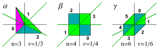
Figure 3: Integer mappings with linear force function and polygon invariants $\alpha$, $\beta$ and $\gamma$ (we use the same naming convention as Ref. Cairns et al. (2014, 2016)). Note that the invariant triangle was modified in order to satisfy both symmetries. Each figure shows one invariant polygon, with each colored region $i$ being mapped to region $i+1$. Here $n$ is the period and $\nu$ is the rotation number of the map, which represents the average increase in the angle per map iteration. The dashed and solid dark green lines show the first and second symmetry lines.

III.2 Fundamental polygons of the first kind

In order to understand the nature of invariant polygons from crystallographic restriction theorem, we first will consider a more general 1-piece map in the MH form

$$\begin{array}[]{l}q^{\prime}=p,\\[5.69046pt] p^{\prime}=-q+k\,p,\end{array}$$ (3)

where parameter $k\in\mathbb{R}$ is not restricted to integers. This map is known to be integrable with quadratic invariant of motion McMillan (1971)

$$\mathcal{K}(p,q)=p^{2}-k\,p\,q+q^{2}.$$

Mapping (3) is unstable for $|k|>2$, that results in level sets of the invariant being hyperbolas. On the other hand, the mapping is stable for $|k|<2$ with level sets corresponding to a family of concentric ellipses, see Fig. 4. Within the parameter range corresponding to stable maps, the rotation number $\nu$ is independent of the amplitude and given by $\nu=\arccos(k/2)/(2\pi)$.

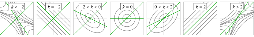
Figure 4: Constant level sets of invariant for 1-piece map in the MH form, $\mathcal{K}(p,q)=p^{2}-k\,p\,q+q^{2}=\mathrm{const}$ . For $|k|<2$ the level sets are ellipses, for $|k|>2$ the level sets are hyperbolas and for $|k|=2$ they are parallel lines. The dashed and solid green lines are the first and second symmetry lines.

Thus, one can see that if $\arccos(k/2)$ is incommensurate with $\pi$, the motion is quasi-periodic, and according to the Poincaré recurrence theorem, iterations starting from the initial condition $(q_{0},p_{0})$ will result in points densely covering the ellipse $\mathcal{K}(p,q)=\mathcal{K}(p_{0},q_{0})$. However, if $\arccos(k/2)$ is commensurate with $\pi$, motion is strictly periodic and $\nu$ becomes a rational number. As a result, point $(q_{0},p_{0})$ will return to its initial position after a finite number of iterations and will not depict an ellipse. In fact, linear mappings with rational $\nu$ are more than integrable, they posses superintegrability, meaning that they have more than one functionally independent invariant of motion $\mathcal{K}(p,q)$.

For example, for each map with rational $\nu\in\mathbb{Q}$, one can construct two sets of polygon invariants by iterating an initial point starting on the first, $p=q$, or second, $p=k\,q/2$, symmetry lines and using iterations as vertices (Fig. 5). We will refer to such polygons as first and second sets of fundamental polygons of the first kind; first or second sets refer to the position of the initial point on first or second symmetry lines respectively, and “the first kind” refer to the fact that the force function consists of one piece only. In the case of even period, two sets of polygons are actually different while for odd period sets, polygons are identical up to rotation by an angle $\pi$, $(q,p)\to(-q,-p)$. In the former case, the first set of polygons has no vertices on the second symmetry line (and two vertices on the first symmetry line) while the second set has no vertices on the first symmetry line (and two vertices on the second). In the latter case, both sets of polygons have a single vertex on each symmetry line.

The only integer values of $k$ corresponding to stable mappings ($|k|<2$) are $k\in\{-1,0,1\}$. For each integer value of parameter $k_{1}$, the value of $\arccos(k/2)$ (respectively $2\pi/3$, $\pi/2$ and $\pi/3$) is commensurate with $\pi$, thus proving that maps $\alpha$, $\beta$ and $\gamma$ are the only stable 1-piece maps in the MH form with integer coefficients.

In addition, for $|k|=2$ invariant level sets are straight lines. We will denote these mappings as “a” for $k=2$ and “b” for $k=-2$. While being unstable, both maps have polygonal chains (connected series of line segments, in this case just line itself) as its invariant. In the following sections, we will see that unstable and stable polygon maps can be combined together to form more complicated systems.

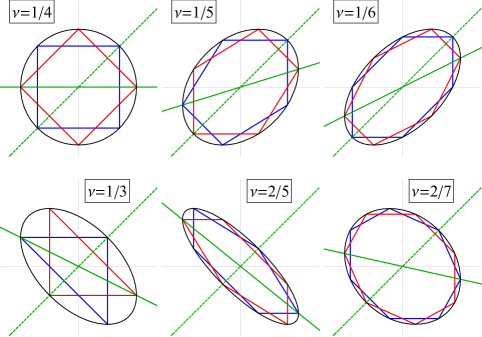
Figure 5: Fundamental polygons of the first kind for different values of rotation number $\nu$. Each plot shows the invariant ellipse $\mathcal{K}(p,q)=p^{2}-k\,p\,q+q^{2}=\mathrm{const}$ (black) and two invariant fundamental polygons inscribed into it (blue and red). The dashed and solid green lines correspond to the first and second symmetry lines.

IV 2-piece maps

IV.1 Linear mappings

IV.1.1 Polygon maps with integer coefficients

Another remarkably interesting result is given by CNR Theorem (Cairns, Nikolayevsky and Rossiter Cairns et al. (2014, 2016)). Suppose that $\mathcal{M}$ is a periodic continuous mapping of the plane that is a linear transformation with integer coefficients in each half plane $q\geq 0$ and $q<0$. Then $\mathcal{M}$ has a period

$$n=1,2,3,4,5,6,7,8,9\text{ or }12.$$

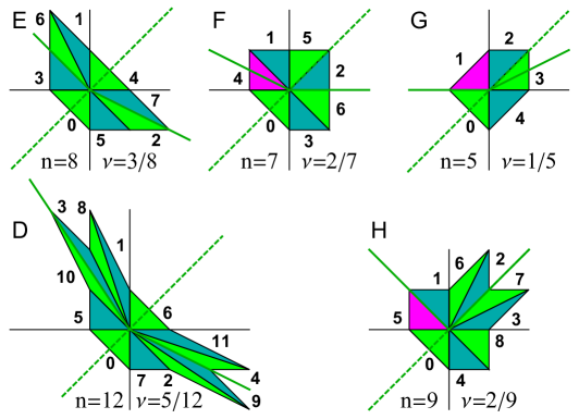
Figure 6: Integer mappings with 2-piece force function and polygon invariants D – H (named after Cairns et al. (2014)). Each figure shows one invariant polygon, with each colored region $i$ being mapped to the region $i+1$. Here $n$ and $\nu$ are the period and rotation number of the map. The solid and dashed dark green lines show the second and first symmetry lines.

All maps discovered by Cairns and others are in the MH form with force function consisting of two linear segments

$$f(q)=q\times\begin{cases}k_{1},&q<0,\\ k_{2},&q\geq 0.\end{cases}$$ (4)

In addition to previously described 1-piece maps (trivial cases $k_{1}=k_{2}$) with $n=1,2,3,4,6$, now we have 5 more mappings with $n=5,7,8,9$, Fig. 6. These maps are stable, linear and integrable, with polygons being their invariant sets, and denoted with capital Latin letters D – H. Note how Cairns, Nikolayevsky and Rossiter rediscovered Knuth map, H, from the first principles.

IV.1.2 Fundamental polygons of the second kind

Similar to the case of 1-piece mappings, in order to understand the origin of polygon invariants we should consider a less restricted map, corresponding to force function (4):

$$\begin{array}[]{l}\displaystyle q^{\prime}=p,\\[5.69046pt] \displaystyle p^{\prime}=-q+\frac{k_{1}+k_{2}}{2}\,p+\frac{k_{2}-k_{1}}{2}\,|p|,\end{array}$$ (5)

where parameters $k_{1,2}\in\mathbb{R}$. This is a very nontrivial dynamical system considered in great details in Beardon et al. (1995); Lagarias and Rains (2005a, b, c). Here, we will provide some results contributing to our understanding of polygon maps.

• Map (5) is integrable.

• Map (5) is linear, i.e., there is no dependence of the rotation number on the amplitude. Since we are free to choose units of $p$ and $q$, using scaling transformation ($\epsilon>0$)

  $$\begin{array}[]{l}\displaystyle q^{\prime}=\epsilon\,q,\\[5.69046pt] \displaystyle p^{\prime}=\epsilon\,p,\end{array}$$

  one can reconstruct dynamics on any ray of initial conditions (starting at the origin) from a single trajectory.

• The invariant of motion is a combination of segments of ellipses, straight lines or hyperbolas “glued” together and defined by $C_{1}p^{2}+C_{2}p\,q+C_{3}q^{2}=\mathrm{const}$. In the plane of parameters $(k_{1},k_{2})$ there are lines of constant topology. Along these lines, the number of segments remains constant.

• Dynamics of map (5) can be either stable or unstable depending on the values of $k_{1,2}$, that creates a nontrivial fractal area on the stability diagram (see Ref. Beardon et al. (1995) for more details). While we are not considering the fine structure of the fractal area, we would like to note that all pairs $(k_{1},k_{2})$ resulting in stable mappings are within the area defined by (Fig. 7)

  $$p,q<2\qquad\land\qquad p\,q<4\quad\mathrm{for}\quad p,q<0.$$

  Stable maps are either periodic when the rotation number $\nu$ is rational or quasi-periodic for irrational $\nu$.

  

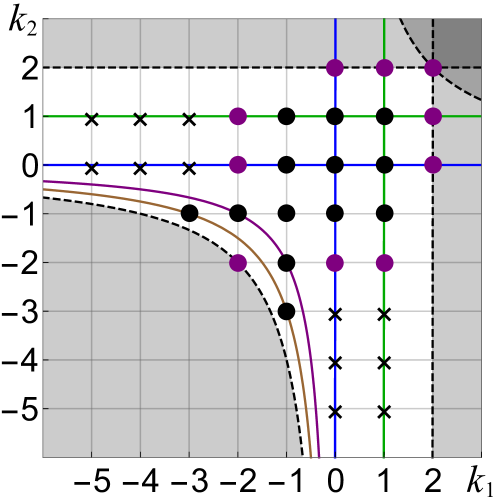
  Figure 7: The plane of parameters $(k_{1},k_{2})$ for 2-piece maps. The dashed lines show the area of global stability, $p,q<2\,\land\,p\,q<4$: the map can be stable (but not necessarily) only within the area of stability, shown in white. The solid curves show all lines of “constant topology” passing through integer nodes $(k_{1},k_{2})\in\mathbb{Z}^{2}$ within the stable zone: the red line corresponds to a single ellipse $k_{1}=k_{2}$, blue lines corresponds to two ellipses (McMillan beheaded and two-headed ellipse) $k_{1,2}=0$, green lines refer to three ellipses defined by $k_{1,2}=1$ and purple and brown hyperbolas are $k_{1}k_{2}=2$ and $k_{1}k_{2}=3$ respectively. Integer nodes corresponding to stable mappings with polygon invariants are shown in black, unstable mappings with an invariant being a polygonal chain in purple, and the remaining integer nodes within the global region of stability are shown with crosses (unstable maps with invariant consisting of hyperbolas).

• For example, the simplest case corresponds to the family of 1-piece maps, $k_{1}=k_{2}$, (red line in Fig. 7). As we learned above, in this case the phase space consists of only one ellipse (or two sets of hyperbolas conjugate to each other) defined by $\mathcal{K}(p,q)=p^{2}-k_{1}p\,q+q^{2}$. As we move along the line $k_{1}=k_{2}$, ellipses bifurcate into hyperbolas at $k_{1}=|2|$ and trajectories lose stability.

  Next line of constant topology is given by $k_{2}=0$ and line $k_{1}=0$ corresponding to family of twin maps, see blue solid lines in Fig. 7. This is the aforementioned beheaded and two-headed ellipses discovered by McMillan with invariant defined by two ellipses glued together:

  $$\mathcal{K}(p,q)=\left\{\begin{array}[]{l}p^{2}+k_{1}p\,q+q^{2},\qquad p,q\geq 0,\\[5.69046pt] p^{2}-k_{1}p\,q+q^{2},\qquad\mathrm{otherwise}.\end{array}\right.$$

  Here is his explanation on how this map works: In an earlier paragraph a promise was made that cases could be constructed with boundaries that more than double valued. I shall now fulfill the promise by describing a procedure by which this can be done. Take any known case with a center of symmetry at the origin, and erase the part of the boundary lying in the $+$, $+$ quadrant. Replace $f(q)$ by $f(q)=0$ to the right of the origin. Fill in the erased part of the boundary by reflecting the part in the $+$, $-$ quadrant about the $q$-axis. The resulting completed boundary is an invariant under the transformation with the original $f(q)$ to the left of the boundary, and $f(q)=0$ to the right. Starting with ellipses, we can get beheaded ellipses (first row of Fig. 8, case $0<k_{1}<2$) or double headed ellipses (first row of Fig. 8, case $-2<k_{1}<0$), and here we see a four-valued function acting as an invariant boundary. Note that in order to have only two ellipses being invariants of motion, the second ellipse have to be added to the $+$, $+$ quadrant (or to $-$, $-$ quadrant for twin maps with $k_{1}=0$). Otherwise, an addition of an ellipse into the $+$, $-$ quadrant will result in its reflection in the quadrant $-$, $+$ (due to the first symmetry line $p=q$) making number of ellipses equal to three.

  

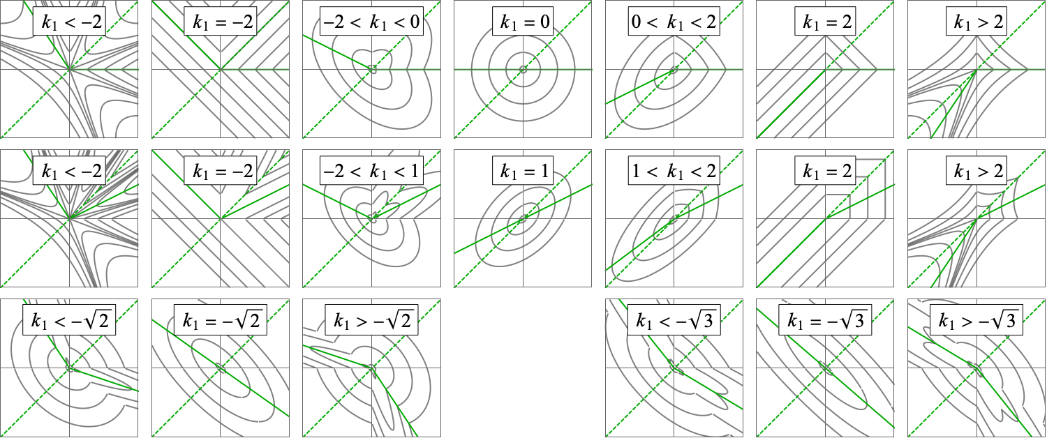
  Figure 8: Invariant level sets along lines of constant topology for a 2-piece map in the MH form. The first and second rows illustrate the transformation of the invariant for cases $k_{2}=0$ and $k_{2}=1$ (blue and green lines in Fig. 7). The three left plots in the third row show bifurcation along hyperbola $k_{1}k_{2}=2$ and the three right plots are for $k_{1}k_{2}=3$ (purple and brown hyperbolas in Fig. 7). The solid and dashed green lines are the second and first symmetry lines.

  In the case when the second segment of the force function has zero slope, $k_{2}=0$, the map in Eq. (5) is stable for $|k_{1}|<2$ (see first row of Fig. 8). For the slopes $k_{1}=\pm 2$ the invariant level sets become polygonal chains with 1- and 3-fold symmetries respectively. When stable, the rotation number is given by

  $$\nu=\frac{\arccos(k_{1}/2)}{\pi+2\,\arccos(k_{1}/2)}.$$

  As in the case $k_{1}=k_{2}$, when $\arccos(k/2)$ is commensurate with $\pi$, we have a rational rotation number $\nu\in\mathbb{Q}$ resulting in a periodic map. The only integer values of $k_{1}$ satisfying this condition are $k_{1}\in\{-1,0,1\}$ (mappings F, $\beta$ and G respectively).

  In fact, this line of constant topology is just one of many defined by $k_{2}=2\,\cos(\pi/n)$ for $n\geq 2$. On each line the map is stable for $|k_{1}|<2$, it produces a polygonal chain as invariant for $k_{1}=\pm 2$ and when stable has a rotation number

  $$\nu=\frac{\arccos(k_{1}/2)}{\pi+n\,\arccos(k_{1}/2)}.$$

  Along each line of constant topology the invariant consists of $n$ ellipses (hyperbolas) with $n-1$ of them being in the first quarter.

  Among these lines there is another line that we should focus on: case $n=3$ with $k_{2}=1$ (and twin $k_{1}=1$). As we can see, in addition to line $k_{2}=0$, this is the only line with integer $k_{1}$. The invariant of motion is

  $$\mathcal{K}(p,q)=\left\{\begin{array}[]{l}p^{2}-(2-k_{1})(p\,q-q^{2}),\qquad p,q\geq 0\,\land\,p>q,\\[5.69046pt] (2-k_{1})(p^{2}-p\,q)+q^{2},\qquad p,q\geq 0\,\land\,p<q,\\[5.69046pt] p^{2}-k_{1}p\,q+q^{2},\qquad\qquad\quad\,\mathrm{otherwise},\end{array}\right.$$

  second row of Fig. 8. From this line we have two more mappings with polygonal chain ($k_{1}=\pm 2$) and three periodic maps with integer coefficients ($k_{1}=-1,0,1$, i.e maps $\alpha$ F and H).

• As one can notice, lines $k_{1}=k_{2}$ and $k_{1,2}=0,1$ are covering most of integer nodes $(k_{1},k_{2})\in\mathbb{Z}^{2}$ within the area of global stability (see Fig. 7). The remaining nodes belongs to two lines of constant topology from the family given by $k_{1}k_{2}=4\cos^{2}(\pi/(2n))$ with $k_{1,2}<0$ and $n\geq 2$. Those lines are for $n=2$ and 3. Along those lines map is always stable and periodic with the rotation number $\nu=(2\,n-1)/(4\,n).$ The invariant of motion is glued of $(2\,n-1)$ ellipse: the central ellipse, $(n-1)$ ellipses in II quadrant, and another $(n-1)$ in IV quadrant (placed symmetrically with respect to $p=q$). For example, for $n=2$ the invariant is

  $$\mathcal{K}(p,q)=\left\{\begin{array}[]{l}p^{2}-(\frac{4}{k_{1}}-k_{1})\,p\,q+(\frac{4}{k_{1}^{2}}-k_{1})\,q^{2},\qquad p,q\geq 0\,\land\,p>q,\\[5.69046pt] (\frac{4}{k_{1}^{2}}-k_{1})\,p^{2}-(\frac{4}{k_{1}}-k_{1})\,p\,q+q^{2},\qquad p,q\geq 0\,\land\,p<q,\\[5.69046pt] p^{2}-k_{1}p\,q+q^{2},\qquad\qquad\qquad\qquad\quad\,\,\mathrm{otherwise}.\end{array}\right.$$

  Third row of Fig. 8 illustrates this case. For $k_{1,2}=-1$ from lines $n=2,3$ we have two remaining periodic maps with integer coefficients, E and D.

Thus, similarly to the case of the 1-piece map (degenerate line $k_{1}=k_{2}$), we can define fundamental polygons of the second kind: for each line of constant topology, its stable maps with a rational rotation number are degenerate and have more than one invariant of motion including polygons. In contrast to the case $k_{1}=k_{2}$, when we had two sets of polygons, now we only have only a single set of fundamental polygons. These polygons have two vertices on the second symmetry line for maps with an even period or a single vertex on both symmetry lines for odd periods. Fig. 9 shows a few examples of this degeneracy illustrating fundamental polygons of the second kind inscribed in alternative invariant set of ellipses. Note that the first example is for Brown-Knuth map showing an alternative three-headed ellipse which is also an invariant of motion.

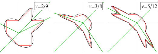
Figure 9: Shapes of fundamental polygons of the second kind corresponding to different families of maps represented in Fig. 7. Each plot shows invariant ellipses (black) and invariant polygons inscribed into it (red). From left to right: line $k_{2}=1$ for $k_{1}=-1$ (Brown-Knuth map, H), line $k_{1}k_{2}=2$ for $k_{1}=-1$, line $k_{1}k_{2}=3$ for $k_{2}=-3$ (map E). The dashed and solid green lines correspond to the first and second symmetry lines.

IV.1.3 Ingredients of mappings with polygon invariant

Hereby, one can see that there is one condition and two mechanisms determining polygon shapes (including unstable mappings with invariant level set being connected series of line segments — non-intersecting polygonal chains). The condition is that the force function $f$ should be in a piecewise linear form that follows from the second symmetry: the sum of vertically opposed polygon sides is proportional to the value of the force function. Two mechanisms are:

• Superintegrability in linear maps. Rational rotation number causes degeneracy when more than one invariant of motion exists, including polygons (e.g. fundamental polygons of the first and second kind).

• Loss of stability. Ellipses are transitioned to hyperbolas via the straight lines in linear 2-piece maps, e.g. see cases $|k_{1}|=2$ for first two rows in Fig. 8.

These mechanisms are respectively responsible for stable and unstable polygons. As we will see further, more complicated nonlinear mappings with polygon invariants can be constructed, but at lower ($(q,p)\rightarrow 0$) or higher amplitudes ($(q,p)\rightarrow\infty$), they reduce to one of the already described transformations; we will observe that both mechanisms can be combined in one map resulting in very nontrivial dynamics. Below, in Fig. 10 we illustrate all integer linear mappings with 2-piece force function and polygon invariants (stable and unstable).

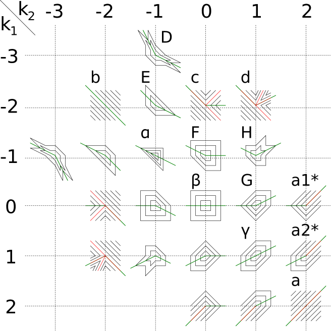
Figure 10: Integer linear mappings with 2-piece force function and polygon invariants (stable and unstable maps). The black polygons (or polygonal chains for unstable mappings) show constant level sets of the invariant, red level sets are separatrix for unstable mappings with stable periodic dynamics, and the green line is the second symmetry line.

IV.2 Nonlinear mappings

Here we begin our exploration of nonlinear symplectic mappings. So far we considered only mappings with force function in the form (4). The simplest modification we can make is to add a constant shift parameter, $d$:

$$f(q)=\frac{k_{1}+k_{2}}{2}\,q+\frac{k_{2}-k_{1}}{2}\,|q|+d.$$

The map becomes nonlinear and we can not reconstruct dynamics along the ray of initial conditions using scaling transformation $(q,p)\to\epsilon(q,p)$, $\epsilon>0$. Instead, now we have a choice of natural units $\epsilon=d$, and one can show that without loss of generality for 2-piece maps, $d$ can be restricted to $\pm 1$ or 0.

Introduction of $d$ not only adds the dependence on amplitude, but might result in a loss of integrability causing chaotic behavior. A famous example is the Gingerbreadman Devaney (1984) map — a chaotic two-dimensional map in the MH form with $f(q)=|q|+1$ (see first plot in Fig. 11). The remarkable property of this map is that some invariant tori survived perturbation and after deformation remained polygons. The chaotic dynamics is sectioned by concentric polygons making this map the simplest model for area-preserving twist mappings with zones of instability. It shares many properties of the smooth mappings and has an advantage of having an exact arithmetic on rational numbers. Another mapping we would like to mention here is the Rabbit map for $f(q)=|q|-1$. To the best of our knowledge this map has not been mentioned before, but we are certain that Robert Devaney, the discoverer of Gingerbreadman, knew about it due to the close connection between the maps (second plot in Fig. 11).

IV.2.1 Zoo mappings

After reading the article of Cairns, Nikolayevsky and Rossiter Cairns et al. (2014), our first idea, which predetermined discoveries made in this article, was to produce objects similar to Devaney map using newly discovered mappings D – G. First we tried mapping D, and amazingly it worked! We introduce two new dynamical systems, the Octopus and the Crab mappings for $f(q)=|q|-2q\pm 1$ respectively Zolkin and Nagaitsev (2017) (last two plots in Fig. 11). Informally, we grouped them together with Rabbit and Gingerbreadman, and, called them zoo maps. Mappings are again chaotic and “sectioned” by infinitely many concentric invariant polygons. Basic dynamics of these maps is described in the caption to Figure 11 and dynamical properties of invariant polygons are listed in Table 14 (Appendix D).

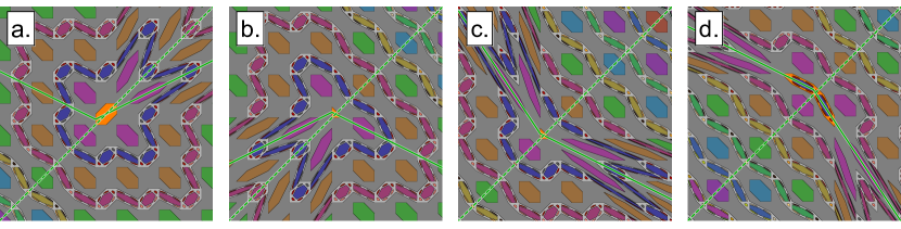
Figure 11: Zoo maps: Gingerbreadman (a.), Rabbit (b.), Octopus (c.) and Crab (d.) mappings. The light and dark gray areas represent alternating zones of instability which are sectioned by two families of concentric invariant polygons resembling animals. Within each zone of instability there are three different scenarios. First, orbits that result from initial conditions $(q_{0},p_{0})$ within any gray zone such that both $q_{0},p_{0}\in\mathbb{Q}$. Those are stable orbits with an exact periodic motion and rational rotation number resulting in an invariant set of points. The second scenario includes all other initial conditions within the gray zones with any or both $q_{0},p_{0}$ being irrational, $q,p_{0}\in\mathbb{R}\setminus\mathbb{Q}$. Those are chaotic orbits never returning to initial conditions and densely covering the zone of instability. The third and last scenario is for any initial condition within the colored regions of phase space. Those are chains of linear islands; the initial condition from these regions of phase space hops from island to island of the same group (each group is shown with its own color related to the relative orbit period). Such initial condition returns to itself and the motion is strictly periodic with the rotation number being mode-locked within the island. To view an “animal” you must rotate each image 135 degrees clockwise.

IV.2.2 Nonlinear integrable maps with polygon invariants

Map	$\nu_{0}$	$\nu_{1}$	$J_{1}$	$J_{1}^{\prime}$
b0	$\frac{1}{2}$	$\frac{1+3x}{2+8x}$	$4\,\!x^{2}+2x$	$\frac{3}{2}x^{2}+x$
$\alpha$1	$\frac{1}{3}$	$\frac{1+3x}{3+8x}$	$4\,\!x^{2}+3x+\frac{1}{2}$	$\frac{3}{2}x^{2}+x+\frac{1}{6}$
$\alpha$2	$\frac{1}{3}$	$\frac{1+2x}{3+7x}$	$\frac{7}{2}x^{2}+3x+\frac{1}{2}$	$x^{2}+x+\frac{1}{6}$
$\beta$1	$\frac{1}{4}$	$\frac{1+2x}{4+7x}$	$\frac{7}{2}x^{2}+4x+1$	$x^{2}+x+\frac{1}{4}$
$\beta$2	$\frac{1}{4}$	$\frac{1+x}{4+5x}$	$\frac{5}{2}x^{2}+4x+1$	$\frac{1}{2}x^{2}+x+\frac{1}{4}$
$\gamma$1	$\frac{1}{6}$	$\frac{1+x}{6+5x}$	$\frac{5}{2}x^{2}+6x+3$	$\frac{1}{2}x^{2}+x+\frac{1}{2}$

Table 1: Dynamical properties of integer nonlinear integrable mappings with polygon invariants and 2-piece force function. Here $\nu_{0}$ is the rotation number in the inner linear layer, $\nu_{1}$, $J_{1}$ and $J^{\prime}_{1}$ are respectively rotation number, action and partial action in the outer nonlinear layer, $x$ is the linear amplitude in a nonlinear layer defined as horizontal or vertical distance from separatrix to the trajectory under consideration.

When $d=\pm 1$, not all mappings experience chaotic behavior like Gingerbreadman or zoo maps. Unexpectedly, transformations E, F and G produced nonlinear integrable systems with polygon invariants if the vertical shift parameter $d$ is added Zolkin and Nagaitsev (2017) (see Fig. 12). Since $d\neq 0$, fixed point moves from the vertex to one of the linear pieces (depending on a sign of $d$) of the force function. As a result, the area of mode-locked motion around fixed point is formed with invariant level sets being triangles, squares, hexagons or line segment $p=-q$ with period 2 for map b0. For larger amplitudes, the motion is still integrable, but rotation number becomes amplitude dependent (trajectories shown in blue). The inner linear and outer nonlinear layers are separated by separatrix matching dynamics (shown in red). Dynamical properties for all mappings are listed in Table 1 as functions of amplitude along $q$-axis $x$, and, methods for calculation of rotation number as well as action-angle variables are provided in Appendix A.

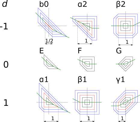
Figure 12: Integer nonlinear integrable maps with polygon invariants and 2-piece force function. The top and bottom rows of the figures show level sets of the invariant for $d=\mp 1$. The middle row shows cases for $d=0$, and, in each column the transformations have the same slopes $k_{1,2}$ as for $d=0$ (see Fig. 10); note that the invariant level set of the outer nonlinear layer at the large amplitude is asymptotic to the level set of the corresponding map. The black (blue) level sets are linear (nonlinear) trajectories. The red level sets represent the separatrix isolating the inner linear from the outer nonlinear layers. The green line shows the second symmetry line, $p=f(q/2)$.

V Machine-assisted discovery of integrable maps with polygon invariants

After discovering 6 nonlinear polygon maps shown in Fig. 12 and performing few more numerical experiments, we realized that the force function can be further generalized to have $n>2$ linear segments, potentially producing new families of integrable systems. In order to automate the search, we designed a relatively simple algorithm that finds integrable mappings based on the analysis of individual trajectories; first, we verified some of its principles in Zolkin et al. (2019), and then we significantly modified it and performed an extensive search. The detailed pseudo-code of the search algorithm is presented in Appendix B while its Python implementation is available at github.com/yourball/polygon-maps. The algorithm is illustrated via flowchart in Fig. 13 and its blocks with processes/decisions are described below.

1. Input We decided to focus on piecewise linear forces with integer coefficients, $f(q,\mathbf{k},\mathbf{l},d)$ with integer vectors $\mathbf{k},\mathbf{l}$ and $d$. While we performed a scan only for integer slopes $\mathbf{k}$, we were able to analytically generalize some of the results for more general values of the shift parameter $d\in\mathbb{R}$ and lengths of segments $\mathbf{l}\in\mathbb{R}^{+}$.

2. Fixed point In order for a map to be stable, i.e. all phase space orbits are bounded, it should have at least one fixed point $\zeta^{*}=(q^{*},p^{*})$. Mappings that do not have a fixed point, $\forall\,q\in\mathbb{R}:\,q\neq f(q)/2$, are out of scope.

3. Tracking If map is selected, we trace out its orbits $\vec{\zeta}=(\zeta_{1},\ldots,\zeta_{N})$ for different initial conditions $\zeta_{0}=(q_{0},\,p_{0})$.

4. Stability Mappings with fixed point still can have unstable trajectories at larger amplitudes. If for some initial condition we detect an unbounded growth of the radial distance from the fixed point, $\exists\,i:\,\,|\zeta_{i}-\zeta^{*}|>r_{\mathrm{max}}$, the map is excluded from further analysis.

5. Ordering At the next stage the points of each individual trajectory are ordered according to their polar angle $\phi=\arctan{\left[(p-p^{*})/(q-q^{*})\right]}$, such that the angle $\phi$ is monotonically increasing. After arranging trajectory points according to $\phi$ we join consecutive points resulting in an orbit polygon.

6. Vertex count In order to count the number of vertices, $V$, for each orbit polygon we use scalar products of two vectors build on three consequent points ($\mathbf{v}_{1}=\zeta_{i}-\zeta_{i-1}$ and $\mathbf{v}_{2}=\zeta_{i+1}-\zeta_{i}$),

   $$V=\sum_{i}\theta(\alpha_{i}-1),\qquad\qquad\alpha_{i}=\frac{\mathbf{v}_{1}\cdot\mathbf{v}_{1}}{|\mathbf{v}_{1}||\mathbf{v}_{2}|},$$

   where $\theta(x)=\mathbf{1}_{x>0}$ is a Heaviside step function. In numeric experiments, when $\mathbf{v}_{1}\parallel\mathbf{v}_{2}$, the normalized scalar product might be slightly different from unity, so a small cutoff parameter should be introduced, $\epsilon<\left|(\mathbf{v_{1}}\cdot\mathbf{v_{2}})/(|\mathbf{v_{1}}||\mathbf{v_{2}}|)-1\right|$.

7. Vertex cutoff At the final stage we are left with stable integrable or chaotic maps which we would like to separate. The key insight is that we are looking for transformations with all invariant tori being polygons and assume that the phase space consists of concentric layers; in each layer the orbit polygons have the same finite number of vertexes which remains bounded when increasing the number of iterations $N\to\infty$. Conversely, for a chaotic trajectory the number of vertices linearly grows with the number of iterations, $V=\mathcal{O}(N)$. Such drastic difference in the growth of $V$ with the iteration number allows us to automatically separate between the two cases. In numeric experiment we check that for all initial conditions the number of vertices is bounded by some cutoff parameter, $V<V^{\mathrm{cutoff}}\leq N$.

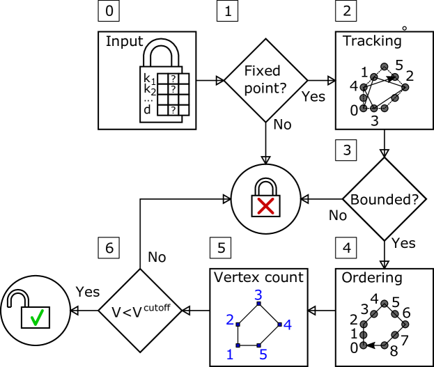
Figure 13: Flowchart representing the machine-assisted discovery of integrable maps. The algorithm verifies if the map defined by the input (0.) is integrable with the invariants being concentric polygons. If the map has a fixed point (1.), the algorithm performs tracking for different initial conditions (2.), and, if all orbits are bounded (3.) it proceeds to the construction of orbit polygons via ordering (4.). Finally, after counting the number of vertices $V$ (5.), if for each polygon $V<V^{\mathrm{cutoff}}$, the map is sent for analytic verification. The search process terminates when any conditional operation is false (NO).

In addition, for each mapping found by the search algorithm, we manually verify the McMillan integrability condition, thus rigorously proving their integrability. Although the search algorithm described here is quite powerful, there are some caveats to bear in mind:

• Maps with strongly non-convex layers of polygon invariants can be missed by the algorithm. In cases when the orbit polygon is not convex with respect to the fixed point $(q^{*},\,p^{*})$, the points of the trajectory can not be ordered according to the polar angle. While we do not have a particular example, we should keep it in mind.

• Inside integrable nonlinear layers fibrated with polygons there are two types of orbits: those with rational and those with irrational rotation numbers. The latter are quasi-periodic with entire polygon being densely covered. On the other hand, the former are strictly periodic with orbit visiting only finite number of points, thus potentially showing a smaller number of vertexes. In Appendix A we show that all rotation numbers within a layer are in the form $\nu(q_{0})=(\alpha+\beta\,q_{0})/(\gamma+\delta\,q_{0})$, where $\alpha,\,\beta,\,\gamma$ and $\delta$ are integer parameters. In order to avoid periodic orbits which complicate analysis, we can add a small irrational perturbation $\eta$ to all initial conditions, $q_{0}\rightarrow q_{0}+\eta$. In fact, from this formula one can see that in numeric experiments all observed orbits are periodic but this is not a problem as long as period is sufficiently large compare to the number of polygon sides, so points of orbit visit all sides of polygon covering them densely enough.

• Finally, while we’ve been only looking for maps with invariant layers being concentric polygons, while phase space can involve polygon islands. In the case of completely mode-locked islands (linear islands) with all orbits visiting each island only once, our algorithm will successfully handle this case. But in the case of nonlinear islands (i.e. a trajectory visits sequentially each island under iterations and traces out invariant tori around centers of islands) our algorithm indeed will fail; as in the case of non-convex polygons, points of orbit can not be arranged by polar angle since now they are a multiple valued function.

We performed the search for 3- and 4-piece integer force functions using our algorithm across a wide range of the parameter values. The integer valued slopes of the segments of the force function are selected from the range $-10\leq k_{i}\leq 10$ and the shift parameter $-50\leq d\leq 50$. In the case of four-piece maps, the additional degree of freedom in the space of parameters corresponds to the ratio of the lengths of segments, $r\in[1/10,1/9,\ldots,1,2,\ldots,10]$. However, the search space can be further reduced when relying on our prior knowledge about properties of piecewise linear mappings with two segments. A generic $n$-piece mapping at small and large amplitudes reduces to a two-piece mapping. As illustrated in Fig. 10 two-piece mappings with integer slope coefficients and polygon invariants are confined to the parameter range $-3\leq k_{1,2}\leq 2$. Therefore the values of the slopes of the outer segments in mappings with polygon invariants are also restricted to $-3\leq k_{1,n}\leq 2$. Similarly, in the vicinity of the fixed point $(q^{*},\,p^{*})$ at small amplitudes $|q-q^{*}|\to 0$ and $|p-p^{*}|\to 0$, the mapping behaves as a single-piece or two-piece map, depending on whether the fixed point belongs to the segment of the force function or coincides with one of the vertexes separating adjacent segments. Therefore, in order to guarantee that the mapping has polygon tori in the vicinity of the fixed point, the range for the slope $k_{i}$ for the corresponding segment is also confined to the same range. The values of the shift parameter $d$ and the length ratio $r$ are less restrictive, because they are only responsible for the position of the fixed point. While we performed a scan only for integer $d$ and $r$ we were able to analytically generalize some of these results for $d,r\in\mathbb{R}$.

VI 3-piece maps

In order to construct more complex piecewise linear symplectic maps, one can add more segments to the force function $f$. When the number of segments is equal to three, we have four independent parameters: three slopes $k_{1,2,3}$ and a shift parameter $d$. By performing the rescaling of coordinates, one can see that without loss of generality, the length of the middle segment can always be assumed to be equal to one. In addition, unlike the case of 2-piece force function when $d=0,\pm 1$, now the shift parameter belongs to reals. Below, we will classify search results as isolated with respect to $d$ (finite set of integer values), discrete (all integer values, $d\in\mathbb{Z}$), and continuous (map is integrable for any $d\in\mathbb{R}$). Results of the machine-assisted search of new integrable maps are briefly summarized in Fig. 14 (the symmetry with respect to $k_{1}=k_{3}$ is due to “twin” mappings).

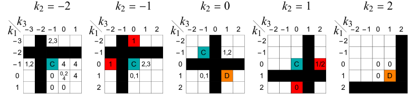
Figure 14: Integrable polygon mappings corresponding to a piecewise linear force function with three segments. Each table corresponds to its own value of $k_{2}$ and shows the value of the shift parameter $d$. Black cells represent degenerate cases when 3-piece force function becomes 2-piece ($k_{1}=k_{2}$ or $k_{2}=k_{3}$), white cells represent cases with isolated integer $d$ showing its values, orange cells represent mappings integrable for any integer $d\in\mathbb{Z}$ (“D”), cyan cells represent mappings integrable for continuous $d\in\mathbb{R}$ (“C”) and red cells represent unstable nonlinear polygon mappings where the numbers in the cell shows the values of $d$ corresponding to integrable maps.

VI.1 Isolated d

Integer integrable polygon mappings with 3-piece force function and isolated $d$ are shown in Fig. 15 and rotation numbers are provided in Table 2. As one can see, the addition of new pieces can stabilize previously unstable 2 pieces maps a (a1,$2^{*}$), b, c and d (respectively mappings a1–3, b1–3, c1–2 and d1–2). Mappings $\alpha$3, $\beta$4–5 and H1 can be seen as previously considered linear transformations ($\alpha$, $\beta$ and H) with outer layer of nonlinear stable trajectories determined by the new piece in the force function.

Something interesting can be observed for mappings b0.1, $\beta$3 and G1. For the map b0.1 we see that the inner and outer nonlinear layers are separated by a chain of islands. Unlike the “usual” chaotic chains observed in systems like Hènon Henon (1969) or Chirikov Chirikov (1969, 1979) mapping (where under iterations phase-space point jumps from island to island and trace out elliptic orbits around centers of islands), these are linear islands. They show true mode-locking similar to one observed in Arnold tongue Arnol’d (1961) or even more similar to Gingerbread man map Devaney (1984); when iterated, any initial condition within the chain returns exactly to the same position after visiting each island only once. Thus, the rotation number of the inner layer

$$\nu_{0}=\frac{\frac{1}{2}+3x}{1+8x},\qquad x\in[0,\frac{1}{2}],$$

and the one of the outer layer

$$\nu_{1}=\frac{4+5y}{10+12y},\qquad y\in[0,\infty),$$

where $x$ and $y$ represent the linear amplitudes, are matched on the outer and inner separatrices, respectively $x=\frac{1}{2}$ and $y=0$. They are equal to the rotation number inside the linear chain consisting of 5 islands

$$\nu_{0}(1/2)=\nu_{1}(0)=\frac{2}{5}.$$

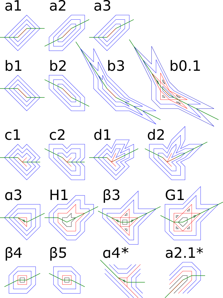
Figure 15: Integrable polygon mappings with 3-piece force function and isolated $d$. Black and blue lines correspond to linear and nonlinear invariant phase space trajectories, red lines are separatrices, and the thick green line is a second symmetry line, $p=f(q)/2$. Mappings b2 and $\beta$5 are also integrable for any $d\in\mathbb{R}$ and mappings a2 and $\beta$4 are also integrable for any $d\in\mathbb{Z}$. Mappings $\alpha 4^{*}$ and a2.$1^{*}$ are unstable and were missed by the search algorithm.

Map	$\nu_{0}$	$\nu_{1}$	$J_{1}$	$J_{1}^{\prime}$
a1	$0$	$\frac{x}{2+4x}$	$2x^{2}+2x$	$\frac{1}{2}x^{2}$
a2	$0$	$\frac{x}{2+6x}$	$3x^{2}+2x$	$\frac{1}{2}x^{2}$
a3	$0$	$\frac{x}{2+5x}$	$\frac{5}{2}x^{2}+2x$	$\frac{1}{2}x^{2}$
b1	$\frac{1}{2}$	$\frac{1+x}{2+4x}$	$2x^{2}+2x$	$\frac{1}{2}x^{2}+x$
b2	$\frac{1}{2}$	$\frac{1+2x}{2+6x}$	$3x^{2}+2x$	$x^{2}+x$
b3	$\frac{1}{2}$	$\frac{1+5x}{2+12x}$	$6x^{2}+2x$	$\frac{5}{2}x^{2}+x$
c1	$\frac{1}{3}$	$\frac{2+x}{6+4x}$	$2x^{2}+6x$	$\frac{1}{2}x^{2}+2x$
c2	$\frac{1}{3}$	$\frac{2+2x}{6+7x}$	$\frac{7}{2}x^{2}+6x$	$x^{2}+2x$
d1	$\frac{1}{4}$	$\frac{2+x}{8+5x}$	$\frac{5}{2}x^{2}+8x$	$\frac{1}{2}x^{2}+2x$
d2	$\frac{1}{4}$	$\frac{2+2x}{8+9x}$	$\frac{9}{2}x^{2}+8x$	$x^{2}+2x$
$\alpha$3	$\frac{1}{3}$	$\frac{1+x}{3+5x}$	$\frac{5}{2}x^{2}+3x+\frac{1}{2}$	$\frac{1}{2}x^{2}+x+\frac{1}{6}$
$\beta$3	$\frac{1}{4}$	$\frac{2+2x}{8+9x}$	$\frac{9}{2}x^{2}+8x+3$	$x^{2}+2x+\frac{3}{4}$
$\beta$4	$\frac{1}{4}$	$\frac{1+x}{4+6x}$	$3x^{2}+4x+1$	$\frac{1}{2}x^{2}+x+\frac{1}{4}$
$\beta$5	$\frac{1}{4}$	$\frac{1+2x}{4+6x}$	$3x^{2}+4x+1$	$x^{2}+x+\frac{1}{4}$
H1	$\frac{2}{9}$	$\frac{2+x}{9+5x}$	$\frac{5}{2}x^{2}+9x+\frac{9}{2}$	$\frac{1}{2}x^{2}+2x+1$
G1	$\frac{1}{5}$	$\frac{2+2x}{10+9x}$	$\frac{9}{2}x^{2}+10x+5$	$x^{2}+2x+1$

Table 2: Rotation numbers of the inner linear, $\nu_{0}$, and outer nonlinear layers, $\nu_{1}$, for integer integrable polygon mappings with 3-piece force function and isolated $d$. Last two columns show action, $J$, and partial action (Hamiltonian), $J^{\prime}$, in nonlinear layer. Parameter $x\in[0,\infty)$ is horizontal (vertical) distance from the separatrix to considered trajectory.

Note that polygons inside the chain of islands satisfy both symmetries as a level set of the entire group and are invariant under transformation; for each island, there is another one which is its vertical reflection with respect to the second symmetry line, and one reflected with respect to the main diagonal (unless the island is its own reflection with respect to the symmetry line). Due to the fact that dynamics inside the island chain is degenerate (all rotation numbers are the same), invariant contours can not be simply traced out in the numerical experiment by looking at the mapping iterations, but can be reconstructed from the symmetries in order to match the separatrices.

Mappings $\beta$3 and G1 don’t have an inner nonlinear layer, and the chain of islands is attached to a linear layer, so the entire combined phase space is mode-locked. As expected, the number of islands is equal to the period inside linear zone (4 for $\beta$3 and 5 for G1) and rotation numbers are $1/4$ and $1/5$ respectively.

Finally, two more mappings, $\alpha 4^{*}$ and $a2.1^{*}$, are shown at the end of the last row. These cases were not found by an algorithm, since the outer layer is unstable, and were constructed by authors using symmetries.

Map	$\nu_{0}$	$\nu_{1},\,J_{1},\,J_{1}^{\prime}$	$\nu_{\mathrm{isl}}$, $\#_{C}$	$\nu_{2},\,J_{2},\,J_{1}^{\prime}$
a2-$k,\,(k\geq 1)$	$\frac{1}{6},\,x\in[0,k]$	$\frac{k}{6k+y},\,y\in[0,1]$	$\frac{k}{6k+1},\,k$	$\frac{2k+z}{2(6k+1)+6z},\,z\in[0,\infty)$
		$\frac{1}{2}y^{2}+6ky$		$3z^{2}+2(6k+1)z+J_{1}(1)$
		$ky$		$\frac{1}{2}z^{2}+2kz+J_{1}^{\prime}(1)$
$\beta$4-1	—	$\frac{1}{5},\,y\in[0,1]$	$\frac{1}{5},\,1$	$\frac{2+z}{10+6z},\,z\in[0,\infty)$
$\beta$4-$k,\,(k>1)$	$\frac{1}{6},\,x\in[0,k-1]$	$\frac{k-1+y}{6(k-1)+5y},\,y\in[0,1]$	$\frac{k}{6k-1},\,k$	$\frac{2k+z}{2(6k-1)+6z},\,z\in[0,\infty)$
		$\frac{5}{2}y^{2}+6(k-1)y$		$3z^{2}+2(6k-1)z+J_{1}(1)$
		$\frac{1}{2}y^{2}+(k-1)y$		$\frac{1}{2}z^{2}+2kz+J_{1}^{\prime}(1)$

Table 3: Rotation number, $\nu_{i}$, action, $J_{i}$, and partial action, $J_{i}^{\prime}$, for the $i$-th layer of the integer integrable polygon mappings with 3-piece force function and discrete $d$. $\nu_{\mathrm{isl}}$ and $\#_{C}$ are the rotation number in mode-locked area and number of chains in group of linear islands, respectively.

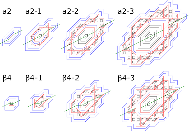
Figure 16: Integer integrable polygon mappings with 3-piece force function and discrete $d\in\mathbb{Z}$. Each row shows first 4 members of a family.

VI.2 Discrete d, (D)

Mappings a2 and $\beta$4 are integrable for any $d\in\mathbb{Z}$, forming two families of transformations with discrete parameter. Invariant level sets are shown in Fig. 16. The rotation number is provided in Table 3 and Fig. 17 shows it as a function of amplitude. Inner and outer layers become separated with chains of linear islands, with increment (or decrement) of $d$ from cases a2 and $\beta$4, and the number of chains increases linearly with $d$. On these groups of linear islands, the rotation number is again mode-locked.

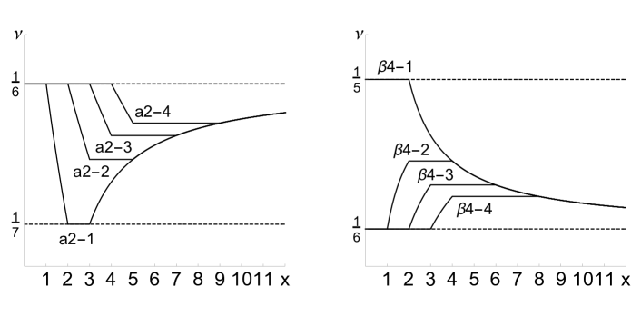
Figure 17: Rotation number $\nu$ as a function of amplitude $x$ (horizontal or vertical distance measured from fixed point to invariant polygon) for families of mappings a2-$k$ and $\beta 4$-$k$ with $k=1,\ldots,4$.

VI.3 Continuous d, (C)

In this subsection we present the last class of integer mappings with 3-piece force function which is integrable for $d\in\mathbb{R}$. Previously mentioned mappings b2 and $\beta$5 as well as two more, $\gamma 2$ and $\delta$1, are integrable for any real value of the shift parameter. As $d$ is continuously changed, the fixed point is moving along the second symmetry line passing each segment and vertex of the force function. Bifurcation diagrams for mappings’ phase space is shown in Fig. 18 and rotation numbers in different layers are given in Table 4.

Something interesting can be observed for the mapping $\delta 1$. When $d>3$ map has three layers: inner linear area with period 4 and two outer nonlinear layers. As $d$ approaches 3 from above, linear area shrinks to zero and first nonlinear layer “mode-locks” to linear area with rotation number being $2/7$; it reflects the bifurcation in the system since fixed point moved to the second vertex of the force function. Decreasing value of $d$ further form 3 to 2, one see how separatrix split forming three layers again with inner layer being period 3. At $d=2$ inner nonlinear layer disappears again in another bifurcation. Finally, in region of $d$ in between 2 and $3/2$ inner linear area transforms from triangle to hexagon in a very nontrivial way involving appearance of the chain of linear islands (see Fig. 18). The surprising fact is that rotation number in nonlinear layer for $d\in[3/2,3]$ does not depend on the value of $d$.

b2		$d=2$	$2<d<4$	$d=4$	$d>4$
	$\nu_{0}$	$\frac{1}{2}$	$\frac{1}{2}$	$\frac{3}{8}$	$\frac{1}{3}$
	$\nu_{1}$	—	$\frac{4-d+6x}{2(4-d)+16x}$	—	$\frac{d-4+3x}{3(d-4)+8x}$
			$x\in[0,d/2-1]$		$x\in[0,1]$
	$\nu_{2}$	$\frac{1+2y}{2+6y}$	$\frac{d-1+2y}{3d-4+6y}$	$\frac{3+2y}{8+6y}$	$\frac{d-1+2y}{3d-4+6y}$
		$y\in[0,\infty)$	$y\in[0,\infty)$	$y\in[0,\infty)$	$y\in[0,\infty)$
$\beta$5		$d=1$	$1<d<2$	$d=2$	$d>2$
	$\nu_{0}$	$\frac{1}{4}$	$\frac{1}{4}$	$\frac{2}{7}$	$\frac{1}{3}$
	$\nu_{1}$	—	$\frac{2-d+2x}{4(2-d)+7x}$	—	$\frac{d-2+2x}{3(d-2)+7x}$
			$x\in[0,d-1]$		$x\in[0,1]$
	$\nu_{2}$	$\frac{1+2y}{4+6y}$	$\frac{d+2y}{3d+1+6y}$	$\frac{2+2y}{7+6y}$	$\frac{d+2y}{3d+1+6y}$
		$y\in[0,\infty)$	$y\in[0,\infty)$	$y\in[0,\infty)$	$y\in[0,\infty)$
$\gamma$2		$d=1/2$	$1/2<d<1$	$d=1$	$d>1$
	$\nu_{0}$	$\frac{1}{6}$	$\frac{1}{6}$	$\frac{1}{5}$	$\frac{1}{4}$
	$\nu_{1}$	—	$\frac{1-d+x}{6(1-d)+5x}$	—	$\frac{d-1+x}{4(d-1)+5x}$
			$x\in[0,2d-1]$		$x\in[0,1]$
	$\nu_{2}$	$\frac{1+2y}{6+8y}$	$\frac{d+y}{4d+1+4y}$	$\frac{1+y}{5+4y}$	$\frac{d+y}{4d+1+4y}$
		$y\in[0,\infty)$	$y\in[0,\infty)$	$y\in[0,\infty)$	$y\in[0,\infty)$
$\delta$1		$3/2\leq d\leq 2$	$2<d<3$	$d=3$	$d>3$
	$\nu_{0}$	$\frac{1}{3}$	$\frac{1}{3}$	$\frac{2}{7}$	$\frac{1}{4}$
	$\nu_{1}$	—	$\frac{3-d+2x}{3(3-d)+7x}$	—	$\frac{d-3+2x}{4(d-3)+7x}$
			$x\in[0,d-2]$		$x\in[0,1]$
	$\nu_{2}$	$\frac{1+y}{3+4y}$	$\frac{d-1+y}{4d-5+4y}$	$\frac{2+y}{7+4y}$	$\frac{d-1+y}{4d-5+4y}$
		$y\in[0,\infty)$	$y\in[0,\infty)$	$y\in[0,\infty)$	$y\in[0,\infty)$

Table 4: Rotation number, $\nu_{i}$, for the $i$-th layer of the integer integrable polygon mappings with 3-piece force function and continuous $d$. Different columns corresponds to different values (or intervals) of the shift parameter $d$. For each nonlinear layer, the rotation number is provided along with the interval of amplitude $x,y$. Amplitude in each layer is measured as a horizontal or vertical distance from the inner separatrix to the invariant curve under consideration.

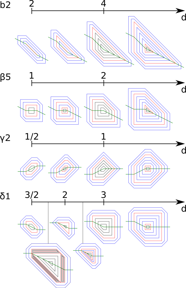
Figure 18: Bifurcation diagram for integer integrable polygon mappings with 3-piece force function and continuous $d\in\mathbb{R}$. Each row shows changes of phase space with shift parameter $d$. Phase space plots at exact values of $d$ correspond to bifurcations in a system and plots in between them show prototype of map for some value of $d$ in the corresponding interval of parameter.

VII 4-piece maps

In this section we will consider force function with four segments. Adding an extra segment results in total of 6 independent parameters defining the force function: 4 slopes $k_{1,2,3,4}$, shift parameter $d$ and ratio $r=l_{2}/l_{3}$. The scale transformation allows us to normalize one of two finite pieces ($l_{2}$ or $l_{3}$) to unity so only one of them is independent; alternatively we will use the ratio $r$ when it appears to be more convenient. In next three subsections we will present mappings isolated with respect to $d$ (finite set of integer values) and isolated with respect to $r$ as well, discrete $r$ (all positive integer values, $r\in\mathbb{N}^{+}$) or continuous $r$ (map is integrable for any $r\in\mathbb{R}^{+}$). Results of a search are summarized in Tables 5 and 6. In addition, more cases which were harder to classify are presented in the last Subsection VII.4.

		$r$			$r$
$[k_{1},k_{2},k_{3},k_{4}]$	1:1	1:2	1:3	1:3	1:2	1:1	$[k_{1},k_{2},k_{3},k_{4}]$
$[-1,-2,-1,-2]$		4,7					$[-2,-1,-2,-1]$
$[0,-2,0,-1]$	2	0	2			4	$[-1,0,-2,0]$
$[0,-1,1,-1]$	2			4		2	$[-1,1,-1,0]$
$[1,-2,0,-1]$		0					$[-1,0,-2,1]$
$[1,-1,0,-1]$	1		1			4	$[-1,0,-1,1]$
$[1,0,1,-1]$	1,2			4		2,1	$[-1,1,0,1]$
$[1,0,2,0]$					0		$[0,2,0,1]$
$[1,2,0,1]$		0					$[1,0,2,1]$

Table 5: Integrable polygon mappings with 4-piece force function and isolated integer $d$ and $r$. Such mappings were found only for $r=1,2,3$ and corresponding values of parameter $d$ (in units of $l_{2}$) are presented for each quadruplet of integer slopes.

$[k_{1},k_{2},k_{3},k_{4}]$	$d$	$r$	$r$	$d$	$[k_{1},k_{2},k_{3},k_{4}]$
$[0,-1,-2,-1]$	0	1	$\mathbb{N}^{+}$	$4+3/r$	$[-1,-2,-1,0]$
	1	$\mathbb{R}^{+}$	$\mathbb{R}^{+}$	$4+2/r$
$[0,-2,-1,0]$	0	$\mathbb{R}^{+}$	$\mathbb{R}^{+}$	$3+4/r$	$[0,-1,-2,0]$
	$2+1/r$	$\mathbb{R}^{+}$	$\mathbb{R}^{+}$	$2+2/r$
	$4+2/r$	$\mathbb{R}^{+}$	$\mathbb{R}^{+}$	1
$[0,-1,1,0]$	2	$\mathbb{R}^{+}$	$\mathbb{R}^{+}$	$1+1/r$	$[0,1,-1,0]$
$[0,1,2,0]$	1	$\mathbb{R}^{+}$	$\mathbb{R}^{+}$	0	$[0,2,1,0]$
$[1,-1,-2,-1]$	0	1	$\mathbb{N}^{+}$	$4+3/r$	$[-1,-2,-1,1]$
$[1,-1,0,-1]$	0	1	$\mathbb{N}^{+}$	$2+3/r$	$[-1,0,-1,1]$
$[1,0,-2,-1]$			$2,4,6,\ldots$	$4+3/(2r)$	$[-1,-2,0,1]$
$[1,-2,-1,0]$	0	$\mathbb{R}^{+}$	$\mathbb{R}^{+}$	$3+4/r$	$[0,-1,-2,1]$
$[1,0,-1,0]$	0	$\mathbb{R}^{+}$	$\mathbb{R}^{+}$	$3+2/r$	$[0,-1,0,1]$
	1	$\mathbb{R}^{+}$	$\mathbb{R}^{+}$	$3+1/r$
	$1+1/r$	$\mathbb{R}^{+}$	$\mathbb{R}^{+}$	$2+1/r$
$[1,2,1,0]$	0	$\mathbb{R}^{+}$	$\mathbb{R}^{+}$	1	$[0,1,2,1]$
	$1/r$	$\mathbb{N}^{+}$	1	0

Table 6: Integrable polygon mappings with 4-piece force function and isolated integer $d$ and discrete of continuous $r$. Values of parameters $d$ (in units of $l_{2}$) and $r$ are presented for each quadruplet of integer slopes.

VII.1 Isolated d and r

4-piece mappings with isolated integer values of $d$ and $r$ are shown in Fig. 19 and action angle variables are provided in Tables 8 and 9; these and all further tables with dynamical properties of 4-piece maps are moved to Appendix C for the reader’s convenience.

Naively we expected that layers of phase space change along with the force function and separatrices of motion are associated with vertices of $f(q)$, for example look at mappings b1.1, $\alpha$3.1, $\alpha$3.3 or $\beta$4.1. But results of our search are showing that dynamics can be more complicated. As one can see for mappings a1.1, a3.2, c1.1 and few others, an additional layer can appear on outer pieces of force function. This is due to the fact that polygons in one of them have sides decreasing with the amplitude; as a result, at some critical amplitude length of the side becomes equal to zero and invariant level sets transition to new layer. We would like to name this phenomena as long-range catastrophe.

Figure 19: Integer integrable polygon mappings with 4-piece force function and isolated values of shift parameter, $d$, and ratio of finite pieces, $r$.

VII.2 Isolated d, discrete r

In this subsection we present systems integrable with any positive integer ratio of $r=l_{1}/l_{2}\in\mathbb{N}^{+}$ but isolated integer values of the shift parameter $d$. Five different families of mappings with 2 prototypes from each are shown in Fig. 20. These maps are similar to 3-piece force function mappings with discrete $d$ (D) (Subsection VI.2): they all have chains of linear islands separating outer layers with nonlinear motion, and, the number of chains within the linear island is linearly growing with $r$. Rotation number $\nu_{i}$ for different layers are listed in Tables 10 and 11.

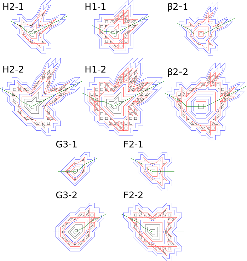
Figure 20: Integer integrable polygon mappings with 4-piece force function and isolated value of the shift parameter, $d$, and integer ratio of finite pieces $r\in\mathbb{N}^{+}$ (for the map $\beta$2-1 $r\in 2\mathbb{N}^{+}=2,4,6,\ldots$). For each family of mappings two first prototypes are presented.

VII.3 Isolated d, continuous r

Here we report systems which are integrable with any positive real ratio of $r=l_{1}/l_{2}\in\mathbb{R}^{+}$ but still isolated integer values of the shift parameter $d$. Some of them experience bifurcations of phase space with the change of parameter $r$ (mappings with ^′ index) while the rest of systems have same set of layers for any value of $r\in(0;\infty)$. Corresponding level sets of invariant and its bifurcation diagrams are shown below in Fig. 21. All dynamical properties are listed in Tables 12 and 13. Mapping $\alpha 3.1^{\prime}$ presents an interesting example: when $r=1$ outer otherwise nonlinear layer becomes mode-locked

$$\nu_{2}=\frac{1+r+y}{3+5\,r+4\,y}=\frac{2+y}{4(2+y)}=\frac{1}{4}.$$

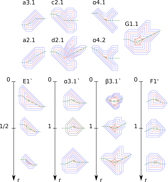
Figure 21: Integer integrable polygon mappings with 4-piece force function and isolated values of shift parameter, $d$, and continuous ratio of finite pieces, $r\in\mathbb{R}^{+}$. Mappings with ^′ index experience bifurcations of phase space with the change of parameter $r$.

VII.4 Additional cases

VII.4.1 Continuous and semi-continuous d with unity r.

When $r=1$, we found 2 dynamical systems which are integrable for any $d\in\mathbb{R}$: $\{0,-1,0,-1\}$ and $\{1,0,1,0\}$. In addition, map with slopes $\{-2,-1,-2,-1\}$ is integrable for any $d\geq 4$ (and its twin map $\{-1,-2,-1,-2\}$ is integrable for any $d\leq 3$).

VII.4.2 Non-unity values of r.

For values of $r$ different from 1, the situation is getting more complicated and more families of mappings appear. For example, for previously semi-continuous map $\{-2,-1,-2,-1\}$, we have at least four families with different behaviours of $d$:

$$\begin{array}[]{ll}d=4\,L_{2}+1&\quad(L_{2}\geq 1),\\ d=4\,L_{2}+2&\quad(L_{2}=1,2,3,\ldots),\\ d=4\,L_{2}+3&\quad(L_{2}=1,3,4,6,7,9,10,\ldots),\\ d=5\,L_{2}&\quad(L_{2}\geq 1);\end{array}$$

we say at least because our algorithm was limited to the range of $r=[1,2,...,9,10]$ and we can not guarantee the absence of integrable mappings out of this range.

For the continuous mappings we have

$$\begin{array}[]{llll}\{0,-1,0,-1\}:&&\{-1,0,-1,0\}:&\\[7.11317pt] d=L_{2}&\quad(L_{2}\geq 0),&d=2\,L_{2}&\quad(L_{2}\geq 0),\\ d=L_{2}+1&\quad(L_{2}\geq 0),&d=2\,L_{2}+1&\quad(L_{2}\geq 0),\\ d=2\,L_{2}+1&\quad(L_{2}\geq 0),&d=3\,L_{2}+1&\quad(L_{2}\geq 0),\\ d=2\,L_{2}+2&\quad(L_{2}=1,2,3,\ldots),&d=3\,L_{2}+2&\quad(L_{2}=1,2,3,\ldots),\\ d=2\,L_{2}+3&\quad(L_{2}=1,3,4,6,7,9,10,\ldots),&d=3\,L_{2}+3&\quad(L_{2}=1,3,4,6,7,9,10,\ldots),\\ d=3\,L_{2}&\quad(L_{2}\geq 1/2),&d=4\,L_{2}&\quad(L_{2}\geq 1/2),\end{array}$$

and

$$\begin{array}[]{llll}\{1,0,1,0\}:&&\{0,1,0,1\}:&\\[7.11317pt] d=0&\quad(L_{2}\geq 0),&d=L_{2}&\quad(L_{2}\geq 0),\\ d=1&\quad(L_{2}\geq 0),&d=L_{2}+1&\quad(L_{2}\geq 0),\\ d=L_{2}+1&\quad(L_{2}\geq 0),&d=2\,L_{2}+1&\quad(L_{2}\geq 0),\\ d=L_{2}+2&\quad(L_{2}=1,2,3,\ldots),&d=2\,L_{2}+2&\quad(L_{2}=1,2,3,\ldots),\\ d=L_{2}+3&\quad(L_{2}=1,3,4,6,7,9,10,\ldots),&d=2\,L_{2}+3&\quad(L_{2}=1,3,4,6,7,9,10,\ldots),\\ d=2\,L_{2}&\quad(L_{2}=1/2\quad\mathrm{and}\quad L2\geq 1),&d=3\,L_{2}&\quad(L_{2}=1/2,3/2\quad\mathrm{and}\quad L2\geq 2).\\ d=2&\quad(L_{1}:L_{2}=1:4),&&\end{array}$$

Finally, we have two more dynamical systems with complicated dependence of $d$ and $r$:

$$\begin{array}[]{llll}\{0,-1,0,1\}:&&\{1,2,1,0\}:&\\[7.11317pt] d=L2+2&\quad(L_{2}\geq 0),&d=1&\quad(L_{2}=3,4,5,\ldots),\\ d=L2+3&\quad(L_{2}\geq 0),&d=(L_{2}/2)+1&\quad(L_{2}=2,6,10,14,\ldots).\\ d=2\,L_{2}+1&\quad(L_{2}=1,2,4,5,7,8,10,\ldots),&&\\ d=2\,L_{2}+2&\quad(L_{2}=1,2,3,\ldots),&&\\ d=2\,L_{2}+3&\quad(L_{2}\geq 0),&&\\ d=(3/2)\,L_{2}+7/2&\quad(L_{2}=1,3,5,7,\ldots),&&\\ d=(3/2)\,L_{2}+3&\quad(L_{2}=2,4,6,8,\ldots),&&\\ d=(5/3)\,L_{2}+10/3&\quad(L_{2}=1,4,7,10,\ldots),&&\end{array}$$

Since there are too many mappings in this subsection, we did not provide any figures or tables with dynamical properties, leaving them as an exercise for the reader.

VIII Applications of mappings with polygon invariants

In the next three subsections we will discuss the importance and some practical applications of mappings with polygon invariants as well as its connection to other dynamical systems.

VIII.1 Connection to Painlevé equations and Suris mappings

Some integrable mappings with polygon invariants have a direct connection to discrete Painlevé equations (dP). Painlevé equations are nonlinear difference equations with canonical form being Levi et al. (1996); Grammaticos and Ramani (2004):

$$\begin{array}[]{lll}\mathrm{dP}_{\mathrm{I}}:&\displaystyle\quad X_{n+1}\,X_{n-1}=\frac{\lambda^{n}X_{n}+1}{X_{n}^{\sigma}},&\sigma=0,1,2,\\[9.95863pt] \mathrm{dP}_{\mathrm{II}}:&\displaystyle\quad X_{n+1}\,X_{n-1}=\frac{\alpha(\lambda^{n}+X_{n})}{X_{n}^{\rho}(1+\lambda^{n}X_{n})},&\rho=0,1,\\[9.95863pt] \mathrm{dP}_{\mathrm{III}}:&\displaystyle\quad X_{n+1}\,X_{n-1}=\frac{(X_{n}+\alpha\,\lambda^{n})(X_{n}+\alpha^{-1}\lambda^{n})}{(1+\beta\,\lambda^{n}X_{n})(1+\beta^{-1}\lambda^{n}X_{n})}.\end{array}$$ (6)

We will be interested in the autonomous (i.e. mappings do not have explicit dependence on $n$) limit of dP_I-III corresponding to $\lambda\to 1$. It is worth mentioning that autonomous limit of Eqs. (6) could be written in the Suris form by introducing a new set of variables $X_{n}=e^{x_{n}/\epsilon}$, $\alpha=e^{A/\epsilon}$, $\beta=e^{B/\epsilon}$:

$$\begin{array}[]{ll}\mathrm{dP}_{\mathrm{I}}^{\mathrm{S}}:&\displaystyle\quad x_{n+1}+x_{n-1}=\epsilon\,\log{\left[\frac{e^{x_{n}/\epsilon}+1}{e^{\sigma\,x_{n}/\epsilon}}\right]},\\[12.0925pt] \mathrm{dP}_{\mathrm{II}}^{\mathrm{S}}:&\displaystyle\quad x_{n+1}+x_{n-1}=A-\rho\,x_{n},\\[9.24706pt] \mathrm{dP}_{\mathrm{III}}^{\mathrm{S}}:&\displaystyle\quad x_{n+1}+x_{n-1}=\epsilon\,\log{\left[\frac{(e^{x_{n}/\epsilon}+e^{A/\epsilon})(e^{x_{n}/\epsilon}+e^{-A/\epsilon})}{(e^{x_{n}/\epsilon}+e^{B/\epsilon})(e^{x_{n}/\epsilon}+e^{-B/\epsilon})}\right]}.\end{array}$$ (7)

While the force function for dP${}_{\mathrm{II}}^{\mathrm{S}}$ is simply a linear function, two other cases are specific examples of integrable exponential Suris mapping.

The ultradiscretized form of Painlevé equations (udP) could be obtained by taking the limit $\epsilon\to 0$ in Eqs. (7). At this point we should clarify the terminology: by saying “discrete” Painlevé equation we refer to the difference nature of the equation in contrast to nonlinear second-order ordinary differential Painlevé equations. The addition “ultra” refers to another level of discretization when the force function is transitioning from a smooth continuous to a piecewise linear function. Using identity $\displaystyle\lim_{\epsilon\to 0}\epsilon\log{\left[\exp{(x/\epsilon)}+\exp{(y/\epsilon)}\right]}=\max(x,y)$ we arrive to

$$\begin{array}[]{ll}\mathrm{udP}_{\mathrm{I}}:&\displaystyle\quad x_{n+1}+x_{n-1}=\max{(x_{n},0)}-\sigma\,x_{n},\\[7.11317pt] \mathrm{udP}_{\mathrm{II}}:&\displaystyle\quad x_{n+1}+x_{n-1}=A-\rho\,x_{n},\\[7.11317pt] \mathrm{udP}_{\mathrm{III}}:&\displaystyle\quad x_{n+1}+x_{n-1}=\max{(x_{n},A)}+\max{(x_{n},-A)}-\max{(x_{n},B)}-\max{(x_{n},-B)}.\end{array}$$ (8)

The udP equations (8) have a symplectic Suris form $x_{n+1}+x_{n-1}=f(x_{n})$ with following ultradiscrete piecewise linear force functions

$$\begin{array}[]{l}\displaystyle f_{\mathrm{I}}(x)\,\,=\frac{1}{2}\left(|x|+x\right)-\sigma\,x=\begin{cases}(1-\sigma)\,x,&\textrm{for }x\geq 0,\\ -\sigma\,x,&\textrm{for }x<0,\end{cases}\\[14.22636pt] \displaystyle f_{\mathrm{II}}(x)\,\,\!=A-\rho\,x,\\[2.84544pt] \displaystyle f_{\mathrm{III}}(x)=\frac{1}{2}\left(|x+A|+|x-A|-|x+B|-|x-B|\right)=\begin{cases}0,&\textrm{for }x\in[B,\infty),\\ x-B,&\textrm{for }x\in[A,B),\\ A-B,&\textrm{for }x\in[-A,A),\\ -B-x,&\textrm{for }x\in[-B,-A),\\ 0,&\textrm{for }x\in(-\infty,-B).\end{cases}\end{array}$$ (9)

The force function $f_{\mathrm{I}}$ (corresponding to the first equation udP_I) is the simplest two-piece linear force without shift parameter, $d=0$, and with slopes defined as $(k_{1},k_{2})=(-\sigma,1-\sigma)$. Since $\sigma$ can only take values 0,1 and 2, we obtain previously considered mappings G, F and E respectively (see Fig. 10). The second ultradiscretized Painlevé equation has a trivial linear force function $f_{\mathrm{II}}$ and is integrable for any values of parameters $A$ and $\sigma$. In the case of integer slopes this results in 3 mappings with stable trajectories Cairns et al. (2014) $\alpha$, $\beta$, $\gamma$ and 2 unstable mappings $a$, $b$ (see Fig. 10). Finally, for the third ultradiscretized Painlevé equation udP_III (assuming $B>A>0$), we obtain force function containing five pieces. Taking the limit $A=\mathrm{const}$ and $B\to\infty$, from Eq. (9) we have the linear map $\alpha$ with slope of force function $k_{1}=-1$. Considering another limiting case $A\to 0$, one can see that $f(x)$ could be reduced to one of our 4-piece polygon maps $\alpha 3.1^{\prime}$ (slope coefficients $\{k_{1},k_{2},k_{3},k_{4}\}=\{0,-1,1,0\}$ and $d=2B$) with ratio parameter restricted to $r=1$ (note that our map $\alpha 3.1^{\prime}$ is integrable for arbitrary $r$, see Fig. 21). Figure 22 shows invariant level sets for this last case for different values of $\epsilon$. As one can see, approaching the ultradiscrete level $\epsilon\to 0$, the force function transitions to piecewise linear and level sets transform to polygons. When $\epsilon=\infty$ map becomes linear with $\nu=1/4$; note that invariant level sets are chosen as circles and not polygons. As we previously discussed linear mappings with rational rotation numbers are degenerate and allow infinitely many invariants of motion, but in this case the shape is chosen as a limiting case $\epsilon\to\infty$ for the exponential Suris invariant.

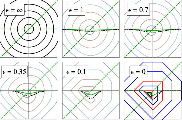
Figure 22: Constant level sets of invariant on $(x_{n},x_{n+1})$ plane for discrete Painlevé map dP${}_{\mathrm{III}}^{\mathrm{S}}$ in Suris form with $A=0$ and $x$ measured in units of $B$. For $\epsilon=\infty$ map degenerate to linear with $f(x)=0$ and level sets degenerate to concentric circles. When $\epsilon=0$ we observe ultradiscrete limit udP_III corresponding to polygon map $\alpha 3.1^{\prime}$ with ratio of finite pieces restricted to unity, $r=1$. Black and blue level sets show trajectories in linear and nonlinear areas of phase space, red level sets are separatrices of motion between different layers. Green curve is the second symmetry line $f(x)/2$ and black dashed curve is the force function $f(x)$.

We would like to emphasize that our polygon mappings represent a much richer family of integrable systems beyond ultradiscretezations of known Painlevé equations udP${}_{\mathrm{I\text{--}III}}$; ultradiscretized equations of Painlevé type are limited to only 5-piece force functions and the set of parameters is very restricted (e.g. slopes of outer pieces of 5-piece force functions can only be equal to zero).

VIII.2 Near-integrable systems

Since force function is piecewise linear and isn’t smooth (not differentiable at discrete set of points), it might seems that these polygon mappings are somewhat impractical. However, in a similar manner to the example in Fig. 22 where the polygon mapping can be smoothed using parameter $\epsilon$, below we will demonstrate how one can construct not integrable, but quasi-integrable systems. One of the possible ways to perform this was first done by Cohen Moser (1993); Rychlik and Torgerson (1998) in application to Brown-Knuth map (map H) by introducing a new force function as

$$f(q)=\sqrt{q^{2}+\epsilon^{2}}\underset{\epsilon\to 0}{\to}|q|.$$

As one can see it tends to $|q|$ as $\epsilon\to 0$ or at large amplitudes as $q\to\infty$. Fig. 23 shows a comparison between Cohen and Brown-Knuth maps. Looking at the tracking results one can see that new $f(q)$ produces a system with surprisingly regular behavior. However, detailed numerical experiments reveal multiple island structures at small scales (see Fig. 23 case (c.)) indicating that analytic invariant doesn’t exist.

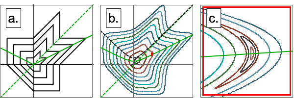
Figure 23: The left plot (a.) illustrates invariant level sets for the Brown-Knuth map, force function $f(q)=|q|$. The middle plot (b.) displays invariant level sets for the Cohen map, $f(q)=\sqrt{q^{2}+1}$. The right plot (c.) again provides invariant level sets for the Cohen map, but on a different scale showing one of the island structures. The level sets for Cohen map are obtained by tracking. The green curve is the second symmetry line $p=f(q)/2$.

Thus, in a similar manner, one can first rewrite a general $n$-piece linear function using one linear and $(n-1)$ modulus functions in a form $k_{i}|q-q_{i}|$ where $q_{i}$ is a location of $i-th$ vertex, then substitute all modulus with square roots $k_{i}|q-q_{i}|\to k_{i}\sqrt{(q-q_{i})^{2}+\epsilon^{2}}$, resulting in

$$\begin{array}[]{lll}\displaystyle n=2:&\displaystyle\quad\frac{k_{1}+k_{2}}{2}\,q+\frac{k_{2}-k_{1}}{2}\,\sqrt{q^{2}+\epsilon^{2}}+d&\displaystyle\underset{\epsilon\to 0}{\to}\,\,d+q\times\left\{\begin{array}[]{cc}k_{1},&q<0,\\ k_{2},&q\geq 0,\end{array}\right.\\[9.95863pt] \displaystyle n=3:&\displaystyle\quad\frac{k_{1}+k_{3}}{2}\,q+\frac{k_{2}-k_{1}}{2}\,\sqrt{q^{2}+\epsilon^{2}}+\frac{k_{3}-k_{2}}{2}\,\sqrt{(q-1)^{2}+\epsilon^{2}}-\frac{k_{3}-k_{2}}{2}+d&\displaystyle\underset{\epsilon\to 0}{\to}\,\,d+q\times\left\{\begin{array}[]{cl}k_{1},&q<0,\\ k_{2},&0\leq q<1,\\ k_{3},&q\geq 1,\end{array}\right.\\[7.11317pt] \ldots&\qquad\displaystyle\ldots.\end{array}$$

Fig. 24 below shows examples of how the “smoothening” procedure can be used to produce new nearly integrable systems. More importantly, in addition to being near integrable, these mappings are stable since limiting polygon at larger amplitudes provides an isolating integral.

Note that from a practical standpoint, the fact that produced systems are quasi- and not exactly integrable is not a problem as long as $\epsilon$ is sufficiently small and chaotic formations are within needed tolerances. Even if a system is originally designed as integrable, small errors (e.g. rounding errors for simulations, or tolerance errors for physical experimental setups) will destroy integrability on a small scale. Also, the square root function is only one of infinitely many ways of smoothing force function (e.g. one can use $\arctan$, $\tanh$ or others) and is used here as an example.

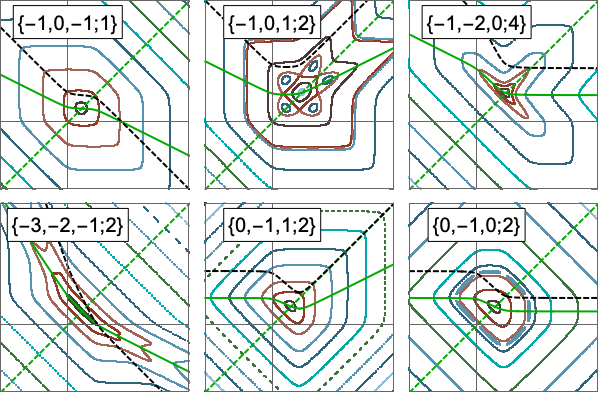
Figure 24: Examples of quasi-integrable systems produced by “smoothening” 3-piece integrable polygon maps using $\epsilon=0.05$. For each plot the label shows parameters $\{k_{1},k_{2},k_{3};d\}$. All level sets are obtained by tracking. The green curve is the second symmetry line $f(q)/2$ and the black dashed curve is the force function $f(q)$.

VIII.3 Discrete perturbation theory

Finally, knowledge of all possible integrable mappings with polygon invariants will not only help to construct new near integrable systems, but to understand dynamics and phase space of more general non-integrable mappings with smooth $f(p)$. This can be done by discretizing $f(p)$ by a piecewise linear function; so we have a perturbation theory where order is determined by number of pieces and smallness parameter is defined by a smallest piece of force function. In order to demonstrate the idea, we provide a comparison of a phase space for chaotic quadratic

$$f(p)=a\,q+q^{2}$$

and cubic Hénon maps

$$f(p)=a\,p+q^{3}$$

around specific resonances ($\nu=1/4$ and stop band $\nu=1/2$) and corresponding polygon maps. As one can see in Fig. 25 below, even low order approximations can reveal important qualitative dynamical features, including shapes of trajectories in phase space and the topological structure of the phase portrait.

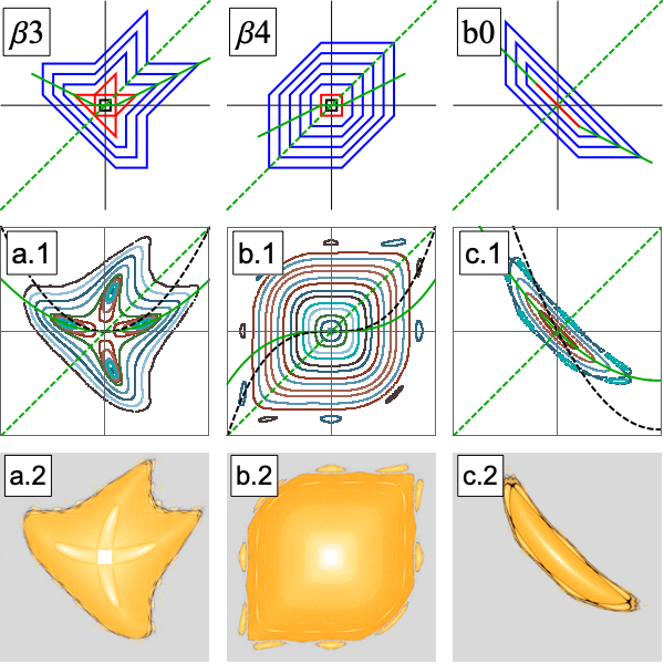
Figure 25: The middle row of plots (a.1 – c.1) shows tracking for Hénon map with quadratic $f(q)=a\,q+q^{2}$ (cases a. and c.), and cubic force functions $f(q)=a\,q+q^{3}$ (case b.). The value of parameter is (a.) $a=a_{1/4}-0.005$, (b.) $a=a_{1/4}+0.005$ and (c.) $a=a_{1/2}+0.05$, where $a_{1/4}=0$ is the main octupole resonance with $\nu=1/4$ and $a_{1/2}=-2$ is the linear-half integer stopband $\nu=1/2$. The green curve is the second symmetry line $f(q)/2$ and the black dashed curve is the force function $f(q)$. All plots correspond to a range $p,q\in[-1,1]$. The top row shows corresponding low order approximation via mappings with polygon invariants. The bottom row of plots (a.2 – c.2) shows $\log$ of SALI values for the same cases, by courtesy of Ivan Morozov (BINP).

An interesting observation can be made looking at the smaller alignment index (SALI) color maps. SALI is an indicator (alternative to traditional maximal Lyapunov exponent) distinguishing between ordered and chaotic motion Skokos et al. (2003). As one can see, there is a significant area around a fixed point with almost the same color (white). It means that in this area the motion is quasi-integrable and almost linear (very small variation of rotation number). One can note that this area resembles a separatrix of inner linear layer from corresponding polygon map; thus, we learn that linear dynamics in the inner layer of integrable polygon map is not just a consequence of oversimplified discretization of force function, but a reflection of actual dynamics — negligible spread of rotation numbers. In contrast to smooth perturbation theory when in zeroth order we have an ellipse $\mathcal{K}(p,q)=p^{2}-a\,p\,q+q^{2}$, here we have a polygon with degenerate motion. While in both approaches the rotation number is independent of amplitude, discrete perturbation theory gives better boundary of linear area when system is close to some resonant condition, while smooth perturbation theory will work better far away from any major resonances or very close to the origin where ellipses are not distorted.

IX Summary

In this article, we presented an algorithm for automated discovery of new integrable symplectic maps of the plane with polygon invariants, and as a result, we reported over 100 new integrable families. The algorithm successfully rediscovered some famous discrete Painlevé equations as well as some of McMillan-Suris integrable mappings. Fig. 26 presents most, but not all, systems discovered by the search algorithm. They are grouped by similarity of dynamics around the fixed point while arrows are pointed toward systems with more segments in $f$, thus showing hierarchy.

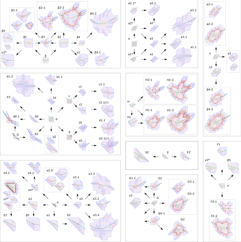
Figure 26: Most (but not all) mappings discovered by an algorithm: 1- through 4-piece force functions. Maps are organized by dynamics around fixed point; systems with the same rotation number around fixed points are presented in the same solid box. Dashed boxes indicates that map belongs to discrete or continuous family.

While the discovered systems have a piecewise linear force and polygon invariants, thus lacking the differentiability, we suggested a “smoothening” procedure which can produce new quasi-integrable systems without singularities. Such “smooth” polygon maps have potential applications in physics, engineering, dynamical system theory, and signal processing. For example, in accelerator physics, such near-integrable systems could reduce unwanted particle losses in accelerators and, thus, improve their performance and the achievable beam intensities. So far, the design of integrable accelerator focusing systems is at its very beginning, even conceptually. Fermilab presently operates the first accelerator Antipov et al. (2017), designed to test some of these concepts.

Finally, we introduced a discrete perturbation theory in order to relate our polygon mappings to a general symplectic map of a plane. The theory furthers understanding of shapes of phase space curves and approximates dynamics for more realistic chaotic systems such as Hénon or Chirikov mappings or even integrable ones, such as McMillan-Suris maps.

It remains an open question whether one can understand the totality of all maps with polygon invariants, and not only corresponding to force functions with integers coefficients. For example, it is not clear whether there exists some sort of generating formula allowing to derive integrable maps with $n+1$ piece force function from mappings with $n$-pieces.

X Acknowledgments

The authors would like to thank Eric Stern (FNAL) and Taylor Nchako (Northwestern University) for carefully reading this manuscript and for their helpful comments. Moreover, we would like to extend our gratitude to Ivan Morozov (BINP) for multiple discussions and his generous contributions in preparation of Subsection VIII.3 and especially Fig. 25. Finally we would like to express our deep appreciation for Nikolay Kuropatkin’s (FNAL) useful discussion on vertex count of polygons.

Y. K. acknowledges funding by the DoE ASCR Accelerated Research in Quantum Computing program (award No. DE-SC0020312), DoE QSA, NSF QLCI (award No. OMA-2120757), NSF PFCQC program, DoE ASCR Quantum Testbed Pathfinder program (award No. DE-SC0019040), U.S. Department of Energy Award No. DE-SC0019449, AFOSR, ARO MURI, AFOSR MURI, and DARPA SAVaNT ADVENT.

This manuscript has been authored by Fermi Research Alliance, LLC under Contract No. DE-AC02-07CH11359 with the U.S. Department of Energy, Office of Science, Office of High Energy Physics.

Appendix A Calculation of action-angle variables for polygon mappings

A.1 Action

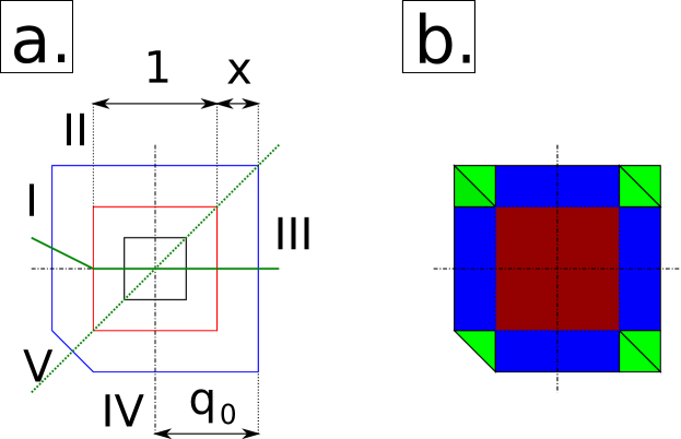
Figure 27: Calculation of action-angle variables for map $\beta$1. Plot (a.) shows three level sets of invariant: level set from linear layer (black), separatrix (red) and level set from nonlinear layer (blue). Solid and dotted green lines are second ($p=f(q)/2$) and first ($p=q$) symmetry lines. Segments of nonlinear trajectory are labeled with Roman numerals. Plot (b.) shows partition of the area under nonlinear trajectory into fundamental rectangles and triangles. Area of green triangles is proportional to initial condition squared, area of blue rectangles is linearly proportional and red square is independent of $q_{0}$.

Since invariant curves are polygons, the calculation of the area enclosed under the trajectory is a trivial task. Each polygon can be split into collection of simple rectangles and (or) triangles. Thus, the action integral (as well as partial action integral) has the form

$$\begin{array}[]{l}\displaystyle J=\frac{1}{2\,\pi}\,\oint p\,\mathrm{d}q=C_{1}q_{0}^{2}+C_{2}q_{0}+C_{3},\\[8.5359pt] \displaystyle J^{\prime}=\frac{1}{2\,\pi}\,\int_{q_{0}}^{q^{\prime}_{0}}p\,\mathrm{d}q=C^{\prime}_{1}q_{0}^{2}+C^{\prime}_{2}q_{0}+C^{\prime}_{3}\end{array}$$ (10)

where $C^{(^{\prime})}_{1,2,3}$ are some constants and $(q_{0},0)$ is an initial condition on the trajectory. The first term represents rectangles (or triangles) with both sides being proportional to initial conditions, the next term with only one side of rectangle being proportional to $q_{0}$ and the other side determined by map parameters, and the final term represents contribution from fundamental rectangles independent of initial condition.

As an example, below we will calculate action and partial action for the outer layer of nonlinear trajectories of the map $\beta 1$, see Fig. 27. Introducing a new variable $x=|q_{0}-1/2|$ which represents a horizontal distance from separatrix to nonlinear trajectory, we have

$$\begin{array}[]{l}\displaystyle J=\frac{1}{2\,\pi}\,\left(\frac{7}{2}x^{2}+4x+1\right),\\[8.5359pt] \displaystyle J^{\prime}=\frac{1}{2\,\pi}\,\left(x^{2}+x+\frac{1}{4}\right).\end{array}$$ (11)

A.2 Rotation number and angle variable

The dynamics of map in action-angle variables is given by

$$\begin{array}[]{rl}J_{n}&\!\!=J_{0},\\[5.69046pt] \theta_{n}&\!\!=\theta_{0}+2\,\pi\,\nu\,n,\end{array}$$

where $\nu$ is rotation number and $\theta_{0}$ is an initial phase which can be defined, let’s say, as an initial polar angle on the trajectory measured around fixed point

$$\theta_{0}=\arctan\frac{p_{0}-p_{f}}{q_{0}-q_{f}}.$$

Below we provide 2 methods of calculation of $\nu$; both methods are based on Danilov theorem, see Zolkin et al. (2017); Nagaitsev and Zolkin (2020); Mitchell et al. (2021). In addition, along with the second method we will show how to verify the integrability of the map.

A.2.1 Method I

According to Danilov theorem, the rotation number is given as a derivative of the partial action (Hamiltonian) over the action variable. Using chain rule for derivatives and Eq. (10), we have

$$\nu=\frac{\mathrm{d}J^{\prime}}{\mathrm{d}J}=\frac{\mathrm{d}J^{\prime}/\mathrm{d}q_{0}}{\mathrm{d}J/\mathrm{d}q_{0}}=\frac{C^{\prime}_{2}+2\,C^{\prime}_{1}q_{0}}{C_{2}+2\,C_{1}q_{0}}.$$

As one can see, for all mappings, the dependence of rotation number on linear amplitude is always a rational function of a degree 1. In addition, one can conclude that for all rational (irrational) initial conditions $x\in\mathbb{Q}$ ($\in\mathbb{R}\setminus\mathbb{Q}$) the rotation number is rational (irrational) as well, so the trajectory is periodic (quasi-periodic).

Again using mapping $\beta 1$ as an example we have

$$\nu=\frac{4|q_{0}|}{1+14|q_{0}|}=\frac{1+2x}{4+7x},\qquad|q_{0}|>1/2.$$

As we expect, for $x=0$ we have $\nu=1/4$ matching rotation number on the separatrix and inner linear layer (limiting case for map $\beta$), and, for large amplitudes $\displaystyle\lim_{x\to\infty}\nu=2/7$ (limiting case map F).

A.2.2 Method II

Here we present another method which does not involve direct calculation of action and partial action. Instead, one can directly use Danilov formula

$$\nu=\frac{\displaystyle\oint\left(\frac{\partial\mathcal{K}}{\partial p}\right)^{-1}\,\mathrm{d}q}{\displaystyle\int_{q}^{q^{\prime}}\left(\frac{\partial\mathcal{K}}{\partial p}\right)^{-1}\,\mathrm{d}q}$$

where integrals are taken along the constant level set of invariant $\mathcal{K}(p,q)=\mathrm{const}$. Since level set is polygon, each integral can be seen as a sum of integrals along its sides. If polygon has vertical sides, corresponding integrals should be replaced with (see Zolkin et al. (2017); Nagaitsev and Zolkin (2020))

$$\int\left(\frac{\partial\mathcal{K}}{\partial p}\right)^{-1}\,\mathrm{d}q\qquad\rightarrow\qquad\int\left(-\frac{\partial\mathcal{K}}{\partial q}\right)^{-1}\,\mathrm{d}p.$$

Let’s use the already familiar mapping $\beta$1 as an example. First, we label sides of invariant polygon corresponding to nonlinear layer using Roman numerals (see Fig. 27). Then, we write down the equation for each side of polygon using $q_{0}:(0,q_{0})\in\mathcal{K}(p,q)=\mathrm{const}$ (see Table 7). In general one can use any point $(p_{0},q_{0})$ belonging to the invariant curve, and, $p_{0}=0$ is chosen due to a convenience without any loss of generality. Now we can use initial condition $q_{0}$ as an invariant of motion $\mathcal{K}(p,q)\equiv q_{0}$ and find it from the equation of the polygon segment (third column in table). Then, the integral in denominator can be calculated as

$$\oint\left(\frac{\partial\mathcal{K}}{\partial p}\right)^{-1}\,\mathrm{d}q=\underbrace{\int_{-1/2}^{1/2+x}1\,\mathrm{d}p}_{\mathrm{I}}+\underbrace{\int_{-1/2-x}^{1/2+x}1\,\mathrm{d}q}_{\mathrm{II}}+\underbrace{\int_{1/2+x}^{-1/2-x}(-1)\,\mathrm{d}p}_{\mathrm{III}}+\underbrace{\int_{1/2+x}^{-1/2}(-1)\,\mathrm{d}q}_{\mathrm{IV}}+\underbrace{\int_{-1/2}^{-1/2-x}(-1)\,\mathrm{d}q}_{\mathrm{V}}=4+7x.$$

Using initial condition $(q_{0},0)$, the integral in numerator is

$$\int_{(q_{0},0)}^{(0,p_{1})}\left(\frac{\partial\mathcal{K}}{\partial p}\right)^{-1}\,\mathrm{d}q=\underbrace{\int_{0}^{1/2+x}1\,\mathrm{d}p}_{\mathrm{I}}+\underbrace{\int_{-1/2-x}^{0}1\,\mathrm{d}q}_{\mathrm{II}}=1+2x.$$

One can see that the resulting rotation number is the same as in Method I:

$$\nu=\frac{1+2x}{4+7x}.$$

Finally, using explicit expressions for each side of the polygon we can verify an integrability of the map. For that we will check that both symmetries are satisfied. The first symmetry is that for the entire polygon we have:

$$\mathcal{K}(q,p)=\mathcal{K}(p,q).$$

It is easy to see that vertical side I (III) is the symmetric pair to side IV (II), while segment V is its own pair since its invariant under $q\leftrightarrow p$. The second symmetry is guaranteed by McMillan condition, i.e. vertically opposite sides are equidistant from the second symmetry line or alternatively the sum of opposite sides is equal to the force function:

$$\begin{array}[]{llll}\mathrm{II+IV}&\!\!\!:\quad q_{0}+(-q_{0})&\!\!=0&\!\!=f(q>-1/2),\\[7.11317pt] \mathrm{II+V}&\!\!\!:\quad q_{0}+(-q-q_{0}-1/2)&\!\!=-q-1/2&\!\!=f(q\leq-1/2).\end{array}$$

Additionally, vertical sides I and III are split in halves by symmetry line. Therefore we verify an integrability since both symmetries hold for any $q_{0}$. In a similar manner, all mappings presented in this article were confirmed to be integrable.

Side #	Equation	$\mathcal{K}(q,p)\equiv q_{0}$	$(\partial\mathcal{K}/\partial p)^{-1}$	$-(\partial\mathcal{K}/\partial q)^{-1}$
I:	$q=-q_{0}$	$-q$	—	1
II:	$p=q_{0}$	$p$	1	—
III:	$q=q_{0}$	$q$	—	-1
IV:	$p=-q_{0}$	$-p$	-1	—
V:	$p=-q-q_{0}-1/2$	$-p-q-1/2$	-1	1

Table 7: Equation of a side, expression for the invariant along with its partial derivatives for the polygon in outer nonlinear layer of the map $\beta 1$.

Appendix B Pseudo-code for the search algorithm

Input : $V^{\mathrm{cutoff}}\in\mathbb{Z}$ — cutoff parameter for polygon vertex count,

$q_{\mathrm{ini}}^{\mathrm{max}}\in\mathbb{Z}\,\,(\sum_{i=2}^{n}l_{i}<q_{\mathrm{ini}}^{\mathrm{max}}<r_{\mathrm{max}})$ — max initial condition.

Output : $integrable\in\mathbb{B}$ — integrability of map.

/* Map is integrable unless unstable or chaotic orbit is detected */

$integrable\leftarrow\mathrm{True}$

/* Scan over all initial conditions from fixed point $q^{*}$ to $q_{\mathrm{max}}$ */

for $q=q^{*},\ldots,q_{\mathrm{ini}}^{\mathrm{max}}$

{

    /* Compute number of vertexes for given orbit */

    $V\leftarrow vertex(q)$

    /* If motion is stable */

    if $V\neq-1$ then

       /* If the number of vertices in the orbit polygon is larger than a cutoff value, $V^{\mathrm{cutoff}}$ */

       if $V>V^{\mathrm{cutoff}}$ then

          /* Exclude map if any of orbits is chaotic */

          $\,\!integrable\leftarrow\mathrm{False}$

    /* Exclude map if any of orbits is unstable */

    else $integrable\leftarrow\mathrm{False}$

{

return $integrable$

Algorithm 1 Map analyzer. Algorithm verifies if a map is integrable with invariant level sets being polygons. Algorithm needs function $vertex(q)$ and force function.

Input : $n\equiv\mathrm{dim}\,\mathbf{k}\geq 2$ — number of segments,

$q\in\mathbb{R}$ — coordinate,

$\mathbf{k}=(k_{1},k_{2},\ldots,k_{n})\in\mathbb{Z}^{n}$ — vector of slopes of segments,

$\mathbf{l}\,\,\,\!=(l_{2},l_{3},\ldots,l_{n-1})\in\mathbb{R}^{n-2}$ — vector of finite segments’ length.

Output : $f(q,\mathbf{k},\mathbf{l})\in\mathbb{R}$ — value of force function.

/* Compute force function value depending on segment */

switch $q$

{

    /* 1-st segment */

    case $q\leq 0$

       $f\leftarrow k_{1}q$

    /* 2-nd segment */

    case $0<q\leq l_{2}$

       $f\leftarrow k_{2}q$

    /* 3-rd segment */

    case $l_{2}<q\leq l_{2}+l_{3}$

       $f\leftarrow k_{3}(q-l_{2})+k_{2}l_{2}$

    …

    /* $(n-1)$-th segment */

    case $\sum_{i=2}^{n-2}l_{i}<q\leq\sum_{i=2}^{n-1}l_{i}$

       $f\leftarrow k_{n-1}(q-\sum_{i=2}^{n-2}l_{i})+\sum_{i=2}^{n-2}k_{i}l_{i}$

    /* $n$-th segment */

    case $q>q\sum_{i=2}^{n-1}l_{i}$

       $f\leftarrow k_{n}(q-\sum_{i=2}^{n-1}l_{i})+\sum_{i=2}^{n-1}k_{i}l_{i}$

}

return $f$

Algorithm 2 Continuous piecewise linear force function $f(q,\mathbf{k},\mathbf{l})$ with first vertex at the origin.

$$f(l_{s-1}<q\leq l_{s},\mathbf{k},\mathbf{l})=k_{s}(q-\sum_{i=2}^{s-1}l_{i})+\sum_{i=2}^{s-1}k_{i}l_{i},\qquad\qquad l_{1}=0,\,l_{0,n}=\mp\infty.$$

Input :  $\!\!q_{\mathrm{ini}}\in\mathbb{R}$ — initial coordinate on a second symmetry line,

$\mathbf{k}=(k_{1},k_{2},\ldots,k_{n})\in\mathbb{Z}^{n}$ — vector of slopes of segments,

$\mathbf{l}\,\,\,\!=(l_{2},l_{3},\ldots,l_{n-1})\in\mathbb{R}^{n-2}$ — vector of finite segments’ length,

$d\in\mathbb{R}$ — force function shift parameter,

$N\in\mathbb{Z}$ — number of iterations,

$r_{\mathrm{max}}\in\mathbb{R}\,\,(\gg\sum_{i=2}^{n-1}l_{i})$ — max distance allowed in simulation,

$\eta\in\mathbb{R}\setminus\mathbb{Q}\,\,(\ll 1)$ — small irrational parameter to shift initial conditions,

$\epsilon\in\mathbb{R}\,\,(\ll 1)$ — collinearity cutoff parameter.

Output : $V$ — number of vertex of orbit ($V=-1$ if orbit is unstable).

$V\leftarrow 0$

/* Initial condition on 2-nd symmetry line with small irrational shift */

$q\leftarrow q_{\mathrm{ini}}+\eta$

$p\leftarrow[f(q,\mathbf{k},\mathbf{l})+d]/2$

/* Orbit, $\vec{\zeta}=(\zeta_{1},\zeta_{2},\ldots,\zeta_{N})$ */

for $i=1,\ldots,N$

{

    $\zeta_{i}\leftarrow(q,p)$

    $q^{\prime}\leftarrow p$

    $p^{\prime}\leftarrow-q+f(p)+d$

    $q\leftarrow q^{\prime}$

    $p\leftarrow p^{\prime}$

    /* Stop if radius of point in the phase space is $>r_{\mathrm{max}}$ */

    if $q^{2}+p^{2}>r_{\mathrm{max}}^{2}$ then

    {

       $V\leftarrow-1$

       break

    }

    else

    {

       /* Stop if orbit is periodic */

       if $q^{\prime}=q_{\mathrm{ini}}\land p^{\prime}=[f(q_{\mathrm{ini}},\mathbf{k},\mathbf{l})+d]/2$ then

          break

    }

}

/* Compute number of polygon vertexes, $V$, if the orbit is stable ($V\neq-1$) */

if $V\neq-1$ then

{

    Sort $\vec{\zeta}=(\zeta_{1},\ldots,\zeta_{N})$: $\forall\,0<k<N\quad\left[\arctan\frac{p_{k}}{q_{k}}>\arctan\frac{p_{k+1}}{q_{k+1}}\right]$

    Add $\zeta_{1}$ and $\zeta_{2}$ to the tail of $\vec{\zeta}$: $\vec{\zeta}\leftarrow(\zeta_{1},\zeta_{2},\ldots,\zeta_{N-1},\zeta_{N},\zeta_{1},\zeta_{2})$

    for $j=1,\ldots,N$

    {

       /* Compute dot product between displacement vectors */

       $\displaystyle\alpha_{j}=\frac{(p_{j+2}-p_{j+1})(p_{j+1}-p_{j})+(q_{j+2}-q_{j+1})(q_{j+1}-q_{j})}{\sqrt{(p_{j+2}-p_{j+1})^{2}+(q_{j+2}-q_{j+1})^{2}}\sqrt{(p_{j+1}-p_{j})^{2}+(q_{j+1}-q_{j})^{2}}}$

       /* New polygon vertex detection */

       if $||\alpha_{j}|-1|>\epsilon$ then

          V++

    }

}

return $V$

Algorithm 3 Function $vertex(q)$. Algorithm counts number of vertexes $V$ for a given orbit with initial condition on 2-nd symmetry line $(q,p)=(q_{\mathrm{ini}},f(q_{\mathrm{ini}})/2)$ or returns value of $(-1)$ if trajectory is unstable.

Appendix C Action-angle variables for 4-piece mappings

In Tables 8–13 below we provide rotation number $\nu$, action $J$ and partial action $J^{\prime}$ for integer integrable mappings with 4-piece force function.

Map	$\nu_{1},\,J_{1},\,J^{\prime}_{1}$	$\nu_{2},\,J_{2},\,J^{\prime}_{2}$	$\nu_{3},\,J_{3},\,J^{\prime}_{3}$
$\alpha$3.1	$\frac{1+x}{3+5x},\,x\in[0;1]$	$\frac{2+2y}{8+7y},\,y\in[0;\infty]$
	$\frac{5}{2}x^{2}+3x+\frac{1}{2}$	$\frac{7}{2}y^{2}+8y+J_{1}(1)$
	$\frac{1}{2}x^{2}+x+\frac{1}{6}$	$y^{2}+2y+J^{\prime}_{1}(1)$
$\alpha$3.2	$\frac{3+x}{9+5x},\,x\in[0;1]$	$\frac{4+3y}{14+10y},\,y\in[0;2]$	$\frac{10+2z}{34+7z},\,z\in[0;\infty]$
	$\frac{5}{2}x^{2}+9x+\frac{9}{2}$	$5y^{2}+14y+J_{1}(1)$	$\frac{7}{2}z^{2}+34z+J_{2}(2)$
	$\frac{1}{2}x^{2}+3x+\frac{3}{2}$	$\frac{3}{2}y^{2}+4y+J^{\prime}_{1}(1)$	$z^{2}+10z+J^{\prime}_{2}(2)$
$\alpha$3.3	$\frac{1+x}{3+5x},\,x\in[0;1]$	$\frac{2+2y}{8+9y},\,y\in[0;\infty]$
	$\frac{5}{2}x^{2}+3x+\frac{1}{2}$	$\frac{9}{2}y^{2}+8y+J_{1}(1)$
	$\frac{1}{2}x^{2}+x+\frac{1}{6}$	$y^{2}+2y+J^{\prime}_{1}(1)$
$\alpha$3.4	$\frac{1+x}{3+5x},\,x\in[0;3]$	$\frac{4+3y}{18+14y},\,y\in[0;2]$	$\frac{10+2z}{46+9z},\,z\in[0;\infty]$
	$\frac{5}{2}x^{2}+3x+\frac{1}{2}$	$7y^{2}+18y+J_{1}(3)$	$\frac{9}{2}z^{2}+46z+J_{2}(2)$
	$\frac{1}{2}x^{2}+x+\frac{1}{6}$	$\frac{3}{2}y^{2}+4y+J^{\prime}_{1}(3)$	$z^{2}+10z+J^{\prime}_{2}(2)$
$\beta$4.1	$\frac{1+x}{4+6x},\,x\in[0;1]$	$\frac{2+2y}{10+9y},\,y\in[0;\infty]$
	$3x^{2}+4x+1$	$\frac{9}{2}y^{2}+10y+J_{1}(1)$
	$\frac{1}{2}x^{2}+x+\frac{1}{4}$	$y^{2}+2y+J^{\prime}_{1}(1)$
$\beta$4.2	$\frac{3+x}{12+6x},\,x\in[0;1]$	$\frac{4+3y}{18+13y},\,y\in[0;2]$	$\frac{10+2z}{44+9z},\,z\in[0;\infty]$
	$3x^{2}+12x+9$	$\frac{13}{2}y^{2}+18y+J_{1}(1)$	$\frac{9}{2}z^{2}+44z+J_{2}(2)$
	$\frac{1}{2}x^{2}+3x+\frac{9}{4}$	$\frac{3}{2}y^{2}+4y+J^{\prime}_{1}(1)$	$z^{2}+10z+J^{\prime}_{2}(2)$
$\delta$2	$\frac{1+x}{3+2x},\,x\in[0;1/2]$	$\frac{3+16y}{8+42y},\,y\in[0;1/2]$	$\frac{11+3z}{29+8z},\,z\in[0;\infty]$
	$x^{2}+3x+3$	$21y^{2}+8y+J_{1}(1/2)$	$4z^{2}+29z+J_{2}(1/2)$
	$\frac{1}{2}x^{2}+x+1$	$8y^{2}+3y+J^{\prime}_{1}(1/2)$	$\frac{3}{2}z^{2}+11z+J^{\prime}_{2}(1/2)$
E2	$\frac{3+5x}{8+14x},\,x\in[0;1]$	$\frac{4}{11},\,y\in[0;1]$	$\frac{8+3z}{22+8z},\,z\in[0;\infty]$
	$7x^{2}+8x+4$	—	$4z^{2}+22z+11+J_{1}(1)$
	$\frac{5}{2}x^{2}+3x+\frac{3}{2}$	—	$\frac{3}{2}z^{2}+8z+4+J^{\prime}_{1}(1)$
G2	$\frac{1+2x}{5+8x},\,x\in[0;1]$	$\frac{3}{13},\,y\in[0;1]$	$\frac{6+2z}{26+9z},\,z\in[0;\infty]$
	$4x^{2}+5x+\frac{5}{2}$	—	$\frac{9}{2}z^{2}+26z+\frac{39}{2}+J_{1}(1)$
	$x^{2}+x+\frac{1}{2}$	—	$z^{2}+6z+\frac{9}{2}+J^{\prime}_{1}(1)$

Table 8: Rotation number, $\nu_{i}$, action, $J_{i}$, and partial action, $J_{i}^{\prime}$, for the $i$-th layer of the integer polygon mappings with 4-piece force and integrable for isolated integer values of shift parameter, $d$, and ratio of finite pieces, $r$. Part 1.

Map	$\nu_{1},\,J_{1},\,J^{\prime}_{1}$	$\nu_{2},\,J_{2},\,J^{\prime}_{2}$	$\nu_{3},\,J_{3},\,J^{\prime}_{3}$
a1.1	$\frac{x}{2+4x},\,x\in[0;2]$	$\frac{2+2y}{10+9y},\,y\in[0;2]$	$\frac{6+z}{28+5z},\,z\in[0;\infty]$
	$2x^{2}+2x$	$\frac{9}{2}y^{2}+10y+J_{1}(2)$	$\frac{5}{2}z^{2}+28z+J_{2}(2)$
	$\frac{1}{2}x^{2}$	$y^{2}+2y+J^{\prime}_{1}(2)$	$\frac{1}{2}z^{2}+6z+J^{\prime}_{2}(2)$
a3.2	$\frac{x}{2+5x},\,x\in[0;2]$	$\frac{2+2y}{12+11y},\,y\in[0;2]$	$\frac{6+z}{34+6z},\,z\in[0;\infty]$
	$\frac{5}{2}x^{2}+2x$	$\frac{11}{2}y^{2}+12y+J_{1}(2)$	$3z^{2}+34z+J_{2}(2)$
	$\frac{1}{2}x^{2}$	$y^{2}+2y+J^{\prime}_{1}(2)$	$\frac{1}{2}z^{2}+6z+J^{\prime}_{2}(2)$
b1.1	$\frac{1+x}{2+4x},\,x\in[0;1]$	$\frac{2+2y}{6+7y},\,y\in[0;\infty]$
	$2x^{2}+2x$	$\frac{7}{2}y^{2}+6y+J_{1}(1)$
	$\frac{1}{2}x^{2}+x$	$y^{2}+2y+J^{\prime}_{1}(1)$
b1.2	$\frac{1+x}{2+4x},\,x\in[0;3]$	$\frac{4+3y}{14+11y},\,y\in[0;2]$	$\frac{10+2z}{36+7z},\,z\in[0;\infty]$
	$2x^{2}+2x$	$\frac{11}{2}y^{2}+14y+J_{1}(3)$	$\frac{7}{2}z^{2}+36z+J_{2}(2)$
	$\frac{1}{2}x^{2}+x$	$\frac{3}{2}y^{2}+4y+J^{\prime}_{1}(3)$	$z^{2}+10z+J^{\prime}_{2}(2)$
c1.1	$\frac{2+x}{6+4x},\,x\in[0;2]$	$\frac{4+3y}{14+11y},\,y\in[0;2]$	$\frac{10+2z}{36+7z},\,z\in[0;\infty]$
	$2x^{2}+6x$	$\frac{11}{2}y^{2}+14y+J_{1}(2)$	$\frac{7}{2}z^{2}+36z+J_{2}(2)$
	$\frac{1}{2}x^{2}+2x$	$\frac{3}{2}y^{2}+4y+J^{\prime}_{1}(2)$	$z^{2}+10z+J^{\prime}_{2}(2)$
d1.1	$\frac{2+x}{8+5x},\,x\in[0;2]$	$\frac{4+3y}{18+14y},\,y\in[0;2]$	$\frac{10+2z}{46+9z},\,z\in[0;\infty]$
	$\frac{5}{2}x^{2}+8x$	$7y^{2}+18y+J_{1}(2)$	$\frac{9}{2}z^{2}+46z+J_{2}(2)$
	$\frac{1}{2}x^{2}+2x$	$\frac{3}{2}y^{2}+4y+J^{\prime}_{1}(2)$	$z^{2}+10z+J^{\prime}_{2}(2)$

Table 9: Rotation number, $\nu_{i}$, action, $J_{i}$, and partial action, $J_{i}^{\prime}$, for the $i$-th layer of the integer polygon mappings with 4-piece force and integrable for isolated integer values of shift parameter, $d$, and ratio of finite pieces, $r$. Part 2.

Map	$\nu_{0}$	$\nu_{1}$	$\nu_{\mathrm{isl}}$, $\#_{C}$	$\nu_{2}$
F2-$n$	$\frac{2}{7}$	$\frac{2n+2x}{7n+6x},\,x\in[0;1/2]$	$\frac{1+2n}{3+7n}$, $n$	$\frac{2(1+2n)+2y}{2(3+7n)+7y},\,y\in[0;\infty]$
G3-$n$	$\frac{1}{5}$	$\frac{n}{5n+2x},\,x\in[0;1/2]$	$\frac{n}{1+5n}$, $n$	$\frac{2n+y}{2(1+5n)+5y},\,y\in[0;\infty]$
H1-$n$	$\frac{2}{9}$	$\frac{2n+x}{9n+5x},\,x\in[0;1]$	$\frac{1+2n}{5+9n}$, $n+1$	$\frac{2(1+2n)+2y}{2(5+9n)+9y},\,y\in[0;\infty]$
H2-$n$	$\frac{2}{9}$	$\frac{2n+2x}{9n+8x},\,x\in[0;1/2]$	$\frac{1+2n}{4+9n}$, $n$	$\frac{2(1+2n)+2y}{2(4+9n)+9y},\,y\in[0;\infty]$

Table 10: Rotation number, $\nu_{i}$, for the $i$-th layer of the integer polygon mappings with 4-piece force and integrable for isolated integer value of shift parameter $d$ and discrete ratio of finite pieces, $r\in\mathbb{N}^{+}$. $\nu_{\mathrm{isl}}$ and $\#_{C}$ are the rotation number in mode-locked area and number of chains in group of linear islands, respectively. Part 1.

Map	$\nu_{0}$	$\nu_{1}$	$\nu_{\mathrm{sep}}$	$\nu_{2}$	$\nu_{\mathrm{isl}}$, $\#_{C}$	$\nu_{3}$
$\beta$2-$n$	$\frac{1}{4}$	$\frac{n+x}{4n+5x},\,x\in[0;n]$	$\frac{2}{9}$	$\frac{2n+y}{9n+4y},\,y\in[0;1]$	$\frac{1+2n}{4+9n}$, $n$	$\frac{2(1+2n)+2z}{2(4+9n)+9z},\,z\in[0;\infty]$

Table 11: Rotation number, $\nu_{i}$, for the $i$-th layer of the integer polygon mappings with 4-piece force and integrable for isolated integer value of shift parameter $d$ and discrete ratio of finite pieces, $r\in 2\mathbb{N}^{+}$ and $n=r/2$. $\nu_{\mathrm{isl}}$ and $\#_{C}$ are the rotation number in mode-locked area and number of chains in group of linear islands, respectively. Part 2.

Map		$\nu_{1},\,J_{1},\,J^{\prime}_{1}$	$\nu_{2},\,J_{2},\,J^{\prime}_{2}$
$\alpha$3.1’		$\frac{1+x}{3+5x},\,x\in[0;r]$	$\frac{1+r+y}{3+5r+4y},\,y\in[0;\infty]$
		$\frac{5}{2}x^{2}+3x+\frac{1}{2}$	$2y^{2}+(3+5r)y+J_{1}(r)$
		$\frac{1}{2}x^{2}+x+\frac{1}{6}$	$\frac{1}{2}y^{2}+(1+r)y+J^{\prime}(r)$
$\beta$3.1’	$(r\leq 1)$	—	$\frac{1+r+y}{4+4r+5y},\,y\in[0;\infty]$
		—	$\frac{5}{2}y^{2}+(4+4r)y+1+4r-2r^{2}$
		—	$\frac{1}{2}y^{2}+(1+r)y+\frac{1}{4}+r-\frac{r^{2}}{2}$
	$(r>1)$	$\frac{2+2x}{8+9x},\,x\in[0;r-1]$	$\frac{2r+y}{9r-1+5y},\,y\in[0;\infty]$
		$\frac{9}{2}x^{2}+8x+3$	$\frac{5}{2}y^{2}+(9r-1)y+J_{1}(r-1)$
		$x^{2}+2x+\frac{3}{4}$	$\frac{1}{2}y^{2}+2r\,y+J^{\prime}_{1}(r-1)$
E1’	$(2l_{1}\leq l_{2})$	$\frac{l_{2}-2l_{1}+3x}{3l_{2}-6l_{1}+8x},\,x\in[0;l_{1}]$	$\frac{l_{1}+l_{2}+y}{2l_{1}+3l_{2}+4y},\,y\in[0;\infty]$
		$4x^{2}+3(l_{2}-2l_{1})x+\frac{(l_{2}-2l_{1})^{2}}{2}$	$2y^{2}+(2l_{1}+3l_{2})y+J_{1}(l_{1})$
		$\frac{3}{2}x^{2}+(l_{2}-2l_{1})x+\frac{(l_{2}-2l_{1})^{2}}{6}$	$\frac{1}{2}y^{2}+(l_{1}+l_{2})y+J^{\prime}_{1}(l_{1})$
	$(2l_{1}>l_{2})$	$\frac{l_{1}-\frac{l_{2}}{2}+3x}{2l_{1}-l_{2}+8x},\,x\in[0;l_{2}/2]$	$\frac{l_{1}+l_{2}+y}{2l_{1}+3l_{2}+4y},\,y\in[0;\infty]$
		$4x^{2}+2(l_{1}-\frac{l_{2}}{2})x$	$2y^{2}+(2l_{1}+3l_{2})y+J_{1}(l_{2}/2)$
		$\frac{3}{2}x^{2}+(l_{1}-\frac{l_{2}}{2})x$	$\frac{1}{2}y^{2}+(l_{1}+l_{2})y+J^{\prime}_{1}(l_{2}/2)$
F.1’	$(r\leq 1)$	$\frac{1-r+2x}{3(1-r)+7x},\,x\in[0;r]$	$\frac{1+r+y}{3+4r+5y},\,y\in[0;\infty]$
		$\frac{7}{2}x^{2}+3(1-r)x+\frac{1}{2}(1-r)^{2}$	$\frac{5}{2}y^{2}+(3+4r)y+J_{1}(r)$
		$x^{2}+(1-r)x+\frac{1}{6}(1-r)^{2}$	$\frac{1}{2}y^{2}+(1+r)y+J^{\prime}_{1}(r)$
	$(r>1)$	$\frac{r-1+2x}{4(r-1)+7x},\,x\in[0;1]$	$\frac{1+r+y}{3+4r+5y},\,y\in[0;\infty]$
		$\frac{7}{2}x^{2}+4(r-1)x+(r-1)^{2}$	$\frac{5}{2}y^{2}+(3+4r)y+J_{1}(1)$
		$x^{2}+(r-1)x+\frac{1}{4}(r-1)^{2}$	$\frac{1}{2}y^{2}+(1+r)\,y+J^{\prime}_{1}(1)$

Table 12: Rotation number, $\nu_{i}$, action, $J_{i}$, and partial action, $J_{i}^{\prime}$, for the $i$-th layer of the integer polygon mappings with 4-piece force and integrable for isolated value of shift parameter $d$ and continuous ratio of finite pieces, $r\in\mathbb{R}^{+}$. Part 1.

Map	$\nu_{1},\,J_{1},\,J^{\prime}_{1}$	$\nu_{2},\,J_{2},\,J^{\prime}_{2}$
a2.1	$\frac{x}{2+6x},\,x\in[0;r]$	$\frac{r+y}{2+6r+5y},\,y\in[0;\infty]$
	$3x^{2}+2x$	$\frac{5}{2}y^{2}+(2+6r)y+J_{1}(r)$
	$\frac{1}{2}x^{2}$	$\frac{1}{2}y^{2}+r\,y+J_{1}^{\prime}(r)$
a3.1	$\frac{x}{2+5x},\,x\in[0;r]$	$\frac{r+y}{2+5r+4y},\,y\in[0;\infty]$
	$\frac{5}{2}x^{2}+2x$	$2y^{2}+(2+5r)y+J_{1}(r)$
	$\frac{1}{2}x^{2}$	$\frac{1}{2}y^{2}+r\,y+J_{1}^{\prime}(r)$
c2.1	$\frac{2+2x}{6+7x},\,x\in[0;r]$	$\frac{2+2r+y}{6+7r+4y},\,y\in[0;\infty]$
	$\frac{7}{2}x^{2}+6x$	$2y^{2}+(6+7r)y+J_{1}(r)$
	$x^{2}+2x$	$\frac{1}{2}y^{2}+(2+2r)y+J_{1}^{\prime}(r)$
d2.1	$\frac{2+2x}{8+9x},\,x\in[0;r]$	$\frac{2+2r+y}{8+9r+5y},\,y\in[0;\infty]$
	$\frac{9}{2}x^{2}+8x$	$\frac{5}{2}y^{2}+(8+9r)y+J_{1}(r)$
	$x^{2}+2x$	$\frac{1}{2}y^{2}+(2+2r)y+J_{1}^{\prime}(r)$
G1.1	$\frac{2+2x}{10+9x},\,x\in[0;r]$	$\frac{2+2r+y}{10+9r+5y},\,y\in[0;\infty]$
	$\frac{9}{2}x^{2}+10x+5$	$\frac{5}{2}y^{2}+(10+9r)y+J_{1}(r)$
	$x^{2}+2x+1$	$\frac{1}{2}y^{2}+(2+2r)y+J^{\prime}_{1}(r)$
$\alpha$4.1	$\frac{1+2r+x}{3+6r+4x},\,x\in[0;\infty]$
	$2x^{2}+(3+6r)x+\frac{1}{2}$
	$\frac{1}{2}x^{2}+(1+2r)x+\frac{1}{6}$
$\alpha$4.2	$\frac{1+2r+2x}{3+6r+7x},\,x\in[0;\infty]$
	$\frac{7}{2}x^{2}+(3+6r)x+\frac{1}{2}$
	$x^{2}+(1+2r)x+\frac{1}{6}$

Table 13: Rotation number, $\nu_{i}$, action, $J_{i}$, and partial action, $J_{i}^{\prime}$, for the $i$-th layer of the integer polygon mappings with 4-piece force and integrable for isolated value of shift parameter $d$ and continuous ratio of finite pieces, $r\in\mathbb{R}^{+}$. Part 2.

 

 

 

 

Appendix D Properties of invariant polygons for Zoo maps

Zone	Gingerbreadman	Rabbit	Octopus	Crab
A0	$\frac{1}{6}$	$\frac{1}{3}$	$\frac{1}{3}$	$\frac{4}{9}$
a0	—	—	—	$\frac{1}{2}$
a${}_{0}^{+}$	—	—	—	$\frac{5}{11}$
Ak	$\frac{6k+1}{27k+6}$	$\frac{6k+1}{27k+3}$	$\frac{15k+1}{36k+3}$	$\frac{15k+4}{36k+9}$
ak	$\frac{4k}{18k+1}$	$\frac{4k}{18k-1}$	$\frac{10k-1}{24k-2}$	$\frac{10k+1}{24k+2}$
a${}_{k}^{+}$	$\frac{10k+1}{45k+7}$	$\frac{10k+1}{45k+2}$	$\frac{25k}{60k+1}$	$\frac{25k+5}{60k+11}$
a${}_{k}^{-}$	$\frac{10k-1}{45k-2}$	$\frac{10k-1}{45k-7}$	$\frac{25k-5}{60k-11}$	$\frac{25k}{60k-1}$
Bk	$\frac{6k-1}{27k-3}$	$\frac{6k-1}{27k-6}$	$\frac{15k-4}{36k-9}$	$\frac{15k-1}{36k-3}$
bk	$\frac{2k-1}{9k-4}$	$\frac{2k-1}{9k-5}$	$\frac{5k-3}{12k-7}$	$\frac{5k-2}{12k-5}$

Table 14: Rotation number, $\nu$, for invariant polygons of Zoo maps. First row shows images of few invariant polygons responsible for zone structure. Each map has two sets of zones: ones bounded from outside by polygons A_k (shown in blue) and ones bounded by B_k (shown in red) with $k>1$. First three mappings also have an inner linear zone A₀ (shown in black) and Crab map has chaotic inner zone bounded by A₀ (shown in blue). Inside each zone B_k there is a set of linear polygon islands (hexagons) b_k. Inside each zone A_k there are 3 sets of linear polygon islands: set of big hexagons a_k and inner and outer (with respect to a_k) sets a${}_{k}^{-}$ and a${}_{k}^{+}$. Inner zone A₀ of the crab map contains only unstable fixed point, so it is formed around 2 sets of islands, a₀ (based on a stable 2-cycle) and smaller islands a${}_{0}^{+}$ around a₀. At large amplitudes, $k\rightarrow\infty$, all frequencies tend to $2/9$ (Gingerbreadman and Rabbit) or $5/12$ (Octopus and Crab). Periods of orbits A,B_k and number of islands a,b_k (or a${}_{k}^{\pm}$) is equal to denominator of corresponding $\nu$.

References

- Arnold and Avez (1968) V. I. Arnold and A. Avez, Ergodic problems of classical mechanics, Vol. 9 (Benjamin, 1968).
- Lichtenberg and Lieberman (2013) A. J. Lichtenberg and M. A. Lieberman, Regular and chaotic dynamics, Vol. 38 (Springer Science & Business Media, 2013).
- Meiss (1992) J. D. Meiss, Rev. Mod. Phys. 64, 795 (1992).
- Šuvakov and Dmitrašinović (2013) M. Šuvakov and V. Dmitrašinović, Physical review letters 110, 114301 (2013).
- Li and Liao (2017) X. Li and S. Liao, SCIENCE CHINA Physics, Mechanics & Astronomy 60, 1 (2017).
- Li et al. (2018) X. Li, Y. Jing, and S. Liao, Publications of the Astronomical Society of Japan 70, 64 (2018).
- Bondesan and Lamacraft (2019) R. Bondesan and A. Lamacraft, arXiv preprint arXiv:1906.04645 (2019).
- Liu and Tegmark (2021) Z. Liu and M. Tegmark, Phys. Rev. Lett. 126, 180604 (2021).
- Ha and Jeong (2021) S. Ha and H. Jeong, Physical Review Research 3, L042035 (2021).
- Wetzel et al. (2020) S. J. Wetzel, R. G. Melko, J. Scott, M. Panju, and V. Ganesh, Physical Review Research 2, 033499 (2020).
- Veselov (1991) A. P. Veselov, Russian Mathematical Surveys 46, 1 (1991).
- McMillan (1971) E. M. McMillan, in Topics in modern physics, a tribute to E.V. Condon, edited by E. Brittin and H. Odabasi (Colorado Associated University Press, Boulder, CO, 1971) pp. 219–244.
- Turaev (2002) D. Turaev, Nonlinearity 16, 123 (2002).
- Suris (1989) Y. B. Suris, Functional Analysis and Its Applications 23, 74 (1989).
- Brown (1983) M. Brown, Am. Math. Mon 90, 569 (1983).
- Brown and Slifker (1985) M. Brown and J. F. Slifker, Am. Math. Mon 92, 218 (1985).
- Brown (1993) M. Brown, Lecture notes in pure and applied mathematics , 83 (1993).
- Chirikov (1969) B. Chirikov, Nuclear Physics, Novosibirsk.(Engl. Trans. CERN Transl. 31, 1971) (1969).
- Chirikov (1979) B. V. Chirikov, Physics reports 52, 263 (1979).
- Henon (1969) M. Henon, Quarterly of applied mathematics , 291 (1969).
- Lewis Jr (1961) D. C. Lewis Jr, Pacific Journal of Mathematics 11, 1077 (1961).
- Bamberg et al. (2003) J. Bamberg, G. Cairns, and D. Kilminster, The American mathematical monthly 110, 202 (2003).
- Kuzmanovich and Pavlichenkov (2002) J. Kuzmanovich and A. Pavlichenkov, The American mathematical monthly 109, 173 (2002).
- Cairns et al. (2014) G. Cairns, Y. Nikolayevsky, and G. Rossiter, arXiv preprint arXiv:1407.3364 (2014).
- Cairns et al. (2016) G. Cairns, Y. Nikolayevsky, and G. Rossiter, The American Mathematical Monthly 123, 363 (2016).
- Beardon et al. (1995) A. Beardon, S. Bullett, and P. Rippon, Proceedings of the Royal Society of Edinburgh Section A: Mathematics 125, 657 (1995).
- Lagarias and Rains (2005a) J. C. Lagarias and E. Rains, Journal of Difference Equations and Applications 11, 1089 (2005a).
- Lagarias and Rains (2005b) J. C. Lagarias and E. Rains, Journal of Difference Equations and Applications 11, 1137 (2005b).
- Lagarias and Rains (2005c) J. C. Lagarias and E. Rains, Journal of Difference Equations and Applications 11, 1205 (2005c).
- Devaney (1984) R. L. Devaney, Physica D: Nonlinear Phenomena 10, 387 (1984).
- Zolkin and Nagaitsev (2017) T. Zolkin and S. Nagaitsev, “Integrable and chaotic mappings of the plane with polygon invariants,” (2017), poster presented at International ICFA mini-workshop Nonlinear Dynamics And Collective Effects In Particle Beam Physics (NOCE2017), Arcidosso, Italy, 19 – 22 September, 2017.
- Zolkin et al. (2019) T. Zolkin, S. Nagaitsev, and A. Halavanau, “Mcmillan maps of polygon form,” (2019), poster MOPGW108 presented at International Particle Accelerator Conference (IPAC19), Melbourne, Australia, 19 – 24 May, 2019.
- Arnol’d (1961) V. I. Arnol’d, Izvestiya Rossiiskoi Akademii Nauk. Seriya Matematicheskaya 25, 21 (1961).
- Levi et al. (1996) D. Levi, L. Vinet, and P. Winternitz, Symmetries and integrability of difference equations (Springer, 1996).
- Grammaticos and Ramani (2004) B. Grammaticos and A. Ramani, Discrete integrable systems , 245 (2004).
- Moser (1993) J. Moser, “Private communication,” (1993), this is a conjecture of H. Cohen communicated by Y. Colin-de Verdiére to J. Moser April 10, 1993.
- Rychlik and Torgerson (1998) M. Rychlik and M. Torgerson, New York J. Math 4, 74 (1998).
- Skokos et al. (2003) C. Skokos, C. Antonopoulos, T. Bountis, and M. Vrahatis, in Libration Point Orbits And Applications (World Scientific, 2003) pp. 653–664.
- Antipov et al. (2017) S. Antipov, D. Broemmelsiek, D. Bruhwiler, D. Edstrom, E. Harms, V. Lebedev, J. Leibfritz, S. Nagaitsev, C. Park, H. Piekarz, P. Piot, E. Prebys, A. Romanov, J. Ruan, T. Sen, G. Stancari, C. Thangaraj, R. Thurman-Keup, A. Valishev, and V. Shiltsev, Journal of Instrumentation 12, T03002 (2017).
- Zolkin et al. (2017) T. Zolkin, S. Nagaitsev, and V. Danilov, arXiv preprint arXiv:1704.03077 (2017).
- Nagaitsev and Zolkin (2020) S. Nagaitsev and T. Zolkin, Physical Review Accelerators and Beams 23, 054001 (2020).
- Mitchell et al. (2021) C. E. Mitchell, R. D. Ryne, K. Hwang, S. Nagaitsev, and T. Zolkin, Physical Review E 103, 062216 (2021).