Unified Perspective on Probability Divergence via Maximum Likelihood Density Ratio Estimation: Bridging KL-Divergence and Integral Probability Metrics

Abstract

This paper provides a unified perspective for the Kullback-Leibler (KL)-divergence and the integral probability metrics (IPMs) from the perspective of maximum likelihood density-ratio estimation (DRE). Both the KL-divergence and the IPMs are widely used in various fields in applications such as generative modeling. However, a unified understanding of these concepts has still been unexplored. In this paper, we show that the KL-divergence and the IPMs can be represented as maximal likelihoods differing only by sampling schemes, and use this result to derive a unified form of the IPMs and a relaxed estimation method. To develop the estimation problem, we construct an unconstrained maximum likelihood estimator to perform DRE with a stratified sampling scheme. We further propose a novel class of probability divergences, called the Density Ratio Metrics (DRMs), that interpolates the KL-divergence and the IPMs. In addition to these findings, we also introduce some applications of the DRMs, such as DRE and generative adversarial networks. In experiments, we validate the effectiveness of our proposed methods.

1 Introduction

The notion of divergence between probability measures plays an important role in statistics, machine learning, and information theory (Rachev, 1991). Two of the widely used probability divergences are the Kullback-Leibler (KL) divergence (Kullback and Leibler, 1951) (an instance of $f$-divergence (Ali and Silvey, 1966; Csiszár, 1967)), and the family of integral probability metrics (IPMs, Zolotarev, 1984; Müller, 1997), including the Wasserstein distance (Gray et al., 1975; Levina and Bickel, 2001), the maximum mean discrepancy (MMD, Borgwardt et al., 2006; Gretton et al., 2009), and the Dudley metric (Dudley, 2002).

Density-ratio estimation (DRE) is a fundamental problem in statistics and has a long history (Silverman, 1978). The obtained density ratios have a wide range of applications, such as regression under a covariate shift (Shimodaira, 2000; Reddi et al., 2015), learning with noisy labels (Liu and Tao, 2014; Fang et al., 2020), anomaly detection (Smola et al., 2009; Hido et al., 2011; Abe and Sugiyama, 2019), two-sample testing (Keziou and Leoni-Aubin, 2005; Kanamori et al., 2010; Sugiyama et al., 2011a), causal inference (Uehara et al., 2020), change point detection (Kawahara and Sugiyama, 2009), and generative adversarial networks (GANs, Uehara et al., 2016). In particular, density ratios appear in definitions of various probability divergences, such as $f$-divergences including the KL-divergence; hence DRE is also important for the application of these divergences.

Understanding the relation between the IPMs and KL-divergence using density ratios has been studied for a long time. Inequality relations between these divergences and metrics have traditionally been investigated (Gibbs and Su, 2002; Tsybakov, 2009) along with their sample complexities Sriperumbudur et al. (2012); Liang (2019). Glaser et al. (2021) proposes a divergence that extends the KL-divergence and inherits properties of the MMD. In the literature of GANs, Song and Ermon (2020) develops a method to generalize the $f$-GAN (Goodfellow et al., 2014; Nowozin et al., 2016) and the Wasserstein-GAN (Arjovsky et al., 2017), where they are based on $f$-divergence and the Wasserstein distance, respectively. Belavkin (2018) and Ozair et al. (2019) consider the relationship in the context of mutual information. Agrawal and Horel (2020) relates them in terms of their optimal lower bounds. Despite these advances, bridging the KL-divergence to the IPMs still remains unexplored.

In this paper, we elucidate a new connection between the KL-divergence and IPMs through the development of new DRE schemes. Specifically, we show that a solution of our scheme has two properties: (i) an optimal objective value coincides with the KL-divergence, and (ii) it has a form of the IPMs. Based on this result, we find that the IPMs with a certain function class can be written as a sum of the KL- and inverse KL-divergences.

The DRE scheme that we develop for the above results is based on a nonparametric likelihood in a stratified setting. Stratified sampling is a framework for dealing with two samples, which has been studied mainly in the literature on causal inference (Imbens and Lancaster, 1996; Wooldridge, 2001; Uehara et al., 2020). In this setting, we obtain two groups of observations drawn from each population, and then we perform the maximum likelihood DRE, inspired by maximum likelihood density function estimation (Good, 1971; Good and Gaskins, 1971; de Montricher et al., 1975; Tapia and Thompson, 1978; Scott et al., 1980; Eggermont and LaRiccia, 1999). For estimating density functions, it is necessary to impose a constraint that the density function must integrate to one, which requires us to solve a constrained optimization problem. Because solving constrained problems is computationally challenging in general, we leverage a technique developed by Silverman (1982), which converts the constrained maximum likelihood problem to an equivalent unconstrained problem. We extend these results to propose a maximum likelihood density ratio estimation. This scheme is different from Bregman divergence-based DRE summarized by Sugiyama et al. (2012).

As an application of our theoretical connection result, we develop a new class of probability divergences named a density ratio metric (DRM). The DRMs possess several topological properties of both the KL-divergence and IPM, and serve as a valid probability divergence even for distributions that do not have common support. We also derive an upper bound on an error of the density ratio estimator. In addition, we develop a DRM-based GAN as an IPM-based GAN method.

We summarize our findings and contributions as follows:

• Both the KL-divergence and the IPMs are written in the unified way as the maximum of our DRE scheme under the stratified sampling setting.

• The IPMs with a certain function class can be written as the sum of the KL and inverse KL-divergences.

• We propose a novel probability divergence DRM, which bridges the density ratio, the KL-divergence and the IPMs;

The remainder of this paper is organized as follows. We first introduce the problem setting of DRE in Section 2 and show the maximum likelihood DREs in Section 3. Then, in Section 4, we discuss the relationship ship between the KL-divergence and IPMs. Based on the results, we define DRMs exhibiting some useful theoretical properties in Section 5. Section 6 presents the experimental results on DRE.

2 Problem Setting of DRE

We formulate the problem of DRE. Let $\mathbb{P}$ and $\mathbb{Q}$ be two probability measures defined on a measurable space $\mathcal{W}$, which is a Borel subset of $\mathbb{R}^{d}$. We assume that $\mathbb{P}$ and $\mathbb{Q}$ have the densities and denote them by $p^{*}$ and $q^{*}$, and also define their supports $\mathcal{W}_{p},\mathcal{W}_{q}\in\mathcal{W}$ as $\mathcal{W}_{p}=\big{\{}x\in\mathcal{W}|p^{*}(x)>0\big{\}}$ and $\mathcal{W}_{q}=\big{\{}x\in\mathcal{W}|q^{*}(x)>0\big{\}}$. We define their intersection $\mathcal{W}^{*}:=\mathcal{W}_{p}\cap\mathcal{W}_{q}$. Let $X\in\mathcal{W}$ and $Z\in\mathcal{W}$ be random variables following $\mathbb{P}$ and $\mathbb{Q}$. Suppose that we have two sets of observations $\mathcal{X}=\{X_{i}\}^{n}_{i=1}$ of size $n$ and $\mathcal{Z}=\{Z_{j}\}^{m}_{j=1}$ of size $m$, which are i.i.d. samples from $\mathbb{P}$ and $\mathbb{Q}$, respectively.

The goal of DRE is to estimate the density ratio between $p^{*}$ and $q^{*}$ or its inverse, which are defined as $r^{*}(x)=\frac{p^{*}(x)}{q^{*}(x)}$. Note that $r^{*}(x)$ (resp. $1/r^{*}(x)$) is not well-defined if $q^{*}(x)=0$ (resp. $p^{*}(x)=0$).

Notation.

We denote by $\mathcal{P}(\mathcal{W})$ the set of probability measures defined on $\mathcal{W}$. Let $\overline{R}>1$ be a constant, which will be specified. For an integration over $\mathcal{W}$, we simply denote it by $\int=\int_{\mathcal{W}}$. For a function $f:\mathcal{W}\to\mathbb{R}$ and a weight function $b:\mathcal{W}\to[1,\infty)$, we define a weighted norm $\|f\|_{b}=\sup_{x\in\mathcal{W}}\frac{|f(x)|}{b(x)}$. Also, we define a function set $\mathcal{B}_{b}:=\{f:\|f\|_{b}<\infty\}$. For a function $u:\mathcal{W}^{*}\to\mathbb{R}$, we denote the $L^{2}$ (pseudo-)norm over $\mathcal{W}^{*}$ with the probability measure $\mathbb{W}$ by $\|u\|_{L^{2}(\mathbb{W})}=(\int_{\mathcal{W}^{*}}u(x)\mathrm{d}\mathbb{W}(x))^{1/2}$ and the $L^{\infty}$ (pseudo-)norm by $\|u\|_{L^{\infty}(\mathbb{W})}=\sup_{x\in\mathcal{W}^{*}}|u(x)|$. Note that the expectation is defined only over $\mathcal{W}^{*}$, for which $r^{*}$ and $1/r^{*}$ are defined.

3 Maximum Penalized Likelihood DRE (MPL-DRE)

We consider a maximum penalized likelihood approach to DRE, as a preliminary step towards building a bridge between the KL-divergence and the IPMs. In this section, we briefly review classical nonparametric probability density estimation and its extension to DRE. Next, we develop two formulations of DRE associated with different sampling schemes: the ordinary sampling and the stratified sampling. In addition, we provide a convergence rate of the estimation error and discuss the choice of regularizers.

3.1 Recap: MPLE of Probability Density Function

Before discussing the maximum likelihood DRE, we review classical nonparametric maximum likelihood density estimation (Good and Gaskins, 1971; Silverman, 1982). Let $s:\mathcal{W}\to\mathbb{R}$ be a model of probability density $p$ and define the likelihood as $\prod^{n}_{i=1}s(X_{i})$ and log-likelihood as $\sum^{n}_{i=1}\log s(X_{i})$. We estimate $p(x)$ by maximizing the log-likelihood under the following constraint: $\int s(x)\mathrm{d}x=1$. However, Good and Gaskins (1971) finds that a naive application of maximum likelihood estimation would make the estimate the mean of a set of the Dirac functions at the $n$ observations, which is too rough as an estimate of the density function. To avoid this issue, Good and Gaskins (1971) adds a roughness (smoothness) penalty $\Psi(s)<\infty$ to the objective function of the log-likelihood to control the smoothness of the density function estimator. This framework is called maximum penalized likelihood estimation (MPLE). In nonparametric MPLE of the density, the objective is given as

$$\ell(s)=\sum^{n}_{i=1}\log s(X_{i})-\alpha\Psi(s),$$ (1)

$$\mathrm{s.t.}\ \int s(x)\mathrm{d}x=1,\ \forall x\ s(x)\geq 0,$$

where the positive number $\alpha$ is the smoothing parameter and $\Psi(s)<\infty$ is the roughness penalty, which is a functional. There are several candidates for the choice of the roughness penalty $\Psi(s)$, whose choice is discussed in Section 3.6.

Silverman (1982) proposes an unconstrained formulation for nonparametric density estimation. Let $g\in\mathcal{G}$ be a model of the logarithmic density $\log s$, where $\mathcal{G}$ is a set of measurable functions. Then, it shows that the maximizer of

$$\sum^{n}_{i=1}g(X_{i})-\int\exp(g(x))\mathrm{d}x-\alpha\Psi(s)$$

without constraint is identical with the maximizer of the constrained problem (1). We refer to this transformation as Silverman’s trick.

Proposition 3.1 (Theorem 3.1 in Silverman (1982)).

Suppose that $\Psi(s)$ only involves the derivative of $s(x)$ with regard to $x$. The function $\hat{g}$ in $\mathcal{G}$ minimizes $\sum^{n}_{i=1}g(X_{i})$ over $g$ in $\mathcal{G}$ subject to $\int\exp(g)=1$ if and only if $\hat{g}$ minimizes $\sum^{n}_{i=1}g(X_{i})-\int\exp(g(x))\mathrm{d}x$ over $g$ in $\mathcal{G}$.

Although a model of the logarithmic density is used in the original statement of Silverman (1982), we can remove this restriction as shown in Eggermont and LaRiccia (1999).

3.2 MPL-DRE under the Ordinary Sampling

We develop a novel MPLE framework for density ratios named MPL-DRE, by extending the MPLE of the probability density. We first consider the ordinary sampling setup, which considers a likelihood of a density ratio model using only one of $\mathcal{X}$ and $\mathcal{Z}$. The stratified sampling, which utilizes both $\mathcal{X}$ and $\mathcal{Z}$, will be discussed in Section 3.3.

Let $r:\mathcal{W}\to(0,\infty)$ be a model of the density ratio $\frac{p^{*}(x)}{q^{*}(x)}$, which belongs to a function class $\mathcal{R}$ defined as follows.

Definition 3.2 (proper function set).

A (measurable) function set $\mathcal{F}$ is proper, if $\mathcal{F}\subset\mathcal{B}_{b}$ holds with a weight function $b:\mathcal{W}\to[1,\infty)$ as $b(x)=\min\{1,1/q^{*}(x)\}$ for $x\in\mathcal{W}_{q}$ and $b(x)=1$ for $x\notin\mathcal{W}_{q}$.

With this definition, a proper function set $\mathcal{F}$ contains a function $r:\mathcal{W}\to(0,\infty)$ such that $r(x)=\overline{R}$ for all $x\notin\mathcal{W}_{q}$, and $r(x)=1/\overline{R}$ for all $x\notin\mathcal{W}_{p}$.

Here, by using the density ratio model $r$, a model of the density $p^{*}(x)$ (resp. $q^{*}(x)$) is written as $p_{r}(x)=r(x)q^{*}(x)$ (resp. $q_{r}=p^{*}(x)/r(x)$). Using the models, we write a nonparametric likelihood for $r(x)$ as $\mathcal{L}_{\mathrm{ordinary},p}(r;\mathcal{X})=\prod^{n}_{i=1}p_{r}(X_{i})=\prod^{n}_{i=1}r(X_{i})q^{*}(X_{i})$, hence its log-likelihood is given as

$$\ell_{\mathrm{ordinary},p}(r;\mathcal{X}) =\sum^{n}_{i=1}\Big{(}\log r(X_{i})+\log q^{*}(X_{i})\Big{)}.$$

Note that $\log q(X_{i})$ is irrelevant to the optimization. We also define the following term for a constraint on $r$. We recall that $\mathcal{W}^{*}=\mathcal{W}^{*}$.

$$T_{1}(r):=\int_{\mathcal{W}^{*}}r(z)q^{*}(z)\mathrm{d}z+\int_{\mathcal{W}_{p}\cap\mathcal{W}^{c}_{q}}p^{*}(x)\mathrm{d}x.$$

$T_{1}(r)=1$ guarantees that $r$ is a density ratio function from an aspect of the ordinary sampling scheme with $p^{*}$.

We update the objective of the MPL-DRE by introducing the roughness penalty $\Psi$:

$$\max_{r\in\mathcal{R}}J_{\mathrm{ordinary},p}(r;\mathcal{X})-\alpha\Psi(r),\mathrm{~{}~{}s.t.~{}}T_{1}(r)=1,$$

$$\mathrm{where~{}~{}}J_{\mathrm{ordinary},p}(r;\mathcal{X})=\frac{1}{n}\sum^{n}_{i=1}\log r(X_{i}).$$

In addition, inspired by Silverman’s trick (Silverman, 1982), we consider the following unconstrained problem:

$$\max_{r\in\mathcal{R}}\Bigg{\{}J_{\mathrm{ordinary},p}(r;\mathcal{X})-\int_{\mathcal{W}^{*}}r(z)q^{*}(z)\mathrm{d}z-\alpha\Psi(r)\Bigg{\}}.$$

To interpret the objective functions above, we study a problem of replacing the empirical summatinos of the objective functions with its expected value. We consider the following maximizers of the expected version of the objectives:

$$\tilde{r}_{\mathrm{ordinary},p}:=\operatorname*{arg\,max}_{r\in\mathcal{R}:T_{1}(r)=1}\mathbb{E}_{\mathcal{X}}[J_{\mathrm{ordinary},p}(r;\mathcal{X})]-\alpha\Psi(r),$$

$$r^{\dagger}_{\mathrm{ordinary},p}:=\operatorname*{arg\,max}_{r\in\mathcal{R}}\mathbb{E}_{\mathcal{X}}[J_{\mathrm{ordinary},p}(r;\mathcal{X})]-\int_{\mathcal{W}^{*}}r(z)q^{*}(z)\mathrm{d}z-\alpha\Psi(r),$$

where $\mathbb{E}_{\mathcal{X}}$ denotes the expectation over $\mathcal{W}_{p}$ with respect to $\mathbb{P}$. Then, we have the following theorem. The proof is inspired by Silverman (1982) and shown in Appendix A.

Theorem 3.3.

Suppose that the function class $\mathcal{R}$ follows Definition 3.2, and $\Psi(r)$ only involves the derivative of $r(x)$ with regard to $x$. If $\mathcal{R}$ contains a function $r$ such that $r(x)=r^{*}(x)$ for all $x\in\mathcal{W}^{*}$, then $r^{\dagger}_{\mathrm{ordinary},p}=\tilde{r}_{\mathrm{ordinary},p}$.

Besides, the following theorem shows the analytical solution of $r^{\dagger}_{\mathrm{strat}}$. The proof is shown in Appendix B.

Theorem 3.4.

For $\mathcal{R}$ in Definition 3.2,

$$\tilde{r}_{\mathrm{ordinary},p}(x)=\begin{cases}r^{*}(x)&\mathrm{if}\quad x\in\mathcal{W}^{*}\\ \overline{R}&\mathrm{if}\quad x\notin\mathcal{W}_{p}\\ \frac{1}{\overline{R}}&\mathrm{if}\quad x\notin\mathcal{W}_{q}\\ \end{cases}.$$

Note that for $x\notin\mathcal{W}_{p}\cup\mathcal{W}_{q}$, Definition 3.2 gives the solution.

In estimation, by replacing the expectation in the unconstrained problem with the sample average and $\mathcal{R}$ with a hypothesis class $\mathcal{H}$, we solve the the following problem:

$$\max_{r\in\mathcal{H}}\Bigg{\{}J_{\mathrm{ordinary},p}(r;\mathcal{X})-\frac{1}{m}\sum^{m}_{j=1}r(Z_{j})-\alpha\Psi(r)\Bigg{\}}.$$

Similarly, we define the MPLE with unconstrained optimization problem of the reciprocal of the density ratio as

$$\max_{g\in\mathcal{G}}\Bigg{\{}J_{\mathrm{ordinary},q}(r;\mathcal{Z})-\alpha\Psi(r)\Bigg{\}},$$

where $J_{\mathrm{ordinary},q}(r;\mathcal{Z})=-\frac{1}{m}\sum^{m}_{j=1}\log r(Z_{j})$. As well as $\tilde{r}_{\mathrm{ordinary},p}$ and Theorems 3.4, we denote the solution in expectation by $\tilde{r}_{\mathrm{ordinary},q}$ and obtain the analytical solution. Then, we can confirm that $r^{\dagger}_{\mathrm{ordinary},p}(x)=r^{\dagger}_{\mathrm{ordinary}(x),q}$.

Except for the penalties, the constrained optimization is identical to that of KL Importance Estimation Procedure (KLIEP, Sugiyama et al., 2008), and the unconstrained optimization is identical to that of Nguyen et al. (2008). While their formulations are motivated by the minimization of the KL divergence or variational representations, our objectives are derived from the likelihoods (see Section 4.1).

3.3 MPL-DRE under the Stratified Sampling

In the previous section, we defined the likelihood for each observation $\mathcal{X}$ and $\mathcal{Z}$ separately. Next, we define the likelihood of the density ratio using both $\mathcal{X}$ and $\mathcal{Z}$. Following terminology in statistics, we refer to this framework as MPL-DRE under the standard stratified sampling (Imbens and Lancaster, 1996; Wooldridge, 2001; Uehara et al., 2020).

The likelihood function under the stratified sampling scheme is given as $\mathcal{L}_{\mathrm{strat}}(r;\mathcal{X},\mathcal{Z})=\prod^{n}_{i=1}p_{r}(X_{i})\prod^{m}_{j=1}q_{r}(Z_{j})$. Using the relations $p_{r}(x)=r(x)q^{*}(x)$ and $q_{r}(z)=p^{*}(z)/r(z)$, the log-likelihood function is given as

$$\ell_{\mathrm{strat}}(r;\mathcal{X},\mathcal{Z}) =\sum^{n}_{i=1}\Big{(}\log r(X_{i})+\log q^{*}(X_{i})\Big{)}+\sum^{m}_{j=1}\Big{(}-\log r(Z_{j})+\log p^{*}(Z_{j})\Big{)}.$$

Note that $\log q^{*}(X_{i})$ and $\log p^{*}(Z_{j})$ are irrelevant to the MPLE. We can further generalize the likelihood by considering a weighted likelihood (Wooldridge, 2001), which is defined as $\ell^{\lambda}_{\mathrm{strat}}(r;\mathcal{X},\mathcal{Z})=\lambda\frac{1}{n}\sum^{n}_{i=1}\log r(X_{i})+(1-\lambda)\frac{1}{m}\sum^{m}_{j=1}\big{(}-\log r(Z_{j})\big{)}$ with $\lambda\in[0,1]$. By choosing $\lambda$ appropriately, we can make the estimation more acculately. For example, when we consider parametric models, Wooldridge (2001) implies that appropriate choice of $\lambda$ minimizes the asymptotic variance.

We also define the following term:

$$T_{2}(r):=\int_{\mathcal{W}^{*}}\frac{1}{r(x)}p^{*}(x)\mathrm{d}x+\int_{\mathcal{W}^{c}_{p}\cap\mathcal{W}_{q}}q^{*}(z)\mathrm{d}z.$$

A constraint $T_{2}(r)=1$ normalizes $r$ from the perspective of $q^{*}$. Then, the MPLE under stratified sampling is given as

$$\max_{r\in\mathcal{R}}\ J_{\mathrm{strat}}(r;\lambda,\mathcal{X},\mathcal{Z})-\alpha\Psi(r),\mathrm{~{}s.t.~{}}T_{1}(r)=T_{2}(r)=1,$$

where $J_{\mathrm{strat}}(r;\lambda,\mathcal{X},\mathcal{Z}):=\lambda J_{\mathrm{ordinary},p}(r;\mathcal{X})+(1-\lambda)J_{\mathrm{ordinary},q}(r;\mathcal{Z})$ with $\lambda\in[0,1]$.

Similar to the ordinary sampling, we study maximizers of an expected version of the objective functions.

$$\tilde{r}_{\mathrm{strat}}:=\operatorname*{arg\,max}_{r\in\mathcal{R}:T_{1}(r)=T_{2}(r)=1}\mathcal{K}(r)-\alpha\Psi(r),$$

$$r^{\dagger}_{\mathrm{strat}}:=\operatorname*{arg\,max}_{r\in\mathcal{R}}\mathcal{K}(r)-\alpha\Psi(r)-(1-\lambda)\int_{\mathcal{W}^{*}}\frac{1}{r(x)}p^{*}(x)\mathrm{d}x-\lambda\int_{\mathcal{W}^{*}}r(z)q^{*}(z)\mathrm{d}z,$$

where $\mathcal{K}(r)$ is an expected log-likelihood defined as

$$\mathcal{K}(r):=\mathbb{E}_{\mathcal{X},\mathcal{Z}}[J_{\mathrm{strat}}(r;\lambda,\mathcal{X},\mathcal{Z})]$$ (2)

$$=\lambda\int\log r(x)p^{*}(x)\mathrm{d}x-(1-\lambda)\int\log r(x)q^{*}(x)\mathrm{d}x.$$

We can relate $\tilde{r}_{\mathrm{strat}}$ with $r^{\dagger}_{\mathrm{strat}}$ as the following theorem.

Theorem 3.5.

Under the same conditions in Theorem 3.3, $\tilde{r}_{\mathrm{strat}}=r^{\dagger}_{\mathrm{strat}}=\tilde{r}_{\mathrm{ordinary},p}=\tilde{r}_{\mathrm{ordinary},q}$.

The proof is shown in Appendix C.

We define an estimator of MPL-DRE under the stratified sampling by replacing the expectation with the sample average and $\mathcal{R}$ with a hypothesis class $\mathcal{H}$,

$$\hat{r} =\operatorname*{arg\,max}_{r\in\mathcal{H}}\ \Big{\{}\widehat{\mathcal{K}}(r)-\alpha\Psi(r)\Big{\}},$$ (3)

where $\widehat{\mathcal{K}}(r)=J_{\mathrm{strat}}(r;\lambda,\mathcal{X},\mathcal{Z})-\frac{1-\lambda}{n}\sum^{n}_{i=1}\frac{1}{r(X_{i})}-\frac{\lambda}{m}\sum^{m}_{j=1}r(Z_{j})$.

3.4 Estimation Error Bounds

We derive an estimation error bound for $\hat{r}$ defined in (3) on the $L^{2}$ norm. We provide a generalization error bound in terms of the Rademacher complexities of a hypothesis class and the following assumption.

Assumption 3.6.

There exists an empirical maximizer $\hat{r}\in\operatorname*{arg\,max}_{r\in\mathcal{H}}\widehat{\mathcal{K}}(r)$ and a population maximizer $\bar{r}\in\operatorname*{arg\,max}_{r\in\mathcal{H}}\mathbb{E}_{\mathcal{X},\mathcal{Z}}[\widetilde{\mathcal{K}}(r)]$.

In Theorem 3.7, for a multilayer perception with ReLU activation function (Definition D.5), we derive the convergence rate of the $L^{2}$ distance. The proof is shown in Appendix D.

Theorem 3.7 ($L^{2}$ Convergence rate).

Let $\mathcal{H}$ be defined as in Definitions 3.2 and D.5 and assume $r^{*}\in\mathcal{H}$. Under Assumption 3.6, for some $0<\gamma<2$, as $m,n\to\infty$,

$$\max\left\{\lambda\|\hat{r}-r^{*}\|_{L^{2}(\mathbb{Q})},(1-\lambda)\|1/\hat{r}-1/r^{*}\|_{L^{2}(\mathbb{P})}\right\}=O_{\mathbb{P}}\left(\min\{n,m\}^{-1/(2+\gamma)}\right).$$

Thus, DRE under the DRMs becomes nearly a parametric rate when $\gamma$ is close to zero. (Kanamori et al., 2012; Liang, 2019). In addition to the convergence guarantee, this result is useful in some applications, such as causal inference (Chernozhukov et al., 2016; Uehara et al., 2020). To complement this result, we empirically investigate the estimator error using an artificially generated dataset with the known true density ratio in Section 6.

3.5 MPL-DRE with Exponential Density Ratio Models

When focusing on exponential density ratio models $\exp(g)$ for $g\in\mathcal{G}$, we can rewrite the objective function of MPL-DRE under the ordinary sampling as follows:

$$\max_{g\in\mathcal{G}}\Bigg{\{}J^{e}_{\mathrm{ordinary},p}(g;\mathcal{X})-\frac{1}{m}\sum^{m}_{j=1}\exp(g(Z_{j}))-\alpha\Psi(r)\Bigg{\}},$$

$$\mbox{~{}where~{}}J^{e}_{\mathrm{ordinary},p}(g;\mathcal{X})=\frac{1}{n}\sum^{n}_{i=1}g(X_{i}).$$

Similarly, we define an objective function for estimating the inverse density ratio as

$$\max_{g\in\mathcal{G}}\Bigg{\{}J^{e}_{\mathrm{ordinary},q}(g;\mathcal{Z})-\frac{1}{n}\sum^{n}_{i=1}\exp(-g(X_{i}))-\alpha\Psi(g)\Bigg{\}},$$

$$\mbox{~{}where~{}}J^{e}_{\mathrm{ordinary},q}(g;\mathcal{Z})=\frac{1}{m}\sum^{m}_{j=1}g(Z_{j}).$$

Then, the objective in MPL-DRE under the standard stratified sampling is given as

$$\max_{g\in\mathcal{G}}\ \Bigg{\{}J^{e}_{\mathrm{strat}}(g;\lambda,\mathcal{X},\mathcal{Z})-\frac{1}{n}\sum^{n}_{i=1}\exp\big{(}g(X_{i})\big{)}-\frac{1}{m}\sum^{m}_{j=1}\exp\big{(}-g(Z_{j})\big{)}-\alpha\Psi(g)\Bigg{\}},$$

where

$$J^{e}_{\mathrm{strat}}(g;\lambda,\mathcal{X},\mathcal{Z}):=\lambda J^{e}_{\mathrm{ordinary},p}(r;\mathcal{X})+(1-\lambda)J^{e}_{\mathrm{ordinary},q}(r;\mathcal{Z}).$$ (4)

3.6 On the Roughness Penalties

We have hitherto introduced the MPLE of DRE under the ordinary and stratified sampling scheme. To prevent the estimates from boiling down to Dirac functions spiking at $\mathcal{X}$ and $\mathcal{Z}$, we discuss several choices for the roughness penalty. In DRE, the roughness penalty by Good (1971); Good and Gaskins (1971) for density function $f$ is $\Psi(f)=\int_{\mathbb{R}}\frac{(f^{\prime}(x))^{2}}{f(x)}\mathrm{d}x=4\int_{\mathbb{R}}((f(x)^{1/2})^{\prime})^{2}\mathrm{d}x$, which may also be considered as a measure of the ease of detecting small shifts in $r$. Silverman (1982) proposes using $\Psi(f)=\int_{\mathbb{R}}((\log f(x))^{{}^{\prime\prime\prime}})^{2}\mathrm{d}x$, which is a measure of higher-order curvature in $\log f$, which is zero if and only if $f$ is a Gaussian density function.

For simplicity of notation, we omit the roughness penalty from the objective function in the following sections, since the roughness penalty can also be interpreted as a choice of function class $\mathcal{R}$ (Silverman, 1982).

4 Relationships between the KL-divergence and the IPMs from the Density-ratio Perspective

First, we formally define the KL divergence and the IPMs. The KL divergence is defined as

$$\mathrm{KL}\big{(}\mathbb{P}\parallel\mathbb{Q}\big{)}:=\int_{\mathcal{W}_{p}}p^{*}(x)\log\frac{p^{*}(x)}{q^{*}(x)}\mathrm{d}x=\int_{\mathcal{W}_{p}}p^{*}(x)\log r^{*}(x)\mathrm{d}x.$$

For $\mathcal{F}\subset\mathcal{B}_{b}$ on $\mathcal{X}$, the IPMs based on $\mathcal{F}$ and between $\mathbb{P},\mathbb{Q}\in\mathcal{P}(\mathcal{W})$ is defined as:

$$\mathrm{IPM}_{\mathcal{F}}\big{(}\mathbb{P}\parallel\mathbb{Q}\big{)}:=\sup_{f\in\mathcal{F}}\left\{\int f({x})p^{*}(x)\mathrm{d}x-\int f({x})q^{*}(x)\mathrm{d}x\right\}.$$

If for all $f\in\mathcal{F}$, $-f\in\mathcal{F}$, then $\mathrm{IPM}_{\mathcal{F}}$ forms a metric over $\mathcal{P}(\mathcal{W})$; we assume that this is always true for $\mathcal{T}$ in this paper to enable the removal of the absolute values. There is an obvious trade-off in the choice of $\mathcal{F}$ to fully characterize the $\mathrm{IPM}_{\mathcal{F}}$; that is, on one hand, the function class must be sufficiently rich that $\mathrm{IPM}_{\mathcal{F}}$ vanishes if and only if $\mathbb{P}=\mathbb{Q}$. On the other hand, the larger the function class $\mathcal{F}$, the more difficult it is to estimate $\mathrm{IPM}_{\mathcal{F}}$ (Muandet et al., 2017). Thus, $\mathcal{F}$ should be restrictive enough for the empirical estimate to converge rapidly (Sriperumbudur et al., 2012).

We give examples of $\mathcal{F}$. If we set $\mathcal{F}=\left\{f:\mathcal{W}\mapsto\mathbb{R}:|f(x)-f(y)|\leq\|x-y\|,(x,y)\in\mathcal{W}^{2}\right\}$, the corresponding IPM becomes the Wasserstein distance (Villani, 2008). If $\mathcal{F}$ is the reproducing kernel Hilbert space, the IPM coincides with the MMD Muandet et al. (2017).

4.1 The KL-Divergence and MPL-DRE

In this section, we elucidate the relationship between KL-divergence and MPL-DRE. Suppose that $\mathcal{W}_{p}\subseteq\mathcal{W}_{q}$. Let us denote by $\mathcal{G}$ the set of continuous bounded functions from $\mathcal{W}$ to $\mathbb{R}$. Let us consider the dual of the KL divergence, defined as follows (Donsker and Varadhan, 1976; Ambrosio et al., 2005; Nguyen et al., 2008, 2010; Arbel et al., 2021):

$$\sup_{g\in\mathcal{G}}\left\{1+\int_{\mathcal{W}_{p}}g(x)p^{*}(x)\mathrm{d}x-\int_{\mathcal{W}^{*}}\exp(g(x))q^{*}(x)\mathrm{d}x\right\}.$$ (5)

By Silverman’s trick, the maximizer $g^{*}$ satisfies $\int\exp(g)q^{*}(x)\mathrm{d}x=1$. Therefore,

$$\mbox{(\ref{eq:KL})}=\int_{\mathcal{W}_{p}}g^{*}(x)p^{*}(x)\mathrm{d}x.$$

If $\mathcal{G}$ includes the true logarithm of the density ratio function from the dual of the KL divergence, it may be noted that the maximized expected log-likelihood is identical to the KL divergence. We summarize this result in the following lemma, which is derived from Theorems 3.3 and 3.4.

Lemma 4.1.

For $\mathcal{G}$, suppose that $\mathcal{R}=\{\exp(g)|g\in\mathcal{G}\}$ be a proper function set. If $\mathcal{R}$ contains a function $r$ such that $r(x)=r^{*}(x)$ for all $x\in\mathcal{W}^{*}$ and $\mathcal{W}_{p}\subseteq\mathcal{W}_{q}$, then the maximum expected log-likelihood under the ordinary sampling over the exponential density ratio models,

$$\max_{g\in\mathcal{G}}\int_{\mathcal{W}_{p}}g(x)\mathrm{d}\mathbb{P}(x),\mathrm{~{}s.t.~{}}\int_{\mathcal{W}^{*}}\exp(g(z))\mathrm{d}\mathbb{Q}(x)=1,$$ (6)

matches the KL-divergence $\mathrm{KL}\big{(}\mathbb{P}\parallel\mathbb{Q}\big{)}$.

This formulation is also identical to that of Nguyen et al. (2010), which estimates the density ratio by solving (5). This paper motivates the method from the perspective of the likelihood and finds that this formulation has a normalization effect by Silverman’s trick. In fact, Sugiyama et al. (2008) proposes KLIEP, which solves the constrained optimization problem (6), and Sugiyama et al. (2012) refers to the objective function of Nguyen et al. (2010) as unnormalized KL-divergence (UKL) because it does not have a normalization term. However, as explained above, the maximizer is normalized owing to Silverman’s trick without considering the constrained problem as Sugiyama et al. (2008). (5) is also called KL Approximate Lower bound Estimator (KALE) (Arbel et al., 2021; Glaser et al., 2021).

4.2 The IPMs and MPL-DRE

Remarkably, under the stratified sampling scheme, the maximum expected log-likelihood of the MPL-DRE coincides with the IPMs with a certain function class. In particular, we can see this through (2) by (i) considering the exponential-type density ratio model, (ii) setting $\lambda$ to be $0.5$, and (iii) setting $\mathcal{F}$ to be a set of functions such that $T_{1}(r)=T_{2}(r)=1$. We can also obtain the empirical counterpart from (4). This finding means that, in a certain situation, the maximum log-likelihood of the density ratio defines a proper distance between corresponding probability distributions.

As mentioned in Section 3.6, imposing the roughness penalty corresponds to a restriction on the function class $\mathcal{R}$, giving rise to variants of the IPMs.

Nguyen et al. (2017) and Zhao et al. (2020) also propose a sum of KL and inverse KL divergences, but they do not discuss the relationship between the sum and the IPMs. In fact, the D2GAN proposed by Nguyen et al. (2017) can also be considered as a variant of IPM-based GANs.

5 The Density Ratio Metrics (DRMs)

This paper introduces the DRMs as an unified set of probability divergences, which bridges KL-divergence and a certain IPM via the density ratio. We define the DRMs based on the expected weighted log-likelihood of the density ratio under the stratified sampling as

$$\mathrm{DRM}^{\lambda}_{\mathcal{R}}(\mathbb{P}\parallel\mathbb{Q}):=$$ (7)

$$\sup_{r\in C(\mathcal{R})}\left\{\lambda\int\log r(x)\mathrm{d}\mathbb{P}(x)-(1-\lambda)\int\log r(z)\mathrm{d}\mathbb{Q}(z)\right\},$$

where $\mathcal{R}$ is a set of measurable functions defined in Definition 3.2, and the set of functions $C(\mathcal{R})$ is defined as

$$C(\mathcal{R})=\left\{r\in\mathcal{R}:T_{1}(r)=T_{2}(r)=1\right\}.$$

As well as the previous section, we omit the roughness penalty $\Psi(r)$ by interpreting it the choice of function class $\mathcal{R}$. In DRM, the optimal $r$ in (7) is the density ratio as shown in Theorem 3.5. Besides, as a probability divergence, the following lemma holds.

Lemma 5.1.

For $\lambda\in[0,1]$, with sufficiently large $\overline{R}$, $\mathrm{DRM}^{\lambda}_{\mathcal{R}}(\mathbb{P}\parallel\mathbb{Q})=0\Leftrightarrow\mathbb{P}=\mathbb{Q}$ for any $\mathbb{P},\mathbb{Q}\in\mathcal{P}(\mathcal{W})$.

The proof is shown in Appendix E.

We give an empirical approximator for $\mathrm{DRM}^{\lambda}_{\mathcal{R}}(\mathbb{P}\parallel\mathbb{Q})$. Suppose we have empirical measures $\mathbb{P}_{n}=n^{-1}\sum_{i=1}^{n}\delta_{X_{i}}$ and $\mathbb{Q}_{m}=m^{-1}\sum_{j=1}^{m}\delta_{Z_{j}}$ with the Dirac measure $\delta_{x}$ at $x\in\mathcal{W}$. As discussed in Section 3.3, we achieve the empirical approximation as

$$\widehat{\mathrm{DRM}}^{\lambda}_{\mathcal{R},n,m}(\mathbb{P}_{n}\parallel\mathbb{Q}_{m}):=\sup_{r\in\mathcal{R}}\widehat{\mathcal{K}}(r).$$

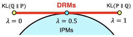
5.1 From DRM to the KL-divergence and the IPMs

We define a function class $\tilde{\mathcal{R}}$ as $\tilde{\mathcal{R}}=\left\{\exp(g(\cdot))\mid g\in\mathcal{G}\right\}$. Then, we obtain the following result.

Theorem 5.2.

Suppose that under $\mathcal{G}$, $\tilde{\mathcal{R}}$ satisfies Definition 3.2. Then,

$$\mathrm{DRM}^{1/2}_{\tilde{\mathcal{R}}}(\mathbb{P}\parallel\mathbb{Q})=\frac{1}{2}\mathrm{IPM}_{\mathcal{G}}(\mathbb{P}\parallel\mathbb{Q}).$$

Besides, suppose that $r^{*}\in\tilde{\mathcal{R}}$. If $\mathcal{W}_{q}\subseteq\mathcal{W}_{p}$, then $\mathrm{DRM}^{1}_{\tilde{\mathcal{R}}}(\mathbb{P}\parallel\mathbb{Q})=\mathrm{KL}(\mathbb{P}\parallel\mathbb{Q})$. If $\mathcal{W}_{p}\subseteq\mathcal{W}_{q}$, then $\mathrm{DRM}^{0}_{\tilde{\mathcal{R}}}(\mathbb{P}\parallel\mathbb{Q})=\mathrm{KL}(\mathbb{Q}\parallel\mathbb{P})$.

Thus, the DRMs bridge the IPMs and KL-divergence via the density ratio. We illustrate the concept in Figure 1.

In order to estimate the density ratio using finite samples, we need to control the roughness of the estimator appropriately, as explained in Section 3. In the DRMs, the problem of roughness can be considered as a choice of function class $\mathcal{R}$, which corresponds to the property of the IPMs that the different function class yields different metrics, such as Wasserstein distance and MMD.

Figure 1: Relationship between the KL-divergence, the IPMs, and DRMs. A family of the DRMs (red line) corresponds to the KL-divergence (yellow dots) at $\lambda\in\{0,1\}$, and is tangent to the set of the IPMs (blue region) at $\lambda=0.5$.

A map $d:\mathbb{P}\times\mathbb{Q}\mapsto d(\mathbb{P}\|\mathbb{Q})\in[0,\infty]$ is called a probability semimetric if it possesses the following properties: (i) $d(\mathbb{P}\parallel\mathbb{Q})=0$ if and only if $\mathbb{P}=\mathbb{Q}$; (ii) $d(\mathbb{P}\parallel\mathbb{Q})=d(\mathbb{Q}\parallel\mathbb{P})$; (iii) $d(\mathbb{P}\parallel\mathbb{Q})\leq d(\mathbb{P}\parallel\mathbb{O})+d(\mathbb{O}\parallel\mathbb{Q})$, where $\mathbb{O}$ is a probability measure. It is known that the IPMs are probability semimetric, and thus the following corollary holds.

Theorem 5.3.

Suppose the same condition in Theorem 5.2. Then, $\mathrm{DRM}^{1/2}_{\tilde{\mathcal{R}}}(\mathbb{P}\parallel\mathbb{Q})=\frac{1}{2}\mathrm{IPM}_{\mathcal{G}}(\mathbb{P}\parallel\mathbb{Q})$ is probability semimetric.

Table 1: Results of Section 6: means, medians, and stds of the squared error in DRE using synthetic datasets. The lowest mean and median (med) methods are highlighted in bold.

dim	uLSIF			RuLSIF $(\alpha=0.1)$			WD			DRM $(\lambda=0.5)$			DRM $(\lambda=0.1)$			DRM $(\lambda=0.9)$
	mean	med	std	mean	med	std	mean	med	std	mean	med	std	mean	med	std	mean	med	std
2	11.216	9.997	4.547	11.655	10.481	4.566	7.962	4.536	13.838	1.781	1.107	2.025	1.565	0.977	1.762	3.039	2.194	2.959
10	15.512	14.673	3.218	15.285	14.292	3.178	12.164	13.033	4.879	3.638	3.222	1.861	2.901	2.488	1.583	5.577	4.885	2.151
50	15.578	15.045	3.326	15.586	15.055	3.326	14.307	13.922	3.614	6.654	6.032	2.340	4.879	4.273	1.856	10.117	9.451	2.728
100	16.479	15.356	4.194	16.318	15.054	4.220	9.040	6.976	6.849	7.540	6.748	2.812	8.785	8.305	2.266	12.163	11.074	3.552

5.2 Topological Properties

We present topological properties of the DRMs, that is, their relation to weak convergence of probability distributions. Such the property is important for generative models, such as GANs and adversarial VAEs. Here, $\rightharpoonup$ denotes weak convergence of probability measures.

Theorem 5.4.

Let $\mathbb{P}$ be a probability measure and $(\mathbb{P}_{N})_{N\geq 0}$ be a sequence of probability measures. Suppose $\mathcal{W}$ is bounded. Then, we have the followings:

1. (imply weak convergence) For $\lambda\in[0,1]$, $\lim_{N\to\infty}\mathrm{DRM}^{\lambda}_{\mathcal{R}}(\mathbb{P}_{N}\parallel\mathbb{P})=0\Rightarrow\mathbb{P}_{N}\rightharpoonup\mathbb{P}$

2. (metrize weak convergence) For $\lambda=1/2$, $\lim_{N\to\infty}\mathrm{DRM}^{\lambda}_{\mathcal{R}}(\mathbb{P}_{N}\parallel\mathbb{P})=0\Leftrightarrow\mathbb{P}_{N}\rightharpoonup\mathbb{P}$.

The proof is provided in Appendix F.

5.3 GAN based on the DRMs

Given observations $\mathcal{X}$ from the density $p^{*}$, the goal of GANs is to learn a generator, which generates samples similar to $\mathcal{X}$. The generator is a parametric function $G_{\theta}:\mathbb{R}^{d^{\prime}}\to\mathcal{W}$, where $\theta\in\Theta$ is the parameter, $\Theta$ is the parameter space, and $d^{\prime}\ll d$. We denote the function class by $\{G_{\theta}\}_{\theta\in\Theta}$. Each function $G_{\theta}$ is applied to a $d^{\prime}$-dimensional random variable $\epsilon$, and for the generator, we define a family of densities $\mathcal{G}=\{q_{\beta}\}_{\beta\in\mathcal{B}}$. Let us denote $m\in\mathbb{N}$ i.i.d. samples drawn from the density $q_{\beta}$ by $\mathcal{W}_{q}$. In contrast, the discriminator $D$ belongs to a family of Borel functions from $\mathcal{W}$ to $(0,1)$, denoted by $\mathcal{D}$.

Probability divergence plays an important role in GANs, such as the Wasserstein GAN (Arjovsky et al., 2017; Bousquet et al., 2017) and MMD GAN. Based on the stratified MPL-DRE, we also propose Stratified Likelihood based GAN (SLoGAN). The SLoGAN train the generator and discriminator by solving the following minimax game:

$$\min_{\theta\in\Theta}\ \mathrm{DRM}^{\lambda}_{\mathcal{R}}(\mathbb{P}\parallel\mathbb{Q}_{\theta}).$$

Nguyen et al. (2017) proposes D2GAN with the following objective: $J(g,r_{1},r_{2})=\alpha\mathbb{E}_{p}\big{[}\log r_{1}(X_{i}))\big{]}-\mathbb{E}_{p}\big{[}r_{1}(X_{i}))\big{]}-\mathbb{E}_{q}\big{[}r_{2}(X_{i}))\big{]}+\beta\mathbb{E}_{p}\big{[}\log r(X_{i}))\big{]}$. This objective can be regarded as a variant of the DRMs and the IPMs. In Proposition 1 in Nguyen et al. (2017), the authors show that the optimal discriminator $r_{1}$ is $\alpha r^{*}$ and the optimal discriminator $r_{2}$ is $\beta/r^{*}$, if separate discriminators ($r_{1}=1/r_{2}$) and exponential density models are not used, the objective of D2GAN surprisingly can be reduced to a metric belonging to the IPMs under $\alpha=\beta=1$. For instance, if we use 1-Lipschitz functions for the class of the discriminators, the objective becomes the Wasserstein distance with the normalization constraints.

5.4 Related Work

DRE methods. Sugiyama et al. (2011b) and Kato and Teshima (2021) focus on the Bregman divergence (BD) minimization framework (Bregman, 1967) to provide a general framework that unifies various DRE methods, such as moment matching (Huang et al., 2007; Gretton et al., 2009), probabilistic classification (Qin, 1998; Cheng and Chu, 2004), density matching (Nguyen et al., 2008, 2010), density-ratio fitting (Kanamori et al., 2009), and learning from positive and unlabeled data (Kato et al., 2019).

More closely related to our work is the KLIEP, a framework of DRE by density matching under the KL divergence Sugiyama et al. (2008), Although the original implementation by Sugiyama et al. (2008) solves the constraint problem, we can transform the problem to an unconstrained problem by applying the method of Silverman (1982). The solution of KLIEP is equal to the solution of empirical UKL, $\min_{r\in\mathcal{R}}-\frac{1}{n}\sum^{n}_{i=1}\log r(X_{i})+\frac{1}{m}\sum^{m}_{j=1}r(Z_{j})$. Although Sugiyama et al. (2008, 2012) introduce the normalization constraint to this objective and omit $\frac{1}{m}\sum^{m}_{j=1}r(Z_{j})$, we do not have to conduct the transformation because the solution of the unconstrained problem satisfies the constraint.

The roughness problem is also closely related to the overfitting problem in DRE, called train-loss hacking (Kato and Teshima, 2021) and density-chasm problem (Rhodes et al., 2020). Rhodes et al. (2020), Ansari et al. (2020), Kumagai et al. (2021), and Choi et al. (2021) mainly focus on the support of two densities in population. On the other hand, Kato and Teshima (2021) considers that it is caused by the finite samples. The roughness problem is more related to the train-loss hacking because, as well as Good and Gaskins (1971), the estimated density ratio becomes a set of Dirac delta functions even if there is a common support between two densities, which causes the overfitting problem. We introduce the correction for our objective in Appendix G.

Relation to GANs. We discuss the generative ratio matching networks (Srivastava et al., 2020), which uses density ratio as a discriminator and use MMD to train the generator. Although they estimate the density ratio by using uLSIF by Kanamori et al. (2009), separately from the training generator with MMD, we can also estimate the density ratio from MMD; that is, based on our findings, we can train the discriminator and generator by using the same objective.

A density ratio is closely related to a discriminator in GANs (Tran et al., 2017). We can enforce the smoothness by using the findings of GANs. Chu et al. (2020) categorizes the smoothness of the discriminator, and find that we can enforce Lipschitz continuity by using some constraints, such as spectral normalization (Miyato et al., 2018).

6 Experiments

We empirically investigate the $L^{2}$ error $\|r-r^{*}\|_{L^{2}(\mathbb{Q})}$ in the proposed DRE based on DRM. We compare our DRM-based DRE with the uLSIF (Kanamori et al., 2009) and RuLSIF (Yamada et al., 2011). For DRM, we choose $\lambda$ from $0.5$, $0.9$, and $0.1$. The model is $3$-layer perceptron with a ReLU activation function, where the number of the nodes in the middle layer is $32$. We also apply the same spectral normalization (Miyato et al., 2018) to enforce Lipschitz continuity. Therefore, when setting $\lambda=0.5$ in DRM, the metric becomes WD with normalization constraints owing to Lipschitz continuity. We also show the results when we do not use the normalization constraints (just maximizing the log likelihood of MPL-DRE under the stratified sampling), denoted by WD. For uLSIF and RuLSIF, we use an open-source implementation, which uses a linear-in-parameter model with the Gaussian kernel (Kanamori et al., 2012). Let the dimensions of the domain be $d$, $\mathbb{P}=\mathcal{N}(\mu_{p},I_{d})$, and $\mathbb{Q}=\mathcal{N}(\mu_{q},I_{d})$, where $\mathcal{N}(\mu,\Sigma)$ denotes the multivariate normal distribution with mean $\mu$ and $\Sigma$, and let $\mu_{p}$ and $\mu_{q}$ be $d$-dimensional vectors $\mu_{p}=(0,0,\dots,0)^{\top}$ and $\mu_{q}=(1,0,\dots,0)^{\top}$, where and $I_{d}$ is a $d$-dimensional identity matrix. We fix the sample sizes at $n=m=1,000$ and choose $d$ from $\{2,10,50,100\}$. To measure the performance, we use the mean, median (med), and standard deviation (std) of the squared errors over $50$ trials. Note that in this setting, we know the true density ratio $r^{*}$. The results are shown in Table 1. The proposed DRM-based DRE methods estimate the density ratio more accurately than the other methods with a lower mean and median of the squared error. We also show additional experimental results with different parameters in Appendix H. From the additional results, we can find that appropriate choices of $\lambda$ lowers the squared error. Besides, we show experimental results on distribution modeling in Appendix I.

7 Conclusion

We have shown that the difference in sampling schemes in the construction of the likelihood of the density ratio yields the KL-divergence and the IPMs. Based on this finding, we have proposed a novel family of probability divergence, the DRMs, including the KL-divergence and the IPMs. In addition to DRE, the DRMs are useful in various applications; the present work has aimed to reach a deeper understanding through their connection to the density ratio.

Appendix A Proof of Theorem 3.3

Proof.

Preliminary, we define the following terms:

$$A(r)=-\int_{\mathcal{W}_{p}}\log(r(x))p^{*}(x)\mathrm{d}x+\int_{\mathcal{W}^{*}}r(z)q^{*}(z)\mathrm{d}z+\alpha\Psi(r),$$

$$A_{0}(r)=-\int_{\mathcal{W}_{p}}\log(r(x))p^{*}(x)\mathrm{d}x-\alpha\Psi(r).$$

Given $r$ in $\mathcal{R}$, we define $r^{\diamond}$ as

$$\log\left(r^{\diamond}(x)\right)=-\log\left(r(x)\right)-\log\left(\int_{\mathcal{W}^{*}}r(z)q^{*}(z)\mathrm{d}z+\int_{\mathcal{W}_{p}\cap\mathcal{W}^{c}_{q}}p^{*}(x)\mathrm{d}x\right).$$

Here, we have

$$r^{\diamond}(x)=\frac{r(x)}{\int_{\mathcal{W}^{*}}r(z)q^{*}(z)\mathrm{d}z+\int_{\mathcal{W}_{p}\cap\mathcal{W}^{c}_{q}}p^{*}(x)\mathrm{d}x}.$$

Therefore,

$$\int_{\mathcal{W}_{p}}r^{\diamond}(x)w^{*}(x)\mathrm{d}x=\int_{\mathcal{W}^{*}}r^{\diamond}(z)q^{*}(z)\mathrm{d}z+\int_{\mathcal{W}_{p}\cap\mathcal{W}^{c}_{q}}p^{*}(x)\mathrm{d}x=\frac{\int_{\mathcal{W}^{*}}r(z)q^{*}(z)\mathrm{d}z+\int_{\mathcal{W}_{p}\cap\mathcal{W}^{c}_{q}}p^{*}(x)\mathrm{d}x}{\int_{\mathcal{W}^{*}}r(z)q^{*}(z)\mathrm{d}z+\int_{\mathcal{W}_{p}\cap\mathcal{W}^{c}_{q}}p^{*}(x)\mathrm{d}x}=1,$$

where $w^{*}(x)=\mathbbm{1}[x\in\mathcal{W}^{*}](q^{*}(x)-p^{*}(x)/r^{\diamond}(x))+p^{*}(x)/r^{\diamond}(x)$. Besides, from the condition, $\Psi(r^{\diamond})=\Psi(r)$.

Using the equality, we obtain the following relation by elementary manipulations:

$$A\left(r^{\diamond}\right) =-\int_{\mathcal{W}_{p}}\log\left(r^{\diamond}(x)\right)p^{*}(x)\mathrm{d}x+\int_{\mathcal{W}^{*}}r^{\diamond}(z)q^{*}(z)\mathrm{d}z+\int_{\mathcal{W}_{p}\cap\mathcal{W}^{c}_{q}}p^{*}(x)\mathrm{d}x+\Psi(r^{\diamond})$$

$$=-\int_{\mathcal{W}_{p}}\left(\log\left(r(x)\right)-\log\left(\int_{\mathcal{W}^{*}}r(z)q^{*}(z)\mathrm{d}z+\int_{\mathcal{W}_{p}\cap\mathcal{W}^{c}_{q}}p^{*}(x)\mathrm{d}x\right)\right)p^{*}(x)\mathrm{d}x+1+\Psi(r)$$

$$=-\int_{\mathcal{W}_{p}}\log\left(r(x)\right)p^{*}(x)\mathrm{d}x+\log\left(\int_{\mathcal{W}^{*}}r(z)q^{*}(z)\mathrm{d}z+\int_{\mathcal{W}_{p}\cap\mathcal{W}^{c}_{q}}p^{*}(x)\mathrm{d}x\right)+1+\Psi(r)$$

$$=A(r)-\int_{\mathcal{W}^{*}}r(z)q^{*}(z)\mathrm{d}z-\int_{\mathcal{W}_{p}\cap\mathcal{W}^{c}_{q}}p^{*}(x)\mathrm{d}x+\log\left(\int_{\mathcal{W}^{*}}r(z)q^{*}(z)\mathrm{d}z+\int_{\mathcal{W}_{p}\cap\mathcal{W}^{c}_{q}}p^{*}(x)\mathrm{d}x\right)+1$$

$$=A(r)-T_{1}(r)+\log\left(T_{1}(r)\right)+1.$$

Hence, we obtain $A(r^{\diamond})\leq A(r)$. Also, $A(r^{\diamond})=A(r)$ holds only if $T_{1}(r)=1$, since $t-\log t\geq 1$ for all $t\geq 0$ and they are equal only if $t=1$.

Therefore, $r$ minimizes $A(r)$ if and only if $r$ minimizes $A(r)$ subject to $T_{1}(r)=1$. Here, note that, subject to $T_{1}(r)=1$, the two objectives $A(r)$ and $A_{0}(r)+1$ are identical. Thus, the proof is complete. ∎

Appendix B Proof of Theorem 3.4

Proof.

We consider the minimization of

$$-\int_{\mathcal{W}^{*}}\log(r(x))p^{*}(x)\mathrm{d}x+\int_{\mathcal{W}^{*}}r(z)q^{*}(z)\mathrm{d}z+\int_{\mathcal{W}_{p}\cap\mathcal{W}^{c}_{q}}p^{*}(x)\mathrm{d}x,$$

over all functions $r\in\mathcal{R}$. This problem can be reduced to the following point-wise minimization problem:

$$\min_{u\in(0,\infty)}-\log uq^{*}(x)+uq^{*}(x).$$ (8)

As we denote the solution by $u^{*}$, the first order condition of this minimization problem is given as

$$-\frac{1}{u^{*}}p^{*}(x)+q^{*}(x)=0,$$

and $u^{*}\in(0,\infty)$ holds. Then, the solution given as $u^{*}=\frac{p^{*}(x)}{q^{*}(x)}\in(0,\infty)$.

Finally, we define $r^{\dagger}_{\mathrm{ordinary},p}(x):=\operatorname*{arg\,min}_{u\in(0,\infty)}-\log uq^{*}(x)+uq^{*}(x)$ for $x\in\mathcal{W}^{*}$, $r^{\dagger}_{\mathrm{ordinary},p}(x)=r^{*}(x)$. From Definition 3.2, for $x\notin\mathcal{W}_{p}$, $r^{\dagger}_{\mathrm{ordinary},p}(x)=1/\overline{R}$, and for $x\notin\mathcal{W}_{q}$, $r^{\dagger}_{\mathrm{ordinary},p}(x)=\overline{R}$. It can be confirmed that $r^{\dagger}_{\mathrm{ordinary},p}(x)\in\mathcal{R}$ because $r^{*}$ is measurable and takes values in $(0,\infty)$. Therefore, the solution of the original optimization problem is equal to $r^{\dagger}_{\mathrm{ordinary},p}$ almost everywhere.

By the same procedure of the proof on $r^{\dagger}_{\mathrm{ordinary},p}$, we can obtain the $r^{\dagger}_{\mathrm{ordinary},q}$, which is equal to $r^{\dagger}_{\mathrm{ordinary},p}$. ∎

Appendix C Proof of Theorem 3.5

Proof.

Preliminary, we define some supportive notations:

$$\mathcal{K}(r)=\lambda\int\log r(x)\mathrm{d}\mathbb{P}(x)-(1-\lambda)\int\log r(x)\mathrm{d}\mathbb{Q}(x).$$

We consider the KKT condition for functionals. Let us consider minimizing $-\mathcal{K}(r)$ for $r\in\mathcal{R}$, where $\mathcal{R}$ is defined in Definition 3.2, satisfying $T_{1}(r)=T_{2}(r)=1$. We define a set of constrained functions as

$$\mathcal{T}_{1}:=\left\{r:T_{1}(r)=1\right\},\mbox{~{}~{}and~{}~{}}\mathcal{T}_{2}:=\left\{r:T_{2}(r)=1\right\}.$$

We consider the following inequality:

$$\min_{r\in\mathcal{R}\cap\mathcal{T}_{1}\cap\mathcal{T}_{2}}-\mathcal{K}(r) \geq\min_{r\in\mathcal{R}\cap\mathcal{T}_{1}\cap\mathcal{T}_{2}}-\lambda\int\log r(x)\mathrm{d}\mathbb{P}(x)+\min_{r\in\mathcal{R}\cap\mathcal{T}_{1}\cap\mathcal{T}_{2}}(1-\lambda)\int\log r(x)\mathrm{d}\mathbb{Q}(x)$$

$$\geq\min_{r\in\mathcal{R}\cap\mathcal{T}_{1}}-\lambda\int\log r(x)\mathrm{d}\mathbb{P}(x)+\min_{r\in\mathcal{R}\cap\mathcal{T}_{2}}(1-\lambda)\int\log r(x)\mathrm{d}\mathbb{Q}(x)$$ (9)

Then, we consider the solutions of

$$\min_{r\in\mathcal{R}\cap\mathcal{T}_{1}}-\int\log r(x)\mathrm{d}\mathbb{P}(x),$$

and

$$\min_{r\in\mathcal{R}\cap\mathcal{T}_{2}}-\int\log\frac{1}{r(x)}\mathrm{d}\mathbb{Q}(x),$$

where recall that we denote the solutions by $r^{\dagger}_{\mathrm{ordinary},p}(x)$ and $r^{\dagger}_{\mathrm{ordinary},q}(x)$.

First, Theorem 3.4 shows the solution $r^{\dagger}_{\mathrm{ordinary},p}$. This result can be applied to $r^{\dagger}_{\mathrm{ordinary},q}$. Then, we can confirm that $r^{\dagger}_{\mathrm{ordinary},p}(x)=r^{\dagger}_{\mathrm{ordinary}(x),q}=r^{\dagger}$. By definition, $r^{\dagger}$ satisfies the constraints in (9). Therefore, $r^{\dagger}_{\mathrm{ordinary},p}(x)=r^{\dagger}_{\mathrm{ordinary}(x),q}=r^{\dagger}$ is also the solution of (9). ∎

Appendix D Proof of Theorem 3.7

We consider relating the $L^{2}$ error bound to the DRM generalization error bound in the following lemma.

Lemma D.1 ($L^{2}$ distance bound).

Let $\mathcal{H}:=\{r:\mathcal{X}\to(0,\infty)|\int_{\mathcal{W}^{*}}|r(x)|^{2}\mathrm{d}x<\infty\}$ and assume $r^{*}\in\mathcal{H}$. If $\inf_{t\in(0,\infty)}br^{\prime\prime}(t)>0$, then there exists $\mu>0$ such that for all $r\in\mathcal{H}$,

$$\begin{split}&\lambda\|r-r^{*}\|_{L^{2}(\mathbb{Q})}^{2}/\|r^{*}\|^{2}_{L^{2}(\mathbb{P})}+(1-\lambda)\|1/r-1/r^{*}\|_{L^{2}(\mathbb{P})}^{2}/\|1/r^{*}\|^{2}_{L^{2}(\mathbb{Q})}\\ &=-2\left(\widetilde{\mathcal{K}}(r)-\widetilde{\mathcal{K}}(r^{*})\right)-o(\lambda\|r-r^{*}\|_{L^{2}(\mathbb{Q})}^{2})-o((1-\lambda)\|1/r-1/r^{*}\|_{L^{2}(\mathbb{P})}^{2}).\end{split}$$

Proof.

We define the additional notation

$$\widetilde{\mathcal{K}}(r)=\mathcal{K}(r)-(1-\lambda)\int_{\mathcal{W}^{*}}\frac{1}{r(x)}p^{*}(x)\mathrm{d}x-\lambda\int_{\mathcal{W}^{*}}r(z)q^{*}(z)\mathrm{d}z$$ .

Since $\mu:=\inf_{t\in(0,\infty)}\log^{\prime\prime}(t)>0$, the function $f$ is $\mu$-strongly convex. By the definition of strong convexity,

$$-\left(\widetilde{\mathcal{K}}(r)-\widetilde{\mathcal{K}}(r^{*})\right)$$

$$=-\lambda\int_{\mathcal{W}^{*}}\log r(x)\mathrm{d}\mathbb{P}(x)+(1-\lambda)\int_{\mathcal{W}^{*}}\log r(z)\mathrm{d}\mathbb{Q}(z)+(1-\lambda)\int_{\mathcal{W}^{*}}\frac{1}{r(x)}\mathrm{d}\mathbb{P}(x)+\lambda\int_{\mathcal{W}^{*}}r(z)\mathrm{d}\mathbb{Q}(z)-2$$

$$\ \ \ \ +\lambda\int_{\mathcal{W}^{*}}\log r^{*}(x)\mathrm{d}\mathbb{P}(x)-(1-\lambda)\int_{\mathcal{W}^{*}}\log r^{*}(z)\mathrm{d}\mathbb{Q}(z)-(1-\lambda)\int_{\mathcal{W}^{*}}\frac{1}{r^{*}(x)}\mathrm{d}\mathbb{P}(x)-\lambda\int_{\mathcal{W}^{*}}r^{*}(z)\mathrm{d}\mathbb{Q}(z)+2.$$

Here, we have

$$-\int_{\mathcal{W}^{*}}\log r(x)\mathrm{d}\mathbb{P}(x)+\int_{\mathcal{W}^{*}}r(z)\mathrm{d}\mathbb{Q}(z)+\int_{\mathcal{W}^{*}}\log r^{*}(x)\mathrm{d}\mathbb{P}(x)-\int_{\mathcal{W}^{*}}r^{*}(z)\mathrm{d}\mathbb{Q}(z)$$

$$=-\int_{\mathcal{W}^{*}}r^{*}(z)\log r(z)\mathrm{d}\mathbb{Q}(x)+\int_{\mathcal{W}^{*}}r(z)\mathrm{d}\mathbb{Q}(z)+\int_{\mathcal{W}^{*}}r^{*}(z)\log r^{*}(z)\mathrm{d}\mathbb{Q}(z)-\int_{\mathcal{W}^{*}}r^{*}(z)\mathrm{d}\mathbb{Q}(z)$$

$$=\int_{\mathcal{W}^{*}}\left\{-r^{*}(z)\log r(z)+r(z)+r^{*}(z)\log r^{*}(z)-r^{*}(z)\right\}\mathrm{d}\mathbb{Q}(z)$$

$$=\int_{\mathcal{W}^{*}}\left\{-r^{*}(z)\log\frac{r(z)}{r^{*}(z)}+r(z)-r^{*}(z)\right\}\mathrm{d}\mathbb{Q}(z)$$

$$=\int_{\mathcal{W}^{*}}\left\{-r^{*}(z)\left(\frac{r(z)}{r^{*}(z)}-1-\frac{1}{2}\left(\frac{r(z)}{r^{*}(z)}-1\right)^{2}+\cdots\right)+r(z)-r^{*}(z)\right\}\mathrm{d}\mathbb{Q}(z)$$

$$=\frac{1}{2}\int_{\mathcal{W}^{*}}\left(\frac{r(x)}{r^{*}(x)}-1\right)^{2}\mathrm{d}\mathbb{P}(x)+o\left(\int_{\mathcal{W}^{*}}\left(\frac{r(x)}{r^{*}(x)}-1\right)^{2}\mathrm{d}\mathbb{P}(x)\right).$$

Similarly,

$$\int_{\mathcal{W}^{*}}\log r(z)\mathrm{d}\mathbb{Q}(z)+\int_{\mathcal{W}^{*}}\frac{1}{r(x)}\mathrm{d}\mathbb{P}(x)-\log r^{*}(z)\mathrm{d}\mathbb{Q}(z)-\int_{\mathcal{W}^{*}}\frac{1}{r^{*}(x)}\mathrm{d}\mathbb{P}(x)$$

$$=\frac{1}{2}\int_{\mathcal{W}^{*}}\left(\frac{r^{*}(z)}{r(z)}-1\right)^{2}\mathrm{d}\mathbb{Q}(z)+o\left(\int_{\mathcal{W}^{*}}\left(\frac{r^{*}(z)}{r(z)}-1\right)^{2}\mathrm{d}\mathbb{Q}(z)\right).$$

By combining them,

$$-\left(\widetilde{\mathcal{K}}(r)-\widetilde{\mathcal{K}}(r^{*})\right)\geq\lambda/2\|r/r^{*}-1\|_{L^{2}(\mathbb{P})}^{2}+(1-\lambda)/2\|r^{*}/r-1\|_{L^{2}(\mathbb{Q})}^{2}+o(\|r/r^{*}-1\|_{L^{2}(\mathbb{P})}^{2})+o(\|r^{*}/r-1\|_{L^{2}(\mathbb{Q})}^{2}).$$

Here, from Hölder’s inequality,

$$\int_{\mathcal{W}^{*}}(r(x)-r^{*}(x))^{2}\mathrm{d}\mathbb{Q}(x) =\int_{\mathcal{W}^{*}}r^{*2}(x)\left(\frac{r(x)}{r^{*}(x)}-1\right)^{2}\mathrm{d}\mathbb{Q}(x)$$

$$=\int_{\mathcal{W}^{*}}r^{*}(z)\left(\frac{r(z)}{r^{*}(z)}-1\right)^{2}\mathrm{d}\mathbb{P}(z)\leq\|r^{*}\|^{2}_{L^{\infty}(\mathbb{P})}\|r/r^{*}-1\|_{L^{2}(\mathbb{P})}^{2}.$$

Similarly,

$$\int_{\mathcal{W}^{*}}(1/r(x)-1/r^{*}(x))^{2}\mathrm{d}\mathbb{Q}(x)\leq\|1/r^{*}\|^{2}_{L^{\infty}(\mathbb{Q})}\|r^{*}/r-1\|_{L^{2}(\mathbb{Q})}^{2}.$$

Therefore,

$$\begin{split}&\lambda\|r-r^{*}\|_{L^{2}(\mathbb{Q})}^{2}/\|r^{*}\|^{2}_{L^{\infty}(\mathbb{P})}+(1-\lambda)\|1/r-1/r^{*}\|_{L^{2}(\mathbb{P})}^{2}/\|1/r^{*}\|^{2}_{L^{\infty}(\mathbb{Q})}\\ &=-2\left(\widetilde{\mathcal{K}}(r)-\widetilde{\mathcal{K}}(r^{*})\right)-o(\lambda\|r-r^{*}\|_{L^{2}(\mathbb{Q})}^{2})-o((1-\lambda)\|1/r-1/r^{*}\|_{L^{2}(\mathbb{P})}^{2}).\end{split}$$

∎

Then, we prove Theorem 3.7 as follows:

Proof of Theorem 3.7.

Following Sugiyama et al. (2010, 2012), for $\mathbb{P}_{1},\mathbb{P}_{2}\in\mathcal{P}(\mathcal{W})$, we define unnormalized KL (UKL) objective functional as

$$\mathrm{UKL}(g;\mathbb{P}_{1},\mathbb{P}_{2})=1+\int g(x)\mathrm{d}\mathbb{P}_{1}(x)-\int\exp(g(x))\mathrm{d}\mathbb{P}_{2}(x).$$

Thanks to the strong convexity, by Lemma D.1, we have

$$\lambda\|\hat{r}-r^{*}\|_{L^{2}(\mathbb{Q})}^{2}/\|r^{*}\|^{2}_{L^{\infty}(\mathbb{P})}+(1-\lambda)\|1/\hat{r}-1/r^{*}\|_{L^{2}(\mathbb{P})}^{2}/\|1/r^{*}\|^{2}_{L^{\infty}(\mathbb{Q})}$$

$$=-\left(\widetilde{\mathcal{K}}(r)-\widetilde{\mathcal{K}}(r^{*})\right)-o(\lambda\|\hat{r}-r^{*}\|_{L^{2}(\mathbb{Q})}^{2})-o((1-\lambda)\|1/\hat{r}-1/r^{*}\|_{L^{2}(\mathbb{P})}^{2})$$

$$=\lambda\mathrm{UKL}(\hat{r})-\lambda\mathrm{UKL}(r^{*})+(1-\lambda)\mathrm{UKL}(1/\hat{r})-(1-\lambda)\mathrm{UKL}(1/r^{*})-o(\lambda\|\hat{r}-r^{*}\|_{L^{2}(\mathbb{Q})}^{2})-o((1-\lambda)\|1/\hat{r}-1/r^{*}\|_{L^{2}(\mathbb{P})}^{2}).$$

Here, we have

$$\mathrm{UKL}(\hat{r})-\mathrm{UKL}(r^{*})\underbrace{-\widehat{\mathrm{UKL}}(\hat{r})+\widehat{\mathrm{UKL}}(\hat{r})}_{\text{$=0$}}\underbrace{-\widehat{\mathrm{UKL}}(r^{*})+\widehat{\mathrm{UKL}}(r^{*})}_{\text{$=0$}}$$

$$\leq\underbrace{(\mathrm{UKL}(\hat{r})-\mathrm{UKL}(r^{*})+\widehat{\mathrm{UKL}}(r^{*})-\widehat{\mathrm{UKL}}(\hat{r}))}_{\text{$=:A$}},$$

where we used $\widehat{\mathrm{UKL}}(\hat{r})\leq\widehat{\mathrm{UKL}}(r^{*})$.

Let us define $\ell_{1}(r)$ and $\ell_{2}(r)$ as

$$\ell_{1}(r):=r,$$

$$\ell_{2}(r):=-\log r.$$

For a function $A:\mathcal{W}\to\mathbb{R}$, observations $\{W_{i}\}^{n}_{i=1}$, and a probability measure $\mathbb{W}$, let us denote the expectation and sample average by

$$\mathbb{E}_{\mathbb{W}}[A(W)]=\int_{\mathcal{W}^{*}}A(w)\mathrm{d}\mathbb{W}(w),$$

$$\widehat{\mathbb{E}}_{\mathbb{W}}[A(W)]=\frac{1}{n}\sum^{n}_{i=1}A(W_{i})=\int_{\mathcal{W}^{*}}A(w)\mathrm{d}\mathbb{W}_{n}(w),$$

where $\mathbb{W}_{b}:=n^{-1}\sum_{i=1}^{n}\delta_{W_{i}}$ is an empirical measure with $\{W_{i}\}_{i=1}^{n}$.

To bound $A$, for ease of notation, let $\ell_{1}^{r}=\ell_{1}(r(X))$ and $\ell_{2}^{r}=\ell_{2}(r(X))$. Then, since

$$\mathrm{UKL}(r) =\mathbb{E}_{\mathbb{Q}}\ell_{1}(r(X))+\mathbb{E}_{\mathbb{P}}\ell_{2}(r(X)),$$

$$\widehat{\mathrm{UKL}}(r) =\widehat{\mathbb{E}}_{\mathbb{Q}}\ell_{1}(r(X))+\widehat{\mathbb{E}}_{\mathbb{P}}\ell_{2}(r(X)),$$

we have

$$A =\mathrm{UKL}(\hat{r})-\mathrm{UKL}(r^{*})+\widehat{\mathrm{UKL}}(r^{*})-\widehat{\mathrm{UKL}}(\hat{r})$$

$$=(\mathbb{E}_{\mathbb{Q}}-\widehat{\mathbb{E}}_{\mathbb{Q}})(\ell_{1}^{\hat{r}}-\ell_{1}^{r^{*}})+(\mathbb{E}_{\mathbb{P}}-\widehat{\mathbb{E}}_{\mathbb{P}})(\ell_{2}^{\hat{r}}-\ell_{2}^{r^{*}})$$

$$\leq|(\mathbb{E}_{\mathbb{Q}}-\widehat{\mathbb{E}}_{\mathbb{Q}})(\ell_{1}^{\hat{r}}-\ell_{1}^{r^{*}})|+|(\mathbb{E}_{\mathbb{P}}-\widehat{\mathbb{E}}_{\mathbb{P}})(\ell_{2}^{\hat{r}}-\ell_{2}^{r^{*}})|$$

By applying Lemma D.3, for any $0<\gamma<2$, we have

$$A\leq O_{\mathbb{P}}\left(\max\left\{\frac{\|\hat{r}-r^{*}\|_{L^{2}(\mathbb{Q})}^{1-\gamma/2}}{\sqrt{\min\{n,m\}}},\frac{1}{(\min\{n,m\})^{2/(2+\gamma)}}\right\}\right).$$

Then, for any $0<\gamma<2$, we get

$$\mathrm{UKL}(\hat{r})-\mathrm{UKL}(r^{*})-o(\|r-r^{*}\|_{L^{2}(\mathbb{Q})}^{2})$$

$$=O_{\mathbb{P}}\left(\max\left\{\frac{\|\hat{r}-r^{*}\|_{L^{2}(\mathbb{Q})}^{1-\gamma/2}}{\sqrt{\min\{n,m\}}},\frac{1}{(\min\{n,m\})^{2/(2+\gamma)}}\right\}\right)-o(\|\hat{r}-r^{*}\|_{L^{2}(\mathbb{Q})}^{2}).$$

Similarly, we have

$$\mathrm{UKL}(1/\hat{r})-\mathrm{UKL}(1/r^{*})$$

$$=O_{\mathbb{P}}\left(\max\left\{\frac{\|1/\hat{r}-1/r^{*}\|_{L^{2}(\mathbb{P})}^{1-\gamma/2}}{\sqrt{\min\{n,m\}}},\frac{1}{(\min\{n,m\})^{2/(2+\gamma)}}\right\}\right)-o(\|1/\hat{r}-1/r^{*}\|_{L^{2}(\mathbb{P})}^{2}).$$

As a result, we have

$$\lambda\|\hat{r}-r^{*}\|_{L^{2}(\mathbb{Q})}^{2}/\|r^{*}\|^{2}_{L^{\infty}(\mathbb{P})}+(1-\lambda)\|1/\hat{r}-1/r^{*}\|_{L^{2}(\mathbb{P})}^{2}/\|1/r^{*}\|^{2}_{L^{\infty}(\mathbb{Q})}+o(\lambda\|\hat{r}-r^{*}\|_{L^{2}(\mathbb{Q})}^{2})-o((1-\lambda)\|1/\hat{r}-1/r^{*}\|_{L^{2}(\mathbb{P})}^{2})$$

$$=-2\left(\widetilde{\mathcal{K}}(r)-\widetilde{\mathcal{K}}(r^{*})\right)$$

$$=2\lambda O_{\mathbb{P}}\left(\max\left\{\frac{\|\hat{r}-r^{*}\|_{L^{2}(\mathbb{Q})}^{1-\gamma/2}}{\sqrt{\min\{n,m\}}},\frac{1}{(\min\{n,m\})^{2/(2+\gamma)}}\right\}\right)$$

$$\ \ \ +2(1-\lambda)O_{\mathbb{P}}\left(\max\left\{\frac{\|1/\hat{r}-1/r^{*}\|_{L^{2}(\mathbb{P})}^{1-\gamma/2}}{\sqrt{\min\{n,m\}}},\frac{1}{(\min\{n,m\})^{2/(2+\gamma)}}\right\}\right).$$

Here, we have

$$\min\left\{1/\|r^{*}\|^{2}_{L^{\infty}(\mathbb{P})},1/\|1/r^{*}\|^{2}_{L^{\infty}(\mathbb{Q})}\right\}\max\left\{\lambda\|\hat{r}-r^{*}\|_{L^{2}(\mathbb{Q})}^{2},(1-\lambda)\|1/\hat{r}-1/r^{*}\|_{L^{2}(\mathbb{P})}^{2}\right\}$$

$$\ \ \ +o(\max\left\{\lambda\|\hat{r}-r^{*}\|_{L^{2}(\mathbb{Q})}^{2},(1-\lambda)\|1/\hat{r}-1/r^{*}\|_{L^{2}(\mathbb{P})}^{2}\right\})$$

$$=O_{\mathbb{P}}\left(\max\left\{\max\left\{\frac{\lambda\|\hat{r}-r^{*}\|_{L^{2}(\mathbb{Q})}^{1-\gamma/2}}{\sqrt{\min\{n,m\}}},\frac{(1-\lambda)\|1/\hat{r}-1/r^{*}\|_{L^{2}(\mathbb{P})}^{1-\gamma/2}}{\sqrt{\min\{n,m\}}}\right\},\frac{1}{(\min\{n,m\})^{2/(2+\gamma)}}\right\}\right).$$

Consider a case where $\lambda\|\hat{r}-r^{*}\|_{L^{2}(\mathbb{Q})}^{2}\geq(1-\lambda)\|1/\hat{r}-1/r^{*}\|_{L^{2}(\mathbb{P})}^{2}$. In this case, we consider

$$\min\left\{1/\|r^{*}\|^{2}_{L^{\infty}(\mathbb{P})},1/\|1/r^{*}\|^{2}_{L^{\infty}(\mathbb{Q})}\right\}\lambda\|\hat{r}-r^{*}\|_{L^{2}(\mathbb{Q})}^{2}+o(\lambda\|\hat{r}-r^{*}\|_{L^{2}(\mathbb{Q})}^{2})$$

$$=O_{\mathbb{P}}\left(\max\left\{\frac{\lambda\|\hat{r}-r^{*}\|_{L^{2}(\mathbb{Q})}^{1-\gamma/2}}{\sqrt{\min\{n,m\}}},\frac{1}{(\min\{n,m\})^{2/(2+\gamma)}}\right\}\right).$$

Without loss of generality, we only consider a case where $\lambda>0$ and $\min\left\{1/\|r^{*}\|^{2}_{L^{\infty}(\mathbb{P})},1/\|1/r^{*}\|^{2}_{L^{\infty}(\mathbb{Q})}\right\}>0$. Then, because $\min\left\{1/\|r^{*}\|^{2}_{L^{\infty}(\mathbb{P})},1/\|1/r^{*}\|^{2}_{L^{\infty}(\mathbb{Q})}\right\}$ and $\lambda$ are constants, either

$$\|\hat{r}-r^{*}\|_{L^{2}(\mathbb{Q})}^{2}+o(\|\hat{r}-r^{*}\|_{L^{2}(\mathbb{Q})}^{2})=O_{\mathbb{P}}\left(\frac{\|\hat{r}-r^{*}\|_{L^{2}(\mathbb{Q})}^{1-\gamma/2}}{\sqrt{\min\{n,m\}}}\right),$$

or

$$\|\hat{r}-r^{*}\|_{L^{2}(\mathbb{Q})}^{2}+o(\|\hat{r}-r^{*}\|_{L^{2}(\mathbb{Q})}^{2})=O_{\mathbb{P}}\left(\frac{1}{(\min\{n,m\})^{2/(2+\gamma)}}\right),$$

holds. From the first case, we have the following result:

$$\|\hat{r}-r^{*}\|_{L^{2}(\mathbb{Q})}+o(\|\hat{r}-r^{*}\|_{L^{2}(\mathbb{Q})})=O_{\mathbb{P}}\left(\frac{1}{\min\{n,m\}^{1/(2+\gamma)}}\right).$$

From the second case, we have the following result:

$$\|\hat{r}-r^{*}\|_{L^{2}(\mathbb{Q})}+o(\|\hat{r}-r^{*}\|_{L^{2}(\mathbb{Q})})=O_{\mathbb{P}}\left(\frac{1}{(\min\{n,m\})^{1/(2+\gamma)}}\right).$$

In summary,

$$\lambda\|\hat{r}-r^{*}\|_{L^{2}(\mathbb{Q})}+o(\|\hat{r}-r^{*}\|_{L^{2}(\mathbb{Q})})=O_{\mathbb{P}}\left(\frac{1}{(\min\{n,m\})^{1/(2+\gamma)}}\right).$$

Similarly, for a case where $\lambda\|\hat{r}-r^{*}\|_{L^{2}(\mathbb{Q})}^{2}<(1-\lambda)\|1/\hat{r}-1/r^{*}\|_{L^{2}(\mathbb{P})}^{2}$, we have

$$(1-\lambda)\|\hat{r}-r^{*}\|_{L^{2}(\mathbb{P})}+o(\|\hat{r}-r^{*}\|_{L^{2}(\mathbb{P})})=O_{\mathbb{P}}\left(\frac{1}{(\min\{n,m\})^{1/(2+\gamma)}}\right).$$

By combining them,

$$\max\left\{\lambda\|\hat{r}-r^{*}\|_{L^{2}(\mathbb{Q})},(1-\lambda)\|1/\hat{r}-1/r^{*}\|_{L^{2}(\mathbb{P})}\right\}=O_{\mathbb{P}}\left(\frac{1}{(\min\{n,m\})^{1/(2+\gamma)}}\right).$$

∎

Each lemma used in the proof is provided as follows.

D.1 Bounding the Empirical Deviations

Following is a proposition originally presented in van de Geer (2000), which was rephrased in Kanamori et al. (2012) in a form that is convenient for our purpose.

Lemma D.2 (Lemma 5.13 in van de Geer (2000), Proposition 1 in Kanamori et al. (2012)).

Let $\mathcal{F}\subset L^{2}(\mathbb{P})$ be a function class and the map $I(f)$ be a complexity measure of $f\in\mathcal{F}$, where $I$ is a non-negative function on $\mathcal{F}$ and $I(f_{0})<\infty$ for a fixed $f_{0}\in\mathcal{F}$. We now define $\mathcal{F}_{M}=\{f\in\mathcal{F}:I(f)\leq M\}$ satisfying $\mathcal{F}=\bigcup_{M\geq 1}\mathcal{F}_{M}$. Suppose that there exist $c_{0}>0$ and $0<\gamma<2$ such that

$$\sup_{f\in\mathcal{F}_{M}}\|f-f_{0}\|\leq c_{0}M,\ \sup_{\stackrel{{\scriptstyle f\in\mathcal{F}_{M}}}{{\|f-f_{0}\|_{L^{2}(P)}\leq\delta}}}\|f-f_{0}\|_{\infty}\leq c_{0}M,\quad\text{for all }\delta>0,$$

and that $H_{B}(\delta,\mathcal{F}_{M},\mathbb{P})=O\left(M/\delta\right)^{\gamma}$. Then, we have

$$\sup_{f\in\mathcal{F}}\frac{\left|\int(f-f_{0})\mathrm{d}(\mathbb{P}-\mathbb{P}_{n})\right|}{D(f)}=O_{\mathbb{P}}\left(1\right),\ (n\to\infty),$$

where $D(f)$ is defined by

$$D(f)=\max\left\{\frac{\|f-f_{0}\|_{L^{2}(\mathbb{P})}^{1-\gamma/2}I(f)^{\gamma/2}}{\sqrt{n}},\frac{I(f)}{n^{2/(2+\gamma)}}\right\}.$$

Lemma D.3 (Lemma 10 in Kato and Teshima (2021)).

Under the conditions of Theorem 3.7, for any $0<\gamma<2$, we have

$$|(\mathbb{E}_{\mathbb{Q}}-\widehat{\mathbb{E}}_{\mathbb{Q}})(\ell_{1}^{\hat{r}}-\ell_{1}^{r^{*}})| =O_{\mathbb{P}}\left(\max\left\{\frac{\|\hat{r}-r^{*}\|_{L^{2}(\mathbb{Q})}^{1-\gamma/2}}{\sqrt{m}},\frac{1}{m^{2/(2+\gamma)}}\right\}\right)$$

$$|(\mathbb{E}_{\mathbb{P}}-\widehat{\mathbb{E}}_{\mathbb{P}})(\ell_{2}^{\hat{r}}-\ell_{2}^{r^{*}})| =O_{\mathbb{P}}\left(\max\left\{\frac{\|\hat{r}-r^{*}\|_{L^{2}(\mathbb{Q})}^{1-\gamma/2}}{\sqrt{n}},\frac{1}{n^{2/(2+\gamma)}}\right\}\right)$$

as $n,m\to\infty$.

D.2 Complexity of the hypothesis class

For the function classes in Definition D.5, we have the following evaluations of their complexities.

Lemma D.4 (Lemma 5 in Schmidt-Hieber (2020)).

For $L\in\mathbb{N}$ and $p\in\mathbb{N}^{L+2}$, let $V:=\prod_{l=0}^{L+1}(p_{l}+1)$. Then, for any $\delta>0$,

$$\log\mathcal{N}(\delta,\mathcal{H}(L,p,s,\infty),\|\cdot\|_{\infty})\leq(s+1)\log(2\delta^{-1}(L+1)V^{2}).$$

Definition D.5 (ReLU neural networks; Schmidt-Hieber, 2020).

For $L\in\mathbb{N}$ and $p=(p_{0},\ldots,p_{L+1})\in\mathbb{N}^{L+2}$,

$$\mathcal{F}(L,p):= \{f:x\mapsto W_{L}\sigma_{v_{L}}W_{L-1}\sigma_{v_{L-1}}\cdots W_{1}\sigma_{v_{1}}W_{0}x:$$

$$\qquad\qquad W_{i}\in\mathbb{R}^{p_{i+1}\times p_{i}},v_{i}\in\mathbb{R}^{p_{i}}(i=0,\ldots,L)\},$$

where $\sigma_{v}(y):=\sigma(y-v)$, and $\sigma(\cdot)=\max\{\cdot,0\}$ is applied in an element-wise manner. Then, for $s\in\mathbb{N},F\geq 0,L\in\mathbb{N}$, and $p\in\mathbb{N}^{L+2}$, define

$$\mathcal{H}(L,p,s,F):=\{f\in\mathcal{F}(L,p):\sum_{j=0}^{L}\|W_{j}\|_{0}+\|v_{j}\|_{0}\leq s,\|f\|_{\infty}\leq F\},$$

where $\|\cdot\|_{0}$ denotes the number of non-zero entries of the matrix or the vector, and $\|\cdot\|_{\infty}$ denotes the supremum norm. Now, fixing $\bar{L},\bar{p},s\in\mathbb{N}$ as well as $F>0$, we define

$$\mathrm{Ind}_{\bar{L},\bar{p}}:=\{(L,p):L\in\mathbb{N},L\leq\bar{L},p\in[\bar{p}]^{L+2}\},$$

and we consider the hypothesis class

$$\bar{\mathcal{H}} :=\bigcup_{(L,p)\in\mathrm{Ind}_{\bar{L},\bar{p}}}\mathcal{H}(L,p,s,F)$$

$$\mathcal{H} :=\{r\in\bar{\mathcal{H}}:\mathrm{Im}(r)\subset(b_{r},B_{r})\}.$$

Moreover, we define $I_{1}:\mathrm{Ind}_{\bar{L},\bar{p}}\to\mathbb{R}$ and $I:\mathcal{H}\to[0,\infty)$ by

$$I_{1}(L,p) :=2|\mathrm{Ind}_{\bar{L},\bar{p}}|^{\frac{1}{s+1}}(L+1)V^{2},$$

$$I(r) :=\max\left\{\|r\|_{\infty},\min_{\stackrel{{\scriptstyle(L,p)\in\mathrm{Ind}_{\bar{L},\bar{p}}}}{{r\in\mathcal{H}(L,p,s,F)}}}I_{1}(L,p)\right\},$$

where $V:=\prod_{l=0}^{L+1}(p_{l}+1)$, and we define

$$\mathcal{H}_{M}:=\{r\in\mathcal{H}:I(r)\leq M\}.$$

Proposition D.6 (Lemma 8 in Kato and Teshima (2021)).

There exists $c_{0}>0$ such that for any $\gamma>0$, any $\delta>0$, and any $M\geq 1$, we have

$$\log\mathcal{N}\left(\delta,\mathcal{H}_{M},\|\cdot\|_{\infty}\right) \leq\frac{s+1}{\gamma}\left(\frac{M}{\delta}\right)^{\gamma}.$$

and

$$\sup_{r\in\mathcal{H}_{M}}\|r-r^{*}\|_{\infty} \leq c_{0}M.$$

Definition D.7 (Derived function class and bracketing entropy).

Given a real-valued function class $\mathcal{F}$, define $\ell\circ\mathcal{F}:=\{\ell\circ f:f\in\mathcal{F}\}$. By extension, we define $I:\ell\circ\mathcal{H}\to[1,\infty)$ by $I(\ell\circ r)=I(r)$ and $\ell\circ\mathcal{H}_{M}:=\{\ell\circ r:r\in\mathcal{H}_{M}\}$. Note that, as a result, $\ell\circ\mathcal{H}_{M}$ coincides with $\{\ell\circ r\in\ell\circ\mathcal{H}:I(\ell\circ r)\leq M\}$.

Proposition D.8 (Lemma 9 in Kato and Teshima (2021)).

Let $\ell:(0,\infty)\to\mathbb{R}$ be a $\nu$-Lipschitz continuous function. Let $H_{B}\left(\delta,\mathcal{F},\|\cdot\|_{L^{2}(\mathbb{P})}\right)$ denote the bracketing entropy of $\mathcal{F}$ with respect to a distribution $\mathbb{P}$. Then, for any distribution $\mathbb{P}$, any $\gamma>0$, any $M\geq 1$, and any $\delta>0$, we have

$$H_{B}\left(\delta,\ell\circ\mathcal{H}_{M},\|\cdot\|_{L^{2}(\mathbb{P})}\right) \leq\frac{(s+1)(2\nu)^{\gamma}}{\gamma}\left(\frac{M}{\delta}\right)^{\gamma}.$$

Moreover, there exists $c_{0}>0$ such that for any $M\geq 1$ and any distribution $P$,

$$\sup_{\ell\circ r\in\ell\circ\mathcal{H}_{M}}\|\ell\circ r-\ell\circ r^{*}\|_{L^{2}(\mathbb{P})} \leq c_{0}\nu M,$$

$$\sup_{\stackrel{{\scriptstyle\ell\circ r\in\ell\circ\mathcal{H}_{M}}}{{\|\ell\circ r-\ell\circ r^{*}\|_{L^{2}(\mathbb{P})}\leq\delta}}}\|\ell\circ r-\ell\circ r^{*}\|_{\infty} \leq c_{0}\nu M,\quad\text{for all }\delta>0.$$

Appendix E Proof of Lemma 5.1

Proof.

We study two cases: (i) $\mathcal{W}_{p}=\mathcal{W}_{q}$, and (ii) $\mathcal{W}_{p}\neq\mathcal{W}_{q}$.

Consider the first case that $\mathcal{W}_{p}=\mathcal{W}_{q}$ holds. By Theorem 3.5, $\tilde{r}_{\mathrm{strat}}=r^{*}$ attains the maximum of $\mathrm{DRM}^{\lambda}_{\mathcal{R}}(\mathbb{P}\|\mathbb{Q})$. Hence, we have

$$\mathrm{DRM}^{\lambda}_{\mathcal{R}}(\mathbb{P}\|\mathbb{Q})=\lambda\mathrm{KL}(\mathbb{P}\|\mathbb{Q})+(1-\lambda)\mathrm{KL}(\mathbb{Q}\|\mathbb{P}).$$ (10)

Since the Kullback-Leibler divergence $\mathrm{KL}(\mathbb{P}\|\mathbb{Q})$ satisfies $\mathrm{KL}(\mathbb{P}\|\mathbb{Q})=0\Leftrightarrow\mathbb{P}=\mathbb{Q}$, we obtain the statement.

Consider the second case $\mathcal{W}_{q}\neq\mathcal{W}_{q}$. In this case, we always have $\mathbb{P}\neq\mathbb{Q}$, hence it is sufficient to show that $\mathrm{DRM}^{\lambda}_{\mathcal{R}}(\mathbb{P}\|\mathbb{Q})>0$. We substitute $r^{\dagger}_{\mathrm{strat}}$ and obtain

$$\mathrm{DRM}^{\lambda}_{\mathcal{R}}(\mathbb{P}\|\mathbb{Q}) \geq\mathcal{K}(r^{\dagger}_{\mathrm{strat}})$$

$$=\lambda\int_{\mathcal{W}^{*}}\log r^{*}(x)\mathrm{d}\mathbb{P}(x)+(1-\lambda)\int_{\mathcal{W}^{*}}\log(1/r^{*}(x))\mathrm{d}\mathbb{Q}(x)$$

$$\quad+\lambda\int_{\mathcal{W}_{p}\backslash\mathcal{W}_{q}}\log\overline{R}\mathrm{d}\mathbb{P}(x)+(1-\lambda)\int_{\mathcal{W}_{q}\backslash\mathcal{W}_{p}}\log\overline{R}\mathrm{d}\mathbb{Q}(x).$$

We have

$$\int_{\mathcal{W}^{*}}\log r^{*}(x)\mathrm{d}\mathbb{P}(x) =\int_{\mathcal{W}^{*}}-\log\left(\frac{q^{*}(x)}{p^{*}(x)}\right)\mathrm{d}\mathbb{P}(x)$$

$$\geq\int_{\mathcal{W}^{*}}-\left(\frac{q^{*}(x)}{p^{*}(x)}-1\right)\mathrm{d}\mathbb{P}(x)$$

$$=\int_{\mathcal{W}^{*}}\left(p^{*}(x)-q^{*}(x)\right)\mathrm{d}x$$

$$=\mathbb{P}(\mathcal{W}^{*})-\mathbb{Q}(\mathcal{W}^{*}),$$

where the inequality follows $\log(x)\leq(x-1)$. Using this inequality, we continue the lower bound on $\mathrm{DRM}^{\lambda}_{\mathcal{R}}(\mathbb{P}\|\mathbb{Q})$ as

$$\mathrm{DRM}^{\lambda}_{\mathcal{R}}(\mathbb{P}\|\mathbb{Q})$$

$$\geq\lambda(\mathbb{P}(\mathcal{W}^{*})-\mathbb{Q}(\mathcal{W}^{*}))+(1-\lambda)(\mathbb{Q}(\mathcal{W}^{*})-\mathbb{P}(\mathcal{W}^{*}))$$

$$\quad+(\lambda\mathbb{P}(\mathcal{W}_{p}\backslash\mathcal{W}_{q})+(1-\lambda)\mathbb{Q}(\mathcal{W}_{q}\backslash\mathcal{W}_{p}))\log\overline{R}$$

$$=(2\lambda-1)\mathbb{P}(\mathcal{W}^{*})+(1-2\lambda)\mathbb{Q}(\mathcal{W}^{*})+(\lambda\mathbb{P}(\mathcal{W}_{p}\backslash\mathcal{W}_{q})+(1-\lambda)\mathbb{Q}(\mathcal{W}_{q}\backslash\mathcal{W}_{p}))\log\overline{R}.$$

We show that the lower bound is strictly positive. For $\lambda\in[0,1/2]$, the lower bound is larger than $0$ if

$$\log\overline{R}>\frac{(1-2\lambda)(\mathbb{P}(\mathcal{W}^{*})-\mathbb{Q}(\mathcal{W}^{*}))}{\lambda\mathbb{P}(\mathcal{W}_{p}\backslash\mathcal{W}_{q})+(1-\lambda)\mathbb{Q}(\mathcal{W}_{q}\backslash\mathcal{W}_{p})}$$

holds. Similarly, for $\lambda\in[1/2,1]$, we obtain the same result when we have

$$\log\overline{R}>\frac{(2\lambda-1)(\mathbb{Q}(\mathcal{W}^{*})-\mathbb{P}(\mathcal{W}^{*}))}{\lambda\mathbb{P}(\mathcal{W}_{p}\backslash\mathcal{W}_{q})+(1-\lambda)\mathbb{Q}(\mathcal{W}_{q}\backslash\mathcal{W}_{p})}.$$

Note that $\min\{\mathbb{P}(\mathcal{W}_{p}\backslash\mathcal{W}_{q}),\mathbb{Q}(\mathcal{W}_{q}\backslash\mathcal{W}_{p})\}>0$ holds by the setting. Hence, if $\overline{R}$ is sufficiently large such that satisfies the inequalities, we show that $\mathrm{DRM}^{\lambda}_{\mathcal{R}}(\mathbb{P}\|\mathbb{Q})>0$. ∎

Appendix F Proof of Theorem 5.4

Proof.

We show the statements one by one.

1: We put $r^{*}$ in the maximum in $\mathrm{DRM}^{\lambda}_{\mathcal{R}}(\mathbb{P}\|\mathbb{Q})$ and obtain

$$\mathrm{DRM}^{\lambda}_{\mathcal{R}}(\mathbb{P}\|\mathbb{Q}) \geq\lambda\int_{\mathcal{W}_{p}}\log(r^{*}(x))\mathrm{d}\mathbb{P}(x)+(1-\lambda)\int_{\mathcal{W}_{q}}\log(1/r^{*}(x))\mathrm{d}\mathbb{Q}(x)$$

$$=\lambda\mathrm{KL}(\mathbb{P}\|\mathbb{Q})+(1-\lambda)\mathrm{KL}(\mathbb{Q}\|\mathbb{P}).$$

Hence, we have $\limsup_{N\to\infty}\lambda\mathrm{KL}(\mathbb{P}_{N}\|\mathbb{P})+(1-\lambda)\mathrm{KL}(\mathbb{P}\|\mathbb{P}_{N})=0$. Combining the non-negativity of the Kullback-Leibler divergence, we obtain $\lim_{n\to\infty}\mathrm{KL}(\mathbb{P}_{N}\|\mathbb{P})$ and $\lim_{n\to\infty}\mathrm{KL}(\mathbb{P}\|\mathbb{P}_{N})=0$. Since the Kullback-Leibler divergence implies weak convergence (Gibbs and Su, 2002) with the bounded assumption, we obtain the statement.

2: The direction $\Rightarrow$ follows the above first statement. We show the opposite $\Leftarrow$. With $\lambda=1/2$, we obtain

$$\mathrm{DRM}^{1/2}_{\mathcal{R}}(\mathbb{P}_{N}\|\mathbb{P})=\frac{1}{2}\sup_{r\in C(\mathcal{R})}\left\{\int_{\mathcal{W}}\log r(x)\mathrm{d}(\mathbb{P}_{N}-\mathbb{P})(x)\right\}.$$

Since $r\in C(\mathcal{R})$ is a continuous, bounded, and strictly positive function, $\log r$ is continuous and bounded. Hence, by the definition of weak convergence, we obtain the statement. ∎

Algorithm 1 nnDRM

  Input: Training data $\big{\{}X_{i}\big{\}}^{n}_{i=1}$ and $\big{\{}Z_{j}\big{\}}^{m}_{j=1}$, the algorithm for stochastic optimization such as Adam (Kingma and Ba, 2015), the learning rate $\gamma$, the regularization coefficient $\lambda$ and function $\mathcal{R}(r)$, and a constant $C>0$.

  Output: A density ratio estimator $\hat{r}$.

  while No stopping criterion has been met: do

     $N$ mini-batches: $\big{\{}\big{(}\big{\{}X^{k}_{i}\big{\}}^{n_{k}}_{i=1},\big{\{}Z^{k}_{j}\big{\}}^{m_{k}}_{j=1}\big{)}\big{\}}^{N}_{k=1}.$

     for $k=1$ to $N$ do

        if $\sum^{m_{k}}_{j=1}r(Z^{k}_{j})-C\sum^{n_{k}}_{i=1}r(X^{k}_{i})\geq 0$: then

           Gradient decent: set gradient

$$\mathrm{Grad}=\nabla_{r}\widehat{\mathrm{nnUKL}}(r,\mathbb{P}^{k}_{n},\mathbb{Q}^{k}_{n}).$$

        else

           Gradient ascent: set gradient

$$\mathrm{Grad}=\nabla_{r}\big{\{}\sum^{m_{k}}_{j=1}r(Z^{k}_{j})-C\sum^{n_{k}}_{i=1}r(X^{k}_{i})\big{\}}.$$

        end if

        if $\sum^{n_{k}}_{i=1}\frac{1}{r(X^{k}_{i})}-C\sum^{m_{k}}_{j=1}\frac{1}{r(Z^{k}_{j})}\geq 0$: then

           Gradient decent: add gradient

$$\mathrm{Grad}\mathrel{{+}{=}}\nabla_{r}\widehat{\mathrm{nnUKL}}(\frac{1}{r},\mathbb{Q}^{k}_{n},\mathbb{P}^{k}_{n}).$$

        else

           Gradient ascent: add gradient

$$\mathrm{Grad}\mathrel{{+}{=}}\nabla_{r}\big{\{}\sum^{n_{k}}_{i=1}\frac{1}{r(X^{k}_{i})}-C\sum^{m_{k}}_{j=1}\frac{1}{r(Z^{k}_{j})}\big{\}}.$$

        end if

        Update $r$ with the gradient and the learning rate $\gamma$.

     end for

  end while

Appendix G Estimation of the DRM and Density Ratio

We can estimate the density ratio by solving the inner maximization problem in DRM; that is, we consider minimizing

$$\widehat{\mathcal{K}}(r)=\Bigg{\{}\lambda\frac{1}{n}\sum^{n}_{i=1}\log r(X_{i})-(1-\lambda)\frac{1}{m}\sum^{m}_{j=1}\log r(Z_{j})-\frac{1-\lambda}{n}\sum^{n}_{i=1}\frac{1}{r(X_{i})}-\frac{\lambda}{m}\sum^{m}_{j=1}r(Z_{j})\Bigg{\}},$$

Besides, if we know the upper bounds of $r^{*}$ and $1/r^{*}$, we can also impose the non-negative correction proposed by Kiryo et al. (2017) and Kato and Teshima (2021). In UKL , does not become negative because… Based on this motivation. Kato and Teshima (2021) proposes the following nonnegative UKL:

$$\widehat{\mathrm{nnUKL}}(r):=-\sum^{n}_{i=1}\Big{(}\log\big{(}r(X_{i})\big{)}-Cr(X_{i})\Big{)}+\left(\sum^{m}_{j=1}r(Z_{j})-C\sum^{n}_{i=1}r(X_{i})\right)_{+},$$

where $C$. Note that if $\overline{R}=\infty$, $C=0$ and the second term is always positive. Therefore, the nonnegative UKL is identical to the original UKL. Thus, we can regard nonnegative UKL is a generalization of the original UKL.

The empirical counterpart of the nonnegative UKL is given as

$$\widehat{\mathrm{nn}\mathcal{K}}(r)=\lambda\widehat{\mathrm{nnUKL}}(r,\mathbb{P}_{n},\mathbb{Q}_{m})-(1-\lambda)\widehat{\mathrm{nnUKL}}(1/r,\mathbb{Q}_{m}.\mathbb{P}_{n}),$$

When the nonnegative correction is violated, instead of simply replacing it with $0$, we can use gradient ascent; that is, if … The use of gradient ascent is reported to improve the empirical performance Kiryo et al. (2017); Kato and Teshima (2021). Our proposed algorithm is summarized in Algorithm 1.

Table 2: Results of Appendix H: means, medians, and stds of the squared error in DRM-based DRE using synthetic datasets. The lowest mean and median (med) methods are highlighted in bold.

sample sizes: $n=1000$, $m=100$
dim	$\lambda=0.0$			$\lambda=0.2$			$\lambda=0.4$			$\lambda=0.6$			$\lambda=0.8$			$\lambda=1,0$
	mean	med	std	mean	med	std	mean	med	std	mean	med	std	mean	med	std	mean	med	std
10	8.129	6.045	8.444	8.969	6.699	9.371	9.843	7.467	9.778	10.867	8.464	9.954	11.915	9.384	10.315	12.874	10.224	10.584
100	26.693	26.407	6.058	18.115	16.749	5.663	12.581	12.130	3.165	14.481	13.816	3.439	16.296	15.637	3.520	17.145	16.438	3.554
sample sizes: $n=10000$, $m=100$
dim	$\lambda=0.0$			$\lambda=0.2$			$\lambda=0.4$			$\lambda=0.6$			$\lambda=0.8$			$\lambda=1,0$
	mean	med	std	mean	med	std	mean	med	std	mean	med	std	mean	med	std	mean	med	std
10	3.458	3.338	1.202	3.767	3.729	1.143	4.088	4.148	1.146	4.669	4.562	1.208	5.518	5.608	1.134	6.71	6.479	1.167
100	6.748	6.608	1.138	6.886	6.759	1.213	8.157	8.028	1.348	10.579	10.329	1.443	12.502	12.303	1.522	13.71	13.578	1.506
sample sizes: $n=10000$, $m=100$
dim	$\lambda=0.0$			$\lambda=0.2$			$\lambda=0.4$			$\lambda=0.6$			$\lambda=0.8$			$\lambda=1,0$
	mean	med	std	mean	med	std	mean	med	std	mean	med	std	mean	med	std	mean	med	std
0	6.735	6.445	1.537	7.221	7.134	1.750	8.069	7.931	1.576	9.099	8.999	1.558	10.148	10.026	1.503	10.975	10.854	1.531
1	15.215	14.857	2.579	11.843	11.674	1.304	11.556	11.434	1.279	14.722	14.514	1.288	16.499	16.329	1.267	17.267	17.206	1.293

Appendix H Additional Results of Section 6

In addition to the experimental results shown in Section 6, we investigate the performance of the DRM-based DRE with different $\lambda$, chosen from $\{0.0,0.2,0.4,0.6,0.8,1.0\}$.

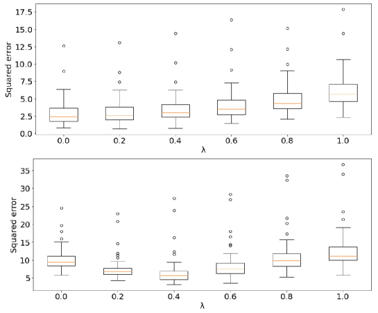
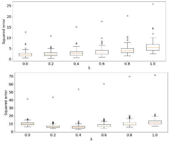
First, we change the sample sizes. We show the results with sample sizes $(n,m)=(1000,100)$, $(n,m)=(10000,1000)$, and $(n,m)=(10000,100)$ in Table 2. We choose the dimension $d$ from $\{10,100\}$. The other settings are identical to that of Section 6. In Section 6, DRM with $\lambda=0.9$ achieves the lowest mean and squared errors. However, in this result, DRM with $\lambda=0.5$ achieves lower mean and squared errors than that with $\lambda=0.9$. We consider that this is because balancing $lambda$ between the log likelihood of the density ratio and inverse density ratio makes the estimation error lower as discussed in Wooldridge (2001). In this case, because $n$ is larger than $m$. Therefore, weighting the log likelihood $\frac{1}{n}\sum^{n}_{i=1}\log r(X_{i})$ more than $\frac{1}{m}\sum^{m}_{j=1}\log\frac{1}{r(X_{i})}$ may make the estimation more accurate.

Next, we change the mean vectors from the setting of Section 6 as $\mu_{p}=(1,0,\dots,0)^{\top}$ and $\mu_{q}=(0,0,\dots,0)^{\top}$. The other settings are the same as that of Section 6. The results shown by boxplots in Figures 3 and 3.

It can be confirmed that the error can be reduced by adjusting $\lambda$ appropriately. For example, in Section 6, DRM with $\lambda=0.1$ shows the best performance. However, by observing the results carefully, we can find that there are cases where setting $lambda$ around $0,4$ may reduce the error more than setting with $\lambda=0$. We can also find that appropriate choices of $\lambda$ are also affected by the changes in the sample size ratio and the mean vectors.

Table 3: Negative Log-likelihood (NLL) and MMD, multiplied by $10^{3}$, results on six 2-d synthetic datasets. Lower is better.

Metric	GAN	MoG	Banana	Rings	Square	Cosine	Funnel
NLL	WGAN	$\bm{-2.59\pm 0.04}$	$-3.58\pm 0.00$	$\bm{-4.26\pm 0.00}$	$-3.74\pm 0.00$	$-3.99\pm 0.00$	$\bm{-3.58\pm 0.01}$
	KL-WGAN	$-2.55\pm 0.01$	$\bm{-3.59\pm 0.01}$	$-4.25\pm 0.01$	$\bm{-3.73\pm 0.01}$	$\bm{-4.00\pm 0.02}$	$-3.57\pm 0.01$
	SLoGAN	$-2.52\pm 0.01$	$-3.58\pm 0.00$	$\bm{-4.26\pm 0.00}$	$-3.71\pm 0.01$	$-3.99\pm 0.00$	$-3.57\pm 0.00$
MMD	WGAN	$16.38\pm 7.47$	$2.32\pm 0.80$	$1.73\pm 0.30$	$1.48\pm 0.39$	$1.08\pm 0.32$	$1.83\pm 0.72$
	KL-WGAN	$\bm{2.26\pm 0.22}$	$1.96\pm 0.12$	$\bm{1.34\pm 0.23}$	$1.35\pm 0.21$	$\bm{1.00\pm 0.13}$	$\bm{1.16\pm 0.31}$
	SLoGAN	$5.89\pm 1.49$	$\bm{1.38\pm 0.43}$	$1.79\pm 0.37$	$\bm{0.73\pm 0.09}$	$1.10\pm 0.24$	$1.63\pm 0.32$

Appendix I Experimental on Distribution Modeling

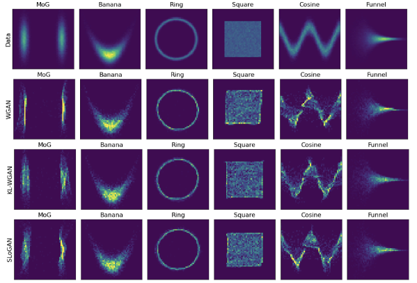
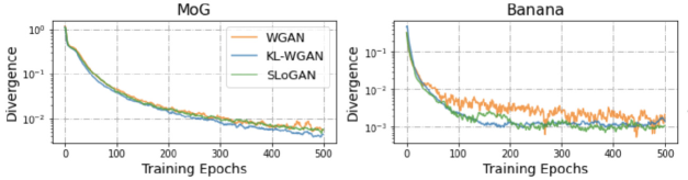
We investigate the distribution modeling using DRM. Following Song and Ermon (2020), we use the 2-d synthetic datasets include Mixture of Gaussians (MoG), Banana, Ring, Square, Cosine and Funnel; these datasets cover different modalities and geometries. We compare our proposed DRM with the WGAN and KL-WGAN, proposed by Song and Ermon (2020).

After training, we draw 5,000 samples from the generator and then evaluate two metrics over a fixed validation set. One is the negative log-likelihood (NLL) of the validation samples on a kernel density estimator fitted over the generated samples; the other is the MMD (Borgwardt et al. (2006)) between the generated samples and validation samples. To ensure a fair comparison, we use identical kernel bandwidths for all cases.

Distribution modeling.

We report the mean and standard error for the NLL and MMD results in Tables 3 (with 5 random seeds in each case). We illustrate the histograms of samples in Figure 6.

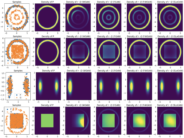
Density ratio estimation.

We demonstrate that SLoGAN learns the density ratio simultaneously. We consider measuring the density ratio from synthetic datasets, and compare them with the the discriminators of WGAN, $f$-GAN with KL divergence, KL-WGAN. We evaluate the density ratio estimation quality by multiplying $\mathrm{d}\mathbb{Q}$ with the estimated density ratios, and compare that with the density of $\mathbb{P}$; ideally the two quantities should be identical. We demonstrate empirical results in Figure 6, where we plot the samples used for training, the ground truth density $p^{*}$ and the two estimates given by two methods. In terms of estimating density ratios, our proposed approach estimates it as well as f-GAN and KL-WGAN.

Stability of discriminator objectives.

For the MoG and Square and Cosine datasets, we further show the estimated divergences over a batch of 256 samples in Figure 6. While divergences of KL-WGAN and our proposed SLoGAN decrease more stable tan that of WGAN.

Figure 2: Results of Appendix H: The mean vectors are $\mu_{p}=(0,0,\dots,0)^{\top}$ and $\mu_{q}=(1,0,\dots,0)^{\top}$.

Figure 3: Results of Appendix H: The mean vectors are $\mu_{p}=(1,0,\dots,0)^{\top}$ and $\mu_{q}=(0,0,\dots,0)^{\top}$.

Figure 4: Results of Appendix I: Histograms of samples from the true data distribution, WGAN and KL-WGAN, and our SLoGAN

Figure 5: Results of Appendix I: Estimating density ratios. The first column contains the samples used for training, the second column is the ground truth density of $\mathbb{P}$ ($p^{*}$), the third and sixth columns are the density of $\mathbb{Q}$ times the estimated density ratios from WGAN (thrid column), f-GAN (fourth column), KL-WGAN (fifth column), and our SLoGAN (sixth column).

Figure 6: Results of Appendix I: Estimated divergence with respect to training epochs (smoothed with a window of $10$).

References

• Abe and Sugiyama (2019) Abe, M. and Sugiyama, M. (2019), “Anomaly Detection by Deep Direct Density Ratio Estimation,” openreview.
• Agrawal and Horel (2020) Agrawal, R. and Horel, T. (2020), “Optimal Bounds between f-Divergences and Integral Probability Metrics,” in International Conference on Machine Learning, eds. III, H. D. and Singh, A., vol. 119, pp. 115–124.
• Ali and Silvey (1966) Ali, S. M. and Silvey, S. D. (1966), “A general class of coefficients of divergence of one distribution from another,” Journal of the Royal Statistical Society, Series B, 131–142.
• Ambrosio et al. (2005) Ambrosio, L., Gigli, N., and Savare, G. (2005), Gradient Flows: In Metric Spaces and in the Space of Probability Measures, Lectures in Mathematics. ETH Zürich, Birkhäuser Basel.
• Ansari et al. (2020) Ansari, A. F., Ang, M. L., and Soh, H. (2020), “Refining Deep Generative Models via Wasserstein Gradient Flows,” in International Conference on Learning Representations.
• Arbel et al. (2021) Arbel, M., Zhou, L., and Gretton, A. (2021), “Generalized Energy Based Models,” in International Conference on Learning Representations.
• Arjovsky et al. (2017) Arjovsky, M., Chintala, S., and Bottou, L. (2017), “Wasserstein GAN,” .
• Belavkin (2018) Belavkin, R. V. (2018), “Relation Between the Kantorovich–Wasserstein Metric and the Kullback–Leibler Divergence,” in Information Geometry and Its Applications, Cham: Springer International Publishing, pp. 363–373.
• Borgwardt et al. (2006) Borgwardt, K. M., Gretton, A., Rasch, M. J., Kriegel, H.-P., Schölkopf, B., and Smola, A. J. (2006), “Integrating structured biological data by Kernel Maximum Mean Discrepancy,” Bioinformatics, 22, e49–e57.
• Bousquet et al. (2017) Bousquet, O., Gelly, S., Tolstikhin, I., Simon-Gabriel, C.-J., and Schoelkopf, B. (2017), “From optimal transport to generative modeling: the VEGAN cookbook,” .
• Bregman (1967) Bregman, L. (1967), “The relaxation method of finding the common point of convex sets and its application to the solution of problems in convex programming,” USSR Computational Mathematics and Mathematical Physics, 7, 200 – 217.
• Cheng and Chu (2004) Cheng, k.-F. and Chu, C. (2004), “Semiparametric density estimation under a two-sample density ratio model,” Bernoulli, 10.
• Chernozhukov et al. (2016) Chernozhukov, V., Escanciano, J. C., Ichimura, H., Newey, W. K., and Robins, J. M. (2016), “Locally Robust Semiparametric Estimation,” .
• Choi et al. (2021) Choi, K., Liao, M., and Ermon, S. (2021), “Featurized density ratio estimation,” in Conference on Uncertainty in Artificial Intelligence, vol. 161, pp. 172–182.
• Chu et al. (2020) Chu, C., Minami, K., and Fukumizu, K. (2020), “Smoothness and Stability in GANs,” in International Conference on Learning Representations.
• Csiszár (1967) Csiszár, I. (1967), “Information-type measures of difference of probability distributions and indirect observation,” Studia Scientiarum Mathematicarum Hungarica.
• de Montricher et al. (1975) de Montricher, G. F., Tapia, R. A., and Thompson, J. R. (1975), “Nonparametric Maximum Likelihood Estimation of Probability Densities by Penalty Function Methods,” The Annals of Statistics, 3, 1329 – 1348.
• Donsker and Varadhan (1976) Donsker, M. D. and Varadhan, S. R. S. (1976), “Asymptotic evaluation of certain Markov process expectations for large time—III,” Communications on Pure and Applied Mathematics, 29, 389–461.
• Dudley (2002) Dudley, R. M. (2002), Real Analysis and Probability, Cambridge Studies in Advanced Mathematics, Cambridge University Press, 2nd ed.
• Eggermont and LaRiccia (1999) Eggermont, P. P. B. and LaRiccia, V. N. (1999), “Optimal convergence rates for Good’s nonparametric maximum likelihood density estimator,” The Annals of Statistics, 27, 1600 – 1615.
• Fang et al. (2020) Fang, T., Lu, N., Niu, G., and Sugiyama, M. (2020), “Rethinking Importance Weighting for Deep Learning under Distribution Shift,” in Conference on Neural Information Processing Systems.
• Gibbs and Su (2002) Gibbs, A. L. and Su, F. E. (2002), “On choosing and bounding probability metrics,” International statistical review, 70, 419–435.
• Glaser et al. (2021) Glaser, P., Arbel, M., and Gretton, A. (2021), “KALE Flow: A Relaxed KL Gradient Flow for Probabilities with Disjoint Support,” in Conference on Neural Information Processing Systems.
• Good (1971) Good, I. J. (1971), “Non-parametric Roughness Penalty for Probability Densities,” Nature Physical Science, 229, 29–30.
• Good and Gaskins (1971) Good, I. J. and Gaskins, R. A. (1971), “Nonparametric Roughness Penalties for Probability Densities,” Biometrika, 58, 255–277.
• Goodfellow et al. (2014) Goodfellow, I., Pouget-Abadie, J., Mirza, M., Xu, B., Warde-Farley, D., Ozair, S., Courville, A., and Bengio, Y. (2014), “Generative Adversarial Nets,” in Conference on Neural Information Processing Systems, pp. 2672–2680.
• Gray et al. (1975) Gray, R. M., Neuhoff, D. L., and Shields, P. C. (1975), “A Generalization of Ornstein’s $\bar{d}$ Distance with Applications to Information Theory,” The Annals of Probability, 3, 315 – 328.
• Gretton et al. (2009) Gretton, A., Smola, A., Huang, J., Schmittfull, M., Borgwardt, K., and Schölkopf, B. (2009), “Covariate Shift by Kernel Mean Matching,” Dataset Shift in Machine Learning, 131-160 (2009).
• Hido et al. (2011) Hido, S., Tsuboi, Y., Kashima, H., Sugiyama, M., and Kanamori, T. (2011), “Statistical outlier detection using direct density ratio estimation,” Knowledge and Information Systems, 26, 309–336.
• Huang et al. (2007) Huang, J., Gretton, A., Borgwardt, K., Schölkopf, B., and Smola, A. J. (2007), “Correcting Sample Selection Bias by Unlabeled Data,” in Conference on Neural Information Processing Systems, MIT Press, pp. 601–608.
• Imbens and Lancaster (1996) Imbens, G. W. and Lancaster, T. (1996), “Efficient estimation and stratified sampling,” Journal of Econometrics, 74, 289–318.
• Kanamori et al. (2009) Kanamori, T., Hido, S., and Sugiyama, M. (2009), “A Least-squares Approach to Direct Importance Estimation,” Journal of Machine Learning Research, 10, 1391–1445.
• Kanamori et al. (2010) Kanamori, T., Suzuki, T., and Sugiyama, M. (2010), “f -Divergence Estimation and Two-Sample Homogeneity Test Under Semiparametric Density-Ratio Models,” IEEE Transactions on Information Theory, 58.
• Kanamori et al. (2012) — (2012), “Statistical Analysis of Kernel-Based Least-Squares Density-Ratio Estimation,” Machine Learning, 86.
• Kato and Teshima (2021) Kato, M. and Teshima, T. (2021), “Non-Negative Bregman Divergence Minimization for Deep Direct Density Ratio Estimation,” in International Conference on Machine Learning, vol. 139, pp. 5320–5333.
• Kato et al. (2019) Kato, M., Teshima, T., and Honda, J. (2019), “Learning from Positive and Unlabeled Data with a Selection Bias,” in International Conference on Learning Representations.
• Kawahara and Sugiyama (2009) Kawahara, Y. and Sugiyama, M. (2009), “Change-point detection in time-series data by direct density-ratio estimation,” in International Conference on Data Mining.
• Keziou and Leoni-Aubin (2005) Keziou, A. and Leoni-Aubin, S. (2005), “Test of homogeneity in semiparametric two-sample density ratio models,” Comptes Rendus Mathematique - C R MATH, 340, 905–910.
• Kingma and Ba (2015) Kingma, D. P. and Ba, J. (2015), “Adam: A Method for Stochastic Optimization,” in International Conference on Learning Representations.
• Kiryo et al. (2017) Kiryo, R., Niu, G., du Plessis, M. C., and Sugiyama, M. (2017), “Positive-Unlabeled Learning with Non-Negative Risk Estimator,” in Conference on Neural Information Processing Systems.
• Kullback and Leibler (1951) Kullback, S. and Leibler, R. A. (1951), “On Information and Sufficiency,” Ann. Math. Statist., 22, 79–86.
• Kumagai et al. (2021) Kumagai, A., Iwata, T., and Fujiwara, Y. (2021), “Meta-Learning for Relative Density-Ratio Estimation,” in Conference on Neural Information Processing Systems.
• Levina and Bickel (2001) Levina, E. and Bickel, P. (2001), “The Earth Mover’s distance is the Mallows distance: some insights from statistics,” in International Conference on Computer Vision, vol. 2, pp. 251–256 vol.2.
• Liang (2019) Liang, T. (2019), “Estimating Certain Integral Probability Metric (IPM) is as Hard as Estimating under the IPM,” .
• Liu and Tao (2014) Liu, T. and Tao, D. (2014), “Classification with Noisy Labels by Importance Reweighting,” .
• Miyato et al. (2018) Miyato, T., Kataoka, T., Koyama, M., and Yoshida, Y. (2018), “Spectral Normalization for Generative Adversarial Networks,” in International Conference on Learning Representations.
• Muandet et al. (2017) Muandet, K., Fukumizu, K., Sriperumbudur, B., and Scholkopf, B. (2017), Kernel Mean Embedding of Distributions: A Review and Beyond (Foundations and Trends(r) in Machine Learning), Now Publishers.
• Müller (1997) Müller, A. (1997), “Integral Probability Metrics and Their Generating Classes of Functions,” Advances in Applied Probability, 29, 429–443.
• Nguyen et al. (2017) Nguyen, T. D., Le, T., Vu, H., and Phung, D. (2017), “Dual Discriminator Generative Adversarial Nets,” in Conference on Neural Information Processing Systems, Red Hook, NY, USA: Curran Associates Inc., p. 2667–2677.
• Nguyen et al. (2008) Nguyen, X., Wainwright, M. J., and Jordan, M. (2008), “Estimating divergence functionals and the likelihood ratio by penalized convex risk minimization,” in Conference on Neural Information Processing Systems, vol. 20.
• Nguyen et al. (2010) — (2010), “Estimating Divergence Functionals and the Likelihood Ratio by Convex Risk Minimization,” IEEE.
• Nowozin et al. (2016) Nowozin, S., Cseke, B., and Tomioka, R. (2016), “f-GAN: Training Generative Neural Samplers using Variational Divergence Minimization,” in Conference on Neural Information Processing Systems, vol. 29.
• Ozair et al. (2019) Ozair, S., Lynch, C., Bengio, Y., van den Oord, A., Levine, S., and Sermanet, P. (2019), “Wasserstein Dependency Measure for Representation Learning,” in Conference on Neural Information Processing Systems, vol. 32.
• Qin (1998) Qin, J. (1998), “Inferences for case-control and semiparametric two-sample density ratio models,” Biometrika, 85, 619–630.
• Rachev (1991) Rachev, S. (1991), Probability Metrics and the Stability of Stochastic Models, Wiley Series in Probability and Statistics - Applied Probability and Statistics Section, Wiley.
• Reddi et al. (2015) Reddi, S. J., Póczos, B., and Smola, A. J. (2015), “Doubly Robust Covariate Shift Correction,” in AAAI, pp. 2949–2955.
• Rhodes et al. (2020) Rhodes, B., Xu, K., and Gutmann, M. (2020), “Telescoping Density-Ratio Estimation,” in Conference on Neural Information Processing Systems.
• Schmidt-Hieber (2020) Schmidt-Hieber, J. (2020), “Nonparametric Regression Using Deep Neural Networks with ReLU Activation Function,” Annals of Statistics, 48, 1875–1897.
• Scott et al. (1980) Scott, D. W., Tapia, R. A., and Thompson, J. R. (1980), “Nonparametric Probability Density Estimation by Discrete Maximum Penalized- Likelihood Criteria,” The Annals of Statistics, 8, 820 – 832.
• Shimodaira (2000) Shimodaira, H. (2000), “Improving predictive inference under covariate shift by weighting the log-likelihood function,” Journal of statistical planning and inference, 90, 227–244.
• Silverman (1978) Silverman, B. (1978), “Density Ratios, Empirical Likelihood and Cot Death,” Applied Statistics, 27.
• Silverman (1982) Silverman, B. W. (1982), “On the Estimation of a Probability Density Function by the Maximum Penalized Likelihood Method,” The Annals of Statistics, 10, 795 – 810.
• Smola et al. (2009) Smola, A., Song, L., and Teo, C. H. (2009), “Relative Novelty Detection,” in International Conference on Artificial Intelligence and Statistics, Hilton Clearwater Beach Resort, Clearwater Beach, Florida USA: PMLR, vol. 5, pp. 536–543.
• Song and Ermon (2020) Song, J. and Ermon, S. (2020), “Bridging the Gap Between f-GANs and Wasserstein GANs,” in International Conference on Machine Learning, vol. 119, pp. 9078–9087.
• Sriperumbudur et al. (2012) Sriperumbudur, B. K., Fukumizu, K., Gretton, A., Schölkopf, B., and Lanckriet, G. R. G. (2012), “On the empirical estimation of integral probability metrics,” Electronic Journal of Statistics, 6, 1550 – 1599.
• Srivastava et al. (2020) Srivastava, A., Xu, K., Gutmann, M. U., and Sutton, C. (2020), “Generative Ratio Matching Networks,” in International Conference on Learning Representations.
• Sugiyama et al. (2011a) Sugiyama, M., Suzuki, T., Itoh, Y., Kanamori, T., and Kimura, M. (2011a), “Least-squares two-sample test,” Neural networks : the official journal of the International Neural Network Society, 24, 735–51.
• Sugiyama et al. (2010) Sugiyama, M., Suzuki, T., and Kanamori, T. (2010), “Density Ratio Estimation: A Comprehensive Review,” RIMS Kokyuroku, 10–31.
• Sugiyama et al. (2011b) — (2011b), “Density Ratio Matching under the Bregman Divergence: A Unified Framework of Density Ratio Estimation,” Annals of the Institute of Statistical Mathematics, 64.
• Sugiyama et al. (2012) — (2012), Density Ratio Estimation in Machine Learning, New York, NY, USA: Cambridge University Press, 1st ed.
• Sugiyama et al. (2008) Sugiyama, M., Suzuki, T., Nakajima, S., Kashima, H., von Bünau, P., and Kawanabe, M. (2008), “Direct importance estimation for covariate shift adaptation,” Annals of the Institute of Statistical Mathematics, 60, 699–746.
• Tapia and Thompson (1978) Tapia, R. and Thompson, J. (1978), Nonparametric Probability Density Estimation, Goucher College Series, Johns Hopkins University Press.
• Tran et al. (2017) Tran, D., Ranganath, R., and Blei, D. M. (2017), “Hierarchical Implicit Models and Likelihood-Free Variational Inference,” in International Conference on Neural Information, Red Hook, NY, USA, p. 5529–5539.
• Tsybakov (2009) Tsybakov, A. B. (2009), Introduction to Nonparametric Estimation., Springer.
• Uehara et al. (2020) Uehara, M., Kato, M., and Yasui, S. (2020), “Off-Policy Evaluation and Learning for External Validity under a Covariate Shift,” in Conference on Neural Information Processing Systems, vol. 33, pp. 49–61.
• Uehara et al. (2016) Uehara, M., Sato, I., Suzuki, M., Nakayama, K., and Matsuo, Y. (2016), “Generative Adversarial Nets from a Density Ratio Estimation Perspective,” .
• van de Geer (2000) van de Geer, S. (2000), Empirical Processes in M-Estimation, vol. 6, Cambridge university press.
• Villani (2008) Villani, C. (2008), Optimal Transport: Old and New, Grundlehren der mathematischen Wissenschaften, Springer Berlin Heidelberg.
• Wooldridge (2001) Wooldridge, J. (2001), “Asymptotic Properties of Weighted m-estimators for standard stratified samples,” Econometric Theory, 17, 451–470.
• Yamada et al. (2011) Yamada, M., Suzuki, T., Kanamori, T., Hachiya, H., and Sugiyama, M. (2011), “Relative Density-Ratio Estimation for Robust Distribution Comparison,” in Conference on Neural Information Processing Systems, vol. 24.
• Zhao et al. (2020) Zhao, M., Cong, Y., Dai, S., and Carin, L. (2020), “Bridging Maximum Likelihood and Adversarial Learning via $\alpha$-Divergence,” AAAI Conference on Artificial Intelligence, 34, 6901–6908.
• Zolotarev (1984) Zolotarev, V. M. (1984), “Probability Metrics,” Theory of Probability & Its Applications, 28, 278–302.