An end-to-end deep learning approach for extracting stochastic dynamical systems with $\alpha$-stable Lévy noise

Abstract

Recently, extracting data-driven governing laws of dynamical systems through deep learning frameworks has gained a lot of attention in various fields. Moreover, a growing amount of research work tends to transfer deterministic dynamical systems to stochastic dynamical systems, especially those driven by non-Gaussian multiplicative noise. However, lots of log-likelihood based algorithms that work well for Gaussian cases cannot be directly extended to non-Gaussian scenarios which could have high error and low convergence issues. In this work, we overcome some of these challenges and identify stochastic dynamical systems driven by $\alpha$-stable Lévy noise from only random pairwise data. Our innovations include: (1) designing a deep learning approach to learn both drift and diffusion coefficients for Lévy induced noise with $\alpha$ across all values, (2) learning complex multiplicative noise without restrictions on small noise intensity, (3) proposing an end-to-end complete framework for stochastic systems identification under a general input data assumption, that is, $\alpha$-stable random variable. Finally, numerical experiments and comparisons with the non-local Kramers-Moyal formulas with moment generating function confirm the effectiveness of our method.

Keywords: Stochastic dynamical system, neural network, multiplicative noise, Lévy motion, log-likelihood

Stochastic differential equations are commonly employed to describe phenomena in many application fields. To better analyze the intrinsic dynamics of the system, it is important to get good approximations of the vector fields and noise types in the stochastic systems from real observation data. This kind of data-driven problem is usually investigated in various optimization ways. However, most of these methods are limited to observation data under Gaussian noise, which cannot be applied to many real-world scenarios such as climate change, genetic transcription, finance crisis, etc., where the data contains jumping fluctuations or obeys distributions deviating from the general Gaussian assumption. To solve this problem, we construct a novel approach to extract stochastic governing laws from observation data under $\alpha$-stable Lévy noise. Our method is general, adaptable, and capable of dealing with a wide range of situations, especially large and multiplicative noise. Various experimental results are presented considering different types of vector fields and noise situations.

1 Introduction

Stochastic dynamical systems, described by stochastic differential equations (SDEs), are widely used to describe various natural phenomena in Physics, Biology, Economics, Ecology, etc. When there is a lack of scientific understanding of complex phenomena or mathematical models based on the governing laws are too complex, the usual analytical process is difficult to work. Fortunately, with the development of observation technology and computing power, a great deal of valuable observation data can be obtained from the above situation. Further, a lot of data-driven problems arise in terms of identifying stochastic governing laws for different types of noises. Therefore, it is important to investigate accurate and efficient methods to solve unknown coefficients or functions in complex SDE models.

The exploration of identifying stochastic dynamical systems usually focuses on models expressed by deterministic differential equations under Gaussian noise. For instance, Ruttor [RBO13] applies Gaussian process prior over the drift coefficient and develops the Expectation-Maximization algorithm to deal with latent dynamics between observations. Dai [DGL⁺20] leverages Kramers–Moyal formulas and Extended Sparse Identification algorithms for nonlinear dynamics to obtain SDEs coefficients and maximum likelihood transition pathways. Klus [KNP⁺19] derives a data-driven method for the approximation of the Koopman operator which is appropriate to identify the drift and diffusion coefficients of stochastic differential equations from real data. Some variational approaches are also used to approximate the distribution over the unknown paths of the SDE conditioned on the observations and approximate the intractable likelihood of drift [Opp19]. There are also other data-driven methods for this purpose, including but not limited to Bayesian inference [GOF⁺17], sparse identification [BPK16] and so on. The emergence of deep learning, thanks to the recent fast improvement of computing power, has made great progress in many application fields such as computer vision, language modeling and signal processing. Since the major mathematical formulations of these problems are optimization, it is natural to deal with the inverse problems such as system identification by some deep learning framework, through which lots of research work has nowadays been carried out. For example, Dietrich [DMK⁺21] approximates the drift and diffusivity functions in the effective SDE through effective stochastic ResNets [HZRS16]. Xu and Darve [XD21] leverage a discriminative neural network for computing the statistical discrepancies which can learn the model’s unknown parameters and distributions that is inspired by GAN [GPAM⁺14]. Dridi [DDF21] proposes a novel approach where parameters of the unknown model are represented by a neural network integrated with SDE scheme. Ryder [RGMP18] uses variational inference to jointly learn the parameters and the diffusion paths, and then introduce a recurrent neural network to approximate the posterior for the diffusion paths conditional on the parameters. Neural ordinary differential equation (NODE) [CRBD18] and its stochastic expansions (NSDE) ([LWCD20] [JB19] [TR19] [NBD⁺21]) also strive to describe the evolution of the system for continuous time intervals which can be applied to many application fields.

However, due to the fact that real-world observation data can usually have various jumps or bursts, it is more suitable to model them as stochastic dynamic systems driven by non-Gaussian fluctuations, e.g., Lévy flights. For example, Lévy motions can be used to describe random fluctuations that appear in the oceanic fluid flows [Woy01], gene networks [CCD⁺17], biological evolution [JMW12], finance [Nol03] and geophysical systems [YZD⁺20], etc. All these indicate that stochastic dynamical systems with Lévy motions are more appropriate to model real-world phenomena scientifically. Therefore, increasing amounts of research work on such kind of data-driven problems are rising recently. For example, through the non-local Kramers-Moyal formulas, Li [LLXD21] analytically represents $\alpha$-stable Lévy jump measures, drift coefficients, and diffusion coefficients using either the transition probability density or the sample paths, which can be achieved by normalizing flows or other basis function based machine learning methods [LD20a] [LLD21] [LD21]. Another way is to learn SDE’s coefficients through neural networks instead of learning of the corresponding nonlocal Fokker-Planck equations [CYDK21]. In addition, generalizing the Koopman operator into non-Gaussian noise also allows the coefficients of the stochastic differential equations to be estimated [LD20b].

In this present work, our goal is to explore an effective data-driven approach to learn stochastic dynamical systems under $\alpha$-stable Lévy noise. Our work focuses heavily on the distribution characteristics of the data and includes three major contributions: First, we design a two-step hybrid neural network structure to learn both drift and diffusion coefficients under Lévy induced noise with $\alpha$ across all values, while some methods like nonlocal Kramers-Moyal formulas with moment generating function can only handle the case when $\alpha$ is larger than 1; Second, we can learn complex multiplicative noise without any pre-requirements on small noise intensity, which is often the case for many existing methods; Third, we propose an end-to-end complete framework for stochastic systems identification under a comparatively general prior distribution assumption, that is, input data is supposed to be a $\alpha$-stable random variable.

The paper is organized as follows. In Section 2, we introduce some background knowledge including stochastic differential equations driven by $\alpha$-stable Lévy motions and the corresponding deep learning based method directly extended from the Brownian motion case. After checking the challenging issues with extended formulas, we present our proposed algorithms in detail in Section 3. Then, in Section 4, we give out representative experiment results of stochastic differential equations with additive or multiplicative $\alpha$-stable Lévy noise and compare them with the non-local Kramers-Moyal method with moment generating function which has restrictions on additive noise and stability parameter. Under special assumptions, we approximate the drift and diffusion coefficients of a two-dimensional Maier-Stein model. Finally, we conclude the advantages and future work of this research paper. Moreover, many detailed explanations and results are presented in Appendices A, B and C, as well as properties of $\alpha$-stable random variables, data preprocessing tricks ,richer experimental results and so on.

2 Problem setting

2.1 Stochastic differential equations driven by $\alpha$-stable Lévy noise

We consider a special but important class of Lévy motions, $\alpha$-stable Lévy motions. The notation $S_{\alpha}(\sigma,\beta,\gamma)$ represents an $\alpha$-stable random variable with four parameters: an index of stability $\alpha\in(0,2]$ also called the tail index, tail exponent or characteristic exponent, a skewness parameter $\beta\in[-1,1]$, a scale parameter $\sigma>0$ and a location parameter $\gamma\in\mathbb{R}^{1}$. See Appendix A for more details.

Definition 1.

Defined a probability space $(\Omega,\mathcal{F},\mathit{P})$, a symmetric $\alpha$-stable scalar Lévy motion $L_{t}^{\alpha}$, with $0<\alpha<2$, is a stochastic process with the following properties:

• $L_{0}^{\alpha}=0$, a.s.;

• $L_{t}^{\alpha}$ has independent increments;

• $L_{t}^{\alpha}-L_{s}^{\alpha}\sim S_{\alpha}((t-s)^{\frac{1}{\alpha}},0,0)$;

• $L_{t}^{\alpha}$ is stochastically continuous, i.e., for all $\delta>0$ and for all $s\geq 0$

  $$\lim_{t\rightarrow s}\mathit{P}(|L_{t}^{\alpha}-L_{s}^{\alpha}|>\delta)=0.$$

The $\alpha$-stable Lévy motions $L_{t}^{\alpha}$ in $\mathbb{R}^{d}$ can be similarly defined. In the Lévy-Khintchine formula [Dua15], $(b,\mathit{Q},\nu_{\alpha})$ is the (generating) triplet for the $\alpha$-stable Lévy motion $L_{t}^{\alpha}$ which represents drift vector, covariance matrix and jump measure, separately. Usually, we consider the pure jump case $(0,0,\nu_{\alpha})$.

Stochastic differential equations (SDEs) are differential equations involving noise. Based on Lévy-Itô decomposition [Dua15], Lévy motion generally includes three parts, that is, a drift term, a diffusion term induced by Brownian motion and another diffusion term with pure jump noise. In this paper, we consider autonomous stochastic differential equations (non-autonomous equations can be treated as autonomous systems with one additional time dimension) with $\alpha$-stable Lévy motions and build algorithms to discover their corresponding stochastic governing laws. Here we consider the following SDE:

$$dX_{t}=f(X_{t})dt+g(X_{t})dL^{\alpha}_{t},$$ (1)

where $X_{t}\in\mathbb{R}^{d}$ and $f(X_{t})\in\mathbb{R}^{d}$ is the drift coefficient, $g(X_{t})\in\mathbb{R}^{d}\times\mathbb{R}^{d}$ is the noise intensity, and $dL^{\alpha}_{t}=[dL^{\alpha}_{1}(t),...,dL^{\alpha}_{d}(t)]^{T}$ is composed of $d$ mutually independent one-dimensional symmetric $\alpha$-stable Lévy motions with triplet $(0,0,\nu_{\alpha})$. In the triplet, the jump measure $\nu_{\alpha}(dx)=C(1,\alpha)\parallel x\parallel^{-1-\alpha}dx$ for $x\in\mathbb{R}^{1}\setminus\{0\}$, and the intensity constant

$$C(1,\alpha)=\dfrac{\alpha\Gamma((1+\alpha)/2)}{2^{1-\alpha}\pi^{1/2}\Gamma(1-\alpha/2)}.$$

For this $\alpha$-stable Lévy motion, we see that its components $L^{\alpha}_{i}(t)\sim S_{\alpha}(t^{\frac{1}{\alpha}},0,0)$, $i=1,\ 2,\ \dots,\ d$.

Note that for the multi-dimensional case, we only consider the diffusion coefficient $g(X_{t})$ to be a $d\times d$ square diagonal matrix under elementary transformation, with non-negative elements of the main diagonal on the domain of $X_{t}$, that is, $g_{ii}(X_{t})\geq 0$ for $i=1,2,\dots,d$. Now for more general case when $m$ denotes the dimension of Lévy motion and $m\neq d$, we have all the off-diagonal elements of $d\times m$ matrix $g(X_{t})$ being zero under elementary transformation. We can add or remove zero vectors to construct a $d\times d$ matrix. Some reasons for this assumption can be found in Section 3.4.

2.2 Challenges of traditional log-likelihood approach

The Euler-Maruyama scheme is a method to approximate (1) over a small time interval $h>0$:

$$X_{n}=X_{n-1}+hf(X_{n-1})+g(X_{n-1})L_{h}^{\alpha},\quad n=1,\ 2,\ \dots,$$ (2)

where $L_{h}^{\alpha}$ is a $d$-dimensional random vector, the components of it are mutually independent and $\alpha$-stable distributed, i.e., $L^{\alpha}_{i}(h)\sim S_{\alpha}(h^{\frac{1}{\alpha}},0,0)$, $i=1,\ 2,\ \dots,\ d$. This method can be derived from stochastic Taylor expansion. The convergence and convergence order of (2) for $h\rightarrow 0$ have been studied at length.

Assuming we can only use a set of $N$ snapshots $D=\{(x_{1}^{(k)},x_{0}^{(k)},h^{(k)})\}_{k=1}^{N}$ where $x_{0}^{(k)}$ are points scattered in the state space of (1) and the value of $x_{1}^{(k)}$ results from the evolution of (1) under a small time-step $h^{(k)}>0$, which starts at $x_{0}^{(k)}$.  

Log-likelihood method for SDEs driven by Brownian motions and $\alpha$-stable Lévy motions:

Likelihood estimation in combination with the Gaussian distribution ($\alpha=2$) is used in many variational and generative approaches ([GPAM⁺14] [KW14] [LWCD20] [Opp19] [DGL⁺20] [RGMP18]). Based on the Euler-Maruyama discretization method (2), we can construct a loss function for training two neural networks to approximate $f$ and $g$ in (2), denoted as $f_{\theta}$ and $g_{\theta}$. Taking advantage of the properties of the Gaussian distribution, the probability of $x_{1}$ conditioned on $x_{0}$ and $h$ is given by:

$$x_{1}\sim\mathcal{N}(x_{0}+hf(x_{0}),hg(x_{0})^{2}).$$ (3)

Now we utilize the training data $D$ in terms of triples $(x_{1}^{(k)},x_{0}^{(k)},h^{(k)})$ to approximate drift $f$ and diffusion $g$. By defining the probability density $p_{\theta}$ of the Gaussian distribution (3), we could obtain the neural networks $f_{\theta}$ and $g_{\theta}$ through maximizing log-likelihood of the data $D$ under the assumption in equation (3):

$$\theta:=\arg\max_{\hat{\theta}}\mathbb{E}[\log p_{\hat{\theta}}(x_{1}|x_{0},h)]\approx\arg\max_{\hat{\theta}}\frac{1}{N}\sum_{k=1}^{N}\log p_{\hat{\theta}}(x_{1}^{(k)}|x_{0}^{(k)},h^{(k)}).$$ (4)

Applying the logarithm of the probability density function of the Gaussian distribution combined with the parameters represented by neural networks, we could construct the loss function as

$$\mathcal{L}(\theta|x_{1},x_{0},h):=\frac{1}{N}\sum_{k=1}^{N}\frac{(x_{1}^{(k)}-(x_{0}^{(k)}+hf_{\theta}(x_{0}^{(k)})))^{2}}{2hg_{\theta}(x_{0}^{(k)})^{2}}+\frac{1}{2N}\sum_{k=1}^{N}\log|hg_{\theta}(x_{0}^{(k)})^{2}|+\frac{1}{2}\log(2\pi).$$ (5)

Minimizing $\mathcal{L}$ in (5) over the data $D$ is equivalent to maximization of the log marginal likelihood (4). After training, the neural network outputs $\hat{f}_{\theta}$, $\hat{g}_{\theta}$ are what we want.

Now we can extend the above procedure directly to the stochastic differential equation driven by non-Gaussian noise (1), for example, consider the dataset generated by the following equation using the discretization method (2):

$$dX_{t}=(-X_{t}+1)dt+0.1dL^{\alpha}_{t}$$ (6)

where $\alpha=1.5$, $X_{t}\in\mathbb{R}^{1}$. By applying the negative log-likelihood function as loss function:

$$\mathcal{L}(\theta|x_{1},x_{0},h):=-\frac{1}{N}\sum_{k=1}^{N}\log p_{\theta}(x_{1}^{(k)}|x_{0}^{(k)},h^{(k)}),$$ (7)

where $p_{\theta}$ represents the probability density function of the $\alpha$-stable random variable whose concrete form and derivation can be found in Section 3.3.2. The training results are shown in Figure 1.

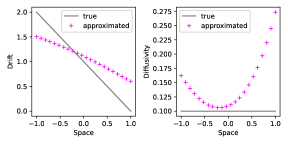
(a) The approximation results of SDE (6), (left) true and approximated drift coefficients, (right) true and approximated diffusivity coefficients

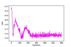
(b) Loss function

Figure 1: The estimated results of drift and diffusion coefficients, and corresponding loss. (a) Comparison of ground truth and approximation of drift and diffusion coefficients. (b) Loss over iterations shows training convergence.

It is shown in Figure 1 that even the training loss is decreasing and convergent, the approximation of drift and diffusion coefficients is still far from accurate. Therefore, log-likelihood function as a loss function is not enough for the identification of $\alpha$-stable Lévy noise driven stochastic differential equations. Now we present our framework in details in the next section for solving this issue.

3 Research framework

In this section, we investigate how to discover stochastic dynamics driven by $\alpha$-stable Lévy noise. Here we propose a deep learning algorithm to extract the stochastic differential equations as the form (1) from samples. It is important to note that our research focuses on both additive and multiplicative noise, without limited requirements on small noise intensity. Before introducing our methodology, we give the workflow of our constructed framework (Figure 2).

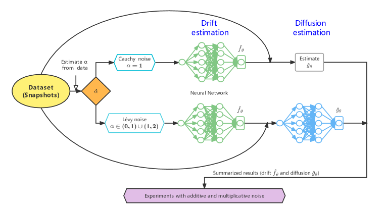
Figure 2: The workflow of our proposed framework. The estimation of stability parameter $\alpha$ is briefly introduced in Section 3.1. After determining whether it is Cauchy noise ($\alpha=1$), different structures are used to identify the dynamic behavior, see details in Section 3.3. Experiments with stochastic differential equations driven by additive or multiplicative noise are carried out in Section 4.

3.1 Estimation of stability parameter $\alpha$

In Section 2.1, we know that $\alpha$-stable random variables have stability parameter $\alpha$. The stability parameter estimation is not a new research topic and has been widely studied. Therefore, a couple of techniques have been investigated for stability parameter estimation, such as quantile method [McC86], characteristic function method [IH98], maximum likelihood method [Nol01], extreme value method, fractional lower order moment method [BMA10], method of log-cumulant [NA11], characteristic function based analytical approach [BAA17], Markov chain Monte Carlo with Metropolis-Hastings algorithm[HSSL11], moment generating function method [Nol13][LLXD21].

We attempt to estimate $\alpha$ using Markov chain Monte Carlo with Metropolis-Hastings algorithm and moment generating function method: when the stability parameter equals to 1.5, i.e., $\alpha=1.5$, Markov chain Monte Carlo with Metropolis-Hastings algorithm (MCMC with MH) shows that $\alpha$ converges to about $1.4930$ (Figure 3); and the result of direct calculation of the moment generating function is $1.5161$. Due to the validity of the above methods, the stability parameter $\alpha$ is assumed to be known in subsequent studies.

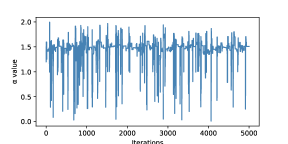
(a) Iteration results

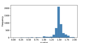
(b) Histogram of the $\alpha$ value frequency number

Figure 3: For the true $\alpha=1.5$, the iterative result of Markov chain Monte Carlo with Metropolis-Hastings algorithm (a) and a histogram of the $\alpha$ frequency number (b). Both iteration and histogram show that the $\alpha$ value is around $1.5$.

3.2 Challenge issues explanation

Here we continue to use the data structure mentioned in Section 2.2, i.e., a set of $N$ snapshots $D=\{(x_{1}^{(k)},x_{0}^{(k)},h^{(k)})\}_{k=1}^{N}$. Since we are thinking about autonomous systems, these samples can be viewed as starting at the same time in the state space and passing through the same time-step $h$, or they can be viewed as taking data pairs from a long trajectory $\{x_{t_{i}}\}$ of (1) with sample frequency $h_{i}>0$, that is, $t_{i+1}=t_{i}+h_{i}$. Note that, the step size $h^{(k)}$ is defined for each snapshot, so it may have different values for every index $k$ and every task. The main research is to discover drift $f$ and diffusion (diffusivity or noise intensity) $g$ through two neural networks $f_{\theta}:\mathbb{R}^{d}\rightarrow\mathbb{R}^{d}$ and $g_{\theta}:\mathbb{R}^{d}\rightarrow\mathbb{R}^{d}\times\mathbb{R}^{d}$, parameterized by their weights and bias $\theta$, only from the data in $D$. We restrict the discussion to the case $d=1$ for our main work in Section 3.3 and multi-dimensional cases could be explained and discussed in Section 3.4. Our initial idea is to utilize log-likelihood estimation to construct the loss function, that is, minimizing loss function implies maximization of the log-likelihood function. However, as can be seen at the end of Section 2.2, log-likelihood alone is not enough to serve as the loss function of neural networks, and we give the following explanation.

Log-likelihood function in a dilemma:

First, we discuss the problems encountered in the case of maximal likelihood estimation in the face of the Cauchy distribution, i.e., stable parameter $\alpha=1$. Maximum likelihood can also be used to estimate the location parameter $\gamma$ and the scale parameter $\sigma$ in Table 2. If a set of i.i.d. samples of size $N$ is taken from a Cauchy distribution ($S_{1}(\sigma,0,\gamma)$), the log-likelihood function is:

$$\mathcal{L}(z_{1},\dots,z_{N}|\sigma,\gamma)=\frac{1}{N}\sum_{k=1}^{N}p_{\alpha=1}(z_{k}|\sigma,\gamma)=-\log(\sigma\pi)-\frac{1}{N}\sum_{k=1}^{N}\log\Big{(}1+\Big{(}\frac{z_{k}-\gamma}{\sigma}\Big{)}^{2}\Big{)}.$$ (8)

Maximizing the log-likelihood function with respect to $\gamma$ and $\sigma$ by taking the first derivative produces the following system of equations:

$$\begin{split}\frac{d\mathcal{L}}{d\gamma}&=\sum_{k=1}^{N}\frac{2(z_{k}-\gamma)}{\sigma^{2}+(z_{k}-\gamma)^{2}}=0,\\ \frac{d\mathcal{L}}{d\sigma}&=\sum_{k=1}^{N}\frac{2(z_{k}-\gamma)^{2}}{\sigma(\sigma^{2}+(z_{k}-\gamma)^{2})}-\frac{N}{\sigma}=0.\end{split}$$ (9)

We can see that solving $\gamma$ requires handling a polynomial of degree $2n-1$, and solving $\sigma$ requires computing a polynomial of degree $2n$. This tends to be complicated by the fact that this requires finding the roots of a high degree polynomial, and there can be multiple roots that represent local maximum [Fer78]. In [Zha91], the authors give a counterexample that the likelihood equation has multiple roots and the maximum likelihood estimator may not be unique. They also show that the maximum likelihood estimator can only be approximated by numerical methods which makes it very inconvenient to apply the usual maximum likelihood estimator method to Cauchy distribution. Meanwhile, because the expectation and variance of Cauchy distribution don’t exist, the usual moment estimation method is not suitable for the parameter estimation of Cauchy distribution.

Then, since the general $\alpha$-stable distribution doesn’t have a closed-form of its probability density function (Appendix A), it’s natural to wonder the rationality of the maximum log-likelihood function as a loss function. We follow the initial loss function and construction in Section 2.2, that is, only the negative log-likelihood function is used as the loss function. An experiment of SDE (6) with training results of neural networks is shown in the Figure 1.

Unsurprisingly, as discussed in the Cauchy noise case, the results of simply using the log-likelihood function as a loss are poor. We give the following explanations: the probability density functions of $\alpha$-stable distributions are too complex, the maximum likelihood estimation falls into local extremes; estimating two unknown quantities with a function is inherently uncertain. On the other hand, we cannot completely negate the log-likelihood function as a loss function. Looking at Figure 1, it can be found that the estimated results of the drift coefficient $f_{\theta}$ and the diffusion coefficient $g_{\theta}$ are better and worse at the same time. Intuitively, the maximum likelihood estimator needs an auxiliary method to determine its value to prevent the optimization process of the maximum likelihood estimator from falling into local minimums.

To sum up, the log-likelihood function is not a panacea. Constructing the loss function solely by maximizing likelihood function is sufficient for the Brownian noise case and small noise, but not for $\alpha$-stable Lévy noise case. We will discuss how to build neural networks and loss functions in different stability parameter scenarios.

3.3 Two-step hybrid method (1-D)

In previous section, we see problems with log-likelihood functions for $\alpha$-stable Lévy case, hence here we explore the solutions through a two-step learning framework.

3.3.1 A special case — Cauchy

Let us begin with the special case of identifying stochastic dynamical systems with Cauchy noise ($\alpha=1$).

Inspired by [Wan21], the least absolutely deviation(LAD) estimation is advocated by Laplace which has the advantage of robustness. The introduction of the robustness requirement is one of the major advances in statistics in the second half of the 20th century. By definition, the least absolutely deviation estimate is the value $\gamma$ that minimizes the mean absolute deviation:

$$H(\gamma)=\sum_{k=1}^{N}|z_{k}-\gamma|,$$ (10)

where $(z_{1},z_{2},...,z_{N})$ represent the $N$ i.i.d. samples of Cauchy distribution with parameters $\gamma$ and $\sigma$. If we find the least absolutely deviation of the parameter $\gamma$, denoted as $\hat{\gamma}_{N}$, the parameter $\sigma$ can be estimated as follows:

$$\hat{\sigma}_{N}=\frac{1}{2}\Big{[}\frac{1}{N}\sum_{k=1}^{N}\sqrt{|z_{k}-\hat{\gamma}_{N}|}\Big{]}^{2}.$$ (11)

Note that $\hat{\sigma}_{N}$ is calculated directly by the formula (11). Moreover, the parameters $\hat{\gamma}_{N}$ and $\hat{\sigma}_{N}$ obtained by the above method are strong consistency estimator, i.e., $\hat{\gamma}_{N}$ and $\hat{\sigma}_{N}$ converge to $\gamma$ and $\sigma$ with probability 1. Thus, we propose our learning schemes in the following two steps.

Step 1: Corresponding to our task, for the drift coefficient $f_{\theta}$, we construct a loss function similar to (10):

$$\begin{split}\mathcal{L}(\theta|x_{1},x_{0},h)=\sum_{k=1}^{N}|x_{1}^{(k)}-(x_{0}^{(k)}+hf_{\theta}(x_{0}^{(k)}))|.\end{split}$$ (12)

By minimizing the loss function (12), we obtained the drift item $\hat{f}_{\theta}$ we expected.

Step 2: As for the diffusion coefficient $g_{\theta}$, it can be obtained by direct calculation of the analog of formula (11):

$$\hat{g}_{\theta}(x_{0}^{(i)})=\frac{1}{2}\Big{[}\frac{1}{N_{i}}\sum_{k_{i}=1}^{N_{i}}\sqrt{|x_{1}^{(k_{i})}-(x_{0}^{(i)}+h\hat{f}_{\theta}(x_{0}^{(i)}))|}\Big{]}^{2},\ for\ i=1,2,\dots,n,$$ (13)

where $N_{1}+N_{2}+\dots+N_{n}=N$.

3.3.2 General cases when $\alpha\in(0,2)\setminus\{1\}$

In this section, we will find that the log-likelihood function plays a key role in training. Since it contains the probability density function, we will first introduce the probability density function of the $\alpha$-stable random variable we used.

Although there are three probability density functions available (Appendix A.1), as they all contain integrals or infinite series, it is difficult to maximize the log-likelihood function. After programming experiments, Zolotarev formula is the most stable and accurate one. However, because of the truncation error from approximated summation, other two functions cannot give us appropriate approximations when state space is wide and density is comparatively smooth.

Zolotarev formula: The probability density function of $X\sim S_{\alpha}(1,0,0)$ is:

$$p(x;\alpha,\beta=0,\sigma=1,\gamma=0)=\left\{\begin{array}[]{lr}\dfrac{\alpha x^{\frac{1}{\alpha-1}}}{\pi|\alpha-1|}\int_{0}^{\frac{\pi}{2}}V(\theta;\alpha,\beta=0)\exp\{-x^{\frac{1}{\alpha-1}}V(\theta;\alpha,\beta=0)\}d\theta,\ for\ x>0,\\ \\ \dfrac{\Gamma(1+\frac{1}{\alpha})}{\pi},\ for\ x=0,\\ \\ p(-x;\alpha,-\beta=0,\sigma=1,\gamma=0),\ for\ x<0,\\ \end{array}\right.$$ (14)

where $V(\theta;\alpha,\beta=0)=\Big{(}\dfrac{\cos\theta}{\sin\alpha\theta}\Big{)}^{\frac{\alpha}{\alpha-1}}\cdot\dfrac{\cos\{(\alpha-1)\theta\}}{\cos\theta}$. A description of other forms of probability density functions is in the Appendix A.1. Unless otherwise specified, the $\alpha$-stable probability density function we generally use is the Zolotarev formula (14, A3). We introduce a proposition that has important implications for subsequent derivations:

Proposition 1.

(i) If $X\sim S_{\alpha}(\sigma,\beta,\gamma)$ and $a$ is a real constant, then $X+a\sim S_{\alpha}(\sigma,\beta,\gamma+a)$.
(ii) If $X\sim S_{\alpha}(\sigma,\beta,\gamma)$ and $k$ is a real constant, then

$$kX\sim\left\{\begin{array}[]{lr}S_{\alpha}(|k|\sigma,\mathrm{sgn}(k)\beta,k\gamma),\ \alpha\neq 1,\\ \\ S_{1}(|k|\sigma,\mathrm{sgn}(k)\beta,k\gamma-\frac{2}{\pi}k(\log|k|)\sigma\beta),\ \alpha=1.\\ \end{array}\right.$$ (15)

In particular, if $X\sim S_{\alpha}(1,0,0)$ and $k$ is a real constant, then $kX\sim S_{\alpha}(|k|,0,0)$, for $\alpha\in(0,2)$.
(iii) If $X\sim S_{\alpha}(\sigma,\beta,0)$, then $-X\sim S_{\alpha}(\sigma,-\beta,0)$, for $\alpha\in(0,2)$.
(iv) If $X_{1}$, $X_{2}$ are independent stable random variables with the same distribution $S_{\alpha}(\sigma,\beta,\gamma)$ for $\alpha\neq 1$ and $A$, $B$ are positive constants, then

$$AX_{1}+BX_{2}\sim S_{\alpha}(\sigma(A^{\alpha}+B^{\alpha})^{\frac{1}{\alpha}},\beta,\gamma(A+B)).$$

Proof.

See [ST95], Chapter 1. ∎

Hence, if $p_{\alpha}(x;\sigma,\beta,\gamma)$ is the probability density function of the stable random variable $X\sim S_{\alpha}(\sigma,\beta,\gamma)$, then $p_{\alpha}(x;\sigma,\beta,\gamma+a)$ is the probability density function of $X+a$ (for every real constant $a$) and $p_{\alpha}(x;\sigma A,\beta,\gamma A)$ is the probability density function of $AX$ (for every positive constant $A$ and $\alpha\neq 1$).

Similar to the Gaussian noise, it also starts from Euler-Maruyama discretization method (2) for training the networks $f_{\theta}$ and $g_{\theta}$. Essentially, conditioned on $x_{0}$ and $h$, we can think of $x_{1}$ as a point extracted from a $\alpha$-stable distribution:

$$x_{1}\sim S_{\alpha}(g(x_{0})h^{1/\alpha},0,x_{0}+hf(x_{0})),$$ (16)

where we use the argument (i) and (ii) in Proposition 1 and the fact $L^{\alpha}_{h}\sim S_{\alpha}(h^{\frac{1}{\alpha}},0,0)$. As mentioned in Zolotarev fomula (14, A3), we introduce the probability density function of $X\sim S_{\alpha}(1,0,0),\ \alpha\in(0,2)\setminus\{1\}$. In order to get the probability density function of (16), we need a simple derivation.

Remark 1.

If $X\sim S_{\alpha}(1,0,0)$ has probability density function $p_{\alpha}(x)$, $b$, $A>0$ are constants, then $b+AX\sim S_{\alpha}(A,0,b)$ has the probability density function $\frac{1}{A}p_{\alpha}(\frac{x-b}{A})$. This comes from the fact that $\mathbb{P}(b+AX\leq x)=\mathbb{P}(X\leq\frac{x-b}{A})=\int_{-\infty}^{\frac{x-b}{A}}p_{\alpha}(\xi)d\xi$ and $\frac{d}{dx}\mathbb{P}(b+AX\leq x)=\frac{1}{A}p_{\alpha}(\frac{x-b}{A})$.

After preparing the required probability density function and its transformation formula, we first need to construct an auxiliary measure for the log-likelihood function. In our method, it manifests as the first step in the two-step estimation method, i.e., estimating drift coefficient $f$.

Step 1: Observation of the $x_{1}$ distribution (16) shows that the drift coefficient $f$ is essentially related to the location parameter of the $\alpha$-stable random variable. Taking inspiration from improvements to Cauchy estimation, we choose to first estimate the drift $f$ or the location parameter of $x_{1}$ distribution using a neural network. From a machine learning perspective, the estimation of the Cauchy drift coefficient $f_{\theta}$ can essentially be considered as Mean Absolute Error (MAE). After testing, we find that the Mean square Loss (MSE) converges faster than MAE and the results are better. For the drift neural network $f_{\theta}$, we use the following loss function:

$$\mathcal{L}(\theta|x_{1},x_{0},h)=\frac{1}{N}\sum_{k=1}^{N}[x_{1}^{(k)}-(x_{0}^{(k)}+hf_{\theta}(x_{0}^{(k)}))]^{2}.$$ (17)

Minimizing the above loss function (17), we obtain the desirable drift estimation $\hat{f}_{\theta}$.

Step 2: Since the estimation of the drift $\hat{f}_{\theta}$ assists the log-likelihood function, we can now formulate the log-likelihood loss function that will be minimized to obtain the neural network weights $\theta$ for diffusion network $g_{\theta}$. The log-likelihood formula of the data set $D$ is no change in form (4) except the notion $p_{\theta}$ means the probability density function of (16). If we bring in the probability density function (14) and apply the conclusion from Remark 1, we can get a loss function of the analogous form (5). We note that the specific form (3) and (16) of the transition probabilities $p_{\theta}$ induced by the Euler-Maruyama method implies that it is only the conditional probability given $x_{0}$ and $h$. So we need data pairs such as $(x_{0},x_{1})$, and the conclusion that the conditional distribution of $x_{1}$ after multi-step evolution is still a $\alpha$-stable distribution is often wrong.

The logarithm of the probability density function of the $\alpha$-stable distribution, together with four parameters from (16), yields the loss function to minimize, that is,

$$\begin{split}\mathcal{L}(\theta|x_{1},x_{0},h):&=-\frac{1}{N}\sum_{k=1}^{N}\log p_{\theta}(x_{1}^{(k)}|x_{0}^{(k)},h)\\ &=-\frac{1}{N}\sum_{k=1}^{N}\log\Big{[}\frac{1}{g_{\theta}(x_{0}^{(k)})h^{1/\alpha}}p_{\alpha}\Big{(}\frac{x_{1}^{(k)}-(x_{0}^{(k)}+hf_{\theta}(x_{0}^{(k)}))}{g_{\theta}(x_{0}^{(k)})h^{1/\alpha}}\Big{)}\Big{]}\\ &=\frac{1}{N}\sum_{k=1}^{N}\log(g_{\theta}(x_{0}^{(k)})h^{1/\alpha})-\frac{1}{N}\sum_{k=1}^{N}\log\Big{[}p_{\alpha}\Big{(}\frac{x_{1}^{(k)}-(x_{0}^{(k)}+hf_{\theta}(x_{0}^{(k)}))}{g_{\theta}(x_{0}^{(k)})h^{1/\alpha}}\Big{)}\Big{]}\end{split}$$ (18)

where $p_{\alpha}$ represents the probability density function of the $\alpha$-stable random variable $S_{\alpha}(1,0,0)$. Minimizing $\mathcal{L}$ in (18) over the data $D$ is equivalent to maximization of the log-likelihood function (4).

Using the estimated drift coefficient $\hat{f}_{\theta}$, bring in to (18) and minimize, we can get the desired diffusion estimation $\hat{g}_{\theta}$. Such a two-step training method avoids weight adjustment between loss functions on the one hand and gives the log-likelihood function an auxiliary estimation on the other hand.

3.4 Multi-dimensional case

We continue with the setting in Section 2.1, i.e., diffusion coefficient $g(X_{t})$ is a $d\times d$ diagonal matrix and the $d$-dimensional $\alpha$-stable Lévy motion is composed of $d$ mutually independent one-dimensional symmetric $\alpha$-stable Lévy motions. Based on these assumptions, we can generalize our algorithm to multi-dimensional stochastic differential equations.

Step 1: Compared to Step 1 of Section 3.3.2, we rewrite the loss function (17) to the average of $d$ dimensions:

$$\mathcal{L}(\theta|x_{1},x_{0},h)=\frac{1}{Nd}\sum_{k=1}^{N}\sum_{i=1}^{d}[x_{1,i}^{(k)}-(x_{0,i}^{(k)}+hf_{\theta,i}(x_{0}^{(k)}))]^{2}.$$ (19)

where $x_{j}=(x_{j,1},x_{j,2},\dots,x_{j,d})^{T}$ for $j=0,1$ and $f_{\theta}(x_{0})=(f_{\theta,1}(x_{0}),f_{\theta,2}(x_{0}),\dots,f_{\theta,d}(x_{0}))^{T}$ are $d$-dimensional vectors, time step $h$ is a scalar value.

Step 2: After getting the estimated drift coefficient $\hat{f}_{\theta}$, the diffusion coefficient $g$ is the only thing left to figure out. Since $g$ is a diagonal matrix and the components of Lévy motion are mutually independent, under conditional probability, we can write the joint distribution as the product of marginal distributions:

$$p(x_{1}|x_{0},h,f(x_{0}))=p(x_{1,1}|x_{0},h,f(x_{0}))p(x_{1,2}|x_{0},h,f(x_{0}))\dots p(x_{1,d}|x_{0},h,f(x_{0})),$$ (20)

where $x_{1}$, $x_{0}$ and $f(x_{0})$ are $d$-dimensional vectors, time step $h$ is a scalar value. Take the logarithm of the equation (20):

$$\log p(x_{1}|x_{0},h,f(x_{0}))=\sum_{i=1}^{d}\log p(x_{1,i}|x_{0},h,f(x_{0})).$$ (21)

Furthermore, we can briefly rewrite the formula (18):

$$\mathcal{L}(\theta|x_{1},x_{0},h,\hat{f}_{\theta}(x_{0}))=-\frac{1}{N}\sum_{k=1}^{N}\sum_{i=1}^{d}\log p_{\theta}(x_{1,i}^{(k)}|x_{0}^{(k)},h,\hat{f}_{\theta}(x_{0}^{(k)})).$$ (22)

The required diffusion coefficient $g$ is estimated by $\hat{g}_{\theta}$ through minimizing the formula (22).

Note that this generalization of $d$-dimensional SDEs is because the $d$-dimensional probability density function that can be written as the product of one-dimensional marginal density functions (20). Further, we can explain assumptions that $g(X_{t})$ is a diagonal matrix and that the components of Lévy motion are mutually independent in Section 2.1. Without the assumption that $g(X_{t})$ is a diagonal matrix, we consider a two-dimensional SDE and use the Euler-Maruyama scheme (2) represented as follows:

$$X_{1} =X_{0}+hf_{1}(X_{0},Y_{0})+A_{1}L_{h,1}^{\alpha}+A_{2}L_{h,2}^{\alpha},$$ (23)

$$Y_{1} =Y_{0}+hf_{2}(X_{0},Y_{0})+B_{1}L_{h,1}^{\alpha}+B_{2}L_{h,2}^{\alpha},$$

where constants $A_{1},A_{2},B_{1},B_{2}>0$ and $L_{h,1}^{\alpha},L_{h,2}^{\alpha}$ are independent and $\alpha$-stable distributed. Although the linear combination of independent $\alpha$-stable random variables is still an $\alpha$-stable random variable (Proposition 1, (iv)), $X_{1}$ and $Y_{1}$ aren’t independent, and the joint distribution of the random vector $(X_{1},Y_{1})^{T}$ cannot be expressed as the product of marginal distributions. Without the assumption that the components of Lévy motion are mutually independent, the explicit probability density function of this two-dimensional random vector $(X_{1},Y_{1})^{T}$ is unknown. Besides that, we introduce another case of $d$-dimensional $\alpha$-stable random vectors. In [Nol13], the author discussed the $d$-dimensional elliptically contoured $\alpha$-stable distribution whose probability density function can be computed through amplitude distribution and surface integral. However, its complicated probability density function leads to intractable approximations, which is beyond the scope of our article.

4 Experiments

We illustrate the neural network identification techniques in the following examples, divided by different ranges of $\alpha$ value ($\alpha=1$, $\alpha\in(1,2)$, $\alpha\in(0,1)$), the categories of noise (additive noise or multiplicative noise) and the dimensions of SDEs. We created snapshots by integrating the SDEs (1) from $t=0$ to $t=h$. To be specific, these samples come from simulating stochastic differential equation with initial value $x_{0}$ using Euler-Maruyama scheme, where $x_{0}\in[-3,3]$, $x_{0}\in[-1,1]$, $x_{0}\in[-2.5,2.5]$ for different examples.

In this article, we consider stochastic dynamical systems induced by medium noise or large noise, and noise very close to 0 is not considered (noise very close to 0 can be approximated as a deterministic system). Furthermore, we use a Softplus activation function before output $g_{\theta}$, to guarantee $g_{\theta}$ is always positive. In addition, we clipped the lower bound of output $g_{\theta}$ with $10^{-13}$, so that we won’t have loss go to infinity.

To avoid confusion, we post a list of experiments in Table 1. Since the drift coefficients and diffusion coefficients learned by the neural network are implicitly expressed, and the negative log-likelihood function is not necessarily greater than $0$ as the general loss function, we calculate the $\mathcal{L}^{2}$ error of the two coefficients in addition to the figures to explicitly quantify the experimental results:

$$\mathcal{L}_{f}^{2}=\frac{1}{N}\sum_{k=1}^{N}(f(x_{0}^{(k)})-\hat{f}_{\theta}(x_{0}^{(k)}))^{2},\ \mathcal{L}_{g}^{2}=\frac{1}{N}\sum_{k=1}^{N}(g(x_{0}^{(k)})-\hat{g}_{\theta}(x_{0}^{(k)}))^{2}.$$ (24)

The results can be seen in the last two columns of Table 1.

Table 1: List of experiments (Experiments with font bolding can be found in this section and the remaining experiments are shown in Appendix C)

Stability	Noise type	Drift	Diffusion	Error	Error
parameter		coefficient $f$	coefficient $g$	$\mathcal{L}^{2}_{f}$	$\mathcal{L}^{2}_{g}$
$\alpha=1$	additive	$-X_{t}+1$	$1$	0.0021	0.0004
		$\bm{-X_{t}^{2}}$	$\bm{1}$	0.0020	0.0000
		$\sin(X_{t})$	$1$	0.0080	0.0017
	multiplicative	$-X_{t}+1$	$0.1X_{t}+0.5$	0.0041	0.0147
		$\bm{-X_{t}^{2}}$	$\bm{0.1X_{t}+0.5}$	0.0344	0.0136
		$\sin(X_{t})$	$0.1X_{t}+0.5$	0.0054	0.0173
$\alpha=1.5$	additive	$-X_{t}+1$	$1$	0.0038	0.0007
		$-X_{t}^{3}+X_{t}$	$1$	0.0010	0.0003
		$\log(X_{t}+1.5)$	$1$	0.0003	0.0008
		$-|X_{t}+1.5|^{1/3}$
	multiplicative	$\bm{-X_{t}^{3}+X_{t}}$	$\bm{X_{t}+1}$	0.0009	0.0007
		$\bm{-X_{t}^{3}+X_{t}}$	$\bm{\sin(\pi X_{t})+1}$	0.0006	0.0108
$\alpha=0.5$	additive	$-X_{t}+1$	$1$	0.0001	0.0045
		$-X_{t}^{3}+X_{t}$	$1$	0.0002	0.0010
	multiplicative	$-X_{t}+1$	$X_{t}+1$	0.0001	0.0139
		$-X_{t}^{3}+X_{t}$	$X_{t}+1$	0.0002	0.0047
compared with nonlocal	additive	$\bm{-X_{t}^{3}+4X_{t}}$	$\bm{1}$	0.0014	0.0003
Kramers-Moyal
(2-D) $\alpha=1.5$	additive	$\bm{X_{t}-X_{t}^{3}-X_{t}Y_{t}^{2}}$	$\bm{1}$	0.0014	0.0026
		$\bm{-(1+X_{t}^{2})Y_{t}}$	$\bm{1}$
	multiplicative	$X_{t}+Y_{t}$	$0.5Y_{t}+1$	0.0024	0.0020
		$4X_{t}-2Y_{t}$	$0.5X_{t}+1$

4.1 SDEs driven by Cauchy motion

In this section, we test the special case of $\alpha=1$. The drift neural networks $f_{\theta}$ in our tests have two hidden layers and 25 neurons per layer, batch size of 100, 100 epochs, with exponential linear unit (ELU) activation function and the ADAMAX optimizer with default parameters. The diffusion coefficients $g_{\theta}$ are calculated by formula (13).

We present two representative examples in this section: (1) additive noise, i.e., $g(X_{t})$ in (1) is a constant, we assume $g(X_{t})=1$ without loss of generality; (2) multiplicative noise with a diffusion coefficient of $g(X_{t})=0.1X_{t}+0.5$. Both drift coefficients are $f(X_{t})=-X_{t}^{2}$. Here we take sample size $N=10000$, $h=0.01$, $x_{0}\in[-3,3]$ for example (1). Example (2) follows the construction of example (1) except for sample size $N=20$ (different $x_{0}$) $\times 1000$ (sample size). By comparing the real coefficients with the learned coefficients in Figure 4, we can see that they overlap very well.

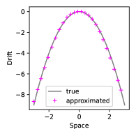
(a) $f(X_{t})=-X_{t}^{2}$, $\hat{g}_{\theta}=0.9955$

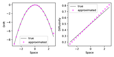
(b) $f(X_{t})=-X_{t}^{2}$, $g(X_{t})=0.1X_{t}+0.5$, (left) true and approximated drift coefficients, (right) true and approximated diffusivity coefficients

Figure 4: Cauchy noise with two representative examples, the gray lines represent the true coefficients and the magenta plus markers are the neural networks’ results. $\hat{g}_{\theta}$ represents the diffusion coefficient calculated by (13).

4.2 SDEs driven by $\alpha$-stable Lévy motion

In this section, neural networks are used twice, separately to estimate drift and diffusion. The drift neural networks $f_{\theta}$ have three hidden layers and 25 neurons per layer, no batch normalization, 300 epochs, with exponential linear unit (ELU) activation function, and the ADAM optimizer with a learning rate of $0.005$ and other default parameters. The diffusion neural networks $g_{\theta}$ have two hidden layers and 25 neurons per layer, output layer with the Softplus function to ensure that the diffusion coefficients are positive, batch size of 512, no more than $30$ epochs, with exponential linear unit (ELU) activation function and the ADAMAX optimizer with a learning rate of $0.005$, eps $=10^{-7}$ and other default parameters.

We separately discuss $\alpha\in(1,2)$ and $\alpha\in(0,1)$. This is due to the fact that as $\alpha$ decreases, the probability distribution function presents a greater probability near the location parameter and a greater probability of the tail, which results in a difference in the accuracy of the estimated result. Without loss of generality, we select $\alpha=1.5$ and $\alpha=0.5$.

As described in Table 1 and Appendix C, our experiments on drift $f$ focus on linear drift coefficients, double-well drift coefficients, and complex drift coefficients. Additive noise remains $g=1$. Multiplicative noise contains linear diffusion coefficients and trigonometric diffusion coefficients. We use a preprocessing trick to speed up training and improve estimation accuracy, see Appendix B. Different experimental parameters may vary slightly. We give an appropriate explanation for different step sizes. Indeed, take a glance at the loss function (17), our goal is to find the optimal $f_{\theta}$ but it is affected by the step size, and too small a step size can make it difficult to estimate $f$. On the other hand, too large a time step can cause the precision of the Euler-Maruyama scheme to decrease. Therefore, there is a trade-off between them. For a smaller time step, bringing more samples into the training process is one way to achieve the same estimated precision.

We look at representative examples once more and provide suggestions for improvement. For $\mathbf{\alpha=1.5}$, we test the drift coefficients $f(X_{t})=-X_{t}^{3}+X_{t}$, diffusion coefficient $g(X_{t})=X_{t}+1$ and $g(X_{t})=\sin(\pi X_{t})+1$ in equation (1). Here we take sample size $N=50\times 1000$, $h=0.5$, $x_{0}\in[-1,1]$. We compare the true coefficients and the learned coefficients in Figure 5.

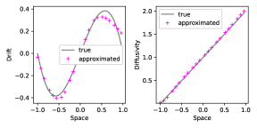
(a) $f(X_{t})=-X_{t}^{3}+X_{t}$, $g(X_{t})=X_{t}+1$, (left) true and approximated drift coefficients, (right) true and approximated diffusivity coefficients

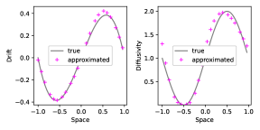
(b) $f(X_{t})=-X_{t}^{3}+X_{t}$, $g(X_{t})=\sin(\pi X_{t})+1$, (left) true and approximated drift coefficients, (right) true and approximated diffusivity coefficients

Figure 5: Multiplicative noise with different diffusion coefficients for $\alpha=1.5$, the gray lines represent the true coefficients and the magenta plus markers are the estimated drift and diffusion results from our proposed neural networks.

Improvement of accuracy:

A cursory look reveals that the estimation results are poor when the noise is large, i.e., the poor performance at the right end of the axis of Figure 5. We add more samples at the large noise, and the data volume becomes $75\times 1000$ which the extra samples are added to the interval $(0,1)$. The improved results are shown in Figure 6.

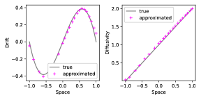
(a) $f(X_{t})=-X_{t}^{3}+X_{t}$, $g(X_{t})=X_{t}+1$, (left) true and approximated drift coefficients, (right) true and approximated diffusivity coefficients

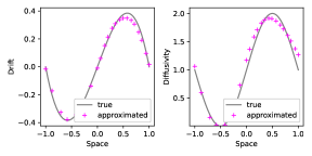
(b) $f(X_{t})=-X_{t}^{3}+X_{t}$, $g(X_{t})=\sin(\pi X_{t})+1$, (left) true and approximated drift coefficients, (right) true and approximated diffusivity coefficients

Figure 6: Multiplicative noise with different diffusion coefficients for $\alpha=1.5$, increased sample size at large noise, the gray lines represent the true coefficients and the magenta plus markers are the estimated drift and diffusion results from our proposed neural networks.

4.3 Comparison with nonlocal Kramers-Moyal formulas

Next, we compare a novel method mentioned in [LLXD21] which stability parameter $\alpha\in(1,2)$ (due to limitations of the moment generation function method). In this paper, they approximate the stability parameter $\alpha$ and noise intensity $g$ through computing the mean and variance of the amplitude of increment of the sample paths. Then they estimate the drift coefficient via nonlocal Kramers-Moyal formulas. We keep settings consistent, i.e., $N=50\times 1000$, $x_{0}\in[-2.5,2.5]$, the true drift coefficient $f(X_{t})=4X_{t}-X_{t}^{3}$ and the constant noise term $g=1$ except step size. For more details, see [LLXD21]. Figure 7 shows the results of the comparison, the results are comparable and our work is somewhat competitive.

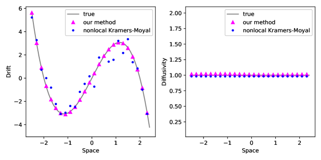
Figure 7: Compare with nonlocal Kramers-Moyal formulas with moment generation function by a data-driven method, the gray lines represent the true coefficients, the magenta triangle markers are our results and the blue dots are results of nonlocal Kramers-Moyal method with moment generation function, (left) true and approximated drift coefficients, (right) true and approximated diffusivity coefficients

4.4 Multi-dimensional experiments

Finally, we implement the multi-dimensional situation stated in Section 3.4. The neural networks are built in the same way that Section 4.2 is. Consider the Maier-Stein model under $\alpha$-stable Lévy noise in $\mathbb{R}^{2}$:

$$dX_{t} =(X_{t}-X_{t}^{3}-kX_{t}Y_{t}^{2})dt+dL_{t,1}^{\alpha},$$ (25)

$$dY_{t} =[-(1+X_{t}^{2})Y_{t}]dt+dL_{t,2}^{\alpha},$$

where $L_{t,1}^{\alpha}$, $L_{t,2}^{\alpha}$ are two independent one-dimensional symmetric $\alpha$-stable Lévy motions and $k$ is a positive parameter. We assign $k$ to $1$, as detailed in [LDLZ20]. Since we have a different structure of the multi-dimensional Lévy motion, we no longer compare our methods with those in [LLXD21]. We take sample size $N=(40\ \text{different values of}\ x_{0},\ y_{0}\ \text{respectively})\times 1000$, $h=0.5$, $(x_{0},y_{0})\in[-1,1]\times[-1,1]$ and $\alpha=1.5$. We compare the true coefficients and the learned coefficients in the form of heat maps (Figure 8). Intuitively, the method we proposed reaches a relatively good estimation, and $\mathcal{L}^{2}$ errors support this view.

Moreover, we give a simple linearly coupled two-dimensional SDE with multiplicative noise in Appendix C.3 as a validation for multi-dimension with multiplicative noise. However, with the dimension of the state space increasing, the sample size needs to grow dramatically, causing issues such as high computational burden and memory limit exceeded. This inspires us to look for more innovative algorithms with sample efficiency and relatively lower computational cost.

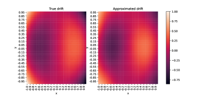
(a) $f_{1}(X_{t},Y_{t})=X_{t}-X_{t}^{3}-X_{t}Y_{t}^{2}$, (left) true drift coefficient, (right) approximated drift coefficient

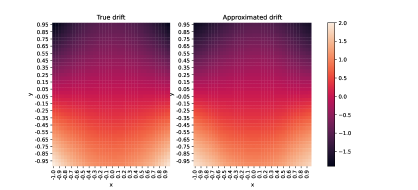
(b) $f_{2}(X_{t},Y_{t})=-(1+X_{t}^{2})Y_{t}$, (left) true drift coefficient, (right) approximated drift coefficient

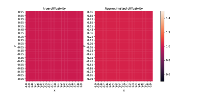
(c) $g_{1}(X_{t},Y_{t})=1$, (left) true diffusivity coefficient, (right) approximated diffusivity coefficient

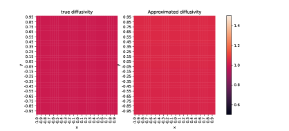
(d) $g_{2}(X_{t},Y_{t})=1$, (left) true diffusivity coefficient, (right) approximated diffusivity coefficient

Figure 8: The drift coefficients (true and estimated) and diffusion coefficients (true and estimated) of the Maier-Stein model, presented as heat maps.

5 Summary

In this article, we have devised a novel method based on neural networks to identify stochastic dynamics from snapshot data. In particular, we start with a simple identification of the stability parameter and then estimate the drift coefficient via the network. After obtaining an estimation of the drift coefficient, we calculate the diffusion coefficient directly for Cauchy noise and estimate it through another neural network with log-likelihood estimation for $\alpha$-stable Lévy noise. Numerical experiments on both additive and multiplicative noise illustrate the accuracy and effectiveness of our method.

Compared with nonlocal Kramers-Moyal method with moment generation function, this method has the advantage that it doesn’t restrict the value range of the stability parameter and allow multiplicative noise. Even in the face of large noise, simply increasing the local sample size can improve the estimation.

Moreover, we use Maier-Stein model as an illustration for multi-dimensional SDEs under both additive and multiplicative Lévy noise.

We give some brief error analysis, and the error of this method is mainly derived from the following parts: errors from neural networks, maximum likelihood estimation, and discretization method. The first two types of errors can be thought as optimization error and generalization error which are determined by the model adopted and the sample size. The choice of hyperparameters also tends to be subjective through personal experience. The last error which can be regarded as approximation error depends on the numerical discretization method and replacing the numerical method also results in a change in the probability distribution, the likelihood function, and other details. We have tried to balance the various errors so that the result is what we want.

Finally, there still exist some limitations on the applications of this method. For example, although the maximum log-likelihood estimation is precise, the training process is slow. In addition, We will try to learn the probability density function in more general multi-dimensional cases.

Data Availability

The data that support the findings of this study are openly available in GitHub https://github.com/Fangransto/learn-alpha-stable-levy.git.

Appendix A The $\alpha$-stable random variables (1-D)

The $\alpha$-stable distributions are a rich class of probability distributions that allow skewness and heavy tails and have many intriguing mathematical properties. According to definition [Dua15], a random variable $X$ is called a stable random variable if it is a limit in distribution of a scaled sequence $(S_{n}-b_{n})/a_{n}$, where $S_{n}=X_{1}+\dots+X_{n}$, $X_{i}$ are some independent identically distributed random variables and $a_{n}>0$ and $b_{n}$ are some real sequences.

The distribution of a stable random variable is denoted as $S_{\alpha}(\sigma,\beta,\gamma)$. The $\alpha$-stable distribution requires four parameters for complete description: an index of stability $\alpha\in(0,2]$ also called the tail index, tail exponent or characteristic exponent, a skewness parameter $\beta\in[-1,1]$, a scale parameter $\sigma>0$ and a location parameter $\gamma\in\mathbb{R}^{1}$. As mentioned in [Dua15], [BHW05], [McC86] and [MDC⁺99], the $\alpha$-stable random variables $X\sim S_{\alpha}(\sigma,\beta,\gamma)$ whose densities lack closed form formulas for all but three distributions, see Table 2.

Table 2: Closed form formulas for three distributions.

Name	Parameters	Probability density function
normal distribution	$\alpha=2,\ \beta=0$	$p(x)=\dfrac{1}{\sqrt{(2\pi)\times(2\sigma^{2})}}\exp(-\dfrac{(x-\gamma)^{2}}{4\sigma^{2}})$
Cauchy distribution	$\alpha=1,\ \beta=0$	$p(x)=\dfrac{\sigma}{\pi[(x-\gamma)^{2}+\sigma^{2}]}$
Lévy distribution	$\alpha=1/2,\ \beta=1$	$p(x)=\left\{\begin{array}[]{lr}\sqrt{\dfrac{\sigma}{2\pi}}(x-\gamma)^{-\frac{3}{2}}\exp\big{[}-\dfrac{\sigma}{2(x-\gamma)}\big{]},\ for\ x>\gamma\\ \\ 0,\ for\ x\leq\gamma\\ \end{array}\right.$

A.1 Probability density functions and characteristic functions

Here we use three explicit expressions to express the probability density functions of standard symmetric $\alpha$-stable random variables ($X\sim S_{\alpha}(1,0,0)$, $\alpha\in(0,2)$, $\alpha\neq 1$):

• Represented as infinite series [Dua15],

  $$p(x;\alpha,\beta=0,\sigma=1,\gamma=0)=\left\{\begin{array}[]{lr}\frac{1}{\pi x}\sum_{k=1}^{\infty}\frac{(-1)^{k-1}}{k!}\Gamma(\alpha k+1)|x|^{-\alpha k}\sin(\frac{k\alpha\pi}{2}),\ for\ x\neq 0,\ 0<\alpha<1,\\ \\ \frac{1}{\pi}\int_{0}^{\infty}e^{-u^{\alpha}}du,\ for\ x=0,\ 0<\alpha<1,\\ \\ \frac{1}{\pi\alpha}\sum_{k=0}^{\infty}\frac{(-1)^{k}}{2k!}\Gamma(\frac{2k+1}{\alpha})x^{2k},\ for\ 1<\alpha<2.\\ \end{array}\right.$$ (A1)

• By virtue of characteristic functions and the Fourier transform [BHW05],

  $$p(x;\alpha,\beta=0,\sigma=1,\gamma=0)=\frac{1}{2\pi}\int_{-\infty}^{\infty}e^{-ixt}{\varphi(t;\alpha,\beta=0,\sigma=1,\gamma=0)}dt,$$ (A2)

• Zolotarev formulas [BHW05],

  $$p(x;\alpha,\beta=0,\sigma=1,\gamma=0)=\left\{\begin{array}[]{lr}\dfrac{\alpha x^{\frac{1}{\alpha-1}}}{\pi|\alpha-1|}\int_{0}^{\frac{\pi}{2}}V(\theta;\alpha,\beta=0)\exp\{-x^{\frac{1}{\alpha-1}}V(\theta;\alpha,\beta=0)\}d\theta,\ for\ x>0,\\ \\ \dfrac{\Gamma(1+\frac{1}{\alpha})}{\pi},\ for\ x=0,\\ \\ p(-x;\alpha,-\beta=0,\sigma=1,\gamma=0),\ for\ x<0,\\ \end{array}\right.$$ (A3)

  where $V(\theta;\alpha,\beta=0)=\Big{(}\dfrac{\cos\theta}{\sin\alpha\theta}\Big{)}^{\frac{\alpha}{\alpha-1}}\cdot\dfrac{\cos\{(\alpha-1)\theta\}}{\cos\theta}$.

Notice that, we mention $\alpha$-stable random variables’ characteristic functions in (A2). The most popular parameterization of the characteristic function of $X\sim S_{\alpha}(\sigma,\beta,\gamma)$ is given by:

$$\mathbb{E}\exp(i\left\langle t,X\right\rangle)=\ln\varphi(t)=\left\{\begin{array}[]{lr}-\sigma^{\alpha}|t|^{\alpha}\{1-i\beta\mathrm{sgn}(t)\tan(\frac{\pi\alpha}{2})\}+i\gamma t\ \alpha\neq 1,\\ \\ -\sigma|t|\{1+i\beta\mathrm{sgn}(t)\frac{2}{\pi}\ln|t|\}+i\gamma t,\ \alpha=0.\\ \end{array}\right.$$ (A4)

It is often advisable to use Nolan’s parameterization $S^{0}_{\alpha}(\sigma,\beta,\gamma_{0})$:

$$\ln\varphi_{0}(t)=\left\{\begin{array}[]{lr}-\sigma^{\alpha}|t|^{\alpha}\{1+i\beta\mathrm{sgn}(t)\tan(\frac{\pi\alpha}{2})[(\sigma|t|)^{1-\alpha}-1]\}+i\gamma_{0}t\ \alpha\neq 1,\\ \\ -\sigma|t|\{1+i\beta\mathrm{sgn}(t)\frac{2}{\pi}\ln(\sigma|t|)\}+i\gamma_{0}t,\ \alpha=0.\\ \end{array}\right.$$ (A5)

The location parameters of the two representations are related by $\gamma=\gamma_{0}-\beta\sigma\tan(\frac{\pi\alpha}{2})$ for $\alpha\neq 1$ and $\gamma=\gamma_{0}-\beta\sigma\frac{2}{\pi}\ln\sigma$ for $\alpha=1$.

A.2 Basic Properties of $\alpha$-stable random variables

We recall some properties of $\alpha$-stable random variables which may be used in the article.

An important property is that $\alpha$-stable random variables have the characteristic of sharp peak and heavy tail compared with the Gaussian random variables, as the tail estimate decays polynomially:

$$\lim_{y\rightarrow\infty}y^{\alpha}\mathbb{P}(X>y)=C_{\alpha}\frac{1+\beta}{2}\sigma^{\alpha},\qquad\lim_{y\rightarrow\infty}y^{\alpha}\mathbb{P}(X<-y)=C_{\alpha}\frac{1-\beta}{2}\sigma^{\alpha},$$ (A6)

where $C_{\alpha}>1$, $X\sim S_{\alpha}(\sigma,\beta,\gamma)$, see [ST95], Chapter 1.

We can generate random numbers from a scalar standard symmetric $\alpha$-stable random variable $S_{\alpha}(1,0,0)$, for $\alpha\in(0,2)$ [Dua15]:

First generate a uniform random variable $V$ on $(-\frac{\pi}{2},\frac{\pi}{2})$ and an exponential random variable $W$ with parameter $1$. Then a scalar standard symmetric $\alpha$-stable random variable $X\sim\alpha\in(0,2)$ is produced by

$$X=\frac{\sin\alpha V}{(\cos V)^{\frac{1}{\alpha}}}\Big{\{}\frac{\cos(V-\alpha V)}{W}\Big{\}}^{\frac{1-\alpha}{\alpha}}.$$ (A7)

Appendix B Drift estimation trick

Recall the role of the drift coefficients in the SDEs, especially in the Euler-Maruyama discretization method (2), they assume part of the role of determining the location parameter of $x_{1}$. However, noise intensity affects the judgment of the location parameter because it allows $x_{1}$ to move or jump to a very far position in the state space. We have assumed that the $\alpha$-stable Lévy motions are symmetric in Section 2.1, so we can select representative points to eliminate the effects of noise. Specifically, we select the mean, median, and the middle 20% order statistics for the same $x_{0}$. A comparison with a no noise differential equation numerical solution ($x_{1}=x_{0}+f(x_{0})h$) is shown in Figure 9. Finally, we choose the middle 20% order statistics for training.

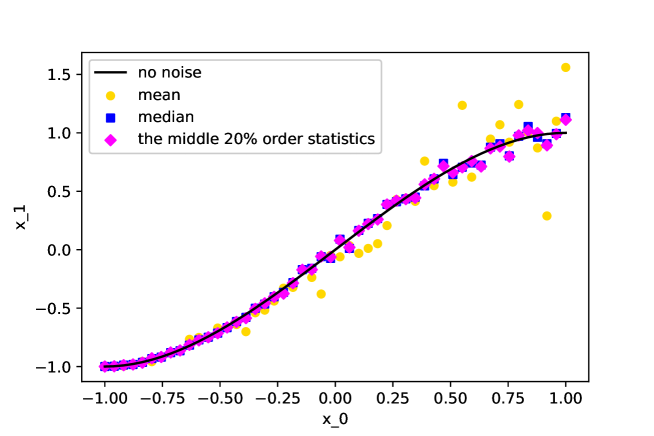
Figure 9: Compare mean (gold dots), median (blue squares), the middle 20% order statistics (magenta diamonds) for the same $x_{0}$. The results show that the middle 20% order statistics is the closest case to no noise differential equation numerical solution (black line). Here the true drift coefficient and diffusion coefficient are $f(X_{t})=-X_{t}^{3}+X_{t}$ and $g(X_{t})=X_{t}+1$, separately.

Appendix C More experimental results

In this appendix, we show more experimental results, including additive/multiplying noise, different $\alpha$ values, different classes of drift coefficients, a two-dimensional SDE with linear drift coefficients and linear diffusion coefficients.

C.1 SDEs driven by Cauchy motion

We maintain the same setting as in Section 4.1.

Additive noise

In addition to what is mentioned in the article, we also consider drift coefficients: $f(X_{t})=-X_{t}+1$ and $f(X_{t})=\sin(X_{t})$. Here we take sample size $N=10000$, $h=0.01$, $x_{0}\in[-3,3]$. The comparison results can be seen in Figure 10. The results of the constant noise intensity are also obtained: $\hat{g}_{\theta}=0.9799$, $\hat{g}_{\theta}=0.9593$.

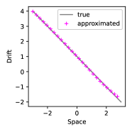
(a) $f(X_{t})=-X_{t}+1$, $\hat{g}_{\theta}=0.9799$

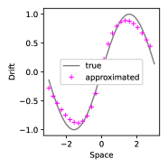
(b) $f(X_{t})=\sin(X_{t})$, $\hat{g}_{\theta}=0.9593$

Figure 10: Cauchy additive noise with different drift coefficients, the gray lines represent the true drift coefficients and the magenta plus markers are the neural networks’ results. $\hat{g}_{\theta}$ represent the diffusion coefficients calculated by (13).

Multiplicative noise

Replacing additive noise with multiplicative noise, we test the multiplier noise as $g(X_{t})=0.1X_{t}+0.5$. Following the construction in the previous section except sample size $N=20$ (different $x_{0}$) $\times 1000$ (sample size), a comparison between the learned and true drift/diffusion functions is shown in Figure 11.

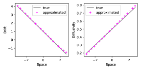
(a) $f(X_{t})=-X_{t}+1$, $g(X_{t})=0.1X_{t}+0.5$, (left) true and approximated drift coefficients, (right) true and approximated diffusivity coefficients

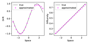
(b) $f(X_{t})=\sin(X_{t})$, $g(X_{t})=0.1X_{t}+0.5$, (left) true and approximated drift coefficients, (right) true and approximated diffusivity coefficients

Figure 11: Cauchy multiplicative noise with different drift coefficients, the gray lines represent the true drift coefficients and true diffusion coefficients, and the magenta plus markers are the estimated drift and diffusion results from our proposed neural networks.

C.2 SDEs driven by $\alpha$-stable Lévy motion

In this section, neural networks are used twice, separately to estimate drift and diffusion. We continue the construction in Section 4.2.

Additive noise

For $\mathbf{\alpha=1.5}$, we test the drift coefficients $f(X_{t})=-X_{t}+1$, $f(X_{t})=-X_{t}^{3}+X_{t}$ and $f(X_{t})=\log(X_{t}+1.5)-|X_{t}+1.5|^{1/3}$ in equation (1), diffusion coefficient $g=1$. The technique mentioned in appendix B is still used. Here we take sample size $N=5\times 1000$, $h=0.1$ for the linear drift coefficient, $N=50\times 1000$, $h=0.5$ for the other two more complex drift coefficients, both cases $x_{0}\in[-1,1]$. The true drift coefficients and the fitting results of the neural network are compared as shown in Figure 12.

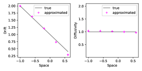
(a) $f(X_{t})=-X_{t}+1$, $g(X_{t})=1$, (left) true and approximated drift coefficients, (right) true and approximated diffusivity coefficients

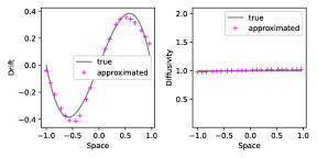
(b) $f(X_{t})=-X_{t}^{3}+X_{t}$, $g(X_{t})=1$, (left) true and approximated drift coefficients, (right) true and approximated diffusivity coefficients

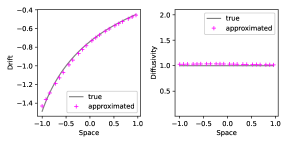
(c) $f(X_{t})=\log(X_{t}+1.5)-|X_{t}+1.5|^{1/3}$, $g(X_{t})=1$, (left) true and approximated drift coefficients, (right) true and approximated diffusivity coefficients

Figure 12: Additive noise with different drift coefficients for $\alpha=1.5$, the gray lines represent the true drift coefficients and true diffusion coefficients, and the magenta plus markers are the estimated drift and diffusion results from our proposed neural networks.

For $\mathbf{\alpha=0.5}$, hyperparameter settings are almost identical. The comparison results are shown in the Figure 13.

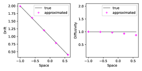
(a) $f(X_{t})=-X_{t}+1$, $g(X_{t})=1$, (left) true and approximated drift coefficients, (right) true and approximated diffusivity coefficients

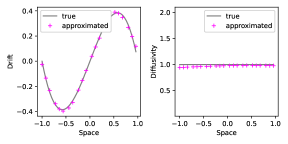
(b) $f(X_{t})=-X_{t}^{3}+X_{t}$, $g(X_{t})=1$, (left) true and approximated drift coefficients, (right) true and approximated diffusivity coefficients

Figure 13: Additive noise with different drift coefficients for $\alpha=0.5$, the gray lines represent the true drift coefficients and true diffusion coefficients, and the magenta plus markers are the estimated drift and diffusion results from our proposed neural networks.

Multiplicative noise

For $\mathbf{\alpha=0.5}$, we test (1) $f(X_{t})=-X_{t}+1$ and $g(X_{t})=X_{t}+1$, $N=5\times 1000$, $h=0.1$; (2) $f(X_{t})=-X_{t}^{3}+X_{t}$ and $g(X_{t})=X_{t}+1$, $N=75\times 1000$, $h=0.5$. The comparison results are shown in the Figure 14.

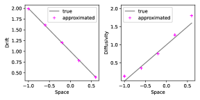
(a) $f(X_{t})=-X_{t}+1$, $g(X_{t})=X_{t}+1$, (left) true and approximated drift coefficients, (right) true and approximated diffusivity coefficients

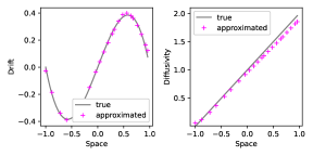
(b) $f(X_{t})=-X_{t}^{3}+X_{t}$, $g(X_{t})=X_{t}+1$, (left) true and approximated drift coefficients, (right) true and approximated diffusivity coefficients

Figure 14: Multiplicative noise with different diffusion coefficients for $\alpha=0.5$, the gray lines represent the true coefficients and the magenta plus markers are the neural networks’ results.

C.3 Another multi-dimensional experiment

In this experiment, the hyperparameter settings are consistent with section 4.2. To demonstrate our capacity to learn multiplicative coupled noise, we examined the approximation of the following SDE:

$$dX_{t} =(X_{t}+Y_{t})dt+(0.5Y_{t}+1)dL_{t,1}^{\alpha},$$ (C1)

$$dY_{t} =(4X_{t}-2Y_{t})dt+(0.5X_{t}+1)dL_{t,2}^{\alpha},$$

where $L_{t,1}^{\alpha}$ and $L_{t,2}^{\alpha}$ are two independent one-dimensional $\alpha$-stable Lévy motions. Here we take $\alpha=1.5$, $N=(5\ \text{different values of}\ x_{0},\ y_{0}\ \text{respectively})\times 1000$, $h=0.5$, $(x_{0},y_{0})\in[-1,1]\times[-1,1]$. The true drift and diffusion coefficients, as well as the approximate results, are also presented as heat maps (Figure 15). As can be seen, our method is still workable.

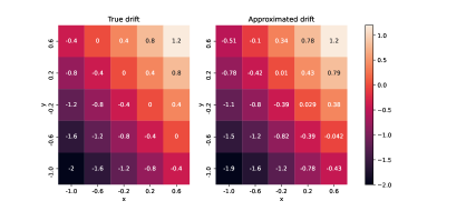
(a) $f_{1}(X_{t},Y_{t})=X_{t}+Y_{t}$, (left) true drift coefficient, (right) approximated drift coefficient

(b) $f_{2}(X_{t},Y_{t})=4X_{t}-2Y_{t}$, (left) true drift coefficient, (right) approximated drift coefficient

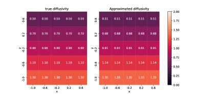
(c) $g_{1}(X_{t},Y_{t})=0.5Y_{t}+1$, (left) true diffusivity coefficient, (right) approximated diffusivity coefficient

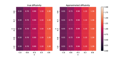
(d) $g_{2}(X_{t},Y_{t})=0.5X_{t}+1$, (left) true diffusivity coefficient, (right) approximated diffusivity coefficient

Figure 15: The drift coefficients (true and estimated) and diffusion coefficients (true and estimated) of the model (C1), presented as heat maps.

References

- [BAA17] Mohammadreza Hassannejad Bibalan, Hamidreza Amindavar, and Maryam Amirmazlaghani, “Characteristic function based parameter estimation of skewed alpha-stable distribution: An analytical approach,” Signal Processing 130, 323–336 (2017).
- [BHW05] Szymon Borak, Wolfgang Härdle, and Rafał Weron, Statistical tools for finance and insurance, 21–44 (Springer, 2005).
- [BMA10] Harish Bhaskar, Lyudmila S. Mihaylova, and Alin Achim, “Video foreground detection based on symmetric alpha-stable mixture models,” IEEE Transactions on Circuits and Systems for Video Technology 20, 1133–1138 (2010).
- [BPK16] Steven L. Brunton, Joshua L. Proctor, and J. Nathan Kutz, “Discovering governing equations from data by sparse identification of nonlinear dynamical systems,” Proceedings of the National Academy of Sciences 113, 3932 – 3937 (2016).
- [CCD+17] Rui Cai, Xiaoli Chen, Jinqiao Duan, Jürgen Kurths, and Xiaofang Li, “Lévy noise-induced escape in an excitable system,” Journal of Statistical Mechanics: Theory and Experiment, 2017, 063503 (2017).
- [CRBD18] Ricky T. Q. Chen, Yulia Rubanova, Jesse Bettencourt, and David Kristjanson Duvenaud, “Neural ordinary differential equations,” Advances in Neural Information Processing Systems 31 (2018).
- [CYDK21] Xiaoli Chen, Liu Yang, Jinqiao Duan, and George Em Karniadakis, “Solving inverse stochastic problems from discrete particle observations using the fokker-planck equation and physics-informed neural networks,” SIAM Journal on Scientific Computing 43, B811–B830 (2021).
- [DDF21] Noura Dridi, Lucas Drumetz, and Ronan Fablet, “Learning stochastic dynamical systems with neural networks mimicking the euler-maruyama scheme,” 2021 29th European Signal Processing Conference (EUSIPCO), 1990–1994 (2021).
- [DGL+20] Min Dai, Ting Gao, Yubin Lu, Yayun Zheng, and Jinqiao Duan, “Detecting the maximum likelihood transition path from data of stochastic dynamical systems,” Chaos 30, 113124 (2020).
- [DMK+21] Felix Dietrich, Alexei Makeev, George Kevrekidis, Nikolaos Evangelou, Tom S. Bertalan, Sebastian Reich, and Ioannis G. Kevrekidis, “Learning effective stochastic differential equations from microscopic simulations: combining stochastic numerics and deep learning,” ArXiv abs/2106.09004 (2021).
- [Dua15] Jinqiao Duan, An introduction to stochastic dynamics, volume 51 (Cambridge University Press, 2015).
- [Fer78] Thomas S. Ferguson, “Maximum likelihood estimates of the parameters of the cauchy distribution for samples of size 3 and 4,” Journal of the American Statistical Association 73, 211–213 (1978).
- [GOF+17] Constantino A. García, Abraham Otero, Paulo Félix, Jesús María Rodríguez Presedo, and David G. Márquez, “Nonparametric estimation of stochastic differential equations with sparse gaussian processes,” Physical Review. E 96, 2, 022104 (2017).
- [GPAM+14] Ian J. Goodfellow, Jean Pouget-Abadie, Mehdi Mirza, Bing Xu, David Warde-Farley, Sherjil Ozair, Aaron C. Courville, and Yoshua Bengio, “Generative adversarial nets,” Advances in neural information processing systems 27 (2014).
- [HSSL11] Yanling Hao, Zhiming Shan, Feng Shen, and Dongze Lv, “Parameter estimation of alpha-stable distributions based on mcmc,” 2011 3rd International Conference on Advanced Computer Control, IEEE, 325–327 (2011).
- [HZRS16] Kaiming He, X. Zhang, Shaoqing Ren, and Jian Sun, “Deep residual learning for image recognition,” Proceedings of the IEEE Conference on Computer Vision and Pattern Recognition (CVPR), 770–778 (2016).
- [IH98] Jacek Ilow and Dimitrios Hatzinakos, “Applications of the empirical characteristic function to estimation and detection problems,” Signal Processing 65, 199–219 (1998).
- [JB19] Junteng Jia and Austin R. Benson, “Neural jump stochastic differential equations,” Advances in Neural Information Processing Systems 32 (2019).
- [JMW12] Benjamin Jourdain, Sylvie Méléard, and Wojbor A. Woyczynski, “Lévy flights in evolutionary ecology,” Journal of Mathematical Biology 65, 677–707 (2012).
- [KNP+19] Stefan Klus, Feliks Nuske, Sebastian Peitz, Jan-Hendrik Niemann, Cecilia Clementi, and Christof Schutte, “Data-driven approximation of the koopman generator: Model reduction, system identification, and control,” Physica D: Nonlinear Phenomena 406, 132416 (2020).
- [KW14] Diederik P. Kingma and Max Welling, “Auto-encoding variational bayes,” ArXiv abs/1312.6114 (2014).
- [LD20a] Yang Li and Jinqiao Duan, “A data-driven approach for discovering stochastic dynamical systems with non-gaussian lévy noise,” Physica D: Nonlinear Phenomena 417, 132830 (2021).
- [LD20b] Yubin Lu and Jinqiao Duan, “Discovering transition phenomena from data of stochastic dynamical systems with lévy noise,” Chaos 30, 093110 (2020).
- [LD21] Yang Li and Jinqiao Duan, “Extracting governing laws from sample path data of non-gaussian stochastic dynamical systems,” Journal of Statistical Physics 186, 30 (2022).
- [LDLZ20] Yang Li, Jinqiao Duan, Xianbin Liu, and Yanxia Zhang, “Most probable dynamics of stochastic dynamical systems with exponentially light jump fluctuations,” Chaos 30, 063142 (2020).
- [LLD21] Yubin Lu, Yang Li, and Jinqiao Duan, “Extracting stochastic governing laws by nonlocal kramers-moyal formulas,” ArXiv abs/2108.12570 (2021).
- [LLXD21] Yang Li, Yubin Lu, Shengyuan Xu, and Jinqiao Duan, “Extracting stochastic dynamical systems with alpha-stable Lévy noise from data,” Journal of Statistical Mechanics: Theory and Experiment 2022.2, 023405 (2022).
- [LWCD20] Xuechen Li, Ting-Kam Leonard Wong, Ricky T. Q. Chen, and David Kristjanson Duvenaud, “Scalable gradients for stochastic differential equations,” International Conference on Artificial Intelligence and Statistics PMLR, 3870–3882 (2020).
- [McC86] J. Huston McCulloch, “Simple consistent estimators of stable distribution parameters,” Communications in Statistics-Simulation and Computation 15(4), 1109–1136 (1986).
- [MDC+99] Stefan Mittnik, S.T. Rachev, T. Doganoglu, D. Chenyao, “Maximum likelihood estimation of stable paretian models,” Mathematical and Computer modelling 29(10-12), 275–293 (1999).
- [NA11] Jean-Marie Nicolas and Stian Normann Anfinsen, “Introduction to second kind statistics: Application of log-moments and log-cumulants to the analysis of radar image distributions,” Trait. Signal 19(3), 139–167 (2011).
- [NBD+21] Alexander Norcliffe, Cristian Bodnar, Ben Day, Jacob Moss, and Pietro Liò, “Neural ode processes,” ArXiv, abs/2103.12413 (2021).
- [Nol01] John P. Nolan, “Maximum likelihood estimation and diagnostics for stable distributions,” Lévy Processes: Theory and Applications, 379–400 (Birkhäuser Boston, 2001).
- [Nol03] John P. Nolan, “Modeling financial data with stable distributions,” Handbook of Heavy Tailed Distributions in Finance, 105–130 (North-Holland, 2003).
- [Nol13] John P. Nolan, “Multivariate elliptically contoured stable distributions: theory and estimation,” Computational Statistics 28, 2067–2089 (2013).
- [Opp19] Manfred Opper, “Variational inference for stochastic differential equations,” Annalen der Physik 531(3), 1800233 (2019).
- [RBO13] Andreas Ruttor, Philipp Batz, and Manfred Opper, “Approximate gaussian process inference for the drift function in stochastic differential equations,” Advances in Neural Information Processing Systems 26 (2013).
- [RGMP18] Tom Ryder, Andrew Golightly, Andrew Stephen McGough, and Dennis Prangle, “Black-box variational inference for stochastic differential equations,” International Conference on Machine Learning PMLR, 4423–4432 (2018).
- [ST95] Gennady Samorodnitsky and Murad S. Taqqu, Stable non-gaussian random processes: Stochastic models with infinite variance: Stochastic Modeling (Routledge, 1994).
- [TR19] Belinda Tzen and Maxim Raginsky, “Neural stochastic differential equations: Deep latent gaussian models in the diffusion limit,” ArXiv, abs/1905.09883 (2019).
- [Wan21] Bingzhang Wang, “Parameter Estimation of Cauchy Distribution,” Mathematics in Practice and Theory 51(1), 258–264 (2021).
- [Woy01] Wojbor A. Woyczyński, “Lévy processes in the physical sciences,” Lévy processes, 241–266 (Birkhäuser, 2001).
- [XD21] Kailai Xu and Eric F Darve, “Solving inverse problems in stochastic models using deep neural networks and adversarial training,” Computer Methods in Applied Mechanics and Engineering 384, 113976 (2021).
- [YZD+20] Fang Yang, Yayun Zheng, Jinqiao Duan, Ling Fu, and Stephen Wiggins, “The tipping times in an arctic sea ice system under influence of extreme events,” Chaos 30, 063125 (2020).
- [Zha91] Wenzhong Zhang, Ruyu Dan, Counterexamples in probability statistics (in Chinese). (University of Electronic Science and Technology of China Press, 1991).