Abstract.

In personalized Federated Learning, each member of a potentially large set of agents aims to train a model minimizing its loss function averaged over its local data distribution. We study this problem under the lens of stochastic optimization. Specifically, we introduce information-theoretic lower bounds on the number of samples required from all agents to approximately minimize the generalization error of a fixed agent. We then provide strategies matching these lower bounds, in the all-for-one and all-for-all settings where respectively one or all agents desire to minimize their own local function. Our strategies are based on a gradient filtering approach: provided prior knowledge on some notions of distances or discrepancies between local data distributions or functions, a given agent filters and aggregates stochastic gradients received from other agents, in order to achieve an optimal bias-variance trade-off.

1. Introduction

A central task in Federated Learning (McMahan et al., 2017; Kairouz et al., 2019) is the training of a common model from local data sets held by individual agents. A typical application is when users (e.g. mobile phones, hospitals) want to make predictions (e.g. next-word prediction, treatment prescriptions), but each has access to very few data samples, hence the need for collaboration. As highlighted by many recent works (e.g. Hanzely et al. (2020); Mansour et al. (2020)), while training a global model yields better statistical efficiency on the combined datasets of all agents by increasing the number of samples linearly in the number of agents, this approach can suffer from a dramatically poor generalization error on local datasets. A solution to this generalization issue is the training of personalized models, a midway between a shared model between agents and models trained locally without any coordination.

An ideal approach would take the best of both worlds: increased statistical efficiency by using more samples, while keeping local generalization errors low. This raises the fundamental question: what is the optimal bias/variance tradeoff between personalization and coordination, and how can it be achieved?

We formulate the personalized federated learning problem as follows, studying it under the lens of stochastic optimization (Bottou et al., 2018). Consider $N\in\mathbb{N}^{*}$ agents denoted by integers $1\leqslant i\leqslant N$, each desiring to minimize its own local function $f_{i}:\mathbb{R}^{d}\to\mathbb{R}$, while sharing their stochastic gradients. Since only a limited number of samples are locally available, we focus on stochastic gradient descent-like algorithms, where agents each sequentially compute stochastic gradients $g_{i}^{k}$ such that $\mathbb{E}\left[g_{i}^{k}\right]=\nabla f_{i}$. In order to reduce the sample complexity, i.e. the number of samples or stochastic gradients required to reach small generalization error, agents thus need to use stochastic gradients from other agents, that are biased since in general $\mathbb{E}\left[g_{i}^{k}\right]\neq\nabla f_{j}$. We first consider the all-for-one objective, where a single agent $i$ wants to minimize its local function (local generalization error), using its own information as well as information from agents $j\neq i$. We then address the all-for-all objective where all agents want to minimize their local function (local generalization error) in parallel using shared information. Our algorithms are based on a gradient filtering approach: in both all-for-one and all-for-all objectives, upon reception of stochastic gradients $(g_{j}^{k})_{j}$, agent $i$ filters these gradients and aggregates them using some weights $\lambda_{j}$ into $\sum_{j}\lambda_{j}g_{j}^{k}$, in order to achieve some bias/variance trade-off.

Contributions and outline of the paper

In this paper, we consider oracle models where at each step $k=1,2,\dots$, one (or all) agent(s) may draw a sample according to its (their) local distribution. We aim at computing the number of stochastic gradients sampled from all agents, required to reach a small generalization error in both all-for-one and all-for-all formulations, in terms of: biases (distances between functions or distributions), regularity and noise assumptions. The oracle models, main assumptions and problem formulations are given in Section 2. Our main contributions are then as follows:

(i) In Section 3 we prove information theoretic lower bounds: to reach a target generalization error $\varepsilon>0$ for a fixed agent $i$, no algorithm can achieve a reduction in the number of oracle calls by a factor larger than the total number of agents $\varepsilon$-close –in a suitable sense– to agent $i$.

(ii) We next study a weighted gradient averaging algorithm for the all-for-one problem, matching this lower bound.

(iii) We then propose in Section 5 a parallel extension of the simple weighted gradient averaging algorithm that yields an efficient algorithm for the all-for-all problem. In this algorithm, agents compute stochastic gradients at their local estimate, and broadcast it to other agents who may use these to update their own estimates. For $x^{k}=(x_{1}^{k},\ldots,x_{N}^{k})$ where $x_{i}^{k}$ is the local estimate of agent $i$ at iteration $k$, updates of the all-for-all algorithm write as:

$$x^{k+1}=x^{k}-\eta Wg^{k}\,,$$

where $g^{k}=(g_{1}^{k},...,g_{N}^{k})$ for an unbiased stochastic gradient $g_{i}^{k}$ of function $f_{i}$, a step size $\eta$, and a carefully chosen matrix $W$. Agents $i$ thus use stochastic gradients that are doubly biased, as gradients of a “wrong function” $f_{j}$ instead of $f_{i}$ computed at a “wrong location” $x^{k}_{j}$ instead of $x^{k}_{i}$.

Related works

Federated Learning is a paradigm in machine learning where training is done collaboratively among several agents, taking into account privacy constraints (McMahan et al., 2017; Konečný et al., 2016; Kairouz et al., 2019; Wang et al., 2019). A central task is the training of a common model for all agents, for which both centralized approaches orchestrated by a server and decentralized approaches with no central coordinator (Nedich et al., 2018) have been considered. The algorithms we propose in this paper are well suited for a decentralized implementation.

As observed in Hanzely et al. (2020), training a common model for all users can lead to poor generalization on certain tasks such as e.g. next-word prediction. To improve both accuracy and fairness, personalized models thus need to be learnt for each agent (Li et al., 2020; Mohri et al., 2019; Yu et al., 2021). Approaches to personalization include fine-tuning (Cheng et al., 2021; Khodak et al., 2019), transfer learning techniques (Tripuraneni et al., 2020; Wang et al., 2019). Hanzely et al. (2020); Fallah et al. (2020) among others formulate personalization in FL as the training of local models with a regularization term that enforces collaboration between users. We refer the interested reader to Kulkarni et al. (2020) for a broader survey of Personalized Federated Learning.

While the goal of personalization is to minimize local generalization errors, the above cited works do not provide theoretical guarantees over the sample complexity to obtain small local errors, but instead control errors on a regularized problem, in terms of communication rounds or full gradients used, and not in terms of samples used. Deng et al. (2020); Mansour et al. (2020) among others provide generalization errors under a statistical learning framework that depend on VC-dimensions and on distances between each local data distribution and the mixture of all datasets. Donahue and Kleinberg (2021a, b) study the bias-variance trade-off between collaboration and personalization for mean estimation in a game-theoretic framework. Chayti et al. (2021); Grimberg et al. (2021); Beaussart et al. (2021) frame personalization as a stochastic optimization problem with biased gradients and are the works closest to ours. They consider the training of a single agent with biased gradients from another group of agents, i.e. the all-for-one problem and obtain performance guarantees in terms of distance between individual function $f_{i}$ and the average $N^{-1}\sum_{j}f_{j}$. In contrast, we obtain more general performance bounds based on distance bounds between all pairs of functions $f_{i}$, $f_{j}$ (or equivalently, pairs of local distributions). In addition, we prove matching lower bounds. Finally, we also consider the all-for-all problem, for which we obtain efficient algorithms, and leverage in that setting the use of weaker bias assumptions than in the all-for-one problem.

2. Problem Statement and Assumptions

We now detail our objectives and the necessary technical assumptions. We consider general stochastic gradient methods and formulate our problems, assumptions and algorithms accordingly. Our lower bounds apply to a more specific problem, namely generalization error minimization, or GEM, where functions $f_{j}$ of all agents $j$ are all obtained from the same loss function $\ell$. These lower bounds a fortiori apply to the more general stochastic gradient setup of our algorithms.

Stochastic (sub)-gradients

Let $f_{i}:\mathbb{R}^{d}\to\mathbb{R}$, $1\leqslant i\leqslant N$ be agent $i$’s local function to be minimized (e.g. the average of a loss function over its local data distribution). At every iteration $k=1,2,\ldots$, agent $i$ may access unbiased i.i.d. estimates $g_{i}^{k}(x)$ of $\nabla f_{i}(x)$ (or of some subgradient $s(x)\in\partial f_{i}(x)$, depending on the regularity assumptions made):

$$\mathbb{E}\left[g_{i}^{k}(x)\right]\in\partial f_{i}(x)\,,\quad x\in\mathbb{R}^{d}\,,\,k\geqslant 0\,,\,1\leqslant i\leqslant N\,.$$

We consider two different objectives. In the all-for-one setting, using information from all agents, a fixed agent $i$ desires to minimize its own local function $f_{i}$ (typically, in collaborative GEM, $f_{i}$ is the generalization error $f_{i}(x)=\mathbb{E}_{\mathcal{D}_{i}}[\ell(x,\xi_{i})]$). In the all-for-all setting, all agents want to minimize their own local function, using shared information.

Oracle models

To specify the information shared between agents via access to stochastic gradients, we define the following oracles. The synchronous oracle (resp. asynchronous oracle) lets at every iteration all agents (resp. only one agent) sample a stochastic gradient. After $K$ queries from the synchronous oracle (resp. asynchronous oracle), each agent will have sampled $K$ (resp. $K/N$ on average) stochastic gradients for a total of $NK$ (resp. $K$) in the whole set of agents. In the all-for-one setting where a fixed agent $i$ desires to minimize its own local function $f_{i}$, all agents $j$ can take the same $x_{j}^{k}=x_{i}^{k}$ as argument of their stochastic gradient, resulting in a simple stochastic gradient descent with biased gradients. The difficulty in analyzing all-for-all algorithms lies in the fact that stochastic gradients sampled by agent $j$ are doubly biased for agent $i$, being potentially computed at some $x_{j}^{k}$ distinct from $x_{i}^{k}$.

Synchronous and asynchronous oracles At iterations $k=1,2,...$: 1: A set of agents $S^{k}$ is chosen: $S^{k}={{\left\{1,\ldots,N\right\}}}$ for the synchronous oracle, $S^{k}={{\left\{i_{k}\right\}}}$ where $i_{k}$ is sampled uniformly at random amongst agents, for the asynchronous oracle. ; 2: For all $j\in S^{k}$, agent $j$ chooses some $y_{j}^{k}$ as a (possibly random) function of all previous stochastic gradients and iterates, and samples $g_{j}^{k}(y_{j}^{k})$; 3: All agents can then perform an update using these new stochastic gradients and all previous ones.

For fixed target precision $\varepsilon>0$, the objective is to find, using $T_{\varepsilon}$ samples from all agents in total, queried with synchronous or asynchronous oracles, models with local generalization error $\varepsilon$. We prove matching lower and upper bounds on the sample complexity $T_{\varepsilon}$ in the all-for-one and all-for-all settings.

Regularity, Bias and Noise Assumptions

Throughout the paper, we assume that each function $f_{i}$ is minimized over $\mathbb{R}^{d}$, and we denote by $x_{i}^{\star}$ such a minimizer.

Bias assumptions on function discrepancies. For some non-negative weights $(b_{ij})_{1\leqslant i,j\leqslant N}\in{\mathbb{R}^{+}}^{N\times N}$, $(\tilde{b}_{ij})_{1\leqslant i,j\leqslant N}\in{\mathbb{R}^{+}}^{N\times N}$ and $m\geqslant 0$, either one of the two following assumptions will be made. Note that if differentiable, we have $\mathbb{E}\left[g_{i}^{k}(x)\right]=\nabla f_{i}(x)$.

1. For all $1\leqslant i,j\leqslant N$, optimal model $x_{j}^{\star}$ for $j$ generalizes (with generalization error $b_{ij}$) for agent $i$:

   $$f_{i}(x_{j}^{\star})-f_{i}(x_{i}^{\star})\leqslant b_{ij}\,.$$ (1)

2. For all $1\leqslant i,j\leqslant N$ and for all $x\in\mathbb{R}^{d}$, $k\geqslant 0$:

   $${{\left\|\mathbb{E}\left[g_{i}^{k}(x)\right]-\mathbb{E}\left[g_{j}^{k}(x)\right]\right\|}}^{2}\leqslant\tilde{b}_{ij}\,.$$ (2)

Two sets of regularity and noise assumptions. The two different noise and regularity assumptions we shall consider are as follows.

1. For all $1\leqslant i\leqslant N$, $f_{i}$ is convex and for some $B>0$, all $k\geqslant 1$ and $x\in\mathbb{R}^{d}$,

   $$\mathbb{E}\left[{{\left\|g_{i}^{k}(x)\right\|}}^{2}\right]\leqslant B^{2}\,.$$ (3)

2. For all $1\leqslant i\leqslant N$, $f_{i}$ $\mu$-strongly convex, $L$-smooth, and we write $\kappa=\frac{L}{\mu}$. For $\sigma>0$, all $k\geqslant 1$ and $x\in\mathbb{R}^{d}$:

   $$\mathbb{E}\left[{{\left\|g_{i}^{k}(x)-\nabla f_{i}(x)\right\|}}^{2}\right]\leqslant\sigma^{2}\,.$$ (4)

Our regularity assumptions are standard; our bias (and gradient dissimilarity) assumptions are less classical, and can be derived from Wassertstein-like distribution-based distances in the GEM setting (Section 6 and Appendix A). Assumption (B.2) will be used in the all-for-one setting, while the less restrictive (B.1) will be used in the all-for-all setting. It quantifies by how much agents’ objectives differ. To the best of our knowledge it has not been previously used in Federated Learning. It is related to (B.2) through $f_{i}(x_{j}^{\star})-f_{i}(x_{i}^{\star})\leqslant\frac{1}{2\mu}{{\left\|\nabla f_{i}(x_{j}^{\star})-\nabla f_{i}(x_{i}^{\star})\right\|}}^{2}=\frac{1}{2\mu}{{\left\|\nabla f_{i}(x_{j}^{\star})\right\|}}^{2}$ under $\mu$-PL or strong convexity assumptions. More generally, we always have $f_{i}(x_{j}^{\star})-f_{i}(x_{i}^{\star})\leqslant{{\left\|x_{i}^{\star}-x_{j}^{\star}\right\|}}{{\left\|\nabla f_{i}(x_{j}^{\star})\right\|}}$. Our lower bounds apply to functions that verify both these bias assumptions, and a fortiori verify the assumptions made in our upper bounds where only one of these bias assumptions is required.

Finally, our upper bounds will use the following settings, that we refer to as Setting 1 and Setting 2:

1. Asynchronous oracle is used, assumption (N.1) holds.

2. Synchronous oracle is used, assumption (N.2) holds.

A key instance of our problem is collaborative generalization error minimization (GEM): let $\mathcal{D}_{i}$ for $1\leqslant i\leqslant N$ be a probability distribution on a set $\Xi$ (agent $i$’s local distribution, not its empirical distribution), $\ell:\mathcal{X}\times\Xi\to\mathbb{R}$ a loss function, and define the following local objective function, that agent $i$ aims at minimizing:

$$f_{i}(x)=\mathbb{E}_{\xi_{i}\sim\mathcal{D}_{i}}\left[\ell(x,\xi_{i})\right]\,,\quad x\in\mathcal{X}\,.$$ (5)

Function $f_{i}$ is thus the generalization error on agent $i$’s local distribution. Stochastic gradients are in that case of the form $g_{i}^{k}(x)=\nabla_{x}\ell(x,\xi_{i}^{k})$ where $\xi_{i}^{k}\sim\mathcal{D}_{i}$. Counting the number of stochastic gradients used in the whole set of agents to reach a precision $\varepsilon$ for $f_{i}$ thus reduces to computing the number of samples required from all agents to obtain local generalization error $\varepsilon$ for agent $i$. In Appendix A we discuss how our bias assumptions follow from bounds on distances between distributions $\mathcal{D}_{i}$, $\mathcal{D}_{j}$ together with practical scenarios where such bounds can be obtained.

Notation: in the rest of the paper, variables $t$ or $T$ denote the number of stochastic gradients $g_{i}^{k}$ sampled (or data item sampled from personal distribution) from all agents, while variables $k$ or $K$ denote the iterates of the algorithms or equivalently to the number of oracle calls made.

3. IT Lower Bounds on the Sample Complexity

In this section, we prove lower bounds on the sample complexity of the all-for-one problem. Our lower bounds apply to collaborative GEM, i.e. functions $(f_{i})_{1\leqslant i\leqslant N}$ of the form (5), for some shared loss function $\ell$ and user distributions $\mathcal{D}_{1},\ldots,\mathcal{D}_{N}$.

An oracle $\phi:\mathbb{R}^{N\times d}\to\mathcal{I}$ is a random function that answers some $\phi(x)\in\mathcal{I}$ where $\mathcal{I}$ is an information set, for every query $x\in\mathbb{R}^{N\times d}$. We adapt the definitions of Agarwal et al. (2012) of sample complexity for SGD to our personalization problem. Formally, the first-order oracle we defined in Section 2 (for either synchronous or asynchronous oracles) and that we write as $\phi\big{(}(\mathcal{D}_{i})_{i=1,\ldots,N},\ell\big{)}$ for shared loss function $\ell$ and user distributions $\mathcal{D}_{1},\ldots,\mathcal{D}_{N}$, returns for $x\in\mathbb{R}^{N\times d}$:

$$\phi\big{(}(\mathcal{D}_{i})_{i},\ell\big{)}(x)=\Big{(}i,\,x_{i},\,\xi_{i},\,\ell(x_{i},\xi_{i}),\,g_{i}^{k}(x_{i})\Big{)}_{i\in S^{k}}\,,$$

where $\xi_{i}\sim\mathcal{D}_{i}$ and $S^{k}$ is the set of agents returning a stochastic gradient at step $k$, according to the synchronous or asynchronous oracle in use. Given distributions and a loss function $\big{(}(\mathcal{D}_{i})_{i},\ell\big{)}$, we denote by $\mathbb{M}$ the set of all methods $\mathcal{M}=(\mathcal{M}_{T})_{T\geqslant 0}$: for any $T\geqslant 0$, $\mathcal{M}_{T}$ makes $K$ oracle calls from oracle $\phi\big{(}(\mathcal{D}_{i})_{i},\ell\big{)}$ while using $T$ stochastic gradient samples from all agents ($T=NK$ with the synchronous oracle, $T=K$ with the asynchronous oracle), and returns $x_{i}^{T}\in\mathbb{R}^{d}$ for agent $i$. For a set $\mathbb{D}$ of couples of distributions and loss function $\big{(}(\mathcal{D}_{j})_{j},\ell\big{)}$ defining functions $(f_{i})_{1\leqslant i\leqslant N}$, we are interested in lower-bounding:

$$\inf_{\mathcal{M}\in\mathbb{M}}\sup_{((\mathcal{D}_{j})_{j},\ell)\in\mathbb{D}}\mathcal{T}_{i}^{\varepsilon}\Big{(}\mathcal{M},\big{(}(\mathcal{D}_{j})_{j},\ell\big{)}\Big{)}\,,$$

where $\mathcal{T}_{i}^{\varepsilon}\Big{(}\mathcal{M},\big{(}(\mathcal{D}_{j})_{j},\ell\big{)}\Big{)}$ is the number of samples required from all agents (uniformly divided between agents) to reach generalization error $\varepsilon>0$ for agent $i$ and writes as:

$$\inf{{\left\{T\in\mathbb{N}^{*}\,\text{such that}\,\mathbb{E}\left[f_{i}(x_{i}^{T})-\min_{x\in\mathcal{X}}f_{i}(x)\right]\leqslant\varepsilon\right\}}}\,.$$

For $(b_{ij})\in{\mathbb{R}^{+}}^{N\times N}$, $r>0$, $B>0$, let $\mathbb{D}(r,b,B)$ be the set of all $\big{(}(\mathcal{D}_{i})_{1\leqslant i\leqslant N},\ell\big{)}$ for probability distributions $(\mathcal{D}_{i})_{1\leqslant i\leqslant N}$ on a probability space $\Xi\subset\mathbb{R}^{D}$ such that all functions $f_{i}$ parameterized by the losses and distributions in this set verify ${{\left\|x_{i}^{\star}\right\|}}\leqslant r$, assumption (N.1), and bias assumptions (B.1) and (B.2) for $b$ and $\tilde{b}_{ij}=(b_{ij}/r)^{2}$.

Similarly, for $\sigma>0$, $\mu,L>0$, let $\mathbb{D}_{\mu}^{L}(r,b,B)$ be the set of all $\big{(}(\mathcal{D}_{i})_{1\leqslant i\leqslant N},\ell\big{)}$ for probability distributions $(\mathcal{D}_{i})_{1\leqslant i\leqslant N}$ on a probability space $\Xi\subset\mathbb{R}^{D}$ such that all functions $f_{i}$ parameterized by this set verify ${{\left\|x_{i}^{\star}\right\|}}\leqslant r$, assumption (N.2), and bias assumptions (B.1) and (B.2) for $b$ and $\tilde{b}=\mu b$ here.

Theorem 1 (IT lower bound).

Let $\varepsilon\in(0,1/16)$, and assume that either the synchronous or asynchronous oracle is used, that $(b_{ij})$ verifies the triangle inequality $b_{ij}\leqslant b_{ik}+b_{kj}$ for all $1\leqslant i,j,k\leqslant N$. For some constant $C>0$ independent of the problem and any $i\in\{1,\ldots,N\}$:

$$\inf_{\mathcal{M}\in\mathbb{M}}\!\sup_{((\mathcal{D}_{j})_{j},\ell)\in\mathbb{D}(r,b,B)}\!\!\!\!\!\!\mathcal{T}_{i}^{\varepsilon}\Big{(}\mathcal{M},\big{(}(\mathcal{D}_{j})_{j},\ell\big{)}\Big{)}\!\geqslant\!\frac{Cr^{2}B^{2}N}{\varepsilon^{2}\mathcal{N}_{i}^{\varepsilon}(\frac{b}{4})}\,,$$

where $\mathcal{N}_{i}^{\varepsilon}(b)=\sum_{j}\mathds{1}_{\{b_{ij}\leqslant\varepsilon\}}$ is the number of agents $j$ verifying $b_{ij}\leqslant\varepsilon$. Under strong-convexity and smoothness assumptions for $\mu=L=1/r^{2}$, we have, for some $C^{\prime}>0$:

$$\inf_{\mathcal{M}\in\mathbb{M}}\!\sup_{((\mathcal{D}_{j})_{j},\ell)\in\mathbb{D}_{\mu=1/r^{2}}^{L=1/r^{2}}(r,b,\sigma)}\!\!\!\!\!\!\mathcal{T}_{i}^{\varepsilon}\Big{(}\mathcal{M},\big{(}(\mathcal{D}_{j})_{j},\ell\big{)}\Big{)}\geqslant\frac{C^{\prime}r^{2}\sigma^{2}N}{\varepsilon\mathcal{N}_{i}^{\varepsilon}(\frac{b}{4})}\,.$$

The proof of these lower bounds (Appendix B) builds on lower bounds based on Fano’s inequality (Duchi and Wainwright, 2013) for stochastic gradient descent Agarwal et al. (2012) or for information limited statistical estimation (Zhang et al., 2013; Duchi and Rogers, 2019), adapted to personalization.

Lower-bound interpretation. Theorem 1 states that, given the knowledge of $(b_{ij})$ and $B^{2}$ (or $\sigma^{2}$, $\mu$ and $L$), there exist difficult instances of the problem that satisfy assumption (N.1) (or (N.2)) and both bias assumptions (B.1) and (B.2) for $b$, such that the number of samples from all agents (generated through the synchronous or asynchronous oracle) needed to obtain a generalization error of $\varepsilon$ for an agent $i$ is lower-bounded by the right hand sides of the equations in Theorem 1.

Collaboration speedup. The factor $N\times CB^{2}r^{2}\varepsilon^{-2}$ is reminiscent of stochastic gradient descent, and is present in Agarwal et al. (2012): without cooperation, this is the sample complexity of SGD for a fixed agent (for $T$ samples from all agents, only $T/N$ are taken from a given agent $i$). Cooperation appears in the factor $1/\mathcal{N}_{i}^{\varepsilon}(b/4)$: the sample complexity is inversely proportional to the number of agents $j$ that have functions (or distributions) similar to that of $i$. One cannot hope for better than a linear speedup proportional to agents $\varepsilon/4$-close to $i$, in the sense that the functions parameterized by the loss function and distributions verify $f_{i}(x_{j}^{\star})-f_{i}(x_{i}^{\star})\leqslant b_{ij}/4$ and ${{\left\|\nabla f_{i}(x)-\nabla f_{j}(x)\right\|}}^{2}\leqslant\tilde{b}_{ij}$ for all $x\in\mathbb{R}^{d}$, where $\tilde{b}=(b/r)^{2}$ in the first case, and $\tilde{b}=b/r^{2}=\mu b$ in the second.

Bias assumptions and collaborative GEM. In Section 6, we relate ${{\left\|\nabla f_{i}-\nabla f_{j}\right\|}}$ to distribution-based distances $d_{\mathcal{H}}(\mathcal{D}_{i},\mathcal{D}_{j})$ in the GEM setting, where $d_{\mathcal{H}}$ is a 1-Wassertstein-like distance. We prove that the distributions leading to the functions used to prove Theorem 1 verify $d_{\mathcal{H}}(\mathcal{D}_{i},\mathcal{D}_{j})\leqslant b_{ij}$; thus, the distribution based distances also sharply characterize the sample complexity. The requirement for the lower bound to apply that $(b_{ij})$ verifies the triangle inequality is thus quite natural, when translating bias assumptions into distribution-based distances.

4. Weighted Gradient Averaging is optimal in the All-for-one setting

We now prove that a weighted gradient averaging (WGA) algorithm is optimal in the all-for-one setting. Fix the agent $i$ who desires to minimize its local function $f_{i}$ (no longer assumed to derive from a loss function). The iterates of the weighted gradient averaging algorithm write as, for both synchronous and asynchronous oracles:

$$x^{k+1}=x^{k}-\eta\sum_{j=1}^{N}\lambda_{j}G^{k}(x)_{j}\,,$$ (6)

for some step size $\eta>0$ and stochastic vector $\lambda\in\mathbb{R}^{N}$, and:

$$G^{k}(x)_{i}=\left\{\begin{aligned} &N\mathds{1}_{{{\left\{i=i_{k}\right\}}}}g_{i_{k}}^{k}(x)\quad\text{(asynchronous)}\\ &g_{i}^{k}(x)\,\,\,\,\,\quad\quad\quad\text{(synchronous oracle)}\,.\end{aligned}\right.$$ (7)

In the WGA algorithm, all agents involved keep the same local estimates $x_{i}^{k}$. As defined in Section 2, $(g_{i}^{k})$ are i.i.d. non-biased stochastic (sub)gradients of functions $f_{i}$. The WGA algorithm thus defined is more general than previous ones, through the introduction of parameter $\lambda$. In the GEM setting, WGA is equivalent to training a model on the mixture of distributions $(\mathcal{D}_{j})_{j}$, with weights $(\lambda_{j})_{j}$. We have the following convergence guarantees in terms of sample complexity for the minimization of a function $f_{i}$ with WGA iterations.

Theorem 2.

Let $\varepsilon>0$, and set $\lambda_{j}=\frac{\mathds{1}_{{{\left\{b_{ij}<\varepsilon/2\right\}}}}}{\mathcal{N}_{i}^{\varepsilon}(2b)}$, $\mathcal{N}_{i}^{\varepsilon}$ being defined in Theorem 1. Generate $(x^{k})_{k}$ using (6).

1. Under Setting 1. Assume that for all $k\geqslant 0$ and $i$, ${{\left\|x^{k}-x_{i}^{\star}\right\|}}\leqslant D$ for some $D>0$ and bias assumption (B.2) holds for $\tilde{b}=(b/D)^{2}$. For $K=T_{\varepsilon}$ and for $\eta=\sqrt{\frac{D^{2}}{2KNB^{2}\sum_{j=1}^{N}\lambda_{j}^{2}}}$, we have $\mathbb{E}\left[\frac{1}{K}\sum_{0\leqslant k<K}f_{i}(x^{k})-f_{i}(x_{i}^{\star})\right]\leqslant\varepsilon$ using a total number $T_{\varepsilon}(i)$ of stochastic gradients from all agents of:

   $$T_{\varepsilon}(i)\leqslant\frac{4D^{2}B^{2}}{\varepsilon^{2}}\frac{N}{\mathcal{N}_{i}^{\varepsilon}(2b)}\,.\vspace{-7pt}$$

2. Under Setting 2. Denote $\kappa=L/\mu$, assume that one of bias assumptions (B.2) or (B.3) holds for $\tilde{b}=\mu b$ (and any $m\geqslant 0$). For $K=T_{\varepsilon}/N$ and $\eta=\min(1/(2L),\frac{1}{\mu K}\ln(\frac{F_{\lambda}^{0}\mu^{2}K}{L\sigma^{2}}\sum_{j}\lambda_{j}^{2}))$ where $F_{\lambda}^{0}=\sum_{j}\lambda_{j}(f_{j}(x^{0})-f_{j}(x_{j}^{\star}))$, we have $\mathbb{E}\left[f_{i}(x^{K})-f_{i}(x_{i}^{\star})\right]\leqslant\varepsilon$ using a total number $T_{\varepsilon}(i)$ of stochastic gradients from all agents of:

   $$T_{\varepsilon}(i)\leqslant\tilde{\mathcal{O}}\left(\frac{\kappa\sigma^{2}}{\mu\varepsilon}\frac{N}{\mathcal{N}_{i}^{\varepsilon}(2b)}\right)\,.$$

The personalization-dependent factor of both these sample complexities (the second factor $\frac{N}{\mathcal{N}_{i}^{\varepsilon}(2b)}$) matches that of the lower bound in Theorem 1. While in Theorem 2.1 upper and lower bounds (up to constant factors) exactly match, in the strongly convex and smooth case (Theorem 2.2), the lower bound is for $\kappa=1$, and in that particular case, lower and upper bounds match; we conjecture that in the more general case, the optimal sample complexity as a linear dependency in $\sqrt{\kappa}$. In terms of gradient filtering, an optimal strategy is thus to filter and keep stochastic gradients sent by agents that are $\varepsilon$-close, in the sense of (B.2). Theorem 4 presents a tuning of the algorithm for a fixed target precision $\varepsilon$; using a doubling trick as we do in Appendix E.3 yields time-adaptive algorithms, that achieve the same sample complexity (up to constant factors) for any $\varepsilon>0$.

In the GEM setting, the proposed WGA algorithm consists in training a model over the distribution $\mathcal{D}_{i}^{\varepsilon}$, a mixture of the distributions ${{\left\{\mathcal{D}_{j}\,:\,d_{\mathcal{H}}(\mathcal{D}_{i},\mathcal{D}_{j})\leqslant\varepsilon/2\right\}}}$, where $d_{\mathcal{H}}$ is a distribution-based distance, leading to an increase in the number of samples available by a factor $\mathcal{N}_{i}^{\varepsilon}$ (thus reducing the variance), while keeping the bias of order $\varepsilon$.

5. All-for-all Strategies

We now focus on the more challenging all-for-all setting: all agents desire to minimize their local function. We first present a naive approach, that proves to be sample-optimal, but that cannot be used in practice for large scale problems, as it requires a number computations per oracle call for each agent that increases with $N$. We thus introduce and analyze the all-for-all algorithm, the main algorithmic contribution of our paper.

Naive Approach

Each agent $i$ keeps $N$ shared local models $x_{1}^{k},\ldots,x_{N}^{k}$, where $x_{j}^{k}$ estimates $x_{j}^{\star}$ at iteration $k$ (the knowledge of $x_{j}^{k}$ needs to be shared by all agents). At each iteration $k$, when a sample $\xi^{k}_{j}$ is obtained at agent $j$, it is used by that agent to compute unbiased estimates of $\nabla f_{j}(x^{k}_{i})$ for all $i\in[N]$. These are then broadcast to all agents $i$ that verify $b_{ij}\leqslant\varepsilon$ (target precision). Agents then perform $N$ weighted gradient averaging algorithms simultaneously, leading to the following guarantees. Under the assumptions of Theorem 2.1, we have $\max_{1\leqslant i\leqslant N}\mathbb{E}\left[f_{i}(x_{i}^{k})-f_{i}(x_{i}^{\star})\right]\leqslant\varepsilon$, with a number of data items sampled from personal distribution $T_{\varepsilon}$ of:

$$T_{\varepsilon}\leqslant\frac{4D^{2}B^{2}}{\varepsilon^{2}}\max_{1\leqslant i\leqslant N}\frac{N}{\mathcal{N}_{i}^{\varepsilon}(2b)}\,.$$

Under the assumptions of Theorem 2.2, we have $\max_{1\leqslant i\leqslant N}\mathbb{E}\left[f_{i}(x_{i}^{k})-f_{i}(x_{i}^{\star})\right]\leqslant\varepsilon$, with a number of data item sampled from personal distribution $T_{\varepsilon}$ of:

$$T_{\varepsilon}\leqslant\tilde{\mathcal{O}}\left(\frac{\kappa\sigma^{2}}{\mu\varepsilon}\max_{1\leqslant i\leqslant N}\frac{N}{\mathcal{N}_{i}^{\varepsilon}(2b)}\right)\,.$$

Using the all-for-one lower bounds of Theorem 1, this proves to be optimal. Yet, the memory requirements and computation/communication costs of this approach are forbiddingly high for large $N$ (they scale with $\mathcal{N}_{i}^{\varepsilon}$ for agent $i$), hence the all-for-all algorithm below, that relaxes the metric considered by controlling the averaged local errors $N^{-1}\sum_{1\leqslant i\leqslant N}\mathbb{E}\left[f_{i}(x_{i}^{k})-f_{i}(x_{i}^{\star})\right]$ instead of worst-case ones $\max_{1\leqslant i\leqslant N}\mathbb{E}\left[f_{i}(x_{i}^{k})-f_{i}(x_{i}^{\star})\right]$. Furthermore, relaxing the quantity controlled leads to weaker necessary bias assumptions.

The All-for-all algorithm

Algorithm 1 All-for-all algorithm

1:  Step size $\eta>0$, matrix $W\in\mathbb{R}^{N\times N}$

2:  Initialization $x_{1}^{0}=\ldots=x_{N}^{0}\in\mathbb{R}^{d}$ ($x_{i}^{0}$ at agent $i$)

3:  for $k=0,1,2,\ldots K-1$ do

4:     Agents $j\in S^{k}$ (activated agents) compute stochastic gradients $g_{j}^{k}(x_{j}^{k})$ and broadcast it to all agents $i$ such that $W_{ij}>0$.

5:     For $i=1,\ldots,N$, update

$$x_{i}^{k+1}=x_{i}^{k}-\eta\sum_{j\in S^{k}}W_{ij}g^{k}_{j}(x^{k}_{j})\vspace{-7pt}$$

6:  end for Return $x_{i}^{K}$ for agent $i$

We now present the all-for-all algorithm (AFA), an adaptation of the weighted gradient averaging algorithm to the all-for-all setting, where all agents desire to use all stochastic gradients computed. For $1\leqslant i\leqslant N$, initialize $x_{i}^{0}=x_{0}\in\mathbb{R}^{d}$. At iteration $k$, let $x_{i}^{k}\in\mathbb{R}^{d}$ be agent $i$’s current estimate of $x_{i}^{\star}$, and denote $x^{k}=(x_{i}^{k})_{1\leqslant i\leqslant N}\in\mathbb{R}^{N\times d}$. For a step size $\eta>0$ and a symmetric non-negative matrix $W\in\mathbb{R}^{N\times N}$, iterates of the all-for-all algorithm are generated with Algorithm 1. In Theorem 3, we control the averaged local generalization error amongst all agents:

$$F^{k}=\frac{1}{N}\sum_{i=1}^{N}f_{i}(x_{i}^{k})-f_{i}(x_{i}^{\star})\,,\quad k\geqslant 0\,.$$

Theorem 3 (All-for-all algorithm).

Let $K>0$, $\eta>0$, and $W$ a symmetric non-negative random matrix of the form $W=\Lambda\Lambda^{\top}$ for some stochastic matrix $\Lambda=(\lambda_{ij})_{1\leqslant i,j\leqslant N}$. Let $(x_{i}^{k})_{k\geqslant 0,1\leqslant i\leqslant N}$ be generated with Algorithm 1. Assume that bias assumption (B.1) holds for some $(b_{ij})$.

1. Under Setting 1. Using step size $\eta=\sqrt{\frac{2N{{\left\|x^{0}-x^{\Lambda}\right\|}}^{2}}{KB^{2}\sum_{i,j}\lambda_{ij}^{2}}}$:

   $$\mathbb{E}\left[\frac{1}{K}\sum_{k=0}^{K-1}F^{k}\right]\! \!\leqslant\sqrt{\frac{2B^{2}\sum_{i=1}^{N}{{\left\|x_{i}^{0}-x_{i}^{\Lambda}\right\|}}^{2}}{NK}\!\!\!\!\!\sum_{1\leqslant i,j\leqslant N}\lambda_{ij}^{2}}$$

   $$+\frac{1}{N}\sum_{1\leqslant i,j\leqslant N}\lambda_{ij}b_{ij}\,,$$

2. Under Setting 2. If $\eta=\frac{1}{\mu K}\ln(\frac{NF^{0}\mu^{2}K}{L\sigma^{2}\sum_{ij}\lambda_{ij}^{2}})\wedge\frac{1}{2L}$:

   $$\mathbb{E}\left[F^{K}\right] \leqslant F^{0}e^{-\frac{K}{2\kappa}}+\tilde{\mathcal{O}}\left(\frac{L\sigma^{2}}{K\mu^{2}N}\sum_{1\leqslant i,j\leqslant N}\lambda_{ij}^{2}\right)$$

   $$+\frac{1}{N}\sum_{1\leqslant i,j\leqslant N}\lambda_{ij}b_{ij}\,.$$

In 3.a, $x^{\Lambda}$ is a minimizer of the function (8). In terms of sample complexity, we have the following.

Theorem 4 (All-for-all sample complexity).

Let $\varepsilon>0$, and set $W=\Lambda\Lambda^{\top}$ for $\lambda_{ij}=\frac{\mathds{1}_{{\left\{b_{ij}<\varepsilon/2\right\}}}}{\mathcal{N}_{i}^{\varepsilon}(2b)}$.

1. Under the same assumptions as in Theorem 3.a, we have $\mathbb{E}\left[\frac{1}{K}\sum_{k=0}^{K-1}F^{k}\right]\leqslant\varepsilon$ for a total number $T_{\varepsilon}$ of data item sampled from personal distribution from all agents of:

   $$T_{\varepsilon}\leqslant\frac{4D^{2}B^{2}}{\varepsilon^{2}}\sum_{i=1}^{N}\frac{1}{\mathcal{N}_{i}^{\varepsilon}(2b)}\,,$$

   where $D^{2}$ bounds all ${{\left\|x_{i}^{0}-x_{i}^{\Lambda}\right\|}}^{2}$, $1\leqslant i\leqslant N$.

2. Under the same assumptions as in Theorem 3.b, we have $\mathbb{E}\left[F^{K}\right]\leqslant\varepsilon$ for a total number $T_{\varepsilon}$ of data item sampled from personal distribution from all agents of:

   $$T_{\varepsilon}\leqslant 2\max\left(\frac{\kappa\sigma^{2}}{\varepsilon\mu}\sum_{i=1}^{N}\frac{1}{\mathcal{N}_{i}^{\varepsilon}(2b)},\,N\kappa\right)\ln\big{(}\varepsilon^{-1}F^{0}\big{)}\,.$$

Collaborative speedup. In Setting 1, denoting $T_{\varepsilon}(i)$ the sample complexity in the all-for-one setting (that matched the corresponding lower bound), we observe that in the all-for-all regime, we obtain $T_{\varepsilon}\leqslant\frac{1}{N}\sum_{i}T_{\varepsilon}(i)$. The speedup in comparison with a no-collaboration strategy (all agents locally performing SGD) is $\frac{1}{N}\sum_{i}\frac{1}{\mathcal{N}_{i}^{\varepsilon}(2b)}$: the mean of all all-for-one speed-ups. Similarly in Setting 2, the speed-up in comparison with the no-collaboration setting is still $\frac{1}{N}\sum_{i}\frac{1}{\mathcal{N}_{i}^{\varepsilon}(2b)}$ in the statistical regime. In Setting 2, one could obtain $\sqrt{\kappa}$ instead of $\kappa$ in the optimization term, using accelerated gradient methods (with additive noise here), leading to a faster convergence to the statistical regime (first term of the max in Theorem 4.2), where we have the collaboration speedup. We present in Appendix E.3 a time-adaptive variant with varying step sizes and matrices, that share the same sample complexity, and Theorem 8 in Appendix E.4 is the case $\mu=0$.

Assumption (B.1). Importantly, controlling the mean of local generalization errors leads to a much weaker bias assumption: instead of requiring a uniform control of gradient norms (as is done in all previous works, and in our all-for-one setting), our all-for-all algorithm only requires that for some $(b_{ij})$, we have $f_{i}(x_{j}^{\star})-f_{i}(x_{i}^{\star})\leqslant b_{ij}$: in the GEM setting e.g., even when gradients of $f_{i}$ and $f_{j}$ may differ a lot, if agent $j$’s optimal model generalizes well-enough under agent $i$’s distribution, they should collaborate. We believe this notion of function proximity that we leverage in this setting to be the weakest possible.

Intuition behind the algorithm. Perhaps surprisingly, matrix $W$ is in general not a gossip matrix (i.e. such that $W\mathds{1}=\mathds{1}$): agent $i$ does not aggregate a convex combination of stochastic gradients, but a combination with scalars that do not necessarily sum to 1. In the collaborative GEM setting, we thus cannot say that the all-for-all algorithm acts as if, in parallel, each agent $i$ trains a model on the mixture of distributions $\mathcal{D}_{j}$ with weights $W_{ij}$. In fact, as the analysis shows below, agent $i$ trains a model on the mixture of distributions, with weights $\lambda_{ij}$, if $\Lambda$ is a stochastic square root of matrix $W$ ($\Lambda\Lambda^{\top}=W$). Thus, the all-for-all algorithm is exactly a paralleled version of weighted gradient averagings, where agent $i$ uses the stochastic vector $(\lambda_{ij})_{1\leqslant j\leqslant N}$. In order to account for inter-dependencies between agents that do not directly share information, the all-for-all gradient filtering uses weights $W_{ij}$ to aggregate information, instead of $\lambda_{ij}$. Propagating information using a matrix $W$, that induces a similarity graph $G_{W}$ on ${{\left\{1,\ldots,N\right\}}}$, such that $(ij)\in E_{W}$ if $W_{ij}>0$, is quite natural (Vanhaesebrouck et al., 2017; Bellet et al., 2018); yet, ours is the first analysis to give such precise generalization error bounds, through the use of a stochastic optimization framework.

Degrees of freedom offered by $W$. In comparison to Theorem 3, the classical personalized FL approaches that consider personalized local models of the form $x_{i}=\bar{x}-\delta_{i}$, where $\bar{x}$ is some global quantity shared by all agents, perturbed (and personalized) by some local quantity $\delta_{i}$ (e.g. averaging between local and a global models), can be seen as the special instances where, for all $i$, we have $\lambda_{ii}=1-\alpha_{i}$ and $\lambda_{ij}=\frac{\alpha_{i}}{N-1}$ if $i\neq j$ for some $\alpha_{i}$, and leads to bias terms of the form $\frac{1}{N}\sum_{i}\frac{\alpha_{i}}{N-1}\sum_{j\neq i}b_{ij}$. Full and naive collaboration (a single model trained for all users) corresponds to $\lambda_{ij}=1/N$ for all $i,j$, and leads to a bias term of $\frac{1}{N^{2}}\sum_{i,j}b_{ij}$. The degrees of freedom offered by our matrix $W$ (and by coefficients $\lambda_{ij}$) enable pairwise agent adaptation, and tighter generalization guarantees and bias/variance tradeoffs.

Proof sketch of convergence guarantees.

Since brutally analyzing convergence of the iterates $(x^{k})$ generated with $x^{k+1}=x^{k}-WG^{k}$ seems impossible due to both gradient biases and model biases between agents, we study these iterates through the introduction of a different but related problem. This approach is in fact similar to some decentralized optimization ones, where a dual problem or a related energy function is often introduced (Scaman et al., 2019; Even et al., 2021), upon which well-studied algorithms are applied. The related problem we formulate is different from and more flexible than all the different personalized FL problems in the literature (Hanzely et al., 2020; T. Dinh et al., 2020), that consider regularization terms that enforce consensus. For $\lambda=(\lambda_{ij})_{1\leqslant i,j\leqslant N}$ a stochastic matrix (such that for all $1\leqslant i\leqslant N$, we have $\sum_{j=1}^{N}\lambda_{ij}=1$), let $f^{\Lambda}$ be defined as:

$$f^{\Lambda}(y)=\bar{f}(\Lambda y)\,,\quad y\in\mathbb{R}^{N\times d}\,,$$ (8)

where $\bar{f}=\frac{1}{N}\sum_{i}f_{i}$. Gradient descent on $f^{\Lambda}$ writes as

$$y^{k+1}=y^{k}-\eta\Lambda^{\top}\nabla\bar{f}(\Lambda y^{k})\,$$

where $\nabla\bar{f}(x)=\frac{1}{N}\big{(}\nabla f_{i}(x_{i})\big{)}_{1\leqslant i\leqslant N}$ for any $x\in\mathbb{R}^{N\times d}$. Importantly, notice that denoting $x^{k}=\Lambda y^{k}$ and since $W=\Lambda\Lambda^{\top}$, we have the recursion

$$x^{k+1}=x^{k}-\eta W\nabla\bar{f}(x^{k})\,$$

making an analysis of the iterates $(x^{k})$ possible. In our case, we however use stochastic gradients given by our oracles. The full gradient $\nabla\bar{f}(x)$ is thus replaced by $(G^{k}(x_{i})_{i})_{i}$ defined at Equation (7). Defining $(y^{k})_{k}$ with the recursion:

$$y^{k+1}=y_{k}-\eta((\Lambda G^{k}(y^{k})_{i})_{i}\,,$$

initialized at $y^{0}_{1}=x^{0}_{1}=\ldots=y^{0}_{N}=x^{0}_{N}$ we have $x^{k}=\Lambda y^{k}$, for all $k\geqslant 0$, where $(x^{k})$ is generated using Algorithm 1. As a consequence, controlling in Theorem 3 the function values $\frac{1}{N}\sum_{i}f_{i}(x_{i}^{k})$ is equivalent to controlling $f^{\Lambda}(y^{k})$ (these two quantities are equal). The bias-variance trade-off thus writes as, where $x^{\Lambda}$ minimizes $f^{\Lambda}$ and $x^{\star}=(x_{i}^{\star})_{1\leqslant i\leqslant N}$:

$$F^{k}\leqslant\underbrace{f^{\Lambda}(x^{\Lambda})-\bar{f}(x^{\star})}_{\text{\emph{Bias term}}}+\underbrace{f^{\Lambda}(y^{k})-f^{\Lambda}(x^{\Lambda})}_{\text{\emph{Optimization and variance terms}}}\,.$$

∎

6. Collaborative GEM

In this section, we place ourselves in the GEM setting (loss function $\ell$, distributions $(\mathcal{D}_{i})_{i}$). We briefly elaborate (see Appendix A for further details) on the collaborative GEM setting we used through the paper, clearly define the distribution-based distances related to bias assumptions (B.1) and (B.3), and introduce toy problems under which the bias upperbounds may be known.

6.1. Distribution-based distances.

For $\mathcal{H}$ a set of functions from $\Xi$ to $\mathbb{R}^{d}$ and $\mathcal{D},\mathcal{D}^{\prime}$ two probability distributions on $\Xi$, we define:

$$d_{\mathcal{H}}(\mathcal{D},\mathcal{D}^{\prime})=\sup_{h\in\mathcal{H}}{{\left\|\mathbb{E}\left[h(\xi)-h(\xi^{\prime})\right]\right\|}}\,,$$

where $\xi\sim\mathcal{D}$ and $\xi^{\prime}\sim\mathcal{D}^{\prime}$. $d_{\mathcal{H}}$ is a pseudo-distance on the set of probability measures on $\Xi$. The definition of $d_{\mathcal{H}}$ is motivated by the fact that, for fixed $x\in\mathcal{X}$ and $1\leqslant i,j\leqslant N$, we have:

$${{\left\|\nabla f_{i}(x)-\nabla f_{j}(x)\right\|}}\leqslant d_{\mathcal{H}}(\mathcal{D}_{i},\mathcal{D}_{j})\,,$$

if $\big{(}\xi\in\Xi\mapsto\nabla_{x}\ell(x,\xi)\big{)}\in\mathcal{H}$ where $(\xi_{i},\xi_{j})\sim\mathcal{D}_{i}\times\mathcal{D}_{j}$. Thus, if for all $1\leqslant i,j\leqslant N$, $d_{\mathcal{H}}(\mathcal{D}_{i},\mathcal{D}_{j})\leqslant\hat{b}_{ij}$ for some weights $\hat{b}_{ij}$, bias assumption (B.1) holds for $b_{ij}=\sup_{k,l}{{\left\|x_{k}^{\star}-x_{l}^{\star}\right\|}}\hat{b}_{ij}$ (and for $\hat{b}_{ij}^{2}/(2\mu)$ under $\mu$-PL assumption), and bias assumption (B.2) holds for $\tilde{b}_{ij}=\hat{b}_{ij}^{2}$.

6.2. Weakly supervised setting.

In a scenario where, from a large pool of unlabelled data (distributions $(\hat{\mathcal{D}}_{i})_{i}$), requiring a label led to a sample from $\mathcal{D}_{i}$ but were costly, agents would benefit from computing distance-based distributions between unlabelled distributions $(\hat{\mathcal{D}}_{i})_{i}$ (possible thanks to a large amount of unlabelled samples); these computed distances would then help to reduce the number of labelled samples required.

6.3. Geometric structure of the agents and infinitely-many-agents.

A toy problem is to assume that agent distributions are drawn in an i.i.d. fashion from a continuous set of possible distributions $\Theta\subset\mathbb{R}^{p}$: $\theta_{1},\ldots,\theta_{N}\sim\nu$ where $\nu$ is a density over the set $\Theta$. Making $N\to\infty$, we end up with a continuum of agents of distributions $(\mathcal{D}_{\theta})_{\theta\in\Theta}$ with density $\nu$. In that setting, under a bias assumption of the form $d_{\mathcal{H}}(\mathcal{D}_{\theta},\mathcal{D}_{\theta^{\prime}})\leqslant\hat{b}(\theta,\theta^{\prime})\leqslant{{\left\|\theta-\theta^{\prime}\right\|}}^{q}$ for all $\theta,\theta^{\prime}$, the collaboration speedup of Theorem 4.1 (for instance), writes as:

$$\int_{\Theta}\big{(}f_{\theta}(x_{\theta})-f_{\theta}(x_{\theta}^{\star})\big{)}\nu({\rm d}\theta)\leqslant\varepsilon\,,$$

with a total number of samples drawn of

$$T_{\varepsilon}\leqslant\mathcal{O}_{\varepsilon\to 0}\left(B^{2}D^{2}\varepsilon^{-2-p/q}\right)\,,$$

under regularity assumptions on $\nu$ and $\hat{b}$. This approach is made more rigorous in Appendix A.4.

6.4. Illustration of our theory.

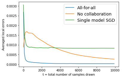
(a) Comparison of All-for-all with naive benchmarks

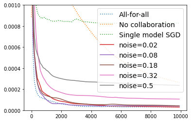
(b) Effect of noise in the estimation of bias parameters $b_{ij}$

Figure 1. All-for-all algorithm in practice

To test the robustness of our algorithms and our theory, we use in our experiments the mean estimation problem used in the strongly convex and smooth lower bound of Theorem 1: $\ell(x,\xi)=\frac{1}{2}{{\left\|x-\xi\right\|}}^{2}$, $x\in\mathbb{R}^{d}$ for $\xi$ a $d$-dimensional Bernoulli random variable. We use the time-adaptive version of Algorithm 1, and we place ourselves in the setting of Section A.4, where agent distributions are drawn from a distribution of distributions: for $N=100$ agents, we draw $(p_{i})_{1\leqslant i\leqslant N}$ i.i.d. uniformly distributed in $[0,1]$, and $p_{i}$ is the parameter of agent $i$’s Bernoulli variables. We draw $10^{3}$ samples for each agent, and we compute for $1\leqslant t\leqslant T$ the averaged local generalization errors (here the error from the mean), namely $\frac{1}{N}\sum_{i=1}^{N}\frac{1}{2}{{\left\|x_{i}^{t}-p_{i}\right\|}}^{2}$, where $x_{i}^{t}$ is the output of the algorithm after $t$ samples drawn. As expected and as illustrated in Figure 1(a), our all-for-all approach benefits from both no-collaboration (each agent locally estimating its mean $p_{i}$ with only its locally available samples, in orange in the graph) and single-model approaches (a fully centralized minimization of $\frac{1}{N}\sum_{i}f_{i}(x)$, in green in the graph), through both a convergence to the true mean, and a non-asymptotic acceleration. In Figure 1(b), we study the effect of noise on the estimation of bias parameters $b_{ij}$ (that here correspond to $b_{ij}=\frac{1}{2}(p_{i}-p_{j})^{2}$), by taking as inputs in algorithms $b_{ij}^{\rm noisy}=\frac{1}{2}(p_{i}+n_{i}-p_{j}-n_{j})^{2}$, where $n_{i}$ are i.i.d. uniformly distributed in $[-{\rm noise},{\rm noise}]$, for different noise values (Figure 1(b)). All-for-all algorithm appears to be quite robust to noise: for small noise amplitudes (0.02 and 0.08, and even 0.18), performances are not too degraded. For (abusively) large noise values (0.32 and 0.5), the non-asymptotic speedup is kept, with degraded asymptotic performances. Still, in the range of parameters considered, these perform better than no-collaboration and single model approaches.

Discussion and conclusion.

In this paper, we quantified in term of function biases ($b_{ij}$), stochastic gradient noise or amplitudes ($\sigma^{2}$ or $B^{2}$), target precision $\varepsilon>0$ and functions regularity parameters, the benefit of collaboration between agents for shared minimization using stochastic gradient algorithms. Our lower bound (Theorem 1) states that in the all-for-one setting, assumption parameters being fixed, no algorithm matches the performances of weighted gradient averagings in terms of sample optimality. Another lower bound (and corresponding upper-bounds) that would be worth investigating is: without any knowledge on biases $b_{ij}$, what is the worst case complexity of an algorithm that would thus need to learn who to learn with? We extended weighted gradient averagings to the all-for-all setting, technically more challenging, through the introduction of a related problem, simplifying the analysis of such algorithms.

The main limitation of our work lies in the assumption that upper-bounds on the biases $b_{ij}$ are known. We investigate in Section A scenarii in which this assumption is valid. Yet, as mentionned above, learning who to learn with and how is a challenging question worth tackling. Extending our work to model agnosticism together with data heterogeneity would require bias assumptions such as our distribution-based ones in Section A. Finally, fairness issues might be raised by our approaches in the all-for-all setting: we consider the average errors amongst agents and therefore do not ensure bounds on the supremum of all local errors. Still, incentives to collaborate and send gradients to other users are the hope of being helped back (matrix $W$ is symmetric in Algorithm 1).

Appendix A The Case of Collaborative Generalization Error Minimization (GEM)

In most of the related works and in this paper, the quantities equivalent to our bias assumptions are assumed to be known by the optimizer. Yet, while this assumption makes analyses possible, the knowledge of these quantities is a strong assumption. In this section, we provide settings and toy problems under which these assumptions are natural. We first begin by introducing distribution based distances between agents, in order to control gradient biases in the setting where functions are of the form (5) for a shared loss $\ell$ and local distributions $(\mathcal{D}_{i})_{i}$, for collaborative GEM. We then present two settings for this problem.

A.1. Distribution-based distances

In order to quantify the bias/variance tradeoff that appears when using stochastic gradients computed by other agents, we define the following notion of distance.

Definition 1.

For $\mathcal{H}$ a set of functions from $\Xi$ to $\mathbb{R}^{d}$ and $\mathcal{D},\mathcal{D}^{\prime}$ two probability distributions on $\Xi$, we define:

$$d_{\mathcal{H}}(\mathcal{D},\mathcal{D}^{\prime})=\sup_{h\in\mathcal{H}}{{\left\|\mathbb{E}\left[h(\xi)-h(\xi^{\prime})\right]\right\|}}\,,$$

where $\xi\sim\mathcal{D}$ and $\xi^{\prime}\sim\mathcal{D}^{\prime}$. $d_{\mathcal{H}}$ is a pseudo-distance on the set of probability measures on $\Xi$.

Some instances of these distances encompass:

1. For $\mathcal{H}=\mathcal{H}_{\rm Affine}$ the set of 1-Lipschitz affine functions, we have $d_{\mathcal{H}}(\mathcal{D},\mathcal{D}^{\prime})={{\left\|\mathbb{E}\left[\xi\right]-\mathbb{E}\left[\xi^{\prime}\right]\right\|}}$.

2. For $\mathcal{H}=\mathcal{H}_{\rm Lipschitz}$ the set of 1-Lipschitz functions on $\Xi$, we have $d_{\mathcal{H}}(\mathcal{D},\mathcal{D}^{\prime})=\mathcal{W}_{1}(\mathcal{D},\mathcal{D}^{\prime})$ the 1-Wasserstein distance (or EMD, earth mover distance).

3. For $\mathcal{H}=\mathcal{H}_{\rm Bounded}$ the set of of functions whose values lie in a space of diameter 1, we have $d_{\mathcal{H}}(\mathcal{D},\mathcal{D}^{\prime})=d_{\rm TV}(\mathcal{D},\mathcal{D}^{\prime})$ the total variation distance.

4. For $\mathcal{H}=\mathcal{H}_{\rm Loc.Bounded}$ defined as ${{\left\{h:\Xi\to\mathbb{R}^{d}\quad\text{s.t.}\quad\forall\xi\in\Xi,\,{\rm Diam}\big{(}h(\mathcal{B}(\xi,1)\cap\Xi)\big{)}\leqslant 1\right\}}}$, we also obtain the total variation distance.

The definition of $d_{\mathcal{H}}$ is motivated by the fact that, for fixed $x\in\mathcal{X}$ and $1\leqslant i,j\leqslant N$, we have:

$${{\left\|\nabla f_{i}(x)-\nabla f_{j}(x)\right\|}} ={{\left\|\mathbb{E}\left[\nabla_{x}\ell(x,\xi_{i})-\nabla_{x}\ell(x,\xi_{j})\right]\right\|}}$$

$$\leqslant d_{\mathcal{H}}(\mathcal{D}_{i},\mathcal{D}_{j})\,.$$

if $\big{(}\xi\in\Xi\mapsto\nabla_{x}\ell(x,\xi)\big{)}\in\mathcal{H}$ where $(\xi_{i},\xi_{j})\sim\mathcal{D}_{i}\times\mathcal{D}_{j}$.

We thus add a fourth bias assumptions to our list in Section 2, called distribution-based bias assumption: for some function set $\mathcal{H}$, for all $1\leqslant i,j\leqslant N$, for all $x\in\mathbb{R}^{d}$, $d_{\mathcal{H}}(\mathcal{D}_{i},\mathcal{D}_{j})\leqslant\hat{b}_{ij}$ for some non negative weights $\hat{b}$, and for all $x\in\mathbb{R}^{d}$, $\big{(}\xi\in\Xi\mapsto\nabla_{x}\ell(x,\xi)\big{)}\in\mathcal{H}$. This assumptions is verified in the following settings for mean estimation and regression.

1. For $\ell(x,\xi)=\frac{1}{2}(x-\xi)^{2}$ (mean estimation), distribution-based bias assumption holds for $\mathcal{H}_{\rm Affine}$, and the distance to consider is thus ${{\left\|\mathbb{E}\left[\xi_{i}\right]-\mathbb{E}\left[\xi_{j}\right]\right\|}}$.

2. For quadratic loss (linear regression) $\ell(x,\xi)=\frac{1}{2}(a^{\top}x-b)^{2}$ where $\xi=(aa^{\top},ba^{\top})$, we have $\mathcal{H}=D\mathcal{H}_{\rm Affine}$, where $D$ is the diameter of the space in which are iterates lie, and the distance to consider is thus a scaled 1-Wassertein distance between distributions

3. For logisic regression $\ell(x,\xi)=\log(1+e^{-ba^{\top}x})$ where $\xi=ba^{\top}$, we have $\mathcal{H}=(1+\frac{1}{e})\mathcal{H}_{\rm Lipschitz}$ and the distance to consider is thus the 1-Wassertein distance between distributions (scaled with a constant factor).

4. For the hinge loss $\ell(x,\xi)=\max(0,1-ba^{\top}x)$, for $\xi=ba^{\top}$ we have $\mathcal{H}=D\mathcal{H}_{\rm Bounded}$ where $D$ is the diameter of the space in which are iterates lie, and the distance to consider between distributions is thus a scaled total variation distance.

Thus, instead of controlling uniform concentration bounds on the gradients (under the GEM assumption, this can be done using anisotropic uniform concentration bounds, e.g. Even and Massoulie [2021]), one can leverage our bias assumptions by controlling distribution-based distances.

Proposition 1.

If for all $1\leqslant i,j\leqslant N$, $d_{\mathcal{H}}(\mathcal{D}_{i},\mathcal{D}_{j})\leqslant\hat{b}_{ij}$ (i.e. distribution-based bias assumption holds), then:

1. Bias assumption (B.1) holds for $b_{ij}=D^{\star}\hat{b}_{ij}$;

2. Bias assumption (B.2) holds for $\tilde{b}_{ij}=\hat{b}_{ij}^{2}$.

A.2. Lower-bounds (Theorem 1) in term of distribution based distances

Theorem 1 being formulated as IT-lower bounds for collaborative GEM, the distribution-based distances we introduced perfectly adapt to it. In fact, in the proof of the lower bounds, the distributions we build verify $d_{\mathcal{H}}(\mathcal{D}_{i},\mathcal{D}_{j})\leqslant b_{ij}$ if $\mathcal{H}\subset\mathcal{H}_{Loc.Bounded}$, so that the following directly holds.

Theorem 5.

Let $\varepsilon\in(0,1/16)$. Assume that the function set $\mathcal{H}$ satisfies:

$$\mathcal{H}_{\rm Affine}\subset\mathcal{H}\subset\mathcal{H}_{Loc.Bounded}\,,$$

and assume that either the synchronous or asynchronous oracle is used. Assume that $(b_{ij})$ verifies the triangle inequality $b_{ij}\leqslant b_{ik}+b_{kj}$ for all $1\leqslant i,j,k\leqslant N$. Let $\tilde{\mathbb{D}}(r,b,B)$ be the set $\mathbb{D}(r,b,B)$, but where the bias assumptions are replaced by the distribution-based bias assumption ($d_{\mathcal{H}}(\mathcal{D}_{i},\mathcal{D}_{j})\leqslant b_{ij}$), and similarly for $\tilde{\mathbb{D}}_{\mu=1/r^{2}}^{L=1/r^{2}}(r,b,\sigma)$. We have, for some constant $C>0$ independent of the problem and any $i\in\{1,\ldots,N\}$:

$$\inf_{\mathcal{M}\in\mathbb{M}}\!\sup_{((\mathcal{D}_{j})_{j},\ell)\in\tilde{\mathbb{D}}(r,b,B)}\!\!\!\!\!\!\mathcal{T}_{i}^{\varepsilon}\Big{(}\mathcal{M},\big{(}(\mathcal{D}_{j})_{j},\ell\big{)}\Big{)}\!\geqslant\!\frac{CB^{2}r^{2}N}{\varepsilon^{2}\mathcal{N}_{i}^{\varepsilon}(\frac{b}{4})}\,,$$

where $\mathcal{N}_{i}^{\varepsilon}(b)=\sum_{j}\mathds{1}_{\{b_{ij}\leqslant\varepsilon\}}$ is the number of agents $j$ verifying $b_{ij}\leqslant\varepsilon$. Under strong-convexity and smoothness assumptions for $\mu=L=1/r^{2}$, this bound becomes, for some constant $C^{\prime}>0$:

$$\inf_{\mathcal{M}\in\mathbb{M}}\!\sup_{((\mathcal{D}_{j})_{j},\ell)\in\tilde{\mathbb{D}}_{\mu=1/r^{2}}^{L=1/r^{2}}(r,b,\sigma)}\!\!\!\!\!\!\mathcal{T}_{i}^{\varepsilon}\Big{(}\mathcal{M},\big{(}(\mathcal{D}_{j})_{j},\ell\big{)}\Big{)}\geqslant\frac{C^{\prime}r^{2}\sigma^{2}N}{\varepsilon\mathcal{N}_{i}^{\varepsilon}(\frac{b}{4})}\,.$$

A.3. Weak supervision

We explicit in this section another paradigm in which the knowledge of some distribution-based bias assumptions is realistic, in a weakly supervised learning setting. More precisely, assume that the desired task is a classification or regression one: random variables $\xi$ are of the form $\xi=(\zeta,\beta)$ for some $\zeta\in Z\subset\mathbb{R}^{D_{1}}$ and some label $\beta\in\mathbb{R}^{D_{2}}$. For every agent $1\leqslant i\leqslant N$, let $\mathcal{D}_{i}^{\zeta}$ be the $\zeta$-marginal of $\mathcal{D}_{i}$. In our weakly supervised learning setting, we assume that there exists some (eventually random) function $\mathcal{L}$ that maps unlabelled data $\zeta$ to their labelled ones i.e. for some $\mathcal{L}:Z\to\Xi$, the random variable $\mathcal{L}(\zeta_{i})$ is of same law as $\xi_{i}\sim\mathcal{D}_{i}$ for $\zeta_{i}\sim\mathcal{D}_{i}^{\zeta}$. While many samples may be accessible and drawn from $\mathcal{D}_{i}^{\zeta}$ for every agent $1\leqslant i\leqslant N$, labelling data i.e. applying function $\mathcal{L}$ in order to recover samples of law $\mathcal{D}_{i}$ is assumed to be costly. For instance, applying $\mathcal{L}$ in medical data analysis could require the help form an expert (a radiologist, …).

Agents would benefit from computing distances between distributions $\mathcal{D}_{i}$ using marginals $\mathcal{D}_{i}^{\zeta}$: under mild assumptions on the function $\mathcal{L}$ (Lipschitzness with high probability, mainly), distances $d_{\mathcal{H}}(\mathcal{D}_{i},\mathcal{D}_{j})$ are upperbounded by distances between $\mathcal{D}_{i}^{\zeta}$ and $\mathcal{D}_{j}^{\zeta}$. Thus, in this setting, agents would benefit from collaborating: computing distribution-based distances would not require expert advices, while reducing the total number of expert calls required by reducing the number of samples needed to be drawn from each $\mathcal{D}_{i}$ through collaboration.

A.4. Infinitely-Many-Agents Limit and Geometrical Prior Knowledge

We introduce the infinitely-many-agents limit, by taking $N\to\infty$ with added structure on the problem below. This toy-problem illustrates a geometric structure under which the knowledge of distribution-based bias assumptions is realistic. Let $\mathcal{P}$ be a set of probability laws and $\Theta\subset\mathbb{R}^{p}$ be a set parameterizing $\mathcal{P}$ in the sense that $\mathcal{P}$ can be written as $\{\mathcal{D}_{\theta},\,\theta\in\Theta\}$ where $\mathcal{D}_{\theta},\,\theta\in\Theta$ are probability laws on $\Xi$. For all $1\leqslant i\leqslant N$, we assume that there exists $\theta_{1},\ldots,\theta_{N}\in\Theta$ such that $\mathcal{D}_{i}=\mathcal{D}_{\theta_{i}}$, and that the agents are drawn from a probability distribution with density $\nu$ on $\Theta$: $(\theta_{i})_{i}$ is a sequence of i.i.d. vectors sampled from $\Theta$ with density $\nu$.

This aims at modelling a geometric structure on the agents distributions: agents $i$ and $j$ such that $\theta_{i}$ and $\theta_{j}$ are nearby in the set $\Theta$ share similar distributions. We quantify this in the following way: there exists a continuous function $b:\Theta^{2}\to\mathbb{R}^{+}$ such that for any $(\theta,\theta^{\prime})\in\Theta^{2}$, $d_{\mathcal{H}}(\theta,\theta^{\prime})\leqslant b(\theta,\theta^{\prime})$. In sensor networks, $\Theta$ is some domain of $\mathbb{R}^{2}$ of $\mathbb{R}^{3}$, each agent is a sensor located at a physical position in $\Theta$, whose goal is to predict based on noisy local observations (e.g. temperature, pollution, …) that are space-continuous. More generally, if agents model a population (agent $i$ being an individual in the population) in some geographical location $\Theta\subset\mathcal{S}_{2}$ (sphere in $\mathbb{R}^{3}$) (ranging from cities, countries, continents, or the whole wide world), and if we are interested in speech-recognition models, a fair assumption is to have similar local distributions for nearby agents. The distribution $\nu$ is then the geographical density of agents.

The infinitely-many-agents limit is obtained by taking $N\to\infty$ with our geometric structure on the agents: we obtain a continuum of agents parameterized by $\theta\in\Theta$, with density $\nu$ on $\Theta$. For every $\theta\in\Theta$, we write:

$$f_{\theta}(x)=\mathbb{E}_{\xi\sim\mathcal{D}_{\theta}}[\ell(x,\xi)]\,,\quad x\in\mathcal{X}\,,$$

and we denote by $x_{\theta}^{\star}$ a minimizer over $\mathcal{X}$ of $f_{\theta}$. The algorithm and model we consider are defined as follows, inspired by Oracle 2.

Infinitely-many-agents oracle and algorithm At each time-step $t=1,2,...$: 1: An agent parameterized by $\theta_{t}\sim\nu$ is ‘awakened’, draws $\xi_{\theta_{t}}^{t}$ is drawn from data distribution $\mathcal{D}_{\theta_{t}}$ and computes a stochastic gradient $g_{t}=\nabla_{x}\ell(y_{t},\xi_{\theta_{t}}^{t})$. 2: Agents $\theta\in\Theta$ such that $w(\theta,\theta_{t})\leqslant s_{\varepsilon}$ for some fixed $s_{\varepsilon}$ receive $g_{t}$. 3: Upon reception of $g_{t}$, agents may update their local estimates.

At finite time-horizon $T>0$, only a finite number of agents may have ‘awakened’ and drawn (at most) one sample from their local distribution; yet, we aim at obtaining upper-bounds on the local generalization errors for all agents. Applying our AFO and AFA algorithms, under aditional assumptions, yields the following bounds.

Proposition 2.

Assume that $\nu$ is continuous on $\Theta$, and that for all $\theta,\theta^{\prime}\in\Theta$, we have $b(\theta,\theta^{\prime})\leqslant{{\left\|\theta-\theta^{\prime}\right\|}}^{q}$. Assume that assumption N.1 holds and that iterates lie in a space of diameter $D$.

1. All-for-one: let $\varepsilon>0$ and $\theta\in{\rm int}\ {A}$. There exists a procedure such that $T_{\varepsilon}(\theta)$ the time needed to reach a precision $\varepsilon$ for agent $\theta$ is upper-bounded by:

   $$T_{\varepsilon}(\theta)\leqslant\mathcal{O}_{\varepsilon\to 0}\left(B^{2}D^{2}\nu(\theta)\varepsilon^{-2-p/q}\right)\,.$$

2. All-for-all: for any $\varepsilon>0$, there exists a procedure making $T_{\varepsilon}$ oracle calls and answering $(x_{\theta})_{\theta}\in\mathcal{X}^{\Theta}$ such that:

   $$\int_{\Theta}\big{(}f_{\theta}(x_{\theta})-f_{\theta}(x_{\theta}^{\star})\big{)}\nu({\rm d}\theta)\leqslant\varepsilon\,,$$

   with

   $$T_{\varepsilon}\leqslant\mathcal{O}_{\varepsilon\to 0}\left(B^{2}D^{2}\varepsilon^{-2-p/q}\right)\,.$$

Proof.

For finite number of agents $N$, we have $\theta_{1},\ldots,\theta_{N}$ drawn i.i.d. from $\nu$. Using weighted gradient averagings and Theorem 2.1, we have for agent $i$, and denoting $\theta=\theta_{i}$:

$$T_{\varepsilon}(\theta)\leqslant 2B^{2}D^{2}\varepsilon^{-2}\frac{\mathcal{N}_{i}^{\varepsilon}(2b)}{N}\,.$$

Here, $\mathcal{N}_{i}^{\varepsilon}(2b)\leqslant|{{\left\{1\leqslant j\leqslant N\,:\,{{\left\|\theta-\theta_{j}\right\|}}\leqslant(\varepsilon/2)^{1/q}\right\}}}=\sum_{j=1}^{N}\mathds{1}_{{{\left\{{{\left\|\theta-\theta_{j}\right\|}}\leqslant(\varepsilon/2)^{1/q}\right\}}}}$. Using the strong law of large number, we have almost surely, as $N\to\infty$:

$$\frac{\mathcal{N}_{i}^{\varepsilon}(2b)}{N}\leqslant\int_{\mathcal{B}(\theta,(\varepsilon/2)^{1/q})}\nu(z){\rm d}z+o(1)\,.$$

Thus, for $N\to\infty$:

$$T_{\varepsilon}(\theta)\leqslant 2B^{2}D^{2}\int_{\mathcal{B}(\theta,(\varepsilon/2)^{1/q})}\nu(z){\rm d}z\,.$$

Then, making $\varepsilon\to 0$, we have $\int_{\mathcal{B}(\theta,(\varepsilon/2)^{1/q})}\nu(z){\rm d}z\sim_{\varepsilon\to 0}\nu(\theta){\rm Vol}(\mathcal{B}(\theta,(\varepsilon/2)^{1/q}))=\mathcal{O}\left(\nu(\theta)\varepsilon^{-p/q}\right)$ ($\nu$ is continuous). We thus have the result for $\theta$ such that $\nu(\theta)>0$ in the all-for-one setting.

In the all-for-all setting, we use Theorem 4.1 in for a finite number of agents, and we similarly use the strong law of large numbers as $N\to\infty$. ∎

Appendix B Proof of Lower-Bounds (Theorem 1 and Corollary 1)

B.1. General framework to prove lower bounds

The idea is that, when optimizing a function $f(x)=\mathbb{E}\left[\ell(x,\xi)\right]$ and finding a good approximation of a minimizer $x^{\star}$, we learn some information on the distribution $\mathcal{D}$ over which samples are drawn. In order to prove lower bounds, we construct a loss function $\ell$, and distributions $\mathcal{D}_{1}^{\alpha},\ldots,\mathcal{D}_{N}^{\alpha}$, where $\alpha$ is a random parameter. We argue that minimizing (in the all-for-all or all-for-one settings) the objective function up to a certain precision gives a good estimator (quantified) of the random seeds $\alpha$. Then, using Fano inequality, we bound the efficiency of such an estimator in terms of number of oracle calls, obtaining a lower bound on the sample complexity. This approach is inspired by Agarwal et al. [2012], who prove IT-lower bounds for stochastic gradient descent. We adapt their proof technique to the personalized and multi-agent setting.

Constructing difficult loss functions

For any two functions $f,g:\mathbb{R}^{d}\to\mathbb{R}$, we define the discrepancy measure $\rho(f,g)$ as:

$$\rho(f,g)=\inf_{x\in\mathbb{R}^{d}}\Big{\{}f(x)+g(x)-f(x_{f}^{*})-g(x_{f}^{*})\Big{\}}\,,$$

which is a pseudo metrics. Now, for a finite set $\mathcal{V}$ of parameters, let $\mathcal{G}(\delta)={{\left\{g_{\alpha}^{\delta}\,,\,\alpha\in\mathcal{V}\right\}}}$ be a set of functions indexed by $\mathcal{V}$, that depend on $\delta$ (fixed in the set). The dependency of each $g_{\alpha}\in\mathcal{G}(\delta)$ is left implicit in the following subsections. We define:

$$\psi(\delta)=\inf_{f,g\in\mathcal{G}(\delta)}\rho(f,g)\,.$$

Minimizing is Bernoulli parameters identification

The two following lemmas justify that optimizing a function $g_{\alpha}\in\mathcal{G}(\delta)$ to a precision of order $\psi(\delta)$ is more difficult than estimating the parameter $\alpha$.

Lemma 1 (Agarwal et al. [2012]).

For any $x\in\mathbb{R}^{d}$, there can be at most one function $g_{\alpha}$ in $\mathcal{G}(\delta)$ such that:

$$g_{\alpha}(x)-\inf_{\mathbb{R}^{d}}g_{\alpha}<\frac{\psi(\delta)}{3}\,.$$

Lemma 2 (Agarwal et al. [2012]).

Assume that for some fixed but unknown $\alpha\in\mathcal{V}$ there exists a method $\mathcal{M}_{T}$ based on the data $\phi=\{X_{1},...,X_{T}\}$ that returns $x^{T}$ (function of $\phi$) satisfying an error of:

$$\mathbb{E}\left[g_{\alpha}(x^{T})-\min_{x\in\mathbb{R}^{d}}g_{\alpha}(x)\right]<\frac{\psi(\delta)}{9}\,,$$

where the mean is taken over the randomness of both the oracle $\Phi$, the method $\mathcal{M}_{T}$ and $\alpha\in\mathcal{V}$ if random. Then, there exists a hypothesis test $\hat{\alpha}:\phi\to\mathcal{V}$ such that:

$$\max_{\alpha\in\mathcal{V}}\mathbb{P}_{\phi}\big{(}\hat{\alpha}\neq\alpha\big{)}\leqslant\frac{1}{3}\,.$$

Suppose now that the parameter $\alpha$ in the previous Lemma is chosen uniformly at random in $\mathcal{V}$. Let $\hat{\alpha}:\phi\to\mathcal{V}$ be a hypothesis test estimating $\alpha$. By Fano inequality [Cover and Thomas, 2005], we have:

$$\mathbb{P}\big{(}\hat{\alpha}\neq\alpha)\geqslant 1-\frac{I\big{(}\phi,\alpha\big{)}+\ln(2)}{|\mathcal{V}|}\,,$$ (9)

where $I\big{(}\phi,\alpha\big{)}$ is the mutual information between $\phi$ and $\alpha$, that we need to upper-bound. Combining Fano inequality with Lemmas 1 and 2, fixing a target error $\varepsilon=\psi(\delta)$, we obtain a lower bound on the sample complexity $T_{\varepsilon}$:

$$\frac{1}{3}\geqslant\mathbb{P}_{\phi}\big{(}\hat{\alpha}\neq\alpha\big{)}\geqslant 1-\frac{I\big{(}\phi_{T_{\varepsilon}},\alpha\big{)}+\ln(2)}{|\mathcal{V}|}\,,$$

where $\phi_{T_{\varepsilon}}$ is the information contained in $T_{\varepsilon}$ oracle calls. If we have an equality of the form $I\big{(}\phi_{T_{\varepsilon}},\alpha\big{)}=T_{\varepsilon}I\big{(}\phi_{1},\alpha\big{)}$, this gives:

$$T_{\varepsilon}\geqslant\frac{\frac{2}{3}|\mathcal{V}|-\ln(2)}{I(\phi_{1},\alpha)}\,.$$ (10)

Playing with the different parameters $\delta,\alpha,\mathcal{V}$ gives lower bounds in our all-for-one settings. We refer the interested reader to Chapter 2 in Cover and Thomas [2005] for Fano inequality and mutual information.

B.2. Applying this in the all-for-one setting, first part of Theorem 1

We first prove the lower bounds in the case of the asynchronous oracle (one data item sampled from personal distribution at each iteration).

We define the loss $\ell:\mathbb{R}^{d}\times\Xi$ where $\Xi\subset\mathbb{R}^{d}$ and $\delta>0$:

$$\forall(x,\xi)\in\mathcal{X}\times\Xi\,,\quad\ell(x,\xi)=\frac{1}{d}\sum_{i=1}^{d}\Big{[}\xi f_{i}^{+}(x)+(1-\xi)f_{i}^{-}(x)-\delta x_{i}\Big{]}\,,$$

where

$$f_{i}^{+}(x)=|x_{i}+1/2|\,\quad f_{i}^{-}(x)=|x_{i}-1/2|\,.$$

Now, for any $\alpha\in\{-1,1\}^{d}$, $\delta\in[0,1/2]$ being fixed, we define:

$$g_{\alpha}(x)=\frac{1}{d}\sum_{i=1}^{d}\Big{[}\big{(}\frac{1}{2}+\alpha_{i}\delta\big{)}f_{i}^{+}(x)+\big{(}\frac{1}{2}-\alpha_{i}\delta\big{)}f_{i}^{-}(x)-\delta x_{i}\Big{]}\,.$$ (11)

For simplicity, assume that $r^{2}=d$ and $B^{2}=1$. Let $\delta>0$ a free parameter. Let $\mathcal{V}=\{\alpha^{1},\ldots,\alpha^{K}\}\subset\{-1,1\}^{d}$ be a subset of the hypercube such that for all $k\neq l$,

$$\frac{1}{2}\sum_{i=1}^{d}|\alpha_{i}^{k}-\alpha_{i}^{l}|\geqslant\frac{d}{4}\,,$$

i.e. $\mathcal{V}$ is a $d/4$-packing of the hypercube. We assume that $-\mathds{1}$ ($d$-dimensional vector with $-1$ at all its entries) is not in $\mathcal{V}$ and that for all $\alpha\in\mathcal{V}$, $\frac{1}{2}\sum_{i=1}^{d}|\alpha_{i}+1|\geqslant\frac{d}{4}$. We know that we can set $|\mathcal{V}|\geqslant(2/\sqrt{e})^{d/2}$. Without loss of generality, we prove a lower bound in the case where the agent that desires to minimize its local function is indexed by $1$. For any $i=1,\ldots,N$, let $\mathcal{D}_{i}$ be the probability distribution on $\{0,1\}^{d}$ of the following random variable:

$${\rm Ber}\big{(}\frac{1}{2}+\delta_{i}\alpha_{k}\big{)}\epsilon_{k}\quad\text{where}\quad\delta_{i}=(\delta-b_{i1})^{+}\,,\\$$

where $s^{+}=\max(0,s)$ for $s\in\mathbb{R}$, $k$ is taken uniformly at random in $\{1,\ldots,d\}$, $(\epsilon_{k})$ is the canonical basis of $\mathbb{R}^{d}$, and ${Ber}(p)$ is a Bernoulli random variable, independent of $k$.

The function $f_{1}(x)=\mathbb{E}\left[\ell(x,\xi_{1})\right]$ for $\xi_{1}\sim\mathcal{D}_{1}$ verifies $f_{1}=g_{\alpha}$ for $g_{\alpha}$ defined in (11). For our fixed $\delta>0$ and any $\alpha,\beta\in\mathcal{V}$, $g_{\alpha}$ is minimized at $x^{\alpha}=-\alpha/2$ and we have:

$$g_{\alpha}(x^{\alpha})=\frac{1}{d}\sum_{k=1}^{d}\frac{1-\delta\alpha_{k}}{2}\,.$$

The discrepancies thus write as:

$$\rho(g_{\alpha},g_{\beta})=\frac{\delta}{d}\sum_{k=1}^{d}|\alpha_{k}-\beta_{k}|\,,$$

so that $\psi(\delta)\geqslant\delta/4$. Each $g_{\alpha}$ is minimized for $x^{\alpha}=-\alpha/2\in\mathcal{B}_{\infty}(0,1/2)\subset\mathcal{B}(0,\sqrt{d}/2)\subset\mathcal{B}(x^{0},r)$ for $x^{0}=0$ (where $\mathcal{B}_{\infty}$ denotes a ball for the infinity norm): we are in the case $r=\sqrt{d}$.

We now bound the quantities $f_{i}(x_{j}^{\star})-f_{i}(x_{i}^{\star})$. For any $i=1,\ldots,N$, we have $x_{i}^{\star}=x^{\alpha}=-\alpha/2$ if $\delta_{i}\geqslant\delta/2$, and $x_{i}^{\star}=\mathds{1}/2$ otherwise. For $1\leqslant i,j\leqslant N$, if both $\delta_{i}\geqslant\delta/2$ and $\delta_{j}\geqslant\delta/2$, then $x_{i}^{\star}=x_{j}^{\star}=x^{\alpha}$, and $f_{i}(x_{j}^{\star})-f_{i}(x_{i}^{\star})=0$. Similarly, if both $\delta_{i}<\delta/2$ and $\delta_{j}<\delta/2$, $x_{i}^{\star}=x_{j}^{\star}=\mathds{1}/2$ and $f_{i}(x_{j}^{\star})-f_{i}(x_{i}^{\star})=0$. If $\delta_{i}\geqslant\delta/2$ and $\delta_{j}<\delta/2$, then

$$f_{i}(x_{j}^{\star})-f_{i}(x_{i}^{\star}) =f_{i}(\mathds{1}/2)-f_{i}(x^{\alpha})$$

$$=\frac{1}{d}\sum_{k=1}^{d}\frac{|\alpha_{k}-1|}{2}(2\delta_{i}-\delta)$$

$$\leqslant 2\delta_{i}-\delta$$

$$\leqslant 2(\delta_{i}-\delta_{j})\,.$$

Since $\delta_{i}-\delta_{j}\leqslant b_{ij}/2$ using 1-Lipschitzness of the positive value and the triangle inequality verified by the vector $b$, we have $f_{i}(x_{j}^{\star})-f_{i}(x_{i}^{\star})\leqslant b_{ij}$. If $\delta_{i}<\delta/2$ and $\delta_{j}>\delta/2$, we similarly have $f_{i}(x_{j}^{\star})-f_{i}(x_{i}^{\star})\leqslant\frac{1}{d}\sum_{k=1}^{d}\frac{|\alpha_{k}-1|}{2}(\delta-2\delta_{i})\leqslant b_{ij}$.

Since the functions $f_{i}$ are differentiable at all points where $x_{k}\neq 1/2,-1/2$, bounding ${{\left\|\nabla f_{i}(x)-\nabla f_{j}(x)\right\|}}^{2}$ at the points where $f_{i}$ and $f_{j}$ are differentiable is enough to have (B.2). For $x_{k}<-1/2$, we have $\nabla_{k}f_{i}(x)=\nabla_{k}f_{j}(x)=-1-\delta$ and $\nabla_{k}f_{i}(x)=\nabla_{k}f_{j}(x)=1-\delta$ for $x_{k}>1/2$. For $-1/2<x_{k}<1/2$, we have $\nabla_{k}f_{i}(x)-\nabla_{k}f_{j}(x)-2(\delta_{i}-\delta_{j})\alpha_{k}$, so that ${{\left\|\nabla f_{i}(x)-\nabla f_{j}(x)\right\|}}^{2}\leqslant 4(\delta_{i}-\delta_{j})^{2}\leqslant b_{ij}^{2}/d$ at all points where $f_{i}$ and $f_{j}$ are differentiable. The gradients scale with $r$, hence the dependency in $r$ (we recall that $r^{2}=d$ in our case).

The mutual information $I(\phi_{T},\alpha)$ writes as:

$$I(\phi_{T},\alpha) =TI(\phi_{1},\alpha)$$

$$=\frac{T}{dN}\sum_{k=1}^{d}\sum_{i=1}^{N}I\left({\rm Ber}\big{(}\frac{1}{2}+\mathds{1}_{b_{1i}\leqslant\delta}\alpha_{k}\delta_{i}\big{)},\alpha_{k}\right)$$

$$\leqslant\frac{C_{1}T}{N}\sum_{i=1}^{N}\mathds{1}_{b_{1i}<\delta}\delta_{i}^{2}$$

$$=\frac{C_{1}T\mathcal{N}_{1}^{\delta}(b)}{N}\delta^{2}\,,$$

for some numerical constant $C>0$ independent of the problem. Using Equation (10) then leads to, for $\varepsilon=\psi(\delta)$:

$$T_{\varepsilon}\geqslant C\frac{dN}{\varepsilon^{2}\mathcal{N}_{1}^{\varepsilon}(4b)}\,,$$ (12)

where $C>0$ is a numerical constant independent of the problem.

Equation (12) is obtained for the choice of loss function and distributions defined above, and the functions defined are in $\mathbb{D}(r,b,B)$ for $r=\sqrt{d}$, the fixed weights $b$, and $B^{2}=1$. Assumption $\mathcal{B}_{\infty}(0,1/2)\subset\mathcal{B}(0,\sqrt{d}/2)\subset\mathcal{X}$ is in Theorem 1 the assumption that ${{\left\|x^{0}-x_{i}^{\star}\right\|}}\leqslant r$. In order to obtain a dependency in $r>0$, one simply has to consider the loss $(x,\xi)\mapsto\ell(\frac{\sqrt{d}}{2r}x,\xi)$. In order to obtain the dependency in $B^{2}$, we need to modify the distribution, and take $\mathcal{D}_{i}^{\prime}={\rm Ber}(1/B^{2})B^{2}\mathcal{D}_{i}$. In this case, we have a noise amplitude of order $B^{2}$ instead of order $1$, and a factor $1/B^{2}$ appears in the mutual information.

The proof naturally extends to Oracle 1: the mutual information is just $N$ times bigger in that case.

In terms of function distances $d_{\mathcal{H}}$ under the assumptions on $\mathcal{H}$ of Theorem 5, we have, since the distributions are Bernoulli:

$$d_{\mathcal{H}}(\mathcal{D}_{i},\mathcal{D}_{j})\leqslant|\delta_{i}-\delta_{j}|\leqslant b_{ij}.$$

We thus proved the first part of Theorem 1.

B.3. Proof of the strongly convex and smooth lower bound: second part of Theorem 1

Let

$$\ell(x,\xi)=\frac{1}{2}{{\left\|x-\xi\right\|}}^{2}\,$$

for $x,\xi\in\mathbb{R}^{d}$ and, for fixed $\delta>0$ and any $\alpha\in\{-1,1\}^{d}$:

$$g_{\alpha}(x)=\frac{1}{2d}\sum_{k=1}^{d}\Big{(}x_{k}^{2}+1-2\big{(}\frac{1}{2}+\alpha_{k}\delta)x_{k}\Big{)}\quad,x\in\mathcal{X}\,.$$

We keep the same notations as last subsection ($\psi(\delta),\rho$). We have:

$$\rho(g_{\alpha},g_{\beta})=\frac{\delta^{2}}{d}\sum_{k=1}^{d}|\alpha_{k}-\beta_{k}|\,.$$

Similarly to last subsection, this leads to $\psi(\delta)\geqslant\delta^{2}/4$ since $\mathcal{V}$ is a $d/4$-packing of the hypercube.

We keep the same distributions $\mathcal{D}_{1},...,\mathcal{D}_{N}$ as last subsection, replacing $\delta_{i}$ by $\delta_{i}=(\delta-\sqrt{b_{1i}})^{+}$. Agent 1 is still the one that wants to minimize its local generalization error. The mutual information is thus:

$$I(\phi_{T},\alpha)\leqslant\frac{C_{1}T\mathcal{N}_{1}^{\delta}(\sqrt{b})}{N}\delta^{2}\,.$$

Setting the target precision as $\varepsilon=\delta^{2}/4$, we obtain:

$$T_{\varepsilon}\geqslant C^{\prime}\frac{dN}{\varepsilon\mathcal{N}_{1}^{\varepsilon}(4b)}\,.$$

The loss function and distributions built verify our regularity assumptions for $\mu=1/d$, $L=1/d$, noise $\sigma^{2}\leqslant 1$.

We verify that for all $1\leqslant j,k\leqslant N$, we have $f_{j}(x_{k}^{\star})-f_{j}(x_{j}^{\star})\leqslant b_{kj}$. We first notice that $x_{j}^{\star}=\frac{1}{d}\big{(}\frac{1}{2}+\delta_{j}\alpha_{l}\big{)}_{1\leqslant l\leqslant d}$, so that:

$$f_{j}(x_{k}^{\star})-f_{j}(x_{j}^{\star}) =\frac{1}{d}{{\left\|x_{j}^{\star}-x_{k}^{\star}\right\|}}^{2}$$

$$=(\delta_{i}-\delta_{k})^{2}$$

$$\leqslant(\sqrt{b_{1j}}-\sqrt{b_{1k}})^{2}$$

$$\leqslant|b_{1j}-b_{1k}|$$

$$\leqslant b_{jk}\,,$$

since the weights $b$ verify the triangle inequality. Under the assumptions of Theorem 5 on $\mathcal{H}$, we have, in terms of distribution-based distances:

$$d_{\mathcal{H}}(\mathcal{D}_{i},\mathcal{D}_{j})\leqslant|\delta_{i}-\delta_{j}|\leqslant\sqrt{b_{ij}}\,.$$

The minimum of each $g_{\alpha}$ is attained at $x^{\alpha}=\frac{1}{2}+\delta\alpha$, we thus need to assume as in last subsection that $r$ is of order $\sqrt{d}$, and a rescaling leads to the dependency in $r$. The dependency in $\sigma^{2}$ is obtained as in last subsection.

Appendix C All-for-all lower bound

Theorem 1 immediately yields a Corollary providing lower bounds for the all-to-all problem:

Corollary 1.

Let $\varepsilon>0$, $b$ verifying the triangle inequality, $B>0,r>0$. Assume that there exists a method $\mathcal{M}$ and some $T>0$ such that, for all $((\mathcal{D}_{j})_{j},\ell)\in\mathbb{D}(r,b,B)$, $\mathcal{M}$ returns $(x_{1},\ldots,x_{N})$ verifying:

$$\frac{1}{N}\sum_{i=1}^{N}f_{i}(x_{i})-f_{i}(x_{i}^{\star})\leqslant\varepsilon\,.$$

where $T$ is the number of stochastic gradients sampled from all agents. Then we have:

$$T\geqslant\frac{Cr^{2}B^{2}}{N^{2}\varepsilon^{2}}\sum_{i=1}^{N}\frac{1}{\mathcal{N}_{i}^{\varepsilon}(\frac{b}{4N})}\,.$$

Replacing $\mathbb{D}(r,b,B)$ by $\mathbb{D}_{\mu=1/r^{2}}^{L=1/r^{2}}(r,b,\sigma)$, we have:

$$T\geqslant\frac{C^{\prime}r^{2}\sigma^{2}}{N\varepsilon}\sum_{i=1}^{N}\frac{1}{\mathcal{N}_{i}^{\varepsilon}(\frac{b}{4N})}\,.$$

Appendix D All-for-one upper-bounds

We provide the following relaxation of bias assumption B.2, a generalization of classical function dissimilarities assumptions Karimireddy et al. [2020], Chayti et al. [2021] to our setting.

1. For all $1\leqslant i\leqslant N$, for any stochastic vector $\lambda\in\mathbb{R}^{N}$ (non-negative entries that sum to 1), and for all $x\in\mathbb{R}^{d}$, where $g_{\lambda}(x)=\sum_{j=1}^{N}\lambda_{j}\nabla f_{j}(x)$:

   $${{\left\|\nabla f_{i}(x)-g_{\lambda}(x)\right\|}}^{2}\leqslant m{{\left\|g_{\lambda}(x)\right\|}}^{2}+\sum_{j=1}^{N}\lambda_{j}\tilde{b}_{ij}\,.$$ (13)

In a similar setting ($N$ agents with heterogeneous functions), Karimireddy et al. [2020], Deng et al. [2020], Chayti et al. [2021] assume that for a fixed agent (or for any agent) $i$, ${{\left\|\nabla f_{i}(x)-\nabla\bar{f}(x)\right\|}}^{2}\leqslant m{{\left\|\nabla\bar{f}(x)\right\|}}^{2}+\zeta^{2}$ (or similar assumptions) where $\bar{f}$ is the mean of all functions. (B.2) is the simplest relaxation of this to the more general setting where all agents want to minimize their local function, while (B.3) is a relaxation that keeps the less-restrictive first term for some $m\geqslant 0$.

We prove the following intermediate result.

Theorem 6 (WGA).

Let $(x^{k})_{k\geqslant 0}$ be generated with (6), for some fixed stochastic vector $\lambda\in\mathbb{R}^{N}$, stepsize $\eta>0$. Let $1\leqslant i\leqslant N$ fixed. Let $b\in{\mathbb{R}^{+}}^{N\times N}$. Denote $F_{i}^{k}=f_{i}(x^{k})-f_{i}(x_{i}^{\star})$.

1. Use the asynchronous oracle. Assume that for all $k\geqslant 0$ and $i$, ${{\left\|x^{k}-x_{i}^{\star}\right\|}}\leqslant D$ for some $D>0$. If $f_{i}$ is convex, noise assumption (N.1) holds for some $B>0$ and bias assumption (B.2) holds for $\tilde{b}=(b/D)^{2}$, for any $K>0$ and for $\eta=\sqrt{\frac{D^{2}}{2KNB^{2}\sum_{j=1}^{N}\lambda_{j}^{2}}}$:

   $$\mathbb{E}\left[\frac{1}{K}\sum_{0\leqslant k<K}F_{i}^{k}\right] \leqslant\sqrt{\frac{2D^{2}B^{2}}{\frac{K}{N}}\sum_{j=1}^{N}\lambda_{j}^{2}}+\sum_{1\leqslant j\leqslant N}\lambda_{j}b_{ij}\,.$$

2. Use the synchronous oracle. Assume that all $f_{j}$ are $\mu$-strongly convex and $L$-smooth (denote $\kappa=L/\mu$), satisfy noise assumption N.2 for some $\sigma>0$, that one of bias assumptions (B.2) or (B.3) holds for $\tilde{b}=\mu b$ (and any $m\geqslant 0$). For any $K>0$ and $\eta=\min(1/(2L),\frac{1}{\mu K}\ln(\frac{F_{\lambda}^{0}\mu^{2}K}{L\sigma^{2}}\sum_{j}\lambda_{j}^{2}))$ where $F_{\lambda}^{0}=\sum_{j}\lambda_{j}(f_{j}(x^{0})-f_{j}(x_{j}^{\star}))$, we have:

   $$\mathbb{E}\left[F_{i}^{K}\right]\leqslant 2(m+1)\kappa\left(F_{\lambda}^{0}e^{-\frac{K}{2\kappa}}+\tilde{\mathcal{O}}\left(\frac{L\sigma^{2}}{\mu^{2}K}\sum_{1\leqslant j\leqslant N}\lambda_{j}^{2}\right)\right)+\sum_{1\leqslant j\leqslant N}\lambda_{j}b_{ij}\,.$$

This leads to a more general sample complexity in Setting 2, where we can use (B.3).

Theorem 7.

Let $\varepsilon>0$, and set $\lambda_{j}=\frac{\mathds{1}_{{{\left\{b_{ij}<\varepsilon/2\right\}}}}}{\mathcal{N}_{i}^{\varepsilon}(2b)}$, $\mathcal{N}_{i}^{\varepsilon}$ being defined in Theorem 1. Generate $(x^{k})_{k}$ using (6).

1. Under Setting 1. Assume that for all $k\geqslant 0$ and $i$, ${{\left\|x^{k}-x_{i}^{\star}\right\|}}\leqslant D$ for some $D>0$ and bias assumption (B.2) holds for $\tilde{b}=(b/D)^{2}$. For $K=T_{\varepsilon}$ and for $\eta=\sqrt{\frac{D^{2}}{2KNB^{2}\sum_{j=1}^{N}\lambda_{j}^{2}}}$, we have $\mathbb{E}\left[\frac{1}{K}\sum_{0\leqslant k<K}f_{i}(x^{k})-f_{i}(x_{i}^{\star})\right]\leqslant\varepsilon$ using a total number $T_{\varepsilon}$ of stochastic gradients from all agents of:

   $$T_{\varepsilon}\leqslant\frac{4D^{2}B^{2}}{\varepsilon^{2}}\frac{N}{\mathcal{N}_{i}^{\varepsilon}(2b)}\,.$$

2. Under Setting 2. Denote $\kappa=L/\mu$, assume that one of bias assumptions (B.2) or (B.3) holds for $\tilde{b}=\mu b$ (and any $m\geqslant 0$). For $K=T_{\varepsilon}/N$ and $\eta=\min(1/(2L),\frac{1}{\mu K}\ln(\frac{F_{\lambda}^{0}\mu^{2}K}{L\sigma^{2}}\sum_{j}\lambda_{j}^{2}))$ where $F_{\lambda}^{0}=\sum_{j}\lambda_{j}(f_{j}(x^{0})-f_{j}(x_{j}^{\star}))$, we have $\mathbb{E}\left[f_{i}(x^{K})-f_{i}(x_{i}^{\star})\right]\leqslant\varepsilon$ using a total number $T_{\varepsilon}$ of stochastic gradients from all agents of:

   $$T_{\varepsilon}\leqslant\tilde{\mathcal{O}}\left(\frac{(m+1)\kappa^{2}\sigma^{2}}{\mu\varepsilon}\frac{N}{\mathcal{N}_{i}^{\varepsilon}(2b)}\right)\,,$$

   and of

   $$T_{\varepsilon}\leqslant\tilde{\mathcal{O}}\left(\frac{\kappa\sigma^{2}}{\mu\varepsilon}\frac{N}{\mathcal{N}_{i}^{\varepsilon}(2b)}\right)\,,$$

   if $m\leqslant 1/2$.

In Theorem 6.b upper-bound, the first term is the optimization term, and vanishes exponentially quickly in front of the second and third ones (if they are non null), and is not reminiscent of our personalized problem. The second is the noise term (referred to as the statistical term), while the third is a bias term, making appear as advertised in the introduction a bias-variance trade-off. In Theorem 6.a, only the statistical and the bias terms are present. In both cases, a right choice of $\lambda_{ij}$ matches the lower bound of Theorem 1 in terms of sample complexity, for $\varepsilon>0$ small enough such that the optimization term vanishes in front of the statistical one. In Theorem 6.a, $D$ plays the role of $r$ in the lower bound (and can be more restrictive). Parameters $\mu,L$ in Theorem 6.b can take any value, while they are fixed in our lower bounds (with $\kappa=1$).

For the two proofs below, we write

$$g_{\lambda}^{k}(x)=\sum_{j=1}^{N}\lambda_{j}G^{k}(x)_{j}\,.$$

D.1. Proof of Theorem 6.a

Assume first that the $f_{j}$ are differentiable. Observe first that under noise assumption (N.1) and with the asynchronous oracle:

$$\mathbb{E}\left[{{\left\|g_{\lambda}^{k}(x)\right\|}}^{2}\right]\leqslant\sum_{j=1}^{N}N\lambda_{j}^{2}B^{2}\,,\quad x\in\mathbb{R}^{d}\,.$$

We now proceed following classical SGD analysis, but with biased gradients here. Denote $e_{i}^{k}=\mathbb{E}\left[{{\left\|x^{k}-x_{i}^{\star}\right\|}}^{2}\right]$. We have:

$$e_{i}^{k+1} =e_{i}^{k}-2\mathbb{E}\left[\langle\sum_{j=1}^{N}\lambda_{j}\nabla f_{j}(x^{k}),x^{k}-x_{i}^{\star}\rangle\right]+\eta^{2}\mathbb{E}\left[{{\left\|g_{\lambda}^{k}\right\|}}(x^{k})\right]$$

$$\leqslant e_{i}^{k}-2\eta\mathbb{E}\left[\langle\nabla f(x^{k}),x^{k}-x_{i}^{\star}\rangle\right]+\boldsymbol{2\eta\mathbb{E}\left[\langle\nabla f(x^{k})-\sum_{j=1}^{N}\lambda_{j}\nabla f_{j}(x^{k}),x^{k}-x_{i}^{\star}\rangle\right]}+\eta^{2}\sum_{j=1}^{N}N\lambda_{j}^{2}B^{2}\,,$$

where the bold term is the bias term, that we bound by $D\sum_{j}\lambda_{j}\sqrt{\tilde{b}_{ij}}=\sum_{j}\lambda_{j}b_{ij}$ using bias assumption (2) and $\tilde{b}_{ij}=(b_{ij}/D)^{2}$. Then, since $-2\eta\mathbb{E}\left[\langle\nabla f(x^{k}),x^{k}-x_{i}^{\star}\rangle\right]\leqslant-2\eta\mathbb{E}F_{i}^{k}$, we have, summing the above inequality for $1\leqslant k\leqslant K$:

$$\sum_{k=0}^{K-1}F_{i}^{k}\leqslant\frac{e_{i}^{0}}{2\eta}+K\frac{\eta}{2}NB^{2}\sum_{j=1}^{N}\lambda_{j}^{2}+K\sum_{j=1}^{N}\lambda_{j}b_{ij}\,.$$

We obtain the desired result by dividing by $K$ and for the choice of $\eta$ as in Theorem 3.a. In the case where we have access to subdifferentials only, the proof stays identical (as in Lemma 6).

D.2. Proof of Theorem 6.b

Denoting $f^{\lambda}(x)=\sum_{j=1}^{N}\lambda_{j}f_{j}(x)$, observe that $f^{\lambda}$ is $\mu$-strongly convex and $L$-smooth, and for all $x\in\mathbb{R}^{d}$, under the synchronous oracle and noise assumption (N.2):

$$\mathbb{E}\left[g_{\lambda}^{k}(x)\right]=\nabla f^{\lambda}(x)\,,$$ (14)

$$\mathbb{E}\left[{{\left\|g_{\lambda}^{k}(x)-\nabla f^{\lambda}(x)\right\|}}^{2}\right]\leqslant\sigma^{2}\sum_{j=1}^{N}\lambda_{j}^{2}\,.$$

Applying Lemma 4 (SGD under strong convexity and smoothness assumptions), we have, where $x^{\lambda}$ minimizes $f^{\lambda}$:

$$f^{\lambda}(x^{k})-f^{\lambda}(x^{\lambda})\leqslant F_{\lambda}^{0}e^{-\frac{k}{2\kappa}}+\tilde{\mathcal{O}}\left(\frac{L\sigma^{2}}{\mu^{2}k}\sum_{1\leqslant j\leqslant N}\lambda_{j}^{2}\right)\,.$$

Then, under either bias assumption (B.2) or (B.3), we have:

$${{\left\|\nabla f_{i}(x^{k})\right\|}}^{2} \leqslant 2{{\left\|\nabla f_{i}(x^{k})-\nabla f^{\lambda}(x^{k})\right\|}}^{2}+2{{\left\|\nabla f^{\lambda}(x^{k})\right\|}}^{2}$$

$$\leqslant 2(m{{\left\|\nabla f^{\lambda}(x^{k})\right\|}}^{2}+\sum_{j=1}^{N}\lambda_{ij}\tilde{b}_{ij})+2{{\left\|\nabla f^{\lambda}(x^{k})\right\|}}^{2}$$

$$\leqslant 2\sum_{j=1}^{N}\lambda_{ij}\tilde{b}_{ij}+4L(m+1)(f^{\lambda}(x^{k})-f^{\lambda}(x^{\lambda}))\,.$$

We conclude using $f_{i}(x^{k})-f_{i}(x_{i}^{\star})\leqslant\frac{1}{2\mu}{{\left\|\nabla f_{i}(x^{k})\right\|}}^{2}$ and $\tilde{b}_{ij}=\mu b_{ij}$.

This result is valid under any $m\geqslant 0$, and gives the first part of Theorem 7.2. If $m\leqslant 1/2$, one can use Theorem 1 in Chayti et al. [2021] with the set of agents $j$ such that $b_{ij}\leqslant\varepsilon$, agent $0$ is agent $i$, with $\alpha=1/\mathcal{N}_{i}^{\varepsilon}(2b)$, to obtain the sample complexity without the $\kappa$ factor.

Appendix E All-for-all upper-bounds

We first begin with the following simple lemma.

Lemma 3.

If $\Lambda$ is a stochastic matrix and if bias assumption (B.1) holds ($f_{i}(x_{j}^{\star})-f_{i}(x_{i}^{\star})\leqslant b_{ij}$ for all $1\leqslant i,j\leqslant N$):

$$f^{\Lambda}(x^{\Lambda})-\bar{f}(x^{\star})\leqslant\frac{1}{N}\sum_{1\leqslant i,j\leqslant N}\lambda_{ij}b_{ij}\,.$$

Proof.

Writing the optimality of $x^{\Lambda}$ gives:

$$f^{\Lambda}(x^{\Lambda}) \leqslant f^{\Lambda}(x^{\star})$$

$$=\frac{1}{N}\sum_{i}f_{i}(\sum_{j}\lambda_{ij}x_{j}^{\star})$$

$$\leqslant\frac{1}{N}\sum_{1\leqslant i,j\leqslant N}\lambda_{ij}f_{i}(x_{j}^{\star})\,,$$

where we used convexity of each $f_{i}$. Then, subtracting $\bar{f}(x^{\star})$ and using stochasticity of $\Lambda$:

$$f^{\Lambda}(x^{\Lambda})-\bar{f}(x^{\star})\leqslant\frac{1}{N}\sum_{1\leqslant i,j\leqslant N}\lambda_{ij}(f_{i}(x_{j}^{\star})-f_{i}(x_{i}^{\star}))\,.$$

∎

E.1. Proof of Theorem 3.a

Using Lemma 3 and the proof sketch ($f^{\Lambda}(y^{k})=\bar{f}(x^{k})$ and the bias variance decomposition):

$$\bar{f}(x^{k})-\bar{f}(x^{\star})\leqslant f^{\Lambda}(y^{k})-f^{\Lambda}(x^{\Lambda})+\frac{1}{N}\sum_{1\leqslant i,j\leqslant N}\lambda_{ij}b_{ij}\,,$$

where $(y^{k})$ is generated using simple SGD on $f^{\Lambda}$:

$$y^{k+1}=y^{k}-\eta\nabla G^{k}_{\Lambda}(y^{k})\,,$$

where

$$G^{k}_{\Lambda}(y)=\big{(}\lambda_{i_{k}j}g_{i_{k}}^{k}((\Lambda y^{k})_{i_{k}}))\big{)}_{1\leqslant j\leqslant N}\,.$$

$f^{\Lambda}$ is convex, and we have under noise assumption (N.1) for the asynchronous oracle, under differentiable assumptions:

$$\mathbb{E}\left[G^{k}_{\Lambda}(y)\right]=\nabla f^{\Lambda}(y)\,,$$

$$\mathbb{E}\left[{{\left\|G^{k}_{\Lambda}(y)\right\|}}^{2}\right]\leqslant\frac{B^{2}}{N}\sum_{1\leqslant i,j\leqslant N}\lambda_{ij}^{2}\,.$$

If we only have subdifferentials, we still have $\mathbb{E}\left[G^{k}_{\Lambda}(y)\right]\in\partial f^{\Lambda}(y)$. Using Lemma 6 (SGD under these assumptions), we obtain the desired result.

E.2. Proof of Theorem 3.b

Under noise assumption (N.2) and for the synchronous oracle, we stil have:

$$y^{k+1}=y^{k}-\eta\nabla G^{k}_{\Lambda}(y^{k})\,,$$

for

$$G^{k}_{\Lambda}(y)=\frac{1}{N}\big{(}\sum_{i=1}^{N}\lambda_{ij}g_{i}^{k}((\Lambda y^{k})_{i}))\big{)}_{1\leqslant j\leqslant N}\,,$$

that verifies:

$$\mathbb{E}\left[G^{k}_{\Lambda}(y)\right]=\nabla f^{\Lambda}(y)\,,$$

$$\mathbb{E}\left[{{\left\|G^{k}_{\Lambda}(y)-\nabla f^{\lambda}(y)\right\|}}^{2}\right]\leqslant\frac{\sigma^{2}}{N^{2}}\sum_{1\leqslant i,j\leqslant N}\lambda_{ij}^{2}\,.$$

The function $f^{\Lambda}$ is however not necessarily strongly convex. However, since $\nabla^{2}f^{\Lambda}(y)=\Lambda^{\top}\nabla^{2}\bar{f}(\Lambda y)\Lambda$ and $\bar{f}$ is $L/N$-smooth and $\mu/N$-strongly convex, $f^{\Lambda}$ is $L/N$-relatively smooth and $\mu/N$-relatively strongly convex [Bauschke et al., 2017] with respect to $\frac{1}{2}{{\left\|y\right\|}}_{W}^{2}=\frac{1}{2}y^{\top}Wy$. Note also that the spectral radius of $W$ is $1$, since $\Lambda$ is stochastic. Instead of using stochastic Bregman gradient descent (e.g. Dragomir et al. [2021]), we use Lemma 4: classical SGD that naturally generalizes to relative smoothness and strong convexity assumptions, when the mirror map is quadratic.

E.3. Time-adaptive variant

Algorithm 2 All-for-all algorithm: Time-adaptive variant

1:  Stepsizes $(\eta_{k})_{k\geqslant 0}$, matrixes $(W^{(k)})_{k\geqslant 0}$

2:  Initialization $x_{1}^{0}=\ldots=x_{N}^{0}\in\mathbb{R}^{d}$

3:  for $k=0,1,2,\ldots$ do

4:     Agents $j\in S^{k}$ (activated agents) compute stochastic gradients $g_{j}^{k}(x_{j}^{k})$ and broadcast it to all agents $i$ such that $W^{(k)}_{ij}>0$.

5:     For $i=1,\ldots,N$, update

$$x_{i}^{k+1}=x_{i}^{k}-\eta_{k}\sum_{j\in S^{k}}W^{(k)}_{ij}g^{k}_{j}(x^{k}_{j})$$

6:  end for

Proposition 3 (Time-adaptive all-for-all).

Assume that the same assumptions as in Theorem 3.a hold. For any $\varepsilon>0$, denote $\Lambda_{\varepsilon}=(\frac{\mathds{1}_{2b_{ij}\leqslant\varepsilon}}{\mathcal{N}_{i}^{\varepsilon}(2b)}$, $K_{\varepsilon}=\frac{4D^{2}B^{2}}{\varepsilon^{2}}\sum_{i=1}^{N}\frac{1}{\mathcal{N}_{i}^{\varepsilon}(2b)}$ and $\eta(\varepsilon)=\frac{2ND^{2}}{K_{\varepsilon}B^{2}\sum_{i}1/\mathcal{N}_{i}^{\varepsilon}(2b)}$. For any $k\geqslant 0$, there exists $p_{k}\geqslant 0$ such that $\sum_{q=0}^{p_{k}-1}T_{2^{-q}}\leqslant k<\sum_{q=0}^{p_{k}}T_{2^{-q}}$, and choose:

$$\eta_{k}=\eta(2^{-p_{k}})\,,\quad W^{(k)}=\Lambda_{2^{-p_{k}}}\Lambda_{2^{-p_{k}}}^{\top}\,.$$

Then, for any $\varepsilon>0$, the iterates generated by Algorithm 2 reach averaged precision $\varepsilon$ for a number of data item sampled from personal distribution of:

$$T_{\varepsilon}\leqslant\frac{16D^{2}B^{2}}{\varepsilon^{2}}\sum_{i=1}^{N}\frac{1}{\mathcal{N}_{i}^{\varepsilon}(2b)}\,,$$

Similarly, under strong-convexity and smoothness assumptions as in Theorem 3.b, one would obtain the corresponding sample complexity, up to a factor 2.

E.4. Setting 2 under $\mu=0$

Theorem 8 (All-for-all, convex case).

Let $K>0$, $\eta>0$, and $W$ a symmetric non-negative random matrix of the form $W=\Lambda\Lambda^{\top}$ for some stochastic matrix $\Lambda=(\lambda_{ij})_{1\leqslant i,j\leqslant N}$. Let $(x_{i}^{k})_{k\geqslant 0,1\leqslant i\leqslant N}$ be generated with Algorithm 1. Assume that bias assumption (B.1) holds for some $(b_{ij})$. Under Setting 2, for $\mu=0$ (convex case), if $\eta=\frac{N^{3/2}D}{\sigma\sqrt{\sum_{i,j}\lambda_{ij}^{2}}}\wedge\frac{N}{2L}$, where ${{\left\|x_{i}^{0}-x_{i}^{\Lambda}\right\|}}\leqslant D$ for all $i$, we have:

$$\mathbb{E}\left[F^{K}\right] \leqslant\frac{2LD^{2}}{K}+\sqrt{\frac{2D^{2}\sigma^{2}}{KN}\sum_{1\leqslant i,j\leqslant N}\lambda_{ij}^{2}}+\sum_{1\leqslant i,j\leqslant N}\lambda_{ij}b_{ij}\,.\vspace{-5pt}$$

Consequently, for $\varepsilon>0$, and a choice of $W=\Lambda\Lambda^{\top}$ for $\lambda_{ij}=\frac{\mathds{1}_{{\left\{b_{ij}<\varepsilon/2\right\}}}}{\mathcal{N}_{i}^{\varepsilon}(2b)}$ and under the same assumptions, the all-for-all algorithm reaches $\mathbb{E}\left[F^{K}\right]\leqslant\varepsilon$ for a total number $T_{\varepsilon}$ of data item sampled from personal distributions of:

$$T_{\varepsilon}\leqslant\max\left(\frac{8D^{2}\sigma^{2}}{\varepsilon^{2}}\sum_{i=1}^{N}\frac{1}{\mathcal{N}_{i}^{\varepsilon}(2b)},\,\frac{4NLD^{2}}{\varepsilon}\right)$$

Proof.

Combining Lemma 5 with the noise variance and regularity parameters of $F^{\Lambda}$. ∎

Appendix F Stochastic Optimization Toolbox

F.1. SGD under strongly convex and smooth assumptions

Lemma 4 (SGD, s.c. and smooth).

Define ${{\left\|x\right\|}}_{A}^{2}=x^{\top}Ax$ for some non-negative and symmetric matrix $A$. Let $f:\mathcal{X}\to\mathbb{R}$ $\mu$-relatively strongly convex and $L$-relatively smooth with respect to $\frac{1}{2}{{\left\|x\right\|}}_{A}^{2}$. Let $(f_{t},g_{t})_{t\geqslant 0}$ be first order oracle calls such that for all $t\geqslant 0$:

$$\forall x\in\mathcal{X}\,,\quad\left\{\begin{aligned} &\mathbb{E}\left[f_{t}(x)\right]=f(x)\,,\\ &\mathbb{E}\left[g_{t}(x)\right]=\nabla f(x)\,,\\ &\mathbb{E}\left[{{\left\|g_{t}(x)-\nabla f(x)\right\|}}^{2}\right]\leqslant\sigma^{2}\,,\end{aligned}\right.$$

for some $\sigma>0$. Let $L_{A}$ be the largest eigenvalue of $A$, and assume that $L_{A}\leqslant 1$ (our result generalizes to any $L_{A}$). Let $(x_{t})_{t\geqslant 0}$ be generated with:

$$\forall t\geqslant 0\,,\quad x^{t+1}=x^{t}-\eta g_{t}(x^{t})\,,$$

for a fixed stepsize $\frac{1}{2L}\geqslant\eta>0$, and assume that all the iterates lie in $\mathcal{X}$. Assume that $f$ is minimized over $\mathcal{X}$ at some interior point $x^{\star}$. We have for any $T>0$:

$$\mathbb{E}\left[f(x^{T})-f(x^{\star})\right]\leqslant e^{-\eta\mu T}\big{(}f(x^{0})-f(x^{\star})\big{)}+\frac{\eta L\sigma^{2}}{\mu}\,.$$

For fixed $T>0$, setting $\eta=\min\big{(}1/(2L),\frac{1}{\mu T}\ln(\frac{f_{0}\mu^{2}T}{L\sigma^{2}})\big{)}$ gives:

$$\mathbb{E}\left[f(x^{T})-f(x^{\star})\right]\leqslant e^{-\frac{\mu}{2L}T}\big{(}f(x^{0})-f(x^{\star})\big{)}+\frac{L\sigma^{2}}{\mu^{2}T}\ln\big{(}\frac{f_{0}\mu^{2}T}{L\sigma^{2}}\big{)}\,.$$

Thus, for fixed target precision $\varepsilon>0$, using stepsize $\eta_{\varepsilon}=\min\left(\frac{\mu\varepsilon}{2L\sigma^{2}},\frac{1}{2L}\right)$ and setting $T_{\varepsilon}=\lceil\ln\big{(}\varepsilon^{-1}(f(x^{0})-f(x^{\star}))\big{)}\frac{1}{\eta_{\varepsilon}\mu}\rceil$, we have:

$$f\left(\frac{1}{T_{\varepsilon}}\sum_{t<T_{\varepsilon}}x^{t}\right)-f(x^{\star})\leqslant\varepsilon\,,$$

with a number of oracle calls

$$T_{\varepsilon}\leqslant\max\left(\frac{2L\sigma^{2}}{\varepsilon\mu^{2}},\frac{2L}{\mu}\right)\ln\big{(}\varepsilon^{-1}(f(x^{0})-f(x^{\star}))\big{)}\,.$$

Proof.

For some $t\geqslant 0$, denoting $f_{t}=\mathbb{E}\left[f(x^{t+1})-f(x^{\star})\right]$, using relative smoothness, unbiasedness of the stochastic gradients and then relative strong convexity:

$$f_{t+1}-f_{t} \leqslant-\eta\mathbb{E}\left[{{\left\|\nabla f(x^{t})\right\|}}^{2}\right]+\frac{\eta^{2}L}{2}\mathbb{E}\left[{{\left\|g_{t}\right\|}}_{A}^{2}\right]$$

$$\leqslant-\eta\mathbb{E}\left[{{\left\|\nabla f(x^{t})\right\|}}^{2}\right]+\frac{\eta^{2}LL_{A}}{2}\mathbb{E}\left[{{\left\|g_{t}\right\|}}^{2}\right]$$

$$\leqslant-\eta\left(1-\frac{\eta LL_{A}}{2}\right)\mathbb{E}\left[{{\left\|\nabla f(x^{t})\right\|}}^{2}\right]+\frac{\eta^{2}LL_{A}\sigma^{2}}{2}\,.$$

Using relative strong convexity of $f$, we have:

$${{\left\|\nabla f(x^{t})\right\|}}^{2} \geqslant\frac{1}{L_{A}}{{\left\|\nabla f(x^{t})\right\|}}_{A}^{2}$$

$$\leqslant\frac{2\mu}{L_{A}}f_{t}\,,$$

yielding, for $\eta<1/(LL_{A})$

$$f_{t+1}-f_{t}\leqslant-2\eta\frac{\mu}{L_{A}}f_{t}+\frac{\eta^{2}LL_{A}\sigma^{2}}{2}\,.$$

Then, for some $T>0$ and since $L_{A}\leqslant 1$, sum the above inequality multiplied by $\left(1-\eta\mu\right)^{-t-1}$:

$$\sum_{0\leqslant t\leqslant T-1}\left(1-\eta\mu\right)^{-t-1}f_{t+1}-\left(1-\eta\mu\right)^{-t}f_{t} \leqslant\frac{\eta^{2}L\sigma^{2}}{2}\sum_{0\leqslant t\leqslant T-1}\left(1-\eta\mu\right)^{-t-1}$$

$$\leqslant\frac{\eta^{2}L\sigma^{2}}{2}\frac{\left(1-\eta\mu\right)^{-t-1}}{\eta\mu}\,,$$

leading to the desired result. ∎

F.2. SGD under smoothness and convexity assumptions

Lemma 5 (SGD, convex and smooth).

Let $f:\mathcal{X}\to\mathbb{R}$ convex and $L$-smooth. Let $(f_{t},g_{t})_{t\geqslant 0}$ be first order oracle calls such that for all $t\geqslant 0$:

$$\forall x\in\mathcal{X}\,,\quad\left\{\begin{aligned} &\mathbb{E}\left[f_{t}(x)\right]=f(x)\,,\\ &\mathbb{E}\left[g_{t}(x)\right]=\nabla f(x)\,,\\ &\mathbb{E}\left[{{\left\|g_{t}(x)-\nabla f(x)\right\|}}^{2}\right]\leqslant\sigma^{2}\,,\end{aligned}\right.$$

for some $\sigma>0$. Let $(x_{t})_{t\geqslant 0}$ be generated with:

$$\forall t\geqslant 0\,,\quad x^{t+1}=x^{t}-\eta g_{t}(x^{t})\,,$$

for a fixed stepsize $\frac{1}{2L}\geqslant\eta>0$, and assume that all the iterates lie in $\mathcal{X}$. Assume that $f$ is minimized over $\mathcal{X}$ at some interior point $x^{\star}$. Denote, for $T>0$, $\bar{x}^{T}=\frac{1}{T}\sum_{0\leqslant t<T}x^{t}$. We have for any $T>0$:

$$\mathbb{E}\left[f(\bar{x}^{T})-f(x^{\star})\right]\leqslant\frac{{{\left\|x^{0}-x^{\star}\right\|}}^{2}}{\eta T}+\eta\sigma^{2}\,.$$

For fixed $T>0$, setting $\eta=\min\Big{(}1/(2L)),\frac{{{\left\|x^{0}-x^{\star}\right\|}}}{\sigma\sqrt{T}}\Big{)}$ gives:

$$\mathbb{E}\left[f(x^{T})-f(x^{\star})\right]\leqslant\frac{2{{\left\|x^{0}-x^{\star}\right\|}}\sigma}{\sqrt{T}}+\frac{2L{{\left\|x^{0}-x^{\star}\right\|}}^{2}}{T}\,.$$

Thus, for fixed target precision $\varepsilon>0$, we have:

$$f\left(\frac{1}{T_{\varepsilon}}\sum_{t<T_{\varepsilon}}x^{t}\right)-f(x^{\star})\leqslant\varepsilon\,,$$

with a number of oracle calls

$$T_{\varepsilon}\leqslant 4{{\left\|x^{0}-x^{\star}\right\|}}^{2}\big{(}4\sigma^{2}\varepsilon^{-2}+L\varepsilon^{-1}\big{)}\,.$$

Proof.

Denote $e_{t}=\mathbb{E}\left[{{\left\|x^{t}-x^{\star}\right\|}}^{2}\right]$. We have:

$$e_{t+1}-e_{t} \leqslant-2\eta\langle\nabla f(x^{t}),x^{t}-x^{\star}\rangle+\eta^{2}\mathbb{E}\left[{{\left\|g_{t}^{2}\right\|}}\right]$$

$$\leqslant-2\eta f_{t}+\eta^{2}(\mathbb{E}\left[{{\left\|\nabla f(x^{t})\right\|}}^{2}\right]+\sigma^{2})$$

$$\leqslant-2\eta(1-L\eta)f_{t}+\eta^{2}\sigma^{2}$$

$$\leqslant-\eta f_{t}+\eta^{2}\sigma^{2}\,,$$

where we used convexity and smoothness assumptions. Then, summing:

$$\sum_{t<T}f_{t}\leqslant\frac{e_{0}-e_{T}}{\eta}+T\eta\sigma^{2}\,,$$

leading to the desired result. ∎

F.3. SGD under convex assumptions

Lemma 6 (SGD, convex).

Let $f:\mathcal{X}\to\mathbb{R}$ convex. Let $(f_{t},g_{t})_{t\geqslant 0}$ be first order oracle calls such that for all $t\geqslant 0$:

$$\forall x\in\mathcal{X}\,,\quad\left\{\begin{aligned} &\mathbb{E}\left[f_{t}(x)\right]=f(x)\,,\\ &\mathbb{E}\left[g_{t}(x)\right]\in\partial f(x)\,,\\ &\mathbb{E}\left[{{\left\|g_{t}(x)\right\|}}^{2}\right]\leqslant B^{2}\,,\end{aligned}\right.$$

for some $B>0$. For $p_{\mathcal{X}}$ the projection on the convex set $\mathcal{X}$, let $(x_{t})_{t\geqslant 0}$ be generated with:

$$\forall t\geqslant 0\,,\quad x^{t+1}=p_{\mathcal{X}}\left(x^{t}-\eta g_{t}(x^{t})\right)\,,$$

for a fixed stepsize $\eta>0$. Assume that $f$ is minimized over $\mathcal{X}$ at some interior point $x^{\star}$. We have for any $T>0$ and for $\eta=\sqrt{\frac{2D^{2}}{B^{2}T}}$ for $D^{2}\geqslant{{\left\|x^{0}-x^{\star}\right\|}}^{2}$:

$$f\left(\frac{1}{T}\sum_{t<T}x^{t}\right)-f(x^{\star})\leqslant\sqrt{\frac{2}{T}}BD\,.$$

Thus, for fixed target precision $\varepsilon>0$, setting $T_{\varepsilon}=\lceil 2\varepsilon^{-2}B^{2}D^{2}\rceil$ and using stepsize $\eta_{\varepsilon}=\frac{\sqrt{2}\varepsilon}{B^{2}}$, we have:

$$f\left(\frac{1}{T_{\varepsilon}}\sum_{t<T_{\varepsilon}}x^{t}\right)-f(x^{\star})\leqslant\varepsilon\,.$$

Proof.

For any $y\in\mathcal{X}$, using properties of $p_{\mathcal{X}}$:

$${{\left\|x^{t+1}-y\right\|}}^{2} ={{\left\|p_{\mathcal{X}}\left(x^{t}-\eta g_{t}(x^{t})\right)-y\right\|}}^{2}$$

$$\leqslant{{\left\|x^{t}-\eta g_{t}(x^{t})-y\right\|}}^{2}$$

$$={{\left\|x^{t}-y\right\|}}^{2}+\eta^{2}{{\left\|g_{t}(x^{t})^{2}\right\|}}-2\eta\langle g_{t}(x^{t}),x^{t}-y\rangle\,.$$

Taking the mean and $y=x^{\star}$, with $e_{t}=\mathbb{E}\left[{{\left\|x^{t}-x^{\star}\right\|}}^{2}\right]$ and $f_{t}=\mathbb{E}\left[f(x^{t})-f(x^{\star})\right]$:

$$e_{t+1} \leqslant e_{t}+\eta^{2}B^{2}-2\eta\langle\nabla f(x^{t}),x^{t}-y\rangle$$

$$\leqslant e_{t}+\eta^{2}B^{2}-2\eta f_{t}\,,$$

where we used convexity of $f$. Thus, $f_{t}\leqslant\frac{e_{t}-e_{t+1}}{2\eta}+\frac{\eta B^{2}}{2}$, and by summing this inequality for $0\leqslant t<T$:

$$\sum_{t<T}f_{t}\leqslant\frac{e_{0}-e_{T}}{2\eta}+\frac{\eta TB^{2}}{2}\leqslant\frac{e_{0}}{\eta}+\frac{\eta TB^{2}}{2}\,.$$

Thus, for $\eta=\sqrt{\frac{2e_{0}}{B^{2}T}}$, we have the result using convexity of $f$. ∎

References

• Agarwal et al. (2012) Alekh Agarwal, Peter L. Bartlett, Pradeep Ravikumar, and Martin J. Wainwright. Information-theoretic lower bounds on the oracle complexity of stochastic convex optimization. IEEE Transactions on Information Theory, 58(5):3235–3249, 2012.
• Bauschke et al. (2017) Heinz H. Bauschke, Jérôme Bolte, and Marc Teboulle. A descent lemma beyond lipschitz gradient continuity: First-order methods revisited and applications. Mathematics of Operations Research, 42(2):330–348, 2017.
• Beaussart et al. (2021) Martin Beaussart, Felix Grimberg, Mary-Anne Hartley, and Martin Jaggi. WAFFLE: Weighted Averaging for Personalized Federated Learning. arXiv:2110.06978 [cs], October 2021.
• Bellet et al. (2018) Aurélien Bellet, Rachid Guerraoui, Mahsa Taziki, and Marc Tommasi. Personalized and private peer-to-peer machine learning. In Proceedings of the Twenty-First International Conference on Artificial Intelligence and Statistics, volume 84 of Proceedings of Machine Learning Research, pages 473–481, 2018.
• Bottou et al. (2018) Léon Bottou, Frank E. Curtis, and Jorge Nocedal. Optimization methods for large-scale machine learning. SIAM Review, 60(2):223–311, January 2018.
• Chayti et al. (2021) El Mahdi Chayti, Sai Praneeth Karimireddy, Sebastian U. Stich, Nicolas Flammarion, and Martin Jaggi. Linear speedup in personalized collaborative learning, 2021.
• Cheng et al. (2021) Gary Cheng, Karan Chadha, and John Duchi. Fine-tuning is Fine in Federated Learning. arXiv:2108.07313 [cs, math, stat], August 2021.
• Cover and Thomas (2005) Thomas M. Cover and Joy A. Thomas. Elements of Information Theory. Wiley, April 2005.
• Deng et al. (2020) Yuyang Deng, Mohammad Mahdi Kamani, and Mehrdad Mahdavi. Adaptive Personalized Federated Learning. arXiv:2003.13461 [cs, stat], November 2020. arXiv: 2003.13461.
• Donahue and Kleinberg (2021a) Kate Donahue and Jon Kleinberg. Model-sharing games: Analyzing federated learning under voluntary participation. Proceedings of the AAAI Conference on Artificial Intelligence, 35(6):5303–5311, May 2021a.
• Donahue and Kleinberg (2021b) Kate Donahue and Jon Kleinberg. Optimality and stability in federated learning: A game-theoretic approach. In Advances in Neural Information Processing Systems, 2021b.
• Dragomir et al. (2021) Radu Alexandru Dragomir, Mathieu Even, and Hadrien Hendrikx. Fast stochastic bregman gradient methods: Sharp analysis and variance reduction. In Proceedings of the 38th International Conference on Machine Learning, volume 139 of Proceedings of Machine Learning Research, pages 2815–2825. PMLR, 18–24 Jul 2021.
• Duchi and Rogers (2019) John Duchi and Ryan Rogers. Lower bounds for locally private estimation via communication complexity. In Proceedings of the Thirty-Second Conference on Learning Theory, volume 99 of Proceedings of Machine Learning Research, pages 1161–1191, Phoenix, USA, June 2019. PMLR.
• Duchi and Wainwright (2013) John C. Duchi and Martin J. Wainwright. Distance-based and continuum fano inequalities with applications to statistical estimation. 2013.
• Even and Massoulie (2021) Mathieu Even and Laurent Massoulie. Concentration of non-isotropic random tensors with applications to learning and empirical risk minimization. In Mikhail Belkin and Samory Kpotufe, editors, Proceedings of Thirty Fourth Conference on Learning Theory, volume 134 of Proceedings of Machine Learning Research, pages 1847–1886. PMLR, 15–19 Aug 2021. URL https://proceedings.mlr.press/v134/even21a.html.
• Even et al. (2021) Mathieu Even, Raphaël Berthier, Francis Bach, Nicolas Flammarion, Hadrien Hendrikx, Pierre Gaillard, Laurent Massoulié, and Adrien Taylor. Continuized accelerations of deterministic and stochastic gradient descents, and of gossip algorithms. In A. Beygelzimer, Y. Dauphin, P. Liang, and J. Wortman Vaughan, editors, Advances in Neural Information Processing Systems, 2021. URL https://openreview.net/forum?id=bGfDnD7xo-v.
• Fallah et al. (2020) Alireza Fallah, Aryan Mokhtari, and Asuman Ozdaglar. Personalized Federated Learning with Theoretical Guarantees: A Model-Agnostic Meta-Learning Approach. Advances in Neural Information Processing Systems, 33:3557–3568, 2020.
• Grimberg et al. (2021) Felix Grimberg, Mary-Anne Hartley, Sai P. Karimireddy, and Martin Jaggi. Optimal Model Averaging: Towards Personalized Collaborative Learning. arXiv:2110.12946 [cs, stat], October 2021. arXiv: 2110.12946.
• Hanzely et al. (2020) Filip Hanzely, Slavomír Hanzely, Samuel Horváth, and Peter Richtarik. Lower Bounds and Optimal Algorithms for Personalized Federated Learning. In Advances in Neural Information Processing Systems, volume 33, pages 2304–2315. Curran Associates, Inc., 2020.
• Kairouz et al. (2019) Peter Kairouz, H. Brendan McMahan, Brendan Avent, Aurélien Bellet, Mehdi Bennis, Arjun Nitin Bhagoji, Keith Bonawitz, Zachary Charles, Graham Cormode, Rachel Cummings, Rafael G. L. D’Oliveira, Salim El Rouayheb, David Evans, Josh Gardner, Zachary Garrett, Adrià Gascón, Badih Ghazi, Phillip B. Gibbons, Marco Gruteser, Zaid Harchaoui, Chaoyang He, Lie He, Zhouyuan Huo, Ben Hutchinson, Justin Hsu, Martin Jaggi, Tara Javidi, Gauri Joshi, Mikhail Khodak, Jakub Konečný, Aleksandra Korolova, Farinaz Koushanfar, Sanmi Koyejo, Tancrède Lepoint, Yang Liu, Prateek Mittal, Mehryar Mohri, Richard Nock, Ayfer Özgür, Rasmus Pagh, Mariana Raykova, Hang Qi, Daniel Ramage, Ramesh Raskar, Dawn Song, Weikang Song, Sebastian U. Stich, Ziteng Sun, Ananda Theertha Suresh, Florian Tramèr, Praneeth Vepakomma, Jianyu Wang, Li Xiong, Zheng Xu, Qiang Yang, Felix X. Yu, Han Yu, and Sen Zhao. Advances and Open Problems in Federated Learning. arXiv:1912.04977 [cs, stat], December 2019. arXiv: 1912.04977.
• Karimireddy et al. (2020) Sai Praneeth Karimireddy, Satyen Kale, Mehryar Mohri, Sashank Reddi, Sebastian Stich, and Ananda Theertha Suresh. SCAFFOLD: Stochastic Controlled Averaging for Federated Learning. In Proceedings of the 37th International Conference on Machine Learning, pages 5132–5143. PMLR, November 2020. ISSN: 2640-3498.
• Khodak et al. (2019) Mikhail Khodak, Maria-Florina F Balcan, and Ameet S Talwalkar. Adaptive Gradient-Based Meta-Learning Methods. In Advances in Neural Information Processing Systems, volume 32. Curran Associates, Inc., 2019.
• Konečný et al. (2016) Jakub Konečný, H. Brendan McMahan, Daniel Ramage, and Peter Richtárik. Federated Optimization: Distributed Machine Learning for On-Device Intelligence. arXiv:1610.02527 [cs], October 2016. arXiv: 1610.02527.
• Kulkarni et al. (2020) Viraj Kulkarni, Milind Kulkarni, and Aniruddha Pant. Survey of Personalization Techniques for Federated Learning. arXiv:2003.08673 [cs, stat], March 2020. arXiv: 2003.08673.
• Li et al. (2020) Tian Li, Maziar Sanjabi, Ahmad Beirami, and Virginia Smith. Fair resource allocation in federated learning. In International Conference on Learning Representations, 2020.
• Mansour et al. (2020) Yishay Mansour, Mehryar Mohri, Jae Ro, and Ananda Theertha Suresh. Three Approaches for Personalization with Applications to Federated Learning. arXiv:2002.10619 [cs, stat], July 2020. arXiv: 2002.10619.
• McMahan et al. (2017) Brendan McMahan, Eider Moore, Daniel Ramage, Seth Hampson, and Blaise Aguera y Arcas. Communication-Efficient Learning of Deep Networks from Decentralized Data. In Aarti Singh and Jerry Zhu, editors, Proceedings of the 20th International Conference on Artificial Intelligence and Statistics, volume 54 of Proceedings of Machine Learning Research, pages 1273–1282. PMLR, 20–22 Apr 2017.
• Mohri et al. (2019) Mehryar Mohri, Gary Sivek, and Ananda Theertha Suresh. Agnostic Federated Learning. In Proceedings of the 36th International Conference on Machine Learning, pages 4615–4625. PMLR, May 2019. ISSN: 2640-3498.
• Nedich et al. (2018) Angelia Nedich, Alex Olshevsky, and Michael G. Rabbat. Network topology and communication-computation tradeoffs in decentralized optimization. Proceedings of the IEEE, 106(5):953–976, May 2018.
• Scaman et al. (2019) Kevin Scaman, Francis Bach, Sébastien Bubeck, Yin Tat Lee, and Laurent Massoulié. Optimal convergence rates for convex distributed optimization in networks. Journal of Machine Learning Research, 20(159):1–31, 2019.
• T. Dinh et al. (2020) Canh T. Dinh, Nguyen Tran, and Josh Nguyen. Personalized Federated Learning with Moreau Envelopes. Advances in Neural Information Processing Systems, 33:21394–21405, 2020.
• Tripuraneni et al. (2020) Nilesh Tripuraneni, Michael Jordan, and Chi Jin. On the theory of transfer learning: The importance of task diversity. In H. Larochelle, M. Ranzato, R. Hadsell, M. F. Balcan, and H. Lin, editors, Advances in Neural Information Processing Systems, volume 33, pages 7852–7862. Curran Associates, Inc., 2020.
• Vanhaesebrouck et al. (2017) Paul Vanhaesebrouck, Aurélien Bellet, and Marc Tommasi. Decentralized Collaborative Learning of Personalized Models over Networks. In Aarti Singh and Jerry Zhu, editors, Proceedings of the 20th International Conference on Artificial Intelligence and Statistics, volume 54 of Proceedings of Machine Learning Research, pages 509–517. PMLR, 20–22 Apr 2017.
• Wang et al. (2019) Kangkang Wang, Rajiv Mathews, Chloé Kiddon, Hubert Eichner, Françoise Beaufays, and Daniel Ramage. Federated Evaluation of On-device Personalization. arXiv:1910.10252 [cs, stat], October 2019. arXiv: 1910.10252.
• Yu et al. (2021) Tao Yu, Eugene Bagdasaryan, and Vitaly Shmatikov. Salvaging Federated Learning by Local Adaptation. arXiv:2002.04758 [cs, stat], October 2021. arXiv: 2002.04758.
• Zhang et al. (2013) Yuchen Zhang, John Duchi, Michael I Jordan, and Martin J Wainwright. Information-theoretic lower bounds for distributed statistical estimation with communication constraints. In C. J. C. Burges, L. Bottou, M. Welling, Z. Ghahramani, and K. Q. Weinberger, editors, Advances in Neural Information Processing Systems, volume 26. Curran Associates, Inc., 2013.