Multi-species count transformation models

Abstract

By extending single-species distribution models, multi-species distribution models and joint species distribution models are able to describe the relationship between environmental variables and a community of species. It is also possible to model either the marginal distribution of each species (multi-species models) in the community or their joint distribution (joint species models) under certain assumptions, but a model describing both entities simultaneously has not been available. We propose a novel model that allows description of both the joint distribution of multiple species and models for the marginal single-species distributions within the framework of multivariate transformation models. Model parameters can be estimated from abundance data by two approximate maximum-likelihood procedures.

Using a model community of three fish-eating birds, we demonstrate that interspecific food competition over the course of a year can be modeled using count transformation models equipped with three time-dependent Spearman’s rank correlation parameters. We use the same data set to compare the performance of our model to that of a competitor model from the literature on species distribution modeling. Multi-species count transformation models provide an alternative to multi- and joint species distribution models. In addition to marginal transformation models capturing single-species distributions, the interaction between species can be expressed by Spearman’s rank correlations in an overarching model formulation that allows simultaneous inferences for all model parameters. A software implementation is available in the cotram add-on package to the R system for statistical computing.

Keywords

joint species distribution models, multi-species distribution models, species covariance, species distribution models, species interaction, community modeling

1 Introduction

Ecology studies the relationship between living organisms and their physical environment, including the habitat requirements of certain species, the interactions in a community of species, both positive (mutualism and commensalism) and negative (predation and competition), and the stability of the resulting relationships across space and time. Species distribution models (SDMs) for these phenomena describe the impact of environmental variables on the distribution of a species. These models have developed into popular tools for predicting the occurrence or abundance of a species in a certain habitat, which in turn provides insights into how that species reacts to changes in important environmental variables, such as temperature and precipitation. Predictions from SDMs are valuable not only in basic ecology but also in applied ecology, especially for conservation of endangered species and the management of invasive species. Binary regression models and classification machine learning are often used to predict the presence or absence of a species in a certain habitat (e.g.,  Elith et al., 2008; Hothorn et al., 2011). Models describing the abundance of a species rely on observed numbers of individuals instead of presence/absence information and thus yield more detailed information on a species’ distribution. However, despite early work in this direction (De’ath, 2002), most contemporary SDMs ignore the relationships between members of a community of species in a certain habitat.

Therefore, more elaborate models covering both the community and the environmental aspect have been proposed over the past decade. Kissling et al. (2012) reviewed several ad hoc approaches, such as the inclusion of the presence/absence information of one species as a predictor variable in the SDM for another species. Ingram et al. (2020) categorized more sophisticated model-based approaches into multi-species distribution models (MSDMs) and joint species distribution models (JSDMs). MSDMs are used to jointly estimate multiple individual SDMs by assuming that the impact of the environment on the species distribution is similar for similar species. Ovaskainen and Soininen (2011) proposed a binary regression model, and Ingram et al. (2020) a more flexible Gaussian process model for presence/absence data in this context. Recently, Norberg et al. (2019) published an empirical comparison of 33 models for presence/absence data.

JSDMs consider relationships between species as a priori unstructured correlations expressed in a residual term. Ovaskainen et al. (2010) proposed a logistic model for presence/absence data, Pollock et al. (2014) a probit model, and Warton et al. (2015) mixed Poisson models for the abundance data of multiple species. Similar models with a priori structured correlations have also been introduced, especially in phylogenetic generalized linear mixed models (Ives and Helmus, 2011). The modeling approach implemented by MSDMs and JSDMs is mutually exclusive: MSDMs estimate marginal models for each species but lack an explicit assessment of their relationships whereas JSDMs allow the identification of species relationships without providing interpretable marginal models. While marginal SDMs can be obtained from JSDMs by integrating over species numerically, this destroys the simple structure of the conditional JSDM (Lee and Nelder, 2004; Muff et al., 2016). Moreover, these models typically lack the flexibility needed to estimate complex changes in the relationship between species across space and time or in different habitats.

In the following, we present a novel perspective on models describing the joint distribution of multiple target species based on abundance data, i.e., the number of individuals of all target species observed at the same time and place. The correlation between each pair of species is described explicitly in terms of Spearman’s rank correlation through dedicated model parameters. As this parameter may also change in response to changes in environmental conditions, space or time, the complexities that are known to occur in nature can be modeled as well (for example Petren and Case, 1998; Bakker et al., 2006). Single SDMs, describing the marginal distribution for each target species as a function of environmental variables and space or time can be derived from this joint model. With the number of individuals $Y_{j}\in\{0,1,2,3,\dots\}$ for species $j=1,\dots,J$ in an environment characterized by the configuration $x$, we model the joint conditional distribution function $\mathbb{P}(Y_{1}\leq y_{1},Y_{2}\leq y_{2},Y_{3}\leq y_{3},\dots,Y_{J}\leq y_{J}\mid\text{\boldmath$x$})$ for all $J$ species such that the relationship between each pair of species (for example, species $j=1,2$) in environment $x$ is characterized by parameters describing its joint distribution

$$\mathbb{P}(Y_{1}\leq y_{1},Y_{2}\leq y_{2}\mid\text{\boldmath$x$})=\mathbb{P}(Y_{1}\leq y_{1},Y_{2}\leq y_{2},Y_{3}\leq\infty,\dots,Y_{J}\leq\infty\mid\text{\boldmath$x$}).$$

In addition, the marginal distribution of each target species (species $j=1$, for example)

$$\mathbb{P}(Y_{1}\leq y_{1}\mid\text{\boldmath$x$})=\mathbb{P}(Y_{1}\leq y_{1},Y_{2}\leq\infty,Y_{3}\leq\infty,\dots,Y_{J}\leq\infty\mid\text{\boldmath$x$})$$

is interpretable as a SDM for a single species. We focus on the count transformation models introduced by Siegfried and Hothorn (2020) as marginal SDMs. The structure of the joint model emerged from multivariate conditional transformation models (Klein et al., 2020), in which the dependence structure is described by correlations in a latent Gaussian copula.

The development of multi-species count transformation models and their interpretation as species community distribution models for multiple target species is illustrated by a model for the joint abundance of Great Cormorant (Phalacrocorax carbo), Great Crested Grebe (Podiceps cristatus) and Goosander (Mergus merganser) monitored at Seehammer See (Upper Bavaria, Germany) during the period between 2002 and 2016 (Kinshofer et al., 2018). All three bird species feed on fish of approximately the same size within the same habitat. In Europe, these birds play a major role in controlling the abundance of their prey fish species and thus potentially influence their own abundances. We therefore expected negative interactions between the three bird species. These correlations would presumably change according to seasonal variations in the abundances of the bird species (for seasonal variation of competition see e.g.,  Wignall et al., 2020; Cecala et al., 2020).

Details on this specific aquatic bird competition scenario are provided in Section 2.1, and the results of relatively simple models describing the joint distribution of all three species over time in Section 3. To avoid any bias, we empirically compared the ability of our model to identify interspecies dependencies to the best performing community model identified in a recent large-scale benchmark comparison of 33 approaches (Norberg et al., 2019).

2 Methods

2.1 Competitive interactions in fish-eating aquatic birds

A simple example of distribution models for species communities is illustrated by a model system of three piscivorous birds whose abundances vary with the season: Great Cormorant (Phalacrocorax carbo), Great Crested Grebe (Podiceps cristatus) and Goosander (Mergus merganser; Figure 1).

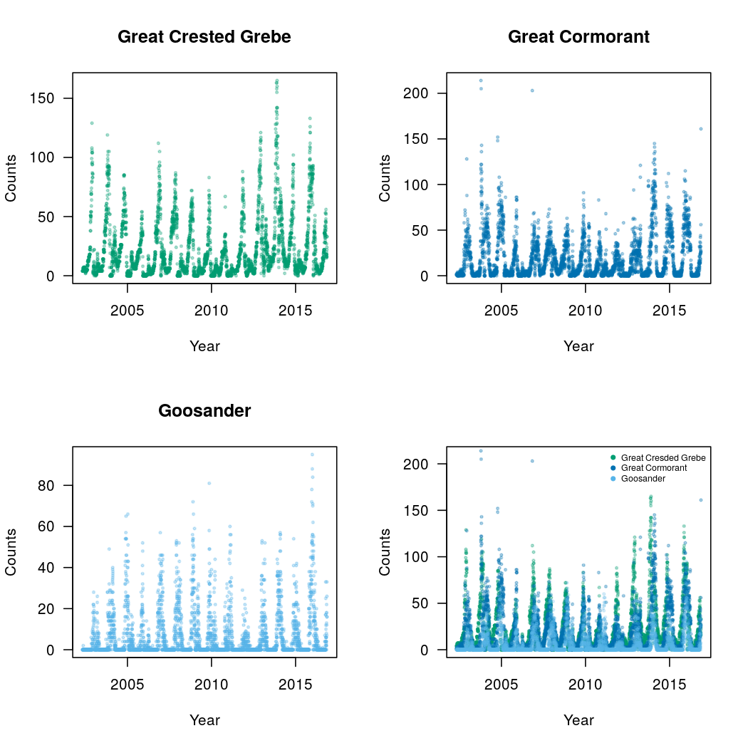
Figure 1: Time series for the three bird species Great Crested Grebe, Great Cormorant and Goosander at lake Seehammer See between May 2002 and November 2016.

In the study area, the abundances of all three species in winter increased during the second half of the 20th century such that carrying capacity was reached in the 1990s (Suter, 1995). A possible explanation for the logistic growth of the winter populations is that the food resources for these piscivores were limited. All three species forage fish of almost the same size (10–20 cm) by diving to a depth of 5 m. Thus, the three species show considerable overlap in their feeding niches. Accordingly, if resources are limiting, interspecific competition would be expected. In the absence of experimental intervention data, our aim was to detect interspecific competition via negative correlations in observed multivariate abundances (for details see Kinshofer et al. (2018)).

The analysis is based on daily counts of the three piscivorous bird species sampled at lake Seehammer See, which is located in the foothills of the Alps in southern Bavaria, about 40 km southeast of Munich. It has an area of 1.47 km², with an average depth of 3.8 m (maximum 12 m). Thus, the entire water body is accessible to the three bird species. A local ornithologist, Gerhard Kinshofer, counted the three species between May 1, 2002 and November 13, 2016 from various locations around the lake by using a spotting scope. He was therefore able to spot most, if not all, birds on the lake. As the sampling design was identical across all years, it can be safely assumed that any sampling error was the same over time. A total of 5,311 counts were available, with a few missing values either because data were not collected on that day due to adverse meteorological conditions or because one of the bird species was not spotted but the ornithologist was unsure whether it was definitely absent. Since our model required observations of all three bird species on the same day, about 6.7% of the instances in which values were missing were excluded such that finally 4,955 observation-days were included in our analyses.

2.2 Single-species models

As single-species distribution models we consider count transformation models as introduced by Siegfried and Hothorn (2020). They are the main building block of the novel species community distribution models constructed for the multivariate abundance data developed in Section 2.3. Univariate transformation models describing the impact of explanatory environmental variables $x$ on the distribution of the abundance of a single species described by the univariate count response $Y\in\{0,1,2,\dots\}$ rely on an unknown transformation of the response, which must be estimated from the data. On a technical level, these models consist of a fully parameterized, smooth, monotone non-decreasing transformation $\alpha:\mathbb{R}^{+}\rightarrow\mathbb{R}$ of the discrete response and of a function of the environmental variables $\eta(\text{\boldmath$x$})$ (for instance, one can consider a linear predictor $\eta(\text{\boldmath$x$})=\text{\boldmath$x$}^{\top}\text{\boldmath$\beta$}$). The discrete conditional distribution function (CDF) $F_{Y\mid\text{\boldmath$X$}=\text{\boldmath$x$}}$ is modeled directly through

$$F_{Y\mid\text{\boldmath$X$}=\text{\boldmath$x$}}(y\mid\text{\boldmath$x$})=\mathbb{P}_{Y\mid\text{\boldmath$X$}=\text{\boldmath$x$}}(Y\leq y\mid\text{\boldmath$x$})=F({\alpha}(\lfloor y\rfloor)-\eta(\text{\boldmath$x$}))$$ (1)

where $y\in\mathbb{R}^{+}$ is an arbitrary cut-off evaluated at the largest integer $\lfloor y\rfloor$ at most as large as $y$ and $F$ is an inverse link function. The choice of the $F$ will determine the interpretation of the function $\eta(\text{\boldmath$x$})$ in the model. For example, when $F=\Phi$ , then $\mathbb{E}(\alpha(Y)\mid\text{\boldmath$x$})=\eta(\text{\boldmath$x$})$ expresses the conditional mean of the transformed counts. An alternative and attractive method to interpret the model utilizes a connection to probabilistic index models. For a reference habitat $\text{\boldmath$x$}_{\text{Ref}}$, the area under the curve (AUC) or probabilistic index $\mathbb{P}(Y\preceq Y_{\text{Ref}}\mid\text{\boldmath$x$},\text{\boldmath$x$}_{\text{Ref}})$ describes the probability of observing fewer individuals in habitat $x$ than in the reference habitat. Under model (1) and $F=\Phi$, this probability is simply $\Phi((\eta(\text{\boldmath$x$})-\eta(\text{\boldmath$x$}_{\text{Ref}}))/\sqrt{2})$ (Thas et al., 2012). For other choices of $F$, parameter interpretations are listed in Table 1 in Siegfried and Hothorn (2020). The negative sign of $\eta(\text{\boldmath$x$})$ ensures that larger values of $\eta(\text{\boldmath$x$})$ correspond non-linearly to larger values of the conditional mean $\mathbb{E}(Y\mid\text{\boldmath$x$})$.

The conditional discrete density for an observed number of individuals $y\in\mathbb{N}$ is $f_{Y\mid\text{\boldmath$X$}=\text{\boldmath$x$}}(y\mid\text{\boldmath$x$})=\mathbb{P}_{Y\mid\text{\boldmath$X$}=\text{\boldmath$x$}}(Y=y\mid\text{\boldmath$x$})=\mathbb{P}_{Y\mid\text{\boldmath$X$}=\text{\boldmath$x$}}(Y\leq y\mid\text{\boldmath$x$})-\mathbb{P}_{Y\mid\text{\boldmath$X$}=\text{\boldmath$x$}}(Y\leq y-1\mid\text{\boldmath$x$})$, which we can rewrite as

$$f_{Y\mid\text{\boldmath$X$}=\text{\boldmath$x$}}(y\mid\text{\boldmath$x$})=F(\alpha(\lfloor y\rfloor)-\eta(\text{\boldmath$x$}))-F(\alpha(\lfloor y-1\rfloor)-\eta(\text{\boldmath$x$}))$$ (2)

where $\mathbb{P}(Y=y\mid\text{\boldmath$x$})\equiv 0$ for $y\notin\mathbb{N}$. The corresponding likelihood is equivalent to the interval-censored likelihood, in which an observed count $y$ is represented by the interval $(\underline{y},\overline{y}]=(y-1,y]$ for $y>0$. Siegfried and Hothorn (2020) estimated suitably parameterized functions $\alpha$ and $\eta$ by maximizing this likelihood.

2.3 Multi-species models

In the following, we develop a joint multivariate regression model for multivariate count data, that is, a model describing the joint distribution of several count variables conditional on a set of environmental explanatory variables. In the context of the aquatic bird competition problem (Section 2.1), the abundances of three species $\text{\boldmath$Y$}=(Y_{\text{A}},Y_{\text{B}},Y_{\text{C}})^{\top}\in\{0,1,2,\dots\}^{3}$ (A = Great Crested Grebe, B = Great Cormorant, C = Goosander) are modeled jointly, conditional on the time of year. To ensure the interpretability of the models, our presentation is limited to joint models allowing the marginal distribution of each species to be understood in terms of a univariate count transformation model (Section 2.2):

$$F_{Y_{j}\mid\text{\boldmath$X$}=\text{\boldmath$x$}}(y_{j}\mid\text{\boldmath$x$})=\mathbb{P}_{Y_{j}\mid\text{\boldmath$X$}=\text{\boldmath$x$}}(Y_{j}\leq y_{j}\mid\text{\boldmath$x$})=F(\alpha_{j}(\lfloor y_{j}\rfloor)-\eta_{j}(\text{\boldmath$x$}))$$ (3)

with counts $y_{j}\in\mathbb{N}$ for the three species $j=\text{A},\text{B},\text{C}$. We choose $F=\Phi$, alternative choices are discussed in Section 4. Furthermore, pairwise associations between species are made quantifiable on the scale of the transformed counts via a correlation coefficient. Multivariate conditional transformation models (Klein et al., 2020) for a continuous response vector $\text{\boldmath$Y$}=(Y_{1},Y_{2},Y_{3},\dots,Y_{J})^{\top}\in\mathbb{R}^{J}$ feature these types of simple expressions for the marginal and joint distributions; however, neither those models nor the inference procedures are directly applicable to count data. To extend the models to count data and for the sake of simplicity, we restrict the notation to $J=3$; the methodology applies to arbitrary dimensions $J\geq 2$.

In the univariate transformation model for a continuous response, it is assumed that a transformed version of the response follows a known distribution, such as a standard normal distribution in models with $F=\Phi$. Similarly, for a multivariate continuous response, we assume that the transformed data $\text{\boldmath$h$}(\text{\boldmath$Y$})=(h_{1}(\text{\boldmath$Y$}),h_{2}(\text{\boldmath$Y$}),h_{3}(\text{\boldmath$Y$}))^{\top}$ follow a multivariate normal distribution with mean zero. The correlation structure is defined by imposing a triangular structure on each of the component-wise transformation functions $h_{1}(\text{\boldmath$Y$}),h_{2}(\text{\boldmath$Y$}),h_{3}(\text{\boldmath$Y$})$ by formulating them as

$$h_{1}(\text{\boldmath$Y$})=h_{1}(Y_{1}),h_{2}(\text{\boldmath$Y$})=h_{2}(Y_{1},Y_{2}),\text{ and }h_{3}(\text{\boldmath$Y$})=h_{3}(Y_{1},Y_{2},Y_{3}).$$ (4)

Rationals explaining this choice are given in Klein et al. (2020). Each of these transformation functions is decomposed as a linear combination of marginal, monotone, non-decreasing transformation functions $\tilde{h}_{j}:\mathbb{R}\rightarrow\mathbb{R}$ with unknown parameters $\lambda_{21}$, $\lambda_{31}$, and $\lambda_{32}$. With $h_{1}(\text{\boldmath$Y$})=\tilde{h}_{1}(Y_{1})$, we can define $h_{2}(\text{\boldmath$Y$})=\lambda_{21}\tilde{h}_{1}(Y_{1})+\tilde{h}_{2}(Y_{2})$ and $h_{3}(\text{\boldmath$Y$})=\lambda_{31}\tilde{h}_{1}(Y_{1})+\lambda_{32}\tilde{h}_{2}(Y_{2})+\tilde{h}_{3}(Y_{3})$, or in more compact vector-matrix form,

$$\text{\boldmath$h$}(\text{\boldmath$y$})=\begin{pmatrix}[l]h_{1}(\text{\boldmath$y$})\\ h_{2}(\text{\boldmath$y$})\\ h_{3}(\text{\boldmath$y$})\end{pmatrix}=\begin{pmatrix}[l]h_{1}(y_{1})\\ h_{2}(y_{1},y_{2})\\ h_{3}(y_{1},y_{2},y_{3})\end{pmatrix}=\begin{pmatrix}[l]1&0&0\\ \lambda_{21}&1&0\\ \lambda_{31}&\lambda_{32}&1\end{pmatrix}\begin{pmatrix}[l]\tilde{h}_{1}(y_{1})\\ \tilde{h}_{2}(y_{2})\\ \tilde{h}_{3}(y_{3})\end{pmatrix}=\mathbf{\Lambda}\tilde{\text{\boldmath$h$}}(\text{\boldmath$y$})$$ (5)

for a lower triangular matrix $\mathbf{\Lambda}\in\mathbb{R}^{3\times 3}$ defined by the $\lambda$-parameters. The coefficients in $\mathbf{\Lambda}$ characterize the dependence structure of the transformed responses via a Gaussian copula, in which the joint (unconditional) distribution of $Y$ is given by

$$\mathbb{P}(\text{\boldmath$Y$}\leq\text{\boldmath$y$})=\Phi_{\mathbf{0},\mathbf{\Sigma}}\left[\Phi^{-1}_{0,\sigma_{11}^{2}}\{\Phi(y_{1})\},\Phi^{-1}_{0,\sigma_{22}^{2}}\{\Phi(y_{2})\},\Phi^{-1}_{0,\sigma_{33}^{2}}\{\Phi(y_{3})\}\right]$$

with variance-covariance matrix $\mathbf{\Sigma}=\mathbf{\Lambda}^{-1}\mathbf{\Lambda}^{-\top}$. This allows $\mathbf{\Lambda}$ to be interpreted as the inverse Cholesky factor of the variance-covariance matrix of the Gaussian copula. The $\lambda$-parameters thus describe the correlation of the transformed data $\text{\boldmath$h$}(\text{\boldmath$Y$})$. Correlation coefficients, the off-diagonal elements of $\text{diag}(\mathbf{\Sigma})^{-1/2}\,\mathbf{\Sigma}\,\text{diag}(\mathbf{\Sigma})^{-1/2}$, can be computed from $\mathbf{\Lambda}$. Information about the interaction of species can be described by Spearman’s rank correlations $\rho^{(S)}$: because the transformations $\text{\boldmath$h$}(\text{\boldmath$Y$})$ are monotone increasing, the rank correlations between species counts $Y$ can be computed from the correlations of $\text{\boldmath$h$}(\text{\boldmath$Y$})$, i.e., from the off-diagonal elements $\rho_{\tilde{k}k}$ of $\text{diag}(\mathbf{\Sigma})^{-1/2}\,\mathbf{\Sigma}\,\text{diag}(\mathbf{\Sigma})^{-1/2}$. The rank correlation of $(Y_{\tilde{k}},Y_{k})$ is given by $\rho^{(S)}(Y_{\tilde{k}},Y_{k})=\frac{6}{\pi}\text{arcsin}\left(\frac{\rho_{\tilde{k}k}}{2}\right)$.

Moreover, the Gaussian copula framework allows a formulation of the marginal distributions in terms of the transformation functions $\tilde{h}_{j}$ for $j=1,2,3$: $\Phi_{Y_{j}\mid\text{\boldmath$X$}=\text{\boldmath$x$}}(y_{j}\mid\text{\boldmath$x$})=\mathbb{P}(Y_{j}\leq y_{j}\mid\text{\boldmath$x$})=\Phi(\lfloor\tilde{h}_{j}(y_{j})\rfloor-\eta_{j}(\text{\boldmath$x$}))$ that is, $\tilde{h}_{j}$ is the transformation function of the marginal models and it is conditional only on environmental variables $x$. These marginal distribution models correspond to single-species distribution models.

In principle, not only the shift terms $\eta_{j}(\text{\boldmath$x$})$ but also the entries of $\mathbf{\Lambda}$ can depend on $x$, such that interactions between species may change with changes in habitat, space, or time. This dependence can be formulated entry-wise as:

$$\lambda_{\tilde{k}k}(\text{\boldmath$x$})=\text{\boldmath$x$}^{\top}\text{\boldmath$\tau$}_{\tilde{k}k}=\begin{cases}\tau_{\tilde{k}k}&\text{``Model }\text{M-}\mathbf{\Lambda}\text{''}\\ \tau_{\tilde{k}k}+\zeta_{\tilde{k}k}(\text{\boldmath$x$})&\text{``Model }\text{M-}\mathbf{\Lambda}(\text{\boldmath$x$})\text{''}\end{cases}\quad\text{for }1\leq k<\tilde{k}\leq J,$$ (6)

where $\tau_{\tilde{k}k}\in\mathbb{R}$ and $\zeta_{\tilde{k}k}(\text{\boldmath$x$})$ is a function of the environmental variables $x$. In the Gaussian copula framework, the coefficients $\lambda_{\tilde{k}k}(\text{\boldmath$x$})$ allow statements to be made about the independence of the components of the response vector. In model $\text{M-}\mathbf{\Lambda}$ it is assumed that the Spearman’s rank correlations between components of the random vector $Y$ is constant and model $\text{M-}\mathbf{\Lambda}(\text{\boldmath$x$})$ allows the Spearman’s rank correlation between species to vary depending on the environmental variables $x$, space, or time.

2.3.1 Likelihood inference

The log-likelihood for continuous observations $\text{\boldmath$y$}_{i}\in\mathbb{R}^{3},i=1,\dots,N$ under this continuous multivariate transformation model is given by

$$\ell(\text{\boldmath$\theta$})=\sum_{i=1}^{N}\log\left(\sum_{j=1}^{3}-\frac{1}{2}\left(\tilde{h}_{j}(y_{ij})+\sum_{\jmath=1}^{j-1}\lambda_{j\jmath}\tilde{h}_{\jmath}(y_{i\jmath})\right)^{2}\right)+\log\left(\tilde{h}_{j}^{\prime}(y_{ij})\right)$$ (7)

where $\text{\boldmath$\theta$}=(\text{\boldmath$\tilde{h}$},\mathbf{\Lambda})^{\top}$ contains the parameters of the model (see Section 2.4 for details). Hence, the parameters of the joint distribution of a continuous response vector can be readily estimated via maximum likelihood (see Appendix A). Introducing environmental variables $x$ into this unconditional model is straightforward: for conditional marginal distributions, the change $\tilde{h}_{j}(y_{ij})\rightarrow\tilde{h}_{j}(y_{ij})-\eta_{j}(\text{\boldmath$x$}_{i})$ is required and conditional correlations can be estimated by switching from model $\text{M-}\mathbf{\Lambda}$ to model $\text{M-}\mathbf{\Lambda}(\text{\boldmath$x$})$ in Equation 6.

Count data $\text{\boldmath$y$}_{i}\in\mathbb{N}^{3}$ can be viewed as interval-censored information. Instead of observing an exact continuous observation $\text{\boldmath$y$}_{i}\in\mathbb{R}^{3}$, the interval $(\underline{\text{\boldmath$y$}}_{i},\overline{\text{\boldmath$y$}}_{i}]=(\text{\boldmath$y$}_{i}-1,\text{\boldmath$y$}_{i}]$ is observed. Thus, for a count response vector $\text{\boldmath$Y$}=(Y_{\text{A}},Y_{\text{B}},Y_{\text{C}})^{\top}$ the exact log-likelihood of $\text{\boldmath$y$}_{i},i=1,\dots,N$ in this framework is given by

$$\ell(\text{\boldmath$\theta$})=\sum_{i=1}^{N}\log\left(\int_{\tilde{\text{\boldmath$h$}}(\underline{\text{\boldmath$y$}}_{i})}^{\tilde{\text{\boldmath$h$}}(\overline{\text{\boldmath$y$}}_{i})}\phi_{\mathbf{0},\mathbf{\Sigma}}(\tilde{\text{\boldmath$z$}})d\tilde{\text{\boldmath$z$}}\right)$$ (8)

where $\tilde{\text{\boldmath$h$}}(\underline{\text{\boldmath$y$}})=\left(\tilde{h}_{\text{A}}(\underline{y}_{\text{A}}),\tilde{h}_{\text{B}}(\underline{y}_{\text{B}}),\tilde{h}_{\text{C}}(\underline{y}_{\text{C}})\right)^{\top}$, $\tilde{\text{\boldmath$h$}}(\overline{\text{\boldmath$y$}})=\left(\tilde{h}_{\text{A}}(\overline{y}_{\text{A}}),\tilde{h}_{\text{B}}(\overline{y}_{\text{B}}),\tilde{h}_{\text{C}}(\overline{y}_{\text{C}})\right)^{\top}$, and $\phi_{\mathbf{0},\mathbf{\Sigma}}$ is the density of the trivariate normal with mean zero and covariance $\mathbf{\Sigma}$. Maximum-likelihood estimation of the parameters $\theta$ in Equation 8 is computationally extremely challenging, because higher-dimensional normal integrals have to be evaluated. Moreover, it is not possible to derive analytic expressions for the scores of the parameters. For this reason, in Sections 2.3.2 and 2.3.3 we introduce two computationally attractive approximations of the exact log-likelihood $\ell(\text{\boldmath$\theta$})$ to estimate the multi-species count transformation model.

2.3.2 Continuous approximation

In the first approximation, all counts are transformed as follows

$$\tilde{y}=\begin{cases}y-0.5&y\geq 1\\ y&y=0.\end{cases}$$ (9)

That is, this transformation is applied component-wise to a count vector $\text{\boldmath$y$}=(y_{\text{A}},y_{\text{B}},y_{\text{C}})^{\top}$ and the mid-points of the intervals $(y_{\text{A}}-1,y_{\text{A}}]$, $(y_{\text{B}}-1,y_{\text{B}}]$, and $(y_{\text{C}}-1,y_{\text{C}}]$ respectively are obtained. Then, because the resulting random vector is no longer a count vector, a multivariate conditional transformation model is fit maximizing (7) as described in Klein et al. (2020). In the univariate context, this approximation corresponds to the principle of applying least-squares to $\log(y+1)$ for parameter estimation and inference (e.g.,  Ives, 2015; Dean et al., 2017; Gotelli and Ellison, 2013; De Felipe et al., 2019; Mooney et al., 2016).

The log-likelihood contribution $\ell(\text{\boldmath$\theta$})=\log(f_{\text{\boldmath$Y$}}(\tilde{\text{\boldmath$y$}}\mid\text{\boldmath$\theta$}))$ for a transformed datum $\tilde{\text{\boldmath$y$}}$ is then (with $\phi=\Phi^{\prime}$):

$$\ell(\text{\boldmath$\theta$}) = \log\left(\phi\left(\tilde{h}_{\text{A}}(\tilde{y}_{\text{A}})\right)\right)+\log\left(\frac{\partial\tilde{h}_{\text{A}}(\tilde{y}_{\text{A}})}{\partial\tilde{y}_{\text{A}}}\right)+$$

$$\quad\log\left(\phi\left(\tilde{h}_{\text{B}}(\tilde{y}_{\text{B}})+\lambda_{\text{A}\text{B}}\tilde{h}_{\text{A}}(\tilde{y}_{\text{A}})\right)\right)+\log\left(\frac{\partial\tilde{h}_{\text{B}}(\tilde{y}_{\text{B}})}{\partial\tilde{y}_{\text{B}}}\right)+$$

$$\quad\log\left(\phi\left(\tilde{h}_{\text{C}}(\tilde{y}_{\text{C}})+\lambda_{\text{A}\text{C}}\tilde{h}_{\text{A}}(\tilde{y}_{\text{A}})+\lambda_{\text{B}\text{C}}\tilde{h}_{\text{B}}(\tilde{y}_{\text{B}})\right)\right)+\log\left(\frac{\partial\tilde{h}_{\text{C}}(\tilde{y}_{\text{C}})}{\partial\tilde{y}_{\text{C}}}\right).$$

Suitably parameterized choices of $\tilde{h}_{j}$ and $\mathbf{\Lambda}$ can then be estimated by maximum-likelihood; details are discussed in Appendix A.

2.3.3 Discrete approximation

It is also possible to approximate the integral of Equation 8 directly as follows. Note that if $\text{\boldmath$Z$}\sim\operatorname{N}(\mathbf{0},\mathbf{\Sigma})$ then $\mathbf{\Lambda}\text{\boldmath$Z$}\sim\operatorname{N}(\mathbf{0},\mathbf{\Lambda}\mathbf{\Sigma}\mathbf{\Lambda}^{\top}=\text{\boldmath$I$})$ with $\text{det}(\mathbf{\Lambda})=1$. A change of variables leads to

$$\exp(\ell(\text{\boldmath$\theta$})) = \int_{\mathbf{\Lambda}\tilde{\text{\boldmath$h$}}(\underline{\text{\boldmath$y$}})}^{\mathbf{\Lambda}\tilde{\text{\boldmath$h$}}(\overline{\text{\boldmath$y$}})}\phi_{\mathbf{0},\text{\boldmath$I$}}(\text{\boldmath$z$})\,d\text{\boldmath$z$}$$

$$\approx \left[\Phi(\tilde{h}_{\text{A}}(\overline{y}_{\text{A}}))-\Phi(\tilde{h}_{\text{A}}(\underline{y}_{\text{A}}))\right]\times$$

$$\quad\,\left[\Phi(\tilde{h}_{\text{B}}(\overline{y}_{\text{B}})+\lambda_{\text{A}\text{B}}\tilde{h}_{\text{A}}(\tilde{y}_{\text{A}}))-\Phi(\tilde{h}_{\text{B}}(\underline{y}_{\text{B}})+\lambda_{\text{A}\text{B}}\tilde{h}_{\text{A}}(\tilde{y}_{\text{A}}))\right]\times$$

$$\quad\,\Big{[}\Phi(\tilde{h}_{\text{C}}(\overline{y}_{\text{C}})+\lambda_{\text{A}\text{B}}\tilde{h}_{\text{A}}(\tilde{y}_{\text{A}})+\lambda_{\text{B}\text{C}}\tilde{h}_{\text{B}}(\tilde{y}_{\text{B}}))-$$

$$\qquad\quad\Phi(\tilde{h}_{\text{C}}(\underline{y}_{\text{C}})+\lambda_{\text{A}\text{B}}\tilde{h}_{\text{A}}(\tilde{y}_{\text{A}})+\lambda_{\text{B}\text{C}}\tilde{h}_{\text{B}}(\tilde{y}_{\text{B}}))\Big{]}$$

where $h_{\text{A}}(\text{\boldmath$y$}),h_{\text{B}}(\text{\boldmath$y$}),h_{\text{C}}(\text{\boldmath$y$})$ are defined as $h_{1},h_{2},h_{3}$ in Equation 5. This approximation relies on a simplifying assumption concerning the integration limits of the multivariate integral. Technical details are provided in Appendix A. This approximation to the likelihood resembles the correspondence between the exact discrete univariate likelihood (2) and the interval-censored case.

The quality of the two approximations to the exact likelihood (Equation 8) for the aquatic bird competition problem is evaluated by a parametric bootstrap procedure (Appendix A.5).

2.4 Parametrization and inference

In this section we discuss the technical aspects of the parameterization of the transformation functions $\tilde{h}_{j}=\alpha_{j}$, the shift functions $\eta_{j}$, and the inverse Cholesky factor $\mathbf{\Lambda}$, as well as details of the implementation and computation of these models.

The univariate transformation functions $\alpha_{j}:\mathbb{R}^{+}\rightarrow\mathbb{R}$, $j=$ A, B, C, are continuous and monotonically non-decreasing. They are applied to the largest integer $\lfloor y\rfloor$ at most as large as $y$ for an arbitrary cut-off point $y\in\mathbb{R}^{+}$ (Siegfried and Hothorn, 2020). Following the approach of Hothorn et al. (2018), the functions $\alpha_{j}(y)=\text{\boldmath$a$}_{j}(y)^{\top}\text{\boldmath$\vartheta$}_{j}$ are parameterized in terms of basis functions $\text{\boldmath$a$}_{j}:\mathbb{R}\rightarrow\mathbb{R}^{P}$ and are evaluated only at integer arguments $y\in\mathbb{N}$. For the models presented in Section 3, the $P$-dimensional Bernstein basis leading to polynomials in Bernstein form of order $P-1$ were used. This choice is computationally attractive and monotonicity can be achieved by imposing the constraint $\vartheta_{j,1}\leq\dots\leq\vartheta_{j,P}$ on the parameters $\text{\boldmath$\vartheta$}_{j}=(\vartheta_{j,1},\dots,\vartheta_{j,P})^{\top}\in\mathbb{R}^{P}$ for species $j$.

In general, the flexibility of a transformation function $\alpha_{j}$ can be adjusted in different ways: first, by choosing the degree of the Bernstein basis appropriately (Hothorn, 2020), and second by allowing the transformation function to depend on both the counts $y_{j}$ and the environmental variables $x$ with a more sophisticated model of the form $\alpha_{j}(y_{j}\mid\text{\boldmath$x$})=\text{\boldmath$a$}_{j}(y_{j})^{\top}\text{\boldmath$\vartheta$}_{j}(\text{\boldmath$x$})$.

For model $\text{M-}\mathbf{\Lambda}$, the lower $J\times(J-1)/2$ triangular elements of the inverse Cholesky factor $\mathbf{\Lambda}$ are constants. In the more complex setup of model $\text{M-}\mathbf{\Lambda}(\text{\boldmath$x$})$, each of these lower triangular elements is formulated as $\lambda_{\tilde{k}k}(\text{\boldmath$x$})=\tau_{\tilde{k}k}+\text{\boldmath$x$}^{\top}\zeta_{\tilde{k}k}$. As a consequence, Spearman’s rank correlations between the three species are allowed to vary with the day of the year.

The model formulation and the two approximations of the exact log-likelihood enable the estimation of all parameters jointly by maximum likelihood. Analytical expressions for the score functions are available for both approximations (see Appendix A) and thus standard optimizers can be employed for fast model inference. The variance-covariance matrix of all model parameters can be obtained from the numerically evaluated Hessian; corresponding Wald confidence intervals for selected model parameters are available (Klein et al., 2020).

2.5 Models for the aquatic birds: in search of competitive interactions

We developed a single model aimed at answering two questions derived from the hypothesis that the bird species compete for a common and limited resource: (1) How does the abundance of each species vary over the course of a year? (2) What is the pairwise correlation among the three species, i.e., is there a higher likelihood of observing large counts of individuals in pairs of considered species? Are the species counts independent or is a high abundance of the one species accompanied by a small abundance of the other?

We formulated two nested models sharing the same marginal structure

$$F_{Y_{j}\mid\text{\boldmath$X$}=\text{\boldmath$x$}}(y_{j}\mid\text{\boldmath$x$})=\Phi(\alpha_{j}(\lfloor y_{j}\rfloor)-\eta_{j}(\text{Year, Day})),\quad j=\text{A},\text{B},\text{C}$$ (11)

describing the abundance of each species for each day (1 to 365) within each year of the observation period (2002 to 2016). Two nested choices for the dependence structure (6) were applied: a multivariate model $\text{M-}\mathbf{\Lambda}$ assuming time-constant Spearman’s rank correlations between all three species, and a multivariate model $\text{M-}\mathbf{\Lambda}(\text{\boldmath$x$})$ that allows the pairwise Spearman’s correlations to change over the course of a year. The correlations are modeled as a smooth annual function by parametrizing $\mathbf{\Lambda}(\text{\boldmath$x$})$ appropriately, details can be found in the Appendix A. It is important to note that, because all model parameters were estimated simultaneously, the marginal models of $\text{M-}\mathbf{\Lambda}$ and $\text{M-}\mathbf{\Lambda}(\text{\boldmath$x$})$ implicitly account for correlations among the three bird species.

Among all models from the literature on species distribution modeling, we benchmarked our model against the best performing model according to the review by Norberg et al. (2019): the joint species distribution model Hierarchical Modeling of Species Communities (Hmsc) (Ovaskainen et al., 2017). Hmsc was developed to analyze multivariate data from species communities. After specifying the marginal models (in our case, marginal Poisson models with log link), the Hmsc model is fitted with Bayesian inference through MCMC sampling. Hmsc allows the estimation of so-called species-to-species associations by a latent factor approach, that is, including a random effect on the sampling unit level. Moreover, it is possible to incorporate covariate, temporal or spatial dependencies in the random effect, making Hmsc conceptually similar to model $\text{M-}\mathbf{\Lambda}(\text{\boldmath$x$})$.

3 Results

The latent correlations and Spearmans’s rank correlations estimated from model $\text{M-}\mathbf{\Lambda}$ are given in Table 1, together with the 95% confidence intervals. The correlations and confidence intervals between Great Cormorant and Great Crested Grebe were very similar in a comparison of the continuous and discrete approximations. Correlations involving Goosander, due to the smaller number of counts, led to larger discrepancies for this species.

The estimated time-dependent Spearman’s rank correlations from model $\text{M-}\mathbf{\Lambda}(\text{\boldmath$x$})$ are presented in Figures 3 and 9 for the discrete and continuous approximations respectively. All three pairwise correlations were described by a U-shaped function, with higher correlations of around $0.5$ in December and January and correlations close to zero between June and October.

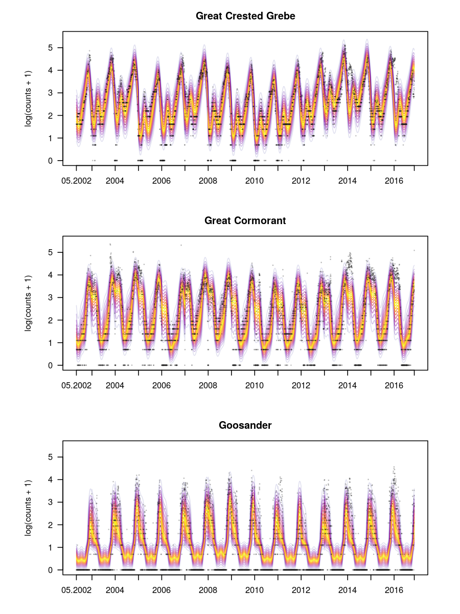
Figure 8: Model $\text{M-}\mathbf{\Lambda}(\text{\boldmath$x$})$, continuous approximation: univariate marginal distributions conditional on time for the three bird species.

The marginal distributions are given in Figures 2 and 7 for model $\text{M-}\mathbf{\Lambda}$, and in Figure 6 and Figure 8 for model $\text{M-}\mathbf{\Lambda}(\text{\boldmath$x$})$, for the discrete and the continuous approximations respectively. The annual pattern was the same as in the other models but discrepancies between the two approximations were larger.

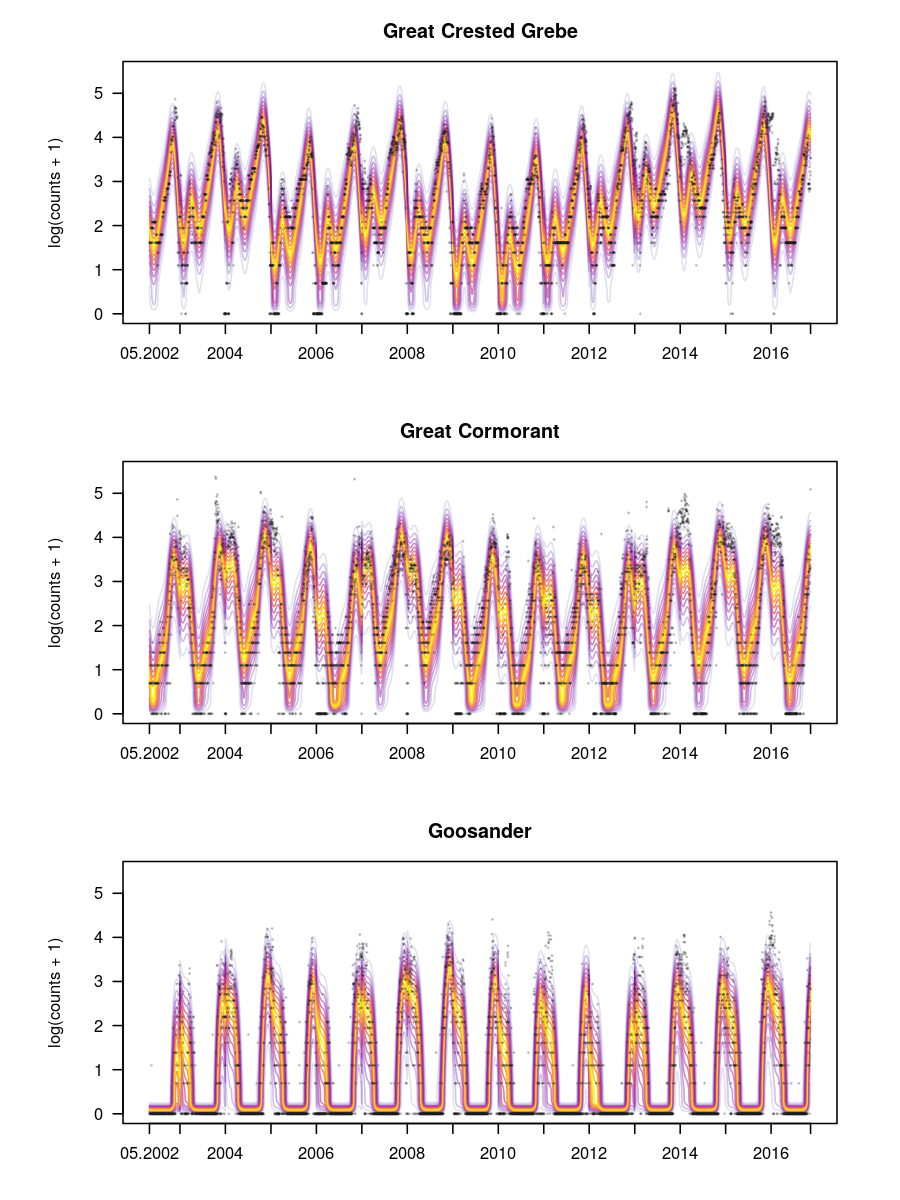
Figure 2: Model $\text{M-}\mathbf{\Lambda}$, discrete approximation: univariate marginal distributions conditional on time for the three bird species. The $x$-axis indicates the time frame when the data were collected. The $y$-axis indicates the natural logarithm of the counts, augmented by one.

Table 1: Measures of dependendence between three bird species from model $\text{M-}\mathbf{\Lambda}$
Continuous approximation Discrete approximation $\hat{\lambda}_{\text{A},\text{B}}$ $-0.483$ $[-0.514,-0.452]$ $-0.467$ $[-0.500,-0.435]$ $\hat{\lambda}_{\text{A},\text{C}}$ $-0.200$ $[-0.232,-0.168]$ $-0.202$ $[-0.241,-0.164]$ $\hat{\lambda}_{\text{B},\text{C}}$ $-0.219$ $[-0.247,-0.190]$ $-0.244$ $[-0.284,-0.204]$ $\hat{\rho}_{\text{A},\text{B}}$ $-$$0.435$ $[0.411,0.458]$ $-$$0.423$ $[0.398,0.448]$ $\hat{\rho}_{\text{A},\text{C}}$ $-$$0.286$ $[0.260,0.310]$ $-$$0.294$ $[0.263,0.324]$ $\hat{\rho}_{\text{B},\text{C}}$ $-$$0.309$ $[0.283,0.333]$ $-$$0.330$ $[0.295,0.362]$ $\hat{\rho}_{\text{A},\text{B}}^{(S)}$ $-$$0.419$ $[0.396,0.441]$ $-$$0.407$ $[0.383,0.431]$ $\hat{\rho}_{\text{A},\text{C}}^{(S)}$ $-$$0.274$ $[0.249,0.298]$ $-$$0.281$ $[0.252,0.311]$ $\hat{\rho}_{\text{B},\text{C}}^{(S)}$ $-$$0.296$ $[0.271,0.320]$ $-$$0.316$ $[0.282,0.348]$

Table 1: Model $\text{M-}\mathbf{\Lambda}$: the first three rows of the table show point estimates for the inverse Cholesky factor $\mathbf{\Lambda}$ and the 95% Wald confidence intervals. Rows 4 to 6 show the resulting constant correlations $\rho$ and the 95% confidence intervals based on the asymptotic distribution of the parameters of model $\text{M-}\mathbf{\Lambda}$. The last three rows show the corresponding Spearman’s rank correlation $\rho^{(S)}$ with 95% confidence intervals based on the asymptotic distribution of the parameters of model $\text{M-}\mathbf{\Lambda}$. A: Great Cormorant, B: Great Crested Grebe, C: Goosander.

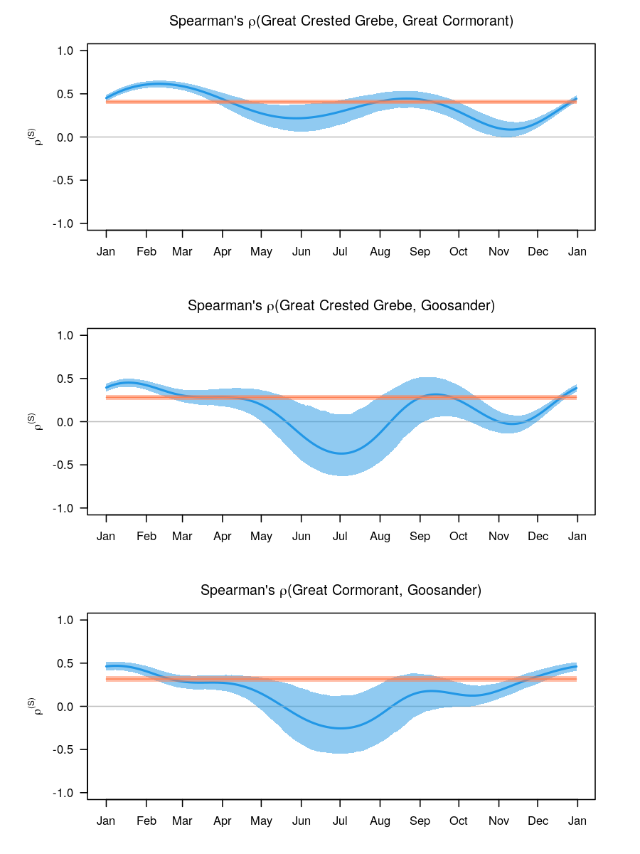
Figure 3: Model $\text{M-}\mathbf{\Lambda}(\text{\boldmath$x$})$, discrete approximation: trajectories of the pairwise Spearman’s rank correlations $\rho^{(S)}$ across species over one year and the corresponding 95% confidence intervals based on the asymptotic distribution of the parameters. For comparison, the constant Spearman’s rank correlations of model $\text{M-}\mathbf{\Lambda}$ (see Table 1) are plotted in orange with the corresponding 95% confidence intervals.

Because the two models $\text{M-}\mathbf{\Lambda}$ and $\text{M-}\mathbf{\Lambda}(\text{\boldmath$x$})$ are nested, they can be compared in a likelihood-ratio test. The result is the same for the two approximations, with strong evidence in favor of the more complex model $\text{M-}\mathbf{\Lambda}(\text{\boldmath$x$})$ over the simpler model $\text{M-}\mathbf{\Lambda}$. For the discrete approximation, the log-likelihoods are $-42357.4$ for $\text{M-}\mathbf{\Lambda}$ and $-42246$ for $\text{M-}\mathbf{\Lambda}(\text{\boldmath$x$})$. Because the more complex model $\text{M-}\mathbf{\Lambda}(\text{\boldmath$x$})$ has $18$ parameters more than model $\text{M-}\mathbf{\Lambda}$, we compare twice the difference of the log-likelihoods of $\text{M-}\mathbf{\Lambda}(\text{\boldmath$x$})$ and $\text{M-}\mathbf{\Lambda}$ with a one-sided chi-squared distribution with 18 degrees of freedom and obtain strong evidence ($p<0.0001$) in favor of the more complex model $\text{M-}\mathbf{\Lambda}(\text{\boldmath$x$})$.

The main motivation for multi-species count transformation models is to identify interspecies dependencies. We performed a parametric bootstrap comparison between multi-species count transformation models and Hmsc: one hundred new data sets were sampled from a model assuming time-constant correlations between the three aquatic bird species (model $\text{M-}\mathbf{\Lambda}$ fitted to the original data). For each of these 100 data sets, we compared Spearman’s rank correlations estimated by multi-species count transformation models and residual correlations obtained from Hmsc to the ground truth, i.e., the Spearman’s rank correlations from model $\text{M-}\mathbf{\Lambda}$ fitted to the original data (Figure 4). The same exercise was performed for model $\text{M-}\mathbf{\Lambda}(\text{\boldmath$x$})$.

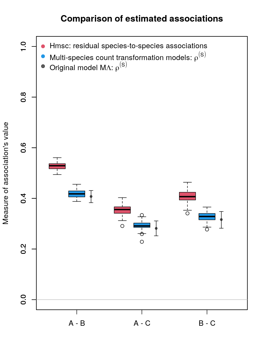
Figure 4: Measures of species-to-species associations for Hmsc (residual species-to-species association) and mcotram (Spearman’s rank correlation) obtained from refitting the models on 100 independent data sets simulated from model $\text{M-}\mathbf{\Lambda}$. A: Great Cormorant, B: Great Crested Grebe, C: Goosander.

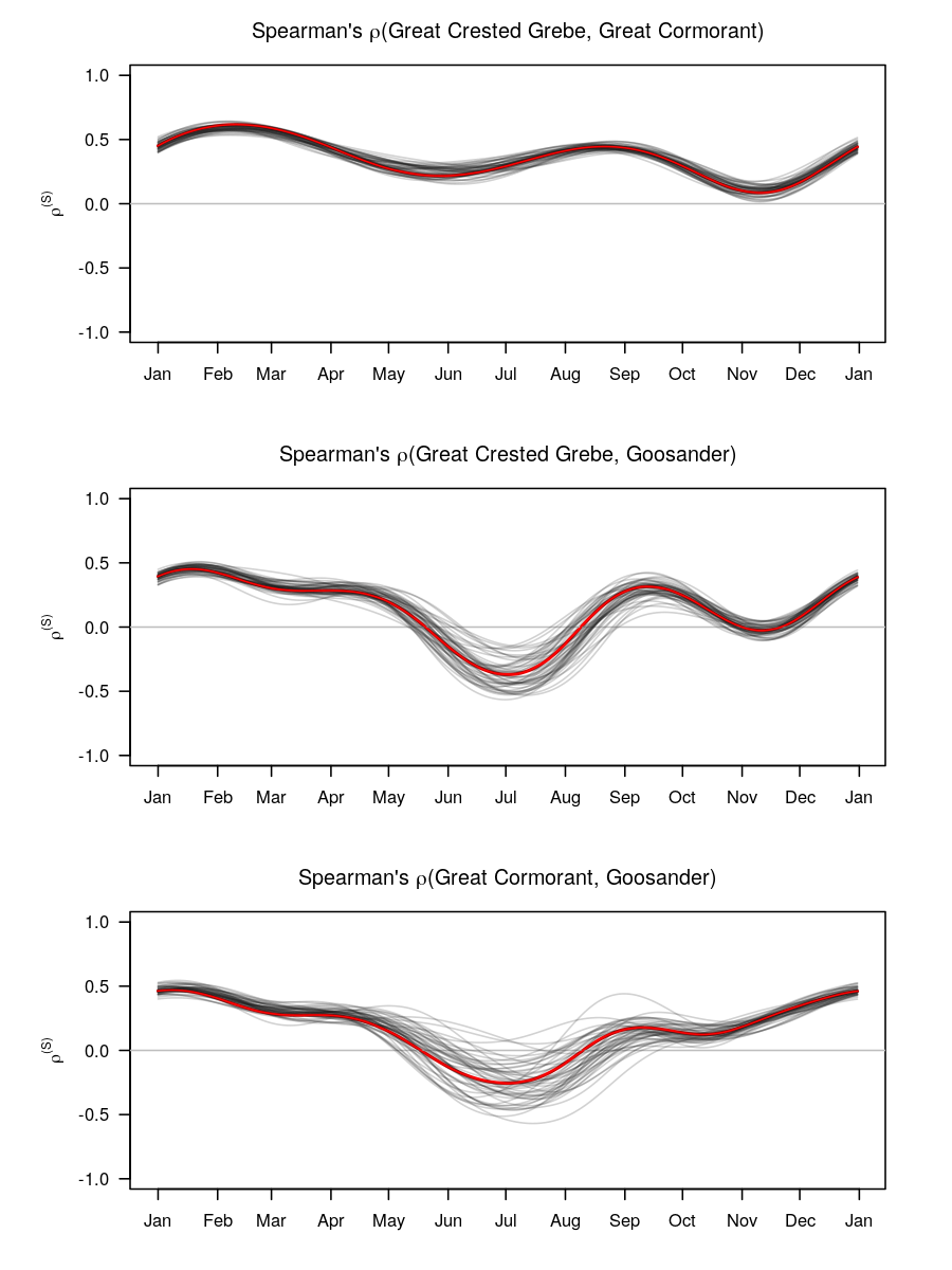
Figure 5: Yearly trajectories of Spearman’s rank correlations from the models fitted on the 100 bootstrapped data sets (grey lines) and from the original model $\text{M-}\mathbf{\Lambda}(\text{\boldmath$x$})$ (red line).

Multi-species count transformation models detected the true Spearman’s correlations from samples of the original model accurately and with precision. The uncertainty obtained from the parametric bootstrap was comparable to the uncertainty reported by the 95% confidence interval for Spearman’s correlation in the original model (Table 1). This also indicates correctness of likelihood-based inference as described in Section 2.4. Hmsc identified a similar correlation pattern with equally high precision, the model formulation underlying Hmsc however does not allow to derive Spearman’s correlations for counts and we could not expect the residual correlations being in line with the ground truth in this setting.

For time-varying dependencies, multi-species count transformation models picked up this signal from bootstrapped data sets, the uncertainty (Figure 5) matched the uncertainty reported by confidence intervals obtained from the original model (Figure 3). Conceptually, a similar analysis can be performed by Hmsc (Tikhonov et al., 2017), however did not succeed yet in extracting this information from models fitted with version 3.0-11 of package Hmsc.

Re-fitting multi-species count transformation models is in general much faster than re-fitting Hmsc models to the same data. The computation time for Hmsc depends on parameters for MCMC sampling, which we defined as in the package’s vignette. On average, fitting the multi-species transformation model $\text{M-}\mathbf{\Lambda}$ to 4955 observations took 15.3 seconds, the more complex model $\text{M-}\mathbf{\Lambda}(\text{\boldmath$x$})$ required 15.7 seconds. Fitting a poisson model fitting Hmsc took 424 seconds on average.

4 Discussion

Multi-species count transformation models provide a new perspective on joint models for species distributions, as they take both the habitat and community aspects into account. Although the technical details are challenging, we are confident that at least simple forms of the models will be of value in ecological modeling. In contrast to JSDMs, i.e., generalized mixed models in which the community aspect is represented by an unstructured random residual term, transformation models do not require strict distributional assumptions but they still offer interpretability of marginal and joint effects. Pairwise relationships between species can be understood as correlations on a latent normal scale, and marginal effects expressed as the means of transformed counts or as AUCs.

Conceptually, multi-species count transformation models differ from standard approaches in MSDM and JSDM in two ways. First, we do not make any assumptions about a parametric distribution of the counts, such as Poisson or negative binomial. Instead, the distribution is estimated in a data-driven way. Second, measures of dependence (Pearson’s correlation on a latent scale, or Spearman’s rank correlations on the original scale of the counts) are estimated simultaneously to all other model parameters and can be computed directly from identifiable quantities estimated in our model. Most MSDMs and JSDMs do not provide such quantities directly and if they do, they often resort to the fixed-/random effects dichotomy which inevitably influences the interpretation of the model parameters. Consequently, multi-species count transformation models allow to answer a broader class of research question that involve the dependency of the relation between different species to depend on covariates $x$. This interesting feature enabling habitat-dependent modeling of pairwise correlations on a latent scale accommodates spatio-temporal variations in species interactions in addition to possible spatio-temporal trends in marginal abundances. In the relatively simple models for aquatic bird competition presented herein, the marginal abundances of the three fish-eating bird species were shown to vary systematically over the course of a year (hypothesis 1, reflecting different habitat requirements particularly during the breeding period in summer), with moderate positive correlations determined in winter and early spring, and small and highly variable correlations during the rest of the year (hypothesis 2). Thus, the results of the final model indicate that competition is not a driving factor regulating the abundance of these bird species in the study area. Unlike the seasonal variation, which is clearly represented in the time-series plots of the observations, correlations cannot be inferred from the raw data in the absence of a suitable model.

Multi-species count transformation models are currently limited in three different ways. (1) We restricted our attention to latent Gaussian models with $F=\Phi$. From a marginal perspective, other choices might be more interesting, such as using the inverse logit link $F=\text{logit}^{-1}$, which allows the interpretation of the shift terms $\eta_{j}(\text{\boldmath$x$})$ as log-odds ratios. Model estimation is implemented in cotram for a range of alternatives. (2) with non-constant parameters $\mathbf{\Lambda}(\text{\boldmath$x$})$ in the inverse Cholesky factor, the model is not as lean on assumptions as a model with constant correlations, i.e., constant parameters in $\mathbf{\Lambda}$. Concretely, the parameter estimates resulting from the joint model might depend on the order in which the marginal models are specified. This effect can be counterbalanced by accounting for enough flexibility in the marginal models, as explained in a simple example provided in Appendix A. (3) Complex models can be specified for the marginal shift terms $\eta_{j}(\text{\boldmath$x$})$ and for components of the Cholesky factor $\mathbf{\Lambda}(\text{\boldmath$x$})$, for example by including either nonlinear or lagging effects of explanatory environmental variables or terms capturing spatio-temporal trends for correlated observations. However, in such cases the likelihood approximations proposed here require supplementation with appropriate smoothness constraints. A mixed version of univariate transformation models that is also applicable to count transformation models was recently proposed (Tamási and Hothorn, 2021; Tamási et al., 2022) and can handle spatially or otherwise correlated data. However, the technical challenges associated with mixed transformation models on the one hand and multi-species count transformation models on the other clearly demonstrate that significant improvements in this direction will require substantial research efforts. With respect to nonlinear habitat effects, a pragmatic approach might be to estimate univariate SDMs separately for each species, thus allowing a nonlinear impact of environmental variables. The joint models could then be fitted with the same functional form as that of the marginal shift terms $\eta_{j}(\text{\boldmath$x$})$.

Based on our empirical results as well as the theoretical and empirical results presented in Klein et al. (2020) and Siegfried and Hothorn (2020), the following can be recommended when using the model: (1) For count data with large or at least moderate numbers of counts and few zeros, application of the continuous approximation to multi-species count transformation models with constant $\mathbf{\Lambda}$ is possible for small and moderate numbers of species (Klein et al., 2020, report results for up to $J=10$). (2) For small counts and data with many zeros, the discrete approximation should be employed. (3) Models with habitat-dependent correlations $\mathbf{\Lambda}(\text{\boldmath$x$})$ should be estimated for different permutations of the species in a sensitivity analysis. Both the ordering of species with increasing variance and the introduction of habitat-dependencies into transformation functions as in model $\text{M-}\mathbf{\Lambda}(\text{\boldmath$x$})$ are recommended. In general, a strong dependency of the parameter estimates on the order of species indicates a severe lack of model fit.

The approaches discussed herein are quite complex and far-removed from those typically employed for species distribution modeling. Multivariate transformation models cannot be viewed as extensions of established models, such as generalized linear mixed models. Model interpretation requires an understanding of latent, transformed scales, especially on the marginal scale. Nevertheless, in our proof-of-concept application, we demonstrated that interesting insights into the interplay between species can be obtained from a simple version of the model. The implementation of a similar analysis using concepts from established MSDMs and JSDMs is likely to be technically much more difficult. In summary, the extension of single-species distribution models to models for species communities remains conceptually challenging. While not offering a one-size-fits-all solution, multivariate transformation models provide an alternative approach to the problem.

Computational details

All computations were performed using R version 4.1.2 (R Core Team, 2021). Multi-species count transformation models are implemented in the cotram add-on package (Siegfried et al., 2022). The package includes reproducibility material for the empirical results presented in Section 3 and the Appendix A. Models and figures can be replicated by

install.packages("cotram")
library("cotram")
demo("aquabirds", package = "cotram")

The continuous approximation (Section 2.3.2) relies on implementation of the multivariate conditional transformation models in package tram (Hothorn and Barbanti, 2022). The competitor model Hmsc was fitted with the package Hmsc (Tikhonov et al., 2021).

Appendix A Appendix

A.1 Continuous approximation

The log-likelihood and scores for the continuous approximation can be found in Klein et al. (2020) for the general case $J\geq 2$. For our application, these quantities were evaluated on the transformed version of the counts, $\tilde{\text{\boldmath$y$}}$ described in Equation 9.

A.2 Discrete approximation

For a simpler notation, the species A, B, C are converted to indexes $1,2$ and $3=J$ respectively. These expressions generalize directly to the case with $J$ species.

The approximation in Equation 2.3.3 is obtained as follow: because the integration limits are non-constant, the simplifying assumption is made that each integration limit varies only with respect to one coordinate, and (where this make sense) the two other coordinates are substituted with the transformed version of Equation 9. This allows the integral to be “split” into three parts that can be evaluated independently of each other:

$$\exp(\ell(\text{\boldmath$\theta$}))=\int_{\mathbf{\Lambda}\tilde{\text{\boldmath$h$}}(\underline{\text{\boldmath$y$}})}^{\mathbf{\Lambda}\tilde{\text{\boldmath$h$}}(\overline{\text{\boldmath$y$}})}\phi_{\mathbf{0},\text{\boldmath$I$}}(\text{\boldmath$z$})\,d\text{\boldmath$z$}$$

$$=\int_{h_{\text{A}}(\underline{\text{\boldmath$y$}})}^{h_{\text{A}}(\overline{\text{\boldmath$y$}})}\int_{h_{\text{B}}(\underline{\text{\boldmath$y$}})}^{h_{\text{B}}(\overline{\text{\boldmath$y$}})}\int_{h_{\text{C}}(\underline{\text{\boldmath$y$}})}^{h_{\text{C}}(\overline{\text{\boldmath$y$}})}\phi(z_{\text{A}})\phi(z_{\text{B}})\phi(z_{\text{C}})\,dz_{\text{C}}\,dz_{\text{B}}\,dz_{\text{A}}$$

$$\approx\int_{h_{\text{A}}(\underline{y}_{\text{A}})}^{h_{\text{A}}(\overline{y}_{\text{A}})}\int_{h_{\text{B}}((\tilde{y}_{\text{A}},\underline{y}_{\text{B}})^{\top})}^{h_{\text{B}}((\tilde{y}_{\text{A}},\overline{y}_{\text{B}})^{\top})}\int_{h_{\text{C}}((\tilde{y}_{\text{A}},\tilde{y}_{\text{B}},\underline{y}_{\text{C}})^{\top})}^{h_{\text{C}}((\tilde{y}_{\text{A}},\tilde{y}_{\text{B}},\overline{y}_{\text{C}})^{\top})}\phi(z_{\text{C}})\phi(z_{\text{B}})\phi(z_{\text{A}})\,dz_{\text{C}}\,dz_{\text{B}}\,dz_{\text{A}}$$

$$=\int_{h_{\text{A}}(\underline{y}_{\text{A}})}^{h_{\text{A}}(\overline{y}_{\text{A}})}\phi(z_{\text{A}})\,dz_{\text{A}}\int_{h_{\text{B}}((\tilde{y}_{\text{A}},\underline{y}_{\text{B}})^{\top})}^{h_{\text{B}}((\tilde{y}_{\text{A}},\overline{y}_{\text{B}})^{\top})}\phi(z_{\text{B}})\,dz_{\text{B}}\int_{h_{\text{C}}((\tilde{y}_{\text{A}},\tilde{y}_{\text{B}},\underline{y}_{\text{C}})^{\top})}^{h_{\text{C}}((\tilde{y}_{\text{A}},\tilde{y}_{\text{B}},\overline{y}_{\text{C}})^{\top})}\phi(z_{\text{C}})\,dz_{\text{C}}$$

$$=\left[\Phi(\tilde{h}_{\text{A}}(\overline{y}_{\text{A}}))-\Phi(\tilde{h}_{\text{A}}(\underline{y}_{\text{A}}))\right]\times$$

$$\quad\,\left[\Phi(\tilde{h}_{\text{B}}(\overline{y}_{\text{B}})+\lambda_{\text{A}\text{B}}\tilde{h}_{\text{A}}(\tilde{y}_{\text{A}}))-\Phi(\tilde{h}_{\text{B}}(\underline{y}_{\text{B}})+\lambda_{\text{A}\text{B}}\tilde{h}_{\text{A}}(\tilde{y}_{\text{A}}))\right]\times$$

$$\quad\,\,\Big{[}\Phi(\tilde{h}_{\text{C}}(\overline{y}_{\text{C}})+\lambda_{\text{A}\text{B}}\tilde{h}_{\text{A}}(\tilde{y}_{\text{A}})+\lambda_{\text{B}\text{C}}\tilde{h}_{\text{B}}(\tilde{y}_{\text{B}}))-$$

$$\qquad\quad\Phi(\tilde{h}_{\text{C}}(\underline{y}_{\text{C}})+\lambda_{\text{A}\text{B}}\tilde{h}_{\text{A}}(\tilde{y}_{\text{A}})+\lambda_{\text{B}\text{C}}\tilde{h}_{\text{B}}(\tilde{y}_{\text{B}}))\Big{]}.$$

The score contributions can be derived explicitly as follows:

$$\frac{\partial\ell(\bm{\theta})}{\partial\text{\boldmath$\vartheta$}_{k}} = \frac{f[\text{\boldmath$a$}_{k}(\lfloor y_{k}\rfloor)^{\top}\text{\boldmath$\vartheta$}_{k}+\sum_{\jmath=1}^{k-1}\lambda_{k\jmath}\text{\boldmath$a$}_{\jmath}(\tilde{y}_{\jmath})^{\top}\text{\boldmath$\vartheta$}_{\jmath}]\cdot\text{\boldmath$a$}_{k}(\lfloor y_{k}\rfloor)}{F[\text{\boldmath$a$}_{k}(\lfloor y_{k}\rfloor)^{\top}\text{\boldmath$\vartheta$}_{k}+\sum_{\jmath=1}^{k-1}\lambda_{k\jmath}\text{\boldmath$a$}_{\jmath}(\tilde{y}_{\jmath})^{\top}\text{\boldmath$\vartheta$}_{\jmath}]-F[\text{\boldmath$a$}_{k}(\lfloor y_{k}-1\rfloor)^{\top}\text{\boldmath$\vartheta$}_{k}+\sum_{\jmath=1}^{k-1}\lambda_{k\jmath}\text{\boldmath$a$}_{\jmath}(\tilde{y}_{\jmath})^{\top}\text{\boldmath$\vartheta$}_{\jmath}]}$$

$$\,-\frac{f[\text{\boldmath$a$}_{k}(\lfloor y_{k}-1\rfloor)^{\top}\text{\boldmath$\vartheta$}_{k}+\sum_{\jmath=1}^{k-1}\lambda_{k\jmath}\text{\boldmath$a$}_{\jmath}(\tilde{y}_{\jmath})^{\top}\text{\boldmath$\vartheta$}_{\jmath}]\cdot\text{\boldmath$a$}_{k}(\lfloor y_{k}-1\rfloor)}{F[\text{\boldmath$a$}_{k}(\lfloor y_{k}\rfloor)^{\top}\text{\boldmath$\vartheta$}_{k}+\sum_{\jmath=1}^{k-1}\lambda_{k\jmath}\text{\boldmath$a$}_{\jmath}(\tilde{y}_{\jmath})^{\top}\text{\boldmath$\vartheta$}_{\jmath}]-F[\text{\boldmath$a$}_{k}(\lfloor y_{k}-1\rfloor)^{\top}\text{\boldmath$\vartheta$}_{k}+\sum_{\jmath=1}^{k-1}\lambda_{k\jmath}\text{\boldmath$a$}_{\jmath}(\tilde{y}_{\jmath})^{\top}\text{\boldmath$\vartheta$}_{\jmath}]}$$

$$\,+\sum_{j=k+1}^{J}\frac{f[\text{\boldmath$a$}_{j}(\lfloor y_{j}\rfloor)^{\top}\text{\boldmath$\vartheta$}_{j}+\sum_{\jmath=1}^{j-1}\lambda_{j\jmath}\text{\boldmath$a$}_{\jmath}(\tilde{y}_{\jmath})^{\top}\text{\boldmath$\vartheta$}_{\jmath}]-f[\text{\boldmath$a$}_{j}(\lfloor y_{j}-1\rfloor)^{\top}\text{\boldmath$\vartheta$}_{j}+\sum_{\jmath=1}^{j-1}\lambda_{j\jmath}\text{\boldmath$a$}_{\jmath}(\tilde{y}_{\jmath})^{\top}\text{\boldmath$\vartheta$}_{\jmath}]}{F[\text{\boldmath$a$}_{j}(\lfloor y_{j}\rfloor)^{\top}\text{\boldmath$\vartheta$}_{j}+\sum_{\jmath=1}^{j-1}\lambda_{j\jmath}\text{\boldmath$a$}_{\jmath}(\tilde{y}_{\jmath})^{\top}\text{\boldmath$\vartheta$}_{\jmath}]-F[\text{\boldmath$a$}_{j}(\lfloor y_{j}-1\rfloor)^{\top}\text{\boldmath$\vartheta$}_{j}+\sum_{\jmath=1}^{j-1}\lambda_{j\jmath}\text{\boldmath$a$}_{\jmath}(\tilde{y}_{\jmath})^{\top}\text{\boldmath$\vartheta$}_{\jmath}]}$$

$$\quad\quad\qquad\times\lambda_{jk}\text{\boldmath$a$}_{k}(\tilde{y}_{k})$$

$$\frac{\partial\ell(\bm{\theta})}{\partial\lambda_{\tilde{k}k}} = \frac{f[\text{\boldmath$a$}_{\tilde{k}}(\lfloor y_{\tilde{k}}\rfloor)^{\top}\text{\boldmath$\vartheta$}_{\tilde{k}}+\sum_{\jmath=1}^{\tilde{k}-1}\lambda_{\tilde{k}\jmath}\text{\boldmath$a$}_{\jmath}(\tilde{y}_{\jmath})^{\top}\text{\boldmath$\vartheta$}_{\jmath}]-f[\text{\boldmath$a$}_{\tilde{k}}(\lfloor y_{\tilde{k}}-1\rfloor)^{\top}\text{\boldmath$\vartheta$}_{\tilde{k}}+\sum_{\jmath=1}^{\tilde{k}-1}\lambda_{\tilde{k}\jmath}\text{\boldmath$a$}_{\jmath}(\tilde{y}_{\jmath})^{\top}\text{\boldmath$\vartheta$}_{\jmath}]}{F[\text{\boldmath$a$}_{\tilde{k}}(\lfloor y_{\tilde{k}}\rfloor)^{\top}\text{\boldmath$\vartheta$}_{\tilde{k}}+\sum_{\jmath=1}^{\tilde{k}-1}\lambda_{\tilde{k}\jmath}\text{\boldmath$a$}_{\jmath}(\tilde{y}_{\jmath})^{\top}\text{\boldmath$\vartheta$}_{\jmath}]-F[\text{\boldmath$a$}_{\tilde{k}}(\lfloor y_{\tilde{k}}-1\rfloor)^{\top}\text{\boldmath$\vartheta$}_{\tilde{k}}+\sum_{\jmath=1}^{\tilde{k}-1}\lambda_{\tilde{k}\jmath}\text{\boldmath$a$}_{\jmath}(\tilde{y}_{\jmath})^{\top}\text{\boldmath$\vartheta$}_{\jmath}]}$$

$$\quad\times\text{\boldmath$a$}_{k}(\tilde{y}_{k})^{\top}\text{\boldmath$\vartheta$}_{k}$$

for $k\in\{1,\dots,J\}$ and $1\leq k<\tilde{k}\leq J$. We set $\text{\boldmath$a$}(\lfloor y\rfloor)=-\infty$ for $y<0$. As before, $F$ denotes the inverse link function and $f$ its derivative. Our application uses $F=\Phi$ and $f=\phi$, the distribution and density of the standard normal distribution.

A.3 Shift functions

For the aquatic bird competition problem, marginal shift functions $\eta(\text{\boldmath$x$})$ are designed to capture marginal effects between and within years. Given the cyclical temporal nature of the data, the modeling approach of Held and Paul (2012) or Siegfried and Hothorn (2020) was adopted and the (transformed) mean univariate counts parameterized for each of the three bird species by a superposition of sinusoidal waves featuring different frequencies, that is

$$s(d) = \tilde{\text{\boldmath$x$}}(d)^{\top}\tilde{\text{\boldmath$\beta$}}$$

$$= \sum_{k=1}^{S}\beta_{\sin,k}\times\sin\left(k\times 2\pi\times\frac{d}{365}\right)+\beta_{\cos,k}\times\cos\left(k\times 2\pi\times\frac{d}{365}\right)$$

for some complexity parameter $S$, $2\times S$ unknown parameters $\beta_{\sin,k}$ and with $\beta_{\cos,k}$, $k=1,\dotsc,S$, and $d=1,\dots,365$ being the day of the year. In the analysis of the data, $S=3$ was used. For simplicity, instances of February 29th were omitted and all years were considered to have 365 days. Moreover, $\int_{0}^{365}s(d)\mathsf{d}d=0$ and based on the construction the values of $s$ on January 1st and December 31st coincided. In our model, it was assumed that any temporal autocorrelation would be captured through $s(d)$ so that no other temporal dependencies would remain. The shift function was then

$$\eta_{j}(\text{\boldmath$x$})=\text{\boldmath$x$}^{\top}\text{\boldmath$\beta$}_{j}=\beta_{0,j}+\delta_{a,j}+s_{j}(d)=\text{\boldmath$x$}(a,d)^{\top}(\beta_{0,j},\delta_{2003,j},\dots,\delta_{2016,j},\tilde{\text{\boldmath$\beta$}}_{j}^{\top})^{\top}$$ (12)

for year $a\in\{2003,\dots,2016\}$, with 2002 denoting the baseline year, day of the year $d=1,\dots,365$ and species $j=\text{A},\text{B},\text{C}$. Therefore, a different intercept was obtained for each year but the transformed counts followed the same pattern across all years. An advantage of this parameterisation is that it allows for flexibility while being parsimonious in terms of the number of parameters.

A.4 Comparison of the models $\text{M-}\mathbf{\Lambda}$ and $\text{M-}\mathbf{\Lambda}(\text{\boldmath$x$})$

Figure 6 shows the marginal distributions for the three bird species for model $\text{M-}\mathbf{\Lambda}(\text{\boldmath$x$})$ for the discrete approximation.

Figures 7 and 8 show the marginal distributions for the three bird species for models $\text{M-}\mathbf{\Lambda}$ and $\text{M-}\mathbf{\Lambda}(\text{\boldmath$x$})$ for the continuous approximation. Figure 9 depicts the trajectories of the pairwise Spearman’s rank correlations among species for the continuous approximation. These correlations can be compared with the corresponding constant Spearman’s rank correlations from model $\text{M-}\mathbf{\Lambda}$ reported in Table 1.

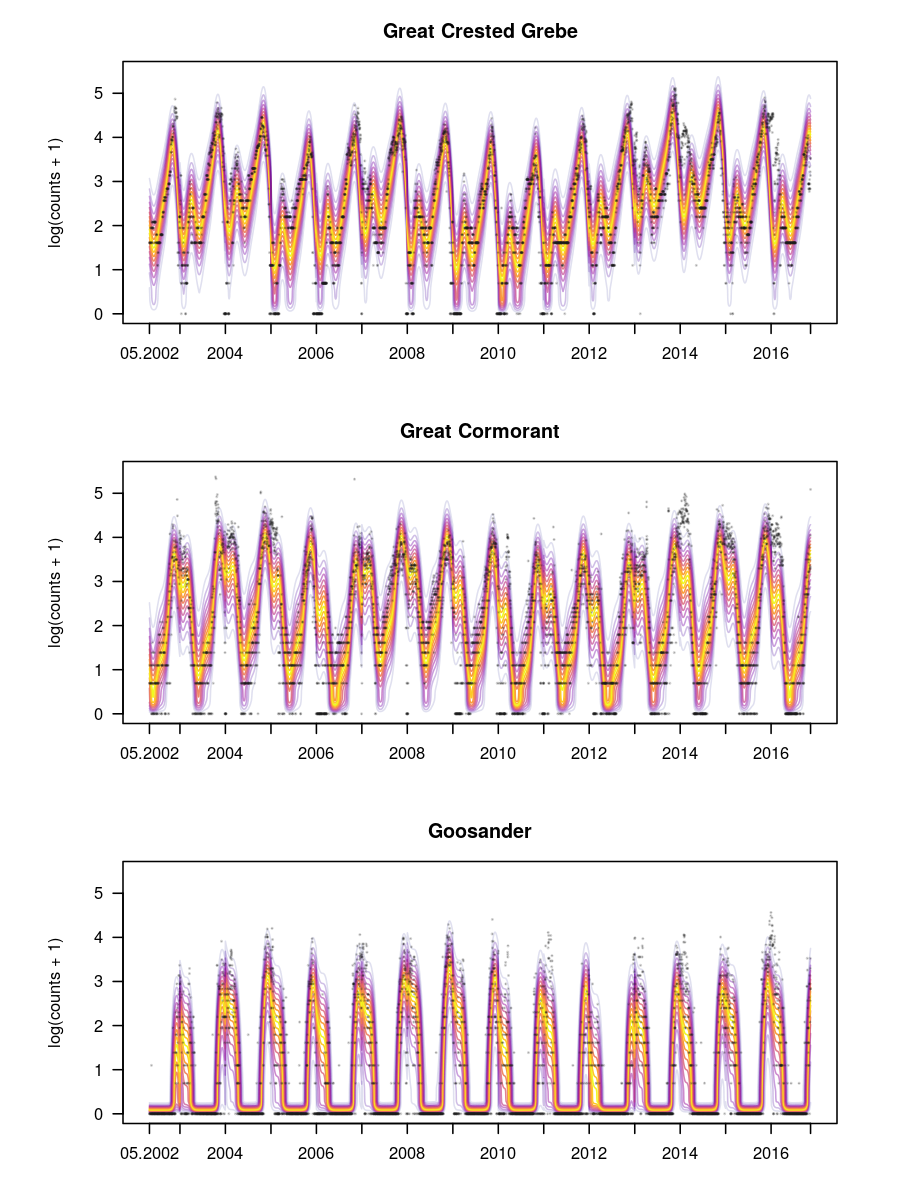
Figure 6: Model $\text{M-}\mathbf{\Lambda}(\text{\boldmath$x$})$, discrete approximation: univariate marginal distributions conditional on time for the three bird species.

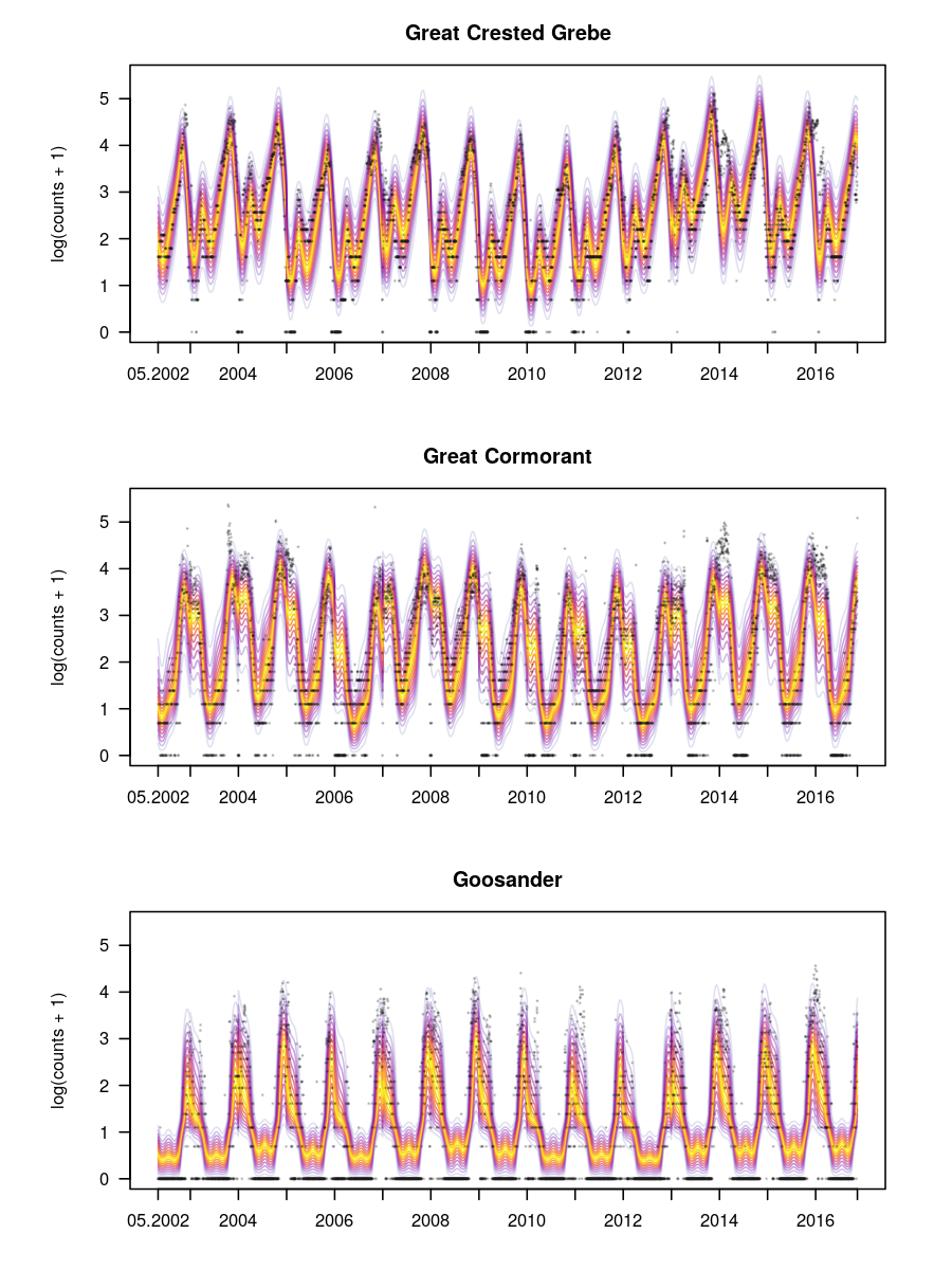
Figure 7: Model $\text{M-}\mathbf{\Lambda}$, continuous approximation: univariate marginal distributions conditional on time for the three bird species.

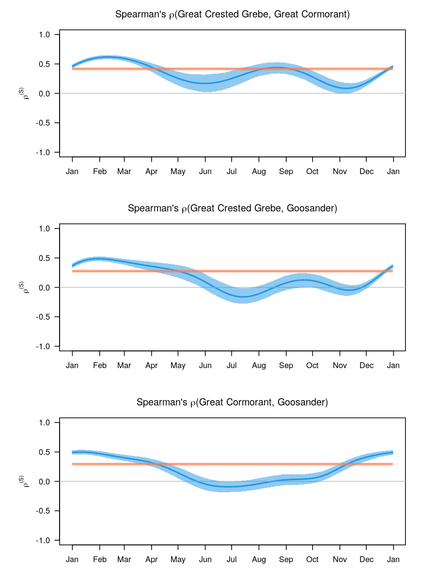
Figure 9: Model $\text{M-}\mathbf{\Lambda}(\text{\boldmath$x$})$, continuous approximation: trajectories of the pairwise Spearman’s rank correlations $\rho^{(S)}$ across species on a latent scale over one year and the corresponding 95% confidence intervals based on the asymptotic distribution of the parameters. For comparison, the constant Spearman’s rank correlations of model $\text{M-}\mathbf{\Lambda}$ (see Table 1) are plotted in orange with 95% confidence intervals.

For the continuous approximation, the log-likelihoods are $-41233.2$ for $\text{M-}\mathbf{\Lambda}$ and $-41038.9$ for $\text{M-}\mathbf{\Lambda}(\text{\boldmath$x$})$. Since the more complex model $\text{M-}\mathbf{\Lambda}(\text{\boldmath$x$})$ has $18$ parameters more than model $\text{M-}\mathbf{\Lambda}$, we compare twice the difference of the log-likelihoods of $\text{M-}\mathbf{\Lambda}(\text{\boldmath$x$})$ and $\text{M-}\mathbf{\Lambda}$ with a one-sided chi-squared distribution with 18 degrees of freedom and obtain strong evidence ($p<0.0001$) in favor of the more complex model $\text{M-}\mathbf{\Lambda}(\text{\boldmath$x$})$.

A.5 Comparison of the two approximations

How the two approximations of the likelihood affect the estimated parameters and model quality was investigated by a parametric bootstrap experiment.

New count observations were generated from a model estimated by the continuous approximation (leading to a maximum likelihood estimate $\text{\boldmath$\hat{\theta}$}_{\text{ML}}^{\text{(cont)}}$). For these artificial counts, the log-likelihood of the continuous approximation (Section 2.3.2) and the exact log-likelihood (Equation 8) are evaluated as a function of the artificial data and the parameters $\text{\boldmath$\hat{\theta}$}_{\text{ML}}^{\text{(cont)}}$ are used to generate the data. Similarly, new data are generated from the same model but using the discrete version $\text{\boldmath$\hat{\theta}$}_{\text{ML}}^{\text{(disc)}}$ and evaluating the log-likelihood of the discrete approximation (Section 2.3.3) and the exact log-likelihood.

For 50 bootstrap samples, the log-likelihood of the continuous approximation (Section 2.3.2) (Equation 8) the parameters $\text{\boldmath$\hat{\theta}$}_{\text{ML}}^{\text{(cont)}}$ were plotted and are shown in the left panel of Figure 10. In the right panel, the log-likelihood of the discrete approximation (Section 2.3.3) $\text{M-}\mathbf{\Lambda}$, estimated by the discrete version $\text{\boldmath$\hat{\theta}$}_{\text{ML}}^{\text{(disc)}}$. The agreement between the discrete approximation and the exact log-likelihood was relatively close. However, the continuous approximation performed slightly worse and generally resulted in slightly higher values of the exact log-likelihood.

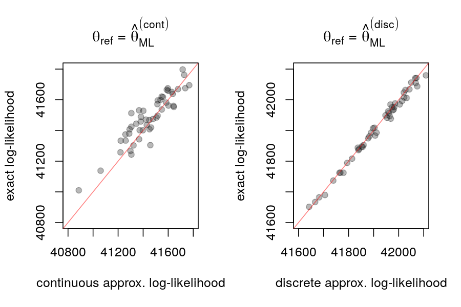
Figure 10: Scatter plots of the results of the parametric bootstrap (continuous approximation on the left, discrete approximation on the right). The red line denotes the identity of the exact and the approximated log-likelihood.

A.6 Sensitivity of the two approximations on species ordering

To illustrate the problem that arises when considering non-constant parameters $\mathbf{\Lambda}(\text{\boldmath$x$})$ in the inverse Cholesky factor (Section 4), we consider $(Y_{1},Y_{2})\sim\operatorname{N}_{2}(0,\mathbf{\Sigma}(x))$ with

$$\mathbf{\Lambda}(x)=\left(\begin{array}[]{cc}1&0\\ x&1\end{array}\right)\text{ and }\mathbf{\Sigma}(x)=\left(\begin{array}[]{cc}1&-x\\ -x&1+x^{2}\end{array}\right).$$

This situation is a special case of our model, with $\tilde{h}_{1}(y_{1})=y_{1}$ and $\tilde{h}_{2}(y_{2})=y_{2}$ but the model’s parameters can be estimated when applied to data $(Y_{1},Y_{2})$. Application of the model to the reversed data $(Y_{2},Y_{1})$ however fails, because the structure of $\mathbf{\Lambda}$ only allows an $x$-dependent variance in the second species. This is of course counter intuitive, as one would expect the correlations to be invariant with respect to species ordering. This issue can be addressed by introducing a dependency on $x$ into the transformation functions $\tilde{h}_{j},j=1,2$. Another option is to consider all possible species permutations and then choose the one that maximizes the likelihood. It may also help to understand the model as a directed acyclic graph (DAG), in which the correlation structure is dependent on habitat variables $x$. This issue was also noted by van der Wurp et al. (2020) and the authors suggested that the regression coefficients of the marginal models be penalized to ensure that the marginal effects are the same for all species. Otherwise, the order in which the marginal models are specified could influence the resulting parameter estimates.

A.7 An alternative to the continuous approximation

There are two alternatives regarding how much to subtract when transforming counts according to Equation 9. First, one can subtract any fixed amount in the interval $(0,1)$. This does not influence estimates of Spearman’s rhos between species but can have an influence on the value of the log-likelihood (however, still in a predictable manner). The second option would be to subtract a uniformly distributed random variable in $(0,1)$. The continuous extension (Schriever, 1986; Denuit and Lambert, 2005) of the $j$-th component of $Y$ is defined as $Y_{j}^{*}=Y_{j}-U_{j}$ for the amount of i.i.d uniform noise $U_{j}\sim\text{U}(0,1)$, $U_{j}$ independent of $Y_{j}$ for all $j=1,\dots,J$. At least on a univariate level, it can be shown that the transformation model obtained for any of the $Y_{j}^{*}$’s is valid for the original response $Y_{j}$, $j=1,\dots,J$. The resulting response vector $\text{\boldmath$Y$}^{*}$ is thus a jittered, continuous version of the original response vector $Y$. In theory, one could again apply the approach of Klein et al. (2020) and then “average out” (Machado and Silva, 2005) the random uniform noise in order to obtain a valid parameter estimate $\hat{\text{\boldmath$\theta$}}$ (Heinen and Rengifo, 2007, 2008) by refitting the model several times with different instances of the uniform noise $U$. However, Nikoloulopoulos (2013) showed that this approach usually underestimates both latent correlations and standard errors for the regression parameters, because the univariate, independent jittering that is applied component-wise does not account for the dependence already present in the data. An alternative approach to deal with the introduction of uniform jittering without underestimating the parameters is to maximize the so-called simulated likelihood (Nikoloulopoulos, 2013), but this is a topic for future research.

References

- Bakker et al. (2006) Elisabeth S Bakker, Mark E Ritchie, Han Olff, Daniel G Milchunas, and Johannes MH Knops. Herbivore impact on grassland plant diversity depends on habitat productivity and herbivore size. Ecology Letters, 9(7):780–788, 2006. doi: 10.1111/j.1461-0248.2006.00925.x.
- Cecala et al. (2020) Kristen K Cecala, Eli H Walker, Joshua R Ennen, Shawna M Fix, and Jon M Davenport. Seasonal variation in the strength of interference competition among headwater stream predators. Freshwater Biology, 65(8):1440–1449, 2020. doi: 10.1111/fwb.13511.
- De Felipe et al. (2019) Miguel De Felipe, Pedro Sáez-Gómez, and Carlos Camacho. Environmental factors influencing road use in a nocturnal insectivorous bird. European Journal of Wildlife Research, 65(3):31, 2019. doi: 10.1007/s10344-019-1267-5.
- Dean et al. (2017) Angela Dean, Daniel Voss, and Danel Draguljić. Design and Analysis of Experiments. Springer Texts in Statistics. Springer International Publishing, 2nd edition, 2017. doi: 10.1007/978-3-319-52250-0.
- De’ath (2002) Glenn De’ath. Multivariate regression trees: A new technique for modelling species-environment relationships. Ecology, 83(4):1105–1117, 2002. doi: 10.1890/0012-9658(2002)083[1105:MRTANT]2.0.CO;2.
- Denuit and Lambert (2005) Michel Denuit and Philippe Lambert. Constraints on concordance measures in bivariate discrete data. Journal of Multivariate Analysis, 93(1):40–57, 2005. doi: 10.1016/j.jmva.2004.01.004.
- Elith et al. (2008) Jane Elith, John R. Leathwick, and Trevor Hastie. A working guide to boosted regression trees. Journal of Animal Ecology, 77(4):802–813, 2008. doi: 10.1111/j.1365-2656.2008.01390.x.
- Gotelli and Ellison (2013) Nicholas J Gotelli and Aaron M Ellison. A Primer of Ecological Statistics. Sinauer Associates, Sunderland, MA, U.S.A., 2nd edition, 2013.
- Heinen and Rengifo (2007) Andréas Heinen and Erick Rengifo. Multivariate autoregressive modeling of time series count data using copulas. Journal of Empirical Finance, 14(4):564–583, 2007. doi: 10.1016/j.jempfin.2006.07.004.
- Heinen and Rengifo (2008) Andréas Heinen and Erick Rengifo. Multivariate reduced rank regression in non-Gaussian contexts, using copulas. Computational Statistics & Data Analysis, 52(6):2931–2944, 2008. doi: 10.1016/j.csda.2007.08.012.
- Held and Paul (2012) Leonhard Held and Michaela Paul. Modeling seasonality in space-time infectious disease surveillance data. Biometrical Journal, 54(6):824–843, 2012. doi: 10.1002/bimj.20120003.
- Hothorn (2020) Torsten Hothorn. Most likely transformations: The mlt package. Journal of Statistical Software, 92(1):1–68, 2020. doi: 10.18637/jss.v092.i01.
- Hothorn and Barbanti (2022) Torsten Hothorn and Luisa Barbanti. tram: Transformation Models, 2022. URL https://R-Forge.R-project.org/projects/ctm/. R package version 0.7-0/r1776.
- Hothorn et al. (2011) Torsten Hothorn, Jörg Müller, Boris Schröder, Thomas Kneib, and Roland Brandl. Decomposing environmental, spatial, and spatiotemporal components of species distributions. Ecological Monographs, 81(2):329–347, 2011. doi: 10.1890/10-0602.1.
- Hothorn et al. (2018) Torsten Hothorn, Lisa Möst, and Peter Bühlmann. Most likely transformations. Scandinavian Journal of Statistics, 45(1):110–134, 2018. doi: 10.1111/sjos.12291.
- Ingram et al. (2020) Martin Ingram, Damjan Vukcevic, and Nick Golding. Multi-output Gaussian processes for species distribution modelling. Methods in Ecology and Evolution, 11(12):1587–1598, 2020. doi: 10.1111/2041-210X.13496.
- Ives (2015) Anthony R. Ives. For testing the significance of regression coefficients, go ahead and log-transform count data. Methods in Ecology and Evolution, 6(7):828–835, 2015. doi: 10.1111/2041-210X.12386.
- Ives and Helmus (2011) Anthony R. Ives and Matthew R. Helmus. Generalized linear mixed models for phylogenetic analyses of community structure. Ecological Monographs, 81(3):511–525, 2011. doi: 10.1890/10-1264.1.
- Kinshofer et al. (2018) Gerhard Kinshofer, Roland Brandl, and Robert Pfeifer. Keine Hinweise auf Konkurrenz zwischen Kormoran Phalacrocorax carbo, Haubentaucher Podiceps cristatus und Gänsesäger Mergus merganser. Ornithol. Anz., 56:132–143, 2018.
- Kissling et al. (2012) W. Daniel Kissling, Carsten F. Dormann, Jürgen Groeneveld, Thomas Hickler, Ingolf Kühn, Greg J. McInerny, José M. Montoya, Christine Römermann, Katja Schiffers, Frank M. Schurr, Alexander Singer, Jens-Christian Svenning, Niklaus E. Zimmermann, and Robert B. O’Hara. Towards novel approaches to modelling biotic interactions in multispecies assemblages at large spatial extents. Journal of Biogeography, 39(12):2163–2178, 2012. doi: 10.1111/j.1365-2699.2011.02663.x.
- Klein et al. (2020) Nadja Klein, Torsten Hothorn, Luisa Barbanti, and Thomas Kneib. Multivariate conditional transformation models. Scandinavian Journal of Statistics, 2020. doi: 10.1002/sjos.12501.
- Lee and Nelder (2004) Youngjo Lee and John A Nelder. Conditional and marginal models: Another view. Statistical Science, 19(2):219–238, 2004. doi: 10.1214/088342304000000305.
- Machado and Silva (2005) José A F Machado and JMC Santos Silva. Quantiles for counts. Journal of the American Statistical Association, 100(472):1226–1237, 2005. doi: 10.1198/016214505000000330.
- Mooney et al. (2016) Emily H Mooney, Joseph S Phillips, Chadwick V Tillberg, Cheryl Sandrow, Annika S Nelson, and Kailen A Mooney. Abiotic mediation of a mutualism drives herbivore abundance. Ecology Letters, 19(1):37–44, 2016. doi: 10.1111/ele.12540.
- Muff et al. (2016) Stefanie Muff, Leonhard Held, and Lukas F. Keller. Marginal or conditional regression models for correlated non-normal data? Methods in Ecology and Evolution, 7(12):1514–1524, 2016. doi: 10.1111/2041-210X.12623.
- Nikoloulopoulos (2013) Aristidis K Nikoloulopoulos. On the estimation of normal copula discrete regression models using the continuous extension and simulated likelihood. Journal of Statistical Planning and Inference, 143(11):1923–1937, 2013. doi: 10.1016/j.jspi.2013.06.015.
- Norberg et al. (2019) Anna Norberg, Nerea Abrego, F Guillaume Blanchet, Frederick R Adler, Barbara J Anderson, Jani Anttila, Miguel B Araújo, Tad Dallas, David Dunson, Jane Elith, et al. A comprehensive evaluation of predictive performance of 33 species distribution models at species and community levels. Ecological Monographs, 89(3), 2019. doi: 10.1002/ecm.1370.
- Ovaskainen and Soininen (2011) Otso Ovaskainen and Janne Soininen. Making more out of sparse data: Hierarchical modeling of species communities. Ecology, 92(2):289–295, 2011. doi: 10.1890/10-1251.1.
- Ovaskainen et al. (2010) Otso Ovaskainen, Jenni Hottola, and Juha Siitonen. Modeling species co-occurrence by multivariate logistic regression generates new hypotheses on fungal interactions. Ecology, 91(9):2514–2521, 2010. doi: 10.1890/10-0173.1.
- Ovaskainen et al. (2017) Otso Ovaskainen, Gleb Tikhonov, Anna Norberg, F Guillaume Blanchet, Leo Duan, David Dunson, Tomas Roslin, and Nerea Abrego. How to make more out of community data? A conceptual framework and its implementation as models and software. Ecology Letters, 20(5):561–576, 2017. doi: 10.1111/ele.12757.
- Petren and Case (1998) Kenneth Petren and Ted J Case. Habitat structure determines competition intensity and invasion success in gecko lizards. Proceedings of the National Academy of Sciences, 95(20):11739–11744, 1998. doi: 10.1073/pnas.95.20.11739.
- Pollock et al. (2014) Laura J. Pollock, Reid Tingley, William K. Morris, Nick Golding, Robert B. O’Hara, Kirsten M. Parris, Peter A. Vesk, and Michael A. McCarthy. Understanding co-occurrence by modelling species simultaneously with a Joint Species Distribution Model (JSDM). Methods in Ecology and Evolution, 5(5):397–406, 2014. doi: 10.1111/2041-210X.12180.
- R Core Team (2021) R Core Team. R: A Language and Environment for Statistical Computing. R Foundation for Statistical Computing, Vienna, Austria, 2021. URL https://www.R-project.org/.
- Schriever (1986) Bert F Schriever. Order Dependence, volume 20. Centrum voor Wiskunde en Informatica Amsterdam, Amsterdam, The Netherlands, 1986.
- Siegfried and Hothorn (2020) Sandra Siegfried and Torsten Hothorn. Count transformation models. Methods in Ecology and Evolution, 11(7):818–827, 2020. doi: 10.1111/2041-210X.13383.
- Siegfried et al. (2022) Sandra Siegfried, Luisa Barbanti, and Torsten Hothorn. cotram: Count Transformation Models, 2022. URL http://ctm.R-forge.R-project.org. R package version 0.3-2.
- Suter (1995) Werner Suter. Are Cormorants Phalacrocorax carbo wintering in Switzerland approaching carrying capacity? An analysis of increase patterns and habitat choice. Ardea, 83(1):255–266, 1995.
- Tamási and Hothorn (2021) Bálint Tamási and Torsten Hothorn. tramME: Mixed-effects transformation models using template model builder. The R Journal, 2021. URL https://cran.r-project.org/web/packages/tramME/vignettes/tramME.pdf. Accepted for publication 2021-08-16.
- Tamási et al. (2022) Bálint Tamási, Michael Crowther, Milo Alan Puhan, Ewout Steyerberg, and Torsten Hothorn. Individual participant data meta-analysis with mixed-effects transformation models. Biostatistics, 2022. doi: 10.1093/biostatistics/kxab045.
- Thas et al. (2012) Olivier Thas, Jan De Neve, Lieven Clement, and Jean-Pierre Ottoy. Probabilistic index models. Journal of the Royal Statistical Society: Series B (Statistical Methodology), 74(4):623–671, 2012. doi: 10.1111/j.1467-9868.2011.01020.x.
- Tikhonov et al. (2017) Gleb Tikhonov, Nerea Abrego, David Dunson, and Otso Ovaskainen. Using joint species distribution models for evaluating how species-to-species associations depend on the environmental context. Methods in Ecology and Evolution, 8(4):443–452, 2017. doi: 10.1111/2041-210X.12723.
- Tikhonov et al. (2021) Gleb Tikhonov, Otso Ovaskainen, Jari Oksanen, Melinda de Jonge, Oystein Opedal, and Tad Dallas. Hmsc: Hierarchical Model of Species Communities, 2021. URL https://CRAN.R-project.org/package=Hmsc. R package version 3.0-11.
- van der Wurp et al. (2020) Hendrik van der Wurp, Andreas Groll, Thomas Kneib, Giampiero Marra, and Rosalba Radice. Generalised joint regression for count data: a penalty extension for competitive settings. Statistics and Computing, 30(5):1419–1432, 2020. doi: 10.1007/s11222-020-09953-7.
- Warton et al. (2015) David I. Warton, F. Guillaume Blanchet, Robert B. O’Hara, Otso Ovaskainen, Sara Taskinen, Steven C. Walker, and Francis K.C. Hui. So many variables: Joint modeling in community ecology. Trends in Ecology & Evolution, 30(12):766–779, 2015. doi: 10.1016/j.tree.2015.09.007.
- Wignall et al. (2020) Veronica R Wignall, Isabella Campbell Harry, Natasha L Davies, Stephen D Kenny, Jack K McMinn, and Francis LW Ratnieks. Seasonal variation in exploitative competition between honeybees and bumblebees. Oecologia, 192(2):351–361, 2020. doi: 10.1007/s00442-019-04576-w.