Inductive Matrix Completion:
No Bad Local Minima and a Fast Algorithm

Abstract

The inductive matrix completion (IMC) problem is to recover a low rank matrix from few observed entries while incorporating prior knowledge about its row and column subspaces. In this work, we make three contributions to the IMC problem: (i) we prove that under suitable conditions, the IMC optimization landscape has no bad local minima; (ii) we derive a simple scheme with theoretical guarantees to estimate the rank of the unknown matrix; and (iii) we propose GNIMC, a simple Gauss-Newton based method to solve the IMC problem, analyze its runtime and derive recovery guarantees for it. The guarantees for GNIMC are sharper in several aspects than those available for other methods, including a quadratic convergence rate, fewer required observed entries and stability to errors or deviations from low-rank. Empirically, given entries observed uniformly at random, GNIMC recovers the underlying matrix substantially faster than several competing methods.

1 Introduction

In low rank matrix completion, a well-known problem that appears in various applications, the task is to recover a rank-$r$ matrix $X^{*}\in\mathbb{R}^{n_{1}\times n_{2}}$ given few of its entries, where $r\ll\min\{n_{1},n_{2}\}$. In the problem of inductive matrix completion (IMC), beyond being low rank, $X^{*}$ is assumed to have additional structure as follows: its columns belong to the range of a known matrix $A\in\mathbb{R}^{n_{1}\times d_{1}}$ and its rows belong to the range of a known matrix $B\in\mathbb{R}^{n_{2}\times d_{2}}$, where $r\leq d_{1}\leq n_{1}$ and $r\leq d_{2}\leq n_{2}$. Hence, $X^{*}$ may be written as $X^{*}=AM^{*}B^{\top}$, and the task reduces to finding the smaller matrix $M^{*}\in\mathbb{R}^{d_{1}\times d_{2}}$. In practice, the low rank and/or the additional structure assumptions may hold only approximately, and in addition, the observed entries may be corrupted by noise.

The side information matrices $A,B$ may be viewed as feature representations. For example, in movies recommender systems, the task is to complete a matrix $X^{*}$ of the ratings given by $n_{1}$ users to $n_{2}$ movies. The columns of $A,B$ may correspond to viewers’ demographic details (age, gender) and movies’ properties (length, genre), respectively [ABEV09, MCG⁺11, CZL⁺12, YL19]. The underlying assumption in IMC is that uncovering the relations between the viewers and the movies in the feature space, as encoded in $M^{*}$, suffices to deduce the ratings $X^{*}=AM^{*}B^{\top}$. Other examples of IMC include multi-label learning [XJZ13, SCH⁺16, ZDG18], disease prediction from gene/miRNA/lncRNA data [ND14, CWQ⁺18, LYL⁺18] and link prediction in networks [ME11, CDH18].

If the side information matrices allow for a significant dimensionality reduction, namely $d\ll n$ where $d=\max\{d_{1},d_{2}\}$ and $n=\max\{n_{1},n_{2}\}$, recovering $X^{*}$ is easier from both theoretical and computational perspectives. From the information limit aspect, the minimal number of observed entries required to complete a matrix of rank $r$ with side information scales as $\mathcal{O}(dr)$, compared to $\mathcal{O}(nr)$ without side information. Similarly, the number of variables scale as $d$ rather than as $n$, enabling more efficient computation and less memory. Finally, features also allow completion of rows and columns of $X^{*}$ that do not have even a single observed entry. Unlike standard matrix completion which requires at least $r$ observed entries in each row and column of $X^{*}$, in IMC the feature vector is sufficient to inductively predict the full corresponding row/column; hence the name ’Inductive Matrix Completion’.

Table 1: Recovery guarantees for the algorithms: Maxide [XJZ13], AltMin [JD13], MPPF [ZDG18] and GNIMC (this work), for an $n\times n$ matrix $X^{*}$ of rank $r$ and condition number $\kappa$, and $d\times d$ side information matrices of incoherence $\mu$, given a fixed target accuracy. Here $f(\kappa,\mu)$ is some function of $\kappa$ and $\mu$. For a more detailed comparison, see Section 5.2.

Algorithm	Sample complexity $|\Omega|\gtrsim...$	Requires incoherent $X^{*}$?	Error decay rate	Time complexity $\sim\mathcal{O}(...)$
Maxide	$\mu^{2}dr[1+\log(d/r)]\log n$	yes	unspecified	unspecified
AltMin	$\kappa^{2}\mu^{4}d^{2}r^{3}\log n$	no	unspecified	unspecified
MPPF	$(\kappa r+d)\kappa^{2}\mu^{2}r^{2}\log d\log n$	yes	linear	$f(\kappa,\mu)\cdot n^{3/2}d^{2}r^{3}\log d\log n$
GNIMC (ours)	$\mu^{2}d^{2}\log n$	no	quadratic	$\mu^{2}d^{3}r\log n$

Several IMC methods were devised in the past years. Perhaps the most popular ones are nuclear norm minimization [XJZ13, LYL⁺18] and alternating minimization [JD13, ND14, ZJD15, CWQ⁺18]. Another recent method is multi-phase Procrustes flow [ZDG18]. While nuclear norm minimization enjoys strong recovery guarantees, it is computationally slow. Other methods are faster, but the number of observed entries for their recovery guarantees to hold depends on the condition number of $X^{*}$.

In this work, we make three contributions to the IMC problem. First, by deriving an RIP (Restricted Isometry Property) guarantee for IMC, we prove that under certain conditions the optimization landscape of IMC is benign (Theorem 3.1). Compared to a similar result derived in [GSG18], our guarantee requires significantly milder conditions, and in addition, addresses the vanilla IMC problem rather than a suitably regularized one.

Second, we propose a simple scheme to estimate the rank of $X^{*}$ from its observed entries and the side information matrices $A,B$. We also provide a theoretical guarantee for the accuracy of the estimated rank (Theorem 4.1), which holds for either exactly or approximately low rank $X^{*}$ and with noisy measurements.

Third, we propose a simple Gauss-Newton based method to solve the IMC problem, that is both fast and enjoys strong recovery guarantees. Our algorithm, named GNIMC (Gauss-Newton IMC), is an adaptation of the GNMR algorithm [ZN22] to IMC. At each iteration, GNIMC solves a least squares problem; yet, its per-iteration complexity is of the same order as gradient descent. As a result, empirically, our tuning-free GNIMC implementation is 2 to 17 times faster than competing algorithms in various settings, including ill-conditioned matrices and very few observations, close to the information limit.

On the theoretical front, we prove that given a standard incoherence assumption on $A,B$ and sufficiently many observed entries sampled uniformly at random, GNIMC recovers $X^{*}$ at a quadratic convergence rate (Theorem 5.1). As far as we know, this is the only available quadratic convergence rate guarantee for any IMC algorithm. In addition, we prove that GNIMC is stable against small arbitrary additive error (Theorem 5.4), which may originate from (i) inaccurate measurements of $X^{*}$, (ii) inaccurate side information, and/or (iii) $X^{*}$ being only approximately low rank.

Remarkably, our guarantees do not require $X^{*}$ to be incoherent, and the required number of observations depends only on properties of $A,B$ and not on those of $X^{*}$. Other guarantees have similar dependence on $A,B$, but in addition either depend on the condition number of $X^{*}$ and/or require incoherence of $X^{*}$, see Table 1. Relaxing the incoherence assumption on $X^{*}$ is important, since $X^{*}$ is only partially observed and such an assumption cannot be verified. In contrast, the matrices $A,B$ are known and their incoherence can be verified.

Notation. The $i$-th largest singular value of a matrix $X$ is denoted by $\sigma_{i}=\sigma_{i}(X)$. The condition number of a rank-$r$ matrix is denoted by $\kappa=\sigma_{1}/\sigma_{r}$. The $i$-th standard basis vector is denoted by $e_{i}$, and the Euclidean norm of a vector $x$ by $\|x\|$. The spectral norm of a matrix $X$ is denoted by $\|X\|_{2}$, its Frobenius norm by $\|X\|_{F}$, its largest row norm by $\|X\|_{2,\infty}\equiv\max_{i}\|X^{\top}e_{i}\|$, its largest entry magnitude by $\|X\|_{\infty}\equiv\max_{i,j}|X_{ij}|$, and the set of its column vectors by $\text{col}(X)$. A matrix $X$ is an isometry if $X^{\top}X=I$, where $I$ is the identity matrix. Denote by $\mathcal{P}_{AB}:\mathbb{R}^{n_{1}\times n_{2}}\to\mathbb{R}^{n_{1}\times n_{2}}$ the projection operator into the row and column spaces of $A,B$, respectively, such that $\mathcal{P}_{AB}(X)=AA^{\top}XBB^{\top}$ if $A,B$ are isometries. Denote by $\mathcal{P}_{\Omega}:\mathbb{R}^{n_{1}\times n_{2}}\to\mathbb{R}^{n_{1}\times n_{2}}$ the sampling operator that projects a matrix in $\mathbb{R}^{n_{1}\times n_{2}}$ onto an observation set $\Omega\subseteq[n_{1}]\times[n_{2}]$, such that $[\mathcal{P}_{\Omega}(X)]_{ij}=X_{ij}$ if $(i,j)\in\Omega$ and $0$ otherwise. Denote by $\text{Vec}_{\Omega}(X)\in\mathbb{R}^{|\Omega|}$ the vector with the entries $X_{ij}$ for all $(i,j)\in\Omega$. Finally, denote by $p=|\Omega|/(n_{1}n_{2})$ the sampling rate of $\Omega$.

2 Problem Formulation

Let $X^{*}\in\mathbb{R}^{n_{1}\times n_{2}}$ be a matrix of rank $r$. For now we assume $r$ is known; in Section 4 we present a scheme to estimate $r$, and prove its accuracy. Assume $\Omega\subseteq[n_{1}]\times[n_{2}]$ is uniformly sampled and known, and let $Y=\mathcal{P}_{\Omega}(X^{*}+\mathcal{E})$ be the observed matrix where $\mathcal{E}$ is additive error. In the standard matrix completion problem, the goal is to solve

$$\min_{X}\|\mathcal{P}_{\Omega}(X)-Y\|_{F}^{2}\quad\text{s.t. }\text{rank}(X)\leq r.$$ (MC)

In IMC, in addition to the observations $Y$ we are given two side information matrices $A\in\mathbb{R}^{n_{1}\times d_{1}}$ and $B\in\mathbb{R}^{n_{2}\times d_{2}}$ with $r\leq d_{i}\leq n_{i}$ for $i=1,2$, such that

$$\text{col}(X^{*})\subseteq\text{span col}(A),\;\;\text{col}(X^{*\top})\subseteq\text{span col}(B).$$ (1)

Note that w.l.o.g., we may assume that $A$ and $B$ are isometries, $A^{\top}A=I_{d_{1}}$ and $B^{\top}B=I_{d_{2}}$, as property (1) is invariant to orthonormalization of the columns of $A$ and $B$. Standard matrix completion corresponds to $d_{i}=n_{i}$ with the trivial side information $A=I_{n_{1}}$, $B=I_{n_{2}}$. A common assumption in IMC is $d_{i}\ll n_{i}$, so that the side information is valuable. Note that beyond allowing for (potentially adversarial) inaccurate measurements, $\mathcal{E}$ may also capture violations of the low rank and the side information assumption (1), as we can view $X^{*}+\mathcal{E}$ as the true underlying matrix whose only first component, $X^{*}$, has exact low rank and satisfies (1).

Assumption (1) implies that $X^{*}=AM^{*}B^{\top}$ for some rank-$r$ matrix $M^{*}\in\mathbb{R}^{d_{1}\times d_{2}}$. The IMC problem thus reads

$$\min_{M}\|\mathcal{P}_{\Omega}(AMB^{\top})-Y\|_{F}^{2}\quad\text{s.t. }\text{rank}(M)\leq r.$$ (IMC)

Some works on IMC [XJZ13, ZDG18] assume that both $X^{*}$ and $A,B$ are incoherent, namely have small incoherence, defined as follows [CR09, KMO10].

Definition 2.1 ($\mu$-incoherence).

A matrix $X\in\mathbb{R}^{n_{1}\times n_{2}}$ of rank $r$ is $\mu$-incoherent if its Singular Value Decomposition (SVD), $U\Sigma V^{\top}$ with $U\in\mathbb{R}^{n_{1}\times r}$ and $V\in\mathbb{R}^{n_{2}\times r}$, satisfies

$$\|U\|_{2,\infty}\leq\sqrt{\mu r/n_{1}}\,\,\mbox{ and }\,\|V\|_{2,\infty}\leq\sqrt{\mu r/n_{2}}.$$

However, for IMC to be well-posed, $X^{*}$ does not have to be incoherent, and it suffices for $A,B$ to be incoherent [JD13]. In case $A$ and $B$ are isometries, their incoherence assumption corresponds to bounded row norms, $\|A\|_{2,\infty}\leq\sqrt{\mu d_{1}/n_{1}}$ and $\|B\|_{2,\infty}\leq\sqrt{\mu d_{2}/n_{2}}$.

3 No Bad Local Minima Guarantee

In this section we present a novel characterization of the optimization landscape of IMC. Following the factorization approach to matrix recovery problems, we first incorporate the rank constraint into the objective by writing the unknown matrix as $M=UV^{\top}$ where $U\in\mathbb{R}^{d_{1}\times r}$ and $V\in\mathbb{R}^{d_{2}\times r}$. Then, problem (IMC) is

$$\min_{U,V}\|\mathcal{P}_{\Omega}(AUV^{\top}B^{\top})-Y\|_{F}^{2}.$$ (2)

Clearly, any pair of matrices $(U,V)$ whose product is $UV^{\top}=M^{*}$ is a global minimizer of (2) with an objective value of zero. However, as (2) is non-convex, some of its first-order critical points, namely points at which the gradient vanishes, may be bad local minima. The next result, proven in Appendix C, states that if sufficiently many entries are observed, all critical points are either global minima or strict saddle points. At a strict saddle point the Hessian has at least one strictly negative eigenvalue, so that gradient descent will not reach it. Hence, under the conditions of Theorem 3.1, gradient descent will recover $M^{*}$ from a random initialization.

Theorem 3.1.

Let $X^{*}\in\mathbb{R}^{n_{1}\times n_{2}}$ be a rank-$r$ matrix which satisfies (1) with $\mu$-incoherent matrices $A\in\mathbb{R}^{n_{1}\times d_{1}}$ and $B\in\mathbb{R}^{n_{2}\times d_{2}}$. Assume $\Omega\subseteq[n_{1}]\times[n_{2}]$ is uniformly sampled with $|\Omega|\gtrsim\mu^{2}d_{1}d_{2}\log n$. Then w.p. at least $1-2n^{-2}$, any critical point $(U,V)$ of problem (2) is either a global minimum with $UV^{\top}=M^{*}$, or a strict saddle point.

To the best of our knowledge, Theorem 3.1 is the first guarantee for the geometry of vanilla IMC. A previous result by [GSG18] only addressed a suitably balance-regularized version of (2). In addition, their guarantee requires $\mathcal{O}(\mu^{2}r\max\{d_{1},d_{2}\}\max\{d_{1}d_{2},\log^{2}n\})$ observed entries with cubic scaling in $d_{1},d_{2}$, which is significantly larger than the quadratic scaling in our Theorem 3.1.

Theorem 3.1 guarantees exact recovery for a family of algorithms beyond vanilla gradient descent. However, as illustrated in Section 6, solving the IMC problem can be done much faster than by gradient descent or variants thereof, e.g. by our proposed GNIMC method described in Section 5.

3.1 IMC as a special case of matrix sensing

Similar to [GSG18], our proof of Theorem 3.1 is based on an RIP result we derive for IMC. The RIP result forms a connection between IMC and the matrix sensing (MS) problem, as follows. Recall that in IMC, the goal is to recover $M^{*}\in\mathbb{R}^{d_{1}\times d_{2}}$ from the observations $Y=\mathcal{P}_{\Omega}(AM^{*}B^{\top}+\mathcal{E})$. In MS, we observe a set of linear measurements $b\equiv\mathcal{A}(M^{*})+\xi$ where $\mathcal{A}:\mathbb{R}^{d_{1}\times d_{2}}\to\mathbb{R}^{m}$ is a sensing operator and $\xi\in\mathbb{R}^{m}$ is additive error. Assuming a known or estimated rank $r$ of $M^{*}$, the goal is to solve

$$\min_{M}\|\mathcal{A}(M)-b\|^{2}\quad \text{s.t. }\text{rank}(M)\leq r.$$ (MS)

Problem (IMC) is in the form of (MS) with the operator

$$\mathcal{A}(M)=\text{Vec}_{\Omega}(AMB^{\top})/\sqrt{p}$$ (3)

and the error vector $\xi=\text{Vec}_{\Omega}(\mathcal{E})/\sqrt{p}$. However, unlike IMC, in MS the operator $\mathcal{A}$ is assumed to satisfy a suitable RIP (Restricted Isometry Property), defined as follows [Can08, RFP10].

Definition 3.2.

A linear map $\mathcal{A}:\mathbb{R}^{d_{1}\times d_{2}}\to\mathbb{R}^{m}$ satisfies a $k$-RIP with a constant $\delta\in[0,1)$, if for all matrices $M\in\mathbb{R}^{d_{1}\times d_{2}}$ of rank at most $k$,

$$(1-\delta)\|M\|_{F}^{2}\leq\|\mathcal{A}(M)\|^{2}\leq(1+\delta)\|M\|_{F}^{2}.$$ (4)

The following theorem, proven in Appendix A, states that if $A,B$ are incoherent and $|\Omega|$ is sufficiently large, w.h.p. the IMC sensing operator (3) satisfies the RIP. This observation creates a bridge between IMC and MS: for a given MS method, its RIP-based theoretical guarantees can be directly transferred to IMC.

Theorem 3.3.

Let $A\in\mathbb{R}^{n_{1}\times d_{1}}$, $B\in\mathbb{R}^{n_{2}\times d_{2}}$ be two isometry matrices such that $\|A\|_{2,\infty}\leq\sqrt{\mu d_{1}/n_{1}}$ and $\|B\|_{2,\infty}\leq\sqrt{\mu d_{2}/n_{2}}$. Let $\delta\in[0,1)$, and assume $\Omega\subseteq[n_{1}]\times[n_{2}]$ is uniformly sampled with $|\Omega|\equiv m\geq(8/\delta^{2})\mu^{2}d_{1}d_{2}\log n$. Then, w.p. at least $1-2n^{-2}$, the sensing operator $\mathcal{A}$ defined in (3) satisfies an RIP (4) with $k=\min\{d_{1},d_{2}\}$ and with constant $\delta$.

A similar result was derived in [GSG18]. Theorem 3.3 improves upon it both in terms of the required conditions and in terms of the RIP guarantee. First, as in their landscape guarantee, [GSG18] require cubic scaling with $d_{1},d_{2}$ rather than quadratic as in our result. Moreover, their sample complexity includes an additional factor of $r\log(1/\delta)$ (see Appendix F). Second, they proved only a $\min\{2r,d_{1},d_{2}\}$-RIP, whereas Theorem 3.3 guarantees that $\mathcal{A}$ satisfies the RIP with the maximal possible rank $\min\{d_{1},d_{2}\}$. In particular, this allows us to employ a recent result due to [LLZ⁺20] to prove Theorem 3.1 for vanilla IMC. The technical reason behind our sharper results is that instead of applying the Bernstein matrix inequality to a fixed matrix and then proving a union bound for all matrices, we apply it to a cleverly designed operator, which directly guarantees the result for all matrices (see Lemma A.1).

4 Rank Estimation Scheme

The factorization approach (2) requires knowing $r$ in advance, although in practice it is often unknown. In this section we propose a simple scheme to estimate the underlying rank, and provide a theoretical guarantee for it. Importantly, our scheme does not assume $X^{*}$ is exactly low rank, but rather the existence of a sufficiently large spectral gap between its $r$-th and $(r+1)$-th singular values.

Let $\hat{X}=\mathcal{P}_{AB}(Y)/p=AA^{\top}YBB^{\top}/p$ where $Y$ is the observed matrix and $p\equiv|\Omega|/(n_{1}n_{2})$, and denote its singular values by $\hat{\sigma}_{i}$. Our estimator for the rank of $X^{*}$ is

$$\hat{r} =\operatorname*{arg\,max}_{i}\,g_{i}(\hat{X}),\quad g_{i}(\hat{X})=\frac{\hat{\sigma}_{i}}{\hat{\sigma}_{i+1}+D\cdot\hat{\sigma}_{1}\sqrt{i}},$$ (5)

for some constant $D<1$. In our simulations we set $D=(\sqrt{d_{1}d_{2}}/|\Omega|)^{1/2}$. The function $g_{i}$ measures the $i$-th spectral gap, with the second term in the denominator added for robustness of the estimate. For $D=0$, $g_{i}$ is simply the ratio between two consecutive singular values. A similar estimator was proposed in [KMO09] for standard matrix completion, though they did not provide guarantees for it. The difference in our estimator is the incorporation of the side information matrices $A,B$. In addition, we present the following theoretical guarantee for our estimator, proven in Appendix B. Note that using the side information matrices $A,B$ allows us to reduce the sample complexity from $\mathcal{O}(n)$, as necessary in standard matrix completion, to only $\mathcal{O}(\log(n))$.

Theorem 4.1.

There exists a sufficiently small constant $c$ such that the following holds w.p. at least $1-2n^{-2}$. Let $X^{*}\in\mathbb{R}^{n_{1}\times n_{2}}$ be a matrix which satisfies (1) with $\mu$-incoherent $A,B$. Assume $X^{*}$ is approximately rank $r$, in the sense that for all $i\neq r$, $g_{r}(X^{*})>\min\{(11/10)g_{i}(X^{*}),1/10\}$. Denote $\delta=\min_{i}\{\sigma_{i+1}(X^{*})+D\sigma_{1}(X^{*})\sqrt{i}\}$, and assume $\Omega\subseteq[n_{1}]\times[n_{2}]$ is uniformly sampled with $|\Omega|\geq 8\mu^{2}d_{1}d_{2}\log(n)\|X\|_{F}^{2}/(c\delta)^{2}$. Further assume bounded error $\epsilon\equiv\|\mathcal{P}_{AB}\mathcal{P}_{\Omega}(\mathcal{E})\|_{F}/p\leq c\delta$. Then $\hat{r}=r$.

To the best of our knowledge, Theorem 4.1 is the first guarantee in the literature for rank estimation in IMC. We remark that with a suitably modified $\delta$, our guarantee holds for other choices of $g_{i}$ as well (including $g_{i}=\sigma_{i}/\sigma_{i+1}$, corresponding to $D=0$). An empirical demonstration of our scheme appears in Section 6.1.

5 GNIMC Algorithm

In this section, we describe an adaptation of the GNMR algorithm [ZN22] to IMC, and present recovery guarantees for it. Consider the factorized objective (2). Given an estimate $(U,V)$, the goal is to find an update $(\Delta U,\Delta V)$ such that $(U^{\prime},V^{\prime})=(U+\Delta U,V+\Delta V)$ minimizes (2). In terms of $(\Delta U,\Delta V)$, problem (2) reads

$$\min_{\Delta U,\Delta V}\| \mathcal{P}_{\Omega}(AUV^{\top}B^{\top}+AU\Delta V^{\top}B^{\top}+A\Delta UV^{\top}B^{\top}+A\Delta U\Delta V^{\top}B^{\top})-Y\|_{F}^{2},$$

which is nonconvex due to the mixed term $\Delta U\Delta V^{\top}$. The Gauss-Newton approach is to neglect this term. This yields the key iterative step of GNIMC, which is solving the following sub-problem:

$$\min_{\Delta U,\Delta V}\| \mathcal{P}_{\Omega}(AUV^{\top}B^{\top}+AU\Delta V^{\top}B^{\top}+A\Delta UV^{\top}B^{\top})-Y\|_{F}^{2}.$$ (6)

Problem (6) is a linear least squares problem. Note, however, that it has an infinite number of solutions: for example, if $(\Delta U,\Delta V)$ is a solution, so is $(\Delta U+UR,\Delta V-VR^{\top})$ for any $R\in\mathbb{R}^{r\times r}$. We choose the solution with minimal norm $\|\Delta U\|_{F}^{2}+\|\Delta V\|_{F}^{2}$, see Algorithm 1. In practice, this solution can be computed using the standard LSQR algorithm [PS82].

input :  sampling operator $\mathcal{P}_{\Omega}$, observed matrix $Y$, side information matrices $(A,B)$, maximal number of iterations $T$, initialization $(U_{0},V_{0})$

output : rank-$r$ (approximate) solution to $\mathcal{P}_{\Omega}(\hat{X})=Y$

1 for $t=0,\ldots,T-1$ do

2       set $\bigl{(}\begin{smallmatrix}U_{t+1}\\ V_{t+1}\end{smallmatrix}\bigr{)}=\bigl{(}\begin{smallmatrix}U_{t}\\ V_{t}\end{smallmatrix}\bigr{)}+\bigl{(}\begin{smallmatrix}\Delta U_{t+1}\\ \Delta V_{t+1}\end{smallmatrix}\bigr{)}$, where $\bigl{(}\begin{smallmatrix}\Delta U_{t+1}\\ \Delta V_{t+1}\end{smallmatrix}\bigr{)}$ is the minimal norm solution of $\operatorname*{arg\,min}_{\Delta U,\Delta V}\|\mathcal{P}_{\Omega}[A(U_{t}V_{t}^{\top}+U_{t}\Delta V^{\top}+\Delta UV_{t}^{\top})B^{\top}]-Y\|_{F}^{2}$

3 end for

return : $\hat{X}=AU_{T}V_{T}^{\top}B^{\top}$

Algorithm 1 GNIMC

In general, the computational complexity of solving problem (6) scales with the condition number $\kappa$ of $X^{*}$. To decouple the runtime of GNIMC from $\kappa$, we use the QR decompositions of $U_{t}$ and $V_{t}$ as was similarly done for alternating minimization by [JNS13]. In Appendix D we describe the full procedure, and prove it is analytically equivalent to (6). Remarkably, despite the fact that GNIMC performs a non-local update at each iteration, its resulting per-iteration complexity is as low as a single gradient descent step.

GNIMC requires an initial guess $(U_{0},V_{0})$. A suitable initialization procedure for our theoretical guarantees is discussed in Proposition 5.3. In practice, GNIMC works well also from a random initialization.

The proposed GNIMC algorithm is extremely simple, as it merely solves a least squares problem in each iteration. In contrast to several previous methods, it requires no parameter estimation such as the minimal and maximal singular values of $X^{*}$, or tuning of hyperparameters such as regularization coefficients. Altogether, this makes GNIMC easy to implement and use. Furthermore, GNIMC enjoys strong recovery guarantees and fast runtimes, as described below.

5.1 Recovery guarantees for GNIMC

We first analyze the noiseless case, $\mathcal{E}=0$. The following theorem, proven in Appendix C, states that starting from a sufficiently accurate initialization with small imbalance $\|U^{\top}U-V^{\top}V\|_{F}$, GNIMC exactly recovers the matrix at a quadratic rate. In fact, the balance condition can be eliminated by adding a single SVD step as discussed below.

Theorem 5.1.

There exists a constant $c>1$ such that the following holds w.p. at least $1-2n^{-2}$. Let $X^{*}\in\mathbb{R}^{n_{1}\times n_{2}}$ be a rank-$r$ matrix which satisfies (1) with $\mu$-incoherent side matrices $A\in\mathbb{R}^{n_{1}\times d_{1}}$ and $B\in\mathbb{R}^{n_{2}\times d_{2}}$. Denote $\gamma=c/(2\sigma_{r}^{*})$ where $\sigma_{r}^{*}=\sigma_{r}(X^{*})$. Assume $\Omega\subseteq[n_{1}]\times[n_{2}]$ is uniformly sampled with

$$|\Omega|\geq 32\mu^{2}d_{1}d_{2}\log n.$$ (7)

Then, for any initial iterate $(U_{0},V_{0})$ that satisfies

$$\|AU_{0}V_{0}^{\top}B^{\top}-X^{*}\|_{F} \leq\frac{\sigma_{r}^{*}}{c},$$ (8a)

$$\|U_{0}^{\top}U_{0}-V_{0}^{\top}V_{0}\|_{F} \leq\frac{\sigma_{r}^{*}}{2c},$$ (8b)

the estimates $X_{t}=AU_{t}V_{t}^{\top}B^{\top}$ of Algorithm 1 satisfy

$$\|X_{t+1}-X^{*}\|_{F}\leq\gamma\cdot\|X_{t}-X^{*}\|_{F}^{2},\hskip 8.67204pt\forall t=0,1,....$$ (9)

Note that by assumption (8a), $\gamma\cdot\|X_{0}-X^{*}\|_{F}\leq 1/2$. Hence, (9) implies that GNIMC achieves exact recovery, since $X_{t}\to X^{*}$ as $t\to\infty$. The computational complexity of GNIMC is provided in the following proposition, proven in Appendix D.

Proposition 5.2.

Under the conditions of Theorem 5.1, the time complexity of GNIMC (Algorithm 1) until recovery with a fixed accuracy (w.h.p.) is $\mathcal{O}(\mu^{2}(d_{1}+d_{2})d_{1}d_{2}r\log n)$.

To meet the initialization conditions of Theorem 5.1, we need to find a rank-$r$ matrix $M$ which satisfies $\|AMB^{\top}-X^{*}\|\leq\sigma_{r}^{*}/c$. By taking its SVD $M=U\Sigma V^{\top}$, we obtain that $(U\Sigma^{\frac{1}{2}},V\Sigma^{\frac{1}{2}})$ satisfies conditions (8a-8b). Such a matrix $M$ can be computed in polynomial time using the initialization procedure suggested in [TBS⁺16] for matrix sensing. Starting from $M_{0}=0$, it iteratively performs a gradient descent step and projects the result into the rank-$r$ manifold. Its adaptation to IMC reads

$$M_{\tau+1} =\mathcal{P}_{r}\left[M_{\tau}-A^{\top}(\mathcal{P}_{\Omega}(AM_{\tau}B^{\top})/p-Y)B\right]$$ (10)

where $\mathcal{P}_{r}(M)$ is the rank-$r$ truncated SVD of $M$. The following proposition, proven in Appendix E, states that $\mathcal{O}\left(\log(r\kappa)\right)$ iterations suffice to meet the initialization conditions of Theorem 5.1 under a slightly larger sample size requirement.

Proposition 5.3 (Initialization guarantee).

Let $X^{*},A,B$ be as in Theorem 5.1. Assume $\Omega$ is uniformly sampled with $|\Omega|\geq 50\mu^{2}d_{1}d_{2}\log n$. Let $M_{\tau}$ be the result after $\tau\geq 5\log(c\sqrt{r}\kappa)$ iterations of (10), and denote its SVD by $U\Sigma V$. Then w.p. $1-2n^{-2}$, $\bigl{(}\begin{smallmatrix}U_{0}\\ V_{0}\end{smallmatrix}\bigr{)}=\bigl{(}\begin{smallmatrix}U\Sigma^{\frac{1}{2}}\\ V\Sigma^{\frac{1}{2}}\end{smallmatrix}\bigr{)}$ satisfies the initialization conditions (8a)-(8b) of Theorem 5.1.

We conclude this subsection with a guarantee for GNIMC in the noisy setting. Suppose we observe $Y=\mathcal{P}_{\Omega}(X^{*}+\mathcal{E})$ where $\mathcal{E}$ is arbitrary additive error. To cope with the error, we slightly modify Algorithm 1, and add the following balancing step at the start of each iteration: calculate the SVD $\bar{U}\Sigma\bar{V}^{\top}$ of the current estimate $U_{t}V_{t}^{\top}$, and update

$$U_{t}\leftarrow\bar{U}\Sigma^{\frac{1}{2}},\quad V_{t}\leftarrow\bar{V}\Sigma^{\frac{1}{2}},$$ (11)

so that $(U_{t},V_{t})$ are perfectly balanced with $U_{t}^{\top}U_{t}=V_{t}^{\top}V_{t}$. The following result holds for the modified algorithm.

Theorem 5.4.

Let $X^{*},A,B,\Omega$ be defined as in Theorem 5.1, and suppose the error is bounded as

$$\epsilon\equiv\tfrac{1}{\sqrt{p}}\|\mathcal{P}_{\Omega}(\mathcal{E})\|_{F}\leq\frac{\sigma_{r}^{*}}{9c}.$$ (12)

Then for any initial iterate $(U_{0},V_{0})$ that satisfies (8a), the estimates $X_{t}=AU_{t}V_{t}^{\top}B^{\top}$ of Algorithm 1 with the balancing step (11) satisfy

$$\|X_{t}-X^{*}\|_{F}\leq\frac{\sigma_{r}^{*}}{4^{2^{t}-1}c}+6\epsilon\stackrel{{\scriptstyle t\to\infty}}{{\longrightarrow}}6\epsilon.$$ (13)

In the absence of errors, $\epsilon=0$, this result reduces to the exact recovery guarantee with quadratic rate of Theorem 5.1.

5.2 Comparison to prior art

Here we describe recovery guarantees for three other algorithms. We compare them only to Theorem 5.1, as none of these works derived a stability to error result analogous to our Theorem 5.4. A summary appears in Table 1. In the following, let $n=\max\{n_{1},n_{2}\}$ and $d=\max\{d_{1},d_{2}\}$. For works which require incoherence condition on several matrices, we use for simplicity the same incoherence coefficient $\mu$. All guarantees are w.p. at least $1-\mathcal{O}(1/n)$.

Nuclear norm minimization (Maxide) [XJZ13]. If (i) both $X^{*}$ and $A,B$ are $\mu$-incoherent, (ii) $\|LR^{\top}\|_{\infty}\leq\mu r/(n_{1}n_{2})$ where $L\Sigma R$ is the SVD of $X^{*}$, (iii) $d_{1}d_{2}+r^{2}\geq 8[1+\log_{2}(d/r)](d_{1}+d_{2})r$, and (iv)

$$|\Omega|\gtrsim\mu^{2}rd[1+\log(d/r)]\log n,$$ (14)

then Maxide exactly recovers $X^{*}$.

Alternating minimization [JD13]. If $A,B$ are $\mu$-incoherent and

$$|\Omega|\gtrsim\kappa^{2}\mu^{4}r^{3}d_{1}d_{2}\log n\log(1/\epsilon),$$ (15)

then AltMin recovers $X^{*}$ up to error $\epsilon$ in spectral norm at a linear rate with a constant contraction factor.

Multi-phase Procrustes flow [ZDG18]. If both $X^{*}$ and $A,B$ are $\mu$-incoherent and

$$|\Omega|\gtrsim\max\{\kappa r,d\}\kappa^{2}\mu^{2}r^{2}\log d\log n,$$ (16)

then MPPF recovers $X^{*}$ at a linear rate with a contraction factor smaller than $1-\mathcal{O}(1/(r\kappa))$. This guarantee implies a required number of iterations which may scale linearly with $\kappa$, as is indeed empirically demonstrated in Fig. 1(right).

Notably, in terms of the dimensions $n,d,r$, the sample complexity for Maxide (14) is order optimal up to logarithmic factors. However, their guarantee requires few additional assumptions, including incoherent $X^{*}$. Also, from a practical point of view, Maxide is computationally slow and not easily scalable to large matrices (see Fig. 1(left)). In contrast, GNIMC is computationally much faster and does not require $X^{*}$ to be incoherent, a relaxation which can be important in practice as discussed in the introduction. Furthermore, our sample complexity requirement (7) is the only one independent of the condition number without requiring incoherent $X^{*}$. Compared to the other factorization-based methods, our sample complexity is strictly better than that of AltMin, and better than MPPF if $\min\{d_{1},d_{2}\}\lesssim\kappa^{2}r^{2}\log d$. Since $\min\{d_{1},d_{2}\}\leq r^{2}$ is a practical setting (see e.g. [ND14, Section 4.4] and [ZDG18, Sections 6.1-6.2]), our complexity is often smaller than that of MPPF even for well-conditioned matrices. In fact, if $\min\{d_{1},d_{2}\}\leq 54r$, then our guarantee is the sharpest, as condition (iii) of Maxide is violated. In addition, to the best of our knowledge, GNIMC is the only method with a quadratic convergence rate guarantee. Finally, its contraction factor is constant, and in particular independent of the rank $r$ and the condition number $\kappa$.

We conclude this subsection with a computational complexity comparison. Among the above works, only the computational complexity of MPPF was analyzed, and it is given by $\mathcal{O}(f(\kappa,\mu)\cdot n^{3/2}d^{2}r^{3}\log d\log n)$ where $f(\kappa,\mu)$ is some function of $\kappa$ and $\mu$ which was left unspecified in [ZDG18]. The dependence on the large dimension factor $n^{3/2}$ implies that MPPF does not exploit the available side information in terms of computation time. Our complexity guarantee, Proposition 5.2, is fundamentally better. In particular, it depends on $n$ only logarithmically, and is independent of the condition number $\kappa$. This independence is demonstrated empirically in Fig. 1(right).

6 Simulation results

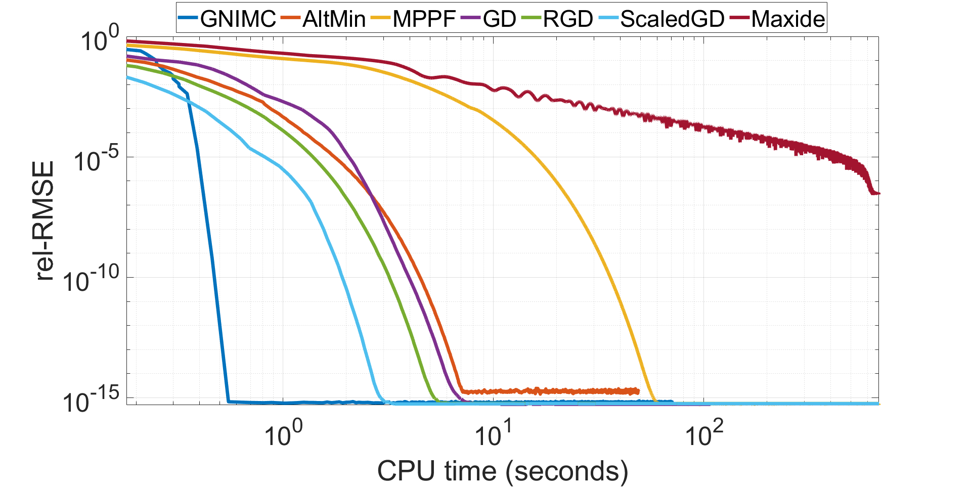
(a)

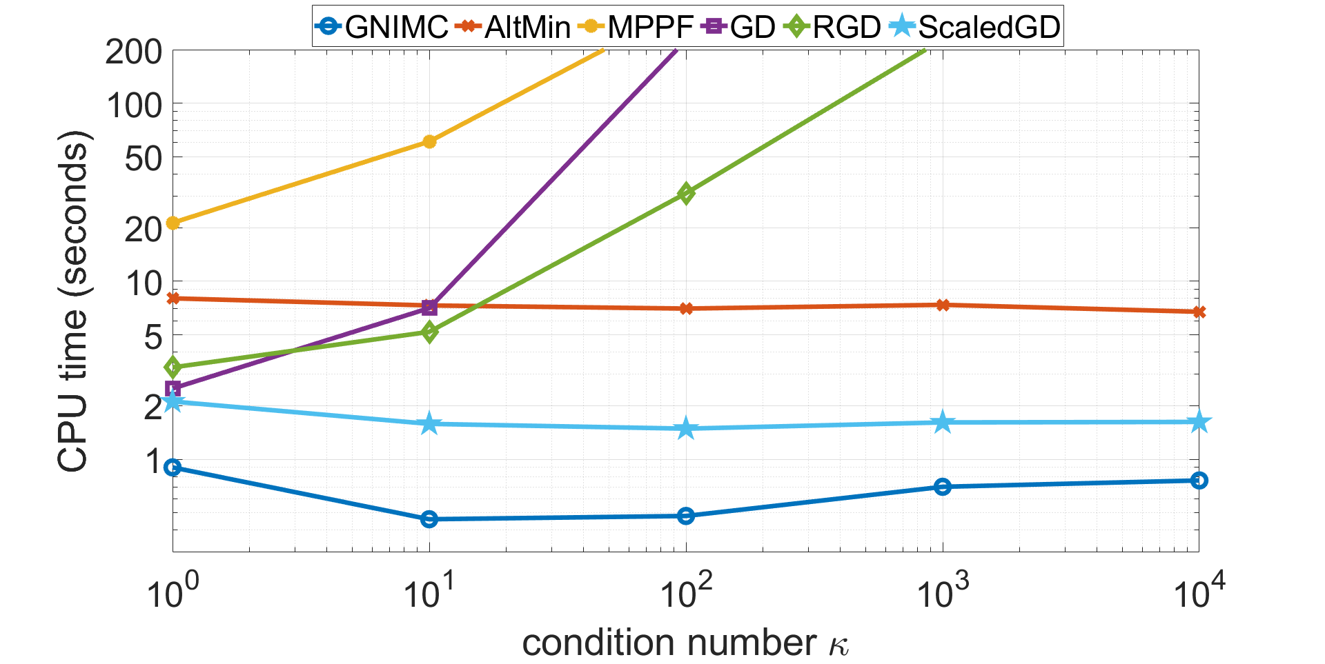
(b)

Figure 1: Left panel: rel-RMSE (17) as a function of CPU runtime for several IMC algorithms. Here $X^{*}$ has a condition number $\kappa=10$. Right panel: runtime till convergence as a function of $\kappa$, where each point corresponds to the median of $50$ independent realizations. In both panels, $X^{*}\in\mathbb{R}^{1000\times 1000}$, $A,B\in\mathbb{R}^{20\times 20}$, $r=10$ and oversampling ratio $\rho=1.5$.

We compare the performance of GNIMC to the following IMC algorithms, all implemented in MATLAB. AltMin [JD13]: our implementation of alternating minimization including the QR decomposition for reduced runtime; Maxide [XJZ13]: nuclear norm minimization as implemented by the authors; MPPF [ZDG18]: multi-phase Procrustes flow as implemented by the authors; GD, RGD: our implementations of vanilla gradient descent (GD) and a variant regularized by an imbalance factor $\|U^{\top}U-V^{\top}V\|_{F}$ (RGD); and ScaledGD [TMC21]: a preconditioned variant of gradient descent. Details on initialization, early stopping criteria and a tuning scheme for the hyperparameters of Maxide, MPPF, RGD and ScaledGD appear in Appendix G. GNIMC and AltMin require no tuning.

In each simulation we construct $U\in\mathbb{R}^{d_{1}\times r}$, $V\in\mathbb{R}^{d_{2}\times r}$, $A\in\mathbb{R}^{n_{1}\times d_{1}}$, $B\in\mathbb{R}^{n_{2}\times d_{2}}$ with entries i.i.d. from the standard normal distribution, and orthonormalize their columns. We then set $X^{*}=AUDV^{\top}B^{\top}$ where $D\in\mathbb{R}^{r\times r}$ is diagonal with entries linearly interpolated between $1$ and $\kappa$. A similar scheme was used in [ZDG18], with a key difference that we explicitly control the condition number of $X^{*}$ to study how it affects the performance of the various methods. Next, we sample $\Omega$ of a given size $|\Omega|$ from the uniform distribution over $[n_{1}]\times[n_{2}]$. Since $A$ and $B$ are known, the $n_{1}\times n_{2}$ matrix $X^{*}$ has only $(d_{1}+d_{2}-r)r$ degrees of freedom. Denote the oversampling ratio by $\rho=\frac{|\Omega|}{(d_{1}+d_{2}-r)r}$. As $\rho$ is closer to the information limit value of $1$, the more challenging the problem becomes. Notably, our simulations cover a broad range of settings, including much fewer observed entries and higher condition numbers than previous studies [XJZ13, ZDG18].

We measure the quality of an estimate $\hat{X}$ by its relative RMSE,

$$\texttt{rel-RMSE}=\frac{\|X^{*}-\hat{X}\|_{F}}{\|X^{*}\|_{F}}.$$ (17)

First, we explore the convergence rate of the various algorithms, by comparing their relative RMSE as a function of runtime, in the setting $n_{1}=n_{2}=1000$, $d_{1}=d_{2}=20$, $r=\kappa=10$ and $\rho=1.5$ (sampling rate $p=0.045\%$). Representative results of a single instance of the simulation, illustrating the behavior of the algorithms near convergence, are depicted in Fig. 1(left). As shown in the figure, GNIMC converges much faster than the competing algorithms due to its quadratic convergence rate.

Next, we examine how the runtime of each algorithm is affected by the number of observations and by the condition number. The runtime is defined as the CPU time required for the algorithm to (i) converge, namely satisfy one of the stopping criteria (detailed in Appendix G), and (ii) achieve $\texttt{rel-RMSE}\leq 10^{-4}$. If the runtime exceeds $20$ minutes without convergence, the run is stopped.

Figures 1(right) and 2(left) show the median recovery time on a log scale as a function of the condition number and of the oversampling ratio, respectively, in the same setting as above. Figure 2(right) corresponds to a larger matrix with $n_{1}=20000$, $n_{2}=1000$, $d_{1}=100$, $d_{2}=50$, $r=5$ and $\kappa=10$. Evidently, under a broad range of conditions, GNIMC is faster than the competing methods, in some cases by an order of magnitude. In general, the advantage of GNIMC with respect to the competing methods is more significant at low oversampling ratios.

Remarkably, the runtime of GNIMC, AltMin and ScaledGD shows almost no sensitivity to the condition number, as illustrated in Fig. 1(right). For GNIMC, this empirical observation is in agreement with Proposition 5.2, which states that the computational complexity of GNIMC does not depend on the condition number. In contrast, the runtime of the non-preconditioned gradient descent methods increases approximately linearly with the condition number.

Additional simulation results, including demonstration of the stability of GNIMC to noise, appear in Appendix H.

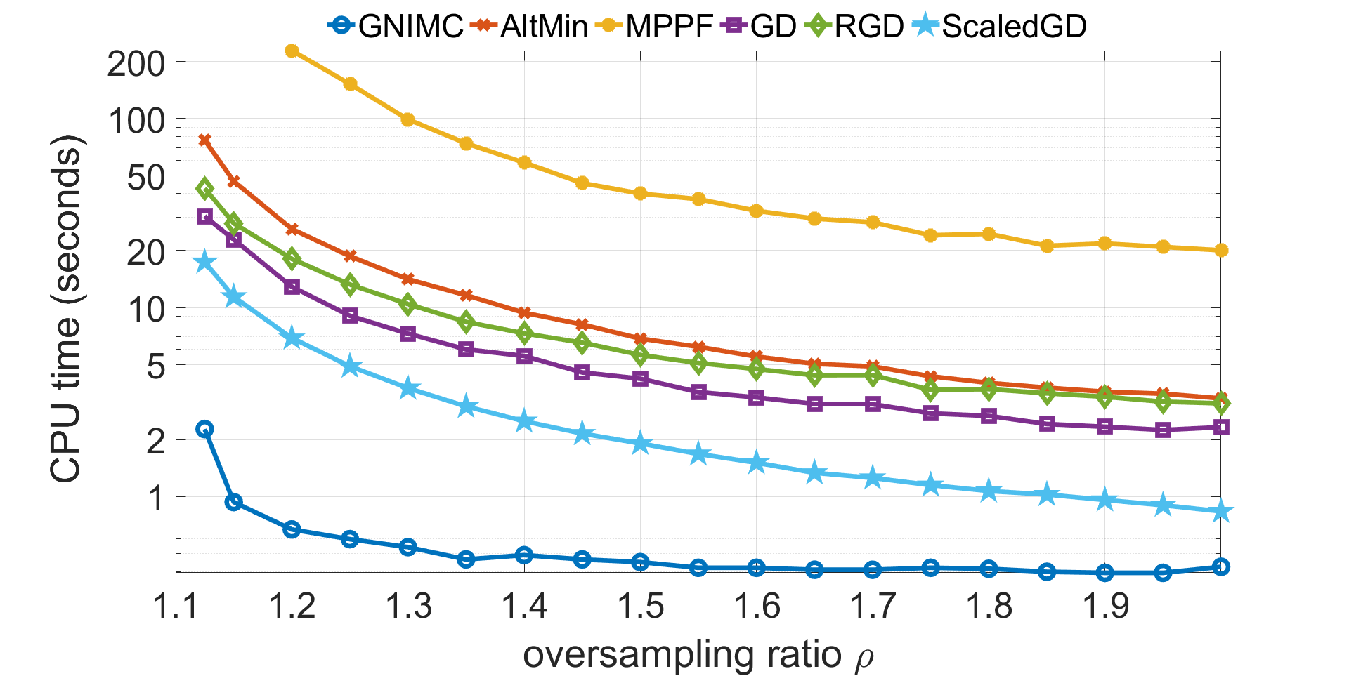
(a)

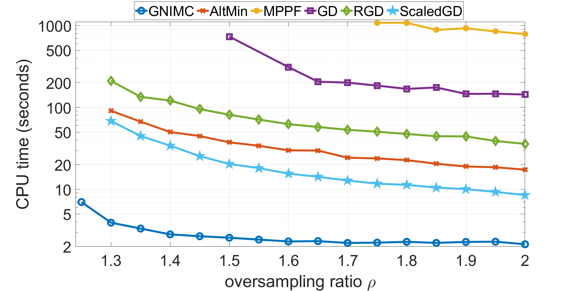
(b)

Figure 2: CPU runtime till convergence as a function of the oversampling ratio for several IMC algorithms. Left panel: $n_{1}=n_{2}=1000$, $d_{1}=d_{2}=20$ and $r=10$. Right panel: $n_{1}=20000$, $n_{2}=1000$, $d_{1}=100$, $d_{2}=50$ and $r=5$. In both panels $\kappa=10$. Each point corresponds to the median of $50$ independent realizations.

6.1 Demonstration of the rank estimation scheme

In this subsection we demonstrate the accuracy of our proposed rank estimation scheme (5). Figure 3 compares the estimated singular gaps $\hat{g}_{i}$ with the true ones $g_{i}$ for a matrix of approximate rank $r=5$ and only $p=0.1\%$ observed entries. We tested two values of $D$: $D=0$ and $D=(\sqrt{d_{1}d_{2}}/|\Omega|)^{1/2}$. The qualitative behavior depicted in the figure did not change in 50 independent realizations of the simulation. In particular, the estimated rank $\hat{r}=\max_{i}\hat{g}_{i}$ was always $5$ for both values of $D$.

The figure also demonstrates the trade-off in the choice of the value of $D$: for larger $D$, $\hat{g}_{i}$ is a more accurate estimate of $g_{i}$, but it also distorts the exact singular gaps $\sigma_{i}^{*}/\sigma^{*}_{i+1}$, especially at their tail (large values of $i$). Hence, in general, nonzero $D$ is suitable in case the rank of $X^{*}$ is expected to be relatively low compared to $d_{1},d_{2}$.

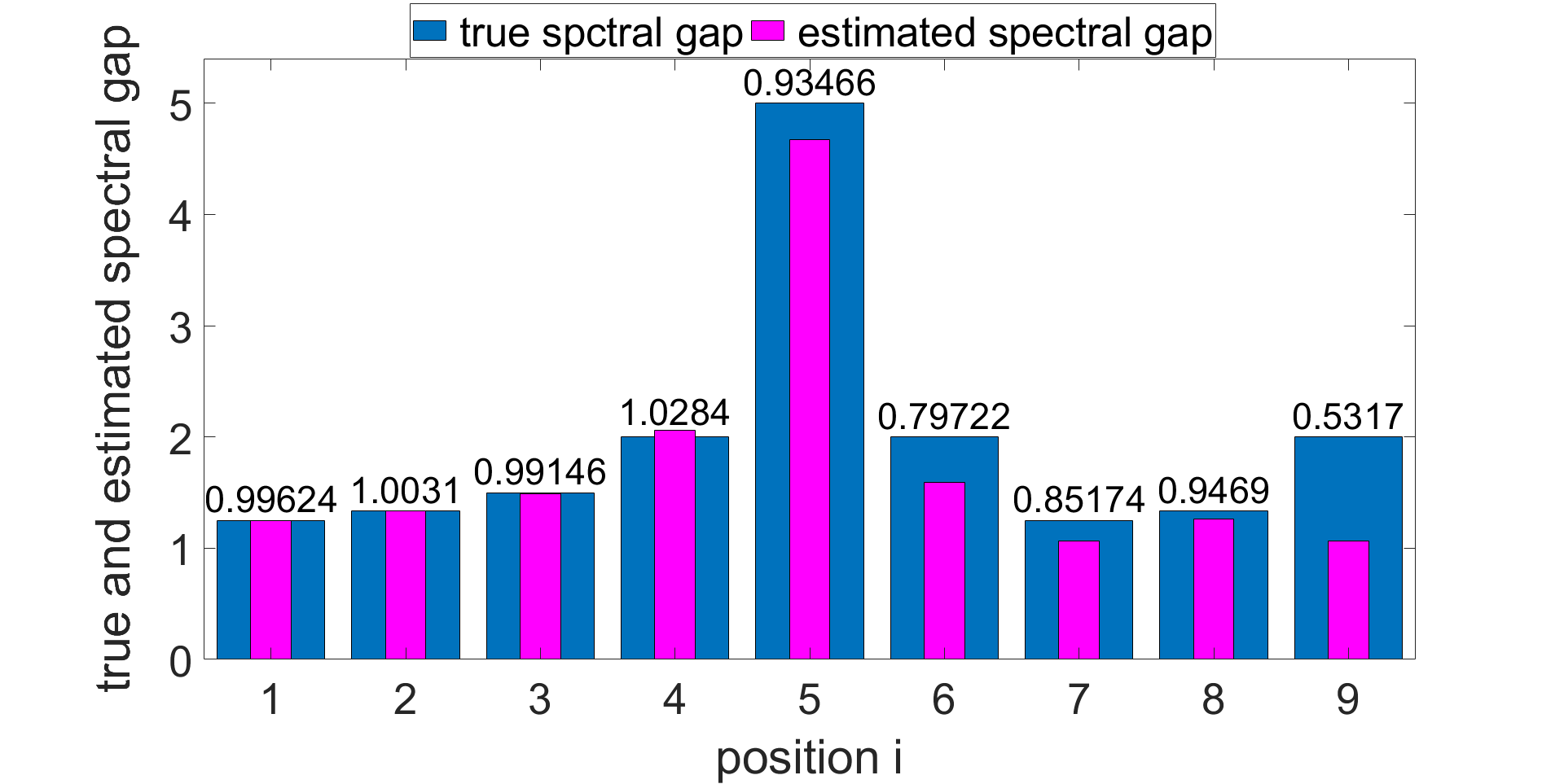
(a)

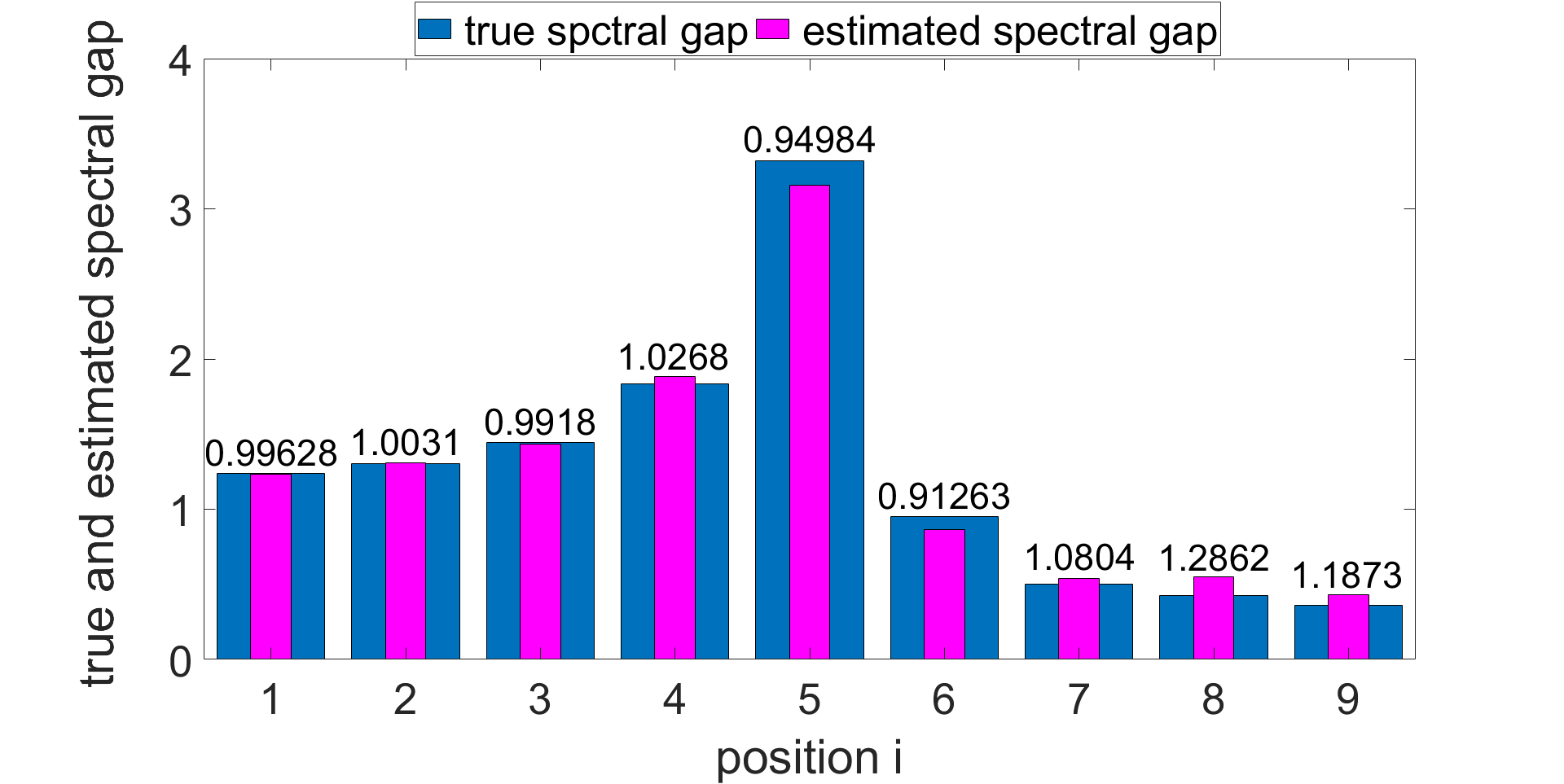
(b)

Figure 3: The estimated spectral gaps $\hat{g}_{i}$ (inner magenta) compared to the true ones $g_{i}$ (outer blue) as defined in (5), for $X^{*}\in\mathbb{R}^{30000\times 10000}$ of approximate rank $r=5$ with singular values $[5,4,3,2,1,0.2,0.1,0.08,0.06,0.03]$, side information $d_{1}=30$, $d_{2}=20$, and sampling rate $p=0.1\%$. The numbers above the bars indicate the ratio $\hat{g}_{i}/g_{i}$. Left panel: $D=0$. Right panel: $D=(\sqrt{d_{1}d_{2}}/|\Omega|)^{1/2}\approx 0.009$.

7 Summary and Discussion

In this work, we presented three contributions to the IMC problem: benign optimization landscape guarantee; provable rank estimation scheme; and a simple Gauss-Newton based method, GNIMC, to solve the IMC problem. We derived recovery guarantees for GNIMC, and showed empirically that it is faster than several competing algorithms. A key theoretical contribution is a proof that under relatively mild conditions, IMC satisfies an RIP, similar to the matrix sensing problem.

Interestingly, in our simulations GNIMC recovers the matrix significantly faster than first-order methods, including a very recent one due to [TMC21]. A possible explanation is that GNIMC makes large non-local updates, yet with the same time complexity as a single local gradient descent step. This raises the following intriguing questions: are there other non-convex problems for which non-local methods are faster than first-order ones? In particular, can these ideas be extended to faster training of deep neural networks?

Another interesting direction is extending our method to generalized frameworks of IMC. Important examples include recovering an unknown low rank $X^{*}$ which lies in some known linear subspace instead of property (1) [JM18], and non-linear IMC [ZSJD19].

Additional notation. In the following appendices, the Frobenius inner product between two matrices is denoted by $\braket{X,Y}=\operatorname{Tr}(Y^{\top}X)$, where $\operatorname{Tr}$ denotes the matrix trace. The adjoint of an operator $\mathcal{P}$ is denoted by $\mathcal{P}^{*}$. The spectral norm of an operator $\mathcal{P}$ that acts on matrices is defined as $\mathcal{\|}\mathcal{P}\|=\max_{X}\|\mathcal{P}(X)\|_{F}/\|X\|_{F}$.

Appendix A Proof of Theorem 3.3 (RIP for IMC)

In the following subsection we state and prove a novel RIP guarantee that is key to the connection between IMC and matrix sensing. Then, in the next subsection, we use this result to prove Theorem 3.3.

A.1 An auxiliary lemma

To present our RIP result in the context of IMC, recall the definition of the linear operator $\mathcal{P}_{AB}:\mathbb{R}^{n_{1}\times n_{2}}\to\mathbb{R}^{n_{1}\times n_{2}}$ which projects a matrix $X$ into the row and column spaces of the isometry matrices $A$ and $B$, respectively,

$$\mathcal{P}_{AB}(X)=AA^{\top}XBB^{\top}.$$ (18)

Note that since $\mathcal{P}_{AB}$ is a projection operator, $\|\mathcal{P}_{AB}\|=1$.

Lemma A.1.

Let $A\in\mathbb{R}^{n_{1}\times d_{1}}$ and $B\in\mathbb{R}^{n_{2}\times d_{2}}$ be two isometry matrices such that $\|A\|_{2,\infty}\leq\sqrt{\mu d_{1}/n_{1}}$ and $\|B\|_{2,\infty}\leq\sqrt{\mu d_{2}/n_{2}}$. Let $\delta\in[0,1)$, and assume $\Omega\subseteq[n_{1}]\times[n_{2}]$ is uniformly sampled with $|\Omega|\equiv n_{1}n_{2}p\geq(8/\delta^{2})\mu^{2}d_{1}d_{2}\log n$ where $n=\max\{n_{1},n_{2}\}$. Then w.p. at least $1-2n^{-2}$,

$$\|\tfrac{1}{p}\mathcal{P}_{AB}\mathcal{P}_{\Omega}\mathcal{P}_{AB}-\mathcal{P}_{AB}\|\leq\delta.$$ (19)

The numerical factor $8$ in the bound on the sample complexity $|\Omega|$ of Lemma A.1 can be replaced by any other scalar $\beta$ strictly greater than $8/3$, resulting in a modified probability guarantee $1-2n^{1-3\beta/8}$. We remark that $8/3$ is strict for our proof technique, which builds upon Recht’s work [Rec11], but can be improved by a more careful analysis, see the discussion after Proposition 5 in [Rec11].

The proof of Lemma A.1 uses the following matrix Bernstein inequality [Tro12, Theorem 1.6].

Lemma A.2.

Consider a finite set $\{Z_{k}\}$ of independent, random matrices with dimensions $n_{1}\times n_{2}$. Assume that each random matrix satisfies

$$\mathbb{E}[Z_{k}]=0\quad\mbox{and}\quad\|Z_{k}\|\leq R\quad\mbox{almost surely}.$$ (20)

Define $\sigma^{2}=\max\{\|\sum_{k}\mathbb{E}[Z_{k}Z_{k}^{\top}]\|,\|\sum_{k}\mathbb{E}[Z_{k}^{\top}Z_{k}]\|\}$. Then, for all $t\geq 0$,

$$\mathbb{P}\left[\left\|\sum_{k}Z_{k}\right\|\geq t\right]\leq(n_{1}+n_{2})\exp\left(-\frac{t^{2}/2}{\sigma^{2}+Rt/3}\right).$$ (21)

Proof of Lemma A.1.

The lemma assumes that $\Omega$ is uniformly sampled from the set of all collections of $m\equiv n_{1}n_{2}p$ entries of $[n_{1}]\times[n_{2}]$. Following [Rec11], in the following proof we assume instead a different probabilistic model: sampling with replacement. Let $\Omega^{\prime}=\{(i_{k},j_{k})\}_{k=1}^{m}$ be a collection of $m$ elements, each i.i.d. from the uniform distribution over $[n_{1}]\times[n_{2}]$. Define also the corresponding operator

$$\mathcal{R}_{\Omega^{\prime}}(X)=\sum_{k=1}^{m}\braket{e_{i_{k}}e_{j_{k}}^{\top},X}e_{i_{k}}e_{j_{k}}^{\top}.$$ (22)

In contrast to $\mathcal{P}_{\Omega}$, the operator $\mathcal{R}_{\Omega^{\prime}}$ is in general not a projection operator, since a pair of indices $(i,j)$ may have been sampled more than once. In the following, rather than (19), we prove the following modified inequality that involves $\mathcal{R}_{\Omega^{\prime}}$ in place of $\mathcal{P}_{\Omega}$,

$$\tfrac{1}{p}\|\mathcal{P}_{AB}\mathcal{R}_{\Omega^{\prime}}\mathcal{P}_{AB}-p\mathcal{P}_{AB}\|\leq\delta.$$ (23)

This inequality implies the original (19), as $\mathcal{R}_{\Omega^{\prime}}(X)$ reveals in general less information on $X$ than $\mathcal{P}_{\Omega}(X)$ does due to possible duplicates in $\Omega^{\prime}$; see the proof of Proposition 3 in [Rec11] for a rigorous formulation of this argument.

Since the elements of $\Omega^{\prime}$ are uniformly sampled from the set $[n_{1}]\times[n_{2}]$ and $|\Omega^{\prime}|=m\equiv pn_{1}n_{2}$, the expectation value of $\mathcal{R}_{\Omega^{\prime}}$ over the random set $\Omega^{\prime}$ is $p$ times the identity operator. Hence,

$$\mathbb{E}[\mathcal{P}_{AB}\mathcal{R}_{\Omega^{\prime}}\mathcal{P}_{AB}]=\mathcal{P}_{AB}\mathbb{E}[\mathcal{R}_{\Omega^{\prime}}]\mathcal{P}_{AB}=p\mathcal{P}_{AB}^{2}=p\mathcal{P}_{AB},$$ (24)

where $\mathcal{P}_{AB}$ is defined in (18). We thus conclude that (23) is simply a concentration inequality, which we shall prove using Lemma A.2.

Let $X\in\mathbb{R}^{n_{1}\times n_{2}}$, and decompose it as $X=\sum_{i,j}\braket{X,e_{i}e_{j}^{\top}}e_{i}e_{j}^{\top}$. For future use, we define the linear operator $\mathcal{T}_{ij}:\mathbb{R}^{n_{1}\times n_{2}}\to\mathbb{R}^{n_{1}\times n_{2}}$ as

$$\mathcal{T}_{ij}(X)=\braket{X,\mathcal{P}_{AB}(e_{i}e_{j}^{\top})}\mathcal{P}_{AB}(e_{i}e_{j}^{\top})=\braket{\mathcal{P}_{AB}(X),e_{i}e_{j}^{\top}}\mathcal{P}_{AB}(e_{i}e_{j}^{\top}),$$ (25)

and present some related equalities. By standard properties of the trace operator,

$$\mathcal{P}_{AB}\mathcal{R}_{\Omega^{\prime}}\mathcal{P}_{AB}=\sum_{k=1}^{m}\mathcal{T}_{i_{k}j_{k}}.$$ (26)

Hence, taking the expectation over $(i,j)$ uniformly sampled from $[n_{1}]\times[n_{2}]$ gives that

$$\mathbb{E}[\mathcal{T}_{ij}] =\frac{1}{m}\mathbb{E}\left[\sum_{k=1}^{m}\mathcal{T}_{i_{k}j_{k}}\right]=\frac{1}{pn_{1}n_{2}}\mathbb{E}[\mathcal{P}_{AB}\mathcal{R}_{\Omega^{\prime}}\mathcal{P}_{AB}]=\frac{1}{n_{1}n_{2}}\mathcal{P}_{AB}.$$ (27)

In addition, by the definition (25) of $\mathcal{T}_{ij}$ and the fact that $\mathcal{P}_{AB}$ is a projection,

$$\mathcal{P}_{AB}\mathcal{T}_{ij}=\mathcal{T}_{ij}\mathcal{P}_{AB}=\mathcal{T}_{ij}.$$ (28)

Finally, by inserting (26) into inequality (23), we obtain that our goal is to bound $\|\sum_{k=1}^{m}\mathcal{T}_{i_{k}j_{k}}-p\mathcal{P}_{AB}\|=\|\sum_{k=1}^{m}\mathcal{D}_{i_{k}j_{k}}\|$, where the operator $\mathcal{D}_{ij}:\mathbb{R}^{n_{1}\times n_{2}}\to\mathbb{R}^{n_{1}\times n_{2}}$ is given by

$$\mathcal{D}_{ij}=\mathcal{T}_{ij}-\frac{p}{m}\mathcal{P}_{AB}=\mathcal{T}_{ij}-\frac{1}{n_{1}n_{2}}\mathcal{P}_{AB}.$$

By (27), $\mathbb{E}[\mathcal{D}_{ij}]=0$. To employ Lemma A.2 to the set $\{\mathcal{D}_{i_{k},j_{k}}\}_{k=1}^{m}$, we first need to (i) find a scalar $R$ such that $\|\mathcal{D}_{ij}\|\leq R$ almost surely, and (ii) bound $\max\{\|\sum_{k=1}^{m}\mathbb{E}[\mathcal{D}_{i_{k}j_{k}}\mathcal{D}_{i_{k}j_{k}}^{*}]\|,$ $\|\sum_{k=1}^{m}\mathbb{E}[\mathcal{D}_{i_{k}j_{k}}^{*}\mathcal{D}_{i_{k}j_{k}}]\|\}=\|\sum_{k=1}^{m}\mathbb{E}[\mathcal{D}_{i_{k}j_{k}}^{2}]\|$, where the equality follows since $\mathcal{D}_{ij}$ is self-adjoint w.r.t. the Frobenius inner product.

We begin with bounding $\|\mathcal{D}_{ij}\|\equiv\max_{X}\|\mathcal{D}_{ij}(X)\|_{F}/\|X\|_{F}$. Recall that if $X$ and $Y$ are positive semidefinite matrices, then $\|X-Y\|_{2}\leq\max\{\|X\|_{2},\|Y\|_{2}\}$. Since any operator can be represented by a matrix, a similar result holds for operators with the spectral norm. As both $\mathcal{T}_{ij}$ and $\mathcal{P}_{AB}$ are positive semidefinite and $\mathcal{P}_{AB}$ is a projection, we have

$$\|\mathcal{D}_{ij}\|\leq\max\{\|\mathcal{T}_{ij}\|,\frac{1}{n_{1}n_{2}}\|\mathcal{P}_{AB}\|\}=\max\{\|\mathcal{T}_{ij}\|,\frac{1}{n_{1}n_{2}}\}.$$ (29)

Let us bound $\|\mathcal{T}_{ij}\|$. By the Cauchy-Schwarz inequality,

$$\|\mathcal{T}_{ij}(X)\| =|\braket{X,\mathcal{P}_{AB}(e_{i}e_{j}^{\top})}|\cdot\|\mathcal{P}_{AB}(e_{i}e_{j}^{\top})\|_{F}\leq\|\mathcal{P}_{AB}(e_{i}e_{j}^{\top})\|_{F}^{2}\|X\|_{F}.$$

Inserting the definition of $\mathcal{P}_{AB}$ (18), the spectral norm of $\mathcal{T}_{ij}$ is bounded as

$$\|\mathcal{T}_{ij}\| \leq\|\mathcal{P}_{AB}(e_{i}e_{j}^{\top})\|_{F}^{2}=\|AA^{\top}e_{i}e_{j}^{\top}BB^{\top}\|_{F}^{2}\stackrel{{\scriptstyle(a)}}{{\leq}}\|AA^{\top}e_{i}\|^{2}\|BB^{\top}e_{j}\|^{2}$$

$$\stackrel{{\scriptstyle(b)}}{{=}}\|A^{\top}e_{i}\|^{2}\|B^{\top}e_{j}\|^{2}\leq\|A\|^{2}_{2,\infty}\|B\|^{2}_{2,\infty}\stackrel{{\scriptstyle(c)}}{{\leq}}\frac{\mu^{2}d_{1}d_{2}}{n_{1}n_{2}},$$ (30)

where (a) follows from the Cauchy-Schwarz inequality, (b) from the isometry assumption, and (c) from the assumed bound on the row norms of $A$ and $B$. Plugging (A.1) into (29) yields

$$\|\mathcal{D}_{ij}\|\leq\max\{\frac{\mu^{2}d_{1}d_{2}}{n_{1}n_{2}},\frac{1}{n_{1}n_{2}}\}=\frac{\mu^{2}d_{1}d_{2}}{n_{1}n_{2}}\equiv R,$$ (31)

where the equality follows since $\mu\geq 1$ by the definition of incoherence (Definition 2.1). Next, we bound $\|\sum_{k=1}^{m}\mathbb{E}[\mathcal{D}_{i_{k}j_{k}}^{2}]\|$. Combining (28), (27) and the fact that both $\mathcal{T}_{ij}^{2}$ and $\mathcal{P}_{AB}$ are positive semidefinite yields

$$\|\mathbb{E}[\mathcal{D}_{ij}^{2}]\| =\|\mathbb{E}[\mathcal{T}_{ij}^{2}-\frac{2}{n_{1}n_{2}}\mathcal{T}_{ij}+\frac{1}{n_{1}^{2}n_{2}^{2}}\mathcal{P}_{AB}]\|=\|\mathbb{E}[\mathcal{T}_{ij}^{2}]-\frac{1}{n_{1}^{2}n_{2}^{2}}\mathcal{P}_{AB}\|$$

$$\leq\max\{\|\mathbb{E}[\mathcal{T}_{ij}^{2}]\|,\frac{1}{n_{1}^{2}n_{2}^{2}}\|\mathcal{P}_{AB}\|\}=\max\{\|\mathbb{E}[\mathcal{T}_{ij}^{2}]\|,\frac{1}{n_{1}^{2}n_{2}^{2}}\}.$$

Let us bound $\|\mathbb{E}[\mathcal{T}_{ij}^{2}]\|$. Since $\mathcal{T}_{ij}$ is positive semidefinite, we have $\mathcal{T}_{ij}^{2}\preccurlyeq\|\mathcal{T}_{ij}\|\mathcal{T}_{ij}$. Thus $\mathbb{E}[\mathcal{T}_{ij}^{2}]\preccurlyeq\mathbb{E}[\|\mathcal{T}_{ij}\|\mathcal{T}_{ij}]\preccurlyeq\frac{\mu^{2}d_{1}d_{2}}{n_{1}n_{2}}\mathbb{E}[\mathcal{T}_{ij}]$, where the last inequality follows from the deterministic bound (A.1). Together with (27) this implies

$$\|\mathbb{E}[\mathcal{T}_{ij}^{2}]\| \leq\frac{\mu^{2}d_{1}d_{2}}{n_{1}n_{2}}\|\mathbb{E}[\mathcal{T}_{ij}]\|=\frac{\mu^{2}d_{1}d_{2}}{n_{1}^{2}n_{2}^{2}}\|\mathcal{P}_{AB}\|=\frac{\mu^{2}d_{1}d_{2}}{n_{1}^{2}n_{2}^{2}}.$$

We thus obtain the bound

$$\|\sum_{k=1}^{m}\mathbb{E}[\mathcal{D}_{i_{k}j_{k}}^{2}]\|=m\cdot\|\mathbb{E}[\mathcal{D}_{ij}^{2}]\|\leq m\frac{\mu^{2}d_{1}d_{2}}{n_{1}^{2}n_{2}^{2}}=\frac{p\mu^{2}d_{1}d_{2}}{n_{1}n_{2}}\equiv\sigma^{2}.$$

Plugging this together with the bound $\|\mathcal{D}_{ij}\|\leq R$ in (31) into Lemma A.2 yields

$$\mathbb{P}\left[\left\|\sum_{k=1}^{m}\mathcal{D}_{i_{k}j_{k}}\right\|>p\delta\right] \leq(n_{1}+n_{2})\exp\left(-\frac{p^{2}\delta^{2}/2}{\frac{p\mu^{2}d_{1}d_{2}}{n_{1}n_{2}}+\frac{\mu^{2}d_{1}d_{2}}{n_{1}n_{2}}p\delta/3}\right)\leq 2n\exp\left(-\frac{3\delta^{2}m}{8\mu^{2}d_{1}d_{2}}\right).$$

Assuming that $m\geq(8/\delta^{2})\mu^{2}d_{1}d_{2}\log n$ gives

$$\mathbb{P}\left[\left\|\sum_{k=1}^{m}\mathcal{D}_{i_{k}j_{k}}\right\|>p\delta\right] \leq 2ne^{-3\log n}=2n^{-2}.$$

This completes the proof of (23), and thus of (19). ∎

A.2 Proof of Theorem 3.3

Let $M\in\mathbb{R}^{d_{1}\times d_{2}}$, and denote $X=AMB^{\top}$. By definition (3) of $\mathcal{A}$,

$$\frac{1}{p}\|\mathcal{P}_{\Omega}(X)\|_{F}^{2}=\frac{1}{p}\|\mathcal{P}_{\Omega}(AMB^{\top})\|_{F}^{2}=\|\mathcal{A}(M)\|^{2}.$$ (32)

Next, observe that $\mathcal{P}_{AB}(X)=AA^{\top}AMB^{\top}BB^{\top}=AMB^{\top}=X$. Hence

$$\|\mathcal{P}_{\Omega}(X)\|_{F}^{2} =\braket{\mathcal{P}_{\Omega}(X),\mathcal{P}_{\Omega}(X)}=\braket{X,\mathcal{P}_{\Omega}(X)}=\braket{X,pX}+\braket{X,\mathcal{P}_{\Omega}(X)-pX}$$

$$=p\|X\|_{F}^{2}+\braket{\mathcal{P}_{AB}(X),\mathcal{P}_{\Omega}\mathcal{P}_{AB}(X)-p\mathcal{P}_{AB}(X)}$$

$$=p\|X\|_{F}^{2}+\braket{X,\mathcal{P}_{AB}\mathcal{P}_{\Omega}\mathcal{P}_{AB}(X)-p\mathcal{P}_{AB}(X)}.$$

Applying the Cauchy-Schwarz inequality and (19) of Lemma A.1 yields

$$\left|\|\mathcal{P}_{\Omega}(X)\|_{F}^{2}-p\|X\|_{F}^{2}\right| =|\braket{X,\mathcal{P}_{AB}\mathcal{P}_{\Omega}\mathcal{P}_{AB}(X)-p\mathcal{P}_{AB}(X)}|$$

$$\leq\|X\|_{F}\|\mathcal{P}_{AB}\mathcal{P}_{\Omega}\mathcal{P}_{AB}(X)-p\mathcal{P}_{AB}(X)\|_{F}\leq p\delta\|X\|_{F}^{2}.$$

Hence

$$(1-\delta)\|X\|_{F}^{2}\leq\frac{1}{p}\|\mathcal{P}_{\Omega}(X)\|_{F}^{2}\leq(1+\delta)\|X\|_{F}^{2}.$$ (33)

Since $A,B$ are isometries, $\|X\|_{F}=\|AMB^{\top}\|_{F}=\|M\|_{F}$. Plugging this together with (32) into (33) yields the RIP (4). ∎

In the following remark, we extend the connection between IMC and matrix sensing (MS) to another setting of the two problems, where the goal is to find the minimal rank matrix that agrees with the observations.

Remark A.3.

An alternative setting of IMC, which does not assume a known rank but does assume noise-free observations, is to find a matrix with the lowest possible rank that is consistent with the data,

$$\min_{M}\text{ rank}(M)\quad\text{s.t. }\mathcal{P}_{\Omega}(AMB^{\top})=\mathcal{P}_{\Omega}(X^{*}).$$ (IMC*)

The analogous setting of MS is

$$\min_{M}\text{ rank}(M)\quad \text{s.t. }\mathcal{A}(M)=\mathcal{A}(M^{*}).$$ (MS*)

With the sensing operator $\mathcal{A}$ defined in (3), (IMC*) is in the form of (MS*). Since this sensing operator satisfies the RIP under certain conditions as guaranteed by Theorem 3.3, the connection between IMC and MS holds in this setting as well.

Appendix B Proof of Theorem 4.1 (Rank Estimation)

The proof of the theorem is based on the following lemma, which employs Lemma A.1 to bound the difference between the singular values of $X^{*}$ and those of $\hat{X}=\mathcal{P}_{AB}(Y)/p$.

Lemma B.1.

Let $X^{*}\in\mathbb{R}^{n_{1}\times n_{2}}$ be a matrix which satisfies (1) with $\mu$-incoherent matrices $A,B$. Let $\delta,\epsilon$ and $\Omega$ be defined as in Theorem 4.1 with constant $c<1/2$. Then w.p. at least $1-2n^{-2}$,

$$|\hat{\sigma}_{i}-\sigma_{i}^{*}|\leq 2c\delta,\quad\forall i,$$ (34)

where $\sigma_{i}^{*}=\sigma_{i}(X^{*})$.

Proof.

Since $X^{*}$ satisfies the side information property (1), we have $\mathcal{P}_{AB}(X^{*})=X^{*}$. Hence

$$\hat{X}=\frac{1}{p}\mathcal{P}_{AB}\mathcal{P}_{\Omega}(X^{*}+\mathcal{E})=\frac{1}{p}\mathcal{P}_{AB}\mathcal{P}_{\Omega}\mathcal{P}_{AB}(X^{*})+\frac{1}{p}\mathcal{P}_{AB}\mathcal{P}_{\Omega}(\mathcal{E}).$$

Using $\mathcal{P}_{AB}(X^{*})=X^{*}$ again, we get

$$\hat{X}-X^{*}=\left(\frac{1}{p}\mathcal{P}_{AB}\mathcal{P}_{\Omega}\mathcal{P}_{AB}-\mathcal{P}_{AB}\right)(X^{*})+\frac{1}{p}\mathcal{P}_{AB}\mathcal{P}_{\Omega}(\mathcal{E}).$$

Let $\delta^{\prime}=c\delta/\|X^{*}\|_{F}$. By definition, $\delta\leq\sigma_{2}^{*}+D\sigma_{1}^{*}<2\sigma_{1}^{*}$. Hence $\delta^{\prime}<1$ for $c<1/2$. Invoking Lemma A.1 with $|\Omega|\geq 8\mu^{2}d_{1}d_{1}\log(n)\|X^{*}\|_{F}^{2}/(c\delta)^{2}=8\mu^{2}d_{1}d_{1}\log(n)/{\delta^{\prime}}^{2}$ and using the condition $\epsilon\leq c\delta$ imply

$$\|\hat{X}-X^{*}\|_{F} \leq\left\|\left(\frac{1}{p}\mathcal{P}_{AB}\mathcal{P}_{\Omega}\mathcal{P}_{AB}-\mathcal{P}_{AB}\right)(X^{*})\right\|_{F}+\frac{1}{p}\|\mathcal{P}_{AB}\mathcal{P}_{\Omega}(\mathcal{E})\|_{F}\leq\delta^{\prime}\|X^{*}\|_{F}+\epsilon$$

$$\leq 2c\delta.$$ (35)

Hence also $\|\hat{X}-X^{*}\|_{F}\leq 2c\delta$. Equation 34 of the lemma follows by Weyl’s inequality. ∎

Proof of Theorem 4.1.

Denote $\hat{g}_{i}=g_{i}(\hat{X})$ and $g_{i}^{*}=g_{i}(X^{*})$. We need to show that $\operatorname*{arg\,max}_{i}\hat{g}_{i}=r$. Invoking Lemma B.1 implies

$$\hat{g}_{r} =\frac{\hat{\sigma}_{r}}{\hat{\sigma}_{r+1}+D\hat{\sigma}_{1}\sqrt{r}}\geq\frac{\sigma_{r}^{*}-2c\delta}{\sigma_{r}^{*}+2c\delta+D(\sigma_{1}^{*}+2c\delta)\sqrt{r}}.$$ (36)

By the definition of $\delta$, we have that $\delta\leq(1+D)\sigma_{1}^{*}<2\sigma_{1}^{*}$ and also $\delta\leq\sigma_{r}^{*}+D\sigma_{1}^{*}\sqrt{r}$. Plugging this into (36) yields

$$\hat{g}_{r} \geq\frac{\sigma_{r}^{*}-2c\delta}{\sigma_{r}^{*}+2c\delta+D(\sigma_{1}^{*}+4c\sigma_{1}^{*})\sqrt{r}}\geq\frac{\sigma_{r}^{*}-2c(\sigma_{r}^{*}+D\sigma_{1}^{*}\sqrt{r})}{(1+2c)(\sigma_{r}^{*}+D\sigma_{1}^{*}\sqrt{r})+4cD\sigma_{1}^{*}\sqrt{r}}$$

$$\geq\frac{\sigma_{r}^{*}-2c(\sigma_{r}^{*}+D\sigma_{1}^{*}\sqrt{r})}{(1+6c)(\sigma_{r}^{*}+D\sigma_{1}^{*}\sqrt{r})}=\frac{1}{1+6c}g_{r}^{*}-\frac{2c}{1+6c}.$$

Next, let $i\neq r$. Since $\delta\leq\sigma_{i+1}^{*}+D\sigma_{1}^{*}\sqrt{i}$, we similarly have

$$\hat{g}_{i} =\frac{\hat{\sigma}_{i}}{\hat{\sigma}_{i+1}+D\hat{\sigma}_{1}\sqrt{i}}\leq\frac{\sigma_{i}^{*}+2c\delta}{\sigma_{i+1}^{*}-2c\delta+D(\sigma_{1}^{*}-2c\delta)\sqrt{i}}\leq\frac{\sigma_{i}^{*}+2c(\sigma^{*}_{i+1}+D\sigma_{1}^{*}\sqrt{i})}{(1-2c)(\sigma_{i+1}^{*}+D\sigma_{1}^{*}\sqrt{i})-4cD\sigma^{*}_{i+1}\sqrt{i}}$$

$$\leq\frac{\sigma_{i}^{*}+2c(\sigma_{i}^{*}+D\sigma_{1}^{*}\sqrt{i})}{(1-6c)(\sigma_{i+1}^{*}D\sigma_{1}^{*}\sqrt{i})}=\frac{1}{1-6c}g_{i}^{*}+\frac{2c}{1-6c}.$$

By assumption, $g_{r}^{*}\geq\min\{(11/10)g_{i}^{*},1/10\}$. We thus obtain that $\hat{g}_{r}>\hat{g}_{i}$ for a sufficiently small constant $c$. Hence $\hat{r}=\operatorname*{arg\,max}_{i}\hat{g}_{i}=r$, as required. ∎

Appendix C Proof of Theorems 5.1, 5.4 and 3.1

Our proof of Theorem 3.1 follows by combining Theorem 3.3 with a general result due to [LLZ⁺20]. Consider the following general low rank optimization problem,

$$\min_{M\in\mathbb{R}^{d_{1}\times d_{2}}}f(M),\quad\text{s.t. rank}(M)\leq r.$$ (37)

By incorporating the rank constraint into the objective function, we obtain the factorized problem

$$\min_{U\in\mathbb{R}^{d_{1}\times r},V\in\mathbb{R}^{d_{2}\times r}}g(U,V)\equiv f(UV^{\top}).$$ (38)

The following result provides a sufficient condition on $f(M)$ such that $g(U,V)$ has no bad local minima. The condition is on the bilinear form of the Hessian of $f(M)$, defined as $\nabla^{2}f(M)[N,N]=\sum_{i,j,k,l}\frac{\partial^{2}f(M)}{\partial M_{ij}\partial M_{kl}}N_{ij}N_{kl}$.

Lemma C.1.

Let $\alpha,\beta$ be two positive constants that satisfy $\beta/\alpha\leq 3/2$. Assume that $f$ satisfies

$$\alpha\|N\|_{F}^{2}\leq\nabla^{2}f(M)[N,N]\leq\beta\|N\|_{F}^{2}$$ (39)

for all $M,N\in\mathbb{R}^{d_{1}\times d_{2}}$. If $f(M)$ has a critical point $M^{*}$ with $\text{rank}(M^{*})\leq r$, then any critical point $(U,V)$ of $g(U,V)$ in (38) is either a global minimum with $UV^{\top}=M^{*}$ or a strict saddle point.

Lemma C.1 is similar to Theorem III.1 in [LLZ⁺20], with one difference: in their Theorem III.1, it is sufficient that condition (39) holds only for matrices $M,N$ of rank at most $r_{1},r_{2}$, respectively, with $r_{1}=\min\{2r,d_{1},d_{2}\}$ and $r_{2}=\min\{4r,d_{1},d_{2}\}$. In fact, since [LLZ⁺20] assume $r\ll\min\{d_{1},d_{2}\}$ throughout their work, their Theorem III.1 is phrased with $r_{1}=2r$ and $r_{2}=4r$; however, it is straightforward to verify that in the general case, in which the rank of $M,N$ is bounded by $\min\{d_{1},d_{2}\}$, the theorem holds with $r_{1}=\min\{2r,d_{1},d_{2}\}$ and $r_{2}=\min\{4r,d_{1},d_{2}\}$. This condition is known as $(r_{1},r_{2})$-restricted strongly convex smoothness. Our condition is stronger, as it requires (39) to hold for all $M,N$, and thus implied by their Theorem III.1.

Proof of Theorem 3.1.

As discussed in the main text, the IMC problem can be written as a matrix sensing problem with the objective $f(M)=\|\mathcal{A}(M)-b\|^{2}$, the sensing operator $\mathcal{A}$ given in (3), and $b=\mathcal{A}(M^{*})+\text{Vec}_{\Omega}(\mathcal{E})/\sqrt{p}$. Furthermore, by Theorem 3.3, for the assumed $|\Omega|$, the operator $\mathcal{A}$ satisfies a $\min\{d_{1},d_{2}\}$-RIP (4) with a constant $\delta\leq 1/5$. Note that the $\min\{d_{1},d_{2}\}$-RIP of $\mathcal{A}:\mathbb{R}^{d_{1}\times d_{2}}\to\mathbb{R}^{d_{1}\times d_{2}}$ in fact means that (4) holds for any $d_{1}\times d_{2}$ matrix, since the rank of any such matrix is bounded by $\min\{d_{1},d_{2}\}$.

Next, for any $M,N\in\mathbb{R}^{d_{1}\times d_{2}}$, we have $\nabla f(M)=\mathcal{A}^{*}(\mathcal{A}(M)-b)$ and $\nabla^{2}f(M)[N,N]=\|\mathcal{A}(N)\|^{2}$ [ZLTW18, Section C.1]. Plugging the last equality into the RIP (4) of the sensing operator $\mathcal{A}$ yields

$$(1-\delta)\|N\|_{F}^{2}\leq\nabla^{2}f(M)[N,N]\leq(1+\delta)\|N\|_{F}^{2}.$$

Let $\alpha=1-\delta$ and $\beta=1+\delta$. Then $f$ satisfies Eq. 39 with the constants $\alpha,\beta$. Further, since $\delta\leq 1/5$, we have $\beta/\alpha\leq 3/2$. The corollary thus follows by Lemma C.1. ∎

Finally, the proof of Theorems 5.1 and 5.4 is straightforward thanks to our Theorem 3.3.

Proof of Theorems 5.1 and 5.4.

By Theorem 3.3, (IMC) is a special case of (MS) where the sensing operator $\mathcal{A}$ satisfies a rank $\min\{d_{1},d_{2}\}$-RIP with a constant $\delta\leq 1/2$. Theorems 5.1 and 5.4 thus follow from the MS recovery guarantees for GNMR [ZN22, Theorems 3.3-3.4]. ∎

Appendix D Computational Complexity Analysis

In Section 5 of the main text we briefly mentioned a way to use QR decompositions in order to efficiently find the minimal norm solution to the least squares problem (6). In the following subsection we describe the full procedure in detail. Then, in the next subsection, we prove Proposition 5.2 on the corresponding computational complexity. In both subsections we use the following simple result.

Lemma D.1.

Assume the conditions of Proposition 5.2. Then w.p. at least $1-2n^{-2}$, the factor matrices $U_{t},V_{t}$ of the iterates of GNIMC (Algorithm 1) have full column rank for all $t=0,1,...$.

Proof.

We prove that if

$$\|AU_{t}V_{t}^{\top}B^{\top}-X^{*}\|_{F}<\sigma_{r}^{*},$$ (40)

then $U_{t}$ and $V_{t}$ are full column rank. The lemma follows since (40) holds at $t=0$ by assumption (8a) with $c>1$, and at any $t>0$ w.p. at least $1-2n^{-2}$ by the contraction principle (9).

By combining Weyl’s inequality and (40),

$$|\sigma_{r}(AU_{t}V_{t}^{\top}B^{\top})-\sigma_{r}^{*}|\leq\|AU_{t}V_{t}^{\top}B^{\top}-X^{*}\|_{2}\leq\|AU_{t}V_{t}^{\top}B^{\top}-X^{*}\|_{F}<\sigma_{r}^{*}.$$

Since $A$ and $B$ are isometries, the above inequality implies that $|\sigma_{r}(U_{t}V_{t}^{\top})-\sigma_{r}^{*}|<\sigma_{r}^{*}$. Hence

$$0<\sigma_{r}(U_{t}V_{t}^{\top})\leq\min\{\sigma_{r}(U_{t})\|V_{t}\|_{2},\sigma_{r}(V_{t})\|U_{t}\|_{2}\},$$

which implies that both $\sigma_{r}(U_{t})$ and $\sigma_{r}(V_{t})$ are strictly positive, namely $U_{t},V_{t}$ have full column rank. ∎

D.1 A computationally efficient way to find the minimal norm solution to (6)

At iteration $t$ of GNIMC (Algorithm 1), our goal is to efficiently calculate the solution $(\Delta U_{t+1},\Delta V_{t+1})$ to the rank deficient least squares problem (6) whose norm $\|\Delta U_{t+1}\|_{F}^{2}+\|\Delta V_{t+1}\|_{F}^{2}$ is minimal. The least squares problem (6) at iteration $t$ reads

$$\operatorname*{arg\,min}_{\Delta U,\Delta V}\|\mathcal{P}_{\Omega}[A(U_{t}V_{t}^{\top}+U_{t}\Delta V^{\top}+\Delta UV_{t}^{\top})B^{\top}]-Y\|_{F}^{2}.$$ (41)

Denote the condition number of $X^{*}$ by $\kappa$. If $U_{t},V_{t}$ are approximately balanced and their product $U_{t}V_{t}^{\top}$ is close to $X^{*}$, their condition number scales as $\sqrt{\kappa}$. Hence, the condition number of the least squares problem (namely, the condition number of the operator defined in (44) below) scales as $\sqrt{\kappa}$. As a result, directly solving (41) leads to a factor of $\sqrt{\kappa}$ in the computational complexity. In the following, we describe a procedure that gives the same solution to (41) but eliminates the dependency in $\sqrt{\kappa}$, as proven in the next subsection. The procedure consists of two phases. First, we efficiently compute a feasible solution to (41), not necessarily the minimal norm one. Second, we describe how, given a solution to (41), we can efficiently compute the one with minimal norm, $(\Delta U_{t+1},\Delta V_{t+1})$. Algorithm 2 provides a sketch of this procedure.

By Lemma D.1, the factor matrices of the current iterate $U_{t},V_{t}$ are full column rank. Let $Q_{U}R_{U}$ and $Q_{V}R_{V}$ be the QR decompositions of $U_{t}$ and $V_{t}$, respectively, such that $Q_{U}\in\mathbb{R}^{d_{1}\times r}$ and $Q_{V}\in\mathbb{R}^{d_{2}\times r}$ are isometries, and $R_{U},R_{V}\in\mathbb{R}^{r\times r}$ are invertible. Instead of (41), we solve the following modified least squares problem,

$$(\Delta U^{\prime},\Delta V^{\prime}) =\operatorname*{arg\,min}_{\Delta U,\Delta V}\|\mathcal{P}_{\Omega}(AU_{t}V_{t}^{\top}B^{\top}+AQ_{U}\Delta V^{\top}B^{\top}+A\Delta UQ_{V}^{\top}B^{\top})-Y\|_{F}^{2}.$$ (42)

Here, $(\Delta U^{\prime},\Delta V^{\prime})$ is any feasible solution to (42), not necessarily the minimal norm one. Next, let

$$\Delta U^{\prime\prime}=\Delta U^{\prime}(R_{V}^{-1})^{\top}\quad\mbox{and}\quad\Delta V^{\prime\prime}=\Delta V^{\prime}(R_{U}^{-1})^{\top}.$$ (43)

It is easy to verify that $(\Delta U^{\prime\prime},\Delta V^{\prime\prime})$ is a feasible solution to the original least squares problem (41). This concludes the first part of the procedure, which can be viewed as preconditioning: as we show below, (42) has a lower condition number than (41), and it hence faster to solve by iterative methods. The reason for the better conditioning is that $Q_{U},Q_{V}$ both have condition number one rather than $\sqrt{\kappa}$. The detailed computational complexity analysis is deferred to the next subsection.

Next, we describe how to transform a feasible solution, such as $(\Delta U^{\prime\prime},\Delta V^{\prime\prime})$, into the minimal norm one $(\Delta U_{t+1},\Delta V_{t+1})$. To this end, we first express the least squares operator in terms of the sensing operator $\mathcal{A}$ defined in (3). In the matrix sensing formulation, the least squares problem (41) reads

$$\min_{(\Delta U,\Delta V)}\|\mathcal{P}_{\Omega}[A(U_{t}V_{t}^{\top}+U_{t}\Delta V^{\top}+\Delta UV_{t}^{\top})B^{\top}]-Y]\|_{F}$$

$$=\min_{(\Delta U,\Delta V)}\|\text{Vec}_{\Omega}[A(U_{t}V_{t}+U_{t}\Delta V^{\top}+\Delta UV_{t}^{\top})B^{\top}]/\sqrt{p}-\text{Vec}_{\Omega}(Y)/\sqrt{p}\|$$

$$=\min_{(\Delta U,\Delta V)}\|\mathcal{A}(U_{t}V_{t}^{\top}+U_{t}\Delta V^{\top}+\Delta UV_{t}^{\top})-b\|$$

$$=\min_{(\Delta U,\Delta V)}\|\mathcal{A}(U_{t}\Delta V^{\top}+\Delta UV_{t}^{\top})-b_{t}\|,$$

where $b=\text{Vec}_{\Omega}(Y)/\sqrt{p}$ and $b_{t}=b-\mathcal{A}(U_{t}V_{t}^{\top})$. The least squares operator $\mathcal{L}_{(U_{t},V_{t})}:\mathbb{R}^{(d_{1}+d_{2})\times r}\to\mathbb{R}^{m}$ is thus

$$\mathcal{L}_{(U_{t},V_{t})}\begin{pmatrix}U\\ V\end{pmatrix} =\mathcal{A}(U_{t}V^{\top}+UV_{t}^{\top}).$$ (44)

Let $\mathcal{K}=\ker\mathcal{L}_{(U_{t},V_{t})}$. By combining our RIP guarantee (Theorem 3.3) with the second part of Lemma 4.4 in [ZN22] which holds due to our Lemma D.1,

$$\mathcal{K}=\left\{\bigl{(}\begin{smallmatrix}U_{t}R\\ -V_{t}R^{\top}\end{smallmatrix}\bigr{)}\,\mid\,R\in\mathbb{R}^{r\times r}\right\}=\left\{\bigl{(}\begin{smallmatrix}Q_{U}R\\ -Q_{V}R^{\top}\end{smallmatrix}\bigr{)}\,\mid\,R\in\mathbb{R}^{r\times r}\right\}.$$ (45)

Also, $\text{dim}\{\mathcal{K}\}=r^{2}$ as $Q_{U},Q_{V}$ are isometries. By definition of the minimal norm solution $\bigl{(}\begin{smallmatrix}\Delta U_{t+1}\\ \Delta V_{t+1}\end{smallmatrix}\bigr{)}$, any other solution is of the form $\bigl{(}\begin{smallmatrix}\Delta U^{\prime\prime}\\ \Delta V^{\prime\prime}\end{smallmatrix}\bigr{)}=\bigl{(}\begin{smallmatrix}\Delta U_{t+1}\\ \Delta V_{t+1}\end{smallmatrix}\bigr{)}+\bigl{(}\begin{smallmatrix}K_{U}\\ K_{V}\end{smallmatrix}\bigr{)}$ where $\bigl{(}\begin{smallmatrix}\Delta U_{t+1}\\ \Delta V_{t+1}\end{smallmatrix}\bigr{)}\perp\mathcal{K}$ and $\bigl{(}\begin{smallmatrix}K_{U}\\ K_{V}\end{smallmatrix}\bigr{)}\in\mathcal{K}$. Hence, all we need to do is to subtract from $\bigl{(}\begin{smallmatrix}\Delta U^{\prime\prime}\\ \Delta V^{\prime\prime}\end{smallmatrix}\bigr{)}$ its component in $\mathcal{K}$. Denote the columns of $Q_{U},Q_{V}$ by $u_{i},v_{i}$ for $i\in[r]$, respectively, and let

$$K^{(ij)}=\frac{1}{\sqrt{2}}\begin{pmatrix}u_{i}e_{j}^{\top}\\ -v_{j}e_{i}^{\top}\end{pmatrix},\quad\forall(i,j)\in[r]\times[r].$$ (46)

Then the following set of $r^{2}$ matrices form an orthonormal basis for the kernel $\mathcal{K}$ of (45) under the Frobenius inner product $\braket{C,D}=\operatorname{Tr}(C^{\top}D)$:

$$\mathcal{K}_{B}=\left\{K^{(ij)}\,\mid\,(i,j)\in[r]\times[r]\right\}.$$ (47)

Let $\mathcal{I}$ be the identity operator. By calculating the projector $\mathcal{P}_{\mathcal{K}}$ onto the span of $\mathcal{K}_{B}$, we obtain the minimal norm solution $\bigl{(}\begin{smallmatrix}\Delta U_{t+1}\\ \Delta V_{t+1}\end{smallmatrix}\bigr{)}=(\mathcal{I}-\mathcal{P}_{\mathcal{K}})\bigl{(}\begin{smallmatrix}\Delta U^{\prime\prime}\\ \Delta V^{\prime\prime}\end{smallmatrix}\bigr{)}$.

The procedure described in this subsection is sketch in Algorithm 2.

input :  sampling operator $\mathcal{P}_{\Omega}$, observed matrix $Y$, side information matrices $(A,B)$, current iterate $(U_{t},V_{t})$

output : the minimal norm solution to (6)

$\triangleright$ Phase I: compute a feasible solution to (6)

1 compute $Q_{U}R_{U}$ and $Q_{V}R_{V}$, the QR decompositions of $U_{t}$ and $V_{t}$, respectively

2 compute $(\Delta U^{\prime},\Delta V^{\prime})$, any feasible solution to $\operatorname*{arg\,min}_{(\Delta U,\Delta V)}\|\mathcal{P}_{\Omega}[A(U_{t}V_{t}^{\top}+Q_{U}\Delta V^{\top}+\Delta UQ_{V}^{\top})B^{\top}]-Y\|_{F}^{2}$

3 set $\Delta U^{\prime\prime}=\Delta U^{\prime}(R_{V}^{-1})^{\top}$, $\Delta V^{\prime\prime}=\Delta V^{\prime}(R_{U}^{-1})^{\top}$

$\triangleright$ Phase II: compute the minimal norm solution to (6)

4 let $\mathcal{P}_{\mathcal{K}}:\mathbb{R}^{(d_{1}+d_{2})\times r}\to R^{(d_{1}+d_{2})\times r}$ be the projector onto $\mathcal{K}$, using its orthonormal basis given in (47)

5 set $\bigl{(}\begin{smallmatrix}\Delta U_{t+1}\\ \Delta V_{t+1}\end{smallmatrix}\bigr{)}=(\mathcal{I}-\mathcal{P}_{\mathcal{K}})\bigl{(}\begin{smallmatrix}\Delta U^{\prime\prime}\\ \Delta V^{\prime\prime}\end{smallmatrix}\bigr{)}$

return : $(\Delta U_{t+1},\Delta V_{t+1})$

Algorithm 2 Efficient procedure to compute the minimal norm solution to (6)

D.2 Proof of Proposition 5.2

For the analysis of the computational complexity of GNIMC with the minimal norm solution computed via Algorithm 2, we first prove the following auxiliary lemma. Recall that the condition number of an operator $\mathcal{P}:\mathbb{R}^{(d_{1}+d_{2})\times r}\to\mathbb{R}^{m}$ is defined as $\max_{Z}\{\|\mathcal{P}(Z)\|/\|Z\|_{F}\}/\min_{Z}\{\|\mathcal{P}(Z)\|/\|Z\|_{F}\}$.

Lemma D.2.

Let $\Omega,A,B$ be defined as in Proposition 5.2. Let $\mathcal{L}_{(Q_{U},Q_{V})}$ be the least squares operator of step 2 in Algorithm 2,

$$\mathcal{L}_{(Q_{U},Q_{V})}\begin{pmatrix}U\\ V\end{pmatrix} =\mathcal{A}(Q_{U}V^{\top}+UQ_{V}^{\top}).$$ (48)

Denote its condition number by $\kappa_{L}$. Then

$$\kappa_{L}\leq\sqrt{6}.$$ (49)

We remark that the bound in (49) can be slightly improved (up to $\kappa_{L}\leq\sqrt{2}$) at the cost of increasing $|\Omega|$.

Proof of Lemma D.2.

By combining assumption (7) and Theorem 3.3, the sensing operator $\mathcal{A}$ satisfies a $\min\{d_{1},d_{2}\}$-RIP with a constant $\delta\leq 1/2$. Hence, as in the proof of Lemma 4.2 in [ZN22], the minimal nonzero singular value of $\mathcal{L}_{(Q_{U},Q_{V})}$, $\sigma_{\text{min}}(\mathcal{L}_{(Q_{U},Q_{V})})$, is bounded from below by $\sqrt{1-\delta}\min\{\sigma_{r}(Q_{U}),\sigma_{r}(Q_{V})\}$ . Next, by Lemma D.1, $U_{t}$ and $V_{t}$ are of full column rank. Hence, $Q_{U}$ and $Q_{V}$ are isometries, and in particular $\sigma_{r}(Q_{U})=\sigma_{r}(Q_{V})=1$. We thus obtain $\sigma_{\text{min}}(\mathcal{L}_{(Q_{U},Q_{V})})\geq\sqrt{1-\delta}$.

We similarly bound from above the maximal singular value, $\sigma_{1}(\mathcal{L}_{(Q_{U},Q_{V})})$. Let $U\in\mathbb{R}^{d_{1}\times r}$, $V\in\mathbb{R}^{d_{2}\times r}$. Then

$$\left\|\mathcal{L}_{(Q_{U},Q_{V})}\begin{pmatrix}U\\ V\end{pmatrix}\right\|^{2} \stackrel{{\scriptstyle(a)}}{{\leq}}(1+\delta)\|UQ_{V}^{\top}+Q_{U}V^{\top}\|_{F}^{2}\stackrel{{\scriptstyle(b)}}{{\leq}}(1+\delta)(\|UQ_{V}^{\top}\|_{F}+\|Q_{U}V^{\top}\|_{F})^{2}$$

$$\stackrel{{\scriptstyle(c)}}{{=}}(1+\delta)(\|U\|_{F}^{2}+2\|U\|_{F}\|V\|_{F}+\|V\|_{F}^{2})\stackrel{{\scriptstyle(d)}}{{\leq}}2(1+\delta)(\|U\|_{F}^{2}+\|V\|_{F}^{2}),$$

where (a) follows by the RIP of $\mathcal{A}$, (b) by the triangle inequality, (c) by the fact that $Q_{U},Q_{V}$ are isometries, and (d) by $ab\leq(a^{2}+b^{2})/2$. Hence, the maximal singular value is bounded from above by $\sqrt{2(1+\delta)}$. The condition number of $\mathcal{L}_{(Q_{U},Q_{V})}$ is thus bounded as

$$\kappa_{L}\leq\sqrt{\frac{2(1+\delta)}{1-\delta}}\leq\sqrt{6}$$

where the second inequality follows since $\delta\leq 1/2$. ∎

We are now ready to prove Proposition 5.2.

Proof of Proposition 5.2.

According to our quadratic convergence guarantee, the number of GNIMC iterations till recovery with a fixed accuracy is constant. Thus, up to a multiplicative constant, the complexity of GNIMC is the same as the complexity of a single iteration, which we shall now analyze according to its sketch in Algorithm 2.

The complexity of step 2, which consists of QR factorizations of $d\times r$ matrices, is $\mathcal{O}(dr^{2})$ [GP03, Section 5.2.9]. Step 2 is separately analyzed below. Step 2 is dominated by the calculation of the matrix product, which costs $\mathcal{O}(dr^{2})$. Steps 2-2 are dominated by the calculation of the projection of a feasible solution $\bigl{(}\begin{smallmatrix}\Delta U^{\prime\prime}\\ \Delta V^{\prime\prime}\end{smallmatrix}\bigr{)}$ onto the kernel $\mathcal{K}$ given in (45). To this end, we first construct a matrix $K\in\mathbb{R}^{(d_{1}+d_{2})r\times r^{2}}$ whose columns are the vectorization of the elements of the orthonormal basis $\mathcal{K}_{B}$ given in (47). Then, to obtain the required projection, we calculate the product $KK^{\top}z$ where $z\equiv\text{Vec }\bigl{(}\begin{smallmatrix}\Delta U^{\prime\prime}\\ \Delta V^{\prime\prime}\end{smallmatrix}\bigr{)}\in\mathbb{R}^{(d_{1}+d_{2})r}$ is the vectorization of the feasible solution in hand. By first calculating $K^{\top}z$ and then $K(K^{\top}z)$ we obtain the complexity of $\mathcal{O}(dr^{3})$.

Finally, we analyze the complexity of step 2. GNIMC solves the least squares problem using the standard LSQR algorithm [PS82], which applies the conjugate gradient (CG) method to the normal equations. Each inner iteration of CG is dominated by the calculation of $AQ_{U}\Delta V^{\top}B^{\top}+A\Delta UQ_{V}^{\top}B^{\top}$ at the entries of $\Omega$ [PS82, Section 7.7]. To obtain a single entry of $AQ_{U}\Delta V^{\top}B^{\top}$, we calculate a single row of $AQ_{U}$, a single column of $\Delta V^{\top}B^{\top}$, and then take the product. Since $Q_{U}\in\mathbb{R}^{d_{1}\times r}$ and $\Delta V^{\top}\in\mathbb{R}^{r\times d_{2}}$, this sums up to $\mathcal{O}(d_{1}r+d_{2}r+r^{2})\sim\mathcal{O}(dr)$ operations. Similarly, calculating a single entry of $A\Delta UQ_{V}^{\top}B^{\top}$ takes $\mathcal{O}(dr)$ operations. The complexity of a single iteration of CG is thus $\mathcal{O}(dr|\Omega|)$.

Next, we analyze the required number of CG iterations. Let $\kappa_{L}$ be the condition number of the least squares operator $\mathcal{L}_{(Q_{U},Q_{V})}$ as defined in Lemma D.2. The residual error of CG decays at least linearly with a contraction factor $\frac{\kappa_{L}-1}{\kappa_{L}+1}$ [Hay18, Section 4]. By Lemma D.2, $\kappa_{L}$ is bounded by a constant, and hence the required number of CG iterations is also a constant. We thus conclude that the total complexity of step 2 is $\mathcal{O}(dr|\Omega|)$.

Putting everything together, the complexity of GNIMC is $\mathcal{O}(dr^{3}+dr|\Omega|)$. One of the conditions of the proposition is the lower bound $|\Omega|\geq 32\mu^{2}d_{1}d_{2}\log n$. W.l.o.g., we may assume $|\Omega|=32\mu^{2}d_{1}d_{2}\log n$ (if $|\Omega|$ is larger, we can ignore some of the observed entries). We thus obtain that the complexity of GNIMC is $\mathcal{O}(\mu^{2}dd_{1}d_{2}r\log n)$.

∎

D.3 Comparison to gradient descent

In this subsection we show that the per-iteration cost of GNIMC, as analyzed above, is of the same order as that of gradient descent. Denote $E_{\Omega}=\mathcal{P}_{\Omega}(AUV^{\top}B^{\top})-Y$, and let $f(U,V)=\|E_{\Omega}\|_{F}^{2}$ be the objective of the factorized matrix completion problem (2). Its gradient is

$$\nabla_{U}f(U,V) =2A^{\top}E_{\Omega}BV,\quad\nabla_{V}f(U,V)=2B^{\top}E_{\Omega}^{\top}AU.$$

As explained in the analysis of step 2 above, calculating $E_{\Omega}$ costs $\mathcal{O}(dr|\Omega|)$. Since $A^{\top}E_{\Omega}$ and $B^{\top}E_{\Omega}^{\top}$ have at most $r|\Omega|$ nonzero entries, this is also the cost of calculating $(A^{\top}E_{\Omega})B$ and $(B^{\top}E_{\Omega}^{\top})A$. Finally, calculating $(A^{\top}E_{\Omega}B)V$ and $(B^{\top}E_{\Omega}^{\top}A)U$ is $\mathcal{O}(d_{1}d_{2}r)$. The per-iteration complexity of gradient descent is thus $\mathcal{O}(dr|\Omega|+d_{1}d_{2}r)$. Under assumption (7) on $|\Omega|$, this coincides with the per-iteration complexity of GNIMC.

We remark that empirically, the overall complexity (namely, from initialization to convergence) of gradient descent seems so be much larger than that of GNIMC, see Section 6. This observation is in agreement with the theoretical analysis of gradient descent in [ZDG18], see their Theorem 5.5.

Appendix E Proof of Proposition 5.3 (Initialization Guarantee)

By its construction, $\bigl{(}\begin{smallmatrix}U_{0}\\ V_{0}\end{smallmatrix}\bigr{)}$ is perfectly balanced, $U_{0}^{\top}U_{0}=V_{0}^{\top}V_{0}$, and thus satisfies (8b). Hence, we only need to prove (8a). Let $\mathcal{A}$ be the sensing operator that corresponds to (IMC) as defined in (3). By Theorem 3.3, w.p. at least $1-2n^{-2}$, the operator $\mathcal{A}$ satisfies a $\min\{d_{1},d_{2}\}$-RIP with a constant $\delta=2/5$. Hence, according to Lemmas 5.1-5.2 in [TBS⁺16], or more explicitly Eq. (5.26) in their extended arXiv version, after $\tau\geq\log(c\sqrt{r}\kappa)/\log(1/(2\delta))\geq 5\log(c\sqrt{r}\kappa)$ iterations of (10) we have $\|M_{\tau}-M^{*}\|_{F}\leq\sigma_{r}^{*}/c$. Since $A,B$ are isometries, $\|AM_{\tau}B^{\top}-X^{*}\|_{F}=\|M_{\tau}-M^{*}\|_{F}\leq\sigma_{r}^{*}/c$. Hence $\bigl{(}\begin{smallmatrix}U_{0}\\ V_{0}\end{smallmatrix}\bigr{)}$ satisfies (8a) for any $\tau\geq 5\log(c\sqrt{r}\kappa)$. ∎

Appendix F Comparison to [GSG18]

[GSG18] derived results analogous to our Theorems 3.3 and 3.1. However, there are three main differences between the claims. First, the sample complexity for the RIP result in [GSG18] is

$$\mathcal{O}(\mu^{2}r\max\{d_{1},d_{2}\}\max\{d_{1}d_{2},\log^{2}n\}\log(1/\delta)/\delta^{2}),$$ (50)

compared to our $\mathcal{O}(\mu^{2}d_{1}d_{2}\log(n)/\delta^{2})$. We remark that in their notation, their claimed sample complexity is $\mathcal{O}(\mu^{2}\max\{d_{1},d_{2}\}\bar{r}^{2}r)$ where $\bar{r}=\max\{r,\log n\}$. However, there seems to be an error in their analysis. Their assumption is that $A/\sqrt{n_{1}}$ and $B/\sqrt{n_{2}}$ are isometries, and their corresponding incoherence assumption is $\|A\|_{2,\infty}^{2}\leq\mu\bar{r}$ and $\|B\|_{2,\infty}^{2}\leq\mu\bar{r}$ with a constant $\mu$ [GSG18, Assumption 1]. But since $A\in\mathbb{R}^{n_{1}\times d_{1}}$ and $B\in\mathbb{R}^{n_{2}\times d_{2}}$, either the assumption should be $\|A\|_{2,\infty}^{2}\leq\mu d_{1}$ and $\|B\|_{2,\infty}^{2}\leq\mu d_{2}$, or the parameter $\mu$ is not a constant but rather scales with $\max\{d_{1},d_{2}\}/\bar{r}$. In any case, in our notation their sample complexity is as given in (50).

Second, the RIP result in [GSG18] is for rank-$\min\{2r,d_{1},d_{2}\}$ matrices, compared to our stronger rank-$\min\{d_{1},d_{2}\}$ RIP. We remark that while their RIP result is formulated as $2r$-RIP, this implicitly assumes $r\ll\min\{d_{1},d_{2}\}$ (see also the discussion in Appendix C). In the general case, their guarantee is $\min\{2r,d_{1},d_{2}\}$-RIP.

Third, [GSG18] prove benign optimization landscape for the problem

$$\min_{U,V}\|\mathcal{P}_{\Omega}(AUV^{\top}B^{\top})-Y\|+\frac{1}{4}\|UU^{\top}-VV^{\top}\|_{F}^{2},$$ (51)

which is an imbalance regularized version of (2). Furthermore, it seems that their result cannot be readily extended to the vanilla IMC problem, as the regularization in (51) is essential in their proof.

Appendix G Additional Simulation Details

All algorithms are initialized with the same procedure, which is the spectral initialization, except for Maxide which is not factorization based and is by default initialized with the zero matrix.

Maxide gets as input a regularization parameter, and MPPF, GD, RGD and ScaledGD get a step size parameter. For each simulation setting, we tuned the optimal parameter out of $10$ logarithmically-scaled values. The permitted values for Maxide were $10^{-5},...,10^{-14}$, for MPPF, GD and RGD were $10^{-2}/\kappa,...,10^{\frac{1}{2}}/\kappa$ where $\kappa$ is the condition number of $X^{*}$, and for ScaledGD were $10^{-2},...,10^{\frac{1}{2}}$. In all simulations, we verified that the selected value is an interior point of the permitted set, so that it is close to optimal. We remark that the regularization coefficient of MPPF and RGD can also be tuned, but we observed it has a very little effect. For GNIMC, in all simulations we identically set the maximal number of iterations for the inner least-squares solver to $10$ if the observed error is low, $\frac{\|\mathcal{P}_{\Omega}(X_{t})-Y\|_{F}}{\|Y\|_{F}}\leq 10^{-4}$, and $1000$ otherwise. This scheme exhibits slightly better performance than setting a constant value of maximal inner iterations (but only marginally). While tuning this value for each simulation independently, as we did for the hyperparameters of the above algorithms, may enhance performance, we preferred to demonstrate the performance of a tuning-free version of GNIMC.

We used the following two stopping criteria for all methods: (i) small relative observed RMSE, $\frac{\|\mathcal{P}_{\Omega}(X_{t})-Y\|_{F}}{\|Y\|_{F}}\leq\epsilon$, or (ii) small relative estimate change $\frac{\|\mathcal{P}_{\Omega}(X_{t}-X_{t-1})\|_{F}}{\|\mathcal{P}_{\Omega}(X_{t})\|_{F}}\leq\epsilon$. In our simulations, we set $\epsilon=10^{-14}$. For a fair comparison, we disabled all the other early stopping criteria defined in the algorithms.

Appendix H Additional Simulation results

In subsection H.1 we demonstrate the stability of GNIMC to Gaussian noise. In subsection H.2 we demonstrate the insensitivity of several algorithms to the condition number of the underlying matrix in terms of the number of observations required for recovery.

H.1 Stability of GNIMC to noise

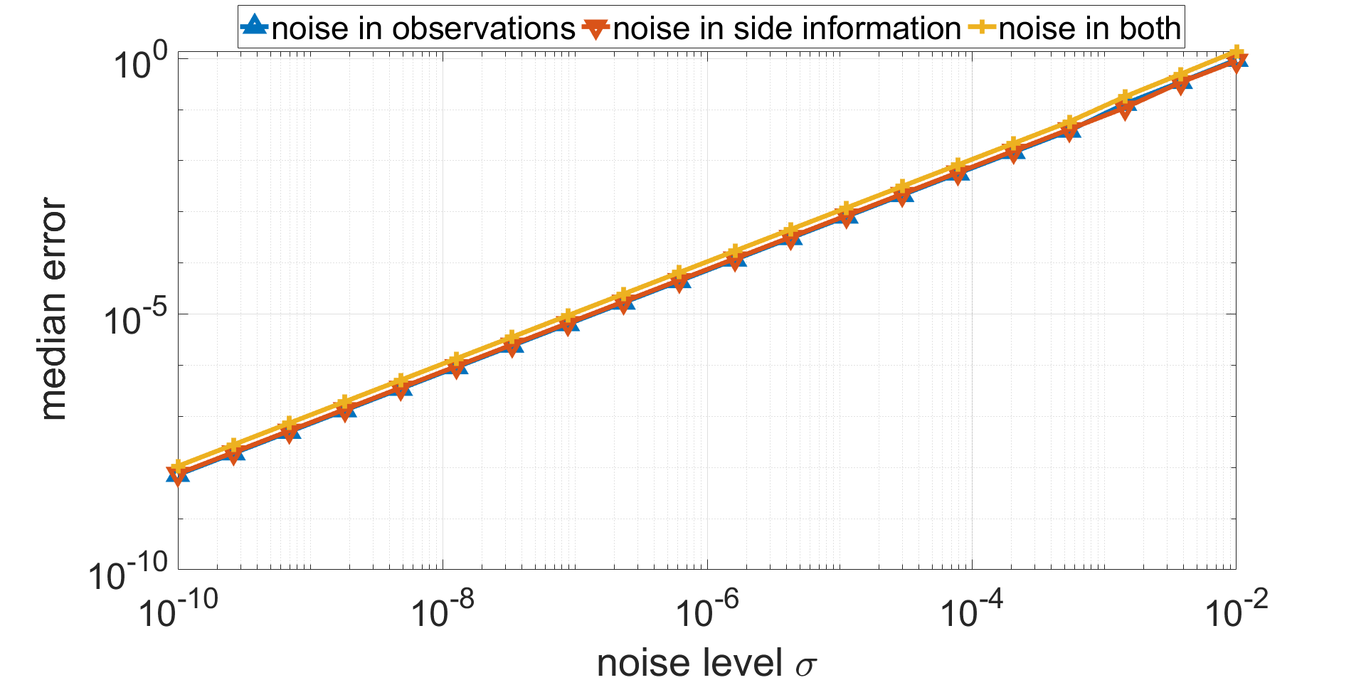
Figure 4: Stability of GNIMC to additive Gaussian noise, with the same settings as in Fig. 1(left).

Figure 4 demonstrates the stability of GNIMC to noise. In this simulation, either the observed entries $Y$, the side information matrices $A,B$, or both, are corrupted by additive Gaussian noise of zero mean and standard deviation $\sigma$. As seen in the figure, the error of GNIMC scales linearly with the noise level $\sigma$.

H.2 Insensitivity of several algorithms to the condition number

In Fig. 1(right) we addressed the sensitivity (or insensitivity) of several IMC algorithms to the condition number of $X^{*}$ in terms of their runtime. In this subsection, we explore another aspect of sensitivity to the condition number: rather than runtime, we study how the condition number affects the number of observations required for a successful recovery given no time constraints.

Table 2: Lowest oversampling ratio $\rho$ from which the median of rel-RMSE (17) is lower than $10^{-4}$, as a function of the condition number $\kappa$, in the setting $n_{1}=n_{2}=1000$, $d_{1}=d_{2}=20$, $r=10$. Each entry shows the median of $50$ independent realizations.

	$1$	$10$	$10^{2}$	$10^{3}$	$10^{4}$
GNIMC	$1.2$	$1.1$	$1.1$	$1.1$	$1.1$
AltMin	$1.1$	$1.1$	$1.1$	$1.1$	$1.1$
GD	$1.1$	$1.1$	$1.1$	$1.1$	$1.1$
RGD	$1.2$	$1.2$	$1.1$	$1.1$	$1.1$
ScaledGD	$1.2$	$1.1$	$1.2$	$1.2$	$1.1$
Maxide	$1.4$	$1.4$	$1.4$	$1.4$	$1.4$

In our simulations, we observed the following interesting phenomenon: For all algorithms, the number of observations $|\Omega|$ required for recovery is independent of the condition number $\kappa$. We demonstrate this in Table 2, which compares the minimal oversampling ratio, out of the values $\rho=1.1,1.2,...$, required by several algorithms to reach relative RMSE of $10^{-4}$. Since in this experiment our goal is to explore fundamental recovery abilities rather than speedy performance, the algorithms are given essentially unlimited runtime (in practice, the time limit was set to one CPU hour, and $3$ hours for GD and RGD in the case of $\kappa=10^{4}$). The table shows that the minimal oversampling ratio does not increase with $\kappa$; in fact, it sometimes slightly decreases when $\kappa$ is small. We did not include MPPF in Table 2 due to its long runtime; however, a limited set of simulations suggests that the same conclusion also holds for it.

Beyond illustrating the abilities of the algorithms, this result demonstrates a basic property of the IMC problem: insensitivity to the condition number. This result corresponds well with our RIP guarantee for IMC, Theorem 3.3, as the RIP holds for all matrices of certain ranks regardless of their condition number.

References

- [ABEV09] Jacob Abernethy, Francis Bach, Theodoros Evgeniou, and Jean-Philippe Vert. A new approach to collaborative filtering: Operator estimation with spectral regularization. Journal of Machine Learning Research, 10(Mar):803–826, 2009.
- [Can08] Emmanuel J Candes. The restricted isometry property and its implications for compressed sensing. Comptes rendus mathematique, 346(9-10):589–592, 2008.
- [CDH18] Kai-Yang Chiang, Inderjit S Dhillon, and Cho-Jui Hsieh. Using side information to reliably learn low-rank matrices from missing and corrupted observations. The Journal of Machine Learning Research, 19(1):3005–3039, 2018.
- [CR09] Emmanuel J Candès and Benjamin Recht. Exact matrix completion via convex optimization. Foundations of Computational mathematics, 9(6):717, 2009.
- [CWQ+18] Xing Chen, Lei Wang, Jia Qu, Na-Na Guan, and Jian-Qiang Li. Predicting miRNA–disease association based on inductive matrix completion. Bioinformatics, 34(24):4256–4265, 2018.
- [CZL+12] Tianqi Chen, Weinan Zhang, Qiuxia Lu, Kailong Chen, Zhao Zheng, and Yong Yu. Svdfeature: a toolkit for feature-based collaborative filtering. The Journal of Machine Learning Research, 13(1):3619–3622, 2012.
- [GP03] Gene Golub and Victor Pereyra. Separable nonlinear least squares: the variable projection method and its applications. Inverse problems, 19(2):R1, 2003.
- [GSG18] Mohsen Ghassemi, Anand Sarwate, and Naveen Goela. Global optimality in inductive matrix completion. In 2018 IEEE International Conference on Acoustics, Speech and Signal Processing (ICASSP), pages 2226–2230. IEEE, 2018.
- [Hay18] Ken Hayami. Convergence of the conjugate gradient method on singular systems. arXiv preprint arXiv:1809.00793, 2018.
- [JD13] Prateek Jain and Inderjit S Dhillon. Provable inductive matrix completion. arXiv preprint arXiv:1306.0626, 2013.
- [JM18] Pratik Jawanpuria and Bamdev Mishra. A unified framework for structured low-rank matrix learning. In International Conference on Machine Learning, pages 2254–2263. PMLR, 2018.
- [JNS13] Prateek Jain, Praneeth Netrapalli, and Sujay Sanghavi. Low-rank matrix completion using alternating minimization. In Proceedings of the forty-fifth annual ACM symposium on Theory of computing, pages 665–674. ACM, 2013.
- [KMO09] Raghunandan H Keshavan, Andrea Montanari, and Sewoong Oh. Low-rank matrix completion with noisy observations: a quantitative comparison. In 2009 47th Annual Allerton Conference on Communication, Control, and Computing (Allerton), pages 1216–1222. IEEE, 2009.
- [KMO10] Raghunandan H Keshavan, Andrea Montanari, and Sewoong Oh. Matrix completion from a few entries. IEEE transactions on Information Theory, 56(6):2980–2998, 2010.
- [LLZ+20] Shuang Li, Qiuwei Li, Zhihui Zhu, Gongguo Tang, and Michael B Wakin. The global geometry of centralized and distributed low-rank matrix recovery without regularization. IEEE Signal Processing Letters, 27:1400–1404, 2020.
- [LYL+18] Chengqian Lu, Mengyun Yang, Feng Luo, Fang-Xiang Wu, Min Li, Yi Pan, Yaohang Li, and Jianxin Wang. Prediction of lncRNA–disease associations based on inductive matrix completion. Bioinformatics, 34(19):3357–3364, 2018.
- [MCG+11] Aditya Krishna Menon, Krishna-Prasad Chitrapura, Sachin Garg, Deepak Agarwal, and Nagaraj Kota. Response prediction using collaborative filtering with hierarchies and side-information. In Proceedings of the 17th ACM SIGKDD international conference on Knowledge discovery and data mining, pages 141–149, 2011.
- [ME11] Aditya Krishna Menon and Charles Elkan. Link prediction via matrix factorization. In Proceedings of the 2011th European Conference on Machine Learning and Knowledge Discovery in Databases-Volume Part II, pages 437–452, 2011.
- [ND14] Nagarajan Natarajan and Inderjit S Dhillon. Inductive matrix completion for predicting gene–disease associations. Bioinformatics, 30(12):i60–i68, 2014.
- [PS82] Christopher C Paige and Michael A Saunders. LSQR: An algorithm for sparse linear equations and sparse least squares. ACM Transactions on Mathematical Software (TOMS), 8(1):43–71, 1982.
- [Rec11] Benjamin Recht. A simpler approach to matrix completion. Journal of Machine Learning Research, 12(Dec):3413–3430, 2011.
- [RFP10] Benjamin Recht, Maryam Fazel, and Pablo A Parrilo. Guaranteed minimum-rank solutions of linear matrix equations via nuclear norm minimization. SIAM review, 52(3):471–501, 2010.
- [SCH+16] Si Si, Kai-Yang Chiang, Cho-Jui Hsieh, Nikhil Rao, and Inderjit S Dhillon. Goal-directed inductive matrix completion. In Proceedings of the 22nd ACM SIGKDD International Conference on Knowledge Discovery and Data Mining, pages 1165–1174, 2016.
- [TBS+16] Stephen Tu, Ross Boczar, Max Simchowitz, Mahdi Soltanolkotabi, and Ben Recht. Low-rank solutions of linear matrix equations via procrustes flow. In International Conference on Machine Learning, pages 964–973. PMLR, 2016.
- [TMC21] Tian Tong, Cong Ma, and Yuejie Chi. Accelerating ill-conditioned low-rank matrix estimation via scaled gradient descent. Journal of Machine Learning Research, 22(150):1–63, 2021.
- [Tro12] Joel A Tropp. User-friendly tail bounds for sums of random matrices. Foundations of computational mathematics, 12(4):389–434, 2012.
- [XJZ13] Miao Xu, Rong Jin, and Zhi-Hua Zhou. Speedup matrix completion with side information: Application to multi-label learning. In Advances in neural information processing systems, pages 2301–2309, 2013.
- [YL19] Kai-Lang Yao and Wu-Jun Li. Collaborative self-attention for recommender systems. arXiv preprint arXiv:1905.13133, 2019.
- [ZDG18] Xiao Zhang, Simon Du, and Quanquan Gu. Fast and sample efficient inductive matrix completion via multi-phase procrustes flow. In International Conference on Machine Learning, pages 5756–5765. PMLR, 2018.
- [ZJD15] Kai Zhong, Prateek Jain, and Inderjit S Dhillon. Efficient matrix sensing using rank-1 gaussian measurements. In International conference on algorithmic learning theory, pages 3–18. Springer, 2015.
- [ZLTW18] Zhihui Zhu, Qiuwei Li, Gongguo Tang, and Michael B Wakin. Global optimality in low-rank matrix optimization. IEEE Transactions on Signal Processing, 66(13):3614–3628, 2018.
- [ZN22] Pini Zilber and Boaz Nadler. GNMR: A provable one-line algorithm for low rank matrix recovery. arXiv preprint arXiv:2106.12933, 2022.
- [ZSJD19] Kai Zhong, Zhao Song, Prateek Jain, and Inderjit S Dhillon. Provable non-linear inductive matrix completion. Advances in Neural Information Processing Systems, 32:11439–11449, 2019.