Effect of Magnetic Field Dissipation on Primordial Li Abundance

Abstract

The dissipation effects of primordial magnetic fields on the primordial elemental abundances were investigated. When a magnetic field reconnects, its energy is converted to the kinetic energy of charged particles, as observed for solar energetic particles arriving on earth. This accelerates the cosmic background nuclei, and energetic nuclei induce nonthermal reactions. A constraint on the dissipation is derived from a theoretical calculation of the nonthermal reactions during Big Bang nucleosynthesis. We found that observations of the Li and D abundances can be explained if 0.01–0.1 % of the cosmic energy density was utilized for nuclear acceleration after the electron–positron annihilation epoch. Reconnections of such amplitudes of magnetic fields generate outgoing jets, the bulk velocity of which evolves to values appropriate for cosmic ray (CR) nuclear energies of 0.1–1 MeV necessary for successful CR nucleosynthesis. Therefore, acceleration of cosmic background nuclei during the dissipation of primordial magnetic fields is a possible generation mechanism of soft CRs that has been suggested as a solution to the cosmic Li problem. Among the solutions suggested without exotic physics, only the dissipating magnetic field model suggested here explains observations of both low Li and high D abundances. Our results demonstrate that signatures of strong magnetic fields in the early universe have been observed in primordial elemental abundances.

1 Introduction

Astronomical objects ranging over various scales, from planets to cosmological structures, are associated with magnetic fields (Durrer & Neronov, 2013). The origin of these magnetic fields is one of the most important questions of our universe, and constraints on cosmological magnetic fields are placed from many observations (Ade et al., 2017; Yamazaki, 2018; Minoda et al., 2019; Jedamzik & Pogosian, 2020; Katz et al., 2021), and cosmological (Ichiki et al., 2006) and astrophysical (Hanayama et al., 2005) origins of Galactic magnetic fields have been investigated. If a magnetic field is generated during a postulated inflationary expansion of the universe (Ratra, 1992) before the Big Bang, and pertains to the observed magnetic fields in galaxies and galaxy clusters, the magnetic field energy is constrained to be much less than (of the order of $10^{-5}$ of) the cosmic microwave background (CMB) energy (Ade et al., 2017; Yamazaki, 2018; Katz et al., 2021). However, cosmic magnetic fields are also generated during electroweak phase transition (Vachaspati, 2021) and neutrino decoupling (Dolgov & Grasso, 2002) before Big Bang nucleosynthesis (BBN). Primordial elemental abundances are the best probes for the magnetic fields generated after the Big Bang. These magnetic fields have small coherence lengths within the horizons at those times that correspond to $\sim 10^{-4}$ pc (phase transition) and $\sim 10$ pc (neutrino decoupling) in the present universe, far below the galaxy size. Such small-scale magnetic fields dissipate during later cosmic evolution (Durrer & Neronov, 2013). Therefore, they would affect physics in the early universe but probably have decayed and escaped from current astronomical observations.

The BBN offers the deepest reliable probe of the early universe based on well-understood standard model physics (Pitrou et al., 2018). The standard BBN (SBBN) theory predicts that $\sim 25$ % of the baryonic mass of the universe consists of ⁴He, $\sim 0.004$ % consists of deuterium, and $\sim 3\times 10^{-9}$ consists of ⁷Li. In SBBN, the primordial plasma is assumed to be an ideal gas, where nonthermal nuclear reactions contribute negligibly to abundance evolution (Voronchev et al., 2012). Nonthermal cosmic ray (CR) nucleosynthesis during BBN has been studied since Reno & Seckel (1988); Dimopoulos et al. (1988). The most interesting possibility is that, if a low-energy CR component exists in the early universe, the reaction ⁷Be($p$,$p\alpha$)³He reduces ⁷Be abundance (Kang et al., 2012, 2019). The primordial ⁷Li abundance is inferred from observations of metal-poor stars (MPSs (Sbordone et al., 2010; Spite & Spite, 1982), but it is a factor 3–4 smaller than the yield of the SBBN model (Hayakawa et al., 2021). Because the primordial Li abundance predominantly originates from ⁷Be produced in the nucleosynthesis epoch that eventually decays into ⁷Li via electron capture, destruction of ⁷Be by CRs can solve the Li problem. We note that, if hard CRs involving the creation of protons, neutrons, and their antiparticles are assumed (Reno & Seckel, 1988; Dimopoulos et al., 1988), no solution is found as a result of D overproduction (Kusakabe et al., 2014).

The cosmic expansion enhanced by the magnetic field (Greenstein, 1969) reduces primordial Li abundance because of the stronger destruction of ⁷Be via ⁷Be($n$,$p$)⁷Li by more abundant neutrons (Kawasaki & Kusakabe, 2012). In addition, if the magnetic field and temperature fluctuate such that the total energy density is homogeneous, the effects on abundance depend on the fluctuation pattern (Luo et al., 2019). However, Li reduction under a magnetic field is constrained by large effects on the D and ⁴He abundances. Observations of solar energetic particles (Reames, 2013) provide important evidence of the particle acceleration process during magnetic reconnection (Yamada et al., 2010). If strong primordial magnetic fields dissipate and their energy triggers the generation of energetic nuclei in the early universe, nonthermal reactions are induced and elemental abundances are altered. In this Letter, we investigate the effect of magnetic dissipation on primordial abundances and provide the first numerical result of nonthermal nuclear reactions that take into account CR production via magnetic reconnection as in solar flares and the Coulomb energy loss process during CR propagation.

We adopt the natural units of $\hbar=k=c=1$ for the reduced Planck constant $\hbar$, the Boltzmann constant $k$ and the light speed $c$.

2 Model

We derive the steady-state spectra of CRs by adopting injection spectra from the observation of solar energetic particles, that is, solar CRs consisting of protons, electrons, ²H and ³H, and helium (namely ³He and ⁴He). In solar flares, magnetic reconnection (Yamada et al., 2010) can release some energy in the form of kinetic energies of charged particles. Charged particles accelerated by the magnetic energy experience energy loss through Coulomb scattering off the background electrons and positrons in the early universe. In our model, strong magnetic fields and their dissipation are assumed. The gain in energy of the accelerated charged particles is proportional to the nuclear charge (Reames, 2013). Moreover, collisions of energetic particles with background particles cause destruction or production of elements and affect primordial nuclear abundances.

Various time scales relevant to particle acceleration via cosmological magnetic reconnection are estimated in the Appendix. Reconnections of the large-scale magnetic fields on scales of $L\gtrsim 10$ km generate jets of accelerated plasma around reconnection regions in the early universe. The bulk velocity of the accelerated plasma under the resistive regime of the Sweet–Parker model (Sweet, 1958; Parker, 1957) evolves from $v_{\mathrm{out}}\sim 1$ (cf. Equation (A59) with small $l_{\mathrm{jet}}$ values) initially and to $v_{\mathrm{out}}\ll 1$ (Equation (A62)) finally. Such bulk flows effectively enhance the reactivities of only nuclei because of the far larger enhancements of kinetic energies compared with those of electrons and photons. Collisions of jets with surrounding static background plasma trigger nonthermal nuclear reactions. Therefore, nonthermal nucleosynthesis caused by magnetic field reconnection proceeds over macroscopic scales, which is analogous to local collisions of fast hypernova ejecta with circumstellar matter rather than reactions of individual CRs with the interstellar medium occurring universally in the Galaxy.

A typical CR nuclear energy per nucleon inside the jets is given by

$$E = m_{\mathrm{u}}\frac{v_{\mathrm{out}}^{2}}{2}=0.419~{}\mathrm{MeV}/A\left(\frac{v_{\mathrm{out}}}{0.03}\right)^{2},$$ (1)

where $m_{\mathrm{u}}$ is the atomic mass unit and $A$ is the nuclear mass number. Then, if dissipations occur for magnetic fields with energy densities of the order of $10^{-4}$–$10^{-3}$ of the total energy density, CR nuclei accelerated via the dissipation have kinetic energies sufficient for the soft-CR nucleosynthesis investigated in this study (see Appendix).

2.1 ⁷Be($p,p\alpha$)³He cross section

The threshold energy is $E_{\mathrm{th}}=1.586$ MeV. We calculate the resonant cross section by taking into account the second excited state of ⁸B with excitation energy $E_{X}=2.32$ MeV ($J^{\pi}=3^{+}$), which dominates at low temperatures during BBN. The decay width for the exit channel is calculated by assuming that a proton is emitted and escapes from the ⁸B compound nucleus with a relative energy of $<E-E_{\mathrm{th}}$ and that a remnant (⁴He+³He) spontaneously separates. We adopted the penetration factor corresponding to the relative energy $E-E_{\mathrm{th}}$ at which the proton penetrability is maximum. The Coulomb functions are calculated with a subroutine by Barnett, with an angular momentum $l=1$ between $p$ and ⁷Be assumed. For the exit channel, the reduced width was set to unity to evaluate the maximum possible effect of this reaction. The proton decay width of the entrance channel was fixed to the experimental total decay width (Tilley et al., 2004). Kang et al. (2012, 2019) adopted the ²H($p$, $pn$)¹H cross section as a function of $E-E_{\mathrm{th}}$ as a substitute for the ⁷Be($p$,$p\alpha$)³He reaction as a trial. Because the Coulomb penetration factors differ between the two reactions, the cross section we derived improves upon the previous value.

2.2 Experimental cross-sectional data

Table 1 lists the 31 nonthermal reactions included in our computation. Cross-sectional data are mainly adopted from Experimental Nuclear Reaction Data (EXFOR) (Zerkin & Pritychenko, 2018), and threshold energies for respective reactions are based on the Triangle Universities Nuclear Laboratory Nuclear Data Evaluation Project .

Table 1: Nonthermal reactions included in this work and references to their cross sections

Reactions	References
2H($d$,$n$)3He,  2H($\alpha$,$\gamma$)6Li
3He($\alpha$,$\gamma$)7Be,  7Li($\alpha$,$t$)8Be
7Li($t$,$\alpha$)6He,  3H($d$,$n$)4He
2H($d$,$p$)3H,  2H($p$,$\gamma$)3He
3H($\alpha$,$\gamma$)7Li,  3H($\alpha$,$n$)6Li
3He($t$,$d$)4He,  3He($t$,$np$)4He
6Li($p$,3He)4He,  6Li($t$,$p$)8Li	Zerkin & Pritychenko (2018)
7Li($\alpha$,$n$)10B,  7Li($d$,$p$)8Li
7Li($d$,$t$)6Li,  7Li(3He,$t$)7Be
7Li($p$,$\alpha$)4He,  7Li($p$,$n$)7Be
7Li($t$,$n$)9Be,  7Be($d$,$n$)8B
7Be($p$,$\gamma$)8B,  2H($p$,$np$)1H
2H($\alpha$,$\alpha n$)1H
2H($n$,$\gamma$)3H	Zerkin & Pritychenko (2018),
	Nagai et al. (2006)
6Li($\alpha$,$p$)9Be,  6He($\alpha$,$n$)9Be	Kusakabe & Kawasaki (2013)
6Li($\alpha$,$d$)8Be	Fujiwara & Tang (1994)
7Be($p$,$p\alpha$)3He	this work
7Be($\alpha$,$p$)10B	Yamaguchi et al. (2013)

2.3 Source spectra case A (exponential cutoff)

The following CR source spectrum was adopted from the observed spectra of solar energetic particles accelerated during solar magnetic field dissipation (Reames, 2013):

$$Q_{i}^{\mathrm{A}}(E;T)=Q_{0}^{\mathrm{A}}(T)Y_{i}E_{\mathrm{MeV}}^{-\gamma}\exp\left(-E/E_{0i}\right),$$ (2)

where $E$ is the nuclear kinetic energy per nucleon, $T$ is the temperature, $Y_{i}=X_{i}/A_{i}$ is the nuclear mole fraction, $E_{\mathrm{0i}}=E_{0}(Z_{i}/A_{i})$ is the cutoff scale, $X_{i}$ is the mass fraction, and $Z_{i}$ and $A_{i}$ are the charge and mass numbers of nuclide $i$, respectively. The subscript MeV indicates a quantity in units of MeV/$A$, and $Q_{i}^{\mathrm{A}}$ and $Q_{0}^{\mathrm{A}}$ have dimensions of cm^-3 s^-1 (MeV/$A$)^-1. The amplitude of the source spectrum is related to the total energy injection rate $\varepsilon^{\mathrm{tot}}$ as follows:

$$\varepsilon^{\mathrm{tot}}(T) = \int_{E_{\mathrm{min}}}^{\infty}\sum_{i}A_{i}Q_{i}^{\mathrm{A}}(E;T)EdE$$ (3)

$$\approx (\mathrm{MeV})\frac{Q_{0}^{\mathrm{A}}(T)}{(\mathrm{MeV}/A)^{-1}}C(\gamma,E_{0},E_{\mathrm{min}}(T);Y_{\mathrm{p}})~{}~{}~{}$$ (4)

$$C(\gamma,E_{0},E_{\mathrm{min}}(T);Y_{\mathrm{p}})$$ (5)

$$\approx X_{\mathrm{p}}E_{0,\mathrm{MeV}}^{2-\gamma}\Gamma\left(2-\gamma,\frac{E_{\mathrm{min}}}{E_{0}}\right)$$

$$+Y_{\mathrm{p}}\left(\frac{E_{0,\mathrm{MeV}}}{2}\right)^{2-\gamma}\Gamma\left(2-\gamma,\frac{2E_{\mathrm{min}}}{E_{0}}\right),~{}~{}~{}$$

where $\Gamma(b,x)=\int_{x}^{\infty}t^{b-1}e^{-t}dt$ is the upper incomplete gamma function and $X_{\mathrm{p}}$ and $Y_{\mathrm{p}}$ are the mass fractions of ¹H and ⁴He, respectively. $C$ is a normalization constant, and we neglected contributions from CR nuclei, except for ¹H and ⁴He because of their predominance in background abundance. Typically, background charged particles have a kinetic energy of $~{}\sim T$. Therefore, the lower bound of the CR energy is taken as $E_{\mathrm{min}}=T$.

We adopt the parameterization given by

$$\varepsilon^{\mathrm{tot}}(T)=\frac{f_{\mathrm{dis}}\rho_{\mathrm{rad}}(T)}{\Delta t},$$ (6)

where the dimensionless parameter $f_{\mathrm{dis}}$ is the ratio of the total CR energy to the background radiation energy, $\rho_{\mathrm{rad}}(T)$ is the background radiation energy density, and $\Delta t$ is the duration of CR generation. In this study, we assume that CR generation operates from $T_{9}\equiv T/(10^{9}~{}\mathrm{K})$=0.2 to 0.1. In the standard cosmology (Kolb & Turner, 1990), $T_{9}=0.2$ and 0.1 correspond to $t=4.4436\times 10^{3}$ and $1.7774\times 10^{4}$ s, respectively, and the duration is $\Delta t=1.33\times 10^{4}$ s. By using Equations (4)–(6), the amplitude of the CR source spectra is related by

$$Q_{0}^{\mathrm{A}}(T) = 4.32\times 10^{22}~{}\mathrm{cm}^{-3}~{}\mathrm{s}^{-1}~{}(\mathrm{MeV}/A)^{-1}f_{\mathrm{dis}}$$

$$\times C(\gamma,E_{0},T;Y_{\mathrm{p}})^{-1}\left(\frac{\rho_{\mathrm{rad}}(T)}{\mathrm{g~{}cm}^{-3}}\right)\left(\frac{\Delta t}{1.3\times 10^{4}~{}\mathrm{s}}\right)^{-1}.$$

2.4 Case B (sharp cutoff)

As another case, we adopt a CR source spectrum given by

$$Q^{\mathrm{B}}_{i}(E;T)=Q_{0}^{\mathrm{B}}(T)Y_{i}\frac{E_{\mathrm{MeV}}^{-\gamma}}{\exp\left[\left(E-E_{0i}\right)/a_{\mathrm{dif}}\right]+1},$$ (8)

where $a_{\mathrm{dif}}$ is the diffuseness of the spectral cutoff. This spectrum can accommodate a sharper cutoff than that in case A. The CR source amplitude was normalized using Equation (6), which is similar to case A.

2.5 Steady-state CR spectra

Scattering by abundant electrons and positrons in the early universe quickly thermalizes low-energy CR nuclei accelerated by magnetic fields. For slow CR nuclei, the Coulomb energy loss (Reno & Seckel, 1988) is much faster than destruction by nuclear reactions. Therefore, the Coulomb loss process determines the shape of the spectra from the generated moment. The steady-state spectra are given by

$$n_{2i}^{X}(E)=\frac{1}{(dE/dt)^{\mathrm{Coul}}_{i}}\int_{E/A_{i}}^{\infty}Q_{i}^{X}(E^{\prime}/A_{i})d(E^{\prime}/A_{i}),$$ (9)

where $X$ = A or B depending on the source spectra $Q_{i}^{X}$, $E$ is the kinetic energy of nuclei $i$, and $(dE/dt)^{\mathrm{Coul}}_{i}$ is the Coulomb loss rate. Note that this agrees with the limit of Coulomb loss dominance for the steady-state spectra of Galactic CRs (Prantzos, 2006). The loss rate of nuclei in nonrelativistic $e^{\pm}$ background (i.e., $T\lesssim m_{e}$ where $m_{e}$ is the electron mass) is adopted from Reno & Seckel (1988); Kawasaki et al. (2005).

2.6 Nonthermal reaction rates

Nonthermal reactions between a background nucleus (particle 1) and a CR nucleus (particle 2) were considered. The nonthermal reaction rates are given (Kang et al., 2012, 2019) by

$$\langle\sigma v\rangle_{ij}^{X}(T;\bm{Z}^{X}) = \int_{-1}^{1}d\mu\int_{0}^{\infty}dE_{1}f_{1}(E_{1};T)$$

$$\times\int dE_{2}f_{2j}^{X}(E_{2};T;\bm{Z}^{X})\sigma(v)v(E_{1},E_{2},\mu),$$

where $\langle\sigma v\rangle^{X}$ is the average of the product of cross section $\sigma$ and relative velocity $v$ for $X$=A and B, $f_{1}(E_{1};T)$ is a Maxwell–Boltzmann distribution function for the energy of background nuclei, $E_{1}$, $f_{2j}^{X}(E_{2})=n_{2j}^{X}(E_{2})/n_{2j,\mathrm{tot}}^{X}$ is the normalized nonthermal distribution function of the energy $E_{2}$ of CR nuclei $j$ with $n_{2j,\mathrm{tot}}^{X}=\int n_{2j}^{X}(E_{2})dE_{2}$ being the total CR number density, $\bm{Z}^{X}$ are parameters of the CR source spectra ($\bm{Z}^{\mathrm{A}}=(\gamma,E_{\mathrm{0}})$ and $\bm{Z}^{\mathrm{B}}=(\gamma,E_{\mathrm{0}},a_{\mathrm{dif}})$), and $\mu=\cos\theta$ is the cosine of the incidence angle $\theta$. We define the $G$-function as

$$\begin{split}G(E_{2};T)=\int_{0}^{\infty}dE_{1}f_{1}(E_{1};T)\int_{-1}^{1}d\mu\left[\sigma v\right](E_{1},E_{2},\mu).\end{split}$$ (11)

This is the reaction rate of a CR with energy $E_{2}$ at a background temperature $T$, which is independent of the CR source spectrum. By utilizing this generic quantity, the integrated reaction rate can be written as

$$\langle\sigma v\rangle^{X}(T;\bm{Z}^{X}) = \int dE_{2}f_{2j}^{X}(E_{2};T;\bm{Z}^{X})G(E_{2};T).~{}~{}~{}$$ (12)

2.7 BBN calculation

We adopted the SBBN code NUC123 (Kawano, 1992; Smith et al., 1993) and updated the reaction rates of nuclei with mass numbers of $\leq 10$ using the JINA REACLIB database (Cyburt et al., 2010) (updated on May 14, 2021) and reaction rates of ²H($p$,$\gamma$)³He, ²H($d$,$n$)³He, and ²H($d$,$p$)³H (Coc et al., 2015). In addition, ⁶He was included as a new nuclear species with nuclear data from Wang et al. (2021), and a new reaction type, that is, A+B$\rightarrow$C+D+E, was encoded. The baryon-to-photon ratio was set to $\eta=6.133\times 10^{-10}$ from the Planck CMB power spectra, CMB lensing, and baryon acoustic oscillation for the base-$\Lambda$CDM model, $\Omega_{\mathrm{b}}h^{2}=0.0224\pm 0.0001$ (Aghanim et al., 2020). The neutron lifetime is the central value of $\tau=879.4\pm 0.6$ s (Zyla et al., 2020).

3 Results

Figure 1 shows the nonthermal reaction rates as a function of the CR energy $E_{2}$ at fixed temperatures, that is, $G(E_{2};T)$ (Eq. 11). The rates are the average reaction rates weighted by the background nuclear distribution. A finite temperature background effect was found as the difference between various temperatures. The ²H$(p,np)^{1}$H and ⁷Be$(p,p\alpha)^{3}$He reactions have positive threshold energies, and their cross sections are zero below the thresholds when the energy of the background target nucleus is neglected. However, at high temperatures, there are abundant energetic nuclei in the background, which help the reactions of low-energy CRs. Therefore, the nonthermal reaction rates at low-$E_{2}$ levels are significantly enhanced at high temperatures. We note that this finite temperature effect on CR reaction rates has not been considered in the Galactic CR nucleosynthesis calculations (Prantzos, 2006). Although the effect is small for low background temperatures in Galactic interstellar matter and high typical CR energies of the order of 0.1–1 GeV, it affects nonthermal nucleosynthesis by soft CR nuclei in the early hot universe, as investigated in this study.

Figure 1: Nonthermal rates for the reactions ²H$(p,np)^{1}$H (top) and ⁷Be$(p,p\alpha)^{3}$He (bottom) as a function of the CR proton energy $E_{2}$ for cosmic temperature $T=1$, 0.1, and 0.01 GK, respectively. At high temperatures, less-energetic protons below threshold energies can react because of energetic background nuclei in the tail of the Maxwell–Boltzmann distribution. Also shown are data points of $\sigma v$ values (Gibbons & Macklin, 1959) that correspond to $T=0$.

Figure 2 shows the reaction rates of the CR protons for ²H$(p,np)$¹H and ⁷Be$(p,p\alpha)$³He reactions in case B. The adopted cutoff scale $E_{0}=3$ MeV for proton energy is higher than the threshold energy of ²H destruction (3.337 MeV) and lower than that of ⁷Be (1.813 MeV). Therefore, the reaction rate for the ²H($p,np$)¹H reaction is more sensitive to the sharpness of the cutoff. The nonthermal reaction rates monotonically decrease with increasing temperature for $T<m_{e}/26$ because the Coulomb energy loss rate increases. However, above the critical temperature $T=m_{e}/26$, the rates decrease suddenly with increasing temperature because electrons and positrons gradually become relativistic, and their number densities increase exponentially (Appendix in Reno & Seckel, 1988). This figure clarifies that nonthermal reactions triggered by magnetic field dissipation are effective after the critical temperature corresponding to the completion of electron–positron annihilation. In the temperature range of $m_{e}/26\leq T\lesssim 1$ GK, the electron-to-baryon ratio decreases by nine orders of magnitude. Before the end of annihilation, nonthermal nuclei quickly lose energy via scattering off of abundant electrons and positrons. The resulting low reaction rates lead to minor effects on elemental abundances. However, after the end of annihilation, a small number of electrons result in large amplitudes of the steady-state spectra of CR nuclei. Therefore, nonthermal reactions effectively affect elemental abundances. We note that the magnetic field energy per baryon decreases with decreasing temperature because of the dilution of the magnetic field. This reduces the effects of nonthermal reactions at low temperatures. In the following, we concentrate on the epoch of effective nonthermal reactions. For example, we adopt a case of CR generation in the range of $T_{9}=0.2$–0.1.

Figure 2: Integrated rates of the reactions ²H$(p,np)$¹H (top) and ⁷Be$(p,p\alpha)$³He (bottom) as a function of temperature $T_{9}=T/(10^{9}~{}\mathrm{K})$. For the rates, $n_{b}$ is the baryon number density. It is assumed that the CR source spectrum of protons has a power-law index $\gamma=0$ and a sharp cutoff at $E_{0}=3$ MeV with diffuseness values of $a_{\mathrm{dif}}=0.05$, 0.5, and 1 MeV, respectively (case B).

The results of nonthermal nucleosynthesis calculations were compared to $2\sigma$ observational constraints adopted as follows: ⁴He abundance $Y_{p}=0.2453\pm 0.0034$ in H ii regions in metal-poor galaxies (Aver et al., 2021), D abundance D/H= $(2.545\pm 0.025)\times 10^{-5}$ in Lyman-$\alpha$ absorption systems of quasar emissions (Zavarygin et al., 2018), ³He abundances ³He/H=$(1.9\pm 0.6)\times 10^{-5}$ in Galactic H ii regions (Bania et al., 2002) (where only the upper limit is taken), ⁷Li abundance log(⁷Li/H) = $-12+(2.199\pm 0.086)$ in Galactic MPSs (Sbordone et al., 2010), and ⁶Li abundance ⁶Li$/$H$=(0.85\pm 4.33)\times 10^{-12}$ (where only the upper limit is taken) in Galactic MPS G64-12 (Lind et al., 2013). For D abundance, our SBBN result is below the $2\sigma$ limit, and the investigated parameter spaces do not have a 2$\sigma$ allowed region. Therefore, regions with 5% and 10% destruction of D are shown instead.

Constraints on the magnetic dissipation are shown for cases A and B in Fig. 3. ⁷Be destruction in the early universe leads to lower primordial Li abundance after unstable ⁷Be decays into ⁷Li. The ⁷Li abundance after this decay is consistent with the observations in the colored bands. Areas to the right of the colored regions are excluded by a ⁷Li abundance that is too low. In contrast, areas to the left of the colored regions are still possibly allowed, although the ⁷Li abundance is higher than the observed level. After the BBN epoch, the ⁷Li abundance may be altered by the development of inhomogeneity in ⁷Li⁺ ionic abundance during structure formation (Kusakabe & Kawasaki, 2015) or Li depletion during the pre-main sequence (Fu et al., 2015) and stellar evolution (Korn et al., 2006) of the observed MPSs. Therefore, it is also possible that nonthermal nuclear reactions are partially responsible for the Li problem. This case is located on the left side of the colored bands.

Figure 3: Contours of calculated primordial abundances in the parameter planes of ($f_{\mathrm{dis}}$, $E_{0}$) (case A, top) and ($f_{\mathrm{dis}}$, $a_{\mathrm{dif}}$) (case B, bottom). In the colored regions, the ⁷Li abundance agrees with observations of MPSs (Sbordone et al., 2010). The lower and upper curves for D/H correspond to 95% and 90% of standard model value, respectively. Above the upper curve, significant destruction of D occurs. In the regions above the line for ⁶Li, the ⁶Li abundance is more than the upper limit from observations of MPSs (Lind et al., 2013). A solution to the Li problem is located at the lower region inside the colored bands below the curves of D/H.

The ⁶Li abundance is higher than the observational upper limit above the loosely inclined lines. Although ⁶Li is fragile against nuclear burning via ⁶Li($p$,$\alpha$)³He in stars, primordial ⁶Li abundance elevated by CRs above the upper limit may be observable in the near future by spectroscopic observations of MPSs. Above the ⁶Li lines, ⁶Li abundance rapidly increases with the cutoff scale (case A) and diffuseness of the cutoff (case B) of the CR source spectra. Therefore, areas far from these lines are excluded. The D abundance is significantly lower than that in the standard model above the two lines for D/H. The lower and upper lines correspond to 5% and 10% reductions, respectively, of the D/H value in the SBBN model. Regions above these lines are excluded from the overdestruction of D. We note that the existence of a magnetic field during BBN affects abundance evolution mainly through an increased cosmic expansion rate (Greenstein, 1969). For example, the primordial D/H abundance is most sensitively increased by 13% if the magnetic field energy amounts to 13% of total radiation energy during thermal nucleosynthesis operating at $T\gtrsim 1$ GK (Kawasaki & Kusakabe, 2012). This effect works in the opposite direction of nonthermal nucleosynthesis and can be responsible for the high observed value of primordial D/H. Currently, a discrepancy in D abundance between the observations and the SBBN model is suspected (Zavarygin et al., 2018). This indicates the possibility that observations of the abundances of both ⁷Li and D have already revealed magnetic field effects in the early universe. In both cases A and B, below the bound from D/H, CR nucleosynthesis predicts nuclear abundances that fall into the observationally allowed ranges. These regions allow us to solve the problem of Li. It is found that $\sim$0.01%–0.1 % of cosmic energy density is needed for acceleration of background nuclei and that CR source spectra must have a sharp cutoff below the threshold energy of D spallation.

The effects of magnetic field dissipation in case B on the evolution of the elemental abundances are shown in Fig. 4. In the SBBN model (Pitrou et al., 2018), abundances freeze out at $T\lesssim 1$ GK. However, if nuclear accelerations are realized from magnetic field dissipation, the abundances of ⁷Be, ⁶Li, and D evolve at the dissipation time. It was confirmed that ⁷Be and D are disintegrated via ⁷Be$(p,p\alpha)$³He and ²H$(p,np)^{1}$H, respectively, and ⁶Li is predominantly produced via ³H$(\alpha,n)^{6}$Li. If an appropriate amount of energy is used for CR acceleration, primordial Li abundance can decrease to the abundance level of MPSs. However, the CR source spectrum must have a sharp cutoff. Otherwise, energetic protons excessively destroy D, and energetic tritons produce ⁶Li.

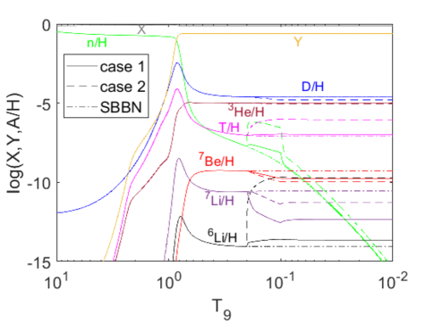
Figure 4: Nuclear abundances as a function of cosmic temperature $T_{9}=T/(10^{9}~{}\mathrm{K})$. Solid and dashed lines correspond to ($f_{\mathrm{dis}}$, $a_{\mathrm{dif}}$) = ($2\times 10^{-4}$, $0.1$) and ($2\times 10^{-4}$, $0.5$), respectively, in case B for magnetic field dissipation, while dash-dotted lines correspond to the standard model without a magnetic field. Cosmic ray generation at $T_{9}=0.2$–0.1 results in nonthermal nuclear reactions.

4 Conclusions

Nonthermal nuclear reactions induced by soft CRs originating from magnetic field dissipation in the early universe were investigated. We adopted two types of CR source spectra with reference to the observed spectra of solar energetic particles energized by solar magnetic fields. Our findings are as follows: The CR flux can be significantly high only after the completion of $e^{\pm}$ pair annihilation. Therefore, nonthermal nucleosynthesis affects primordial abundance after the annihilation epoch. The magnetic dissipation after the annihilation can explain the observations of the primordial Li and D abundances if the dissipated energy amounts to 0.01%–0.1% of the total cosmic energy. The CR source spectra should be very soft, so that D overdestruction is not triggered. When we assume that reconnection of large-scale magnetic fields with energy densities of 0.01%–0.1% of the total energy density generates jets of tightly coupled electron–nuclei plasma, the kinetic energies of the CR nuclei in the jets evolve and can temporarily match the order of 1 MeV/$A$ required to solve the Li problem.

Appendix A Momentum transfer rates and magnetic reconnection rate

We derive rough estimates of momentum transfer rates at $T_{9}=T/(10^{9}~{}{\rm K})=0.1$ with $T$ the temperature, after the electron annihilation in the Big Bang. The quantity $\sigma_{\mathrm{mt}}^{ab}$ defines the momentum transfer cross section (MTCS) of particle $a$ via the scattering off of particle $b$.

A.1 Electrons

The momentum exchange of electrons is dominated by Coulomb scatterings with $e^{-}$s in the early universe. The MTCS is then estimated considering scatterings off of target $e^{-}$ particles at rest in frame of the cosmic fluid under the nonrelativistic approximation. The maximum impact parameter $b_{\mathrm{max}}$ is set to the Debye length $\lambda_{\rm D}$ as

$$b_{\rm max} = \lambda_{\rm D}=4.58\times 10^{-3}~{}{\rm cm}~{}({\rm at}~{}T_{9}=0.1)$$ (A1)

$$\lambda_{\rm D} \approx \sqrt{\frac{T}{4\pi e^{2}\left(n_{e}+n_{\mathrm{b}}\right)}}~{}({\rm for}~{}T\lesssim m_{e}/26)$$ (A2)

$$= \sqrt{\frac{\pi}{8\zeta(3)\alpha\eta\left(2-Y_{\mathrm{p}}/2\right)T^{2}}},$$ (A3)

where $e$ and $m_{e}$ are the electronic charge and mass, respectively, $n_{e}$ and $n_{\mathrm{b}}$ are the electron and baryon number densities, respectively, $X_{\mathrm{p}}=0.75$ and $Y_{\mathrm{p}}=0.25$ are primordial mass fractions of ¹H and ⁴He, respectively, $n_{\gamma}=[2\zeta(3)/\pi^{2}]T^{3}$ is the photon number density with $\zeta(3)=1.2021$, $\eta=n_{\mathrm{b}}/n_{\gamma}=6\times 10^{-10}$ is the baryon-to-photon ratio, and $\alpha=e^{2}$ is the fine structure constant.

The scattering angle $\theta$ is related to the impact parameter $b$ by

$$b=\frac{q_{1}q_{2}e^{2}}{mv^{2}}\cot\left(\frac{\theta}{2}\right),$$ (A4)

where $q_{1}$ and $q_{2}$ are charge numbers of reacting particles 1 and 2, respectively, $m=m_{e}/2$ is the reduced mass, and $v$ is the $e^{-}$ velocity Then, the maximum of $\mu\equiv\cos{\theta}$ is given by

$$\mu_{\rm max} = \cos\theta_{\rm min}$$ (A5)

$$= \cos\left[2\cot^{-1}\left(b_{\rm max}\frac{m_{e}v^{2}}{2\alpha}\right)\right]$$ (A6)

$$\approx 1-3.04\times 10^{-20}v^{-4}~{}~{}(\mathrm{at}~{}T_{9}=0.1).$$ (A7)

With this maximum $\mu_{\rm max}$, the MTCS is given by

$$\sigma_{\rm mt}^{ee} \approx \int_{-1}^{\mu_{\rm max}}\frac{d\sigma}{d\mu}\frac{\Delta q_{e}}{q_{e}}d\mu$$ (A8)

$$\approx \frac{2^{1/2}\pi\alpha^{2}}{v^{2}q_{e}^{2}}\left[2(1-\mu_{\rm max})^{-1/2}\right]$$ (A9)

$$\approx 2.71\times 10^{6}/(vq_{e})^{2},$$ (A10)

where $q_{e}$ and $\Delta q_{e}=2q_{e}\sin(\theta/2)$ are the initial momentum and the momentum transfer of $e^{-}$, respectively, and the differential Mott cross section is given by

$$\frac{d\sigma}{d\mu}(v,\mu) = \frac{2\pi\alpha^{2}}{v^{2}{q_{e}}^{2}}\frac{1}{(1-\mu)^{2}}\left[1-\frac{v^{2}}{2}(1-\mu)\right].$$ (A11)

The momentum transfer rate of electrons via the Coulomb scattering is then given by

$$\Gamma_{\rm C}^{ee} \approx n_{e}\sigma_{\rm mt}^{ee}$$ (A12)

$$\sim \eta n_{\gamma}(1-Y_{\mathrm{p}}/2)\left[\frac{2.71\times 10^{6}}{(m_{e}v^{2})^{2}}\right]$$ (A13)

$$= 1.29\times 10^{9}~{}{\rm s}^{-1}v^{-4}~{}({\rm at}~{}T_{9}=0.1).~{}~{}~{}~{}~{}$$ (A14)

A.2 Nuclei

Scatterings are dominated by the Coulomb scattering with $e^{-}$. The maximum $\mu_{\mathrm{max}}$ is derived from Equation (A4) to be

$$\mu_{\rm max} = \cos\left[2\cot^{-1}\left(b_{\rm max}\frac{m_{e}v^{2}}{Z\alpha}\right)\right]$$ (A15)

$$\approx 1-7.61\times 10^{-21}Z^{2}v^{-4}~{}~{}(\mathrm{at}~{}T_{9}=0.1),$$ (A16)

where $Z$ is the atomic number of the nucleus. The MTCS of the nucleus is then given by

$$\sigma_{\rm mt}^{Ae} \approx \int_{-1}^{\mu_{\rm max}}\frac{d\sigma}{d\mu}\frac{\Delta q_{e}}{q_{e}}\frac{q_{e}}{q_{A}}d\mu$$ (A17)

$$\approx \frac{2^{3/2}\pi Z^{2}\alpha^{2}}{v^{2}q_{e}q_{A}}\left[2(1-\mu_{\rm max})^{-1/2}\right]$$ (A18)

$$\approx 1.08\times 10^{7}Z/(q_{e}q_{A}),$$ (A19)

where $q_{A}$ is the nuclear momentum. Accordingly, the momentum transfer rate is given by

$$\Gamma_{\rm C}^{Ae} \approx n_{e}\sigma_{\rm mt}^{Ae}$$ (A20)

$$\approx \eta n_{\gamma}(1-Y_{\mathrm{p}}/2)\left[\frac{1.08\times 10^{7}Z}{(m_{e}v)\sqrt{2m_{A}E_{A}}}\right]$$ (A21)

$$= \frac{1.69\times 10^{9}~{}{\rm s}^{-1}Z}{A^{1/2}v}\left(\frac{E_{A}}{3T/2}\right)^{-1/2}~{}({\rm at}~{}T_{9}=0.1),~{}~{}~{}~{}~{}$$ (A22)

where $A$ is the nuclear mass number, and $E_{A}$ is the nuclear kinetic energy.

The MTCS of electrons via scattering off of nuclei is, on the other hand, given by

$$\sigma_{\rm mt}^{eA} \approx \int_{-1}^{\mu_{\rm max}}\frac{d\sigma}{d\mu}\frac{\Delta q_{e}}{q_{e}}d\mu$$ (A23)

$$\approx \frac{2^{3/2}\pi Z^{2}\alpha^{2}}{v^{2}q_{e}^{2}}\left[2(1-\mu_{\rm max})^{-1/2}\right]$$ (A24)

$$\approx 1.08\times 10^{7}Z/q_{e}^{2}.$$ (A25)

Taking into account only the dominant contribution from proton scatterings, the momentum transfer rate of electrons via the proton scatterings is given by

$$\Gamma_{\rm C}^{ep} \approx n_{p}\sigma_{\rm mt}^{ep}$$ (A26)

$$\approx \eta n_{\gamma}(1-Y_{\mathrm{p}})\left[\frac{1.08\times 10^{7}}{(m_{e}v)^{2}}\right]$$ (A27)

$$= 4.42\times 10^{9}~{}{\rm s}^{-1}~{}v^{-2}~{}({\rm at}~{}T_{9}=0.1).$$ (A28)

A.3 Photons

When cosmic background radiation is exposed to a plasma composed of electrons and nuclei that has a bulk velocity $v_{\mathrm{out}}\ll 1$, the electrons lose momenta in the direction of the bulk velocity, identified as the $z$-direction, mainly via Compton scattering off the photons. The momentum transfer rate is given as follows. First, the rate of change in the average electron momentum in the $z$-direction, $p_{ez}$, is given by

$$\left|\frac{dp_{ez}}{dt}\right| \approx \frac{1}{n_{e}}\frac{2}{(2\pi)^{3}}\int d^{3}p_{e}f_{e}(\mbox{\boldmath$p$}_{e};T)\frac{2}{(2\pi)^{3}}\int d^{3}p_{\gamma}f(\mbox{\boldmath$p$}_{\gamma};T)$$ (A29)

$$\times\int_{-1}^{1}d\mu\frac{d\sigma_{\mathrm{Com}}}{d\mu}(\mu;\mbox{\boldmath$p$}_{e},\mbox{\boldmath$p$}_{\gamma})\frac{\int_{0}^{2\pi}d\phi\Delta p_{\gamma z}(\mu,\phi;\mbox{\boldmath$p$}_{e},\mbox{\boldmath$p$}_{\gamma})}{2\pi},$$

where $\mbox{\boldmath$p$}_{e}$ and $\mbox{\boldmath$p$}_{\gamma}$ are momenta of an electron and a photon, respectively, $f_{e}(\mbox{\boldmath$p$}_{e};T)$ and $f(\mbox{\boldmath$p$}_{\gamma};T)$ are the momentum distribution functions of electrons and photons, respectively, $d\sigma_{\mathrm{Com}}/d\mu$ is the differential cross section of the Compton scattering as a function of $\mu=\cos\theta$ for the scattering angle $\theta$, and $\Delta p_{\gamma z}$ is the increase of the $z$-component of the photon momentum $p_{\gamma z}$ that depends on the azimuthal angle $\phi$ at a scattering. The Pauli blocking of the electron and the induced emission of the photon have been neglected in this equation.

We assume an isotropic photon distribution in the cosmic rest frame and an isotropic electron distribution in the frame of the fluid moving in the rest frame. The electron distribution function in the cosmic rest frame is given (e.g. Kedia et al., 2021) by

$$f_{e}(\mbox{\boldmath$p$}_{e};T) = \frac{1}{\gamma_{V}}\left\{\exp\left[\frac{\gamma_{V}\left(E_{e}^{\mathrm{tot}}-Vp_{ez}\right)}{T}\right]+1\right\}^{-1},$$ (A30)

where $V$ is the bulk velocity of the fluid, $\gamma_{V}=(1-V^{2})^{-1/2}$, and $E^{\mathrm{tot}}_{e}$ is the total electron energy. When electrons are nonrelativistic and the second term in the exponent is much smaller than unity, this distribution is approximated by

$$f_{e}(p_{e},\mu_{e};T) \approx \frac{\exp(-\gamma_{V}E_{e}^{\mathrm{tot}}/T)}{\gamma_{V}}\left[1+\frac{\gamma_{V}Vp_{e}\mu_{e}}{T}\right],$$ (A31)

where $\mu_{e}=\cos\theta_{e}=p_{ez}/p_{e}$. Thus, a bulk velocity $V$ induces an excess in the distribution in the direction of $V$. For example, if $V\sim 0.05$ ($\gamma_{V}\sim 1$) and the electron kinetic energy $E_{e}=E^{\mathrm{tot}}_{e}-m_{e}\sim T$, the excess of $\mu_{e}=1$ at $T_{9}\sim 0.1$ is

$$\frac{\gamma_{V}Vp_{e}}{T} \sim V\sqrt{\frac{3m_{e}}{T}}\sim 0.6.$$ (A32)

Then, such jets include ${\mathcal{O}}(10)$% anisotropy in the distribution function of electrons.

For $T_{9}\lesssim 0.1$, background photon energies are much lower than the electron mass. By neglecting the photon energy shift at the Compton scattering as a perturbation of ${\mathcal{O}}(E_{\gamma}/m_{e})$, the differential cross section is reduced to that of the Thomson scattering, given by

$$\frac{d\sigma_{\mathrm{Com}}}{d\mu}(\mu) \approx \pi\left(\frac{e^{2}}{m_{e}}\right)^{2}\left(1+\mu^{2}\right).$$ (A33)

We define the $x$-axis so that the $zx$-plane includes $\mbox{\boldmath$p$}_{e}$ The change of $p_{\gamma z}$ is then given by

$$\Delta p_{\gamma z}(\mu,\phi;\mbox{\boldmath$p$}_{e},\mbox{\boldmath$p$}_{\gamma}) = E_{\gamma}^{\prime}\left[(\gamma\cos\theta_{e}\cos\psi-\sin\theta_{e}\cos\phi_{\gamma}\sin\psi)\cos\theta\right.$$ (A34)

$$-(\gamma\cos\theta_{e}\sin\psi+\sin\theta_{e}\cos\phi_{\gamma}\cos\psi)\sin\theta\cos\phi$$

$$\left.+\sin\theta_{e}\sin\phi_{\gamma}\sin\theta\sin\phi+\beta\gamma\cos\theta_{e}\right]-E_{\gamma}\gamma\cos\theta_{e}\cos\alpha_{\gamma},$$

where $E_{\gamma}$ and $E_{\gamma}^{\prime}$ are the energies of the photon in the cosmic rest frame before and after the scattering, respectively, $\beta$ is the electron velocity and $\gamma=(1-\beta^{2})^{-1/2}$, $\psi$ is the angle between $\mbox{\boldmath$p$}_{e}$ and $\mbox{\boldmath$p$}_{\gamma}^{(1)}$ that is the photon momentum in the rest frame of electron, $\phi_{\gamma}$ is the angle between the $x$-axis and the $\mbox{\boldmath$p$}_{\gamma}$ projected on the $xy$-plane, and $\alpha_{\gamma}$ is the angle between $\mbox{\boldmath$p$}_{e}$ and $\mbox{\boldmath$p$}_{\gamma}$. After the integration over $\phi$, terms proportional to $\sin\phi$ and $\cos\phi$ disappear. By neglecting terms of ${\mathcal{O}}(E_{\gamma}/m_{e})$ and ${\mathcal{O}}(\beta^{2})$, the remaining quantity becomes

$$\Delta p_{\gamma z}(\mu;\mbox{\boldmath$p$}_{e},\mbox{\boldmath$p$}_{\gamma}) \approx E_{\gamma}(1-\beta\cos\alpha_{\gamma})\left[(\cos\theta_{e}\cos\psi-\sin\theta_{e}\cos\phi_{\gamma}\sin\psi)\cos\theta+\beta\cos\theta_{e}\right]$$ (A35)

$$-E_{\gamma}\cos\theta_{e}\cos\alpha_{\gamma}.$$

The angle $\psi$ satisfies:

$$\cos\psi = \frac{\cos\alpha_{\gamma}-\beta}{v_{\mathrm{M}}}\approx\cos\alpha_{\gamma}-\beta\sin^{2}\alpha_{\gamma}$$ (A36)

$$\sin\psi \approx \sin\alpha_{\gamma}\left(1+\beta\cos\alpha_{\gamma}\right),$$ (A37)

where $v_{\mathrm{M}}=\sqrt{1-2\beta\cos\alpha_{\gamma}+\beta^{2}\cos^{2}\alpha_{\gamma}}$ is the Møller velocity. Then, after the integration over $\alpha_{\gamma}$, some terms including the last term in Equation (A35) disappear, and the remaining part is given by

$$\Delta p_{\gamma z}(\mu;p_{e},\cos\theta_{e},p_{\gamma}) \approx \beta E_{\gamma}\cos\theta_{e}\left(1-\mu\right).$$ (A38)

The term proportional to $\mu$ is significantly canceled when it is integrated over $\mu$. Then, the first term dominates, and the anisotropic electron distribution is reflected via this term to the momentum change rate.

The rate of change in the average value of $p_{ez}$ is then estimated as

$$\left|\frac{dp_{ez}}{dt}\right|\sim f_{\mathrm{exc}}n_{\gamma}(T)\sigma_{\mathrm{Th}}\left(v_{e,\mathrm{th}}E_{\gamma}\right),$$ (A39)

where $\sigma_{\mathrm{Th}}=(8\pi/3)(e^{2}/m_{e})^{2}=6.65\times 10^{-25}$ cm² is the Thomson scattering cross section, $v_{e,\mathrm{th}}=\sqrt{3T/m_{e}}$ is the thermal electron velocity, and $f_{\mathrm{exc}}$ is the excess fraction of electron flux moving downstream given by

$$f_{\mathrm{exc}} \sim \frac{\gamma_{v_{\mathrm{out}}}v_{\mathrm{out}}p_{e}}{T}$$ (A40)

$$\sim \mathcal{O}(0.1)\left(\frac{v_{\mathrm{out}}}{0.05}\right)\left(\frac{T_{9}}{0.1}\right)^{-1/2}.$$ (A41)

The momentum transfer rate of moving electrons via the scattering of background photons is derived with Equations (A39) and (A40) and $p_{e}\sim m_{e}v_{e,\mathrm{th}}$, as

$$\Gamma_{\mathrm{Th}}^{e\gamma} \sim \frac{|dp_{ez}/dt|}{m_{e}v_{\mathrm{out}}}$$ (A42)

$$\sim \frac{T}{m_{e}}n_{\gamma}(T)\sigma_{\mathrm{Th}}$$ (A43)

$$= 6.82\times 10^{9}~{}\mathrm{s}^{-1}\left(\frac{T_{9}}{0.1}\right)^{4}.$$ (A44)

The denominator on the right-hand side of Equation (A42) is the average electron momentum in a jet with a bulk velocity $v_{\mathrm{out}}$.

Then, energies generated at the magnetic reconnection are quickly shared among electrons and nuclei. For example, at $T_{9}=0.1$ and $v_{\mathrm{out}}\gtrsim 0.05$, the momentum transfer rates of electrons have the ordering of $\Gamma_{\mathrm{C}}^{ee}\gg\Gamma_{\mathrm{C}}^{ep}>\Gamma_{\mathrm{Th}}^{e\gamma}$. Therefore, after a large number of scatterings, bulk motions are expected to realize in jets composed of electrons and nuclei associated with a minor component of dragged photons.

A.4 dissipation scale

The dissipation of the primordial magnetic field over a length of $L$ dissipates on a time scale of $t=4\pi\sigma_{\mathrm{el}}L^{2}$, where $\sigma_{\mathrm{el}}$ is the electrical conductivity (Grasso & Rubinstein, 2001). Then, the magnetic fields over scales smaller than the maximum dissipation scale $L=\sqrt{t/(4\pi\sigma_{\mathrm{el}})}$ decay until a cosmic time $t$. The conductivity is given by

$$\sigma_{\mathrm{el}}=\frac{n_{e}e^{2}\tau_{\mathrm{mt}}^{ep}}{m_{e}},$$ (A45)

where $\tau_{\mathrm{mt}}^{ep}=(\Gamma_{\mathrm{C}}^{ep})^{-1}$ is the momentum transfer time scale of electrons. Using Equations (A24) and (A27), the maximum diffusion scale is transformed to

$$L = \left(\frac{m_{e}t\Gamma_{\mathrm{C}}^{ep}}{4\pi e^{2}n_{e}}\right)^{1/2}$$ (A46)

$$= \left(\left(\frac{m_{e}}{4\pi e^{2}}\right)\left\{\frac{2^{2}\pi\alpha^{2}}{v^{2}q_{e}^{2}}\left[1-\mu_{\rm max}(T)\right]^{-1/2}\right\}\left(\frac{3\sqrt{5}m_{\rm Pl}}{4\pi^{3/2}g_{\ast}^{1/2}T^{2}}\right)\right)^{1/2}$$ (A47)

$$\sim \left[\frac{\sqrt{10}}{8\pi^{3/2}}\frac{m_{e}m_{\rm Pl}\lambda_{\mathrm{D}}(T)}{g_{\ast}^{1/2}T^{3}}\right]^{1/2}$$ (A48)

$$= \left\{\frac{\sqrt{5}}{16\pi\left[\zeta(3)\alpha\right]^{1/2}}\frac{m_{e}m_{\rm Pl}}{g_{\ast}^{1/2}T^{4}\left[\eta\left(2-Y_{\mathrm{p}}/2\right)\right]^{1/2}}\right\}^{1/2},$$ (A49)

where $m_{\mathrm{Pl}}$ is the Planck mass, and $g_{\ast}=2+(21/4)(4/11)^{4/3}$ is the effective statistical degrees of freedom after the $e^{+}$–$e^{-}$ annihilation. The Debye length $\lambda_{\mathrm{D}}$ increases with decreasing $T$, and the maximum diffusion scale monotonically increases with decreasing $T$. At $T_{9}=0.1$, this scale corresponds to $L=18.4~{}\mathrm{km}~{}(T_{9}/0.1)^{-2}.$

A.5 Reconnection rate

The reconnection rate in the Sweet-Parker model (Sweet, 1958; Parker, 1957) is given by

$$\Gamma_{\mathrm{rec}} = \frac{v_{\mathrm{in}}}{L}=\frac{V_{\mathrm{A}}/L}{\sqrt{S}}=\left(\frac{V_{\mathrm{A}}\eta_{\mathrm{mag}}}{L^{3}}\right)^{1/2},$$ (A50)

where $v_{\mathrm{in}}$ is the inflow velocity of magnetic field lines into the reconnection region, $L$ is the size of the reconnection region, and $S$ is the Lundquist number defined as $S=V_{\mathrm{A}}L/\eta_{\mathrm{mag}}$, where $V_{\mathrm{A}}$ is the Alfvén velocity, and $\eta_{\mathrm{mag}}=1/(4\pi\sigma_{\mathrm{el}})$ is the magnetic diffusivity.

In the epoch after the $e^{+}e^{-}$ annihilation, electrons are dominantly scattered via Coulomb scattering by nuclei, except for self-scatterings. For example, at $T_{9}=0.1$, the thermal electron velocity is $v=\mathcal{O}(0.1)$, and the momentum transfer rate is $\Gamma_{\mathrm{C}}^{ep}\sim 10^{11}$ s^-1 (Equation (A28)). Under this condition, by using Equations (A25), (A26), and (A45), the reconnection rate is given by

$$\Gamma_{\mathrm{rec}} = \left(\frac{V_{\mathrm{A}}}{L^{3}}\frac{1}{4\pi}\frac{m_{e}\Gamma_{\mathrm{C}}^{ep}}{n_{e}e^{2}}\right)^{1/2}$$ (A51)

$$\sim \left(\frac{V_{\mathrm{A}}}{4\pi\alpha}\frac{m_{e}\sigma_{\mathrm{mt}}^{ep}}{L^{3}}\right)^{1/2}$$ (A52)

$$\sim \left(\frac{V_{\mathrm{A}}}{4\pi\alpha}\frac{1.08\times 10^{7}}{m_{e}v^{2}L^{3}}\right)^{1/2}.$$ (A53)

The Alfvén velocity for a relativistic plasma is given by

$$V_{\mathrm{A}} = \frac{B}{\sqrt{4\pi\left(\rho_{\mathrm{EM}}+P_{\mathrm{EM}}\right)}}$$ (A54)

$$\approx \sqrt{\frac{3f_{B}}{2f_{\mathrm{EM}}}},$$ (A55)

where $B$ is the magnetic field amplitude, $\rho_{\mathrm{EM}}$ and $P_{\mathrm{EM}}$ are the total energy density and pressure of electromagnetically coupled plasma in jets, respectively, $f_{B}=\rho_{B}/\rho_{\mathrm{rad}}$ is the ratio of the magnetic field energy density $\rho_{B}=B^{2}/(8\pi)$ to the total radiation energy density $\rho_{\mathrm{rad}}$, and $f_{\mathrm{EM}}=\rho_{\mathrm{EM}}/\rho_{\mathrm{rad}}$.

The dissipated energy is shared dominantly by electrons and nuclei. Then, the total energy in plasma jets is dominated by moving baryon energy. The energy density of the plasma is approximated by $\rho_{\mathrm{EM}}\simeq m_{\mathrm{b}}\gamma_{A}n_{\mathrm{b}}$, where $m_{\mathrm{b}}$ is the baryon mass, and $\gamma_{A}=(1-V_{A}^{2})^{-1/2}$. Then, it follows that

$$f_{\mathrm{EM}} = \frac{60\zeta(3)}{\pi^{4}g_{\ast}}\frac{m_{\mathrm{b}}}{T}\eta\gamma_{A}$$ (A56)

$$= 1.44\times 10^{-5}~{}\left(\frac{T_{9}}{0.1}\right)^{-1}\left(\frac{\eta}{6\times 10^{-10}}\right)\gamma_{A}.$$ (A57)

Therefore, if the field amplitude is as high as $f_{B}\sim 10^{-4}$–$10^{-3}$, the jets are highly relativistic with $V_{A}\sim 1$ and $\gamma_{A}\gg 1$.

Using Equation (A53) and $V_{A}\sim 1$, the reconnection rate is derived as

$$\Gamma_{\mathrm{rec}} = 2.03~{}{\rm s}^{-1}v^{-1}\left(\frac{L}{10~{}{\rm km}}\right)^{-3/2}.$$ (A58)

During the reconnection, jets involve surrounding background plasma, and bulk motions over large volumes would form. We roughly estimate a relation of the bulk velocity $v_{\mathrm{out}}$ and the reconnection region range $L$ as follows. By the reconnection, the magnetic field energy in the volume of $\sim L^{3}$ is converted to the energy of plasma jets ranging over a scale of $l_{\mathrm{jet}}\sim v_{\mathrm{out}}/\Gamma_{\mathrm{rec}}$. As a result, there is an energy conservation for nonrelativistic jets produced by the reconnection:

$$\rho_{B}L^{3}=\frac{\rho_{\mathrm{EM}}v_{\mathrm{out}}^{2}}{2}l_{\mathrm{jet}}^{3}=\frac{\rho_{\mathrm{EM}}v_{\mathrm{out}}^{5}}{2\Gamma_{\mathrm{rec}}^{3}}.$$ (A59)

Then, it follows with Equations (A57) and (A58) that

$$v_{\mathrm{out}} \sim \left[\frac{2\rho_{B}}{\rho_{\mathrm{EM}}}\left(\Gamma_{\mathrm{rec}}L\right)^{3}\right]^{1/5}$$ (A60)

$$= \left\{\frac{2f_{B}}{f_{\mathrm{EM}}}\left[20.3~{}\mathrm{km}~{}\mathrm{s}^{-1}v^{-1}\left(\frac{L}{10~{}{\rm km}}\right)^{-1/2}\right]^{3}\right\}^{1/5}$$ (A61)

$$\sim 8.45\times 10^{-3}\left(\frac{f_{B}}{10^{-3}}\right)^{1/5}\left(\frac{T_{9}}{0.1}\right)^{1/5}\left(\frac{\eta}{6\times 10^{-10}}\right)^{-1/5}\left(\frac{L}{10~{}{\rm km}}\right)^{-3/10}.$$ (A62)

Note that it is assumed that baryons in such extended jets are nonrelativistic. Thus, when the reconnection completes, the bulk velocity is small. During the reconnection, small and relativistic jets form first, and they gradually become large and slow. Nonthermal nucleosynthesis operates until the kinetic energies of nuclei in the jets become insufficient for inducing reactions.

A.6 Simple model

Figure 5 shows a schematic picture of the cosmic ray nucleosynthesis triggered by large-scale magnetic field reconnection, inferred from the estimates given above. Tightly coupled plasma of electrically-charged electrons and nuclei partially drags background photons at $T_{9}\sim 0.1$. Therefore, jets composed of electron-nuclei-photon fluid with a bulk velocity form. Depending on the magnetic field energy density, the kinetic energies of nuclei in the jets can be large enough that nonthermal nucleosynthesis effectively occurs when the jets collide with static background plasma.

Figure 5: Model of the cosmic ray nucleosynthesis triggered by the magnetic field reconnection. Magnetic reconnection converts the magnetic energy to the kinetic energy of charged particles. Because of the coupling of electrons, nuclei, and photons, plasma jets with bulk velocity $v_{\mathrm{out}}$ are formed. Nonthermal nucleosynthesis takes place where the jets are thermalized at their boundaries.

References

- Ade et al. (2017) Ade, P. A. R., et al. 2017, Phys. Rev. D, 96, 102003, doi: 10.1103/PhysRevD.96.102003
- Aghanim et al. (2020) Aghanim, N., et al. 2020, Astron. Astrophys., 641, A6, doi: 10.1051/0004-6361/201833910
- Aver et al. (2021) Aver, E., Berg, D. A., Olive, K. A., et al. 2021, Journal of Cosmology and Astroparticle Physics, 2021, 027, doi: 10.1088/1475-7516/2021/03/027
- Bania et al. (2002) Bania, T. M., Rood, R. T., & Balser, D. S. 2002, Nature, 415, 54, doi: 10.1038/415054a
- Coc et al. (2015) Coc, A., Petitjean, P., Uzan, J.-P., et al. 2015, Phys. Rev. D, 92, 123526, doi: 10.1103/PhysRevD.92.123526
- Cyburt et al. (2010) Cyburt, R. H., Amthor, A. M., Ferguson, R., et al. 2010, ApJS, 189, 240, doi: 10.1088/0067-0049/189/1/240
- Dimopoulos et al. (1988) Dimopoulos, S., Esmailzadeh, R., Hall, L. J., & Starkman, G. D. 1988, Astrophys. J., 330, 545, doi: 10.1086/166493
- Dolgov & Grasso (2002) Dolgov, A. D., & Grasso, D. 2002, Phys. Rev. Lett., 88, 011301, doi: 10.1103/PhysRevLett.88.011301
- Durrer & Neronov (2013) Durrer, R., & Neronov, A. 2013, Astron. Astrophys. Rev., 21, 62, doi: 10.1007/s00159-013-0062-7
- Fu et al. (2015) Fu, X., Bressan, A., Molaro, P., & Marigo, P. 2015, MNRAS, 452, 3256, doi: 10.1093/mnras/stv1384
- Fujiwara & Tang (1994) Fujiwara, Y., & Tang, Y. C. 1994, Few-Body Syst., 16, 91
- Gibbons & Macklin (1959) Gibbons, J. H., & Macklin, R. L. 1959, Phys. Rev., 114, 571, doi: 10.1103/PhysRev.114.571
- Grasso & Rubinstein (2001) Grasso, D., & Rubinstein, H. R. 2001, Phys. Rep., 348, 163, doi: 10.1016/S0370-1573(00)00110-1
- Greenstein (1969) Greenstein, G. 1969, Nature, 223, 938, doi: 10.1038/223938b0
- Hanayama et al. (2005) Hanayama, H., Takahashi, K., Kotake, K., et al. 2005, ApJ, 633, 941, doi: 10.1086/491575
- Hayakawa et al. (2021) Hayakawa, S., et al. 2021, Astrophys. J. Lett., 915, L13, doi: 10.3847/2041-8213/ac061f
- Ichiki et al. (2006) Ichiki, K., Takahashi, K., Ohno, H., Hanayama, H., & Sugiyama, N. 2006, Science, 311, 827, doi: 10.1126/science.1120690
- Jedamzik & Pogosian (2020) Jedamzik, K., & Pogosian, L. 2020, Phys. Rev. Lett., 125, 181302, doi: 10.1103/PhysRevLett.125.181302
- Kang et al. (2012) Kang, M.-m., Hu, Y., Hu, H.-b., & Zhu, S.-h. 2012, JCAP, 05, 011, doi: 10.1088/1475-7516/2012/05/011
- Kang et al. (2019) Kang, M.-M., Hu, Y., Hu, H.-B., & Zhu, S.-H. 2019, Astrophys. J., 873, 68, doi: 10.3847/1538-4357/ab0178
- Katz et al. (2021) Katz, H., et al. 2021. https://arxiv.org/abs/2101.11624
- Kawano (1992) Kawano, L. 1992
- Kawasaki et al. (2005) Kawasaki, M., Kohri, K., & Moroi, T. 2005, Phys. Rev. D, 71, 083502, doi: 10.1103/PhysRevD.71.083502
- Kawasaki & Kusakabe (2012) Kawasaki, M., & Kusakabe, M. 2012, Phys. Rev. D, 86, 063003, doi: 10.1103/PhysRevD.86.063003
- Kedia et al. (2021) Kedia, A., Sasankan, N., Mathews, G. J., & Kusakabe, M. 2021, Phys. Rev. E, 103, 032101, doi: 10.1103/PhysRevE.103.032101
- Kolb & Turner (1990) Kolb, E. W., & Turner, M. S. 1990, The Early Universe, Vol. 69
- Korn et al. (2006) Korn, A. J., Grundahl, F., Richard, O., et al. 2006, Nature, 442, 657, doi: 10.1038/nature05011
- Kusakabe et al. (2014) Kusakabe, M., Cheoun, M.-K., & Kim, K. S. 2014, Phys. Rev. D, 90, 045009, doi: 10.1103/PhysRevD.90.045009
- Kusakabe & Kawasaki (2013) Kusakabe, M., & Kawasaki, M. 2013, ApJ, 767, 5, doi: 10.1088/0004-637X/767/1/5
- Kusakabe & Kawasaki (2015) Kusakabe, M., & Kawasaki, M. 2015, Mon. Not. Roy. Astron. Soc., 446, 1597, doi: 10.1093/mnras/stu2115
- Lind et al. (2013) Lind, K., Melendez, J., Asplund, M., Collet, R., & Magic, Z. 2013, Astron. Astrophys., 554, A96, doi: 10.1051/0004-6361/201321406
- Luo et al. (2019) Luo, Y., Kajino, T., Kusakabe, M., & Mathews, G. J. 2019, Astrophys. J., 872, 172, doi: 10.3847/1538-4357/ab0088
- Minoda et al. (2019) Minoda, T., Tashiro, H., & Takahashi, T. 2019, Mon. Not. Roy. Astron. Soc., 488, 2001, doi: 10.1093/mnras/stz1860
- Nagai et al. (2006) Nagai, Y., Kobayashi, T., Shima, T., et al. 2006, Phys. Rev. C, 74, 025804, doi: 10.1103/PhysRevC.74.025804
- Parker (1957) Parker, E. N. 1957, J. Geophys. Res., 62, 509, doi: 10.1029/JZ062i004p00509
- Pitrou et al. (2018) Pitrou, C., Coc, A., Uzan, J.-P., & Vangioni, E. 2018, Phys. Rept., 754, 1, doi: 10.1016/j.physrep.2018.04.005
- Prantzos (2006) Prantzos, N. 2006, A&A, 448, 665, doi: 10.1051/0004-6361:20053897
- Ratra (1992) Ratra, B. 1992, ApJ, 391, L1, doi: 10.1086/186384
- Reames (2013) Reames, D. V. 2013, Space Sci. Rev, 175, 53, doi: 10.1007/s11214-013-9958-9
- Reno & Seckel (1988) Reno, M. H., & Seckel, D. 1988, Phys. Rev. D, 37, 3441, doi: 10.1103/PhysRevD.37.3441
- Sbordone et al. (2010) Sbordone, L., et al. 2010, Astron. Astrophys., 522, A26, doi: 10.1051/0004-6361/200913282
- Smith et al. (1993) Smith, M. S., Kawano, L. H., & Malaney, R. A. 1993, Astrophys. J. Suppl., 85, 219, doi: 10.1086/191763
- Spite & Spite (1982) Spite, F., & Spite, M. 1982, Astron. Astrophys., 115, 357
- Sweet (1958) Sweet, P. A. 1958, in Electromagnetic Phenomena in Cosmical Physics, ed. B. Lehnert, Vol. 6, 123
- Tilley et al. (2004) Tilley, D. R., Kelley, J. H., Godwin, J. L., et al. 2004, Nucl. Phys. A, 745, 155, doi: 10.1016/j.nuclphysa.2004.09.059
- Vachaspati (2021) Vachaspati, T. 2021, Rept. Prog. Phys., 84, 074901, doi: 10.1088/1361-6633/ac03a9
- Voronchev et al. (2012) Voronchev, V. T., Nakao, Y., Tsukida, K., & Nakamura, M. 2012, Phys. Rev. D, 85, 067301, doi: 10.1103/PhysRevD.85.067301
- Wang et al. (2021) Wang, M., Huang, W. J., Kondev, F. G., Audi, G., & Naimi, S. 2021, Chin. Phys. C, 45, 030003, doi: 10.1088/1674-1137/abddaf
- Yamada et al. (2010) Yamada, M., Kulsrud, R., & Ji, H. 2010, Reviews of Modern Physics, 82, 603, doi: 10.1103/RevModPhys.82.603
- Yamaguchi et al. (2013) Yamaguchi, H., et al. 2013, Phys. Rev. C, 87, 034303, doi: 10.1103/PhysRevC.87.034303
- Yamazaki (2018) Yamazaki, D. G. 2018, Phys. Rev. D, 97, 103525, doi: 10.1103/PhysRevD.97.103525
- Zavarygin et al. (2018) Zavarygin, E. O., Webb, J. K., Dumont, V., & Riemer-Sørensen, S. 2018, MNRAS, 477, 5536, doi: 10.1093/mnras/sty1003
- Zerkin & Pritychenko (2018) Zerkin, V. V., & Pritychenko, B. 2018, Nuclear Instruments and Methods in Physics Research A, 888, 31, doi: 10.1016/j.nima.2018.01.045
- Zyla et al. (2020) Zyla, P. A., et al. 2020, PTEP, 2020, 083C01, doi: 10.1093/ptep/ptaa104