Limits on sequential sharing of nonlocal advantage of quantum coherence

Abstract

Sequential sharing of nonlocal correlation is inherently related to its application. We address the question as to how many observers can share the nonlocal advantage of quantum coherence (NAQC) in a $(d\times d)$-dimensional state, where $d$ is a prime or a power of a prime. We first analyze the trade-off between disturbance and information gain of the general $d$-dimensional unsharp measurements. Then in a scenario where multiple Alices perform unsharp measurements on one party of the state sequentially and independently and a single Bob measures coherence of the conditional states on the other party, we show that at most one Alice can demonstrate NAQC with Bob. This limit holds even when considering the weak measurements with optimal pointer states. These results may shed light on the interplay between nonlocal correlations and quantum measurements on high-dimensional systems and the hierarchy of different quantum correlations.

I Introduction

The characteristics of a quantum state without any classical analog are fundamental and key issue of quantum physics Nielsen . Formally, one can introduce different forms of nonlocal correlations to characterize these intriguing characteristics, including Bell nonlocality confirming the nonexistence of the local hidden variable model Bell1 ; Bell2 , Einstein-Podolsky-Rosen (EPR) steering confirming the nonexistence of the local hidden state model steer1 ; steer2 , quantum entanglement originating from the superposition principle of states QE , and quantum discord which is rooted in the noncommutativity of operators QD . These nonlocal correlations are crucial physical resources for quantum communication and computation tasks which outperform their classical counterparts.

For a given quantum state, when one assumes no-signaling among its parties, the monogamy relation imposes constraints on the number of observers who can share the quantum correlations in this state monoe ; monon ; monos ; monoc ; monod . But if the no-signaling condition is partially relaxed, e.g., a single Bob holds half of an entangled pair, while multiple Alices (say, Alice₁, Alice₂, etc.) hold the other half of that pair and perform weak measurements sequentially and independently on their half, then the prior measurement of Alice₁ implicitly signals to Alice₂ by her choice of measurement setting, likewise, Alice₂ signals to Alice₃, and so on. Thereby the monogamy constraints might be relaxed to allow sequential sharing of quantum correlations. In this context, a double violation of the Clauser-Horne-Shimony-Holt (CHSH) inequality with equal sharpness of measurements has been theoretically predicted shareBT1 ; shareBT2 ; shareBT3 ; shareBT4 and experimentally verified shareBE1 ; shareBE2 ; shareBE3 . Further studies showed that an unbounded number of CHSH violations can be achieved using weak measurements with unequal sharpness shareBT6 ; shareBT7 ; shareBT8 . The weak measurement scenario has also been extended to investigate sequential sharing of tripartite Bell nonlocality shareBT9 , EPR steering shareST1 ; shareST2 ; shareST3 ; shareST4 , and bipartite entanglement shareET1 . Then an open question to ask is whether other forms of quantum correlations could be sequentially shared, especially for those beyond the two-qubit case or stronger than Bell nonlocality.

As a fundamental property in quantum theory, quantum coherence is not only an embodiment of the superposition principle of states, but is also intimately related to quantum correlations among the constituents of a system Ficek . In particular, following the resource theory of entanglement QE and quantum discord QD , Baumgratz et al. coher introduced a resource theoretic framework for quantifying coherence, within which the fascinating properties and potential applications of coherence have been investigated in a number of contexts Plenio ; Hu ; Wu ; ad1 ; ad2 ; ad3 . The resource theory of coherence can also be used to interpret those already known quantum correlations coen1 ; coen2 ; coen3 ; coqd1 ; coqd2 ; coqd3 ; coqd4 and introduce other quantifiers of correlations Hu , among which is the nonlocal advantage of quantum coherence (NAQC) naqc1 ; naqc2 . It is captured by violations of the coherence steering inequalities, which is similar to the Bell nonlocality captured by violation of the CHSH inequality CHSH . Specifically, for a $(d\times d)$-dimensional state $\rho_{AB}$ with $d$ being a power of a prime (hereafter, we call it the two-qudit state), when the steered coherence on $B$ after local measurements on $A$ exceeds a threshold, we say that there is NAQC in the sense that such a coherence is unattainable for any product state. As for its hierarchy with other quantum correlations, the set of states with NAQC forms a subset of entangled states naqc1 ; naqc2 and for the $d=2$ case, it is also a subset of Bell nonlocal states naqc3 .

In this work, we investigate how many Alices could sequentially demonstrate NAQC with a single Bob. We first analyze the information-disturbance trade-off of the $d$-dimensional unsharp measurements. Then in the context of unsharp measurements, we show that different from the sequential sharing of Bell nonlocality shareBT1 ; shareBT2 ; shareBT3 ; shareBT4 ; shareBE1 ; shareBE2 ; shareBE3 ; shareBT6 ; shareBT7 ; shareBT8 ; shareBT9 , EPR steering shareST1 ; shareST2 ; shareST3 ; shareST4 , and entanglement shareET1 , at most one Alice can demonstrate the NAQC with Bob. In particular, such a limit exists even when one considers the weak measurements with optimal pointer states. These results may enrich our comprehension on the interplay between NAQC and measurements on high-dimensional systems.

II Characterization of the NAQC

In 2014, Baumgratz et al. coher introduced a resource theoretic framework for quantifying coherence. Within this framework, the incoherent states are defined as those described by the diagonal density operators, and for a given state described by the density operator $\rho$, the amount of coherence could be quantified by its minimal distance to the set $\mathcal{I}$ of incoherent states in the same Hilbert space. By fixing the basis $\{|i\rangle\}$ which can be recognized as the normalized eigenbasis of a Hermitian operator $\mathcal{O}$, Baumgratz et al. coher further identified two coherence measures, that is, the $l_{1}$ norm and relative entropy of coherence, which are given by

$$C_{l_{1}}^{\mathcal{O}}(\rho)=\sum_{i\neq j}|\langle i|\rho|j\rangle|,~{}C_{re}^{\mathcal{O}}(\rho)=S(\rho_{\mathrm{diag}})-S(\rho),~{}$$ (1)

where the subscripts $l_{1}$ and $re$ indicate the metrics of the two coherence measures, while $S(\rho)$ and $S(\rho_{\mathrm{diag}})$ are the von Neumann entropies of $\rho$ and $\rho_{\mathrm{diag}}=\sum_{i}\langle i|\rho|i\rangle|i\rangle\langle i|$, respectively.

Starting from the above coherence measures, one can then introduce the NAQC which captures the nonlocal property of a bipartite state. Specifically, the NAQC characterizes the ability of one party to steer the coherence of the other one when they share a two-qudit state $\rho_{AB}$. To illustrate such a nonlocal characteristics, we suppose qudit $A$ ($B$) belongs to Alice (Bob) and denote by $\{A^{v}\}$ the set of $d+1$ mutually unbiased observables. Alice measures randomly one of the observables on qudit $A$ and informs Bob of her choice $A^{v}$ and outcome $a$. Then the conditional state of qudit $B$ will be given by

$$\rho_{B|\Pi^{v}_{a}}=\mathrm{Tr}_{A}[(\Pi^{v}_{a}\otimes\mathds{1})\rho_{AB}(\Pi^{v}_{a}\otimes\mathds{1})]/p_{\Pi^{v}_{a}},$$ (2)

where $\Pi^{v}=\{\Pi^{v}_{a}\}$ denotes the measurement operator of Alice, $\mathds{1}$ is the identity operator, and $p_{\Pi^{v}_{a}}=\mathrm{Tr}[(\Pi^{v}_{a}\otimes\mathds{1})\rho_{AB}]$ is the probability of Alice’s measurement outcome $a$.

After Alice’s local measurements, Bob can measure coherence of the conditional states on $B$ in different reference bases. In the first framework, Bob chooses with equal probability $1/d$ one of the eigenbasis of $\{A^{u}\}_{u\neq v}$, then one can obtain the average steered coherence (ASC) $N_{AB}^{\alpha}(\rho_{AB})$ ($\alpha=l_{1}$ or $re$) and the criterion for capturing NAQC in $\rho_{AB}$ is given by naqc1 ; naqc2

$$N_{AB}^{\alpha}(\rho_{AB})=\frac{1}{d}\sum_{u\neq v,a}p_{\Pi^{v}_{a}}C_{\alpha}^{A^{u}}(\rho_{B|\Pi^{v}_{a}})>N_{c}^{\alpha},$$ (3)

where the critical value $N_{c}^{\alpha}$ is obtained by first summing the single-qudit coherence over the $d+1$ mutually unbiased bases and then maximizing it over all the single-qudit states naqc2 . In the second framework, Bob chooses the eigenbasis of $A^{\beta_{v}}$ after Alice’s measurement $\Pi^{v}$, with $\beta=\{\beta_{v}\}_{v=0}^{d}$ being a permutation of the set $\{0,1,\ldots,d\}$ with elements $\beta_{v}$. Then the criterion for capturing NAQC in $\rho_{AB}$ becomes naqc2

$$\mathcal{N}_{AB}^{\alpha}(\rho_{AB})=\max_{\{\beta_{v}\}}\sum_{v,a}p_{\Pi^{v}_{a}}C_{\alpha}^{A^{\beta_{v}}}(\rho_{B|\Pi^{v}_{a}})>N_{c}^{\alpha},$$ (4)

where the maximum is taken over the $(d+1)!$ (the factorial of $d+1$) possible permutations of $\{0,1,\ldots,d\}$.

For the special $d=2$ case, the sharing of NAQC captured by the criterion of Eq. (3) has been studied sharenaqc ; sharenaqce . However, Eq. (3) is less efficient than Eq. (4) in capturing NAQC naqc2 , hence we will focus on the latter when discussing sharing of NAQC by sequential observers.

III Framework of unsharp measurements

In the framework of von Neumann-type measurement von , the measurement process on a $d$-dimensional state $\rho_{0}$ implies interaction of the system with the apparatus which induces the map: $\mathcal{E}(\rho_{0}\otimes|\phi\rangle\langle\phi|)=\sum_{ij}\Pi_{i}\rho_{0}\Pi_{j}\otimes|\phi_{i}\rangle\langle\phi_{j}|$, where $\{\Pi_{i}\}$ denotes the measurement operators, $|\phi\rangle$ is the initial pointer state of the apparatus, and $|\phi_{i}\rangle$ is the postmeasurement state of the pointer associated with the outcome $i$. By tracing out the pointer states one can obtain the nonselective postmeasurement state as $\rho=\sum_{ij}\Pi_{i}\rho_{0}\Pi_{j}\langle\phi_{i}|\phi_{j}\rangle$, where $\langle\phi_{i}|\phi_{j}\rangle$ may be different for different $i\neq j$. Without loss of generality, here we consider $\langle\phi_{i}|\phi_{j}\rangle\equiv F$ ($\forall i\neq j$) for simplicity, then $\rho$ can be reformulated as

$$\rho=F\rho_{0}+(1-F)\sum_{i}\Pi_{i}\rho_{0}\Pi_{i},$$ (5)

where $F\in[0,1]$ is the quality factor of the measurement, with $F=0$ corresponding to the usual projective (strong) measurement. $F$ measures the extent to which the system state remains undisturbed after the measurement and depends on the pointer of the apparatus by its definition shareBT1 .

One point to be stressed here is that the reduced disturbance of a weak measurement will induce reduced information gain. To quantify such a quantity (i.e., the information gain or precision of the measurements), one needs to choose a complete orthogonal set of states $\{|\varphi_{i}\rangle\}$ as reading states because the set $\{|\phi_{i}\rangle\}$ is non-orthogonal. As a result, the probability of getting the outcome $i$ and the associated (unnormalized) postmeasurement state $\rho_{i}=\langle\varphi_{i}|\mathcal{E}(\rho_{0}\otimes|\phi\rangle\langle\phi|)|\varphi_{i}\rangle$ are given by

$$p_{i}= \mathrm{Tr}(\Pi_{i}\rho_{0})|\langle\varphi_{i}|\phi_{i}\rangle|^{2}+\sum_{j\neq i}\mathrm{Tr}(\Pi_{j}\rho_{0})|\langle\varphi_{i}|\phi_{j}\rangle|^{2},$$ (6)

$$\rho_{i}= \Pi_{i}\rho_{0}\Pi_{i}|\langle\varphi_{i}|\phi_{i}\rangle|^{2}+\sum_{j\neq i}\Pi_{j}\rho_{0}\Pi_{j}|\langle\varphi_{i}|\phi_{j}\rangle|^{2}$$

$$+\sum_{m\neq n}\Pi_{m}\rho_{0}\Pi_{n}\langle\varphi_{i}|\phi_{m}\rangle\langle\phi_{n}|\varphi_{i}\rangle,$$

where $|\langle\varphi_{i}|\phi_{i}\rangle|^{2}$ ($|\langle\varphi_{i}|\phi_{j\neq i}\rangle|^{2}$) is the probability of obtaining the correct (wrong) outcome. When the measurement is unbiased, i.e., $|\langle\varphi_{i}|\phi_{i}\rangle|^{2}$ is independent of $i$ and $|\langle\varphi_{i}|\phi_{j\neq i}\rangle|^{2}$ is independent of $j\neq i$, Eq. (6) can be reformulated as

$$p_{i}= G\mathrm{Tr}(\Pi_{i}\rho_{0})+\frac{1-G}{d},$$ (7)

$$\rho_{i}= \frac{\mathcal{F}}{d}\rho_{0}+\frac{1+d_{1}G-\mathcal{F}}{d}\Pi_{i}\rho_{0}\Pi_{i}$$

$$+\frac{1-G-\mathcal{F}}{d}\left(\sum_{j\neq i}\Pi_{j}\rho_{0}\Pi_{j}+\sum_{m\neq n\atop m,n\neq i}\Pi_{m}\rho_{0}\Pi_{n}\right),$$

where $G=1-d|\langle\varphi_{i}|\phi_{j\neq i}\rangle|^{2}$ is the precision of the measurement which quantifies the information gain from the measured system and we have denoted by $\mathcal{F}=[(1+d_{1}G)(1-G)]^{1/2}$, where $d_{1}=d-1$. $G$ also depends on the pointer states of the measuring apparatus. Usually, one has the trade-off $F^{2}+G^{2}\leqslant 1$, and for $F^{2}+G^{2}=1$, the trade-off is said to be optimal in the sense that the measurement yields the highest precision for a given quality factor shareBT1 .

In this paper, we follow the framework of Refs. shareBT1 ; shareBT2 ; shareST2 and consider the $d$-dimensional unsharp measurements represented by the set of effect operators

$$E^{v}=\bigg{\{}E^{v}_{a}\mid E^{v}_{a}=\lambda\Pi^{v}_{a}+\frac{1-\lambda}{d}\mathds{1},a=0,1,\ldots,d-1\bigg{\}},$$ (8)

where $\{E^{v}_{a}\}$ represents the measurement settings with $d$ possible outcomes per setting, $0<\lambda\leqslant 1$ represents the sharpness parameter, and $\Pi^{v}_{a}=|\phi^{v}_{a}\rangle\langle\phi^{v}_{a}|$ is the projector. In the following, we restrict ourselves to $\Pi^{v}_{a}$ ($v=0,1,\ldots,d$) constructed by the $d+1$ mutually unbiased bases MUB1 ; MUB2 :

$$\left|\phi^{0}_{a}\right\rangle=\sum_{n=0}^{d-1}\delta_{an}|n\rangle,~{}\left|\phi^{d}_{a}\right\rangle=\frac{1}{\sqrt{d}}\sum_{n=0}^{d-1}e^{i\frac{2\pi}{d}an}|n\rangle,$$ (9)

$$\left|\phi^{r}_{a}\right\rangle=\frac{1}{\sqrt{d}}\sum_{n=0}^{d-1}e^{i\frac{2\pi}{d}r(a+n)^{2}}|n\rangle~{}(r=1,\ldots,d-1),$$

where $\delta_{an}$ is the Delta function and $i$ represents the imaginary unit. One can note that the unsharp measurement operator $E^{v}_{a}$ corresponds to a linear combination of the projector $\Pi^{v}_{a}$ with the white noise. It satisfies the relation $\sum_{a}E^{v}_{a}=\mathds{1}$ ($\forall v$) and belongs to the class of positive-operator-valued measurements. In contrast to the conventional strong measurement which enables an extraction of the maximum information and destroys completely the system to be measured, for the unsharp measurements the system is weakly coupled to the probe and thus provides less information about the system while producing less disturbance weak1 ; weak2 . Hence, the postmeasurement states retain some original properties of the measured system which might be observed by the subsequent observers. Moreover, $E^{v}_{a}$ reduces to the projective (strong) measurements when $\lambda=1$, and for such a special case, the basis comprising $\Pi^{v}_{a}$ is an essential ingredient for introducing the flag additivity condition which is equivalent to the strong monotonicity and convexity of a coherence measure new1 ; new2 .

Note that for $d=2$, the effect operators can also be written as $E_{\pm}=(\mathds{1}\pm\lambda\hat{n}\cdot\vec{\sigma})/2$, where $\hat{n}$ is a unit vector in $\mathbb{R}^{3}$ and $\vec{\sigma}$ is a vector composed of the three Pauli operators.

From Eq. (8) one can obtain that for any initial state $\rho_{0}$, the nonselective postmeasurement state is given by Luders

$$\rho=\sum_{a}\sqrt{E^{v}_{a}}\rho_{0}\sqrt{E^{v}_{a}}=\lambda_{0}\rho_{0}+(1-\lambda_{0})\sum_{a}\Pi^{v}_{a}\rho_{0}\Pi^{v}_{a},$$ (10)

and the probability of getting the outcome $a$ is given by

$$p_{E^{v}_{a}}=\mathrm{Tr}(E^{v}_{a}\rho_{0})=\lambda\mathrm{Tr}(\Pi^{v}_{a}\rho_{0})+\frac{1-\lambda}{d},$$ (11)

where

$$\lambda_{0}=\frac{1}{d}\left[(d-2)(1-\lambda)+2\sqrt{1+(d-2)\lambda-d_{1}\lambda^{2}}\right].$$ (12)

Then by comparing Eqs. (5) and (7) with Eqs. (10) and (11), one can see that the quality factor and precision of the unsharp measurements (8) are respectively given by

$$F=\lambda_{0},~{}G=\lambda.$$ (13)

Hence unsharpening the measurements with a parameter $\lambda$ enables the control of the trade-off between disturbance and information gain. For $d=2$, one always has the optimal trade-off $F^{2}+G^{2}=1$. But for the prime $d\geqslant 3$, $F^{2}+G^{2}\leqslant 1$, and the equality holds only for $\lambda=1$, which corresponds to $F=0$ and $G=1$, namely, the case of a projective (strong) measurement shareBT1 .

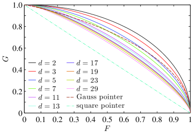
Figure 1: The trade-off between the quality factor $F$ and precision $G$ for the unsharp measurements (8). The solid lines from top to bottom correspond to the primes $d$ ranging from 2 to 29, where the topmost line for $d=2$ also corresponds to the optimal trade-off. For comparison, the trade-off for the Gauss pointer (dashed) and square pointer (dash-dotted) are also shown in this figure.

In Fig. 1 we give a plot of the trade-off between the quality factor $F$ and precision $G$ for the unsharp measurements of Eq. (8) with the first ten primes, and for comparison, we also show the trade-off for the Gauss pointer considered usually and the simple square pointer shareBT1 . For $d=2$, as mentioned before, it saturates the optimal trade-off constraint $F^{2}+G^{2}=1$, i.e., for any $F$, there exists optimal measurement pointer that achieves the maximum $G$ shareBT1 . For the prime $d\geqslant 3$, as shown in Fig. 1, although the corresponding trade-off is not optimal, it is still better than that given by the Gauss pointer for any $F$ (if $d=3$) or when $F$ is smaller than a threshold (if $d\geqslant 5$), and with an increase in $d$, it approaches gradually the trade-off $F+G=1$ given by the square pointer shareBT1 .

IV Sharing NAQC by sequential observers

To address the question for sequential sharing of the NAQC, we consider a scenario in which multiple Alices (say, Alice₁, Alice₂, etc.) have access to half of an entangled qudit pair and a spatially separated single Bob has access to the other half, and they agree on the measurement settings $\{E^{v}\}$ in prior shareBT1 . First, Alice₁ and Bob share the state $\rho_{A_{1}B}$ and Alice₁ proceeds by choosing randomly one of $\{E^{v}\}$ and performs the unsharp measurements on qudit $A_{1}$. She then passes the measured qudit (we rename it as qudit $A_{2}$) on to Alice₂ who measures again and passes it on to Alice₃, and so on until the last Alice. During the whole process, every Alice is assumed to be ignorant of the measurement settings chosen by the former Alices, that is, communications among them are forbidden and each Alice chooses independently and randomly one of the measurement setting. Our aim is to determine the maximum number of Alices whose statistics of measurements can demonstrate NAQC with a spatially separated single Bob.

IV.1 Sharing NAQC between Alice₁ and Bob

For the given $\rho_{A_{1}B}$, Alice₁ proceeds by choosing randomly the measurement setting $E^{v}$, performing the unsharp measurements (8) on $A_{1}$ and recording her outcomes. Then within the Lüders rule Luders , the selective postmeasurement states can be written as

$$\rho_{A_{1}B|E^{v}_{a}}=\left(\sqrt{E^{v}_{a}}\otimes\mathds{1}\right)\rho_{A_{1}B}\left(\sqrt{E^{v}_{a}}\otimes\mathds{1}\right)\big{/}p_{B|E^{v}_{a}},$$ (14)

where $p_{B|E^{v}_{a}}=\mathrm{Tr}[(E^{v}_{a}\otimes\mathds{1})\rho_{A_{1}B}]$ is the probability of the measurement outcome $a$, and the square roots of the unsharp measurements can be obtained as shareST2

$$\sqrt{E^{v}_{a}}=\left(\sqrt{\frac{1+d_{1}\lambda}{d}}-\sqrt{\frac{1-\lambda}{d}}\right)\Pi^{v}_{a}+\sqrt{\frac{1-\lambda}{d}}\mathds{1},$$ (15)

where as said before, we have defined $d_{1}=d-1$.

To proceed, we suppose that Alice₁ and Bob initially share the following maximally entangled two-qudit state

$$|\Psi\rangle_{A_{1}B}=\frac{1}{\sqrt{d}}\sum_{k=0}^{d-1}|kk\rangle,$$ (16)

then from Eq. (14) one can obtain the postmeasurement states $\rho_{A_{1}B|E^{v}_{a}}$ contingent upon Alice₁’s unsharp measurement $E^{v}$ on $A_{1}$ with outcome $a$. By further tracing over $A_{1}$ one can obtain the conditional states of qudit $B$ as

$$\rho_{B|E^{0}_{a}}=\frac{1-\lambda_{1}}{d}\mathds{1}+\lambda_{1}|a\rangle\langle a|,$$ (17)

$$\rho_{B|E^{d}_{a}}=\frac{1}{d}\mathds{1}+\frac{\lambda_{1}}{d}\sum_{n_{1,2}=0\atop n_{1}\neq n_{2}}^{d-1}e^{i\frac{2\pi}{d}a(n_{2}-n_{1})}|n_{1}\rangle\langle n_{2}|,$$

$$\rho_{B|E^{r}_{a}}=\frac{1}{d}\mathds{1}+\frac{\lambda_{1}}{d}\sum_{n_{1,2}=0\atop n_{1}\neq n_{2}}^{d-1}e^{i\frac{2\pi}{d}r\theta_{a,n_{1,2}}}|n_{1}\rangle\langle n_{2}|,$$

where $\lambda_{1}$ is the sharpness parameter of Alice₁, $r=1,\ldots,d-1$, and the probability of obtaining $\rho_{B|E^{v}_{a}}$ is given by $p_{B|E^{v}_{a}}=1/d$ ($\forall v,a$). Besides, we have defined $\theta_{a,n_{1,2}}=(a+n_{2})^{2}-(a+n_{1})^{2}$ for convenience of later presentation.

Table 1: Bob’s reference basis to measure the coherence of the collapsed states on qudit $B$, where $r=1,\ldots,d-1$.

  Bob’s collapsed state Bob’s reference basis $\rho_{B|E^{0}_{a}}$ $\{|\phi^{d}_{a}\rangle\}$ $\rho_{B|E^{d}_{a}}$ $\{|\phi^{0}_{a}\rangle\}$ $\rho_{B|E^{r}_{a}}$ $\{|\phi^{r}_{a}\rangle\}$  

The states $\rho_{B|E^{0}_{a}}$, $\rho_{B|E^{d}_{a}}$, and $\rho_{B|E^{r}_{a}}$ ($r=1,\ldots,d-1$) are diagonal in the bases $\{|\phi^{0}_{a}\rangle\}$, $\{|\phi^{d}_{a}\rangle\}$, and $\{|\phi^{d-r}_{a}\rangle\}$, respectively. For any $\rho_{B|E^{v}_{a}}$, its coherence in the basis $\{|\phi^{u}_{a}\rangle\}$ with $u\in\{0,1,\ldots,d\}$ are the same apart from the one mentioned above under which it is diagonal. So for convenience of later calculations, we assume that Bob chooses the bases $\{|\phi^{d}_{a}\rangle\}$, $\{|\phi^{0}_{a}\rangle\}$, and $\{|\phi^{r}_{a}\rangle\}$ to measure the coherences of $\rho_{B|E^{0}_{a}}$, $\rho_{B|E^{d}_{a}}$, and $\rho_{B|E^{r}_{a}}$, respectively (see Table 1). Then by transforming the collapsed states given in Eq. (17) to the bases shown in Table 1, one can obtain

$$\varrho_{B|E^{0}_{a}}=\frac{1}{d}\mathds{1}+\frac{\lambda_{1}}{d}\sum_{n_{1,2}=0\atop n_{1}\neq n_{2}}^{d-1}e^{i\frac{2\pi}{d}a(n_{2}-n_{1})}\left|\phi_{n_{1}}^{d}\right\rangle\left\langle\phi_{n_{2}}^{d}\right|,$$ (18)

$$\varrho_{B|E^{d}_{a}}=\frac{1}{d}\mathds{1}+\frac{\lambda_{1}}{d}\sum_{n_{1,2}=0\atop n_{1}\neq n_{2}}^{d-1}e^{i\frac{2\pi}{d}a(n_{2}-n_{1})}\left|\phi_{n_{1}}^{0}\right\rangle\left\langle\phi_{n_{2}}^{0}\right|,$$

$$\varrho_{B|E^{r}_{a}}=\frac{1}{d}\mathds{1}+\frac{\lambda_{1}}{d^{2}}\sum_{n_{1,2}=0\atop n_{1}\neq n_{2}}^{d-1}\sum_{k_{1,2}=0}^{d-1}e^{i\frac{2\pi}{d}r\varphi_{a,k_{1,2},n_{1,2}}}\left|\phi_{n_{1}}^{r}\right\rangle\left\langle\phi_{n_{2}}^{r}\right|,$$

where $\varphi_{a,k_{1,2},n_{1,2}}=\theta_{a,k_{1,2}}+(k_{2}+n_{2})^{2}-(k_{1}+n_{1})^{2}$.

The eigenvalues of $\rho_{B|E^{v}_{a}}$ ($\forall v,a$) are $\epsilon_{0}=(1+d_{1}\lambda_{1})/d$ with degeneracy $1$ and $\epsilon_{1}=(1-\lambda_{1})/d$ with degeneracy $d_{1}$. Then in the scenario where Alice₁ chooses $E^{v}$ with probability $p_{A|E^{v}}=1/(d+1)$ ($\forall v$), the two forms of ASC attainable by Bob could be obtained as

$$\mathcal{N}^{l_{1}}_{A_{1}B}= (d^{2}-1)\lambda_{1},$$ (19)

$$\mathcal{N}^{re}_{A_{1}B}= \frac{d+1}{d}\big{[}(1+d_{1}\lambda_{1})\log_{2}(1+d_{1}\lambda_{1})$$

$$+d_{1}(1-\lambda_{1})\log_{2}(1-\lambda_{1})\big{]}.$$

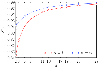
Figure 2: The critical sharpness parameter $\lambda_{1,c}^{\alpha}$ ($\alpha=l_{1}$ or $re$) stronger than which Alice₁ can demonstrate NAQC with Bob versus the prime $d$.

From Eq. (19) one can obtain the critical sharpness parameter $\lambda_{1,c}^{l_{1}}=\sqrt{d/(d+1)}$ stronger than which Alice₁ can demonstrate the $l_{1}$ norm of NAQC with Bob. Similarly, one can obtain numerically the critical $\lambda_{1,c}^{re}$ stronger than which Alice₁ can demonstrate the relative entropy of NAQC with Bob. In Fig. 2, we give a plot of the critical $\lambda_{1,c}^{\alpha}$ versus the prime $d$. It is clear that it always increases with an increase in $d$. Besides, it follows from Eqs. (13) and (19) that for any fixed prime $d$, $\mathcal{N}^{\alpha}_{A_{1}B}$ ($\alpha=l_{1}$ or $re$) is solely determined by the precision of the unsharp measurements of Alice₁.

IV.2 Sharing NAQC between Alice₂ and Bob

To proceed, we see whether the measurement statistics of two Alices can demonstrate NAQC with Bob. As we consider a sequential steering scenario, after finishing the unsharp measurement $E^{v}$, Alice₁ passes the measured qudit $A_{1}$ on to Alice₂ who is independent of her, namely, the classical information regarding the measurement setting and the outcome of Alice₁ is not conveyed. Then according to the Lüders transformation rule Luders , the state she shared with Bob can be written as

$$\rho_{A_{2}B|E^{v}}=\sum_{a=0}^{d-1}\left(\sqrt{E^{v}_{a}}\otimes\mathds{1}\right)\rho_{A_{1}B}\left(\sqrt{E^{v}_{a}}\otimes\mathds{1}\right),$$ (20)

where we have denoted by $\rho_{A_{2}B|E^{v}}$ the output state of Alice₁’s unsharp measurements $E^{v}=\{E^{v}_{a}\}$. Then for $\rho_{A_{1}B}$ of Eq. (16), one can obtain

$$\rho_{A_{2}B|E^{0}}=\lambda_{0}\rho_{A_{1}B}+\frac{1-\lambda_{0}}{d}\sum_{n=0}^{d-1}|nn\rangle\langle nn|,$$ (21)

$$\rho_{A_{2}B|E^{d}}=\lambda_{0}\rho_{A_{1}B}+\frac{1-\lambda_{0}}{d^{3}}\sum_{n,n_{1,2},\atop k_{1,2}=0}^{d-1}e^{i\frac{2\pi}{d}\xi_{n,n_{1,2},k_{1,2}}}|n_{1}n_{2}\rangle\langle k_{1}k_{2}|,$$

$$\rho_{A_{2}B|E^{r}}=\lambda_{0}\rho_{A_{1}B}+\frac{1-\lambda_{0}}{d^{3}}\sum_{n,n_{1,2},\atop k_{1,2}=0}^{d-1}e^{i\frac{2\pi}{d}r\zeta_{n,n_{1,2},k_{1,2}}}|n_{1}n_{2}\rangle\langle k_{1}k_{2}|,$$

where $\lambda_{0}$ can be obtained directly by substituting $\lambda$ in Eq. (12) with $\lambda_{1}$ and we have defined

$$\xi_{n,n_{1,2},k_{1,2}}=n(n_{1}-n_{2}-k_{1}+k_{2}),$$ (22)

$$\zeta_{n,n_{1,2},k_{1,2}}=\theta_{n,n_{1,2}}-\theta_{n,k_{1,2}}.$$

After receiving the qudit from Alice₁, Alice₂ performs the measurements $\{E^{v}_{a}\}$ on it (we rename it as qudit $A_{2}$) with the sharpness parameter $\lambda_{2}$. As Alice₂ is assumed to be ignorant of the measurement setting chosen by Alice₁ when measuring the qudit which is now in her possession, she has to consider the average effect of all possible measurement settings of Alice₁, that is, the NAQC Alice₂ shared with Bob has to be averaged over the $d+1$ possible outputs of Alice₁ given in Eq. (21).

First, for $\rho_{A_{2}B|E^{0}}$, one can obtain the selective postmeasurement states $\rho_{B|E^{0}E^{v}_{a}}$ ($v=0,1,\ldots,d$) of Bob after Alice₂’s unsharp measurement $\{E^{v}_{a}\}$ on qudit $A_{2}$, whose forms are similar to $\rho_{B|E^{v}_{a}}$ in Eq. (17). To be explicit, one could obtain $\rho_{B|E^{0}E^{0}_{a}}$ ($\rho_{B|E^{0}E^{d}_{a}}$ and $\rho_{B|E^{0}E^{r}_{a}}$) by substituting the parameter $\lambda_{1}$ in $\rho_{B|E^{0}_{a}}$ ($\rho_{B|E^{d}_{a}}$ and $\rho_{B|E^{r}_{a}}$) with $\lambda_{2}$ ($\lambda_{0}\lambda_{2}$). Thereby, the $l_{1}$ norm of coherence for $\rho_{B|E^{0}E^{0}_{a}}$ is $d_{1}\lambda_{2}$ and that for both $\rho_{B|E^{0}E^{d}_{a}}$ and $\rho_{B|E^{0}E^{r}_{a}}$ is $d_{1}\lambda_{0}\lambda_{2}$. Thus the $l_{1}$ norm of ASC attainable from $\rho_{A_{2}B|E^{0}}$ can be obtained as

$$\mathcal{N}^{l_{1}}_{A_{2}B|E^{0}}(\rho_{A_{2}B|E^{0}})=d_{1}(1+d\lambda_{0})\lambda_{2}.$$ (23)

Moreover, the eigenvalues of $\rho_{B|E^{0}E^{0}_{a}}$ can be obtained as $\varepsilon_{0}=(1+d_{1}\lambda_{2})/d$ with degeneracy $1$ and $\varepsilon_{1}=(1-\lambda_{2})/d$ with degeneracy $d_{1}$, while those for $\rho_{B|E^{0}E^{d}_{a}}$ and $\rho_{B|E^{0}E^{r}_{a}}$ can be obtained directly by substituting $\lambda_{2}$ in $\varepsilon_{0,1}$ with $\lambda_{0}\lambda_{2}$, hence the relative entropy of ASC for $\rho_{A_{2}B|E^{0}}$ can be obtained as

$$\mathcal{N}^{re}_{A_{2}B|E^{0}}(\rho_{A_{2}B|E^{0}})= (1+d)\log_{2}d-H_{2}\left(\frac{1+d_{1}\lambda_{2}}{d}\right)$$ (24)

$$-d_{1}\left(1-\lambda_{0}\lambda_{2}+\frac{1-\lambda_{2}}{d}\right)\log_{2}d_{1}$$

$$-dH_{2}\left(\frac{1+d_{1}\lambda_{0}\lambda_{2}}{d}\right),$$

where $H_{2}(\cdot)$ is the binary Shannon entropy function.

Next, for $\rho_{A_{2}B|E^{d}}$ of Eq. (21), the selective postmeasurement state $\rho_{B|E^{d}E^{d}_{a}}$ of qudit $B$ after Alice₂’s measurement $\{E^{d}_{a}\}$ is similar to $\rho_{B|E^{d}_{a}}$ in Eq. (17), with however the parameter $\lambda_{1}$ being replaced by $\lambda_{2}$, while the postmeasurement state $\rho_{B|E^{d}E^{0}_{a}}$ ($\rho_{B|E^{d}E^{r}_{a}}$) of Bob after Alice₂’s measurement $\{E^{0}_{a}\}$ ($\{E^{r}_{a}\}$) is similar to $\rho_{B|E^{0}_{a}}$ ($\rho_{B|E^{r}_{a}}$) of Eq. (17), with however the parameter $\lambda_{1}$ being replaced by $\lambda_{0}\lambda_{2}$. As a result, the $l_{1}$ norm and relative entropy of ASCs attainable from $\rho_{A_{2}B|E^{d}}$ have the same form as that given in Eqs. (23) and (24), respectively.

Finally, for $\rho_{A_{2}B|E^{r}}$ with $r=1,\ldots,d-1$, the selective postmeasurement state $\rho_{B|E^{r}E^{0}_{a}}$ ($\rho_{B|E^{r}E^{d}_{a}}$) of qudit $B$ after Alice₂’s measurement $\{E^{0}_{a}\}$ ($\{E^{d}_{a}\}$) on qudit $A_{2}$ is similar to $\rho_{B|E^{0}_{a}}$ ($\rho_{B|E^{d}_{a}}$) in Eq. (17), with however the parameter $\lambda_{1}$ being replaced by $\lambda_{0}\lambda_{2}$. In addition, the selective postmeasurement state $\rho_{B|E^{r}E^{s}_{a}}$ ($s=1,\ldots,d-1$) of qudit $B$ after Alice₂’s measurement $\{E^{s}_{a}\}$ on qudit $A_{2}$ can be obtained as

$$\rho_{B|E^{r}E^{s}_{a}}= \frac{1}{d}\mathds{1}+\frac{\lambda_{2}}{d}\sum_{n_{1,2}=0\atop n_{1}\neq n_{2}}^{d-1}\Bigg{[}\lambda_{0}e^{i\frac{2\pi}{d}s\theta_{a,n_{1},n_{2}}}$$ (25)

$$+\frac{1-\lambda_{0}}{d^{2}}\sum_{n,k_{1,2}=0}^{d-1}e^{i\frac{2\pi}{d}\varsigma_{a,n,k_{1,2},n_{1,2}}}\Bigg{]}|n_{1}\rangle\langle n_{2}|,$$

then by transforming it to the reference basis $\{|\phi^{s}_{a}\rangle\}$ (see Table 1), one has

$$\varrho_{B|E^{r}E^{s}_{a}}= \frac{1}{d}\mathds{1}+\frac{\lambda_{2}}{d^{2}}\sum_{n_{1,2}=0\atop n_{1}\neq n_{2}}^{d-1}\Bigg{[}\lambda_{0}\sum_{k_{1,2}=0}^{d-1}e^{i\frac{2\pi}{d}s\varphi_{a,k_{1,2},n_{1,2}}}$$ (26)

$$+\frac{1-\lambda_{0}}{d^{2}}\sum_{n,j_{1,2}\atop k_{1,2}=0}^{d-1}e^{i\frac{2\pi}{d}\chi_{a,n,j_{1,2},k_{1,2},n_{1,2}}}\Bigg{]}\left|\phi_{n_{1}}^{s}\right\rangle\left\langle\phi_{n_{2}}^{s}\right|,$$

where we have defined

$$\varsigma_{a,n,k_{1,2},n_{1,2}}= s\theta_{a,k_{1,2}}-r(\theta_{n,k_{1,2}}+\theta_{n,n_{1,2}}),$$ (27)

$$\chi_{a,n,j_{1,2},k_{1,2},n_{1,2}}= r(\theta_{n,k_{1,2}}-\theta_{n,j_{1,2}})+s[(a+k_{2})^{2}$$

$$-(a+j_{2})^{2}+(n_{2}+k_{1})^{2}-(n_{1}+j_{1})^{2}].$$

For $\varrho_{B|E^{r}E^{s}_{a}}$ of Eq. (26), the $l_{1}$ norm of coherence is given by $d_{1}\lambda_{2}$ for $s=r$ and $d_{1}\lambda_{0}\lambda_{2}$ for $s\neq r$. Similarly, the eigenvalues of $\varrho_{B|E^{r}E^{s}_{a}}$ for $s=r$ are $\varepsilon_{0}=(1+d_{1}\lambda_{2})/d$ with degeneracy $1$ and $\varepsilon_{1}=(1-\lambda_{2})/d$ with degeneracy $d-1$, while the eigenvalues of $\varrho_{B|E^{r}E^{s}_{a}}$ for $s\neq r$ could be obtained directly by substituting $\lambda_{2}$ in $\varepsilon_{0,1}$ with $\lambda_{0}\lambda_{2}$. Then after some algebra, one can obtain that the $l_{1}$ norm and relative entropy of ASCs attainable from $\rho_{A_{2}B|E^{r}}$ also have the same form as that given in Eqs. (23) and (24), respectively.

Since we are concerned with an unbiased input scenario, all the possible measurement settings of Alice₁ are equiprobable, i.e., her probability of choosing the measurement setting $E^{v}$ is $p_{A|E^{v}}=1/(d+1)$ ($\forall v$), thus the steerable coherence for Alice₂ and Bob can be obtained as

$$\mathcal{N}^{\alpha}_{A_{2}B}=\sum_{v}p_{A|E^{v}}\mathcal{N}^{\alpha}_{A_{2}B|E^{v}}(\rho_{A_{2}B|E^{v}}),$$ (28)

where $\alpha=l_{1}$ or $re$. By substituting $p_{A|E^{v}}=1/(d+1)$ and the associated ASC for $\rho_{A_{2}B|E^{0}}$, $\rho_{A_{2}B|E^{d}}$, and $\rho_{A_{2}B|E^{r}}$ ($r=1,\ldots,d-1$) into Eq. (28), one can obtain

$$\mathcal{N}^{l_{1}}_{A_{2}B}= d_{1}(1+d\lambda_{0})\lambda_{2},$$ (29)

$$\mathcal{N}^{re}_{A_{2}B}= (1+d)\log_{2}d-d_{1}\left(1-\lambda_{0}\lambda_{2}+\frac{1-\lambda_{2}}{d}\right)\log_{2}d_{1}$$

$$-H_{2}\left(\frac{1+d_{1}\lambda_{2}}{d}\right)-dH_{2}\left(\frac{1+d_{1}\lambda_{0}\lambda_{2}}{d}\right).$$

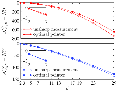
Figure 3: $\mathcal{N}^{\alpha}_{A_{2}B}-N^{\alpha}_{c}$ ($\alpha=l_{1}$ or $re$) versus the prime $d$ with $\lambda_{1}=\lambda_{1,c}^{\alpha}$ and $\lambda_{2}=1$. Their dependence on small $d$ are also shown in the insets to better visual the behavior.

As mentioned before, $\lambda_{0}$ depends on $\lambda_{1}$, so $\mathcal{N}^{\alpha}_{A_{2}B}$ ($\alpha=l_{1}$ or $re$) for Alice₂ and Bob is determined by both the quality factor of Alice₁’s measurements and the precision of Alice₂’s measurements. Eq. (29) also reveals that $\mathcal{N}^{\alpha}_{A_{2}B}$ decreases with the increasing disturbance (i.e., increasing precision) of Alice₁’s measurements and for any fixed disturbance of Alice₁, Alice₂ can enhance $\mathcal{N}^{\alpha}_{A_{2}B}$ by improving the precision of her measurements. Under the condition of guaranteeing the observation of NAQC for Alice₁ and Bob, $\mathcal{N}^{\alpha}_{A_{2}B}$ takes its maximum when the measurement of Alice₂ is sharp (i.e., $\lambda_{2}=1$) and the sharpness parameter $\lambda_{1}$ of Alice₁ is a slightly stronger than $\lambda_{1,c}^{\alpha}$. In Fig. 3 we show the $d$ dependence of $\mathcal{N}^{\alpha}_{A_{2}B}-N^{\alpha}_{c}$ with $\lambda_{1}=\lambda_{1,c}^{\alpha}$ and $\lambda_{2}=1$ (the hollow circles). It can be seen that it decreases with the increase of the prime $d$ and is always smaller than 0. This indicates that when Alice₁ steers successfully the NAQC on Bob’s side, Alice₂ will cannot steer it again.

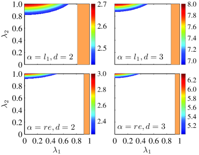
Figure 4: Plot of $\mathcal{N}^{\alpha}_{A_{2}B}$ ($\alpha=l_{1}$ or $re$) in the parameter region $(\lambda_{1},\lambda_{2})$ in which Alice₂ can steer the NAQC on Bob for $d=2$ and 3, and in the orange shaded regions, Alice₁ can steer the NAQC on Bob (note that Alice₁’s ability to steer the NAQC is independent of $\lambda_{2}$).

Having clarified the fact that Alice₂ cannot steer the NAQC on qudit $B$ when Alice₁ steers it successfully, it is definite that the subsequent Alices (i.e., Alice_n with $n\geqslant 3$) also can never steer the NAQC. Now, the issue that remains is whether Alice₂ can steer the NAQC after Alice₁’s unsharp measurements with $0<\lambda_{1}\leqslant\lambda_{1,c}^{\alpha}$, namely, Alice₁’s measurements are unable to extract enough information to observe the NAQC. To address this precisely, we further display in Fig. 4 dependence of $\mathcal{N}^{\alpha}_{A_{2}B}$ ($\alpha=l_{1}$ or $re$) on $\lambda_{1}$ and $\lambda_{2}$ for two primes $d=2$ and 3, and in the same figure we also show the regions of $\lambda_{1}$ in which Alice₁ can steer the NAQC on qudit $B$. Looking at this figure, one can see that there exists parameter region $(\lambda_{1},\lambda_{2})$ in which Alice₂ can steer the NAQC, and to ensure Alice₂’s steerability of the NAQC, the sharpness parameter $\lambda_{1}$ of Alice₁’s measurements should be weaker than a threshold $\lambda_{1,t}^{\alpha}$. From Fig. 4 one can also note that such a parameter region shrinks with an increase in the prime $d$. In particular, in the region of $\lambda_{1}\in[\lambda_{1,t}^{\alpha},\lambda_{1,c}^{\alpha}]$, both Alice₁ and Alice₂ cannot steer the NAQC, that is, Alice₁ should tune the sharpness of her measurement, as an unappropriate strength of measurement will prevent both of them from demonstrating the NAQC. All these show evidently that no matter how the sharpness parameters $\lambda_{1}$ and $\lambda_{2}$ are chosen, at most one Alice (i.e., Alice₁ or Alice₂) can demonstrate NAQC with a spatially separated Bob.

By comparing Eqs. (19) and (29) one can further note that $\mathcal{N}^{\alpha}_{A_{1}B}$ and $\mathcal{N}^{\alpha}_{A_{2}B}$ show an opposite dependence on $\lambda_{1}$. That is to say, the enhancement of Alice₁’s steerable coherence implies the degradation of Alice₂’s, and vice versa. In some sense, one may recognize this as a kind of sequentially monogamous characteristics of NAQC, as it sets limit on the possibility for Alice₁ and Alice₂ to steer the NAQC with Bob simultaneously, even if the resource state is maximally entangled.

Note that for the $d=2$ case, our results also apply to NAQC captured by the criterion of Eq. (3), the sequential sharing of which has been discussed in Ref. sharenaqc ; sharenaqce . But there are minor errors in sharenaqce related to the relative entropy of NAQC.

As we showed above, for the unbiased inputs of Alice₂ (i.e., equiprobable measurement settings for Alice₁), it is impossible for the NAQC of an entangled pair of qudits be distributed between two Alices who act sequentially and independently of each other. Then another interesting question to ask is whether Alice₂ could demonstrate NAQC when the inputs to her are biased. This question is important by itself as Alice₂ is ignorant of Alice₁’s measurement setting, thereby her premeasurement state is a mixture of the collapsed states of Alice₁’s possible measurements weighted by their probabilities. To answer this question, we resort again to the amounts of steered coherence discussed above for $\rho_{A_{2}B|E^{v}}$ ($v=0,1,\ldots,d$) of Eq. (21). As mentioned before, the different $\rho_{A_{2}B|E^{v}}$ yields the same steerable coherence, thus even there is input bias for Alice₂, it does not change the limit that it is impossible for more than one Alice to demonstrate NAQC with Bob.

It is also relevant to ask whether the above conclusion also holds in a scenario where Alice₁ measures the qudit $A_{1}$ with unequal sharpness, e.g., Alice₁ performs the measurement $E^{v}$ with sharpness parameter $\lambda_{1,v}$. In this case, following the similar derivations as in the previous sections, one can show that Alice₂ still cannot demonstrate NAQC with Bob if Alice₁ can do so. For example, when $d=2$ and Alice₂’s measurement is sharp, one has

$$\mathcal{N}_{A_{1}B}^{l_{1}}=\sum_{v}\lambda_{1,v},~{}\mathcal{N}_{A_{2}B}^{l_{1}}=1+\frac{2}{3}\sum_{v}\sqrt{1-\lambda_{1,v}^{2}},$$ (30)

then one can show that the maximal NAQC for Alice₂ and Bob corresponds to $\lambda_{1,v}=\lambda_{1}$ ($\forall v$). Thus she still cannot demonstrate NAQC with Bob.

One may also be concerned with the issue that whether the number of Alices sequentially sharing the NAQC could be enhanced when we consider the weak measurement with optimal pointer shareBT1 . For $d=2$, as said, it is already optimal. For the general prime $d$, by using Eq. (7) and after some algebra similar to those for the unsharp measurements, it can be found that although $\mathcal{N}^{\alpha}_{A_{2}B}$ can be enhanced to some extent (see the solid circles in Fig. 3), it still cannot exceed $N^{\alpha}_{c}$ under the condition of $\mathcal{N}^{\alpha}_{A_{1}B}>N_{c}^{\alpha}$. This confirms again that at most one Alice can demonstrate NAQC with Bob. But it should be note that although there is no NAQC in the postmeasurement states of Eq. (21), there are still other forms of residual quantum correlations. For example, for the $d=2$ case, when $\mathcal{N}_{A_{1}B}^{l_{1}}=2.50$, one can get a $14.26\%$ violation of the CHSH inequality for all the postmeasurement states of Alice₁ CHSH .

Lastly, when $d$ is a power of a prime, a complete set of $d+1$ mutually unbiased bases also exists MUB2 , and one can show in a similar way that all the above results also apply to this case. But as the NAQC were defined only for $d$ being a prime or a prime power naqc2 , the formulation of NAQC and its sequential sharing for a general $d$ are still open questions.

V Conclusion

In conclusion, we have investigated sequential sharing of NAQC in the $(d\times d)$-dimensional (i.e., two-qudit) state, with $d$ being a power of a prime. We consider these high-dimensional states, as compared with the two-dimensional ones, not only enrich our comprehension of the nonlocal characteristics in quantum theory but also show many advantages in quantum communication tasks such as the high channel capacity and security adv1 ; adv2 ; adv3 ; adv4 ; adv5 . By considering a scenario in which multiple Alices perform their unsharp measurements sequentially and independently of each other on the same half of an entangled qudit pair and a single Bob measures coherence of the collapsed states on the other half, we showed that for both the metrics (i.e., the $l_{1}$ norm and relative entropy) used for quantifying coherence and for both the unbiased and biased input scenarios, at most one Alice can demonstrate NAQC with Bob. Moreover, we showed that the conclusion also holds even when one considers the weak measurements with the optimal pointer, even when Alice₁’s measurement settings are biased, or when she measures the qudit with unequal sharpness associated with different measurement settings.

The results presented above indicate that there exists a strict limit on the number of Alices whose statistics of measurements can demonstrate NAQC with a spatially separated Bob. This provides an alternative dimension in the context of sequential sharing of quantum correlations and might shed light on the interplay between quantum measurement and quantum correlations for high-dimensional states. Furthermore, in the sense that the maximum number of observers being able to sequentially sharing quantum correlations is inherently related to the hierarchy of the strengths of quantum correlations, for example, Bell-CHSH nonlocality could be shared by not more than two unbiased observers shareBT1 ; shareBT2 ; shareBT3 and EPR steering could be shared by at most $n$ observers when the steering inequality based on $n$ measurement settings is used shareST1 ; shareST2 , it is intuitive to conjecture that the observation that the NAQC can be shared by at most one observer might indicate that it characterizes a kind of quantum correlation which is stronger than Bell nonlocality for the general two-qudit states, just as that for the two-qubit states naqc3 . Of course, further study is still needed to provide a rigorous proof of this conjecture. As there are other coherence measures Plenio ; Hu , deriving the associated criteria for capturing NAQC and exploring whether they could provide an advantage over those considered in this work in the context of NAQC sharing is another direction for future studies. Moreover, how such a strong quantum correlation can be used in practical communication and computation tasks would also be worth pursuing in the future.

References

- (1) M. A. Nielsen, and I. L. Chuang, Quantum Computation and Quantum Information (Cambridge University Press, Cambridge, UK, 2010).
- (2) Genovese M, Phys. Rep. 413, 319 (2005).
- (3) N. Brunner, D. Cavalcanti, S. Pironio, V. Scarani, and S. Wehner, Rev. Mod. Phys. 86, 419 (2014).
- (4) D. Cavalcanti, and P. Skrzypczyk, Rep. Prog. Phys. 80, 024001 (2017).
- (5) R. Uola, A. C. S. Costa, H. C. Nguyen, and O. Gühne, Rev. Mod. Phys. 92, 015001 (2020).
- (6) R. Horodecki, P. Horodecki, M. Horodecki, and K. Horodecki, Rev. Mod. Phys. 81, 865 (2009).
- (7) K. Modi, A. Brodutch, H. Cable, Z. Paterek, and V. Vedral, Rev. Mod. Phys. 84, 1655 (2012).
- (8) V. Coffman, J. Kundu, and W. K. Wootters, Phys. Rev. A 61, 052306 (2000).
- (9) B. Toner, Proc. R. Soc. London A 465, 59 (2009).
- (10) M. D. Reid, Phys. Rev. A 88, 062108 (2013).
- (11) L. Lami, C. Hirche, G. Adesso, and A. Winter, Phys. Rev. Lett. 117, 220502 (2016).
- (12) A. Streltsov, G. Adesso, M. Piani, and D. Bruß, Phys. Rev. Lett. 109, 050503 (2012).
- (13) R. Silva, N. Gisin, Y. Guryanova, and S. Popescu, Phys. Rev. Lett. 114, 250401 (2015).
- (14) S. Mal, A. S. Majumdar, and D. Home, Mathematics 4, 48 (2016).
- (15) C. Ren, T. Feng, D. Yao, H. Shi, J. Chen, and X. Zhou, Phys. Rev. A 100, 052121 (2019).
- (16) D. Das, A. Ghosal, S. Sasmal, S. Mal, and A. S. Majumdar, Phys. Rev. A 99, 022305 (2019).
- (17) M. J. Hu, Z. Y. Zhou, X. M. Hu, C. F. Li, G. C. Guo, and Y. S. Zhang, npj Quantum Inf. 4, 63 (2018).
- (18) M. Schiavon, L. Calderaro, M. Pittaluga, G. Vallone, and P. Villoresi, Quantum Sci. Technol. 2, 015010 (2017).
- (19) T. Feng, C. Ren, Y. Tian, M. Luo, H. Shi, J. Chen, and X. Zhou, Phys. Rev. A 102, 032220 (2020).
- (20) P. J. Brown, and R. Colbeck, Phys. Rev. Lett. 125, 090401 (2020).
- (21) T. Zhang, and S. M. Fei, Phys. Rev. A 103, 032216 (2021).
- (22) S. Cheng, L. Liu, T. J. Baker, and M. J. W. Hall, Phys. Rev. A 104, L060201 (2021).
- (23) S. Saha, D. Das, S. Sasmal, D. Sarkar, K. Mukherjee, A. Roy, and S. S. Bhattacharya, Quantum Inf. Process. 18, 42 (2019).
- (24) S. Sasmal, D. Das, S. Mal, and A. S. Majumdar, Phys. Rev. A 98, 012305 (2018).
- (25) A. Shenoy H., S. Designolle, F. Hirsch, R. Silva, N. Gisin, and N. Brunner, Phys. Rev. A 99, 022317 (2019).
- (26) D. Yao, and C. Ren, Phys. Rev. A 103, 052207 (2021).
- (27) X. H. Han, Y. Xiao, H. C. Qu, R. H. He, X. Fan, T. Qian, and Y. J. Gu, Quantum Inf. Process. 20, 278 (2021).
- (28) A. Bera, S. Mal, A. Sen(De), and U. Sen, Phys. Rev. A 98, 062304 (2018).
- (29) Z. Ficek, and S. Swain, Quantum Interference and Coherence: Theory and Experiments (Springer Series in Optical Sciences, Springer, Berlin, 2005).
- (30) T. Baumgratz, M. Cramer, and M. B. Plenio, Phys. Rev. Lett. 113, 140401 (2014).
- (31) A. Streltsov, G. Adesso, and M. B. Plenio, Rev. Mod. Phys. 89, 041003 (2017).
- (32) M. L. Hu, X. Hu, J. C. Wang, Y. Peng, Y. R. Zhang, and H. Fan, Phys. Rep. 762–764, 1 (2018).
- (33) K. D. Wu, A. Streltsov, B. Regula, G. Y. Xiang, C. F. Li, and G. C. Guo, Adv. Quantum Technol. 4, 2100040 (2021).
- (34) M. L. Hu, and H. Fan, Sci. China-Phys. Mech. Astron. 63, 230322 (2020).
- (35) L. M. Zhang, T. Gao, and F. L. Yan, Sci. China-Phys. Mech. Astron. 64, 260312 (2021).
- (36) Z. X. Jin, L. M. Yang, S. M. Fei, X. Li-Jost, Z. X. Wang, G. L. Long, and C. F. Qiao, Sci. China-Phys. Mech. Astron. 64, 280311 (2021).
- (37) A. Streltsov, U. Singh, H. S. Dhar, M. N. Bera, and G. Adesso, Phys. Rev. Lett. 115, 020403 (2015).
- (38) X. Qi, T. Gao, and F. Yan, J. Phys. A 50, 285301 (2017).
- (39) K. C. Tan, H. Kwon, C. Y. Park, and H. Jeong, Phys. Rev. A 94, 022329 (2016).
- (40) Y. Yao, X. Xiao, L. Ge, and C. P. Sun, Phys. Rev. A 92, 022112 (2015).
- (41) M. L. Hu, and H. Fan, Phys. Rev. A 95, 052106 (2017).
- (42) X. Hu, and H. Fan, Sci. Rep. 6, 34380 (2016).
- (43) X. Hu, A. Milne, B. Zhang, and H. Fan, Sci. Rep. 6, 19365 (2015).
- (44) D. Mondal, T. Pramanik, and A. K. Pati, Phys. Rev. A 95, 010301 (2017).
- (45) M. L. Hu, and H. Fan, Phys. Rev. A 98, 022312 (2018).
- (46) J. F. Clauser, M. A. Horne, A. Shimony, and R. A. Holt, Phys. Rev. Lett. 23, 880 (1969).
- (47) M. L. Hu, X. M. Wang, and H. Fan, Phys. Rev. A 98, 032317 (2018).
- (48) S. Datta, and A. S. Majumdar, Phys. Rev. A 98, 042311 (2018).
- (49) S. Datta, and A. S. Majumdar, Phys. Rev. A 99, 019902 (2019).
- (50) J. von Neumann, Mathematical Foundations of Quantum Mechanics (Princeton University Press, Princeton, 2018).
- (51) W. K. Wooters, Found. Phys. 16, 391 (1986).
- (52) W. K. Wooters, and B. D. Fields, Ann. Phys. 191, 363 (1989).
- (53) Y. Aharonov, D. Z. Albert, and L. Vaidman, Phys. Rev. Lett. 60, 1351 (1988).
- (54) I. M. Duck, P. M. Stevenson, and E. C. G. Sudarshan, Phys. Rev. D 40, 2112 (1989).
- (55) X. D. Yu, D. J. Zhang, G. F. Xu, and D. M. Tong, Phys. Rev. A 94, 060302 (2016).
- (56) C. L. Liu, X. D. Yu, and D. M. Tong, Phys. Rev. A 99, 042322 (2019).
- (57) P. Busch, Phys. Rev. D 33, 2253 (1986).
- (58) X. M. Hu, J. S. Chen, B. H. Liu, Y. Guo, Y. F. Huang, Z. Q. Zhou, Y. J. Han, C. F. Li, and G. C. Guo, Phys. Rev. Lett. 117, 170403 (2016).
- (59) X. M. Hu, Y. Guo, B. H. Liu, Y. F. Huang, C. F. Li, and G. C. Guo, Sci. Adv. 4, eaat9304 (2018).
- (60) X. M. Hu, W. B. Xing, B. H. Liu, Y. F. Huang, C. F. Li, G. C. Guo, P. Erker, and M. Huber, Phys. Rev. Lett. 125, 090503 (2020).
- (61) X. M. Hu, C. Zhang, B. H. Liu, Y. Cai, X. J. Ye, Y. Guo, W. B. Xing, C. X. Huang, Y. F. Huang, C. F. Li, and G. C. Guo, Phys. Rev. Lett. 125, 230501 (2020).
- (62) X. M. Hu, W. B. Xing, B. H. Liu, D. Y. He, H. Cao, Y. Guo, C. Zhang, H. Zhang, Y. F. Huang, C. F. Li, and G. C. Guo, Optica 7, 738 (2020).