Topology-Preserving Dimensionality Reduction via Interleaving Optimization

Abstract

Dimensionality reduction techniques are powerful tools for data preprocessing and visualization which typically come with few guarantees concerning the topological correctness of an embedding. The interleaving distance between the persistent homology of Vietoris-Rips filtrations can be used to identify a scale at which topological features such as clusters or holes in an embedding and original data set are in correspondence. We show how optimization seeking to minimize the interleaving distance can be incorporated into dimensionality reduction algorithms, and explicitly demonstrate its use in finding an optimal linear projection. We demonstrate the utility of this framework to data visualization.

Keywords Dimensionality Reduction  $\cdot$ Interleaving Distance  $\cdot$ Persistent Homology

1 Introduction

Dimension reduction is an important component of many data analysis tasks, but can be potentially problematic as it may “reveal” structure in data which is not truly present. In inference this can be addressed by principled use of a withheld test set or an analysis which addresses model selection more directly. However, in exploratory data analysis it can be difficult to address selection problems incurred by exploration of different dimension reduction techniques, such as whether visualized structures are really present or an artifact of the chosen embedding. In this paper, we develop the use of the interleaving distance for the purpose of quantifying the extent to which topological features of an embedding relate to features in the original data set. Explicitly, we can compute a threshold after which features of a certain size in the persistent homology of the Vietoris-Rips filtration are in one-to-one correspondence between the data set before and after dimension reduction. Furthermore, we show how to find local minima of this threshold through optimization and demonstrate this on the task of finding optimal projections of a data set.

1.1 Related Work

Optimization of persistent homology-based objective functions has attracted much recent attention [29, 17, 19, 22, 6, 5, 26] with a particular focus on applications in computational geometry and deep learning. Of particular relevance is the work of [27] which uses a persistence-based objective to preserve critical edges in the persistent homology of the Vietoris-Rips filtration in a learned latent space of an autoencoder.

The idea of using persistent homology to compare different dimension reduction schemes was initiated by Rieck and Leitte [30, 31], which uses the $2$-Wasserstein distance to compare the persistence diagrams of a data set before and after dimension reduction. Several non-differentiable methods incorporating persistent homology have been developed [12, 36, 13]. With the development of optimization techniques for persistent homology, several differentiable methods have been proposed based on optimization of the $2$-Wasserstein metric on persistence diagrams [20, 34] and an approach based on simulated annealing [37]. While not employed on Vietoris-Rips filtrations, the work of [29] uses the bottleneck distance for optimization of functional maps on shapes.

The interleaving/bottleneck distance has long been a key tool developed for the study of persistent homology under perturbation of the input [9]. The interleaving distance was first introduced by [7], and applied to the study of Vietoris-Rips filtrations in [8] to bound the distance of persistent homology by the Gromov-Hausdorff distance between the input point clouds. The idea of developing confidence regions for persistence pairs was developed by [15] in the context of sampling.

1.2 Contributions

This work presents a novel approach to dimension reduction using optimization of the interleaving/bottleneck distance between the persistent homology of Vietoris-Rips Filtrations of an original data set $X$ and the data set $Y$ after dimensionality reduction.

1. We show how the interleaving distance can be used to quantify a scale at which topological features in $X$ and features in $Y$ are in correspondence, and be used to select homological features of $Y$ in correspondence with features in $X$.

2. We show how to incorporate the interleaving distance explicitly into the optimization of the embedding $Y$ and prove the existence of descent directions under mild conditions.

3. We demonstrate this technique in finding optimal linear projections of the data set $X$ to preserve the bottleneck distance on several examples with interesting topology.

2 Background

2.1 Persistent Homology of Vietoris-Rips Filtrations

We are interested in discovering and preserving topological features of a point cloud $X$ together with a notion of dissimilarity $d$, and refer to the combination of these two data as a dissimilarity space $(X,d)$. A dissimilarity is a function $d:X\times X\to\mathbb{R}_{\geq 0}$, with $d(x,x)=0$ for any $x\in X$. We will typically consider dissimilarities that are metrics (in particular which satisfy triangle inequality), but many of the bounds here hold more generality. Examples of topological features of the space $(X,d)$ include clusters formed through single-linkage clustering or “holes” forming loops in the $r$-nearest neighbors graph of $X$.

Vietoris-Rips filtrations are commonly used in conjunction with persistent homology to create features for finite dimensional metric spaces (point clouds) [2]. Given a dissimilarity space $(X,d)$, a Vietoris-Rips complex consists of simplices with a maximum pairwise dissimilarity between vertices is less than some threshold $r$ :

$$X_{r}=\left\{\left(x_{0},\ldots,x_{k}\right)\mid x_{i}\in X,d\left(x_{i},x_{j}\right)\leq r\right\}$$

A Vietoris-Rips filtration is a nested sequence of Vietoris-Rips complexes $X_{r}\subseteq X_{s}$ if $r\leq s$.

Homology is a functor from the category of topological spaces and continuous maps to the category of vector spaces and linear maps (for a general introduction see [18]). The dimension of the $k$-dimensional homology vector space $H_{k}(X)$ of a topological space $X$ counts $k$-dimensional topological features of $X$: $\dim H_{0}(X)$ is the number of connected components, $\dim H_{1}(X)$ counts loops, and $\dim H_{k}$ generally counts $k$-dimensional voids. A continuous map $f:X\to Y$ has an induced map $H_{k}(f):H_{k}(X)\to H_{k}(Y)$ which maps vectors associated with topological features in $X$ to vectors associated with topological features in $Y$. The computation of $H_{k}(X)$ begins with the construction of a chain complex $C_{\ast}(X)=\{C_{k}(X),\partial_{k}:C_{k}(X)\to C_{k-1}(X)\}_{k\geq 0}$ where $C_{k}(X)$ is a vector space with a basis element for each $k$-simplex in $X$, and the boundary map $\partial_{k}$ sends each basis element to a linear combination of basis elements of faces in the boundary of the associated simplex. The boundary maps satisfy $\partial_{k}\circ\partial_{k+1}=0$, and $H_{k}(X)$ is the quotient vector space $\ker\partial_{k}/\operatorname{img}\partial_{k+1}$.

Persistent homology [14, 38] is an algebraic invariant of filtrations which captures how the topology of a filtration changes using homology. The output of persistent homology is a persistence vector space $V_{\ast}$, consisting of vector spaces $\{V_{r}=H_{k}(X_{r})\}_{r\in\mathbb{R}}$ and linear maps induced by inclusion $\{\iota^{V}_{r,s}:V_{r}\to V_{s}\}_{r\leq s\in\mathbb{R}}$ which satisfy a consistency condition $\iota^{V}_{r,t}=\iota^{V}_{r,s}\iota^{V}_{s,t}$ for all $r\leq s\leq t$.

Persistence vector spaces are classified up to isomorphism by birth-death pairs $\{(b_{i},d_{i})\}_{i\in I}$, or equivalently their persistence barcode [38] or interval indecomposables [3]. Each pair $(b,d)$ is associated to the appearance of a new homology vector at filtration parameter $b$ (meaning it is not in the image of an induced map), which maps through the persistence vector space until it enters the kernel of an induced map at filtration parameter $d$. The length of the pair $(b,d)$ is the difference $|d-b|$.

Every birth and death in persistent homology is associated with the addition of a particular simplex in the filtration. This follows from the definition of homology of the quotient vector space $H_{k}(X)=\ker\partial_{k}/\operatorname{img}\partial_{k+1}$. The addition of a new $k$-simplex increases the dimension of $C_{k}(X)$ by one, and either increases the dimension of $\ker\partial_{k}$ by one, causing a birth in $H_{k}(X)$, or increases the dimension of $\operatorname{img}\partial_{k}$ by one, causing a death in $H_{k-1}(X)$. Because the Vietoris-Rips filtration is determined by its edges, the filtration value of every simplex can be mapped to the largest pairwise distance. This provides a way to map the gradient of a function with respect to births and deaths to a gradient with respect to each pairwise distance – see [17] for additional details.

2.2 The Interleaving and Bottleneck Distances

Interleavings allow for the comparison of two persistence vector spaces [7], as well as other objects filtered by some partially ordered set [1]. Let $V_{\ast}$ and $W_{\ast}$ be 1-parameter persistence vector spaces. An $\epsilon$-shift map $f_{\ast}:V_{\ast}\to W_{\ast}$ is a collection of maps $f_{r}:V_{r}\to W_{r+\epsilon}$ so that the following diagram commutes for all parameters $r$

(1)

An $\epsilon$-interleaving between $V_{\ast}$ and $W_{\ast}$ is a pair of $\epsilon$-shift maps $f_{\ast}:V_{\ast}\to W_{\ast}$ and $g_{\ast}:W_{\ast}\to V_{\ast}$ so that $g_{r+\epsilon}f_{r}=\iota^{V}_{r,r+2\epsilon}$ and $f_{r+\epsilon}g_{r}=\iota^{W}_{r,r+2\epsilon}$ for all parameters $r$.

The interleaving distance [7] on persistence modules $V_{\ast}$ and $W_{\ast}$ is

$$d_{\mathrm{I}}(V_{\ast},W_{\ast})=\inf\{\epsilon\geq 0\mid\text{$V_{\ast}$ and $W_{\ast}$ are $\epsilon$-interleaved}\}$$ (2)

This notion of distance satisfies triangle inequality through the composition of interleavings. Note that the addition or removal an arbitrary number of zero-length pairs to a persistence vector space $V_{\ast}$ to obtain $V^{\prime}_{\ast}$ results in $d_{I}(V_{\ast},V^{\prime}_{\ast})=0$.

The construction of general interleavings, let alone those that would realize the interleaving distance, can be a daunting task. Fortunately, for 1-parameter persistent homology the interleaving distance $d_{I}$ is equivalent to the geometric (and easily computable) bottleneck distance $d_{B}$ on persistence diagrams [25].

The bottleneck distance considers the birth-death pairs $\{(b_{i},d_{i})\}_{i\in I}$ as points in the 2-dimensional plane. The persistence diagram $\operatorname{dgm}(V_{\ast})$ is the union of this discrete multi-set of the points $\{(b_{i},d_{i})\}$ with the diagonal $\Delta=\{(x,x)\mid x\in\mathbb{R}\}$ where points in $\Delta$ are counted with infinite multiplicity.

Definition 2.1.

A matching between two persistence diagrams $\operatorname{dgm}_{1}$ and $\operatorname{dgm}_{2}$ is a subset $\Omega\subseteq\operatorname{dgm}_{1}\times\operatorname{dgm}_{2}$ such that every points in $\operatorname{dgm}_{1}\setminus\Delta$ and $\operatorname{dgm}_{2}\setminus\Delta$ appears exactly once in $m$.

Definition 2.2.

The Bottleneck distance between $\operatorname{dgm}_{1}$ and $\operatorname{dgm}_{2}$ is then defined by

$$\mathrm{d}_{\mathrm{B}}\left(\operatorname{dgm}_{1},\operatorname{dgm}_{2}\right)=\inf_{\text{matching }}\max_{(p,q)\in\Omega}\|p-q\|_{\infty}$$ (3)

The bottleneck distance on persistence diagrams is isometric to the interleaving distance on persistence vector spaces, which is a result known as the isometry theorem:

Theorem 2.3.

[25] Let $\operatorname{dgm}(V_{\ast})$ and $\operatorname{dgm}(W_{\ast})$ be the persistent diagrams of $V_{\ast}$ and $W_{\ast}$ respectively. Then

$$d_{\mathrm{I}}(V_{\ast},W_{\ast})=d_{\mathrm{B}}(\operatorname{dgm}(V_{\ast}),\operatorname{dgm}(W_{\ast}))$$

The matching in the bottleneck distance actually gives an interleaving which maps a vector associated to a persistence pair in $\operatorname{dgm}(V_{\ast})$ to the vector associated with the matched pair in $\operatorname{dgm}(W_{\ast})$ which realizes the interleaving distance.

2.3 Bounds on the Interleaving Distance

In practice, persistent homology of the Vietoris-Rips filtration can be quickly approximated using sub-sampling. Bounds on this approximation come from the Hausdorff or Gromov-Hausdorff distance on between point clouds [8].

Definition 2.4.

The Hausdorff distance between two subsets $X$ and $Y$ within the same metric space is

$$d_{H}(X,Y)=\max\left\{\sup_{x}\inf_{y}\|x-y\|_{\infty},\sup_{y}\inf_{x}\|y-x\|_{\infty}\right\}$$

Definition 2.5.

A correspondence between two sets $X$ and $Y$ is a subset $C\subset X\times Y$ such that: $\forall x\in X,\exists y\in Y$ s.t. $(x,y)\in C$, and $\forall y\in Y,\exists x\in X$ s.t. $(x,y)\in C$. The set of all correspondences between $X$ and $Y$ is denoted by $\mathcal{C}(X,Y)$.

Definition 2.6.

The Gromov-Hausdorff distance between compact metric spaces $\left(X,\mathrm{~{}d}_{X}\right),\left(Y,\mathrm{~{}d}_{Y}\right)$ is:

$$\mathrm{d}_{\mathrm{GH}}\left(\left(X,\mathrm{~{}d}_{X}\right),\left(Y,\mathrm{~{}d}_{Y}\right)\right)=\frac{1}{2}\inf_{C\in\mathcal{C}(X,Y)}\left\|\Gamma_{X,Y}\right\|_{l^{\infty}(C\times C)},$$

where $\Gamma_{X,Y}:X\times Y\times X\times Y\rightarrow\mathbb{R}^{+}$ is defined by $\left(x,y,x^{\prime},y^{\prime}\right)\mapsto\left|\mathrm{d}_{X}\left(x,x^{\prime}\right)-\mathrm{d}_{Y}\left(y,y^{\prime}\right)\right|$ and the notation $\left\|\Gamma_{X,Y}\right\|_{l^{\infty}(C\times C)}$ stands for $\sup_{(x,y),\left(x^{\prime},y^{\prime}\right)\in C}\Gamma_{X,Y}\left(x,y,x^{\prime},y^{\prime}\right)$.

Theorem 2.7.

[8] For any finite metric spaces $\left(X,\mathrm{~{}d}_{X}\right)$ and $\left(Y,\mathrm{~{}d}_{Y}\right)$, for any $k\in\mathbb{N}$, the bottleneck distance between two $k$-th persistent diagrams of Rips filtrations is bounded by the Gromov-Hausdorff between two spaces

$$\mathrm{d}_{\mathrm{B}}(\operatorname{dgm}(X),\operatorname{dgm}(Y))\leq\mathrm{d}_{\mathrm{GH}}\left(\left(X,\mathrm{~{}d}_{X}\right),\left(Y,\mathrm{~{}d}_{Y}\right)\right).$$

The theorem above can also provide us an interleaving/bottleneck distance bound for sub-sampled data sets only if we can find their Gromov-Hausdorff distance.

Corollary 2.8.

Let $X$ be a dataset and $Y$ be a low-dimensional embedding of $X$, and $X_{\text{sub}}$ and $Y_{\text{sub}}$ are their sub-sampled data sets. Then

$$d_{\mathrm{B}}(\operatorname{dgm}(X),\operatorname{dgm}(Y)) \leq d_{\mathrm{GH}}(X,X_{\text{sub}})$$

$$+d_{\mathrm{B}}(\operatorname{dgm}(X_{\text{sub}}),\operatorname{dgm}(Y_{\text{sub}}))$$

$$+d_{\mathrm{GH}}(Y,Y_{\text{sub}})$$

The proof only needs the triangle inequality of metrics.

3 Measuring Embedding Distortion through Interleavings

The interleaving distance provides a natural way to measure how accurately a transformation of a data set $X$ with dissimilarity $d_{X}$ into a low-dimensional embedding $Y$ with dissimilarity $d_{Y}$ distorts topology. In particular, it provides a way to eliminate topological type-I errors and reduce topological type-II errors when inferring information about the space $(X,d_{X})$ via the embedding $(Y,d_{Y})$, as might be done in data visualization.

In order to have a notion of topological error, we must select topological features of $(Y,d_{Y})$ which are believed to be significant, meaning that they are believed to correspond to topological structures in $(X,d_{X})$.

Definition 3.1.

A topological type-I error in $(Y,d_{Y})$ is the selection of a feature in $(Y,d_{Y})$ which has no corresponding feature in $(X,d_{X})$.

For example, if the embedding $(Y,d_{Y})$ splits a single cluster in $(X,d_{X})$ into two clusters, then making a distinction between the two clusters by selecting both $H_{0}$ pairs in $(Y,d_{Y})$ would be a topological type-I error.

Definition 3.2.

A topological type-II error in $(Y,d_{Y})$ is made when a structure which corresponds to a structure in $(X,d_{X})$ is not selected as significant.

For example, if two clusters in $(X,d_{X})$ merge into a single cluster in $(Y,d_{Y})$ then we are forced to make a topological type-II error since we can select at most one persistent $H_{0}$ feature in $(Y,d_{Y})$.

3.1 Selection of Homological Features

Let $H_{k}(X;r)=H_{k}(\mathcal{R}(X,d_{X};r))$ denote the $k$-dimensional homology of the Vietoris-Rips complex at parameter $r$, and $H_{k}(X)$ denote the $k$-dimensional persistent homology of the Vietoris-Rips filtration. Similarly, we have $H_{k}(Y;r)$ and $H_{k}(Y)$. We refer to each persistence pair in $H_{k}(X)$ or $H_{k}(Y)$ as a homological feature of $(X,d_{X})$ or $(Y,d_{Y})$ respectively. We would like to select features of $(Y,d_{Y})$ which are in correspondence with features of $(X,d_{X})$. A simple selection procedure is to compute the interleaving distance $\epsilon=d_{\mathrm{I}}(H_{k}(\mathcal{R}(Y,d_{Y}),H_{k}(\mathcal{R}(X,d_{X}))$, and to select any homology class $(b,d)\in H_{k}(\mathcal{R}(Y,d_{Y}))$ with $|d-b|>2\epsilon$.

Proposition 3.3.

No type-I errors are made using this selection procedure.

Proof.

Suppose that a selected homology vector has birth $b$ and death $d$ in $H_{k}(Y)$ with $|d-b|>2\epsilon$. We consider the $\epsilon$-shift maps that realize the interleaving

(4)

Because $|d-b|>2\epsilon$ and the above diagram commutes, the selected vector must have a non-zero image in $H_{k}(X;b+\epsilon)$.

Furthermore, if two selected vectors have the same image in $H_{k}(X)$ then their difference must be zero in the image back in $H_{k}(Y)$. ∎

Proposition 3.4.

Every persistence pair in $H_{k}(X)$ with $|d-b|>4\epsilon$ has a corresponding persistence pair in $H_{k}(Y)$ which is selected.

Proof.

Suppose that a homology vector in $H_{k}(X)$ has birth $b$ and death $d$, with $|d-b|>4\epsilon$. Then in the following diagram the associated vector must have non-zero image in each vector space in the $\epsilon$-interleaving

(5)

Which implies that the persistence pair in $H_{k}(X)$ is in correspondence with a persistence pair $(b^{\prime},d^{\prime})\in H_{k}(Y)$, where $b^{\prime}\leq b+\epsilon$ and $d^{\prime}\geq d-\epsilon$. This pair has length $>(d-\epsilon)-(b+\epsilon)=2\epsilon$, so is selected by our procedure. ∎

As a result, not only does this selection procedure guarantee that we will make no topological type-I errors, but we also will not make any type-II errors involving a homological feature of $(X,d_{X})$ of sufficient size. Note that if we lower our threshold for selecting pairs of $H_{k}(Y)$ then we could introduce the possibility of homological type-I errors, and that there is always the possibility of homological type-II errors when neither pair in the correspondence has sufficient length.

3.2 Application to General Dimension Reduction

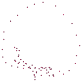
((a)) Dimension reduction result

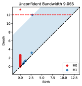
((b)) Persistence diagram with unconfident band

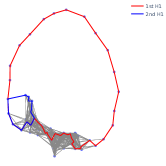
((c)) Longest uncertain H1 representative (Blue) and certain H1 representative (Red)

Figure 1: Dimension reduction results of Tomato dataset by first using PCA to reduce dimension to 10 and then using our PH optimization to reduce to 2.

This selection procedure can be used to assess how well any transformation of point cloud data $X$ preserves topology. In particular, we can compute the bottleneck distance $\epsilon=d_{\mathrm{I}}(H_{k}(X),H_{k}(Y))$, the number of features of $H_{k}(Y)$ with $|d-b|>2\epsilon$ and the number of features of $H_{k}(X)$ with $|d-b|>4\epsilon$. In the context of dimension reduction, it would be desirable to minimize the interleaving distance in order to maximize the number of features we can identify which are in correspondence with features in the original data set. This is the approach we pursue in Section 4.

In table Table 1 we compare several algorithms for dimension reduction on a set of images from the Columbia Object Image Library (COIL-100) [28] taken of a tomato at various angles in a circle which has a single large $H_{1}$ homological feature in the original data. Methods compared include PCA, MDS [23], and ISOMAP [32] with a method based on minimizing the bottleneck distance developed in Section 4, PH, and a hybrid PH + PCA. Because every Vietoris-Rips filtration has a single $H_{0}$ pair with death at $\infty$, at least one $H_{0}$ feature will always be selected. Only PH + PCA allows for the selection of an $H_{1}$ feature. Visualization of each embedding can be found in the appendix, and a more detailed visualization of the PH + PCA embedding can be found in Figure 1.

Method	max $H_{1}$	$\mathrm{d}_{\mathrm{I}}$ $H_{0}$	$\mathrm{d}_{\mathrm{I}}$ $H_{1}$	$H_{0}$	$H_{1}$
PCA	4.854	5.148	10.852	1	0
MDS	5.626	4.782	10.217	1	0
ISOMAP	113.968	1.935	108.623	1	0
PH	7.543	5.295	5.295	1	0
PH + PCA	9.234	4.689	4.532	1	1

Table 1: Selection of topological features. $\max H_{1}$ is the length of the largest $H_{1}$ pair in $Y$. The last two columns indicate the number of features which are in correspondence with the original data in $H_{0}$ and $H_{1}$ via the interleaving.

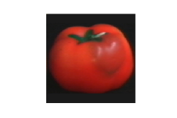
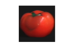
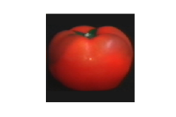
Figure 2: Tomato pictures token from 0, 50, and 100 degree angles. In total, there are 72( = $\frac{360}{5}$) different angles.

3.3 Homological Caveats

Some care must be taken in interpreting the interleaving as presented here. Importantly, the correspondence between persistence pairs of $H_{k}(X)$ and $H_{k}(Y)$ is entirely algebraic; there are not necessarily topological shift maps $f:\mathcal{R}(X;r)\to\mathcal{R}(Y;r+\epsilon)$ and $g:\mathcal{R}(Y;r)\to\mathcal{R}(X;r+\epsilon)$ which induce the interleaving on homology. Even if the interleaving distance between $X$ and $Y$ is zero, there is no guarantee that there is a natural topological map between the two spaces. There are many possible spaces which have identical persistent homology [10], and to maintain some level of geometric interpretability of persistence pairs of $Y$ in terms of the persistence pairs of $X$, it is desirable to incorporate additional constraints onto the embedding $Y$, as is often the case in dimension reduction algorithms.

4 Optimizing Interleaving Distance

We now turn to explicitly optimizing an embedding $Y$ to minimize the interleaving distance to the original data set $X$.

4.1 Optimizing Persistent Homology

Gradient-based optimization techniques can be applied to persistent homology by backpropagating the gradient of a function of the persistence pairs back to the input values of a filtration. This is often done by considering a featurization of the persistence pairs such as algebraic functions of the pairs [17] or persistence landscapes [22, 6], but in our situation, we will use the bottleneck distance $\mathrm{d}_{\mathrm{B}}(\operatorname{dgm}(X),\operatorname{dgm}(Y))$.

Optimization with Vietoris-Rips filtrations is described in detail in [17], which we summarize here. The key is that every simplex addition in the filtration either creates or destroys homology and the corresponding birth or death takes that filtration value. If $f$ is a function of persistence pairs, this allows for the mapping of $\partial f/\partial b$ or $\partial f/\partial d$ to $\partial f/\partial w_{\sigma}$ where $w_{\sigma}$ is the filtration value of the unique simplex $\sigma$. In the case of Vietoris-Rips filtrations, the filtration value of a simplex $(x_{0},\dots,x_{k})$ is the maximum pairwise distance $d_{Y}(x_{i},x_{j})$ where $x_{i},x_{j}$ are vertices in the simplex, so this can then be backpropagated to a gradient $\partial f/\partial d_{Y}(x_{i},x_{j})$. There is a potential issue here which is that a single edge may map to multiple higher-order simplices, but Theorem 4.2 indicates that this is not generally a problem. Finally, if we choose a differentiable metric on $Y$ such as the Euclidean metric, we can backpropagate the gradient to point locations in the embedding.

4.2 Optimizing the Bottleneck Distance

We are interested in optimizing the embedding $Y$ to minimize the interleaving distance via the bottleneck distance $\mathrm{d}_{\mathrm{B}}(\operatorname{dgm}(Y),\operatorname{dgm}(X))$. Because the original data set $X$ is fixed, we have a function $f(\operatorname{dgm}(Y))=\mathrm{d}_{\mathrm{B}}(\operatorname{dgm}(Y),\operatorname{dgm}(X))$ which we can fit into the optimization framework for persistent homology.

First, we recall that the bottleneck distance uses a matching between persistence pairs of $Y$ and $X$ and the diagonal $\Delta$ representing potential zero-length pairs, and that the distance is computed from the maximum-weight matching. This leads to three possibilities.

1. The maximum weight matching occurs between two non-diagonal pairs.

2. The maximum weight matching occurs between a pair in $\operatorname{dgm}(Y)$ and the diagonal in $\operatorname{dgm}(X)$.

3. The maximum weight matching occurs between the diagonal in $\operatorname{dgm}(Y)$ and and a pair in $\operatorname{dgm}(X)$.

The bottleneck distance does not consider matchings between two diagonal points. In the first two cases, it is possible to find a descent direction. In the third case, $Y$ is at a local saddle point of the bottleneck distance.

We will show that under the condition that a single pair attains the maximum-weight matching, we may obtain a descent direction for $\mathrm{d}_{\mathrm{B}}$ with respect to the point locations in $Y$. This is a mild condition observed in practice in our empirical experiments.

Proposition 4.1.

If a single pair $(b,d)$ in the maximum-weight matching of $\operatorname{dgm}(Y)$ and $\operatorname{dgm}(X)$ realizes the bottleneck distance, then the backpropagated $\frac{\partial\mathrm{d}_{\mathrm{B}}}{\partial d(y_{i},y_{j})}$ is non-zero for at most two pairwise distances in $Y$.

Proof.

Because a single pair realizes the distance, it must have non-zero length. In this case, the associated simplex filtration values must map to distinct distances in $Y$. Let $q$ denote the matched point in $\operatorname{dgm}(X)$, so $\mathrm{d}_{\mathrm{B}}(\operatorname{dgm}(Y),\operatorname{dgm}(X))=\|(b,d)-q\|_{\infty}$, one or both distances may admit a non-zero gradient. ∎

Theorem 4.2.

If a single pair in $\operatorname{dgm}(Y)$ realizes the bottleneck distance, then $\mathrm{d}_{\mathrm{B}}(\operatorname{dgm}(Y),\operatorname{dgm}(X))$ admits a descent direction on the point embedding $Y$.

Proof.

From Proposition 4.1, there are at most two pairwise distances which have a non-zero backpropagated gradient. Let these distances be $d_{Y}(y_{0},y_{1})$ and $d_{Y}(y_{2},y_{3})$. If the points $y_{0},y_{1},y_{2},y_{3}$ are distinct, then we can simply backpropagate the gradient to each point location.

One point might possibly participate in both distances – if two points are redundant, then the distances are not distinct. In this case, let us have $b=d_{Y}(y_{0},y_{1})$ and $d=d_{Y}(y_{1},y_{2})$. In this case, we can take a step in the directions $\frac{\partial\mathrm{d}_{\mathrm{B}}}{\partial y_{0}}=\frac{\partial\mathrm{d}_{\mathrm{B}}}{\partial b}\frac{\partial b}{\partial y_{0}}$, $\frac{\partial\mathrm{d}_{\mathrm{B}}}{\partial y_{2}}=\frac{\partial\mathrm{d}_{\mathrm{B}}}{\partial d}\frac{\partial d}{\partial y_{2}}$, and leave $y_{1}$ unchanged. Because $\frac{\partial d_{Y}(y_{0},y_{1})}{\partial y_{0}}$ and $\frac{\partial d_{Y}(y_{0},y_{1})}{\partial y_{1}}$ are non-zero, and at least one of $\frac{\partial\mathrm{d}_{\mathrm{B}}}{\partial d}$ or $\frac{\partial\mathrm{d}_{\mathrm{B}}}{\partial d}$ is non-zero, this step direction will decrease the bottleneck distance. ∎

Proposition 4.3.

$\nabla_{Y}\mathrm{d}_{\mathrm{B}}(\operatorname{dgm}(Y),\operatorname{dgm}(X))$ admits a generalized subdifferential.

Proof.

Any persistence pair in $\operatorname{dgm}(Y)$ that does not participate in the bottleneck matching can be perturbed without affecting the bottleneck distance. ∎

Proposition 4.3 implies that we have great freedom to perturb the embedding $Y$ while minimizing the bottleneck distance. In the third case above, when the diagonal of $\operatorname{dgm}(Y)$ is involved in the maximum weight matching, we have the freedom to perturb $Y$ in any direction. This allows for easy optimization of the bottleneck distance in conjunction with a secondary objective.

5 Experiments

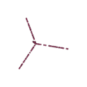
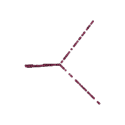
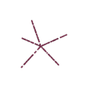
Figure 3: Dimension reduction results of 5-Tendril left to right: PCA, MDS and PH

In this section, we will introduce the experiments and results using our dimension reduction method. For convenience, we will call our method PH optimization as it based on persistent homology.

We implement a form of projection pursuit [16] which seeks to find a linear projection $P$ which minimizes the bottleneck distance between $X$ and $Y=XP$. We add the orthogonality constraint to the optimization candidate space (also called Stiefel manifold) and the optimization gradient descent algorithm will use the Cayley transform introduced in [35].

In our dimension reduction method, since optimization requires repeated computation of persistent homology, controlling the number of points is crucial. In an effort to obtain a sample with close persistent homology, we use a greedy strategy based on minimizing the Hausdorff distance from the sample to the full point cloud. However, recall that Corollary 2.8 requires Gromov–Hausdorff distance which requires solving quadratic assignment problem. We will bound the Gromov–Hausdorff distance by Hausdorff returned from the greedy sampling algorithm.

Our procedure is implemented in Pytorch, which supports automatic differentiation without explicitly passing gradients once we have defined two layers: a Vietoris-Rips layer and a bottleneck distance layer. The Rips layer based on BATS will compute persistent homology of a Rips filtration and find the inverse map described in Section 4.1. The bottleneck distance layer is supported by Hera [21], which can efficiently find the matching for bottleneck distance.

5.1 5-Tendril

We generate a data set, 5-Tendril consisting of 500 points in 5 dimensions sampled along 5 tendrils, each of which consists of 50 randomly generated points on a canonical basis vector $e_{i}$ of Euclidean space. Here, our PH optimization method will first sample 100 points and then optimize the bottleneck distance on H0 persistent diagram. We perform 3 different dimension reduction algorithms: PCA, MDS and PH optimization. In Figure 3, the results show that PCA and MDS can only see 3 branches, while PH optimization can see 5.

5.2 Orthogonal Cycle

We generate a data set of 500 samples in 5 dimensions with $\binom{5}{2}=10$ cycles, each of which consists of 50 points and lies in a 2-dimensional plane spanned by two canonical bases $e_{i}$ and $e_{j}$ with center $e_{i}$ + $e_{j}$ and radius one. For speedup, our PH optimization method samples 200 points and then optimizes bottleneck distance on $H_{1}$.

Since the dataset consists of cycles in orthogonal planes and our PH optimization method will also purse an orthonormal projection, there is no way to find a projection that can show and divide all cycles apart within the orthogonality constraint. In Figure 4, we show the dimension reduction results with 4 different methods: PCA will lead to a tangle where cycles cross with each other, and if without labels, one cannot tell how many cycles exist in this plot; ISOMAP will provide us a five-star with half of orthogonal cycles missed, but without labels, it is hard to determine if there are cycles exists; MDS can provide a 5-ring, but some of are not comprised of a single orthogonal cycle, for example, the yellow orthogonal cycle lies on two rings; our PH method can provide 3 cycles and the three straight lines between can indicate the collapse of orthogonal structure in the projection.

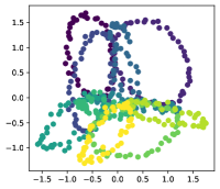
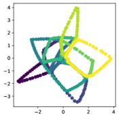
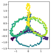
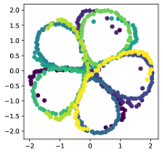
Figure 4: Dimension Reduction Results of Orthogonal cycles data set. Left to right: PCA, MDS, ISOMAP and PH

5.3 COIL-100

The Columbia Object Image Library (COIL-100) [28] dataset contains 7200 colorful images of 100 objects, where each object has 72 $128\times 128$ images with 3 color channels taken at pose intervals of 5 degrees. We pick the tomato dataset (see Figure 2) with shape $72\times 49152(=128*128*3)$ from COIL-100 and perform our PH optimization algorithm on both $H_{1}$ and $H_{0}$ persistent diagrams. Although the number of points is only 72, the high feature dimension makes the direct running of our procedure on Pytorch prohibitive due to the memory issue of Cayley transform. To solve the problem, we devise two procedures: a) Optimizing the projection directly using the Cayley transform to handle orthogonality; b) first we perform PCA on the tomato dataset to reduce dimension to 10 and then keep reducing the dimension to 2 by our Pytorch PH optimization algorithm, denoted by PH+PCA.

We include visualization of the results using methods PH, PH+PCA, PCA, ISOMAP, MDS into the Appendix and show the result of PH+PCA in Figure 1. In Figure 1a), we can see that the 72 points in $\mathbb{R}^{2}$ constitute a great circle, which demonstrate that the dataset consists of pictures taken at 360 degrees at pose interval 5 around the tomato. In Figure 1b), we draw the persistence diagram of the projected data set and a unconfident band with width 9.065, which is the twice of bottleneck distance between the original and projected tomato dataset. By the discussion in Section 3, there is only one H1 class in the projected data that we can ensure also exists in the original one. In Figure 1c), we then draw the certain H1 representative in red and the longest uncertain H1 representative in blue.

5.4 Natural Image Patches

Natural image patches are a well-studied data set with interesting topological structures at various densities [4]. We follow the data processing procedure of [24] to sample $3\times 3$ patches from the van Hateren natural images database [33]. We further refine a sub-sample of 50,000 patches using the co-density estimator of [11] with $k=5,p=40\%$ to obtain a data set of 20,000 patches which resembles the “three-circle” model of [11].

In Figure 5 we apply our procedure to two initial projections. In both cases, we use a greedy subsampling of 100 points in the data which contains 5 robust $H_{1}$ pairs, agreeing with the three-circle model. We first initialize the projection with the first two principal components of the data and then refine by optimizing the bottleneck distance on $H_{1}$ pairs. The initial projection onto principal components displays a clear “primary circle,” with the two secondary circles projecting onto two chords. Our procedure decreases the $H_{1}$ bottleneck distance on the 100 sampled points from $5.6$ to $4.7$ but there is minimal visual difference between the two projections, indicating that the initialization was near a local optimum.

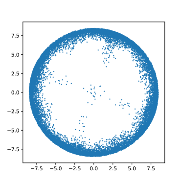
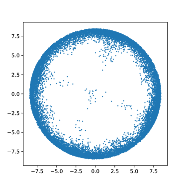
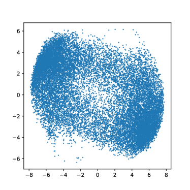
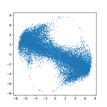
Figure 5: Projections of a $3\times 3$ image patch data set. Top row, left to right: principal component embedding, and further refinement from minimizing $H_{1}$ bottleneck distance. Bottom row: random projection and further refinement from minimizing $H_{1}$ bottleneck distance.

The second row of Figure 5 starts with a random projection into two dimensions. We again optimize to minimize the bottleneck distance on the $H_{1}$ pairs, and decrease the bottleneck distance on the sampled points from $7.9$ to $3.7$. In this case, there is a noticeable visual difference between the two projections. In the first projection, a noisy projection of the primary circle is visible, and in the second projection, we see a clear visualization of one of the two secondary circles, with the primary circle and other secondary circle collapsed to a chord.

In both these experiments, our $H_{1}$ bottleneck distance bounds do not allow us to confidently select any features in the visualization. As with the orthogonal cycle data, the reason is fundamental: the three circle model embeds into a Klein bottle [4], and any projection to fewer than 4-dimensions (necessary to embed the Klein bottle) will result in spurious intersections of at least two of the three circles. Despite these limitations, our method is still able to present a subset of the important $H_{1}$ features of this data.

6 Discussion

In this paper, we propose the use of the interleaving distance in dimensionality reduction. We show that this distance can be used to identify topological features in correspondence between a full data set $X$ and a low dimensional embedding $Y$ using any dimension reduction procedure. We also demonstrate how optimization of the equivalent bottleneck distance can increase the significance of important topologcial features in $X$ in the embedding $Y$.

We incorporate bottleneck distance optimization into projection pursuit and find that our method can preserve topological information when projecting from high dimensional spaces to two dimensions for visualization. We find in several cases, our method will focus on visualizing a subset of the important topological structures as orthogonality of subspaces in the full data set prohibit the visualization of all structures using a single projection.

Our method could be combined with other optimization objectives such as the maximization of variance in the projection as in PCA. One limitation of our method is that the bottleneck distance is non-smooth and has many local minima. Hybrid schemes which combine bottleneck distance optimization with other objectives may generally help with optimization.

One direction of future work that could help improve the ability to detect if topological features in embeddings has correspondence with the original data set would be to develop interleaving techniques based on non-linear shift maps. Because the interleaving distance focuses on the worst possible distortion between persistent homologies, a more fine-grained analysis may reveal that more information is preserved in practice.

Appendix A Appendix

A.1 Additional Dimension Reduction Results

Method	Bottleneck Distances (B0, B1)	Dimension reduced data
PH + PCA	4.689, 4.532
PH	5.295, 12.661
PCA	5.148, 10.852
ISOMAP	1.935, 108.623
MDS	4.782, 10.217

Table 2: Dimension Reduction Results of tomato dataset from COIL-100

References

- [1] Bubenik, P., and Scott, J. A. Categorification of Persistent Homology. Discrete & Computational Geometry 51, 3 (Apr. 2014), 600–627.
- [2] Carlsson, G. Topological pattern recognition for point cloud data. Acta Numerica 23 (May 2014), 289–368.
- [3] Carlsson, G., and de Silva, V. Zigzag Persistence. Foundations of Computational Mathematics 10, 4 (Aug. 2010), 367–405.
- [4] Carlsson, G., Ishkhanov, T., de Silva, V., and Zomorodian, A. On the Local Behavior of Spaces of Natural Images. International Journal of Computer Vision 76, 1 (Jan. 2008), 1–12.
- [5] Carriere, M., Chazal, F., Glisse, M., Ike, Y., Kannan, H., and Umeda, Y. Optimizing persistent homology based functions. In Proceedings of the 38th International Conference on Machine Learning (July 2021), PMLR, pp. 1294–1303.
- [6] Carriere, M., Chazal, F., Ike, Y., Lacombe, T., Royer, M., and Umeda, Y. PersLay: A Neural Network Layer for Persistence Diagrams and New Graph Topological Signatures. In Proceedings of the Twenty Third International Conference on Artificial Intelligence and Statistics (June 2020), PMLR, pp. 2786–2796.
- [7] Chazal, F., Cohen-Steiner, D., Glisse, M., Guibas, L. J., and Oudot, S. Y. Proximity of persistence modules and their diagrams. In Proceedings of the 25th Annual Symposium on Computational Geometry - SCG ’09 (Aarhus, Denmark, 2009), ACM Press, p. 237.
- [8] Chazal, F., Cohen-Steiner, D., Guibas, L. J., Mémoli, F., and Oudot, S. Y. Gromov-Hausdorff Stable Signatures for Shapes using Persistence. In Computer Graphics Forum (2009), vol. 28, Wiley Online Library, pp. 1393–1403.
- [9] Cohen-Steiner, D., Edelsbrunner, H., and Harer, J. Stability of Persistence Diagrams. Discrete & Computational Geometry 37, 1 (Jan. 2007), 103–120.
- [10] Curry, J. The Fiber of the Persistence Map. Journal of Applied and Computational Topology 2, 3 (2018), 301–321.
- [11] de Silva, V., and Carlsson, G. Topological estimation using witness complexes. In Proc. Sympos. Point-Based Graphics (June 2004).
- [12] de Silva, V., Morozov, D., and Vejdemo-Johansson, M. Persistent Cohomology and Circular Coordinates. Discrete & Computational Geometry 45, 4 (June 2011), 737–759.
- [13] Doraiswamy, H., Tierny, J., Silva, P. J. S., Nonato, L. G., and Silva, C. TopoMap: A 0-dimensional Homology Preserving Projection of High-Dimensional Data. IEEE Transactions on Visualization and Computer Graphics 27, 2 (Feb. 2021), 561–571.
- [14] Edelsbrunner, Letscher, and Zomorodian. Topological Persistence and Simplification. Discrete & Computational Geometry 28, 4 (Nov. 2002), 511–533.
- [15] Fasy, B. T., Lecci, F., Rinaldo, A., Wasserman, L., Balakrishnan, S., and Singh, A. Confidence Sets for Persistence Diagrams. The Annals of Statistics 42, 6 (2014), 2301–2339.
- [16] Friedman, J. H., and Tukey, J. W. A Projection Pursuit Algorithm for Exploratory Data Analysis. IEEE Transactions on Computers C-23, 9 (Sept. 1974), 881–890.
- [17] Gabrielsson, R. B., Nelson, B. J., Dwaraknath, A., and Skraba, P. A Topology Layer for Machine Learning. In International Conference on Artificial Intelligence and Statistics (June 2020), PMLR, pp. 1553–1563.
- [18] Hatcher, A. Algebraic Topology. Cambridge University Press, Cambridge ; New York, 2002.
- [19] Hofer, C., Graf, F., Rieck, B., Niethammer, M., and Kwitt, R. Graph Filtration Learning. In Proceedings of the 37th International Conference on Machine Learning (Nov. 2020), PMLR, pp. 4314–4323.
- [20] Kachan, O. Persistent Homology-based Projection Pursuit. In 2020 IEEE/CVF Conference on Computer Vision and Pattern Recognition Workshops (CVPRW) (Seattle, WA, USA, June 2020), IEEE, pp. 3744–3751.
- [21] Kerber, M., Morozov, D., and Nigmetov, A. Geometry helps to compare persistence diagrams. Journal of Experimental Algorithmics (JEA) 22 (2017), 1–20.
- [22] Kim, K., Zaheer, M., Chazal, F., Kim, J., Kim, J. S., and Wasserman, L. PLLay: Efficient Topological Layer based on Persistence Landscapes. In Advances in Neural Information Processing Systems (2020), vol. 33, p. 13.
- [23] Kruskal, J. B. Multidimensional scaling by optimizing goodness of fit to a nonmetric hypothesis. Psychometrika 29, 1 (Mar. 1964), 1–27.
- [24] Lee, A. B., Pedersen, K. S., and Mumford, D. B. The Nonlinear Statistics of High-Contrast Patches in Natural Images. International Journal of Computer Vision 54, 1-3 (2003), 83–103.
- [25] Lesnick, M. The Theory of the Interleaving Distance on Multidimensional Persistence Modules. Foundations of Computational Mathematics 15, 3 (June 2015), 613–650.
- [26] Leygonie, J., Oudot, S., and Tillmann, U. A Framework for Differential Calculus on Persistence Barcodes. Foundations of Computational Mathematics (July 2021).
- [27] Moor, M., Horn, M., Rieck, B., and Borgwardt, K. Topological Autoencoders. In Proceedings of the 37th International Conference on Machine Learning (Nov. 2020), PMLR, pp. 7045–7054.
- [28] Nene, S. A., Nayar, S. K., and Murase, H. object image library (coil-100. Tech. rep., 1996.
- [29] Poulenard, A., Skraba, P., and Ovsjanikov, M. Topological Function Optimization for Continuous Shape Matching. Computer Graphics Forum 37, 5 (Aug. 2018), 13–25.
- [30] Rieck, B., and Leitte, H. Persistent Homology for the Evaluation of Dimensionality Reduction Schemes. Computer Graphics Forum 34, 3 (2015), 431–440.
- [31] Rieck, B., and Leitte, H. Agreement Analysis of Quality Measures for Dimensionality Reduction. In Topological Methods in Data Analysis and Visualization IV, H. Carr, C. Garth, and T. Weinkauf, Eds. Springer International Publishing, Cham, 2017, pp. 103–117.
- [32] Tenenbaum, J. B., de Silva, V., and Langford, J. C. A Global Geometric Framework for Nonlinear Dimensionality Reduction. Science 290, 5500 (Dec. 2000), 2319–2323.
- [33] van Hateren, J. H., and van der Schaaf, A. Independent component filters of natural images compared with simple cells in primary visual cortex. Proceedings. Biological Sciences 265, 1394 (Mar. 1998), 359–366.
- [34] Wagner, A., Solomon, E., and Bendich, P. Improving Metric Dimensionality Reduction with Distributed Topology. arXiv:2106.07613 [cs, math] (Sept. 2021).
- [35] Wen, Z., and Yin, W. A feasible method for optimization with orthogonality constraints. Mathematical Programming 142 (2013), 397–434.
- [36] Yan, L., Zhao, Y., Rosen, P., Scheidegger, C., and Wang, B. Homology-Preserving Dimensionality Reduction via Manifold Landmarking and Tearing. arXiv:1806.08460 [cs] (June 2018).
- [37] Yu, B., and You, K. Shape-Preserving Dimensionality Reduction : An Algorithm and Measures of Topological Equivalence. arXiv:2106.02096 [cs, stat] (June 2021).
- [38] Zomorodian, A., and Carlsson, G. Computing Persistent Homology. Discrete & Computational Geometry 33, 2 (Feb. 2005), 249–274.