Magnetar XTE J1810$-$197: Spectro-temporal Evolution of Average Radio Emission

Abstract

We present the long-term spectro-temporal evolution of the average radio emission properties of the magnetar XTE J1810$-$197 (PSR J1809$-$1943) following its most recent outburst in late 2018. We report the results from two and a half years of monitoring campaign with the upgraded Giant Metrewave Radio Telescope carried out over the frequency range of 300$-$1450 MHz. Our observations show intriguing time variability in the average profile width, flux density, spectral index and the broadband spectral shape. While the average profile width appears to gradually decrease at later epochs, the flux density shows multiple episodes of radio re-brightening over the course of our monitoring. Our systematic monitoring observations reveal that the radio spectrum has steepened over time, resulting in evolution from a magnetar-like to a more pulsar-like spectrum. A more detailed analysis reveals that the radio spectrum has a turnover, and this turnover shifts towards lower frequencies with time. We present the details of our analysis leading to these results, and discuss our findings in the context of magnetar radio emission mechanisms as well as potential manifestations of the intervening medium. We also briefly discuss whether an evolving spectral turnover could be an ubiquitous property of radio magnetars.

1 Introduction

Magnetars are highly magnetized ($10^{13}-10^{15}$ G) neutron stars having long spin periods (1.3 $-$ 12 s). They are powered by the decay of their internal magnetic field rather than the rotational kinetic energy (Duncan & Thompson, 1992) and some of them show radio emission after a high-energy burst or flare (e.g. Camilo et al., 2006). Currently, five magnetars are known to exhibit transient periodic radio emission, and another one produces isolated radio bursts (see McGill magnetar catalog; Olausen & Kaspi, 2014). They typically display time variability in many characteristics like radio flux density, spectra and integrated profile shapes. The radio emission typically has a flat spectrum. This has enabled the study of the radio emission at radio frequencies as high as 353 GHz for some of the radio-loud magnetars (Torne et al., 2022). The very high frequency observations indicate that the radio spectrum has a high frequency turn-up. However, the low frequency end of the radio spectrum has not been explored through regular monitoring observations in the past.

XTE J1810$-$197 was discovered during an outburst in 2004 (Ibrahim et al., 2004) and was the first radio-loud magnetar (Camilo et al., 2006). Following the onset, the radio pulsations lasted for nearly three years before becoming undetectable around 2008 (Camilo et al., 2016). During the radio-loud episode, the magnetar showed time variable flux density, pulse profile and spectral index (Camilo et al., 2007a, b; Lazaridis et al., 2008). The radio flux density declined initially. Then it seemed to vary around a steady value before the radio pulsations stopped abruptly (Camilo et al., 2016).

The current activity began in late 2018 with an intense episode in radio and X-ray (Lyne et al., 2018; Gotthelf et al., 2018). Radio pulsations were soon detected at a very broad range of radio frequencies and follow-up observations have been continuing since then (Joshi et al., 2018; Trushkin et al., 2019; Dai et al., 2019; Torne et al., 2020). Similar to the last outburst, the magnetar has shown variations in profile shape, flux density as well as single-pulse properties (Dai et al., 2019; Levin et al., 2019; Maan et al., 2019; Caleb et al., 2021). In our previous paper (Maan et al., 2019), we primarily reported on the single-pulse properties, along with the low-frequency radio flux density and spectrum of the magnetar close to the outburst. As mentioned earlier, a broad-band radio spectrum is crucial in order to understand the emission mechanism. Given most of the current monitoring campaigns observe the magnetar at frequencies higher than 1 GHz, our campaign has made use of the upgraded Giant Metrewave Radio Telescope (GMRT; Gupta et al., 2017) to cover a frequency range of 300$-$1450 MHz.

In this paper, we report on the temporal evolution of the pulsed flux density, spectral index as well as the average profile width from our monitoring campaign. We describe the observations in Section 2, results and analysis in Sections 3 and 4, and discuss the implications in Section 5

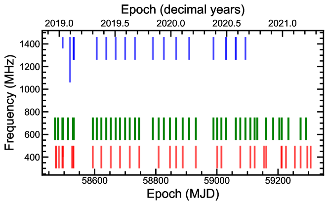
Figure 1: A summary of the observations presented in this paper. The individual vertical bars indicate the frequency range covered by an observation at a particular epoch. The red, green and blue colored bars represent bands 3 (300$-$500 MHz), 4 (550$-$750 MHz) and 5 (typically 1260$-$1460 MHz) of GMRT, and the same color convention has been followed in the rest of the paper. The band 5 observations at the first two epochs utilized bandwidths of 100 and 400 MHz, respectively, and 200 MHz at all the other epochs.

2 Observations and data reduction

After successful detection and follow-up of the magnetar XTE J1810$-$197 at a number of epochs in late 2018 and early 2019 (Joshi et al., 2018; Maan et al., 2019) using the Director’s Discretionary Time allocations, we started a low-frequency monitoring campaign on this source with the GMRT. The monitoring observations utilized bands 3, 4 and 5 of the GMRT with typical center frequencies of 400, 650 and 1360 MHz, respectively, and 200 MHz bandwidths at each of the bands. Depending on the spectral and temporal evolution of the magnetar’s flux density, the observations were conducted in a number of configurations: simultaneous observations in two or three bands at a few epochs by combining GMRT antennae in two or three sub-arrays, near-simultaneous observations in two of the bands by observing in one band after the other, or just single band observations. The near-simultaneous observations always included band 4 as one of the two bands. After September 2020, the monitoring observations were limited to bands 3 and 4. Figure 1 shows the cadence and a summary of all the observations presented in this paper.

The observation on MJD 58495 was conducted simultaneously in bands 3, 4 and 5, and the bandwidth in each of the band was limited to 100 MHz in this configuration. However, only band 5 data could be used from this observation due to severe contamination by radio frequency interference (RFI) in the other two bands. As apparent in Figure 1, the band 5 observation on MJD 58519 employed 400 MHz bandwidth. A bandwidth of 200 MHz was utilized in all the subsequent band 5 observations, many of which were conducted in an observing mode that facilitated simultaneous dual-band observations and limited the bandwidth to 200 MHz. Initially, the observing setup constituted 8192 channels and 0.328 or 0.655 ms time resolution in band 3, and 4096 channels and 0.164 ms sampling time in bands 4 and 5. Since November 2020, we used an observing mode wherein the data are coherently dedispersed at a dispersion measure (DM) of 178.85  pc cm^-3 in real time and then recorded to the disk with 1024 frequency sub-bands, and sampling times of 0.164 and 0.081 ms in bands 3 and 4, respectively.

The recorded data for all the bands are processed through a series of data reduction steps. For the observations prior to November 2020, we use SIGPROC’s dedisperse to sub-band the data to 1024 channels wherein the data within each sub-band is dedispersed using a DM of 178.85  pc cm^-3. As mentioned above, observations after November 2020 were already recorded with 1024 coherently dedispersed sub-bands. The data from the individual epochs are then subjected to size reduction by down-sampling from 16 bits to 8 bits per sample using digifil, and RFI excision using RFIClean (Maan et al., 2021) and rfifind from the pulsar search and analysis toolkit PRESTO (Ransom et al., 2002). The resultant data are folded using prepfold from PRESTO and the timing parameters from Levin et al. (2019), with 1024 bins, 128 sub-bands and typically 64 sub-intervals. This PRESTO utility outputs partially folded data along with the several pieces of information, including the period and DM values which maximize the average profile signal-to-noise ratio (S/N), in files with extensions pfd, which we refer to as pfd-files here onwards.

3 Analysis and Results: Flux density, spectral index, profile width and their temporal evolution

3.1 Calibration procedure

In a number of our observing sessions, we had carried out scans on flux calibrators (3C286 and 3C48) as well as a few degrees away from them. Using these on-source and off-source calibrator observations, we estimated the system equivalent flux density (hereafter SEFD, defined as the ratio of the system temperature and the gain, T_sys/G) per GMRT dish as a function of frequency and fitted a polynomial to these measurements. For band 4, the estimated SEFD compares well with the polynomial fits for the sensitivity used in the GMRT exposure time calculator (ETC). For band 5, only a few calibrator scans were available and some of these were heavily contaminated by RFI. Nevertheless, we could estimate the SEFD for band 5 using one set of calibrator scans, and it was found to be slightly offset from the polynomial fit used in ETC. For band 3, the SEFD could be estimated using calibrator scans at several epochs, however, the SEFD measurements show a large spread around the mean value.

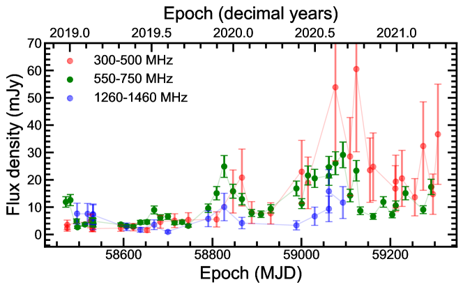
Figure 2: Period averaged flux densities as a function of epoch, measured in the individual bands 3 (300$-$500 MHz), 4 (550$-$750 MHz) and 5 (1260$-$1460 MHz).

We read the partially folded data from the pfd-files in python using the class pfd provided in PRESTO, and re-fold these using the best period and DM values suggested by prepfold. Despite the RFI excision using RFIClean as well as rfifind, some faint RFI becomes visible only in the partially folded data, which primarily appears in the form of baseline variations. It is important to get rid of or correct for these baseline variations to correctly estimate the flux density using the radiometer equation (Lorimer & Kramer, 2004). However, the long period of the magnetar also does not help in averaging out these variations. To remedy the situation, the off-pulse regions of the profiles from the sub-intervals and sub-bands are used to estimate robust statistics and then subjected to a threshold-based identification of outliers. Additionally, 12.5% of the sub-bands on either side of the band, as well as the sub-bands in the frequency range 355$-$385 MHz (which is often contaminated by the signals from the MUOS satellites), are also considered as outliers. For severely RFI contaminated data, the sub-interval profiles are also inspected by eye to identify the ones with visibly contaminated baselines. The outlier sub-intervals and sub-bands thus identified are excluded from any further processing. These data are then averaged fully over time and to a pre-specified number of final sub-bands, which is typically 4 for band 4, 4 or 2 for band 3 and just 1 (i.e., averaged over the full bandwidth) for band 5. The off-pulse regions of the sub-banded profiles were also fitted by a 3^rd order (9^th order for profiles with S/N$>$500) polynomial to get rid of any remaining baseline variations. These sub-banded and baseline-corrected average profiles are then flux calibrated by estimating the mean and standard deviation in the off-pulse region and using the radiometer equation with the SEFD estimates described above. The observing time and bandwidth is appropriately accounted for the sub-intervals and sub-bands/channels that are identified as outliers by rfifind as well as in the above post-processing. The frequency-dependent sky temperature towards the source is estimated using the skytempy package, which is based on the reprocessing of the Haslam et al. (1982) 408 MHz map by Remazeilles et al. (2015). Assuming receiver temperatures of 85, 87 and 62 K at the centers of the bands 3, 4 and 5, respectively, a constant gain throughout the bands and the sky temperature estimates from above, the SEFD is re-estimated towards the source before using in the radiometer equation. Furthermore, we assume that the signals from different antennae in a sub-array are added fully coherently, i.e., the gain of a sub-array is linearly proportional to the number of antennae.

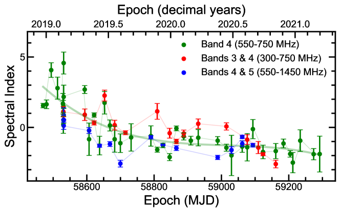
Figure 3: Power-law spectral indices estimated using the period averaged flux densities measured in band 4, bands 3 & 4, and bands 4 & 5. The light-green colored thick, continuous curve shows a $3^{rd}$-order polynomial fit to the band 4 estimates, only to demonstrate the temporal evolution of the spectral indices and guide the eye.

3.2 Flux density

By integrating the area under these flux-calibrated, sub-banded profiles, we estimate the period-averaged flux densities for each of the sub-bands. The corresponding uncertainties are estimated by assuming 5% and 10% uncertainties in SEFD and the system temperature, respectively. The period-averaged flux density over the entire band is then estimated by averaging the corresponding sub-band estimates. The flux density of the magnetar measured in the three bands is shown as a function of epoch in Figure 2.

We note here that there are primarily three factors which could have affected our flux density measurements. First, as mentioned earlier, we have assumed that the signals from different antennae in a sub-array are added fully coherently. In practice, ionospheric or weather conditions might introduce disturbances in an otherwise coherently phased array. Specifically at low radio frequencies, a full coherence might also not be always achievable. Any such deviation from a fully coherent addition would have resulted in an additional systematic uncertainty.

Second, as XTE J1810$-$197 is a long period pulsar, any low-level baseline variations in the off-pulse region might result in slightly over-estimated standard deviation measurements, and hence, under-estimated flux densities. From all the scrutiny and care taken in excising RFI and baseline correction mentioned in the previous sub-section as well as visual inspection of profiles, we expect this issue to have affected our measurements only at a few epochs.

Third, the large spread in the SEFD measurement at band 3 implies a large uncertainty in our band 3 flux density measurements. The band 5 SEFD was estimated using calibrator scans at only one epoch and it was found to be offset from that used in ETC by about 20%. For these reasons, we have assumed the uncertainties of our band 3 and band 5 flux density measurements to be 50%. We note that our band 5 flux density measurements are largely consistent with those measured using the Jodrell bank telescope at similar epochs (Caleb et al., 2021).

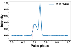
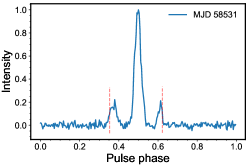
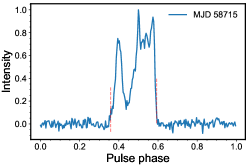
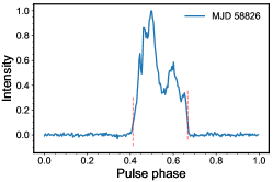
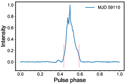
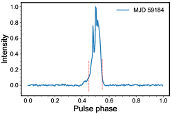
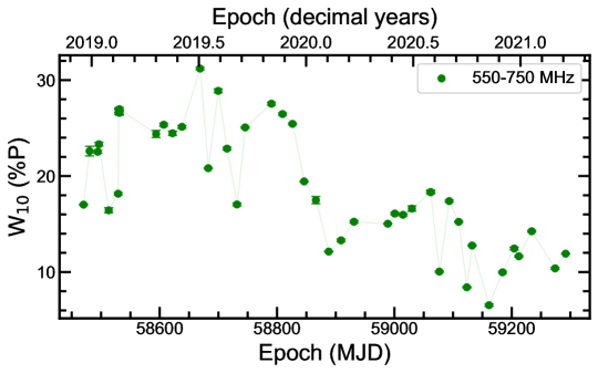
Figure 4: The panels (a) to (f) show 550$-$750 MHz (band 4) average profiles at six different epochs with their peak intensities normalized to 1. The dashed, red-colored lines in these panels mark the 10% crossings in the average profiles at the leading as well as the trailing edges, which are used to estimate $W_{10}$. The lower panel (g) displays the $W_{10}$ measured as a percentage of the pulse period for the 550$-$750 MHz average profiles, as a function of epoch.

3.3 Spectral index

The large fractional bandwidths in band 3 and band 4 enable us to estimate the in-band spectral indices. At a given frequency $\nu$, assuming the flux density, $S_{\nu}\propto\nu^{\alpha}$, we measure the spectral index $\alpha$ by fitting a straight line in the $\log S_{\nu}-\log\nu$ plane. The temporal evolution of the in-band spectral indices measured using band 4 observations is shown in Figure 3 (light green points). A general decrease in the spectral index with time is apparent. Due to poor detection significance at several epochs and contamination by RFI or baseline variations at several other epochs, the in-band spectral indices could not be measured reliably using the band-3 data.

As mentioned in Section 2, a few of our observations were simultaneous in multiple bands, and several others were near-simultaneous either in bands 3 and 4 or in bands 4 and 5. The near-simultaneous observations in two bands were typically separated by nearly 2 hours. We can use these simultaneous as well as the near-simultaneous observations to estimate the spectral indices over wider frequency ranges, assuming the timescale of the intrinsic flux density variations of the magnetar is much longer than 2 hours. The spectral indices measured using bands 3 and 4, and 4 and 5, covering frequency ranges of 300$-$750 MHz and 550$-$1450 MHz, are shown in Figure 3 by red and blue colored points, respectively. As with the in-band spectral indices obtained from band$-$4, these inter-band spectral indices also exhibit a general decreasing trend with time.

3.4 Profile width

The average radio profile of XTE J1810$-$197 changes rapidly with varying number of components and total shape changes from one epoch to the other. An example of this behavior can be seen from the average profiles obtained from our band 4 observations at six different epochs that are shown in Figure 4 to 4 (also see Figure 1 in Caleb et al., 2021). To obtain a reasonable estimate of the pulse-width that can be related to the underlying emission beam, we estimate the positions on the leading as well as the trailing edge where the intensity crosses the 10% of the observed maximum in the profile. In Figure 4 to 4, these crossings are shown using vertical dashed lines in red color. Using these, we estimate the average profile width at the 10% level, $W_{10}$. The profile width thus estimated for all the band 4 profiles which exhibited a peak S/N of more than 25 is shown as a function of epoch in Figure 4. While there are significant epoch-to-epoch variations in the profile width, it is apparent that $W_{10}$ remains about 25% of the magnetar’s spin period up to MJD 58800 or so, and then shows a gradual decrease as a function of time.

We note that the above approach might not take into account very faint leading or trailing components in the profile. Figure 4 represents one such example where the peak of a faint pre-cursor component reaches only a few percent of the maximum in the profile. From manual inspection of the average profiles, we could identify only four other epochs where the average profile exhibits very faint (even fainter than the example in Figure 4) pre-cursor or post-cursor components which are not accounted in $W_{10}$ estimates. We believe that such occasional unaccounted components do not alter the long-term behavior of the profile width apparent in Figure 4.

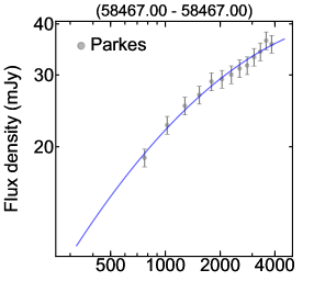
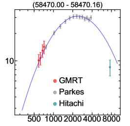
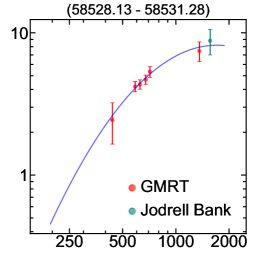
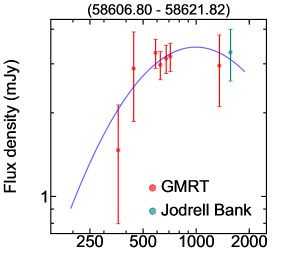
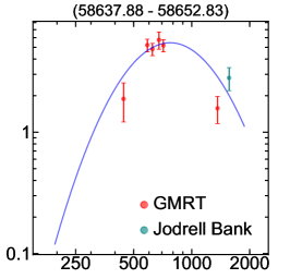
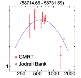
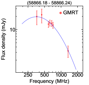
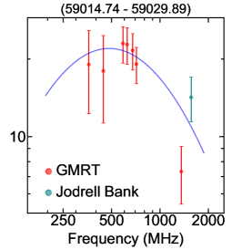
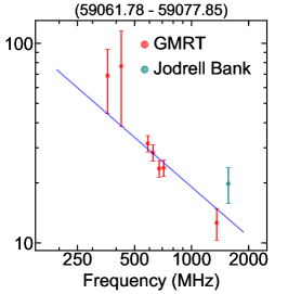
Figure 5: Broadband spectra constructed using multi-band, multi-epoch and multi-telescope measurement are shown at nine different epochs (GMRT measurements are from this work, and the Parkes, Hitachi and Jodrell Bank measurements are from Dai et al. (2019), Eie et al. (2021) and Caleb et al. (2021), respectively). Several of these spectra show clear evidence for a turnover. Also shown are the fits to these spectra, assuming a log-parabola shape of the spectrum.

4 A temporally evolving, turnover in the spectrum?

From the spectral indices shown in Figure 3, it is evident that the magnetar’s radio spectrum has gradually evolved from inverted spectrum closer to the onset of the outburst to as steep as the normal pulsar population at later epochs. However, Figure 3 also indicates that the overall spectrum in the lower frequency range (300$-$750 MHz) is flatter compared to the 550$-$750 MHz range, while that in the higher frequency range (550$-$1450 MHz) is steeper. This trend of spectral indices measured from the lower and higher frequency ranges encompassing those measured from only band 4 continues till about MJD 59000$-$59050, beyond which the spectral indices measured from all the three frequency ranges seem to follow closely.

The above behavior could potentially be explained by a turnover in the spectrum with a peak-frequency that evolves downward with time. To test this hypothesis, we tried to construct broadband spectra at different epochs using our own observations as well as those available from the literature, and fit a spectral shape with a turnover. From our own observations, we consider combining our near-simultaneous observations in bands 3 and 4, and those in bands 4 and 5, to construct a broadband spectrum covering the frequency range 300$-$1450 MHz. These two sets of observations were separated by typically 15 days. As the magnetar exhibits rapid flux density variations, combining observations from different epochs might provide an incorrect representation of the overall spectrum. As band 4 was common in both the sets of observations, we use the measured band-4 flux density to gauge if the flux density has evolved or not, and combine only those sets where the band-4 flux density is relatively unchanged. This approach resulted in broadband spectra at seven epochs.

From the literature, we looked for the flux density measurements available during or at nearby epochs for which we could construct the above described broadband spectra or independent wide-band measurements. We have used published results from Parkes wide-band observations at two epochs (December 15 and 18, 2018; Dai et al., 2019), 7.6 GHz measurement from the Hitachi radio telescope at one epoch (Eie et al., 2021), and Jodrell Bank L-band observations at 6 epochs (Caleb et al., 2021). Wherever the uncertainties were less than 5% or not available at all, we assumed a uniform 5% uncertainty on the published flux densities. The Parkes wide-band measurements resulted in two additional broadband spectra. The nine broadband spectra that are constructed this way, including the published measurements, are shown in Figure 5.

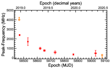
Figure 6: The red-colored points show the measured turnover frequency as a function of epoch. Temporal evolution of the turnover frequency is clearly evident. The orange colored points indicate rough lower or upper limits where the turnover frequency could not be constrained.

We fit the broadband spectra with a spectral shape of the form of a log-parabola as following.

$$\mathop{\log_{10}}S_{\nu}=\beta\times(\mathop{\log_{10}}\nu-\mathop{\log_{10}}\nu_{p})^{2}+C_{0},$$ (1)

where $\nu_{p}$ is the peak frequency corresponding to the turnover, and $\beta$ and $C_{0}$ are constants. The fitted spectra are also shown in Figure 5, overlaid on the data points. The peak frequencies could not be constrained for the broadband spectrum corresponding to MJD 58467 (the first subplot in Figure 5), where it seems to be inverted in the frequency range that the data points span. Subsequently, the next four spectra are reasonably well fit by the above log-parabola model, and the fitted peak-frequency seems to evolve rapidly with time. The next three spectra are also reasonably well fitted with the above model, however, given the spread in our band-3 and band-4 measurements, these spectra might also be consistent with a flattening at low frequencies rather than a turnover in the spectrum. In any case, the fitted peak-frequencies for these three spectra are roughly consistent with each other. For the last broadband spectrum covering the MJD span 59061.78$-$59077.85 (the last subplot in Figure 5), the peak-frequency could not be constrained and the spectrum appears to be steep throughout the frequency range covered by the data points.

From the log-parabola fits of the broadband spectra, it is evident that in about 250 days following the onset of the outburst, the fitted peak-frequency evolves quite rapidly. Thereafter, either the peak-frequency appears to settle down around 500$-$600 MHz or the spectrum becomes flatter at these low frequencies. This trend is evident in Figure 6. The last broadband spectrum in Figure 5, our spectral indices measured using bands 3 and 4 in Figure 3 as well as the flux density measurements shown in Figure 2 suggest that the magnetar exhibits a steep spectrum at later epochs.

5 Discussion

Following the first high-energy outburst, the magnetar XTE J1810$-$197 was detected as a pulsed radio emitter (Camilo et al., 2006), and subsequently observed successfully at radio frequencies as high as 144 GHz, infrared as well as X-rays (e.g., Camilo et al., 2007c). Except for a few observations, the regular monitoring of the magnetar as well as the measurements of its radio spectrum involved frequencies around and higher than 1.4 GHz. Camilo et al. (2007c) monitored the spectrum of the magnetar between May 2006 and November 2006, at frequencies mostly spanning the range 1.4$-$9 GHz. During this time span, the spectrum changed from nearly flat ($\alpha=0$) to steep ($\alpha=-1$). Lazaridis et al. (2008) reported measurements of spectral indices using simultaneous multi-frequency (1.4$-$14.60 GHz) observations between May and July 2006. They showed that overall their measurements were consistent with those from Camilo et al. (2007c). Lazaridis et al. (2008) also reported spectral index measurements obtained using quasi-simultaneous multi-frequency (2.64$-$32 GHz) observations between December 2006 and July 2007. During this time, they reported the spectral indices which appear to gradually increase from around $-0.5$ to $+1.0$. They concluded that overall the spectrum is generally flat, and there is a slight trend of the spectral index becoming positive with time. We note that their observations covered different parts of the above mentioned frequency range at different epochs. Camilo et al. (2016) reported flux densities from their monitoring observations at 1.4 GHz and 2 GHz starting from May 2006 to late 2008 when the radio emission from the magnetar became undetectable. Although their observations were not simultaneous, using the 1.4 and 2 GHz flux density measurements covering similar time-spans, they asserted that the magnetar’s spectrum was steep between early 2007 and late 2008. Note that Lazaridis et al. (2008) reported the spectrum to become flatter or even inverted till about mid-2007, however, their measurements covered a different frequency range.

The above studies provided evidences of significant changes in the magnetar’s radio spectrum during its radio-active phase following the first outburst. However, due to observations covering different frequency ranges, and often at different times, it was not possible to study any underlying gradual evolution of the spectrum with time. Similarly, in this second, ongoing radio-active phase of this magnetar, Eie et al. (2021) have reported their sparse measurements between December 2018 and June 2019 at frequencies of 2.3, 6.9, 8.4 and 22 GHz. Using these measurements and those available from the literature, they have indicated that the magnetar’s radio spectrum has evolved to become steep at Gigahertz frequencies.

Following the second outburst, we have presented our regular monitoring observations of XTE J1810$-$197 in the frequency range 300$-$1450 MHz, along with the spectral indices measured therefrom. Using these measurements, it is evident (see Figure 3) that the magnetar’s spectrum in this frequency range has gradually evolved, from inverted ($\alpha\sim+2$) closer to the onset of the outburst in December 2018 to steep around mid-2019, and quite steep ($\alpha\sim-2$) by early 2021. During this time span, the flux density also shows intriguing trends. After a steep decline following the outburst, the radio flux density shows at least two episodes of re-brightening, one around MJD 58800$-$58850 and another around MJD 59050$-$59150 (Figure 2). There is no hint of enhancement in the X-ray flux during these radio re-brightening episodes (see Figure 17 in Caleb et al., 2021). Absence of any prominent high-energy outbursts suggests that although the radio emission appears following a X-ray outburst, the underlying radio emission processes remain highly dynamic long after the outburst.

As apparent from Figure 3, the temporal evolution of spectral indices measured from different parts of the radio spectrum is slightly different — the higher frequency part of the spectrum seems to become steep earlier than the lower frequency part. A corroborative evidence of this can also be seen in Figure 2 — peak of a short-lived enhancement of flux density during roughly MJD 58500$-$58840 shows up first at band 4 (550$-$750 MHz), and then about 20 days later at band 3. This effect can be explained if the radio spectrum exhibits a spectral turnover with a peak frequency that shifts to lower frequencies with time, an inference that was also discussed by Eie et al. (2021). Using a number of broadband spectra, we have shown that the magnetar exhibits a fast-evolving turnover in its radio spectrum. The peak frequency shifted by nearly a factor of 5 (from $\sim$2.4 GHz to $\sim$500 MHz) in less than 250 days.

5.1 Is a varying spectral turnover an ubiquitous property of magnetars?

A number of radio pulsars exhibit a spectral turnover typically around one or a few GHz (Kijak et al., 2011). Such spectra have been named as gigahertz-peaked spectra (GPS). Out of the five magnetars that are known to exhibit radio emission, the average spectra of three magnetars, PSR J1550$-$5418, PSR J1622$-$4950 and SGR J1745$-$2900 (Kijak et al., 2013; Lewandowski et al., 2015), have also shown the characteristic features of GPS. As we have shown, the magnetar XTE J1810$-$197 also exhibited a turnover at gigahertz frequencies close to the onset of its second outburst. Thus, it joins the group of these GPS pulsars/magnetars. There have been limited broadband radio monitoring observations of magnetars following their outbursts which could probe a spectral turnover evolving as systematically as revealed by our observations. Nevertheless, using archival data at two different epochs, Lewandowski et al. (2015) have claimed to observe a turnover frequency that shifts downwards with time in the spectrum of the Galactic center magnetar SGR J1745$-$2900. Broadband radio monitoring of other magnetars following their future outbursts could reveal if a varying spectral turnover is an ubiquitous property of magnetars.

5.2 Possible physical reasons for the varying spectral turnover

The spectral index evolution presented in Figure 3 exhibits two kinds of variations. First, epoch-to-epoch variations appear to be stochastic in nature, and might be intrinsic to the emission mechanism. The other, long-term observed variations in the spectral index are more gradual. We note that these long-term variations in the spectral index as well as peak-frequency are unlikely to be caused by interstellar scintillation. The diffractive scintillation bandwidth at 650 MHz is estimated to be less than or about 1 kHz, i.e., much smaller than the bandwidths involving our measurements, in the direction of this source (Maan et al., 2019). The transition frequency between the strong and weak scattering in the interstellar medium is estimated to be 50 GHz, i.e., much higher than the frequencies involved in this work. We discuss below two physical explanations of the temporally evolving turnover in the spectrum, and their plausibility.

5.2.1 Thermal absorption; a potential magnetar wind nebulae?

The leading explanation for the GPS feature in pulsar/magnetar spectra is that it originates due to thermal free-free absorption of an otherwise steep spectral emission by dense, ionized gas regions, either in the surrounding environment or along the line of sight. The explanation is motivated by the fact that majority of the GPS sources are located within ionized environments such as pulsar wind nebulae (PWNe), supernovae remnants (SNRs) or HII regions that have high electron densities and emission measures.

Magnetars PSR J1550$-$5418 and PSR J1622$-$4950 are potentially associated with SNRs (Gelfand & Gaensler, 2007; Anderson et al., 2012), making the thermal absorption as a plausible explanation for their GPS features. However, for magnetar SGR J1745$-$2900, there is no known associated SNR or PWN. For this source, Lewandowski et al. (2015) proposed that the absorption is caused by the electron material ejected during the outburst, and the ejecta’s expansion with time could explain the observed change in the peak-frequency.

In case of magnetar XTE J1810$-$197, we have measured the spectral turnover at several epochs and the evolution of the turnover frequency with time is clearly evident. Let us assume a model similar to that proposed by Lewandowski et al. (2015), wherein XTE J1810$-$197 ejected electron material during its second outburst and the turnover is caused by the thermal absorption in this material. Assuming local thermal equilibrium conditions, with quasi-neutral plasma and the electrons that obey the thermal distribution, the spectral turnover frequency, i.e., the frequency corresponding to an optical depth of unity, is given by

$$\frac{\nu_{p}}{GHz}=0.1736\times\frac{T_{e}}{K}^{-3/4}\sqrt{\frac{EM}{pc\,cm^{-6}}<g_{ff}>},$$ (2)

where $T_{e}$ is the electron temperature, $EM$ is the emission measure, and $g_{ff}$ is a correction factor (the Gaunt factor, see Rohlfs & Wilson, 2004, for details). Assuming the correction factor to be unity, and a uniform density profile, i.e., $EM=N_{e}^{2}\delta d$, where $N_{e}$ is the electron density and $\delta d$ is the thickness of the absorber, we have

$$\frac{\nu_{p}}{GHz}=0.1736\times\frac{T_{e}}{K}^{-3/4}\times\frac{N_{e}}{cm^{-3}}\sqrt{\frac{\delta d}{pc}},$$ (3)

Note that a decrease in the turnover frequency, as has been observed, implies either one or a combination of the following: (a) an increase in the electron temperature of the absorbing medium, (b) a decrease in $N_{e}$, (c) a decrease in $\delta d$. It is hard to imagine a way to increase the absorber’s temperature with time, especially as XTE J1810$-$197 is not known to be associated with a SNR or PWN. Moreover, the temporal evolution of the turnover frequency also seem to be linked with that of the outburst. Similar to the model proposed for J1745$-$2900, we can consider the electron material ejected during the XTE J1810$-$197’s outburst and its expansion in a spherical shell to be the cause of the observed shift in the turnover frequency. We do not try to constrain the parameters using this model as more observational information on $T_{e}$, $N_{e}$ and $\delta d$ is needed. Nevertheless, we note that the observed turnover frequencies are possible using the parameter values similar to those considered for J1745$-$2900 by Lewandowski et al. (2015).

We further note that the absorption considered in the above discussed model of the ejecta expanding in a spherical shell is thermal absorption by non-relativistic electrons. However, the electrons in the ejecta from a magnetar’s magnetosphere are expected to be relativistic, which would significantly decrease the absorption efficiency. Hence, the relativistic effects need to be incorporated in optical thickness and absorption efficiency to accurately gauge the likelihood of the the above model explaining the observed varying turnover in the magnetar’s spectrum.

5.2.2 Band-limited emission by varying characteristic energy particles?

The theoretical advances to explain the radio emission characteristics specifically from magnetars have remained limited. There are models that propose radio emission from closed field lines (e.g., Beloborodov, 2009), or, much like radio pulsars, from the open field lines (Szary et al., 2015). However, in these models, there are no specific theoretical predictions for the radio spectrum in general, and an evolving spectral turnover in particular.

There are some key similarities between normal radio pulsars and magnetars, such as the polarization position angle sweeps that can be modelled by the rotating vector model (Radhakrishnan & Cooke, 1969) and highly linearly polarized single pulses with position angles locally following the mean position angle traverse (e.g., Levin et al., 2012), which indicate that the underlying radio emission mechanisms are similar. The leading radio emission mechanism in pulsars is the coherent curvature radiation by particle or soliton bunches (see, e.g., Ruderman & Sutherland, 1975; Melikidze et al., 2000; Mitra et al., 2009). Following Ruderman & Sutherland (1975), the characteristic frequency of single-particle curvature radiation is given by

$$f_{c}=\frac{3c}{2\pi\rho}\gamma^{3},$$ (4)

where $c$ is the speed of light, $\rho$ is the radius of curvature at the emission-site and $\gamma$ is the Lorentz factor of the particle. The exact shape of the observed spectrum is decided by several factors, such as the energy distribution of the particles producing the observed coherent radiation via bunches, the viewing geometry and the range of emission heights, among others.

Here we propose a hypothesis that observed radio emission from the magnetar XTE J1810$-$197 is caused by underlying particles with a narrow energy distribution, and the observed peak in the radio spectrum of the magnetar XTE J1810$-$197 corresponds to the characteristic frequency $f_{c}$. In this highly simplified picture, the observed downward shift in the peak-frequency can be interpreted as a corresponding decrease in the energy of the particle population that gives rise to the observed radiation. As $f_{c}\propto\gamma^{3}$, the observed shift of the peak-frequency by a factor of 5$-$6 needs the population energy to decrease by a factor less than 2.

5.3 Profile width evolution

As apparent from Figure 4, the magnetar’s average profile width shows interesting evolution. Apart of significant short term variations, a trend in the long term is visible. After the outburst, the profile width seems to remain around 20$-$25% of the magnetar’s spin period, albeit with large fluctuations, during the first 350 days or so, until around MJD 58820. Afterwards, the profile width decreases gradually, becoming around 10% of the period in March 2021.

There are expected profile width variations in some magnetar emission models. Beloborodov (2009) proposed a model wherein, following an outburst, the magnetosphere gradually untwists and gives rise to non-thermal radiations preferentially generated on a bundle of extended closed magnetic field lines near the dipole axis. In this model, the radio luminosity as well as the pulse-width is expected to decrease as the bundle shrinks in such a way that most of the radio emission is absorbed within the magnetospheric plasma. While the observed decrease in the pulse-width, particularly at later epochs, seems to be consistent with this picture, we do not see a monotonic decrease in the radio luminosity. Szary et al. (2015) suggest the radio emission from magnetars to originate, much like from normal radio pulsars, from the open field line regions, and explain the emission with the partially screened gap model. However, for the radio emission to be visible, they rely on alteration of the open field line region at the time of outburst to widen the radio beam which causes the radio detection of magnetars in their model. At the time of the outburst, the curvature of open field lines changes significantly, resulting in a much larger opening angle of radio emission. While returning to the quiescent state, the radius of curvature increases back to its original value causing a gradual narrowing of the radio beam, and hence, narrowing of the observed profile width and eventual disappearance of the magnetar. As the predicted behavior is similar in both the models, the observed trend in the profile width does not discriminate between these models.

Overall, the intriguing spectro-temporal evolution uncovered by our low-frequency monitoring of the magnetar XTE J1810$-$197 will hopefully motivate more detailed or even new theoretical modelling of magnetar radio emission. An evolving spectral turnover might be an ubiquitous property of radio magnetars, and our findings strongly advocate systematic radio monitoring of magnetars following their outbursts, preferably using instruments which offer ultra-wide frequency coverages (e.g., Maan et al., 2013; Hobbs et al., 2020).

6 Conclusions

We have presented results from a multi-frequency monitoring campaign of the magnetar XTE J1810$-$197 (PSR J1809$-$1943) with the GMRT covering a frequency range of 300$-$1450 MHz. Based on the flux density measurements at multiple frequencies, we see that the flux density of the magnetar has significantly varied over time at all the frequencies, with multiple episodes of enhanced radio activity. The width of the 550$-$750 MHz average profile shows curious behavior: it remains roughly same for the first 350 days or so, and gradually decreases afterwards. A simple power-law modeling suggests that the magnetar’s radio spectrum has evolved from a flatter or even inverted (magnetar-like) to a steeper (pulsar-like) spectrum with time. A more detailed analysis using broadband spectra reveals an evolving turnover in the spectrum, with the turnover frequency decreasing as a function of time. We propose that the thermal absorption by a piece of the intervening medium, such as the expanding ejecta from the outburst, or a change in the intrinsic emission, such as a hypothetically decreasing energy of the leptons generating the curvature radiation in the magnetosphere, remain plausible physical explanations for the observed spectral behavior.

References

- Anderson et al. (2012) Anderson, G. E., Gaensler, B. M., Slane, P. O., et al. 2012, ApJ, 751, 53, doi: 10.1088/0004-637X/751/1/53
- Beloborodov (2009) Beloborodov, A. M. 2009, ApJ, 703, 1044, doi: 10.1088/0004-637X/703/1/1044
- Caleb et al. (2021) Caleb, M., Rajwade, K., Desvignes, G., et al. 2021, MNRAS, doi: 10.1093/mnras/stab3223
- Camilo et al. (2006) Camilo, F., Ransom, S. M., Halpern, J. P., et al. 2006, Nature, 442, 892, doi: 10.1038/nature04986
- Camilo et al. (2007a) Camilo, F., Reynolds, J., Johnston, S., et al. 2007a, ApJL, 659, L37, doi: 10.1086/516630
- Camilo et al. (2007b) Camilo, F., Cognard, I., Ransom, S. M., et al. 2007b, ApJ, 663, 497, doi: 10.1086/518226
- Camilo et al. (2007c) Camilo, F., Ransom, S. M., Peñalver, J., et al. 2007c, ApJ, 669, 561, doi: 10.1086/521548
- Camilo et al. (2016) Camilo, F., Ransom, S. M., Halpern, J. P., et al. 2016, ApJ, 820, 110, doi: 10.3847/0004-637X/820/2/110
- Dai et al. (2019) Dai, S., Lower, M. E., Bailes, M., et al. 2019, ApJ, 874, L14, doi: 10.3847/2041-8213/ab0e7a
- Duncan & Thompson (1992) Duncan, R. C., & Thompson, C. 1992, ApJ, 392, L9, doi: 10.1086/186413
- Eie et al. (2021) Eie, S., Terasawa, T., Akahori, T., et al. 2021, PASJ, doi: 10.1093/pasj/psab098
- Gelfand & Gaensler (2007) Gelfand, J. D., & Gaensler, B. M. 2007, ApJ, 667, 1111, doi: 10.1086/520526
- Gotthelf et al. (2018) Gotthelf, E. V., Halpern, J. P., Grefenstette, B. W., et al. 2018, The Astronomer’s Telegram, 12297
- Gupta et al. (2017) Gupta, Y., Ajithkumar, B., Kale, H. S., et al. 2017, Current Science, 113, 707, doi: 10.18520/cs/v113/i04/707-714
- Haslam et al. (1982) Haslam, C. G. T., Salter, C. J., Stoffel, H., & Wilson, W. E. 1982, A&AS, 47, 1
- Hobbs et al. (2020) Hobbs, G., Manchester, R. N., Dunning, A., et al. 2020, PASA, 37, e012, doi: 10.1017/pasa.2020.2
- Ibrahim et al. (2004) Ibrahim, A. I., Markwardt, C. B., Swank, J. H., et al. 2004, ApJL, 609, L21, doi: 10.1086/422636
- Joshi et al. (2018) Joshi, B. C., Maan, Y., Surnis, M. P., Bagchi, M., & Manoharan, P. K. 2018, The Astronomer’s Telegram, 12312
- Kijak et al. (2011) Kijak, J., Lewandowski, W., Maron, O., Gupta, Y., & Jessner, A. 2011, A&A, 531, A16, doi: 10.1051/0004-6361/201014274
- Kijak et al. (2013) Kijak, J., Tarczewski, L., Lewandowski, W., & Melikidze, G. 2013, ApJ, 772, 29, doi: 10.1088/0004-637X/772/1/29
- Lazaridis et al. (2008) Lazaridis, K., Jessner, A., Kramer, M., et al. 2008, MNRAS, 390, 839, doi: 10.1111/j.1365-2966.2008.13794.x
- Levin et al. (2012) Levin, L., Bailes, M., Bates, S. D., et al. 2012, MNRAS, 422, 2489, doi: 10.1111/j.1365-2966.2012.20807.x
- Levin et al. (2019) Levin, L., Lyne, A. G., Desvignes, G., et al. 2019, MNRAS, 488, 5251, doi: 10.1093/mnras/stz2074
- Lewandowski et al. (2015) Lewandowski, W., Rożko, K., Kijak, J., & Melikidze, G. I. 2015, ApJ, 808, 18, doi: 10.1088/0004-637X/808/1/18
- Lorimer & Kramer (2004) Lorimer, D. R., & Kramer, M. 2004, Handbook of Pulsar Astronomy, ed. R. Ellis, J. Huchra, S. Kahn, G. Rieke, & P. B. Stetson
- Lyne et al. (2018) Lyne, A., Levin, L., Stappers, B., et al. 2018, The Astronomer’s Telegram, 12284
- Maan et al. (2019) Maan, Y., Joshi, B. C., Surnis, M. P., Bagchi, M., & Manoharan, P. K. 2019, ApJL, 882, L9, doi: 10.3847/2041-8213/ab3a47
- Maan et al. (2021) Maan, Y., van Leeuwen, J., & Vohl, D. 2021, A&A, 650, A80, doi: 10.1051/0004-6361/202040164
- Maan et al. (2013) Maan, Y., Deshpande, A. A., Chandrashekar, V., et al. 2013, ApJS, 204, 12, doi: 10.1088/0067-0049/204/1/12
- Melikidze et al. (2000) Melikidze, G. I., Gil, J. A., & Pataraya, A. D. 2000, ”ApJ”, 544, 1081, doi: 10.1086/317220
- Mitra et al. (2009) Mitra, D., Gil, J., & Melikidze, G. I. 2009, ”APJL”, 696, L141, doi: 10.1088/0004-637X/696/2/L141
- Olausen & Kaspi (2014) Olausen, S. A., & Kaspi, V. M. 2014, ApJS, 212, 6, doi: 10.1088/0067-0049/212/1/6
- Radhakrishnan & Cooke (1969) Radhakrishnan, V., & Cooke, D. J. 1969, Astrophys. Lett., 3, 225
- Ransom (2001) Ransom, S. M. 2001, PhD thesis, Harvard University
- Ransom et al. (2002) Ransom, S. M., Eikenberry, S. S., & Middleditch, J. 2002, AJ, 124, 1788
- Remazeilles et al. (2015) Remazeilles, M., Dickinson, C., Banday, A. J., Bigot-Sazy, M. A., & Ghosh, T. 2015, MNRAS, 451, 4311, doi: 10.1093/mnras/stv1274
- Rohlfs & Wilson (2004) Rohlfs, K., & Wilson, T. L. 2004, Tools of radio astronomy
- Ruderman & Sutherland (1975) Ruderman, M. A., & Sutherland, P. G. 1975, ApJ, 196, 51
- Szary et al. (2015) Szary, A., Melikidze, G. I., & Gil, J. 2015, ApJ, 800, 76, doi: 10.1088/0004-637X/800/1/76
- Torne et al. (2020) Torne, P., Macías-Pérez, J., Ladjelate, B., et al. 2020, A&A, 640, L2, doi: 10.1051/0004-6361/202038504
- Torne et al. (2022) Torne, P., Bell, G., Bintley, D., et al. 2022, arXiv e-prints, arXiv:2201.07820. https://arxiv.org/abs/2201.07820
- Trushkin et al. (2019) Trushkin, S. A., Bursov, N. N., Tsybulev, P. G., Nizhelskij, N. A., & Erkenov, A. 2019, The Astronomer’s Telegram, 12372
- van Straten & Bailes (2011) van Straten, W., & Bailes, M. 2011, PASA, 28, 1, doi: 10.1071/AS10021