Experimental Demonstration that
No Tripartite-Nonlocal Causal Theory Explains Nature’s Correlations

Abstract

Quantum theory predicts the existence of genuinely tripartite-entangled states, which cannot be obtained from local operations over any bipartite entangled states and unlimited shared randomness. Some of us recently proved that this feature is a fundamental signature of quantum theory. The state $\left|{\rm GHZ}_{3}\right\rangle=(\left|000\right\rangle+\left|111\right\rangle)/\sqrt{2}$ gives rise to tripartite quantum correlations which cannot be explained by any causal theory limited to bipartite nonclassical common causes of any kind (generalising entanglement) assisted with unlimited shared randomness. Hence, any conceivable physical theory which would reproduce quantum predictions will necessarily include genuinely tripartite resources.

In this work, we verify that such tripartite correlations are experimentally achievable. We derive a new device-independent witness capable of falsifying causal theories wherein nonclassical resources are merely bipartite. Using a high-performance photonic $\left|{\rm GHZ}_{3}\right\rangle$ states with fidelities of $0.9741\pm 0.002$, we provide a clear experimental violation of that witness by more than 26.3 standard deviation, under the locality and fair sampling assumption. We generalise our work to the $\left|{\rm GHZ}_{4}\right\rangle$ state, obtaining correlations which cannot be explained by any causal theory limited to tripartite nonclassical common causes assisted with unlimited shared randomness.

mltΘ

Introduction.— Since its inception, quantum theory has been remarkably successful in explaining and predicting various phenomena, such as the black-body radiation, the energy levels of the hydrogen atom, and more recently the violation of Bell inequalities [1]. Every prediction of quantum theory which has been subjected to experimental testing has been validated, sometimes to record-breaking precision. General consensus among scientists is that the operational predictions of quantum theory are no longer in question, at least in regimes accessible with current technologies.

However, empirical success need not imply ontological truth. Accordingly, physicists remain motivated to explore alternatives to quantum theory, to either subsume or replace it. There are several motivations for such considerations. Firstly, the mathematical formalism of quantum theory is the first representation of Nature to reject the intuitive local realistic approach of all previous physical theories. Secondly, efforts to construct alternatives to quantum theory have historically proven quite fruitful in enlightening our understanding of quantum theory by contrast [2, 3]. Finally, there are serious obstacles to reconciling quantum theory with general relativity [4]. Some paradoxes admit multiple potential resolutions, but there are ongoing efforts to either quantize gravity [5, 6] or to generalize quantum theory [7, 8].

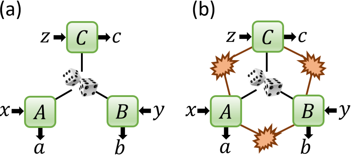
Figure 1: Bell’s theorem rules out any explanation of tripartite quantum correlations in terms of unbounded shared randomness (also called local-hidden-variable models), represented in (a) as dice.                                                                    In this letter we rule out the stronger model depicted in (b). Measuring a $\left|\rm{\rm GHZ}_{3}\right\rangle$ state, we obtain correlations that cannot be explained by any theory based on unbounded shared randomness (represented as dice) and any exotic generalisation of bipartite-entangled states (represented as starbursts). We further generalise our setup to the $\left|{\rm GHZ}_{4}\right\rangle$ state, ruling out any theory based on unbounded shared randomness and generalisations of tripartite-entangled states.

At the heart of what makes quantum theory nonclassical lies entanglement, a fundamental concept in quantum theory which underlies many non-classical behaviours (i.e. many quantum phenomena), such as nonlocality [9]. The existence of this property of quantum correlations was first demonstrated by Bell with his eponymous theorem [10, 11]. It shows that two parties measuring a maximally entangled source can obtain nonlocal correlations, which resist any explanation in terms of local-hidden-variable models. This was verified in several celebrated Bell experimental tests, namely in loophole-free CHSH violations [12, 13, 14, 15, 16, 17, 18, 19].

As a consequence, no predictive theory of Nature’s correlations can avoid introducing bipartite nonlocal resources, namely states shared by two parties that admit no description in terms of classical randomness, i.e that are not reproducible by local-hidden-variable models. In the formalism of quantum theory this role is fulfilled by bipartite entanglement, but any potential theory that would replace quantum theory will necessary include a resource akin to quantum bipartite entanglement, such as the Popescu-Rohrlich box [3].

However, the formalism of quantum theory admits nonclassical resources beyond bipartite entanglement. It postulates the existence of states which are so-called genuinely network tripartite-entangled, i.e. states which cannot be obtained by three parties through Local Operations (LO) on bipartite entangled sources and Shared Randomness (SR) [20]. The $\left|{\rm GHZ}_{3}\right\rangle=\frac{1}{\sqrt{2}}(\left|000\right\rangle+\left|111\right\rangle)$ state is such an example. In other terms, quantum theory’s mathematical formalism includes 3-way entanglement as an additional resource, strictly stronger than bipartite entanglement. This greater resource underlies operational predictions that are qualitatively stronger than bipartite resources, such as a stronger version of Bell’s theorem [21].

Note that the intrinsicness of genuinely tripartite-entangled resources in quantum theory does not a priori necessitate the existence of such resources in future alternatives to quantum theory. For instance, although $\left|{\rm GHZ}_{3}\right\rangle$ is required to achieve maximal violation of the Mermin inequality within quantum theory, one can also reproduce the same operational correlations by means exclusively bipartite resources in alternative physical theories such as Boxworld [22, 23] (see Fig. 1b). Might a future theory explain all of Nature’s tripartite correlations without invoking any intrinsically tripartite nonclassical states? Formally, would it be possible to simulate all tripartite quantum correlations from theories restricted to the sort of bipartite exotic nonclassical states which generalising bipartite entanglement, supplemented with unlimited shared randomness?

In Refs. [24, 25], some of us developed a test to disprove any such explanation. This test can be seen as a generalisation of Bell’s theorem: not only do we disprove any explanation in terms of unbounded shared randomness (also called local-hidden-variable models), but we also disprove any explanation relying on a yet-to-be-discovered causal theory that would involve exotic bipartite nonclassical resources and unbounded shared randomness, such as presented in Fig. 1b. Our test is predicated on the nonfanout inflation technique [26], which minimally assumes that a future theory should satisfy causality and allow for device replication [27, 28, 29, 30].

In this letter, our first main result is the computer-aided derivation of an improved test which is maximally robust against general noise models. The potential experimental demands for violating this new inequality are significantly reduced compared to the inequality derived in Ref. [24]. Then, in our second main result, we report an experimental demonstration of said inequality’s violation using a photonic setup to experimentally exhibit correlations that cannot be explained by any theory based on shared randomness and bipartite nonlocal resources, however exotic. Furthermore, we expand both our witness derivation and experimental demonstration to the $\left|{\rm GHZ}_{4}\right\rangle=\frac{1}{\sqrt{2}}(\left|0000\right\rangle+\left|1111\right\rangle)$ state, proving that it realizes correlations which cannot be explained neither by any theory relying on shared randomness and, this time, tripartite exotic nonlocal resources. Hence, we show experimentally that no tripartite-nonlocal causal theory can explain Nature’s correlations.

The ideal protocol.— Here, we first propose a concrete experimental procedure which is a variant of the protocols of Refs. [24, 25]. Then, we show that it is a valid test to disprove any explanation based on bipartite exotic nonclassical states and unlimited shared randomness.

A $\left|{\rm GHZ}_{3}\right\rangle$ state is distributed to Alice, Bob, and Charlie. The players perform independent measurements depending on their respective uniformly distributed random inputs $x,y,z\in\{0,1\}$. They produce respective outputs $a,b,c\in\{\pm 1\}$. Alice’s and Charlie’s respective measurements are $(\sigma_{z},\sigma_{x})$, and Bob’s respective measurements are $(\frac{\sigma_{x}+\sigma_{z}}{\sqrt{2}},\frac{\sigma_{x}-\sigma_{z}}{\sqrt{2}})$.

In Appendix B we extend Algorithm 1 from Ref. [25, Sec. IV] in order to obtain inequalities maximally robust against general noise models. We obtain the following novel inequality satisfied by any strategy based on any bipartite-nonlocal exotic resources and unrestricted shared randomness:

$$\begin{aligned} W_{3}\coloneqq&\langle A_{0}B_{0}\rangle+\langle B_{0}C_{0}\rangle-\langle A_{0}B_{1}\rangle-\langle B_{1}C_{0}\rangle\\ &+4\langle A_{0}C_{0}\rangle+2\langle A_{1}B_{0}C_{1}\rangle+2\langle A_{1}B_{1}C_{1}\rangle~{}~{}\leq~{}8\end{aligned}$$ (1)

The considered tripartite quantum strategy gives a violation of ${W_{3}\to 4+4\sqrt{2}\approx 9.657}$. Under white noise $W_{3}$ evaluates to zero, implying a visibility against white noise of $v\gtrsim 0.828$.

We generalize this to four players, with the shared quantum state $\left|{\rm GHZ}_{4}\right\rangle$, adding a fourth player named Dave. The generalized quantum strategy keeps Alice, Bob and Charlie as before, while Dave behaves as Charlie, measuring $(\sigma_{z},\sigma_{x})$ with inputs $w\in\{0,1\}$ and outputs $d\in\{\pm 1\}$. Following the same technique, we obtain the following novel inequality satisfied by any strategy based on any tripartite-nonlocal exotic resources and unrestricted shared randomness:

$$\begin{aligned} W_{4}\coloneqq\langle A_{0}B_{0}\rangle&-\langle A_{0}B_{1}\rangle+2\langle A_{0}D_{0}\rangle+2\langle C_{0}D_{0}\rangle\\ &\hskip 4.30554pt+\langle A_{1}B_{0}C_{1}D_{1}\rangle+\langle A_{1}B_{1}C_{1}D_{1}\rangle~{}~{}\leq~{}6~{}~{}\end{aligned}$$ (2)

The quadpartite quantum strategy gives a violation of ${W_{4}\to 4+2\sqrt{2}\approx 6.828}$, with white noise visibility $v\gtrsim 0.879$.

Figure 2: Scheme of the $\left|{\rm GHZ}_{4}\right\rangle$ experiment. The sandwich-like BBO resource consists of BBO-HWP-BBO configuration. In each source, two possible ways of down conversion may occur in former and latter BBO. They are made indistinguishable by the temporal and spatial compensation crystal in both arms. A 1nm (3nm) width spectral filter is inserted in the extraordinary (ordinary) photon before measurement to enhance the fidelity of the entangled state. The SPDC sources combined with the HOM interference corresponds to the multipartite entangled resources with shared randomness while the local measurement setting embedded in blacked boxes plays the role of the parties. For the $\left|{\rm GHZ}_{3}\right\rangle$ experiment, Dave projects over the diagonal basis $\left|+\right\rangle$.

The experiment.— We experimentally implement this protocol in a photonic platform, based on the spontaneous parametric down-conversion process (SPDC). The experimental setup is illustrated in Fig. 2. We first generate polarization twin photons by adopting the sandwich-geometry beam-like type-II SPDC [31, 32]. A frequency doubled pulsed ultraviolet laser with 390nm central wavelength is focused on sandwich-like combination of $\beta$-barium-borate (BBO) crystal to generate the maximally entangled state in polarization. A half-wave-plate (HWP) transforms the down-converted entangled photon into $\left|\psi\right\rangle=\left(\left|00\right\rangle+\left|11\right\rangle\right)/\sqrt{2}$. Here we encode logic qubit $\left|0\right\rangle$ ($\left|1\right\rangle$) in horizontal (vertical) polarization respectively. For preparing a 4-photon (or 3-photon) GHZ state, two pairs of entangled states are generated by sequentially pumping two SPDC sources, and the extraordinary photons in each source are spatially overlapped in polarization beam splitter (PBS) to complete the Hong-Ou-Mandel (HOM) interference. A trombone-arm delay line is introduced to make interfering photons indistinguishable in arrival time. The PBS acts as a parity check operation on interfering photons. The $\left|{\rm GHZ}_{4}\right\rangle$ state is obtained by collectively post-selecting on one photon for all parties. Each party is capable of performing arbitrary local measurement on received qubit by polarization analyzing system consisting of a quarter-wave plate (QWP), a HWP, and a PBS. At last, the $\left|{\rm GHZ}_{3}\right\rangle$ state is obtained by post selecting on one of the photons being measured into diagonal basis $\left|+\right\rangle$.

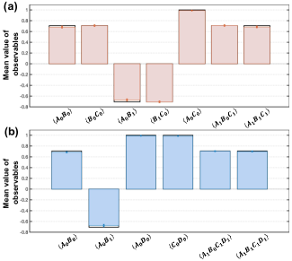
Figure 3: Experimental results for the 3-photon (a) and 4-photon (b) GHZ states, for all terms involved in the inequalities (1) and (2) . Theoretically predictions are plotted with transparent pillars and experimental values in nontransparent ones. The errorbars are computed through a Monte Carlo simulation to evaluate the Poisson noise of the photonic statistics.

The results.— In designing an experiment to achieved the requisite fidelity, we note that the dominant obstacles to inequality violation is white noise related to higher-order emission. To suppress the higher-order emission noise we therefore maintain the experimental operation in low pumping power yielding an approximate four-fold counting rate of 1 click/s. The quantum measurement strategy was optimized to maximally violate the inequality, following the aforementioned protocol.

We evaluate the experimental violations of the two inequalities given by Eq. (1) and Eq. (2) for our experimental sources of 3-photon and 4-photon GHZ states, terms by terms. The mean values of each term is given in Fig. 3. Thanks to the high performance of our sources, our experimental mean values are in good agreement with the theoretical predictions for ideal GHZ states. We obtain the violations

$$W_{3}=9.5150\pm 0.0576,$$ (3)

with more than 26.3 standard deviation, and

$$W_{4}=6.7154\pm 0.0256,$$ (4)

with more than 27.9 standard deviation. These significant violations provide strong support for the idea that correlations achieved via 3-photon (and 4-photon) GHZ state cannot be explained by bipartite-nonlocal (resp. tripartite-nonlocal) causal theories.

Discussion.— First, note that our protocol can be generalised to any number of parties. For instance, one could in principle generalise our experiment to the $\left|{\rm GHZ}_{5}\right\rangle$ state. Of course, to do so we would first need to isolate a suitable inequality to test against. We found our algorithmic approach to inequality derivation to be intractable for such large $N$, even with symmetry reduction. We have identified a new family of inequalities which is slightly too demanding in terms of noise with respect to our experimental setup (see discussion in Appendix D). We suspect that it is possible to obtain new inequalities, maybe including extra measurements for the parties, which would reduce the critical fidelity requirements to what is achievable with current technologies for the $\left|{\rm GHZ}_{5}\right\rangle$ and $\left|{\rm GHZ}_{6}\right\rangle$ states.

Our experimental demonstration admits two common loopholes considered in Bell nonlocality experiments: the locality loophole and the postselection loophole. We now briefly discuss the theoretical reasons why these loopholes might undermine our conclusions, why we consider these loopholes implausible, and how these loopholes might be closed in future experiments.

In an alternate universe in which Nature would not admit genuinely multipartite nonlocal sources, our experiment can still be simulated if any party’s measurement outcomes were allowed to causally depend on the other parties’ choices of measurement settings. This is our locality loophole. It is standard to assume locality in a Bell experiment. Ghostly influence from one measurement apparatus to another is theoretically conceivable, but practically implausible. Nevertheless, the locality loophole can in-principle be closed in a future experiment, by enforcing a space-like separation of the parties, which is accessible to current technologies [33].

Another loophole which could explain away our experimental data without requiring genuinely multipartite nonlocal sources is the postselection loophole. After all, in our final analysis, we exclusively considered the subset of trials in which all every party received exactly a photon. Postselection could artificially simulate our experimental data if the detection versus nondetection determination for a given party is allowed to causally depend on that party’s choice of measurement setting. The assumption that each party’s ‘detection’ random variable is causally independent of their setting variable is known as fair sampling; the fair sampling assumption is quite commonly employed in photonic experimental investigations of nonlocality. However, fair sampling by itself does not entirely close the postselection loophole. Indeed, one can simulate all statistics arising from measurements on $\left|{\rm GHZ}_{3}\right\rangle$ using strictly bipartite sources if one allows for postselection, even under the constraint that the postselection variable is causally independent of the measurement settings. As such, the conclusion that our experimental results demonstrate the presence of genuinely multipartite nonlocal sources hinges on one additional assumption, beyond just locality and fair sampling. This further assumption is that it is possible — in the exotic foil theories under consideration — to move any postselection process from the measurements to the sources without modifying the measurement statistics. This theory-agnostic assumption codifies our belief that — even though we utilized postselection at the measurements — Nature would allow for a reproduction of our experiment with postselection at the sources, i.e., with heralded event-ready sources.

This postselection loophole might be closed in a future experiment by preparing the $\left|{\rm GHZ}_{3}\right\rangle$ (resp. $\left|{\rm GHZ}_{4}\right\rangle$) state in a heralded event-ready preparation using three (resp. four) cascaded SPDC sources. This would generalise the work of [34], where two cascaded SPDC sources are used to obtain a heralded EPR pair. Current hardware, however, is insufficient for preparing heralded multipartite entanglement sources capable of achieving required noise tolerance and creation rates.

Conclusion.— In this letter, we experimentally demonstrated that any causal theory that aims to explain all possible correlations of Nature must include genuinely tripartite-nonlocal and four-partite-nonlocal states. In quantum theory, this role is taken by what we call genuinely LOSR (network) tripartite and fourpartite entangled states already introduced in Ref. [20]. We have also shown how to improve the algorithm of [25] to obtain inequalities maximally robust against general noise models and white noise models, reducing the demand in computing power by exploiting the symmetries of the problem. We expect this method to be fundamental for future (loophole free) demonstrations of Nature multipartie nonlocal genuiness.

Note that this LOSR-based definition is more restrictive than the traditional LOCC-based definition of genuine tripartite entanglement due to Seevinck and Uffink [35]. Let us first emphasize that this traditional definition is not adapted to the no-signalling context. Indeed, a four-qubit state composed of a singlet shared between Alice and Bob as well as a singlet shared between Bob and Charlie satisfies Seevinck’s criterion for genuinely tripartite entanglement, despite being created from bipartite entanglement. In the same way, the definition of LOSR multipartite genuine nonlocality that we adopt in our letter is more restrictive than the traditional definition of genuine tripartite nonlocality due to Svetlichny [36]. The traditional definition is susceptible to precisely the same sort of hacking: the tripartite correlations obtained from two parallel CHSH violations between Alice and Bob as well as between Bob and Charlie are genuinely tripartite nonlocal according to Svetlichny’s criterion.

These two historical definitions of genuine multipartiteness for nonlocality and entanglement are ill-suited for our study because they were motivated by quantifying resourcefulness relative to Local Operations and Classical Communication (LOCC). However, when analysing Bell-inequality violations, we assume that the involved parties are spacelike separated, and this enforces the No-Signalling condition. When classical communication is forbidden, the only form of nonclassical-resources processing that remains is via Local Operations and Shared Randomness (LOSR). This new approach is closely related to the concept of network nonlocality which has been extensively studied in the past decade [37, 38, 39, 40].

The use of the traditional notions of multipartite genuine entanglement and nonlocality for analysing the states and correlations obtained in various multipartite experiments is widespread. Let us conclude by saying that the use of these notions should be questioned in light of the context of the experiment in which they are used, keeping in mind that they are not adapted to the No-signalling context  [41, 42].

Note added.— While finishing this manuscript, we became aware of related work by Ya-Li Mao et al. [43].

Acknowledgements.— We thank Antonio Acín and Enky Oudot for valuable discussions. This research was supported by the Swiss National Science Foundation (SNF) and Perimeter Institute for Theoretical Physics. Research at Perimeter Institute is supported in part by the Government of Canada through the Department of Innovation, Science and Economic Development Canada and by the Province of Ontario through the Ministry of Colleges and Universities. M.-O.R. is supported by the Swiss National Fund Early Mobility Grants P2GEP2_19144 and the grant PCI2021-122022-2B financed by MCIN/AEI/10.13039/501100011033 and by the European Union NextGenerationEU/PRTR, and acknowledges the Government of Spain (FIS2020-TRANQI and Severo Ochoa CEX2019-000910-S [MCIN/ AEI/10.13039/501100011033]), Fundació Cellex, Fundació Mir-Puig, Generalitat de Catalunya (CERCA, AGAUR SGR 1381) and the ERC AdG CERQUTE. This research was supported by the National Key Research and Development Program of China (No. 2017YFA0304100), the National Natural Science Foundation of China (Nos. 11774335, 11821404, 11734015, 62075208).

Contributions.— H.C., M-O.R. and C.Z contributed equally to this work.

oneΔ

Appendix A Experimental details

EPR source.— A sandwich-like structure crystal is used to generate polarization-entangled photon pairs, which consists of two adjacent, 1-mm-thick $\beta$-barium borate (BBO) crystals and a true-zero-order half-wave plate (THWP) inserted in the middle. The two BBO crystals (BBO1 and BBO2) are identically cut with beamlike type-II phase-matching and their optical axes are parallel in the horizontal plane. Thus BBO1 and BBO2 both produce photon pairs in the polarization state $|H\rangle_{e}|V\rangle_{o}$, the subscript o (e) denotes the ordinary (extraordinary) photon with respect to the crystal. The THWP rotates the polarization of the photon pairs produced by BBO1 to the orthogonal state $|V\rangle_{e}|H\rangle_{o}$. When the two possible ways of generating photon pairs (in BBO1 and BBO2 respectively) are made indistinguishable by spatial and temporal compensations, the photon pairs are prepared in entangled state $\frac{1}{\sqrt{2}}(|H\rangle_{e}|V\rangle_{o}-|V\rangle_{e}|H\rangle_{o})$.

GHZ states preparation.— As shown in Fig.1 of the main text, we use two EPR sources to produce the three- and four-photon GHZ states. The laser pulse from a mode-locked Ti:sapphire laser (with a central wavelength of 780 nm, a pulse duration of 140 fs, a repetition rate of 80 MHz) is first frequency doubled to 390 nm and then pumps the two sources sequentially. We initialize the two EPR sources to both produce polarization state $\frac{1}{\sqrt{2}}(|H\rangle_{e}|H\rangle_{o}+|V\rangle_{e}|V\rangle_{o})$. Then the two e-polarized photons are directed to overlap on a PBS. It is possible to check that when there is one and only one photon in each output, only two terms $|HHHH\rangle$ and $|VVVV\rangle$ are post-selected. The two terms are further made indistinguishable by interference on the PBS, thus the initial product state is projected into the four-photon GHZ state $\frac{1}{\sqrt{2}}(|HHHH\rangle+|VVVV\rangle)$. The three-photon GHZ state can be prepared by projecting the last photon on $|+\rangle$. In our experiment, the postselection is realized by post-processing the detected data after the experiment is finished. Note that by using auxiliary photons and quantum teleportation we can detect a single photon without destroying it and keeping its quantum information intact, thus the postselection can be realized in principle in the state preparation part and lead to a heralded GHZ state.

Detection.— In the measurement part, each photon is first passed through an interference filter (IF), we use 1- and 3-nm bandwidths filters for e- and o-polarized photons respectively. Then each photon is detected by a polarization analysis system which consists of one QWP, one HWP, one PBS and two fiber-coupled single-photon detectors. In the experiment, we use a low pump power of 60 mW to limit the higher-order emission noise in SPDC. The two-photon counting rate is about 12000 Hz and four-photon counting is about 1 Hz. To measure the LOSR inequalities, we perform several local measurement settings, and record all combinations of the four-fold coincidence events by using a coincidence unit (UQDevice), with a coincidence window of 4 ns. The raw data is shown in Table I.

Table 1: Raw data for local measurement settings. X and Z are Pauli operators. Here we use “+(-)” to denote the +1(-1) port detector firing for each photon. The data collection time for ZZZZ and ZZZX is 20000s, the other settings is 4000s.

Setting	++++	+++-	++-+	++- -	+-++	+-+-	+- -+	+- - -	-+++	-++-	-+-+	-+- -	- -++	- -+-	- - -+	- - - -
$X\frac{(Z+X)}{\sqrt{2}}XX$	439	72	84	414	67	516	412	69	94	374	402	74	433	83	43	389
$X\frac{(Z-X)}{\sqrt{2}}XX$	62	372	376	73	400	77	71	413	356	59	79	371	67	454	354	65
$Z\frac{(Z+X)}{\sqrt{2}}XX$	390	371	395	336	78	78	81	66	53	69	71	56	364	372	351	371
$Z\frac{(Z-X)}{\sqrt{2}}XX$	369	366	411	384	87	70	75	97	67	59	56	53	351	367	337	359
$XXXX$	450	5	11	451	9	513	531	7	4	430	428	9	499	5	9	461
$ZZZZ$	8552	16	13	0	9	11	14	18	15	19	11	13	0	19	20	8311
$ZZZX$	5229	4651	7	6	19	22	20	24	19	21	28	20	11	10	4426	4861
$X\frac{(Z+X)}{\sqrt{2}}ZX$	403	406	72	83	73	71	412	427	443	429	74	66	68	81	438	422
$X\frac{(Z-X)}{\sqrt{2}}ZX$	422	443	85	66	66	62	424	400	415	420	76	82	62	71	394	422

Characterization of the prepared states.— From the measurement result of XXXX, we know that the HOM interference visibility in our experiment is at least $0.9691\pm 0.0041$. From the measurement results of XXXX and ZZZZ, we can give a lower bound on the state fidelity according to the two setting entanglement witness

$$\mathcal{W}_{\mathrm{GHZ}_{\mathrm{N}}}:=3\mathbb{I}-2\left[\frac{S_{1}^{\left(\mathrm{GHZ}_{N}\right)}+\mathbb{I}}{2}+\prod_{k=2}^{N}\frac{S_{k}^{\left(\mathrm{GHZ}_{N}\right)}+\mathbb{I}}{2}\right]$$ (5)

where

$$\begin{array}[]{l}S_{1}^{\left(\mathrm{GHZ}_{\mathrm{N}}\right)}:=\prod_{k=1}^{N}X^{(k)}\\ S_{k}^{\left(\mathrm{GHZ}_{\mathrm{N}}\right)}:=Z^{(k-1)}Z^{(k)}\quad\text{ for }k=2,3,\ldots,N.\end{array}$$ (6)

are stabilizers for GHZ state. The measured result is $\langle\mathcal{W}_{\mathrm{GHZ}_{\mathrm{4}}}\rangle=-0.9482\pm 0.0048$. Then we can deduce the state fidelity $F=\langle\mathrm{GHZ}_{4}|\rho_{\mathrm{exp}}|\mathrm{GHZ}_{4}\rangle>(1-\langle\mathcal{W}_{\mathrm{GHZ}_{\mathrm{N}}}\rangle)/2=0.9741\pm 0.0024$. We also perform a quantum state tomography to characterize the prepared state, the reconstructed density matrix is shown in Fig.4. The state fidelity is calculated to be $0.9762\pm 0.0032$, which agrees with the above result very well.

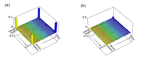
Figure 4: (a) Real and (b) Imaginary part of the reconstructed density matrix of the prepared four-photon GHZ state.

Appendix B General Robustness and Specific Noise Models

This discussion presumes prior understanding of Algorithm 1 from Ref. [25, Sec. IV]. There, some of us introduced a technique to find constraints over distributions obtainable from $(N{-}1)$-way nonlocal resources and unrestricted shared randomness. Given a nonfanout inflation of the $(N{-}1)$-way nonlocal resources model (see Ref. [25, Fig. 1]), we exhibit a Linear Programming (LP) test providing necessary satisfiability constraints. More precisely, if a given correlation $P_{A_{1}...A_{N}|X_{1}...X_{N}}$ can be obtained from $(N{-}1)$-way nonlocal resources and unrestricted shared randomness, one could in principle duplicate the building blocks used to obtain it and replace them in the nonfanout inflated scenario. In this new scenario, one would observe a new correlation satisfying some linear compatibility constraint with the inflated scenario itself, and with $P_{A_{1}...A_{N}|X_{1}...X_{N}}$. If these linear constraints cannot be satisfied, then it proves that $P_{A_{1}...A_{N}|X_{1}...X_{N}}$ is not compatible with $(N{-}1)$-way nonlocal resources and unrestricted shared randomness. These linear constraint form the following LP:

$\textbf{LP}_{sat}$:

We say that $\vec{P}\propto\textbf{LP}_{sat}$ if and only if

• there exists some non-negative vector $\vec{x}$ such that

• for matrix $M_{1}$ we satisfy $M_{1}\cdot\vec{x}=\vec{P}$ and

• for matrix $M_{2}$ we satisfy $M_{2}\cdot\vec{x}=\vec{0}$.

When referring to normalized mutlipartite correlation vectors, we use the notation ${\vec{P}\in\textbf{LP}_{sat}}$ instead of ${\vec{P}\propto\textbf{LP}_{sat}}$.

In this notation $M_{1}$ is a marginalization matrix capturating the fact that the observed probabilities must arise as the marginals of some nonfanout inflation, and $M_{2}$ is a matrix capturing other equality constraints such as the fact that all inflations admit nonsignalling correlations, and that various marginals of different nonfanout inflations must coincide; see Ref. [25, Algorithm 1]. Of course, the linear program implied by nonfanout inflation is itself a relaxation of true causal compatibility. That is, $\vec{P}\not\in\textsf{LOSR\_Genuinely\_Multipartite}\implies\vec{P}\in\textbf{LP}_{sat}$, but not not vice versa.

In this work, however, we do not merely want to test whether or not a given correlation vector $\vec{P}$ satisfies the linear programming constraints. Instead, our goal is to use linear programming to extract an inequality showing that $\vec{P}$ cannot satisfy the linear programming constraints, and moreover our inequality should be maximally robust against general noise.

Firstly, let us recast the satisfiability problem as an optimization problem. The visibility $v^{\star}(\vec{P})$ against general noise models is the largest real number $v$ such that ${v{\times}\vec{P}{+}(1{-}v){\times}\vec{P^{\prime}}}\not\in\textsf{LOSR\_Genuinely\_Multipartite}$ (for any normalized correlation $\vec{P^{\prime}}$). Relative to the LP relaxation, however, we define $v^{\star}_{\text{LP}}(\vec{P})$ as the largest real number $v$ such that ${v{\times}\vec{P}{+}(1{-}v){\times}\vec{P^{\prime}}}\in\textbf{LP}_{sat}$. Linearity of the definition implies that one can restrict $\vec{P^{\prime}}$ to be normalized and nonsignalling whenever $\vec{P}$ is normalized and nonsignalling without loss of generality, since all correlations in the set $\textbf{LP}_{sat}$ are normalized and nonsignalling. Plainly $v^{\star}_{\text{LP}}(\vec{P})\geq v^{\star}(\vec{P})$. However, even this inflation-related optimization problem is apparently nonlinear, as it involves a product of the target variable $v$ with the unspecified probabilities in $\vec{P^{\prime}}$. We get around this by recognizing that the following formulations of $v^{\star}_{\text{LP}}(\vec{P})$ are equivalent.

$$v^{\star}_{\text{LP}}(\vec{P}) \coloneqq\max_{v,\vec{P^{\prime}}}\left(v\;\middle|\;\vec{P^{\prime}}\geq\vec{0},\,{v{\times}\vec{P}{+}(1{-}v){\times}\vec{P^{\prime}}}\in\textbf{LP}_{sat}\right), \text{ with }\left\lVert*\right\rVert{\vec{P^{\prime}}}{=}1\text{ implicit,}$$ (7a)

$$=\max_{v,\vec{s}}\left(v\;\middle|\;\vec{s}\geq\vec{0},\,{v{\times}\vec{P}{+}\vec{s}}\in\textbf{LP}_{sat}\right), \text{with }\left\lVert*\right\rVert{\vec{s}}{=}1{-}v\text{ implicit,}$$ (7b)

$$=\max_{\vec{s}}\left(\left\lVert*\right\rVert{\vec{P}{+}\vec{s}}^{-1}\;\middle|\;\vec{s}\geq\vec{0},\,{\vec{P}{+}\vec{s}}\propto\textbf{LP}_{sat}\right), \text{with unrestricted }\left\lVert*\right\rVert{\vec{s}}{\in}[0,\inf)\,,$$ (7c)

$$=\left(\min_{\vec{s}}\left(\left\lVert*\right\rVert{\vec{P}{+}\vec{s}}\;\middle|\;\vec{s}\geq\vec{0},\,{\vec{P}{+}\vec{s}}\propto\textbf{LP}_{sat}\right)\right)^{-1}$$ (7d)

We therefore implement the final formulation, making use of a constant-valued vector $\vec{c}$ such that $\vec{c}\cdot\vec{x}=1$ if $\vec{x}$ is normalized.

$\textbf{LP}_{opt,primal}$:

The visibility $v^{\star}_{\text{LP}}(\vec{P})$ against general noise models is equal to $\frac{1}{\tau_{\text{primal}}(\vec{P})}$, where $\tau_{\text{primal}}(\vec{P})\coloneqq{\displaystyle\min_{\vec{x}}\;\vec{c}\cdot\vec{x}}$ such that

• $\vec{x}\geq\vec{0}$ and

• $M_{1}\cdot\vec{x}\geq\vec{P}$ and

• $M_{2}\cdot\vec{x}=\vec{0}$.

We can now dualize that linear program. Let $\vec{y_{1}}$ be the dual vector associated with the rows of $M_{1}$, and let $\vec{y_{2}}$ be the dual vector associated with the rows of $M_{2}$. Then,

$\textbf{LP}_{opt,dual}$:

The visibility $v^{\star}_{\text{LP}}(\vec{P})$ against general noise models is equal to $\frac{1}{\tau_{\text{dual}}(\vec{P})}$, where $\tau_{\text{dual}}(\vec{P})\coloneqq{\displaystyle\max_{\vec{y_{1}},\vec{y_{2}}}\;\vec{y_{1}}\cdot\vec{P}}$ such that

• $\vec{y_{1}}\geq\vec{0}$ and $\vec{y_{2}}\geq\vec{0}$ and

• $M_{1}^{T}\cdot\vec{y_{1}}+M_{2}^{T}\cdot\vec{y_{2}}\leq\vec{c}$.

LP duality guarantees that $\tau_{\text{primal}}(\vec{P})=\tau_{\text{dual}}(\vec{P})$ [45]. The inequality resulting from the dual formulation is that $\vec{y_{1}}\cdot\vec{P}\leq 1$ for all $\vec{P}\in\textbf{LP}_{sat}$, and moreover, for $\vec{P}\not\in\textbf{LP}_{sat}$ we have $\vec{y_{1}}\cdot\vec{P}=\frac{1}{v^{\star}_{\text{LP}}(\vec{P})}>1$. Note that our inequalities must have nonnegative coefficients associated with event probabilities. The negative coefficients for the inequalities presented in the main text (as well as the bounds being different from unity) are consequences of the authors’ choice to represent the inequalities in terms of expectation values instead of probabilities, motivated by compactness of presentation.

The visibility of a correlations against general noise models is generally more demanding (i.e., higher visibility) than against particular noise models. Visibility against a particular noise model $P^{\prime}$ is given by

$$\begin{split}v^{\star}(\vec{P},\vec{P^{\prime}})&\coloneqq\max_{v}\left(v\;\middle|\;{v{\times}\vec{P}{+}(1{-}v){\times}\vec{P^{\prime}}}\not\in\textsf{LOSR\_Genuinely\_Multipartite}\right)\\ &\leq v^{\star}_{\text{LP}}(\vec{P},\vec{P^{\prime}})\coloneqq\max_{v}\left(v\;\middle|\;{v{\times}\vec{P}{+}(1{-}v){\times}\vec{P^{\prime}}}\in\textbf{LP}_{sat}\right).\end{split}$$ (8)

By contrast, visibility against general noise is given by ${v^{\star}(\vec{P})=\max_{\vec{P^{\prime}}}v^{\star}(\vec{P})\leq v^{\star}_{\text{LP}}(\vec{P})=\max_{\vec{P^{\prime}}}v^{\star}_{\text{LP}}(\vec{P})}$.

Given a multipartitness witness of the form $\vec{y}\cdot\vec{P}\leq b$, it is straightforward to verify an upper bound on the general (or specific) visibility of any incompatible nonsignalling correlation. That is,

If $$\vec{y}\cdot\vec{P}\leq b\text{ for all }\vec{P}\in\textbf{LP}_{sat}$$

then $${v^{\star}(\vec{P},\vec{P^{\prime}})\leq v^{\star}_{\text{LP}}(\vec{P},\vec{P^{\prime}})\leq\max_{v}\left(v\;\middle|\;v\times\vec{y}\cdot\vec{P}+(1-v)\times\vec{P^{\prime}}\leq b\right)},$$ (9)

and similarly ${v^{\star}(\vec{P})\leq\max_{\vec{P^{\prime}}}v^{\star}(\vec{P},\vec{P^{\prime}})}$. An inequality is optimal relative to general or specific noise models if the visibility bound implied by the given inequality cannot be improved upon by any other valid inequality.

In Ref. [25] some of us reported that there exists tripartite quantumly-realizable correlations with visibility against white noise of $\approx 0.828$. Readers of this article can confirm that finding by examining $W_{3}$ here. Indeed, one can readily see that that $W_{3}$ evaluates to zero on white noise. Since $W_{3}$ evaluates to $4+4\sqrt{2}$ on our quantum correlations, it follows from Eq. (B) that $W_{3}$ implies a visibility against white noise of $v^{\star}\gtrsim 0.828$. Since the minimum evaluation of $W_{3}$ under all nonsignalling correlations is -8, we evidently have a visibility against worst-case noise models of $v^{\star}\gtrsim 0.906$, by solving ${v{\times}(4+4\sqrt{2})+(1{-}v){\times}(-8)=8}$.

B.1 Optimally witnessing genuine LOSR multipartiteness with quanutum correlations

The inequalities presented in the main text are optimal relative to general noise. That is, they are explicitly derived using $\textbf{LP}_{opt,dual}$. In an experimental implementation, however, we are concerned about specific noise models. We did not verify the optimality of these inequalities relative to our explicit noise models.

To discover the inequalities presented in the main text we used certain quantum correlations which were known to be genuinely multipartite LOSR nonlocal. That is, each inequality was discovered by seeding $\textbf{LP}_{opt,dual}$ with a particular quantumly-realizable $\vec{P}$. One might wonder if perhaps our discovered inequalities can be violated further by different quantum strategies. That is, our inequalities are certainly optimal for our seed quantum correlations, but perhaps a different quantum correlation is optimal for a given inequality. To find the best inequality and quantum correlation pair we have to essentially perform concurrent optimization of $\vec{y_{1}}$ (and $\vec{y_{2}}$) and $\vec{P}$. That is: ${\displaystyle\max_{\vec{y_{1}},\vec{y_{2}},\vec{P}}\left(\vec{y_{1}}\cdot\vec{P}\;\middle|\;\vec{y_{1}}\geq\vec{0},\,\vec{y_{2}}\geq\vec{0},\,M_{1}^{T}\cdot\vec{y_{1}}+M_{2}^{T}\cdot\vec{y_{2}}\leq\vec{c},\,\vec{P}\in\textsf{Quantumly\_realizable}\right)}$. This could be approximated by a see-saw algorithm. Happily, we verified that our initial quantum correlations are stable under subsequent optimization. That is, we employed the analytic quantum bound optimization technique of Ref. [46] to confirm that no quantum correlation can increase the violation of our derived inequalities beyond the values achieved by our initial quantum strategies. This gives us strong confidence that we have identified truly optimal quantum strategies to target for experimentally simulation, and that $W_{3}$ and $W_{4}$ are similarly truly optimal inequalities to test the experimental data against.

It is likely, however, that inequalities exhibiting even better noise resistance could be found if one allows more inputs and/or outputs for the parties.

Appendix C Noise robustness: Improvements of the new inequality

Ref. [25] reported that genuine LOSR tripartite nonlocality could in-principle be witnessed using fidelity with the 3-photon GHZ state of $85\%$. That visibility calculation, however, is based on assuming a noise model of

$$\rho_{p}=p\left|\mathrm{GHZ_{N}}\right\rangle\left\langle\mathrm{GHZ_{N}}\right|+(1-p)\frac{\mathrm{I}_{N}}{2^{N}},$$ (10)

corresponding to $p\approx 0.828$ and GHZ fidelity given by $f=p+\frac{1-p}{2^{N}}$.

In our experiment, however, a more accurate model is to take both dephasing noise and white noise into account. In such case the noisy GHZ state is modeled as

$$\begin{aligned} \rho_{p,k}=p\times\left|\mathrm{GHZ_{N}}\right\rangle\left\langle\mathrm{GHZ_{N}}\right|+k(1-p)\times\left|\mathrm{GHZ_{N}^{-}}\right\rangle\left\langle\mathrm{GHZ_{N}^{-}}\right|+(1-p)(1-k)\times\frac{\mathrm{I}_{N}}{2^{N}}\,,\end{aligned}$$ (11)

where the phase flipped terms

$$\left|\mathrm{GHZ_{N}^{-}}\right\rangle=\frac{\left|0\right\rangle^{\otimes N}-\left|1\right\rangle^{\otimes N}}{\sqrt{2}}$$

introduces the dephasing noise, which stems from imperfection of the Hong-Ou-Mandel interference, and the white noise is closely related to the higher-order emission noise. Fidelity with the $N$-partite GHZ state in this noise model is given by ${f=p+\frac{(1-p)(1-k)}{2^{N}}}$. The only inequality available in Ref. [25] (Eq. (1)) gives a threshold value of $p\approx 0.879$ for such states.

We now explicitly compare the performence of the inequalities Eq. (1) and Eq. (14) (for $N=4$) of Ref. [25] with our improved inequalities (1) and (2) reported in the main paper. In Fig. 5, we consider the violation threshold under different type of noise, for $p$ from 0.7 to 1: (i) GHZ state with pure white noise (i.e. taking $k=1$ in eq.11), (ii) GHZ state with pure dephasing noise (i.e. taking $k=0$ in eq.11), (iii) GHZ state with both white and dephasing noise (i.e. taking $k=0.5$ in eq.11). This last choice is the closest to our experimental conditions. The figure shows that our improved LOSR always exhibits a higher noise tolerance than the inequality of [25], except in the (nonrealistic case) of $k=0$. In the case of $k=0.5$, our new inequality improves the threshold from $p=0.879$ to $p=0.784$ for 3-partite (corresponding to a fidelity threshold improved from $88.66\%$ to $79.75\%$), and $p=0.907$ to $p=0.829$ for 4-partite (corresponding to a fidelity threshold improved from $90.99\%$ to $83.43\%$).

Since, in practice, we can experimentally achieve much higher fidelities with our photonic platform, we proceeded with the implementation with high confidence.

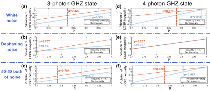
Figure 5: Comparison of the violation of the inequalities of inequalities Eq. (1) and Eq. (14) (for $N=4$) of Ref. [25] (in blue) with our improved inequalities (1) and (2) reported in the main paper (in red), with noisy GHZ state in the case of the 3-photon GHZ state (a-c) and the 4-photon GHZ state (d-f). For plots (a), (d), we adopt a white noise model ($k=0$). For plots (b), (e), we adopt a dephasing noise model ($k=1$). For plots (c), (f), we adopt a mixed noise model ($k=0.5$). Red lines represent the eventual violation of the inequalities Eq. (1) and Eq. (2), the violation threshold is indicated by a red dotted line. Blue lines represent the eventual violation of the main text inequalities Eq. (1) and Eq. (14) (for $N=4$) of Ref. [25], the violation threshold is indicated by a blue dotted line. All inequalities are rescaled by a constant such that the violation is obtained for positive values.

Appendix D $N$-party inequality

We derive analytically an inequality for any $N$ parties that is robust to noise. We take the two games in Reference [25] (we use the same notation),

$$I_{\textsf{Bell}}^{\tilde{C}_{1}{=}1}\coloneqq \langle A_{0}B_{0}\rangle_{\tilde{C}_{1}{=}1}+\langle A_{0}B_{1}\rangle_{\tilde{C}_{1}{=}1}+\langle A_{1}B_{0}\rangle_{\tilde{C}_{1}{=}1}-\langle A_{1}B_{1}\rangle_{\tilde{C}_{1}{=}1}\,,$$ (12)

and

$$I_{{\textsf{Same}}_{N}}\coloneqq\langle A_{0}B_{2}\rangle+ \langle B_{2}C_{0[1]}\rangle+\langle C_{0[1]}C_{0[2]}\rangle+[\dots]+\langle C_{0[N-3]}C_{0[N-2]}\rangle\,.$$ (13)

We then take Eq. 15 from Reference [25] (which reformulates Theorem 1 of Ref. [47, Eq. (11)]),

$$I_{{\textsf{Bell}}}^{\tilde{C}^{1}_{1}{=}1}\circ\{A^{1}B^{1}\}+2\langle A_{0}^{1}C_{0[N-2]}^{2}\rangle_{\tilde{C}^{1}_{1}{=}1}\leq 4\,.$$ (14)

We can obtain an inequality that is more robust to noise by observing that the Bell inequality still holds when conditioning the CHSH inequality upon the collectives of Charlies. i.e., if we define

$$I_{\textsf{Bell}}^{\tilde{C}_{1}{=}-1}\coloneqq \langle A_{0}B_{1}\rangle_{\tilde{C}_{1}{=}-1}+\langle A_{0}B_{0}\rangle_{\tilde{C}_{1}{=}-1}+\langle A_{1}B_{1}\rangle_{\tilde{C}_{1}{=}-1}-\langle A_{1}B_{0}\rangle_{\tilde{C}_{1}{=}-1}\,,$$ (15)

then Eq. 14 implies that the following convex combination also holds,

$$\frac{1-\langle\tilde{C}_{1}\rangle}{2}I_{{\textsf{Bell}}}^{\tilde{C}^{1}_{1}{=}-1}\circ\{A^{1}B^{1}\}+\frac{1+\langle\tilde{C}_{1}\rangle}{2}I_{{\textsf{Bell}}}^{\tilde{C}^{1}_{1}{=}1}\circ\{A^{1}B^{1}\}+2\langle A_{0}^{1}C_{0[N-2]}^{2}\rangle\leq 4\,.$$ (16)

We combine Eq. 14 with the following equation (Eq. 20 from Reference [25]),

$$\langle A^{2}_{0}C^{2}_{0[N-2]}\rangle\geq I_{\textsf{Same}}\circ\{A^{2}B^{2}C^{2}_{[0]}\dots C^{2}_{[N-2]}\}-N+2\,,$$ (17)

to obtain the following noise-robust inequality

$$\frac{1-\langle\tilde{C}_{1}\rangle}{2}I_{{\textsf{Bell}}}^{\tilde{C}^{1}_{1}{=}-1}\circ\{A^{1}B^{1}\}+\frac{1+\langle\tilde{C}_{1}\rangle}{2}I_{{\textsf{Bell}}}^{\tilde{C}^{1}_{1}{=}1}\circ\{A^{1}B^{1}\}+2I_{\textsf{Same}}\circ\{A^{2}B^{2}C^{2}_{[0]}\dots C^{2}_{[N-2]}\}\leq 2N\,.$$ (18)

This inequality is violated up to $2\sqrt{2}+2(N-1)$ with the $\left|\textrm{GHZ}_{N}\right\rangle$ states when Alice and Bob do, respectively, the measurements $\{\sigma_{Z},\sigma_{X}\}$ and $\{\frac{\sigma_{X}+\sigma_{Z}}{\sqrt{2}},\frac{-\sigma_{X}+\sigma_{Z}}{\sqrt{2}},\sigma_{Z}\}$, and all other players (i.e. the Charlies) measure following $\{\sigma_{Z},\sigma_{X}\}$.

Using the white-noise model of Eq. 10, we obtain a violation down to $p>\frac{n}{n-1+\sqrt{2}}$, while using the dephasing-plus-white-noise model of Eq. 11 results in a violation for the regime $p>\frac{k+2N(1-k)}{2\sqrt{2}-2(1+kN)+k+2N}$.

For $N=5$, this implies noise robustness of $p>\frac{5}{4+\sqrt{2}}\approx 0.923$ for the white noise model, which correspond to minimal fidelity requirements of $f\approx 0.926$. Considering the experimentally more realistic case of $k=0.5$, we obtain a noise robustness of $p>\frac{5.5}{3.5+2\sqrt{2}}\approx 0.869$, which correspond to minimal fidelity requirements of $f\approx 0.873$. This fidelity bound is on the edge of what can be achieved with current state-of-the-art multi-photon technologies [48, 49], which makes the observation of a violation challenging. Moreover, this would require very low counting rates to keep preserve the high fidelity of the source.

References

- Bell [1964] J. S. Bell, “On the Einstein-Podolsky-Rosen paradox,” Physics 1, 195 (1964).
- Spekkens [2007] R. W. Spekkens, “Evidence for the epistemic view of quantum states: A toy theory,” Phys. Rev. A 75, 032110 (2007).
- Popescu and Rohrlich [1994] S. Popescu and D. Rohrlich, “Quantum Nonlocality as an Axiom,” Found. Phys. 24, 379 (1994).
- Page [2005] D. N. Page, “Hawking radiation and black hole thermodynamics,” New J. Phys. 7, 203–203 (2005).
- Carlip [2001] S. Carlip, “Quantum gravity: a progress report,” Rep. Prog. Phys. 64, 885 (2001).
- Hardy [2019] L. Hardy, “Implementation of the quantum equivalence principle,” (2019), arXiv:1903.01289 [quant-ph] .
- Smith and Ahmadi [2019] A. R. H. Smith and M. Ahmadi, “Quantizing time: Interacting clocks and systems,” Quantum 3, 160 (2019).
- Galley et al. [2021] T. D. Galley, F. Giacomini, and J. H. Selby, “A no-go theorem on the nature of the gravitational field beyond quantum theory,” (2021), arXiv:2012.01441 [quant-ph] .
- Brunner et al. [2014] N. Brunner, D. Cavalcanti, S. Pironio, V. Scarani, and S. Wehner, “Bell nonlocality,” Rev. Mod. Phys. 86, 419 (2014).
- Bell [1966] J. S. Bell, “On the Problem of Hidden Variables in Quantum Mechanics,” Rev. Mod. Phys. 38, 447 (1966).
- Clauser et al. [1969] J. F. Clauser, M. A. Horne, A. Shimony, and R. A. Holt, “Proposed Experiment to Test Local Hidden-Variable Theories,” Phys. Rev. Lett. 23, 880 (1969).
- Freedman and Clauser [1972] S. J. Freedman and J. F. Clauser, “Experimental Test of Local Hidden-Variable Theories,” Phys. Rev. Lett. 28, 938 (1972).
- Aspect et al. [1981] A. Aspect, P. Grangier, and G. Roger, “Experimental Tests of Realistic Local Theories via Bell’s Theorem,” Phys. Rev. Lett. 47, 460 (1981).
- Tittel et al. [1998] W. Tittel, J. Brendel, H. Zbinden, and N. Gisin, “Violation of Bell Inequalities by Photons More Than 10 km Apart,” Phys. Rev. Lett. 81, 3563 (1998).
- Hensen et al. [2015] B. Hensen et al., “Loophole-free Bell inequality violation using electron spins separated by 1.3 kilometres,” Nature 526, 682 (2015).
- Shalm et al. [2015] L. K. Shalm et al., “Strong Loophole-Free Test of Local Realism,” Phys. Rev. Lett. 115, 250402 (2015).
- Giustina et al. [2015] M. Giustina et al., “Significant-Loophole-Free Test of Bell’s Theorem with Entangled Photons,” Phys. Rev. Lett. 115, 250401 (2015).
- Rosenfeld et al. [2017] W. Rosenfeld, D. Burchardt, R. Garthoff, K. Redeker, N. Ortegel, M. Rau, and H. Weinfurter, “Event-Ready Bell Test Using Entangled Atoms Simultaneously Closing Detection and Locality Loopholes,” Phys. Rev. Lett. 119, 010402 (2017).
- Li et al. [2018] M.-H. Li, C. Wu, Y. Zhang, W.-Z. Liu, B. Bai, Y. Liu, W. Zhang, Q. Zhao, H. Li, Z. Wang, L. You, W. J. Munro, J. Yin, J. Zhang, C.-Z. Peng, X. Ma, Q. Zhang, J. Fan, and J.-W. Pan, “Test of local realism into the past without detection and locality loopholes,” Phys. Rev. Lett. 121, 080404 (2018).
- Navascués et al. [2020] M. Navascués, E. Wolfe, D. Rosset, and A. Pozas-Kerstjens, “Genuine Network Multipartite Entanglement,” Phys. Rev. Lett. 125, 240505 (2020).
- Greenberger et al. [1990] D. M. Greenberger, M. A. Horne, A. Shimony, and A. Zeilinger, “Bell’s theorem without inequalities,” Am. J. Phys. 58, 1131 (1990).
- Barrett et al. [2005a] J. Barrett, N. Linden, S. Massar, S. Pironio, S. Popescu, and D. Roberts, “Nonlocal correlations as an information-theoretic resource,” Phys. Rev. A 71, 022101 (2005a).
- Contreras-Tejada et al. [2021] P. Contreras-Tejada, C. Palazuelos, and J. I. de Vicente, “Genuine multipartite nonlocality is intrinsic to quantum networks,” Physical Review Letters 126, 10.1103/physrevlett.126.040501 (2021).
- Coiteux-Roy et al. [2021a] X. Coiteux-Roy, E. Wolfe, and M.-O. Renou, “No Bipartite-Nonlocal Causal Theory Can Explain Nature’s Correlations,” Phys. Rev. Lett. 127, 200401 (2021a).
- Coiteux-Roy et al. [2021b] X. Coiteux-Roy, E. Wolfe, and M.-O. Renou, “Any Physical Theory of Nature Must Be Boundlessly Multipartite Nonlocal ,” Phys. Rev. A 104, 052207 (2021b).
- Wolfe et al. [2019] E. Wolfe, R. W. Spekkens, and T. Fritz, “The Inflation Technique for Causal Inference with Latent Variables,” J. Causal Inference 7, 0020 (2019).
- Gisin et al. [2020] N. Gisin, J.-D. Bancal, Y. Cai, P. Remy, A. Tavakoli, E. Z. Cruzeiro, S. Popescu, and N. Brunner, “Constraints on nonlocality in networks from no-signaling and independence,” Nature Comm. 11, 2378 (2020).
- Bancal and Gisin [2021] J.-D. Bancal and N. Gisin, “Non-Local Boxes for Networks,” arXiv:2102.03597 (2021).
- Beigi and Renou [2021] S. Beigi and M.-O. Renou, “Covariance Decomposition as a Universal Limit on Correlations in Networks,” arXiv:2103.14840 (2021).
- Pironio [2021] S. Pironio, “In Preparation,” (2021).
- Zhang et al. [2015] C. Zhang, Y.-F. Huang, Z. Wang, B.-H. Liu, C.-F. Li, and G.-C. Guo, “Experimental Greenberger-Horne-Zeilinger-Type Six-Photon Quantum Nonlocality,” Phys. Rev. Lett. 115, 260402 (2015).
- Wang et al. [2016] X.-L. Wang, L.-K. Chen, W. Li, H.-L. Huang, C. Liu, C. Chen, Y.-H. Luo, Z.-E. Su, D. Wu, Z.-D. Li, H. Lu, Y. Hu, X. Jiang, C.-Z. Peng, L. Li, N.-L. Liu, Y.-A. Chen, C.-Y. Lu, and J.-W. Pan, “Experimental Ten-Photon Entanglement,” Phys. Rev. Lett. 117, 210502 (2016).
- Erven et al. [2014] C. Erven, E. Meyer-Scott, K. Fisher, J. Lavoie, B. L. Higgins, Z. Yan, C. J. Pugh, J.-P. Bourgoin, R. Prevedel, L. K. Shalm, L. Richards, N. Gigov, R. Laflamme, G. Weihs, T. Jennewein, and K. J. Resch, “Experimental three-photon quantum nonlocality under strict locality conditions,” Nature Photonics 8, 292 (2014).
- Hamel et al. [2014] D. R. Hamel, L. K. Shalm, H. Hübel, A. J. Miller, F. Marsili, V. B. Verma, R. P. Mirin, S. W. Nam, K. J. Resch, and T. Jennewein, “Direct generation of three-photon polarization entanglement,” Nature Photonics 8, 801–807 (2014).
- Seevinck and Uffink [2001] M. Seevinck and J. Uffink, “Sufficient conditions for three-particle entanglement and their tests in recent experiments,” Phys. Rev. A 65, 012107 (2001).
- Svetlichny [1987] G. Svetlichny, “Distinguishing three-body from two-body nonseparability by a Bell-type inequality,” Phys. Rev. D 35, 3066 (1987).
- Tavakoli et al. [2021] A. Tavakoli, A. Pozas-Kerstjens, M.-X. Luo, and M.-O. Renou, “Bell nonlocality in networks,” arXiv:2104.10700 (2021).
- Fritz [2012] T. Fritz, “Beyond Bell’s theorem: correlation scenarios,” New J. Phys. 14, 103001 (2012).
- Branciard et al. [2010] C. Branciard, N. Gisin, and S. Pironio, “Characterizing the Nonlocal Correlations Created via Entanglement Swapping,” Phys. Rev. Lett. 104, 170401 (2010).
- Renou et al. [2019] M.-O. Renou, E. Bäumer, S. Boreiri, N. Brunner, N. Gisin, and S. Beigi, “Genuine Quantum Nonlocality in the Triangle Network,” Phys. Rev. Lett. 123, 140401 (2019).
- Barrett et al. [2005b] J. Barrett, N. Linden, S. Massar, S. Pironio, S. Popescu, and D. Roberts, “Nonlocal correlations as an information-theoretic resource,” Phys. Rev. A 71, 022101 (2005b).
- Gallego et al. [2012] R. Gallego, L. E. Würflinger, A. Acín, and M. Navascués, “Operational framework for nonlocality,” Phys. Rev. Lett. 109, 070401 (2012).
- Mao et al. [2022] Y.-L. Mao, Z.-D. Li, S. Yu, and J. Fan, “Test of genuine multipartite nonlocality in network,” (2022), arXiv:2201.12753 [quant-ph] .
- Gonda and Spekkens [2021] T. Gonda and R. W. Spekkens, “Monotones in General Resource Theories,” (2021), arXiv:1912.07085 [quant-ph] .
- Lancia and Serafini [2017] G. Lancia and P. Serafini, “Linear Programming,” in EURO Advanced Tutorials on Operational Research (Springer International Publishing, 2017) pp. 33–41.
- Wolfe and Yelin [2012] E. Wolfe and S. F. Yelin, “Quantum bounds for inequalities involving marginal expectation values,” Phys. Rev. A 86, 012123 (2012).
- Augusiak et al. [2014] R. Augusiak, M. Demianowicz, M. Pawłowski, J. Tura, and A. Acín, “Elemental and tight monogamy relations in nonsignaling theories,” Phys. Rev. A 90, 052323 (2014).
- Zhang et al. [2019] C. Zhang, T. R. Bromley, Y.-F. Huang, H. Cao, W.-M. Lv, B.-H. Liu, C.-F. Li, G.-C. Guo, M. Cianciaruso, and G. Adesso, “Demonstrating quantum coherence and metrology that is resilient to transversal noise,” Phys. Rev. Lett. 123, 180504 (2019).
- Li et al. [2020] Z.-D. Li, X.-F. Yin, Z. Wang, L.-Z. Liu, R. Zhang, Y.-Z. Zhang, X. Jiang, J. Zhang, L. Li, N.-L. Liu, et al., “Photonic realization of quantum resetting,” Optica 7, 766 (2020).
oneΔ