No-Regret Learning in Time-Varying Zero-Sum Games

Abstract

Learning from repeated play in a fixed two-player zero-sum game is a classic problem in game theory and online learning. We consider a variant of this problem where the game payoff matrix changes over time, possibly in an adversarial manner. We first present three performance measures to guide the algorithmic design for this problem: 1) the well-studied individual regret, 2) an extension of duality gap, and 3) a new measure called dynamic Nash Equilibrium regret, which quantifies the cumulative difference between the player’s payoff and the minimax game value. Next, we develop a single parameter-free algorithm that simultaneously enjoys favorable guarantees under all these three performance measures. These guarantees are adaptive to different non-stationarity measures of the payoff matrices and, importantly, recover the best known results when the payoff matrix is fixed. Our algorithm is based on a two-layer structure with a meta-algorithm learning over a group of black-box base-learners satisfying a certain property, along with several novel ingredients specifically designed for the time-varying game setting. Empirical results further validate the effectiveness of our algorithm.

1 Introduction

Repeated play in a fixed two-player zero-sum game, a fundamental problem in the interaction between game theory and online learning, has been extensively studied in recent decades. In particular, many efforts have been devoted to designing online algorithms such that both players achieve small individual regret (that is, difference between one’s cumulative payoff and that of the best fixed action) while at the same time the dynamics of the players’ strategy leads to a Nash equilibrium, a pair of strategies that neither player has incentive to deviate from; see for example (Freund & Schapire, 1999; Rakhlin & Sridharan, 2013; Daskalakis et al., 2015; Syrgkanis et al., 2015; Chen & Peng, 2020; Wei et al., 2021; Hsieh et al., 2021; Daskalakis et al., 2021).

In contrast to this large body of studies for learning over a fixed zero-sum game, repeated play over a sequence of time-varying games, the focus of this paper and a ubiquitous scenario in practice, is much less explored. While minimizing individual regret still makes perfect sense in this case, it is not immediately clear what other desirable game-theoretic guarantees are that generalize the concept of approaching a Nash equilibrium when the game is fixed. As far as we know, Cardoso et al. (2019) are the first to explicitly consider this problem. They proposed the notion of Nash-Equilibrium regret (NE-regret) as the performance measure, which quantifies the difference between the learners’ cumulative payoff and the minimax value of the cumulative payoff matrix. The authors proposed an algorithm with $\widetilde{\mathcal{O}}(\sqrt{T})$ NE-regret after $T$ rounds of play and, importantly, proved that no algorithm can simultaneously achieve sublinear NE-regret and sublinear individual regret for both players.

Our work starts by questioning whether the NE-regret of (Cardoso et al., 2019) is indeed a good performance measure for the problem of learning in time-varying games, especially given its incompatibility with the arguably most standard goal of having small individual regret. We then discover that measuring performance with NE-regret can in fact be highly unreasonable: we show an example (in Section 3) where even the two players perform perfectly (in the sense that they play the corresponding Nash equilibrium in every round), the resulting NE-regret is still linear in $T$!

Table 1: Summary of our results. The first column indicates the three performance measures considered in this work. The second column presents our main results for a sequence of time-varying payoff matrices $\{A_{t}\}_{t=1}^{T}$, and notably all results are simultaneously achieved by one single parameter-free algorithm. These guarantees are expressed in terms of three different (unknown) non-stationarity measures of the payoff matrices: $P_{T},V_{T}$, and $W_{T}$, all of which are $\Theta(T)$ in the worst-case and zero in the stationary case (when $A_{t}=A$ for all $t\in[T]$); see Section 3 for definitions. Additionally, for duality gap we use notation $Q_{T}$ as a shorthand for $V_{T}+\min\{P_{T},W_{T}\}$. Substituting all non-stationarity measures with zero leads to our corollaries for the stationary case shown in the third column, which match the state-of-the-art for all three performance measures (up to logarithmic factors) as shown in the last column.

Measure	Time-Varying Game ($\{A_{t}\}_{t=1}^{T}$, general)	Stationary Game ($A_{t}=A$, fixed)
Individual Regret	$\widetilde{\mathcal{O}}\big{(}\sqrt{1+V_{T}+\min\{P_{T},W_{T}\}}\big{)}$	$\widetilde{\mathcal{O}}(1)$	$\mathcal{O}(1)$
	[Theorem 4]	[Corollary 5]	(Hsieh et al., 2021)
Dynamic NE-Regret	$\widetilde{\mathcal{O}}\big{(}\min\{\sqrt{(1+V_{T})(1+P_{T})}+P_{T},1+W_{T}\}\big{)}$	$\widetilde{\mathcal{O}}(1)$	$\mathcal{O}(1)$
	[Theorem 6]	[Corollary 7]	(Hsieh et al., 2021)
Duality Gap	$\widetilde{\mathcal{O}}\big{(}\min\{T^{\frac{3}{4}}(1+Q_{T})^{\frac{1}{4}},T^{\frac{1}{2}}(1+Q_{T}^{\frac{3}{2}}+P_{T}Q_{T})^{\frac{1}{2}}\}\big{)}$	$\widetilde{\mathcal{O}}(\sqrt{T})$	$\mathcal{O}(\sqrt{T})$
	[Theorem 8]	[Corollary 9]	(Wei et al., 2021)

Motivated by this observation, we revisit the basic problem of how to measure the algorithm’s performance in such a time-varying game setting. Concretely, we consider three performance measures that we believe are appropriate and natural: 1) the standard individual regret; 2) the direct generalization of cumulative duality gap from a fixed game to a varying game; and 3) a new measure called dynamic NE-regret, which quantifies the difference between the learner’s cumulative payoff and the cumulative minimax game value (instead of the minimax value of the cumulative payoff matrix, as in NE-regret). We argue that dynamic NE-regret is a better measure compared to NE-regret: first, in the earlier example where both players play perfectly in each round using the corresponding Nash equilibrium, their dynamic NE-regret is exactly zero (while their NE-regret can be linear in $T$); second, having small dynamic NE-regret does not prevent one from enjoying small individual regret or duality gap (as will become clear soon).

With these performance measures in mind, our main contribution is to develop one single parameter-free algorithm that simultaneously enjoys favorable guarantees under all measures. These guarantees are adaptive to some unknown non-stationarity measures of the payoff matrices — naturally, the bounds worsen as the non-stationarity becomes larger. More specifically, the individual regret is always at most $\widetilde{\mathcal{O}}(\sqrt{T})$, the well-known worst-case bound, but could be much smaller if the non-stationarity measures are sublinear; on the other hand, the duality gap and dynamic NE-regret are sublinear as long as the non-stationarity measures are sublinear. In the special case of a fixed payoff matrix, all non-stationarity measures become zero and our results immediately recover the state-of-the-art results (up to logarithmic factors); see Table 1 for details. Notice that the best known results for a fixed game are not necessarily achieved by the same algorithm, while again, our results are all achieved by one adaptive algorithm. We also conduct empirical studies to further support our theoretical findings (Appendix H).

Techniques.   For a fixed game, Syrgkanis et al. (2015) proposed the “Regret bounded by Variation in Utilities” (RVU) property as the key condition for an algorithm to achieve good performance. On the other hand, one of the key tools for achieving our results is to ensure a small gap between each player’s cumulative payoff and that of a sequence of changing comparators, known as dynamic regret in the literature (Zinkevich, 2003). Therefore, our first step is to generalize the RVU property to “Dynamic Regret bounded by Variation in Utilities” (DRVU) property, and to show that many existing algorithms indeed satisfy DRVU.

Furthermore, to achieve strong guarantees for all performance measures without any prior knowledge, we also need to deploy a two-layer structure, with a meta-algorithm learning over and combining decisions of a group of base-learners, each of which satisfies the DRVU property but uses a different step size. Although such a framework has been used in many prior works in online learning (see for example the latest advances (Chen et al., 2021) and references therein), several new ingredients are required to achieve our results. First, when updating the meta-algorithm, a correction term related to the stability of each base-algorithm is injected into the loss for the corresponding base-algorithm, which plays a key role in the analysis. More specifically, we show (in Lemma 10) an explicit bound for the stability of the meta-algorithm’s decisions, whose proof requires a careful analysis using the correction terms above and the unique game structure. Second, we also introduce a set of additional “dummy” base-algorithms that always play some fixed action. This plays a key role in controlling the dynamics of the base-learners’ outputs and turns out to be critical when bounding the duality gap.

Related Work.   Two-player zero-sum game is one of the most fundamental problems in game theory, whose studies date back to the seminal work of von Neumann (1928). Freund & Schapire (1999) discovered the profound connections between zero-sum games and no-regret online learning, and since then there have been extensive studies on designing no-regret algorithms to solve games in the stationary setting (Rakhlin & Sridharan, 2013; Daskalakis et al., 2015; Syrgkanis et al., 2015; Chen & Peng, 2020; Wei et al., 2021; Daskalakis et al., 2021). We refer the reader to (Daskalakis et al., 2021) for a more thorough discussion on the literature. Several recent works start considering the problem of learning over a sequence of non-stationary payoffs under different structures, including zero-sum matrix games (Cardoso et al., 2019; Fiez et al., 2021), convex-concave games (Roy et al., 2019) and strongly monotone games (Duvocelle et al., 2021). For zero-sum games, (Fiez et al., 2021) focuses on the periodic case and proves divergence results for a class of learning algorithms; (Cardoso et al., 2019) is the closest to our work, but as mentioned, we argue that their proposed measure (NE-regret) is not always appropriate (see Section 3.1).

Organization.  We formally introduce the problem in Section 2, then present the performance measures in Section 3 and our algorithm in Section 4. Next, we provide theoretical guarantees in Section 5, and conclude in Section 6.

2 Problem Setup and Notations

We consider the following problem of two players (called $x$-player and $y$-player) repeatedly playing a zero-sum game for $T$ rounds, with $m$ fixed actions for $x$-player and $n$ fixed actions for $y$-player. At each round $t\in[T]\triangleq\{1,\ldots,T\}$, the environment first chooses a payoff matrix $A_{t}\in[-1,1]^{m\times n}$, whose $(i,j)$ entry denotes the loss/reward for $x$-player/$y$-player when they play action $i$ and action $j$ respectively. Without knowing $A_{t}$, $x$-player ($y$-player) decides her own mixed strategy (that is, a distribution over actions) $x_{t}\in\Delta_{m}$ ($y_{t}\in\Delta_{n}$), where $\Delta_{k}$ denotes the probability simplex $\Delta_{k}=\{u\in\mathbb{R}_{\geq 0}^{k}\mid\sum_{i=1}^{k}u_{i}=1\}$. At the end of this round, $x$-player suffers expected loss $x_{t}^{\top}A_{t}y_{t}$ and observes the loss vector $A_{t}y_{t}$, while $y$-player receives the expected reward $x_{t}^{\top}A_{t}y_{t}$ and observes the reward vector $x_{t}^{\top}A_{t}$. Note that neither player observes the matrix $A_{t}$ itself.

When $A_{t}$ is fixed for all $t$, this exactly recovers the standard stationary setting considered in for example (Syrgkanis et al., 2015). Having a time-varying $A_{t}$ allows us to capture various possible sources of non-stationarity in the environment. In fact, $A_{t}$ can even be decided by an adaptive adversary who makes the decision knowing the players’ algorithm and their decisions in earlier rounds. Our setting is almost the same as (Cardoso et al., 2019), except that the feedback they consider is either the entire matrix $A_{t}$ (stronger than ours) or just one entry of $A_{t}$ sampled according to $(x_{t},y_{t})$ (weaker than ours).

For each game matrix $A_{t}$, define the set of minimax strategies for $x$-player as ${\mathcal{X}}_{t}^{*}=\operatorname*{argmin}_{x\in\Delta_{m}}\min_{y\in\Delta_{n}}x^{\top}A_{t}y$ and similarly the set of maximin strategies for $y$-player as ${\mathcal{Y}}_{t}^{*}=\operatorname*{argmax}_{y\in\Delta_{n}}\min_{x\in\Delta_{m}}x^{\top}A_{t}y$. It is well-known that any pair $(x_{t}^{*},y_{t}^{*})\in{\mathcal{X}}_{t}^{*}\times{\mathcal{Y}}_{t}^{*}$ forms a Nash equilibrium of $A_{t}$ with the following saddle-point property: $x_{t}^{*\top}A_{t}y\leq x_{t}^{*\top}A_{t}y_{t}^{*}\leq x^{\top}A_{t}y_{t}^{*}$ holds for any $x\in\Delta_{m}$ and $y\in\Delta_{n}$. Throughout the paper, $(x_{t}^{*},y_{t}^{*})$ denotes an arbitrary Nash equilibrium of $A_{t}$.

Notations.   For a real-valued matrix $A\in\mathbb{R}^{m\times n}$, its infinity norm is defined as $\|A\|_{\infty}\triangleq\max_{i,j}|A_{ij}|$. We use $\mathbf{1}_{N}$ and $\mathbf{0}_{N}$ to denote the all-one and all-zero vectors of length $N$. For conciseness, we often hide polynomial dependence on the size of the game (that is, $m$ and $n$) in the $\mathcal{O}(\cdot)$-notation. The $\widetilde{\mathcal{O}}(\cdot)$-notation further omits logarithmic dependence on $T$. We sometimes write $\min_{x\in\Delta_{m}}$ ($\min_{y\in\Delta_{n}}$) simply as $\min_{x}$ ($\min_{y}$) when there is no confusion.

3 How to Measure the Performance?

With the learning protocol specified, the next pressing question is to determine what the goal is when designing algorithms for the two players. When $A_{t}$ is fixed, most studies consider minimizing individual regret for each player and some form of convergence to a Nash equilibrium of the fixed game as the two primary goals. While minimizing individual regret is still naturally defined when $A_{t}$ is changing over time, it is less clear what other desirable game-theoretic guarantees are in this case. In Section 3.1, we formally discuss three performance measures that we think are reasonable for this problem. Then in Section 3.2, we further discuss how to measure the non-stationarity of the sequence $\{A_{t}\}_{1:T}$ that will play a role in how well the players can do under some of the performance measures.

3.1 Performance Measures

Individual Regret.  The first measure we consider is the standard individual regret. For $x$-player, this is defined as

$$\text{\rm Reg}_{T}^{x}\triangleq\sum_{t=1}^{T}x_{t}^{\top}A_{t}y_{t}-\min_{x\in\Delta_{m}}\sum_{t=1}^{T}x^{\top}A_{t}y_{t},$$ (1)

that is, the difference between her total loss and that of the best fixed strategy (assuming the same behavior from the opponent). Similarly, the regret for $y$-player is defined as $\text{\rm Reg}_{T}^{y}\triangleq\max_{y\in\Delta_{n}}\sum_{t=1}^{T}x_{t}^{\top}A_{t}y-\sum_{t=1}^{T}x_{t}^{\top}A_{t}y_{t}$. Achieving sublinear (in $T$) individual regret implies that on average each player performs almost as well as their best fixed strategy, and this is arguably the most standard and basic goal for online learning problems.

Duality Gap.   For a game matrix $A_{t}$, the duality gap of a pair of strategy $(x_{t},y_{t})$ is defined as $\max_{y\in\Delta_{n}}x_{t}^{\top}A_{t}y-\min_{x\in\Delta_{m}}x^{\top}A_{t}y_{t}$. It is always nonnegative since $\max_{y\in\Delta_{n}}x_{t}^{\top}A_{t}y\geq x_{t}^{\top}A_{t}y_{t}^{*}\geq x_{t}^{*\top}A_{t}y_{t}^{*}\geq x_{t}^{*\top}A_{t}y_{t}\geq\min_{x\in\Delta_{m}}x^{\top}A_{t}y_{t}$, and it is zero if and only if $(x_{t},y_{t})$ is a Nash equilibrium of $A_{t}$. Thus, the duality gap measures how close $(x_{t},y_{t})$ is to the equilibria in some sense. We thus naturally use the cumulative duality gap:

$$\text{\rm Dual-Gap}_{T}\triangleq\sum_{t=1}^{T}\Big{(}\max_{y\in\Delta_{n}}x_{t}^{\top}A_{t}y-\min_{x\in\Delta_{m}}x^{\top}A_{t}y_{t}\Big{)},$$ (2)

as another performance measure. When $A_{t}$ is fixed, this measure is considered in (Wei et al., 2021) for example.

Dynamic Nash Equilibrium (NE)-Regret.   Before introducing this last measure, we first review what Cardoso et al. (2019) proposed as the goal for this problem, that is, ensuring small Nash Equilibrium (NE)-regret, defined as

$$\text{\rm NE-Reg}_{T}\triangleq\Bigg{|}\sum_{t=1}^{T}x_{t}^{\top}A_{t}y_{t}-\min_{x\in\Delta_{m}}\max_{y\in\Delta_{n}}\sum_{t=1}^{T}x^{\top}A_{t}y\Bigg{|}.$$ (3)

In words, this is the difference between the cumulative loss of $x$-player (or equivalently the cumulative reward of $y$-player) and the minimax value of the cumulative payoff matrix ($\sum_{t=1}^{T}A_{t}$). While this might appear to be a reasonable generalization of individual regret for a central controller who decides $x_{t}$ and $y_{t}$ jointly, we argue below that this measure is in fact often inappropriate for two reasons.

The first reason is in fact already hinted in (Cardoso et al., 2019): they proved that no algorithm can always ensure sublinear NE-regret and simultaneously sublinear individual regret for both players. Given that minimizing individual regret selfishly is a natural impulse and the standard goal for each player, NE-regret can only make sense when both players are controlled by a centralized algorithm.

The second reason is perhaps more profound. Consider the following two-phase example: when $t\leq T/2$, $A_{t}={\scriptsize\begin{pmatrix}1&-1\\ -1&1\end{pmatrix}}$; when $t>T/2$, $A_{t}={\scriptsize\begin{pmatrix}1&-1\\ 1&-1\end{pmatrix}}$. It is straightforward to verify that: when $t\leq T/2$, the equilibrium for $A_{t}$ is the uniform distribution for both players, leading to game value $0$; when $t>T/2$, the equilibrium is such that $y$-player always picks the first column, leading to game value $1$; and the equilibrium for the cumulative game matrix $\sum_{t=1}^{T}A_{t}={\scriptsize\begin{pmatrix}T&-T\\ 0&0\end{pmatrix}}$ is $x$-player picking the second row while $y$-player picking the first column, leading to game value $0$. To sum up, even if both players play perfectly in each round using the corresponding equilibrium, their NE-regret is still $|T/2-0|=T/2$, which is a vacuous bound linear in $T$!

Motivated by the observations above, we propose a variant of NE-regret as the third performance measure, called dynamic NE-regret:

$$\text{\rm DynNE-Reg}_{T}\triangleq\Bigg{|}\sum_{t=1}^{T}x_{t}^{\top}A_{t}y_{t}-\sum_{t=1}^{T}\min_{x\in\Delta_{m}}\max_{y\in\Delta_{n}}x^{\top}A_{t}y\Bigg{|}.$$

Compared to NE-regret, here we move the minimax operation inside the summation, making it the cumulative difference between $x$-player’s loss and the minimax game value in each round. In other words, similarly to duality gap, dynamic NE-regret provides yet another way to measure in each round, how close $(x_{t},y_{t})$ is to the equilibria of $A_{t}$ from the game value perspective.

The connection between NE-regret and Dynamic NE-regret is on the surface analogous to that between standard regret and dynamic regret (Zinkevich, 2003) (see Appendix B.1 for definitions and more related discussions). However, while dynamic regret is always no less than standard regret, Dynamic NE-regret could be smaller than NE-regret — simply consider our earlier two-phase example: the perfect players (who always play an equilibrium) clearly have $0$ dynamic NE-regret, but their NE-regret is $T/2$ as discussed. This example also shows that dynamic NE-regret is more reasonable compared to NE-regret. Moreover, as will become clear soon, dynamic NE-regret is compatible with individual regret (and also duality gap), in the sense there are algorithms that provably perform well under all these measures.

We conclude this section with the following two remarks.

Remark 1 (Comparisons of the three measures).

Both individual regret and dynamic NE-regret are bounded by duality gap (see proofs in Appendix B.2), but the latter could be much larger. On the other hand, individual regret and dynamic NE-regret are generally incomparable.

Remark 2 (Other possibilities).

The three measures we consider are by no mean the only possibilities. Another reasonable one is the tracking error $\sum_{t=1}^{T}(\lVert x_{t}-x_{t}^{*}\rVert_{1}+\lVert y_{t}-y_{t}^{*}\rVert_{1})$ that directly measures the distance between $(x_{t},y_{t})$ and the equilibrium $(x_{t}^{*},y_{t}^{*})$ (assuming unique equilibrium for simplicity). This is considered in (Roy et al., 2019; Balasubramanian & Ghadimi, 2021) (for different problems). However, tracking error bounds are in fact not well studied even when $A_{t}$ is fixed — the best known results still depend on some problem-dependent constant that can be arbitrarily large (Daskalakis & Panageas, 2019; Wei et al., 2021). Deriving tracking error bounds in our setting is thus beyond the scope of this paper. Note that in many optimization studies, one often only cares about finding a point that is close to the optimal solution in terms of their function value instead of their absolute distance. Our dynamic NE-regret and duality gap are both in this same sprite by looking at the game value instead of the actual distance as in tracking error.

3.2 Non-stationarity Measures

For duality gap and dynamic NE-regret, it is not difficult to see that if $A_{t}$ changes drastically over time, then no meaningful guarantees are possible. This is similar to dynamic regret in standard online learning problems, where guarantees are always expressed in terms of some non-stationarity measure of the environment and are meaningful only when the non-stationarity is reasonably small. In our setting, we consider the following three different ways to measure non-stationarity of the sequence $\{A_{t}\}_{t=1}^{T}$.

Variation of Nash Equilibria.  Recall the notation ${\mathcal{X}}_{t}^{*}\times{\mathcal{Y}}_{t}^{*}$, the set of Nash equilibria for matrix $A_{t}$. Define the variation of Nash equilibria as:

$$P_{T}\triangleq\min_{\forall t,(x_{t}^{*},y_{t}^{*})\in{\mathcal{X}}_{t}^{*}\times{\mathcal{Y}}_{t}^{*}}\sum_{t=2}^{T}\left(\|x_{t}^{*}-x_{t-1}^{*}\|_{1}+\|y_{t}^{*}-y_{t-1}^{*}\|_{1}\right),$$

which quantifies the drift of the Nash equilibria of the game matrices in $\ell_{1}$-norm.

Variation/Variance of Game Matrices.  The path-length variation and the variance of $\{A_{t}\}_{t=1}^{T}$ are respectively defined as

$$V_{T}\triangleq\sum_{t=2}^{T}\|A_{t}-A_{t-1}\|_{\infty}^{2},~{}~{}~{}W_{T}\triangleq\sum_{t=1}^{T}\|A_{t}-\bar{A}\|_{\infty},$$

where $\bar{A}=\frac{1}{T}\sum_{t=1}^{T}A_{t}$ is the averaged game matrix.

Clearly, $P_{T}$, $V_{T}$, and $W_{T}$ are all $\Theta(T)$ in the worst case, and $0$ when $A_{t}$ is fixed over time. For dynamic regret and duality gap, the natural goal is to enjoy sublinear bounds whenever (some of) these non-stationarity measures are sublinear (which we indeed achieve).

We conclude by pointing out some connections between these non-stationarity measures. First, $V_{T}\leq 4W_{T}$ holds but the former could be much smaller. Second, $P_{T}$ is generally not comparable with $V_{T}$ and $W_{T}$, and there are examples where $P_{T}=0$ and $V_{T}=W_{T}=\Theta(T)$, or $P_{T}=\Theta(T)$ and $V_{T}=W_{T}=\mathcal{O}(1)$. We defer all details to Appendix B.

4 Proposed Algorithm

In this section, we present our proposed algorithm for time-varying games, which provably achieves favorable guarantees under all three performance measures. To illustrate the ideas behind our algorithm design, we first review how (Syrgkanis et al., 2015) achieves fast convergence results for a fixed game, followed by a detailed discussion on how to generalize their idea and overcome the difficulties brought by time-varying games. For conciseness, throughout the section we focus on the $x$-player; how the $y$-player should behave is completely symmetric.

For a fixed game $A_{t}=A$, Syrgkanis et al. (2015) proposed that each player should deploy an online learning algorithm that satisfies a specific property called “Regret bounded by Variation in Utilities” (RVU). More specifically, an online learning algorithm proposes $x_{t}\in\Delta_{m}$ at the beginning of round $t$, and then receives a loss vector $g_{t}\in\mathbb{R}^{m}$ and suffers loss $\left\langle{x_{t},g_{t}}\right\rangle$. Its regret against a comparator $u\in\Delta_{m}$ after $T$ rounds is naturally $\sum_{t=1}^{T}\left\langle{x_{t}-u,g_{t}}\right\rangle$, and the RVU property states that this should be bounded by $\alpha+\beta\sum_{t=2}^{T}\|g_{t}-g_{t-1}\|_{\infty}^{2}-\gamma\sum_{t=2}^{T}\|x_{t}-x_{t-1}\|_{1}^{2}$ for some parameters $\alpha,\beta,\gamma>0$. To see why RVU property is useful, consider $x$-player deploying such an algorithm with $g_{t}$ set to $A_{t}y_{t}=Ay_{t}$. Then her regret is further bounded as $\alpha+\beta\sum_{t=2}^{T}\lVert Ay_{t}-Ay_{t-1}\rVert_{\infty}^{2}-\gamma\sum_{t=2}^{T}\lVert x_{t}-x_{t-1}\rVert_{1}^{2}\leq\alpha+\beta\sum_{t=2}^{T}\lVert y_{t}-y_{t-1}\rVert_{1}^{2}-\gamma\sum_{t=2}^{T}\lVert x_{t}-x_{t-1}\rVert_{1}^{2}$. Therefore, as long as $y$-player also deploys the same algorithm, by symmetry, the sum of their regret is at most $\alpha+(\beta-\gamma)(\sum_{t=2}^{T}\lVert x_{t}-x_{t-1}\rVert_{1}^{2}+\sum_{t=2}^{T}\lVert y_{t}-y_{t-1}\rVert_{1}^{2})$, which can be simply bounded by (a constant) $\alpha$ as long as $\beta\leq\gamma$. Many useful guarantees can then be obtained as a corollary of the fact that the sum of regret is small.

In our setting where $A_{t}$ is changing over time, our first observation is that instead of the sum of the two players’ regret, what we need to control is the sum of their dynamic regret (Zinkevich, 2003), which plays an important role when deriving guarantees for all the three measures (including individual regret). Specifically, for an online learning algorithm producing $x_{t}$ and receiving $g_{t}$, its dynamic regret against a sequence of comparators $u_{1},\ldots,u_{T}\in\Delta_{m}$ is defined as $\sum_{t=1}^{T}\left\langle{x_{t}-u_{t},g_{t}}\right\rangle$. Generalizing RVU, we naturally introduce the following “Dynamic Regret bounded by Variation in Utilities” (DRVU) property.

Definition 3 (DRVU Property).

Denote by ${\mathcal{A}}(\eta)$ an online learning algorithm with a parameter $\eta>0$. We say that it satisfies the Dynamic Regret bounded by Variation in Utilities property (abbreviated as DRVU($\eta$)) with parameters $\alpha,\beta,\gamma>0$, if its dynamic regret $\sum_{t=1}^{T}\left\langle{x_{t}-u_{t},g_{t}}\right\rangle$ on any loss sequence $g_{1},\ldots,g_{T}$ with respect to any comparator sequence $u_{1},\ldots,u_{T}$ is bounded by

$$\frac{\alpha}{\eta}(1+P_{T}^{u})+\eta\beta\sum_{t=1}^{T}\|g_{t}-g_{t-1}\|_{\infty}^{2}-\frac{\gamma}{\eta}\sum_{t=2}^{T}\|x_{t}-x_{t-1}\|_{1}^{2},$$

where $P_{T}^{u}\triangleq\sum_{t=2}^{T}\lVert u_{t}-u_{t-1}\rVert_{1}$ is the path-length of the comparator sequence.

Compared to RVU, DRVU naturally replaces the first constant term in the regret bound with a term depending on the path-length of the comparator sequence. We also add another step size parameter $\eta$ (whose role will become clear soon). Recent studies in dynamic regret (Zhao et al., 2020, 2021) show that variants of optimistic Online Mirror Descent (such as Optimistic Gradient Descent and Optimistic Hedge) indeed satisfy DRVU with $\alpha,\beta,\gamma=\widetilde{\Theta}(1)$; see Appendix D for formal statements and proofs.

Now, if $x$-player deploys an algorithm satisfying DRVU and feeds it with loss vector $g_{t}=A_{t}y_{t}$ (and similarly $y$-player does the same), we can indeed prove a desired guarantee for each of the three performance measures. However, the tuning of $\eta$ will require the knowledge of the unknown parameters $P_{T},V_{T},W_{T}$ and, perhaps more importantly, be different for each different measures. To obtain an adaptive algorithm that performs well under all three measures without any prior knowledge, we further propose a two-layer structure with a meta-algorithm learning over and combining decisions of a set of base-learners, each of which satisfies DRVU($\eta$) but with a different step size $\eta$. While this idea of “learning over learning algorithms” is not new in online learning, we will discuss below what extra difficulties show up in our case and how we address them.

4.1 Base-learners

Define $N=\lfloor\frac{1}{2}\log_{2}T\rfloor+1$. Our algorithm maintains $N+m$ base-learners: for $i\in[N]$, the $i$-th base-learner is any algorithm that satisfies $\textsc{DRVU}(\eta_{i}^{x})$, where $\eta_{i}^{x}=\frac{2^{i-1}}{L\sqrt{T}}$ and

$$L=\max\big{\{}4,\sqrt{16c\beta},\sqrt{8c\beta/\gamma}\big{\}}$$ (4)

($\beta$ and $\gamma$ are the parameters from DRVU and $c=\widetilde{\mathcal{O}}(1)$ is a constant whose exact value can be found in the proof); the last $m$ base-learners are dummy learners, with the $(j+N)$-th one always outputting the basis vector $e_{j}\in\Delta_{m}$ (that is, always choosing the $j$-th action). We note that the dummy base-learners are important in controlling the duality gap (but not the other two measures). We let ${\mathcal{S}}_{x}\triangleq{\mathcal{S}}_{1,x}\cup{\mathcal{S}}_{2,x}$ with ${\mathcal{S}}_{1,x}=[N]$ and ${\mathcal{S}}_{2,x}=\{N+1,\ldots,N+m\}$ denote the set of indices of base-learners.

At round $t$, each base-learner $i$ submits her decision $x_{t,i}\in\Delta_{m}$ to the meta-algorithm, who decides the final decision $x_{t}$. Upon receiving the feedback $A_{t}y_{t}$, the meta-algorithm sends the same (as the loss vector $g_{t}$) to each base-learner $i\in{\mathcal{S}}_{1,x}$ (no updates needed for the dummy base-learners).

4.2 Meta-algorithm

With all the decisions $\{x_{t,i}\}_{i\in{\mathcal{S}}_{x}}$ collected from the base-learners, the meta-algorithm outputs the final decision $x_{t}=\sum_{i\in{\mathcal{S}}_{x}}p_{t,i}x_{t,i}$, where $p_{t}\in\Delta_{|{\mathcal{S}}_{x}|}$ is a distribution over the base-learners updated according to a version of Optimistic Online Gradient Descent (OOGD) (Rakhlin & Sridharan, 2013; Syrgkanis et al., 2015):

$$\begin{split}p_{t}&=\operatorname*{argmin}_{p\in\Delta_{|{\mathcal{S}}_{x}|}}\left\{\varepsilon_{t}^{x}\langle p,m_{t}^{x}\rangle+\|p-\widehat{p}_{t}\|_{2}^{2}\right\},\\ \widehat{p}_{t+1}&=\operatorname*{argmin}_{p\in\Delta_{|{\mathcal{S}}_{x}|}}\left\{\varepsilon_{t}^{x}\langle p,\ell_{t}^{x}\rangle+\|p-\widehat{p}_{t}\|_{2}^{2}\right\}.\end{split}$$ (5)

Here, $\varepsilon_{t}^{x}>0$ is a time-varying learning rate, $\{\widehat{p}_{t}\}_{t=1,2,\ldots}$ is an auxiliary sequence (starting with $\widehat{p}_{1}$ as the uniform distribution) updated via projected gradient descent using some loss vector sequence $\ell_{1}^{x},\ell_{2}^{x},\ldots\in\mathbb{R}^{|{\mathcal{S}}_{x}|}$, and $p_{t}$ is updated via projected gradient descent from the distribution $\widehat{p}_{t}$ and using a loss predictor $m_{t}^{x}\in\mathbb{R}^{|{\mathcal{S}}_{x}|}$. It remains to specify what $\ell_{t}^{x}$ and $m_{t}^{x}$ are (the tuning of the learning rate will be specified in the final algorithm).

Input: a base-algorithm $\mathcal{A}(\eta)$ satisfying DRVU($\eta$).

Initialize: a set of base-learners ${\mathcal{S}}_{x}$ as described in Section 4.1, $\widehat{p}_{1}=\frac{1}{|{\mathcal{S}}_{x}|}\mathbf{1}_{|{\mathcal{S}}_{x}|}$, learning rate $\varepsilon_{1}^{x}=\frac{1}{L}$ (c.f. Eq. (4)).

for $t=1,\dots,T$ do

       Receive $x_{t,i}\in\Delta_{m}$ from each base-learner $i\in{\mathcal{S}}_{x}$.

      Compute $m_{t}^{x}$ based on Eq. (7) and $p_{t}$ based on Eq. (5).

      Play the final decision $x_{t}=\sum_{i\in{\mathcal{S}}_{x}}p_{t,i}x_{t,i}$.

      Suffer loss $x_{t}^{\top}A_{t}y_{t}$ and observe the loss vector $A_{t}y_{t}$.

      Compute $\ell_{t}^{x}$ based on Eq. (6) and $\widehat{p}_{t+1}$ based on Eq. (5).

      Update $\varepsilon_{t+1}^{x}=\nicefrac{{1}}{{\sqrt{L^{2}+\sum_{s=2}^{t}\|A_{t}y_{t}-A_{t-1}y_{t-1}\|_{\infty}^{2}}}}$.

      Send $A_{t}y_{t}$ as the feedback to each base-learner.

end for

Algorithm 1 Algorithm for the $x$-player

Since base-learner $i$ predicts $x_{t,i}$ and receives loss vector $A_{t}y_{t}$, it is natural to set its loss $\ell_{t,i}^{x}$ as $x_{t,i}^{\top}A_{t}y_{t}$ from the meta-algorithm’s perspective. In light of standard OOGD, $m_{t}^{x}$ should then be set to $x_{t,i}^{\top}A_{t-1}y_{t-1}$, meaning that the last loss vector $A_{t-1}y_{t-1}$ is used to predict the current one (that is unknown yet when computing $p_{t}$). However, this setup leads to the following issue. When applying DRVU($\eta_{i}^{x}$) to this base-learner, we see that a negative term related to $\|x_{t,i}-x_{t-1,i}\|_{1}^{2}$ and a positive term related to $\|y_{t}-y_{t-1}\|_{1}^{2}$ arise (the latter is from $\|A_{t}y_{t}-A_{t-1}y_{t-1}\|_{\infty}^{2}\leq 2\lVert A_{t}-A_{t-1}\rVert_{\infty}^{2}+2\|y_{t}-y_{t-1}\|_{1}^{2}$, with the first term only related to the non-stationarity of game matrices). By symmetry, $y$-player contributes a positive term $\|x_{t}-x_{t-1}\|_{1}^{2}$, which now cannot be canceled by $\|x_{t,i}-x_{t-1,i}\|_{1}^{2}$, unlike the case with only one learner for each player discussed earlier.

To address this issue, we propose to add a stability correction term to both $\ell_{t}^{x}$ and $m_{t}^{x}$. Concretely, they are defined as $\ell_{1,i}^{x}=x_{1,i}^{\top}A_{1}y_{1}$ and $m_{1,i}^{x}=0,\forall i$, and for all $t\geq 2$:

$$\ell_{t,i}^{x}={} x_{t,i}^{\top}A_{t}y_{t}+\lambda\lVert x_{t,i}-x_{t-1,i}\rVert_{1}^{2},$$ (6)

$$m_{t,i}^{x}={} x_{t,i}^{\top}A_{t-1}y_{t-1}+\lambda\lVert x_{t,i}-x_{t-1,i}\rVert_{1}^{2},$$ (7)

where $\lambda=\frac{\gamma L}{2}$ ($\gamma$ is the parameter from DRVU). From a technical perspective, this introduces to the regret a negative term $\sum_{i\in{\mathcal{S}}_{x}}p_{t,i}\lVert x_{t,i}-x_{t-1,i}\rVert_{1}^{2}$, and a positive term $\lVert x_{t,i}-x_{t-1,i}\rVert_{1}^{2}$ which can be canceled by the aforementioned negative term from DRVU($\eta_{i}^{x}$). To see why the extra negative term is useful, notice that the troublesome term $\|x_{t}-x_{t-1}\|_{1}^{2}$ from DRVU($\eta_{i}^{x}$) can be bounded as

$$\lVert x_{t}-x_{t-1}\rVert_{1}^{2}=\left\lVert\sum_{i\in{\mathcal{S}}_{x}}p_{t,i}x_{t,i}-\sum_{i\in{\mathcal{S}}_{x}}p_{t-1,i}x_{t-1,i}\right\rVert_{1}^{2}$$

$$\leq 2\sum_{i\in{\mathcal{S}}_{x}}p_{t,i}\lVert x_{t,i}-x_{t-1,i}\rVert_{1}^{2}+2\lVert p_{t}-p_{t-1}\rVert_{1}^{2},$$

where the first term can exactly be canceled by the extra negative term introduced by the correction term, and the second term can in fact also be canceled in a standard way since the meta-algorithm itself can be shown to satisfy RVU. This explains the design of our correction terms from a technical level. Intuitively, injecting this correction term guides the meta-algorithm to bias toward the more stable base-learners, hence also stabilizing the final decision $x_{t}$.

We note that a similar technique was used in analyzing gradient-variation dynamic regret for online convex optimization (Zhao et al., 2021). Our approach is different from theirs in the sense that there is only one player in their setting and the correction term is used to cancel the additional gradient variation introduced by the variation of her own decision. In contrast, in our setting the correction term is used to cancel the opponent’s gradient variation.

To summarize, our final algorithm (for the $x$-player) is presented in Algorithm 1. We also include the symmetric version for the $y$-player in Algorithm 2 (Appendix A) for completeness. We emphasize again that this is a parameter-free algorithm that does not require any prior knowledge of the environment.

5 Theoretical Guarantees and Analysis

In this section, we first provide the guarantees of our algorithm under each of the three performance measures, and then highlight several key ideas in the analysis, with the full proofs deferred to Appendix E. Recall that our guarantees are all expressed in terms of the non-stationarity measures $P_{T}$, $V_{T}$, and $W_{T}$, defined in Section 3.2. Also, to avoid showing the cumbersome dependence on the DRVU parameters ($\alpha$, $\beta$, $\gamma$) in all our bounds, we will simply assume that they are all $\widetilde{\Theta}(1)$, which, as mentioned earlier and shown in Appendix D, is indeed the case for standard algorithms.

5.1 Performance Guarantees

We state our results for each performance measure separately below, but emphasize again that they hold simultaneously. First, we show the individual regret bound.

Theorem 4 (Individual Regret).

When the $x$-player uses Algorithm 1, irrespective of $y$-player’s strategies, we have

$$\text{\rm Reg}_{T}^{x}=\sum_{t=1}^{T}x_{t}^{\top}A_{t}y_{t}-\min_{x}\sum_{t=1}^{T}x^{\top}A_{t}y_{t}=\widetilde{\mathcal{O}}(\sqrt{T}).$$

Furthermore, if $x$-player follows Algorithm 1 and $y$-player follows Algorithm 2, then individual regret satisfies:

$$\max\left\{\text{\rm Reg}_{T}^{x},\text{\rm Reg}_{T}^{y}\right\}=\widetilde{\mathcal{O}}\Big{(}\sqrt{1+V_{T}+\min\{P_{T},W_{T}\}}\Big{)}.$$

The first statement of Theorem 4 provides a robustness guarantee for our algorithm — no matter how non-stationary the game matrices are and no matter how the opponent behaves, following our algorithm always ensures $\widetilde{\mathcal{O}}(\sqrt{T})$ individual regret, the standard worst-case regret bound. On the other hand, when both players follow our algorithm, their individual regret could be even smaller depending on the non-stationarity. In particular, as long as $V_{T}+\min\{P_{T},W_{T}\}=o(T)$ (that is, not the worst case scenario), our bound becomes $o(\sqrt{T})$. Also note that $P_{T}$ and $W_{T}$ are generally incomparable (see Appendix B), but our bound achieves the minimum of them, thus achieving the best of both worlds.

When the game matrix is fixed, we have $P_{T}=V_{T}=W_{T}=0$, immediately leading to the following corollary.

Corollary 5.

When $x$-player follows Algorithm 1 and $y$-player follows Algorithm 2, if $A_{t}=A$ for all $t\in[T]$, then $\max\left\{\text{\rm Reg}_{T}^{x},\text{\rm Reg}_{T}^{y}\right\}=\widetilde{\mathcal{O}}(1)$.

The best known individual regret bound for learning in a fixed two-player zero-sum game is $\mathcal{O}(1)$ (Hsieh et al., 2021). Our result matches theirs up to logarithmic factors.

The next theorem presents the dynamic NE-regret bound.

Theorem 6 (Dynamic NE-Regret).

When $x$-player follows Algorithm 1 and $y$-player follows Algorithm 2, we have the following dynamic NE-regret bound:

$$\text{\rm DynNE-Reg}_{T}=\left|\sum_{t=1}^{T}x_{t}^{\top}A_{t}y_{t}-\sum_{t=1}^{T}\min_{x\in\Delta_{m}}\max_{y\in\Delta_{n}}x^{\top}A_{t}y\right|$$

$$=\widetilde{\mathcal{O}}\big{(}\min\{\sqrt{(1+V_{T})(1+P_{T})}+P_{T},1+W_{T}\}\big{)}.$$

Similarly, our dynamic NE-regret bound is $o(T)$ as long as $P_{T}$ or $W_{T}$ is $o(T)$. When the game matrix is fixed, we again obtain the following direct corollary by noticing $P_{T}=V_{T}=W_{T}=0$ in this case.

Corollary 7.

When $x$-player follows Algorithm 1 and $y$-player follows Algorithm 2, if $A_{t}=A$ for all $t\in[T]$, then $\text{\rm DynNE-Reg}_{T}=\widetilde{\mathcal{O}}(1)$.

In fact, when the game is fixed, dynamic NE-regret degenerates to NE-regret of (Cardoso et al., 2019) as $\sum_{t=1}^{T}\min_{x}\max_{y}x^{\top}Ay=\min_{x}\max_{y}\sum_{t=1}^{T}x^{\top}Ay$. Their algorithm would achieve $\widetilde{\mathcal{O}}(\sqrt{T})$ (dynamic) NE-regret in this case. A better $\mathcal{O}(1)$ result is implicitly implied by the aforementioned work of Hsieh et al. (2021), as we show (in Lemma 17) that (dynamic) NE-regret is bounded by the individual regret in this stationary case. Our result again matches theirs up to logarithmic factors.

The last theorem provides an upper bound for duality gap.

Theorem 8 (Duality Gap).

When $x$-player follows Algorithm 1 and $y$-player follows Algorithm 2, we have

$$\text{\rm Dual-Gap}_{T}=\sum_{t=1}^{T}\max_{y\in\Delta_{n}}x_{t}^{\top}A_{t}y-\sum_{t=1}^{T}\min_{x\in\Delta_{m}}x^{\top}A_{t}y_{t}$$

$$=\widetilde{\mathcal{O}}\Big{(}\min\{T^{\frac{3}{4}}\big{(}1+Q_{T}\big{)}^{\frac{1}{4}},T^{\frac{1}{2}}(1+Q_{T}^{\frac{3}{2}}+P_{T}Q_{T})^{\frac{1}{2}}\}\Big{)},$$

where $Q_{T}\triangleq V_{T}+\min\{P_{T},W_{T}\}$.

Once again the bound is $o(T)$ whenever $Q_{T}=o(T)$, and it implies the following corollary.

Corollary 9.

When $x$-player follows Algorithm 1 and $y$-player follows Algorithm 2, if $A_{t}=A$ for all $t\in[T]$, then $\text{\rm Dual-Gap}_{T}=\widetilde{\mathcal{O}}(\sqrt{T})$.

Notably, the best known result of duality gap for a fixed game is $\mathcal{O}(\sqrt{T})$ (Wei et al., 2021), and our result again matches theirs up to logarithmic factors.

5.2 Key Ideas for Analysis

We now highlight some key components and novelty of our analysis. As mentioned in Section 4, to bound all the three metrics, the key is to bound the sum of the two players’ dynamic regret, which further requires controlling the stability of the strategies between consecutive rounds. The following key lemma shows how such stability is controlled by the non-stationarity measures of $\{A_{t}\}_{t=1}^{T}$.

Lemma 10.

When $x$-player follows Algorithm 1 and $y$-player follows Algorithm 2, we have both $\sum_{t=2}^{T}\lVert x_{t}-x_{t-1}\rVert_{1}^{2}$ and $\sum_{t=2}^{T}\lVert y_{t}-y_{t-1}\rVert_{1}^{2}$ bounded by

$$\widetilde{\mathcal{O}}\Big{(}\min\big{\{}\sqrt{(1+V_{T})(1+P_{T})}+P_{T},1+W_{T}\big{\}}\Big{)}.$$

This lemma implies an $\widetilde{\mathcal{O}}(1)$ stability bound when the game is fixed, which is first proven in (Hsieh et al., 2021) where both players run the Optimistic Hedge algorithm with an adaptive learning rate. Our result generalizes theirs but requires a novel analysis due to both the time-varying matrices and the two-layer structure of our algorithm. As another note, this lemma also highlights another difference of our method compared to (Zhao et al., 2021) — as mentioned in Section 4 our algorithm shares some similarity with theirs, but no explicit stability bound is proven or required in their problem, while stability is crucial for our whole analysis. We next present the proof sketch for Lemma 10. More details can be found in Appendix F.

Proof Sketch.  We show in Lemma 15 that the sum of the two players’ dynamic regret (against a sequence $u_{1},\ldots,u_{T}\in\Delta_{m}$ for $x$-player and a sequence $v_{1},\ldots,v_{T}\in\Delta_{n}$ for $y$-player) can be bounded by

$$\sum_{t=1}^{T}\big{(}x_{t}^{\top}A_{t}v_{t}-u_{t}^{\top}A_{t}y_{t}\big{)}=\widetilde{\mathcal{O}}\Bigg{(}\frac{1+P_{T}^{u}+P_{T}^{v}}{\eta}+\eta(1+V_{T})\Bigg{)}$$

$$\qquad-\Omega\Bigg{(}\sum_{t=1}^{T}(\|x_{t}-x_{t-1}\|_{1}^{2}+\|y_{t}-y_{t-1}\|_{1}^{2})\Bigg{)},$$

for any step size $0<\eta\leq\widetilde{\mathcal{O}}(1)$. Here, $P_{T}^{u}\triangleq\sum_{t=2}^{T}\|u_{t}-u_{t-1}\|_{1}$ and $P_{T}^{v}\triangleq\sum_{t=2}^{T}\|v_{t}-v_{t-1}\|_{1}$ are the path-length of comparators. Then, Lemma 10 can be proven by taking different choices of $\eta$ and the comparator sequence. For example, consider picking $(u_{t},v_{t})=(x_{t}^{*},y_{t}^{*})$. Since the saddle point property ensures $x_{t}^{\top}A_{t}y_{t}^{*}-x_{t}^{*\top}A_{t}y_{t}\geq 0$, rearranging and picking the optimal $\eta$ thus gives the first bound $\widetilde{\mathcal{O}}(\sqrt{(1+V_{T})(1+P_{T})}+P_{T})$ on the stability. To prove the second bound, pick $(u_{t},v_{t})=(\bar{u}^{*},\bar{v}^{*})$ where $(\bar{u}^{*},\bar{v}^{*})$ is a Nash equilibrium of the averaged game matrix. Then, we have $P_{T}^{u}=P_{T}^{v}=0$ and $\sum_{t=1}^{T}x_{t}^{\top}A_{t}v_{t}-\sum_{t=1}^{T}u_{t}^{\top}A_{t}y_{t}\geq-\mathcal{O}(W_{T})$. Rearranging, picking the optimal $\eta$, and using $V_{T}\leq\mathcal{O}(W_{T})$ then proves the $\widetilde{\mathcal{O}}(1+W_{T})$ bound. ∎

We finally briefly mention two more new ideas when bounding the duality gap. First, we apply a reduction from general dynamic regret that competes with any comparator sequence to its worst-case variant, which in some place helps bound the duality gap by the aforementioned stability. Second, we show how the extra set of “dummy” base-learners enables the meta-algorithm to have a direct control on the duality gap. We refer the reader to Appendix E.3 for more details.

6 Discussions and Future Directions

Our work is among the first few to study learning in time-varying games, and we believe that our proposed performance measures and algorithm are important first steps in this direction. Our results can also be directly extended to general convex-concave games over a bounded convex domain (details omitted). We also conduct experiments with synthetic data to show the effectiveness of our algorithm compared to a single base-learner; see Appendix H.

One missing part in our work is the tightness of each bound — even though they match the best known results for a fixed game, it is unclear whether they can be further improved in the general case. We leave this as a future direction. Another interesting direction would be to consider extending the results to time-varying multi-player general-sum games.

Appendix A Algorithm for $y$-player

For completeness, in this section, we show the algorithm run by $y$-player as follows. Our algorithm for $y$-player maintains $N+n$ base-learners: for $i\in[N]$, the $i$-th base-learner is any algorithm that satisfies $\textsc{DRVU}(\eta_{i}^{y})$ where $\eta_{i}^{y}=\frac{2^{i-1}}{L\sqrt{T}}$ and $L$ is defined in Eq. (4); the last $n$ base-learners are dummy learners, in which the $(j+N)$-th one always outputting the basis vector $e_{j}\in\Delta_{n}$. Let ${\mathcal{S}}_{y}\triangleq{\mathcal{S}}_{1,y}\cup{\mathcal{S}}_{2,y}$ with ${\mathcal{S}}_{1,y}=[N]$ and ${\mathcal{S}}_{2,y}=\{N+1,\ldots,N+n\}$ denote the set of indices of base-learners.

At round $t$, each base-learner $j$ submits her decision $y_{t,j}\in\Delta_{n}$ to the meta-algorithm, who decides the final decision $y_{t}$. After receiving the feedback $A_{t}^{\top}x_{t}$, the meta-algorithm sends this feedback to each base-learner $j\in{\mathcal{S}}_{1,y}$.

The meta-algorithm of $y$-player performs the following update:

$$\begin{split}q_{t}&=\operatorname*{argmin}_{q\in\Delta_{|{\mathcal{S}}_{y}|}}\left\{\varepsilon_{t}^{y}\langle q,m_{t}^{y}\rangle+\|q-\widehat{q}_{t}\|_{2}^{2}\right\},\\ \widehat{q}_{t+1}&=\operatorname*{argmin}_{q\in\Delta_{|{\mathcal{S}}_{y}|}}\left\{\varepsilon_{t}^{y}\langle q,\ell_{t}^{y}\rangle+\|q-\widehat{q}_{t}\|_{2}^{2}\right\},\end{split}$$ (8)

where $\varepsilon_{t}^{y}$ is the dynamic learning rate for the $y$-player. The loss vector $\ell_{t}^{y}\in\Delta_{|{\mathcal{S}}_{y}|}$ and loss predictor vector $m_{t}^{y}\in\Delta_{|{\mathcal{S}}_{y}|}$ is defined as follows: for any $j\in{\mathcal{S}}_{y}$,

$$\ell_{t,j}^{y}=-y_{t,j}^{\top}A_{t}^{\top}x_{t}+\lambda\|y_{t,j}-y_{t-1,j}\|_{1}^{2},$$ (9)

$$m_{t,j}^{y}=-y_{t,j}^{\top}A_{t-1}^{\top}x_{t-1}+\lambda\|y_{t,j}-y_{t-1,j}\|_{1}^{2}.$$ (10)

The full pseudo code of the algorithm run by $y$-player is shown in Algorithm 2.

Input: a base-algorithm $\mathcal{A}(\eta)$ satisfying DRVU($\eta$).

Initialize: a set of base-learners ${\mathcal{S}}_{y}$ as described in Appendix A, $\widehat{p}_{1}=\frac{1}{|{\mathcal{S}}_{y}|}\mathbf{1}_{|{\mathcal{S}}_{y}|}$, learning rate $\varepsilon_{1}^{y}=\frac{1}{L}$ (c.f. Eq. (4)).

for $t=1,\dots,T$ do

       Receive $y_{t,j}\in\Delta_{n}$ from each base-learner $j\in{\mathcal{S}}_{y}$.

      Compute $m_{t}^{y}$ based on Eq. (10) and $q_{t}$ based on Eq. (8).

      Play the final decision $y_{t}=\sum_{j\in{\mathcal{S}}_{y}}p_{t,j}y_{t,j}$.

      Suffer loss $-x_{t}^{\top}A_{t}y_{t}$ and observe the loss vector $-A_{t}^{\top}x_{t}$.

      Compute $\ell_{t}^{y}$ based on Eq. (9) and $\widehat{q}_{t+1}$ based on Eq. (8).

      Update $\varepsilon_{t+1}^{y}=1/\sqrt{L^{2}+\sum_{s=2}^{t}\|A_{t}^{\top}x_{t}-A_{t-1}^{\top}x_{t-1}\|_{\infty}^{2}}$.

      Send $-A_{t}^{\top}x_{t}$ as the feedback to each base-learner.

end for

Algorithm 2 Algorithm for the $y$-player

Appendix B Discussions on Performance Measure

In this section, we include more discussions on the performance measures presented in Section 3.1.

B.1 Relationship between Dynamic NE-Regret and NE-Regret

Before discussing the relationship between dynamic NE-regret and NE-regret for the game setting, we first review the notion of dynamic regret and static regret for the online convex optimization (OCO) setting. Then we show that in contrast to the case in OCO that the worst-case dynamic regret is always larger than static regret, in the online game setting, dynamic NE-regret is not necessarily larger than the standard NE-regret due to the different structure of the minimax operation.

Dynamic Regret for OCO.

OCO can be regarded as an iterative game between the player and the environment. At each round $t\in[T]$, the player makes the decision $x_{t}$ from a convex feasible domain $\mathcal{X}\subseteq\mathbb{R}^{d}$ and simultaneously the environment chooses the loss function $f_{t}:\mathcal{X}\mapsto\mathbb{R}$, then the player suffers an instantaneous loss $f_{t}(x_{t})$ and observe the full information about the loss function. The standard regret measure is defined as the difference between the cumulative loss of the player and that of the best action in hindsight:

$$\textnormal{Reg}_{T}=\sum_{t=1}^{T}f_{t}(x_{t})-\min_{x\in\mathcal{X}}\sum_{t=1}^{T}f_{t}(x).$$ (11)

Note that the measure only competes with a single fixed decision over the time. A stronger measure proposed for OCO problems is called general dynamic regret (Zinkevich, 2003; Zhang et al., 2018; Zhao et al., 2020, 2021), defined as

$$\textnormal{D-Reg}_{T}(u_{1},\ldots,u_{T})=\sum_{t=1}^{T}f_{t}(x_{t})-\sum_{t=1}^{T}f_{t}(u_{t}),$$ (12)

which benchmarks the player’s performance against an arbitrary sequence of comparators $u_{1},\ldots,u_{T}\in\mathcal{X}$. The measure is also studied in the prediction with expert advice setting (Cesa-Bianchi et al., 2012; Luo & Schapire, 2015; Wei et al., 2016). We emphasize that one of the key tools to achieve our results for time-varying games is to derive a favorable bound for the above general dynamic regret for each player. See Lemma 15 for the details of our derived bound.

In addition, there is a variant of the above general dynamic regret called the worst-case dynamic regret, defined as

$$\textnormal{D-Reg}_{T}^{*}=\textnormal{D-Reg}_{T}(x_{1}^{*},\ldots,x_{T}^{*})=\sum_{t=1}^{T}f_{t}(x_{t})-\sum_{t=1}^{T}f_{t}(x_{t}^{*}),$$ (13)

where $x_{t}^{*}\in\operatorname*{argmin}_{x\in\mathcal{X}}f_{t}(x)$ is the minimizer of the online loss function $f_{t}$. The worst-case dynamic regret is extensively studied in the literature (Besbes et al., 2015; Yang et al., 2016; Zhang et al., 2020; Zhao & Zhang, 2021). It is worth noting that both standard regret in Eq. (11) and the worst-case dynamic regret in Eq. (13) are special cases of the general dynamic regret in Eq. (12). In fact, by choosing the comparators as $u_{1}=\ldots=u_{T}\in\operatorname*{argmin}_{x\in\mathcal{X}}\sum_{t=1}^{T}f_{t}(x)$, the general dynamic regret recovers the standard static regret; and by choosing the comparators as $u_{t}=x_{t}^{*}\in\operatorname*{argmin}_{x\in\mathcal{X}}f_{t}(x)$ for $t\in[T]$, the general dynamic regret recovers the worst-case dynamic regret.

Notice that the worst-case dynamic regret in Eq. (13) is strictly larger than the static regret in Eq. (11), whereas the general dynamic regret in Eq. (12) is not necessarily larger than the static regret due to the flexibility of the comparator sequence.

Dynamic NE-Regret of Online Two-Player Zero-Sum Game.

In this part, we aim to show that, different from the relationships between the (worst-case) dynamic regret and static regret in OCO setting, dynamic NE-regret is not necessarily larger than the NE-regret in the game setting. For a better readability, we here restate the definitions of NE-regret and dynamic NE-regret. Specifically, NE-regret is defined as the absolute value of the difference between the learners’ cumulative payoff and the minimax value of the time-averaged payoff matrix, namely,

$$\text{\rm NE-Reg}_{T}\triangleq\left|\sum_{t=1}^{T}x_{t}^{\top}A_{t}y_{t}-\min_{x\in\Delta_{m}}\max_{y\in\Delta_{n}}\sum_{t=1}^{T}x^{\top}A_{t}y\right|.$$ (14)

The dynamic NE-regret proposed by this paper is defined as absolute value of the difference between the cumulative payoff of the two players against the sum of the minimax game value at each round, namely,

$$\text{\rm DynNE-Reg}_{T}\triangleq\left|\sum_{t=1}^{T}x_{t}^{\top}A_{t}y_{t}-\sum_{t=1}^{T}\min_{x\in\Delta_{m}}\max_{y\in\Delta_{n}}x^{\top}A_{t}y\right|.$$ (15)

Comparing to the original NE-regret in Eq. (14), we here move the minimax operation inside the summation of the benchmark. The operation is similar to that of the worst-case dynamic regret in Eq. (13), which moves the minimization operation inside the summation of the benchmark compared to the standard static regret in Eq. (11). However, the important point to note here is: worst-case dynamic regret is always no smaller than the static regret in online convex optimization setting, whereas the dynamic NE-regret is not necessarily larger than the NE-regret. Recall the example of two-phase online games in Section 3.1: the online matrix is set as $A_{t}={\scriptsize\begin{pmatrix}1&-1\\ -1&1\end{pmatrix}}$ when $t\leq T/2$, and set as $A_{t}={\scriptsize\begin{pmatrix}1&-1\\ 1&1\end{pmatrix}}$ when $t>T/2$. In this case, when both players are indeed using the Nash equilibrium strategy at each round, they will suffer $0$ dynamic NE-regret, while still incur a linear NE-regret as $\text{\rm NE-Reg}_{T}=|T/2-0|=T/2$.

B.2 Relationships among Individual Regret, Duality Gap, and Dynamic NE-Regret

In this subsection, we discuss the relationship among the three performance measures considered in this work: individual regret, duality gap, and dynamic NE-regret. As mentioned in Section 3.1, both the individual regret and the dynamic NE-regret are bounded by duality gap. In the following, we present a formal statement and provide the proof.

Proposition 11.

Consider any strategy sequence $\{x_{t}\}_{t=1}^{T}$ and $\{y_{t}\}_{t=1}^{T}$, where $x_{t}\in\Delta_{m}$, $y_{t}\in\Delta_{n}$, $t\in[T]$. We have

$$\textnormal{Reg}_{T}^{x}\leq\textnormal{Dual-Gap}_{T},~{}\textnormal{Reg}_{T}^{y}\leq\textnormal{Dual-Gap}_{T},\text{ and }~{}\textnormal{DynNE-Reg}_{T}\leq\textnormal{Dual-Gap}_{T},$$ (16)

where all these measures are defined in Section 3.1.

Proof.

First, we show that $\text{\rm Reg}_{T}^{x}\leq\text{\rm Dual-Gap}_{T}$ as follows.

$$\text{\rm Reg}_{T}^{x} =\sum_{t=1}^{T}x_{t}^{\top}A_{t}y_{t}-\min_{x\in\Delta_{m}}\sum_{t=1}^{T}x^{\top}A_{t}y_{t}$$

$$\leq\sum_{t=1}^{T}\max_{y\in\Delta_{n}}x_{t}^{\top}A_{t}y-\min_{x\in\Delta_{m}}\sum_{t=1}^{T}x^{\top}A_{t}y_{t}$$

$$\leq\sum_{t=1}^{T}\max_{y\in\Delta_{n}}x_{t}^{\top}A_{t}y-\sum_{t=1}^{T}\min_{x\in\Delta_{m}}x^{\top}A_{t}y_{t}=\text{\rm Dual-Gap}_{T}.$$

The inequality of $\text{\rm Reg}_{T}^{y}\leq\text{\rm Dual-Gap}_{T}$ can be obtained in the same way as shown above.

For the relationship between $\text{\rm DynNE-Reg}_{T}$ and $\text{\rm Dual-Gap}_{T}$, actually we have

$$\sum_{t=1}^{T}x_{t}^{\top}A_{t}y_{t}-\sum_{t=1}^{T}\min_{x\in\Delta_{m}}\max_{y\in\Delta_{n}}x^{\top}A_{t}y \leq\sum_{t=1}^{T}\max_{y\in\Delta_{n}}x_{t}^{\top}A_{t}y-\sum_{t=1}^{T}\min_{x\in\Delta_{m}}\max_{y\in\Delta_{n}}x^{\top}A_{t}y$$

$$=\sum_{t=1}^{T}\max_{y\in\Delta_{n}}x_{t}^{\top}A_{t}y-\sum_{t=1}^{T}x_{t}^{*\top}A_{t}y_{t}^{*}$$

$$\leq\sum_{t=1}^{T}\max_{y\in\Delta_{n}}x_{t}^{\top}A_{t}y-\sum_{t=1}^{T}x_{t}^{*\top}A_{t}y_{t}$$

$$\leq\sum_{t=1}^{T}\max_{y\in\Delta_{n}}x_{t}^{\top}A_{t}y-\sum_{t=1}^{T}\min_{x\in\Delta_{m}}x^{\top}A_{t}y_{t}.$$ (17)

In addition,

$$\sum_{t=1}^{T}\min_{x\in\Delta_{m}}\max_{y\in\Delta_{n}}x^{\top}A_{t}y-\sum_{t=1}^{T}x_{t}^{\top}A_{t}y_{t} \leq\sum_{t=1}^{T}x_{t}^{*\top}A_{t}y_{t}^{*}-\sum_{t=1}^{T}\min_{x\in\Delta_{m}}x^{\top}A_{t}y_{t}$$

$$\leq\sum_{t=1}^{T}x_{t}^{\top}A_{t}y_{t}^{*}-\sum_{t=1}^{T}\min_{x\in\Delta_{m}}x^{\top}A_{t}y_{t}$$

$$\leq\sum_{t=1}^{T}\max_{y\in\Delta_{n}}x_{t}^{\top}A_{t}y-\sum_{t=1}^{T}\min_{x\in\Delta_{m}}x^{\top}A_{t}y_{t}.$$ (18)

Combining Eq. (17) and Eq. (B.2) shows that $\text{\rm DynNE-Reg}_{T}\leq\text{\rm Dual-Gap}_{T}$. ∎

Appendix C Discussions on Non-Stationarity Measure

In the following, we present more discussions on the relationships among all three non-stationarity measures ($P_{T}$, $V_{T}$, and $W_{T}$) proposed in Section 3.2.

Comparison between Nash non-stationarity $P_{T}$ and game matrix non-stationarity $W_{T}$, $V_{T}$.

Here we present two specific cases to show that the non-stationarity on Nash equilibrium is not comparable to the one on game matrix.

• Case 1. Let $A_{t}={\scriptsize\begin{pmatrix}1&-1\\ -1&1\end{pmatrix}}$. Consider the time-varying games with $A_{t}=\frac{1}{T}A$ when $t$ is odd and $A_{t}=\frac{T-1}{T}A$ when $t$ is even. Notice that all $A_{t}$’s have the same (unique) Nash equilibrium $x_{t}^{*}=y_{t}^{*}=(\frac{1}{2},\frac{1}{2})$ in this case, which implies that the path-length of Nash equilibria is $P_{T}=0$. By contrast, the other two non-stationarity measures related to game payoff matrices are large, concretely, $W_{T}=T(\frac{1}{2}-\frac{1}{T})=\Theta(T)$ and $V_{T}=T\cdot\frac{(T-2)^{2}}{T^{2}}=\Theta(T)$.

• Case 2. Let $A^{\prime}={\scriptsize\begin{pmatrix}1&1\\ 1&1\end{pmatrix}}$ and $E={\scriptsize\begin{pmatrix}\varepsilon&\varepsilon\\ -\varepsilon&-\varepsilon\end{pmatrix}}$ for some $\varepsilon>0$. Consider $A_{t}=A^{\prime}+(-1)^{t}E$. In this case, we have $x_{t}^{*}=(1,0)$ when $t$ is odd and $x_{t}^{*}=(0,1)$ when $t$ is even; $y_{t}^{*}=(\frac{1}{2},\frac{1}{2})$ for all rounds. Then the path-length of Nash equilibria is large, $P_{T}=\Theta(T)$. By contrast, the other two measures can be small, specifically, $W_{T}=\Theta(T\varepsilon)=\mathcal{O}(1)$ and $V_{T}=\Theta(T\varepsilon^{2})=\mathcal{O}(1/T)$ when choosing $\varepsilon=\mathcal{O}(1/T)$.

Comparison between two game matrix non-stationarity measures $V_{T}$ and $W_{T}$.

Here we show the relationship between two non-stationarity measures regarding game matrix. First, we have $V_{T}\leq\mathcal{O}(W_{T})$ as $\sum_{t=2}^{T}\|A_{t}-A_{t-1}\|_{\infty}^{2}\leq 2\sum_{t=2}^{T}(\|A_{t}-\bar{A}\|_{\infty}^{2}+\|A_{t-1}-\bar{A}\|_{\infty}^{2})\leq\mathcal{O}(W_{T})$. Indeed, $V_{T}$ can be much smaller than $W_{T}$ in some cases, for instance when $A_{t}=\frac{t}{T}A$ with $A^{\prime}={\scriptsize\begin{pmatrix}1&-1\\ -1&1\end{pmatrix}}$, $V_{T}=T\cdot\frac{1}{T^{2}}=\Theta(\frac{1}{T})$ whereas $W_{T}=\sum_{t=1}^{T}|\frac{t}{T}-\frac{T+1}{2T}|=\Theta(T)$.

Appendix D Verifying DRVU Property

In this section, we present two instantiations of Optimistic Online Mirror Descent (Optimistic OMD) (Rakhlin & Sridharan, 2013) and prove that both of them satisfy the DRVU property in Definition 3 with $\alpha,\beta,\gamma=\widetilde{\Theta}(1)$.

Consider the general protocol of online linear optimization over the linear function sequence $\{f_{1},\ldots,f_{T}\}$ with $f_{t}(x)=\left\langle{x,g_{t}}\right\rangle$ over a convex feasible set ${\mathcal{X}}\subseteq\mathbb{R}^{d}$. Optimistic OMD is a generic algorithmic framework parametrized by a sequence of optimistic vectors $M_{1},\ldots,M_{T}\in\mathbb{R}^{d}$ and a regularizer $\psi$ that is $1$-strongly convex with respect to a certain norm $\|\cdot\|$. Optimistic OMD starts from an initial point $x_{1}\in\mathcal{X}$ and then makes the following two-step update at each round:

$$\begin{split}x_{t}={}&\operatorname*{argmin}_{x\in\mathcal{X}}\eta_{t}\langle M_{t},x\rangle+D_{\psi}(x,\widehat{x}_{t}),\\ \widehat{x}_{t+1}={}&\operatorname*{argmin}_{x\in\mathcal{X}}\eta_{t}\langle g_{t},x\rangle+D_{\psi}(x,\widehat{x}_{t}).\end{split}$$ (19)

In above, $\eta_{t}>0$ is the step size at round $t$, and $D_{\psi}(\cdot,\cdot)$ is the Bregman divergence induced by the regularizer $\psi$. Zhao et al. (2021) prove the following general result for the dynamic regret of Optimistic OMD, and we present the proof in Appendix D.3 for completeness.

Theorem 12 (Theorem 1 of Zhao et al. (2021)).

The dynamic regret of Optimistic OMD whose update rule is specified in Eq. (19) is bounded by

$$\sum_{t=1}^{T}\left\langle{x_{t},g_{t}}\right\rangle-\sum_{t=1}^{T}\left\langle{u_{t},g_{t}}\right\rangle\leq\sum_{t=1}^{T}\eta_{t}\lVert g_{t}-M_{t}\rVert_{*}^{2}{} +\sum_{t=1}^{T}\frac{1}{\eta_{t}}\Big{(}D_{\psi}(u_{t},\widehat{x}_{t})-D_{\psi}(u_{t},\widehat{x}_{t+1})\Big{)}$$

$$-\sum_{t=1}^{T}\frac{1}{\eta_{t}}\Big{(}D_{\psi}(\widehat{x}_{t+1},x_{t})+D_{\psi}(x_{t},\widehat{x}_{t})\Big{)},$$

which holds for any comparator sequence $u_{1},\ldots,u_{T}\in\mathcal{X}$.

Note that the theorem is very general due to the flexibility in choosing the comparator sequence $u_{1},\ldots,u_{T}$ and the regularizer $\psi$. In the following, we present two instantiations of Optimistic OMD: Optimistic Hedge with a fixed-share update (Herbster & Warmuth, 1998; Cesa-bianchi et al., 2012) and Optimistic Online Gradient Descent (Chiang et al., 2012), and then we use the above general theorem to prove that the two algorithms indeed satisfy the DRVU property defined in Definition 3.

D.1 Optimistic Hedge with a Fixed-share Update

In this subsection, we show that Optimistic Hedge with a fixed-shared update indeed satisfies the DRVU property.

Consider the following online convex optimization with linear loss functions: for $t=1,\ldots,T$, an online learning algorithm proposes $x_{t}\in\Delta_{m}$ at the beginning of round $t$, and then receives a loss vector $g_{t}\in\mathbb{R}^{m}$ and suffer loss $\left\langle{g_{t},x_{t}}\right\rangle$.

We first present the algorithmic procedure. Optimistic Hedge with a fixed-share update starts from an initial distribution $\widetilde{x}_{1}\in\Delta_{m}$ and updates according to

$$\begin{split}x_{t}={}&\operatorname*{argmin}_{x\in\Delta_{m}}\eta\langle x,h_{t}\rangle+D_{\psi}(x,\widetilde{x}_{t}),\vspace{2mm}\\ \widehat{x}_{t+1}={}&\operatorname*{argmin}_{x\in\Delta_{m}}\eta\langle x,g_{t}\rangle+D_{\psi}(x,\widetilde{x}_{t}),\vspace{2mm}\\ \widetilde{x}_{t+1}={}&(1-\xi)\widehat{x}_{t+1}+\frac{\xi}{m}\mathbf{1}_{m},\end{split}$$ (20)

where $\eta>0$ is a fixed step size, $\psi(x)=\sum_{i=1}^{m}x_{i}\log x_{i}$ is the negative-entropy regularizer, $D_{\psi}(\cdot,\cdot)$ is the induced Bregman divergence, and $0\leq\xi\leq 1$ is the fixed-share coefficient. The first step updates by the optimistic vector $h_{t}\in\mathbb{R}^{m}$ that serving as a guess of the next-round loss, the second step updates by the received loss $g_{t}\in\mathbb{R}^{m}$, and the final step admits a fixed-share update. We have the following result on the dynamic regret of Optimistic Hedge with a fixed-share update.

Lemma 13.

Set the fixed-share coefficient as $\xi=1/T$. The dynamic regret of Optimistic Hedge with a fixed-share update is at most

$$\sum_{t=1}^{T}\left\langle{g_{t},x_{t}}\right\rangle-\sum_{t=1}^{T}\left\langle{g_{t},u_{t}}\right\rangle\leq\frac{(3+\log(mT))(1+P_{T}^{u})}{\eta}+\eta\sum_{t=1}^{T}\lVert g_{t}-h_{t}\rVert_{\infty}^{2}-\frac{1}{4\eta}\lVert x_{t}-x_{t-1}\rVert_{1}^{2},,$$ (21)

where $u_{1},\ldots,u_{T}\in\Delta_{m}$ is any comparator sequence and $P_{T}=\sum_{t=2}^{T}\lVert u_{t}-u_{t-1}\rVert_{1}$ denotes the path-length of comparators. Therefore, when choosing the optimism as $h_{t}=g_{t-1}$, the algorithm satisfies the DRVU($\eta$) property with parameters $\alpha=3+\log(mT)$, $\beta=1$, and $\gamma=\frac{1}{4}$.

Proof.

First we note that the chosen regularizer, $\psi(x)=\sum_{i=1}^{m}x_{i}\log x_{i}$, is $1$-strongly convex in $\|\cdot\|_{1}$, because for any $x,x^{\prime}\in\Delta_{m}$ it holds that

$$\psi(x)-\psi(x^{\prime})-\left\langle{\psi(x^{\prime}),x-x^{\prime}}\right\rangle=\sum_{i=1}^{m}x_{i}\log\frac{x_{i}}{x^{\prime}_{i}}\geq\frac{1}{2}\|x-x^{\prime}\|_{1}^{2},$$

where the last inequality is by Pinsker’s inequality. Therefore, we can apply the general result of Theorem 12 with $f_{t}(x)=\left\langle{g_{t},x}\right\rangle$ and $M_{t}=h_{t}$ and achieve the following result,

$$\sum_{t=1}^{T}\left\langle{g_{t},x_{t}}\right\rangle-\sum_{t=1}^{T}\left\langle{g_{t},u_{t}}\right\rangle\leq\eta\sum_{t=1}^{T}\lVert g_{t}-h_{t}\rVert_{\infty}^{2} +\frac{1}{\eta}\sum_{t=1}^{T}\left(D_{\psi}(u_{t},\widetilde{x}_{t})-D_{\psi}(u_{t},\widehat{x}_{t+1})\right)$$

$$-\frac{1}{\eta}\sum_{t=1}^{T}\left(D_{\psi}(\widehat{x}_{t+1},x_{t})+D_{\psi}(x_{t},\widetilde{x}_{t})\right).$$ (22)

We now evaluate the right-hand side. For the second term $\sum_{t=1}^{T}(D_{\psi}(u_{t},\widetilde{x}_{t})-D_{\psi}(u_{t},\widehat{x}_{t+1}))$, we have

$$D_{\psi}(u_{t},\widetilde{x}_{t})-D_{\psi}(u_{t},\widehat{x}_{t+1})$$

$$=\sum_{i=1}^{m}u_{t,i}\log\frac{u_{t,i}}{\widetilde{x}_{t,i}}-\sum_{i=1}^{m}u_{t,i}\log\frac{u_{t,i}}{\widehat{x}_{t+1,i}}=\sum_{i=1}^{m}u_{t,i}\log\frac{\widehat{x}_{t+1,i}}{\widetilde{x}_{t,i}}$$

$$=\left(\sum_{i=1}^{m}u_{t,i}\log\frac{1}{\widetilde{x}_{t,i}}-\sum_{i=1}^{m}u_{t-1,i}\log\frac{1}{\widehat{x}_{t,i}}\right)+\left(\sum_{i=1}^{m}u_{t-1,i}\log\frac{1}{\widehat{x}_{t,i}}-\sum_{i=1}^{m}u_{t,i}\log\frac{1}{\widehat{x}_{t+1,i}}\right).$$ (23)

Notice that the first term above can be further upper bounded by

$$\sum_{i=1}^{m}u_{t,i}\log\frac{1}{\widetilde{x}_{t,i}}-\sum_{i=1}^{m}u_{t-1,i}\log\frac{1}{\widehat{x}_{t,i}}$$

$$=\sum_{i=1}^{m}(u_{t,i}-u_{t-1,i})\log\frac{1}{\widetilde{x}_{t,i}}+\sum_{i=1}^{m}u_{t-1,i}\log\frac{\widehat{x}_{t,i}}{\widetilde{x}_{t,i}}$$

$$\leq\log\frac{m}{\xi}\cdot\lVert u_{t}-u_{t-1}\rVert_{1}+\log\frac{1}{1-\xi},$$

where the inequality comes from the fixed-share update procedure, where we have $\log\frac{1}{\widetilde{x}_{t,i}}\leq\log\frac{m}{\xi}$ and $\log\frac{\widehat{x}_{t,i}}{\widetilde{x}_{t,i}}\leq\log\frac{1}{1-\xi}$ for any $i\in[m]$ and $t\in[T]$. Then, taking summation of Eq. (23) over $t=2$ to $T$ and combining the fact that $\left(D_{\psi}(u_{1},\widetilde{x}_{1})-D_{\psi}(u_{1},\widehat{x}_{2})\right)=\sum_{i=1}^{m}u_{1,i}\log\frac{\widehat{x}_{2,i}}{\widetilde{x}_{1,i}}$ and $\widetilde{x}_{1,i}\geq\frac{\xi}{m}$ for any $i\in[m]$, we get

$$\frac{1}{\eta}\sum_{t=1}^{T}\left(D_{\psi}(u_{t},\widetilde{x}_{t})-D_{\psi}(u_{t},\widehat{x}_{t+1})\right)$$

$$\leq\frac{1}{\eta}\left(\log{\frac{m}{\xi}}\sum_{t=2}^{T}\lVert u_{t}-u_{t-1}\rVert_{1}+(T-1)\log\frac{1}{1-\xi}+\sum_{i=1}^{m}u_{1,i}\log\frac{1}{\widehat{x}_{2,i}}+\sum_{i=1}^{m}u_{1,i}\log\frac{\widehat{x}_{2,i}}{\widetilde{x}_{1,i}}\right)$$

$$\leq\frac{1}{\eta}\left(\log{\frac{m}{\xi}}\bigg{(}1+\sum_{t=2}^{T}\lVert u_{t}-u_{t-1}\rVert_{1}\bigg{)}+(T-1)\log\frac{1}{1-\xi}\right).$$ (24)

Next, we proceed to analyze the negative term , i.e., the third term of the right-hand side in Eq. (22). Indeed,

$$\sum_{t=2}^{T}\left(D_{\psi}(\widehat{x}_{t},x_{t-1})+D_{\psi}(x_{t},\widetilde{x}_{t})\right)$$

$$\geq\frac{1}{2}\sum_{t=2}^{T}\left(\lVert\widehat{x}_{t}-x_{t-1}\rVert_{1}^{2}+\lVert x_{t}-\widetilde{x}_{t}\rVert_{1}^{2}\right)$$ (Pinsker’s inequality)

$$\geq\frac{1}{4}\sum_{t=2}^{T}\left(\lVert x_{t}-x_{t-1}+\widehat{x}_{t}-\widetilde{x}_{t}\rVert_{1}^{2}\right) \lVert x\rVert_{1}^{2}+\lVert y\rVert_{1}^{2}\geq\frac{1}{2}\lVert x+y\rVert_{1}^{2}$$ ()

$$=\frac{1}{4}\sum_{t=2}^{T}\lVert x_{t}-x_{t-1}+\xi\big{(}\widehat{x}_{t}-\frac{1}{m}\mathbf{1}_{m}\big{)}\rVert_{1}^{2}$$ (due to the fixed-share update)

$$\geq\frac{1}{4}\sum_{t=2}^{T}\lVert x_{t}-x_{t-1}\rVert_{1}^{2}-\sum_{t=2}^{T}\frac{\xi}{2}\lVert x_{t}-x_{t-1}\rVert_{1}\left\|\widehat{x}_{t}-\frac{1}{m}\mathbf{1}_{m}\right\|_{1} \lVert a-b\rVert_{1}^{2}\geq\lVert a\rVert_{1}^{2}-2\lVert a\rVert_{1}\cdot\lVert b\rVert_{1}$$ ()

$$\geq\frac{1}{4}\sum_{t=2}^{T}\lVert x_{t}-x_{t-1}\rVert_{1}^{2}-{2\xi(T-1)}.$$ (25)

Substituting Eq. (24) and Eq. (25) into the general dynamic regret upper bound in Eq. (22), we achieve

$$\sum_{t=1}^{T}\left\langle{g_{t},x_{t}-u_{t}}\right\rangle \leq\eta\sum_{t=1}^{T}\lVert g_{t}-h_{t}\rVert_{\infty}^{2}+\frac{1}{\eta}\log\frac{m}{\xi}\cdot(1+P_{T}^{u})+\frac{1}{\eta}(T-1)\log\frac{1}{1-\xi}+\frac{2\xi}{\eta}(T-1)-\frac{1}{4\eta}\sum_{t=2}^{T}\lVert x_{t}-x_{t-1}\rVert_{1}^{2}$$

$$\leq\eta\sum_{t=1}^{T}\lVert g_{t}-h_{t}\rVert_{\infty}^{2}+\frac{1}{\eta}\left(3+\log(mT)(1+P_{T}^{u})\right)-\frac{1}{4\eta}\sum_{t=2}^{T}\lVert x_{t}-x_{t-1}\rVert_{1}^{2},$$

where the last step holds because we set $\xi=\frac{1}{T}$ and

$$\frac{1}{\eta}(T-1)\log\frac{1}{1-\xi}+\frac{2\xi}{\eta}(T-1)=\frac{1}{\eta}(T-1)\log\left(1+\frac{\xi}{1-\xi}\right)+\frac{2\xi}{\eta}(T-1)\leq\frac{1}{\eta}(T-1)\frac{\xi}{1-\xi}+\frac{2\xi}{\eta}(T-1)\leq\frac{3}{\eta}.$$

When choosing the optimism as $h_{t}=g_{t-1}$, we then have

$$\sum_{t=1}^{T}\left\langle{g_{t},x_{t}-u_{t}}\right\rangle\leq\eta\sum_{t=1}^{T}\lVert g_{t}-g_{t-1}\rVert_{\infty}^{2}+\frac{3+\log(mT)}{\eta}(1+P_{T}^{u})-\frac{1}{4\eta}\sum_{t=2}^{T}\lVert x_{t}-x_{t-1}\rVert_{1}^{2},$$

which verifies the DRVU property of Definition 3, with $\alpha=3+\log(mT)$, $\beta=1$, and $\gamma=\frac{1}{4}$. This ends the proof. ∎

D.2 Optimistic Online Gradient Descent

In this subsection, we show that Optimistic Online Gradient Descent (Optimistic OGD) with a fixed-shared update indeed satisfies the DRVU property.

Consider the following online convex optimization with linear loss functions: for $t=1,\ldots,T$, an online learning algorithm proposes $x_{t}\in\Delta_{m}$ at the beginning of round $t$, and then receives a loss vector $g_{t}\in\mathbb{R}^{m}$ and suffer loss $\left\langle{g_{t},x_{t}}\right\rangle$.

We first present the algorithmic procedure. Optimistic OGD starts from an initial distribution $\widehat{x}_{1}\in\Delta_{m}$ and updates according to

$$\begin{split}x_{t}={}&\operatorname*{argmin}_{x\in\Delta_{m}}\eta\langle x,h_{t}\rangle+D_{\psi}(x,\widehat{x}_{t}),\vspace{2mm}\\ \widehat{x}_{t+1}={}&\operatorname*{argmin}_{x\in\Delta_{m}}\eta\langle x,g_{t}\rangle+D_{\psi}(x,\widehat{x}_{t}),\end{split}$$ (26)

where $\eta>0$ is a fixed step size and $\psi(x)=\frac{1}{2}\lVert x\rVert_{2}^{2}$ is the Euclidean regularizer and $D_{\psi}(\cdot,\cdot)$ is the induced Bregman divergence. Compared to Eq. (20). The first step updates by the optimistic vector $h_{t}\in\mathbb{R}^{m}$ that serving as a guess of the next-round loss, the second step updates by the received loss $g_{t}\in\mathbb{R}^{m}$. We note that Optimistic OGD does not require a fixed-share mixing operation to achieve dynamic regret.

Then, we have the following result on the dynamic regret of Optimistic OGD.

Lemma 14.

The dynamic regret of Optimistic OGD is at most

$$\sum_{t=1}^{T}\left\langle{g_{t},x_{t}}\right\rangle-\sum_{t=1}^{T}\left\langle{g_{t},u_{t}}\right\rangle\leq\frac{(m+2)P_{T}^{u}}{\eta}+\frac{\eta m}{2}\sum_{t=2}^{T}\lVert g_{t}-h_{t}\rVert_{\infty}^{2}-\frac{1}{4\eta m}\sum_{t=2}^{T}\lVert x_{t}-x_{t-1}\rVert_{1}^{2}+\mathcal{O}(1),$$ (27)

where $u_{1},\ldots,u_{T}\in\Delta_{m}$ is any comparator sequence and $P_{T}=\sum_{t=2}^{T}\lVert u_{t}-u_{t-1}\rVert_{1}$ denotes the path-length of comparators. Therefore, when choosing the optimism as $h_{t}=g_{t-1}$, the algorithm satisfies the DRVU($\eta$) property with parameters $\alpha=m+2$, $\beta=\frac{m}{2}$, and $\gamma=\frac{1}{4m}$.

Proof.

From the general result of Theorem 12, we have the following dynamic regret bound for Optimistic OGD:

$$\sum_{t=1}^{T}\left\langle{g_{t},x_{t}-u_{t}}\right\rangle\leq\frac{\eta}{2}\sum_{t=1}^{T}\lVert g_{t}-h_{t}\rVert_{2}^{2}+\frac{1}{2\eta}\sum_{t=1}^{T}\left(\lVert\widehat{x}_{t}-u_{t}\rVert_{2}^{2}-\lVert\widehat{x}_{t+1}-u_{t}\rVert_{2}^{2}\right)-\frac{1}{2\eta}\sum_{t=1}^{T}\left(\lVert\widehat{x}_{t+1}-x_{t}\rVert_{2}^{2}+\lVert x_{t}-\widehat{x}_{t}\rVert_{2}^{2}\right).$$

Besides, we have

$$\sum_{t=1}^{T}\left(\lVert\widehat{x}_{t}-u_{t}\rVert_{2}^{2}-\lVert\widehat{x}_{t+1}-u_{t}\rVert_{2}^{2}\right)$$

$$\leq\sum_{t=2}^{T}\lVert\widehat{x}_{t}-u_{t}\rVert_{2}^{2}-\sum_{t=2}^{T}\lVert\widehat{x}_{t}-u_{t-1}\rVert_{2}^{2}+D^{2}$$

$$=\sum_{t=2}^{T}\left(\lVert u_{t}-u_{t-1}\rVert_{2}\cdot\lVert\widehat{x}_{t}+\widehat{x}_{t}-u_{t}-u_{t-1}\rVert_{2}\right)+D^{2}$$

$$\leq\sum_{t=2}^{T}\left(\lVert u_{t}-u_{t-1}\rVert_{2}\cdot\lVert\widehat{x}_{t}+\widehat{x}_{t}-u_{t}-u_{t-1}\rVert_{1}\right)+D^{2}$$

$$\leq D^{2}+4\sum_{t=2}^{T}\lVert u_{t}-u_{t-1}\rVert_{2}$$

$$\leq D^{2}+4\sum_{t=2}^{T}\lVert u_{t}-u_{t-1}\rVert_{1},$$

where we introduce the notation $D=\sup_{x,y\in\Delta_{m}}\lVert x-y\rVert_{2}$, and it can be verified that $D\leq\sqrt{2m}$. Further we have

$$\sum_{t=1}^{T}\left(\lVert\widehat{x}_{t+1}-x_{t}\rVert_{2}^{2}+\lVert x_{t}-\widehat{x}_{t}\rVert_{2}^{2}\right) \geq\sum_{t=2}^{T}\left(\lVert\widehat{x}_{t}-x_{t-1}\rVert_{2}^{2}+\lVert x_{t}-\widehat{x}_{t}\rVert_{2}^{2}\right)\geq\frac{1}{2}\sum_{t=2}^{T}\lVert x_{t}-x_{t-1}\rVert_{2}^{2}\geq\frac{1}{2m}\sum_{t=2}^{T}\lVert x_{t}-x_{t-1}\rVert_{1}^{2}.$$

Combining the above three inequalities, we achieve that

$$\sum_{t=1}^{T}\left\langle{g_{t},x_{t}-u_{t}}\right\rangle \leq\frac{\eta}{2}\sum_{t=1}^{T}\lVert g_{t}-h_{t}\rVert_{2}^{2}+\frac{1}{\eta}\left(m+2P_{T}^{u}\right)-\frac{1}{4\eta m}\sum_{t=2}^{T}\lVert x_{t}-x_{t-1}\rVert_{1}^{2}$$

$$\leq\frac{\eta m}{2}\sum_{t=1}^{T}\lVert g_{t}-h_{t}\rVert_{\infty}^{2}+\frac{m+2}{\eta}\left(1+P_{T}^{u}\right)-\frac{1}{4\eta m}\sum_{t=2}^{T}\lVert x_{t}-x_{t-1}\rVert_{1}^{2}.$$

Therefore, choosing the optimism as $h_{t}=g_{t-1}$, we then verify the DRVU property of Definition 3 for Optimistic OGD, with $\alpha=m+2$, $\beta=\frac{m}{2}$, and $\gamma=\frac{1}{4m}$. This ends the proof. ∎

D.3 Proof of Theorem 12

Proof.

We decompose the instantaneous dynamic regret into three terms and bound each one respectively. Specifically,

$$f_{t}(x_{t})-f_{t}(u_{t})\leq\left\langle{\nabla f_{t}(x_{t}),x_{t}-u_{t}}\right\rangle=\left\langle{\nabla f_{t}(x_{t})-M_{t},x_{t}-\widehat{x}_{t+1}}\right\rangle+\left\langle{M_{t},x_{t}-\widehat{x}_{t+1}}\right\rangle+\left\langle{\nabla f_{t}(x_{t}),\widehat{x}_{t+1}-u_{t}}\right\rangle.$$

The first term can be controlled by Lemma 22, which guarantees that the OMD update satisfies $\lVert x_{t}-\widehat{x}_{t+1}\rVert\leq\eta_{t}\lVert\nabla f_{t}(x_{t})-M_{t}\rVert_{*}$ and thus,

$$\left\langle{\nabla f_{t}(x_{t})-M_{t},x_{t}-\widehat{x}_{t+1}}\right\rangle\leq\lVert\nabla f_{t}(x_{t})-M_{t}\rVert_{*}\cdot\lVert x_{t}-\widehat{x}_{t+1}\rVert\leq\eta_{t}\lVert\nabla f_{t}(x_{t})-M_{t}\rVert_{*}^{2}.$$

We now analyze the remaining two terms on the right-hand side. By the Bregman proximal inequality in Lemma 21 and the OMD update step $x_{t}=\operatorname*{argmin}_{x\in\mathcal{X}}\eta_{t}\langle M_{t},x\rangle+D_{\psi}(x,\widehat{x}_{t})$, we have

$$\left\langle{M_{t},x_{t}-\widehat{x}_{t+1}}\right\rangle\leq\frac{1}{\eta_{t}}\Big{(}D_{\psi}(\widehat{x}_{t+1},\widehat{x}_{t})-D_{\psi}(\widehat{x}_{t+1},x_{t})-D_{\psi}(x_{t},\widehat{x}_{t})\Big{)}.$$

Similarly, the OMD update step $\widehat{x}_{t+1}=\operatorname*{argmin}_{x\in\mathcal{X}}\eta_{t}\langle\nabla f_{t}(x_{t}),x\rangle+D_{\psi}(x,\widehat{x}_{t})$ implies

$$\left\langle{\nabla f_{t}(x_{t}),\widehat{x}_{t+1}-u_{t}}\right\rangle\leq\frac{1}{\eta_{t}}\Big{(}D_{\psi}(u_{t},\widehat{x}_{t})-D_{\psi}(u_{t},\widehat{x}_{t+1})-D_{\psi}(\widehat{x}_{t+1},\widehat{x}_{t})\Big{)}.$$

Combining the above three inequalities yields an upper bound for the instantaneous dynamic regret:

$$f_{t}(x_{t})-f_{t}(u_{t})\leq\eta_{t}\lVert\nabla f_{t}(x_{t})-M_{t}\rVert_{*}^{2}+\frac{1}{\eta_{t}}\Big{(}D_{\psi}(u_{t},\widehat{x}_{t})-D_{\psi}(u_{t},\widehat{x}_{t+1})-D_{\psi}(\widehat{x}_{t+1},x_{t})-D_{\psi}(x_{t},\widehat{x}_{t})\Big{)}.$$ (28)

Taking the summation over all iterations completes the proof. ∎

Appendix E Proofs for Section 5

In this section, we provide the proofs for the main results presented in Section 5, including individual regret of Theorem 4, dynamic NE-regret of Theorem 6, and duality gap of Theorem 8.

E.1 Proof of Theorem 4 (Individual Regret)

Proof.

In the following, we focus on the individual regret of $x$-player, and the result for $y$-player can be proven in a similar way. The proof is split into three parts.

• First, we prove the $\widetilde{\mathcal{O}}(\sqrt{T})$ individual regret bound for $x$-player no matter whether the $y$-player follows the strategy suggested by Algorithm 2.

• Second, we prove the $\widetilde{\mathcal{O}}(\sqrt{1+V_{T}+P_{T}})$ bound, which depends on $V_{T}$ (the variation of the payoff matrices) and $P_{T}$ (the path-length of the Nash equilibrium sequence).

• Finally, we prove the $\widetilde{\mathcal{O}}(\sqrt{1+V_{T}+W_{T}})$ bound, which depends on $V_{T}$ and $W_{T}$, the variation and variance of the payoff matrices.

Our analysis is mainly based on the general dynamic regret bound proven in Lemma 15. Specifically, using Eq. (35), setting a fixed comparator, i.e., $u_{1}=\ldots=u_{T}\in\operatorname*{argmin}_{x\in\Delta_{m}}\sum_{t=1}^{T}x^{\top}A_{t}y_{t}$ (then the path-length $P_{T}^{u}=0$), and also dropping the last three negative terms in the regret upper bound, for any $i\in{\mathcal{S}}_{1,x}$ we have

$$\sum_{t=1}^{T}x_{t}^{\top}A_{t}y_{t}-\min_{x}\sum_{t=1}^{T}x^{\top}A_{t}y_{t}\leq\widetilde{\mathcal{O}}\left(\frac{1}{\eta_{i}^{x}}+\eta_{i}^{x}\sum_{t=2}^{T}\lVert A_{t}-A_{t-1}\rVert_{\infty}^{2}+\eta_{i}^{x}\sum_{t=2}^{T}\|y_{t}-y_{t-1}\|_{1}^{2}\right).$$

In the following, we further bound the right-hand side in three different ways to achieve different individual regret bounds.

The $\widetilde{\mathcal{O}}(\sqrt{T})$ robustness bound.

First of all, we prove that for $x$-player, her individual regret against $y$-player’s actions is at most $\widetilde{\mathcal{O}}(\sqrt{T})$, which holds even when $y$-player does not follow strategies suggested by Algorithm 2. Note that $\sum_{t=2}^{T}\lVert A_{t}-A_{t-1}\rVert_{\infty}^{2}+\sum_{t=2}^{T}\lVert y_{t}-y_{t-1}\rVert_{1}^{2}\leq\mathcal{O}(T)$. Therefore, we have

$$\sum_{t=1}^{T}x_{t}^{\top}A_{t}y_{t}-\min_{x}\sum_{t=1}^{T}x^{\top}A_{t}y_{t} \leq\widetilde{\mathcal{O}}\left(\frac{1}{\eta_{i}^{x}}+\eta_{i}^{x}T\right)\leq\widetilde{\mathcal{O}}(\sqrt{T}),$$

where the last inequality is achieved by taking $i=i^{\dagger}$ such that $\eta_{i^{\dagger}}=\Theta(1/\sqrt{T})$. Note that the choice is viable due to the configuration of the step size pool. Similarly, we can also attain an $\widetilde{\mathcal{O}}(\sqrt{T})$ robustness bound for $y$-player.

Next, we demonstrate two adaptive bounds of the individual regret when both players follow our prescribed strategy (namely, $x$-player is using Algorithm 1 and $y$-player is using Algorithm 2). They are both in the worst case $\widetilde{\mathcal{O}}(\sqrt{T})$ but can be much smaller if the sequence of online payoff matrices is less non-stationary.

The $\widetilde{\mathcal{O}}(\sqrt{1+V_{T}+P_{T}})$ bound.

We first consider the individual regret bound that scales with the variation of Nash equilibria denoted by $P_{T}\triangleq\min_{\forall t,(x_{t}^{*},y_{t}^{*})\in{\mathcal{X}}_{t}^{*}\times{\mathcal{Y}}_{t}^{*}}\sum_{t=2}^{T}\left(\|x_{t}^{*}-x_{t-1}^{*}\|_{1}+\|y_{t}^{*}-y_{t-1}^{*}\|_{1}\right)$ and $V_{T}=\sum_{t=2}^{T}\lVert A_{t}-A_{t-1}\rVert_{\infty}^{2}$. According to  Lemma 16, which proves the stability of the dynamics with respect to $P_{T}$ and $V_{T}$ when both players are following the suggested strategy, we have $\sum_{t=2}^{T}\|y_{t}-y_{t-1}\|_{1}^{2}\leq\widetilde{\mathcal{O}}(\sqrt{(1+V_{T})(1+P_{T})}+P_{T})$. Therefore, we achieve

$$\sum_{t=1}^{T}x_{t}^{\top}A_{t}y_{t}-\min_{x\in\Delta_{m}}x^{\top}A_{t}y_{t} \leq\widetilde{\mathcal{O}}\left(\frac{1}{\eta_{i}^{x}}+\eta_{i}^{x}V_{T}+\eta_{i}^{x}\left(\sqrt{(1+V_{T})(1+P_{T})}+P_{T}\right)\right)$$

$$\leq\widetilde{\mathcal{O}}\left(\frac{1}{\eta_{i}^{x}}+\eta_{i}^{x}(1+V_{T}+P_{T})\right)$$ (by AM-GM inequality)

$$\leq\widetilde{\mathcal{O}}\left(\sqrt{1+V_{T}+P_{T}}\right),$$

where in the last inequality, we choose $i=i^{\ddagger}$ such that $\eta_{i^{\ddagger}}^{x}\in[\frac{1}{2}\eta_{*}^{x},2\eta_{*}^{x}]$ where $\eta_{*}^{x}=\min\{\frac{1}{\sqrt{1+V_{T}+P_{T}}},\frac{1}{L}\}$. The choice of $\eta_{i^{\ddagger}}^{x}$ is also viable due to the configuration of the step size pool.

The $\widetilde{\mathcal{O}}(\sqrt{1+V_{T}+W_{T}})$ bound.

We then consider the individual regret bound that scales with $V_{T}$ and the variance of the game matrices denoted by $W_{T}=\sum_{t=1}^{T}\lVert A_{t}-\bar{A}\rVert_{\infty}$ with $\bar{A}=\frac{1}{T}\sum_{t=1}^{T}A_{t}$ being the averaged game matrix. Then according to Lemma 18, which proves the stability of the dynamics with respect to $W_{T}$ when both players are following the suggested strategy, we have $\sum_{t=2}^{T}\|y_{t}-y_{t-1}\|_{1}^{2}\leq\widetilde{\mathcal{O}}(1+W_{T})$. Therefore, we achieve

$$\sum_{t=1}^{T}x_{t}^{\top}A_{t}y_{t}-\min_{x\in\Delta_{m}}x^{\top}A_{t}y_{t}\leq\widetilde{\mathcal{O}}\left(\frac{1}{\eta_{i}^{x}}+\eta_{i}^{x}(V_{T}+1+W_{T})\right)\leq\widetilde{\mathcal{O}}\left(\sqrt{1+V_{T}+W_{T}}\right),$$

where in the last inequality, we choose $i=i^{*}$ such that $\eta_{i^{*}}^{x}\in[\frac{1}{2}\eta_{*}^{x},2\eta_{*}^{x}]$ where $\eta_{*}^{x}=\min\{\frac{1}{\sqrt{1+V_{T}+W_{T}}},\frac{1}{L}\}$. The choice of $\eta_{i^{*}}^{x}$ is also viable due to the configuration of the step size pool.

Combining above three upper bounds finishes the proof of Theorem 4. ∎

E.2 Proof of Theorem 6 (Dynamic NE-Regret)

Proof.

The proof for the dynamic NE-regret measure consists of two parts. We first prove the $\widetilde{\mathcal{O}}(\sqrt{(1+V_{T})(1+P_{T})}+P_{T})$ bound and then prove the $\widetilde{\mathcal{O}}(1+W_{T})$ bound.

The $\widetilde{\mathcal{O}}(\sqrt{(1+V_{T})(1+P_{T})}+P_{T})$ bound.

Let $(x_{t}^{*},y_{t}^{*})$ be the Nash equilibrium of the online game matrix $A_{t}$. We consider the upper bound in terms of the non-stationarity measure $P_{T}\triangleq\sum_{t=2}^{T}\left(\|x_{t}^{*}-x_{t-1}^{*}\|_{1}+\|y_{t}^{*}-y_{t-1}^{*}\|_{1}\right)$. As $(x_{t}^{*},y_{t}^{*})$ is the Nash equilibrium of $A_{t}$, the inequality $x_{t}^{*\top}A_{t}y\leq x_{t}^{*\top}A_{t}y_{t}^{*}\leq x^{\top}A_{t}y_{t}^{*}$ holds for any $x\in\Delta_{m}$ and $y\in\Delta_{n}$. We notice that

$$\min_{x}\max_{y}x^{\top}A_{t}y=x_{t}^{*\top}A_{t}y_{t}^{*}\geq x_{t}^{*\top}A_{t}y_{t}\geq\min_{x}x^{\top}A_{t}y_{t},$$

$$\min_{x}\max_{y}x^{\top}A_{t}y=x_{t}^{*\top}A_{t}y_{t}^{*}\leq x_{t}^{\top}A_{t}y_{t}^{*}\leq\max_{y}x_{t}^{\top}A_{t}y.$$

Therefore, we have

$$\sum_{t=1}^{T}x_{t}^{\top}A_{t}y_{t}-\sum_{t=1}^{T}\min_{x}\max_{y}x^{\top}A_{t}y\leq{} \sum_{t=1}^{T}x_{t}^{\top}A_{t}y_{t}-\sum_{t=1}^{T}x_{t}^{*\top}A_{t}y_{t},$$

$$-\sum_{t=1}^{T}x_{t}^{\top}A_{t}y_{t}+\sum_{t=1}^{T}\min_{x}\max_{y}x^{\top}A_{t}y\leq{} -\sum_{t=1}^{T}x_{t}^{\top}A_{t}y_{t}+\sum_{t=1}^{T}x_{t}^{\top}A_{t}y_{t}^{*},$$

which means that the dynamic NE-regret is upper bounded by the maximum of the following two dynamic regret bounds:

$$\left|\sum_{t=1}^{T}x_{t}^{\top}A_{t}y_{t}-\sum_{t=1}^{T}\min_{x}\max_{y}x^{\top}A_{t}y\right|\leq\max\left\{\sum_{t=1}^{T}x_{t}^{\top}A_{t}y_{t}-\sum_{t=1}^{T}x_{t}^{*\top}A_{t}y_{t},-\sum_{t=1}^{T}x_{t}^{\top}A_{t}y_{t}+\sum_{t=1}^{T}x_{t}^{\top}A_{t}y_{t}^{*}\right\}.$$

Moreover, according to the general dynamic regret analysis in Lemma 15 with the choice of $\{(u_{t},v_{t})\}_{t=1}^{T}=\{(x_{t}^{*},y_{t}^{*})\}_{t=1}^{T}$ and dropping the three negative terms, we have

$$\sum_{t=1}^{T}x_{t}^{\top}A_{t}y_{t}-\sum_{t=1}^{T}x_{t}^{*\top}A_{t}y_{t}\leq\widetilde{\mathcal{O}}\left(\frac{1+P_{T}^{x}}{\eta_{i}^{x}}+\eta_{i}^{x}V_{T}+\eta_{i}^{x}\sum_{t=2}^{T}\lVert y_{t}-y_{t-1}\rVert_{1}^{2}\right).$$

where $P_{T}^{x}=\sum_{t=2}^{T}\lVert x_{t}^{*}-x_{t-1}^{*}\rVert_{1}$ denotes the path-length of the Nash equilibria of the $x$-player. According to Lemma 16, we have $\sum_{t=2}^{T}\|y_{t}-y_{t-1}\|_{1}^{2}\leq\widetilde{\mathcal{O}}(\sqrt{(1+V_{T})(1+P_{T})}+P_{T})$, so using AM-GM inequality achieves

$$\sum_{t=1}^{T}x_{t}^{\top}A_{t}y_{t}-\sum_{t=1}^{T}x_{t}^{*\top}A_{t}y_{t} \leq\widetilde{\mathcal{O}}\left(\frac{1+P_{T}^{x}}{\eta_{i}^{x}}+\eta_{i}^{x}V_{T}+\eta_{i}^{x}(\sqrt{(1+V_{T})(1+P_{T})}+P_{T})\right)$$

$$\leq\widetilde{\mathcal{O}}\left(\frac{1+P_{T}}{\eta_{i}^{x}}+\eta_{i}^{x}(1+V_{T}+P_{T})\right)$$

$$\leq\widetilde{\mathcal{O}}\left(\sqrt{(1+P_{T})(1+V_{T}+P_{T})}+P_{T}\right)$$

$$\leq\widetilde{\mathcal{O}}\left(\sqrt{(1+P_{T})(1+V_{T})}+P_{T}\right).$$

where the last inequality is by choosing $i=i^{*}$ such that $\eta_{i^{*}}^{x}\in[\frac{1}{2}\eta_{*}^{x},2\eta_{*}^{x}]$ where $\eta_{*}^{x}=\min\left\{\sqrt{\frac{1+P_{T}}{1+V_{T}+P_{T}}},\frac{1}{L}\right\}$.

The $\widetilde{\mathcal{O}}(1+W_{T})$ bound.

According to Lemma 17, we have the NE-regret is bounded by the maximum of two individual regret upper bounds plus the variance of the game matrices.

$$\left|\sum_{t=1}^{T}x_{t}^{\top}A_{t}y_{t}-\sum_{t=1}^{T}\min_{x}\max_{y}x^{\top}A_{t}y\right|\leq\max\left\{\sum_{t=1}^{T}x_{t}^{\top}A_{t}y_{t}-\sum_{t=1}^{T}x^{*\top}A_{t}y_{t},\sum_{t=1}^{T}x_{t}^{\top}A_{t}y^{*}-\sum_{t=1}^{T}x_{t}^{\top}A_{t}y_{t}\right\}+2W_{T}.$$

Using the $\widetilde{\mathcal{O}}(\sqrt{1+V_{T}+W_{T}})$ individual regret bound proven in Theorem 4 and the fact that $V_{T}\leq\mathcal{O}(W_{T})$, we have

$$\left|\sum_{t=1}^{T}x_{t}^{\top}A_{t}y_{t}-\sum_{t=1}^{T}\min_{x}\max_{y}x^{\top}A_{t}y\right|\leq\widetilde{\mathcal{O}}\left(\sqrt{1+V_{T}+W_{T}}+W_{T}\right)\leq\widetilde{\mathcal{O}}\left(1+W_{T}\right).$$

To summarize, combining the above two upper bounds for dynamic NE-regret, we finally achieve the following guarantee:

$$\left|\sum_{t=1}^{T}x_{t}^{\top}A_{t}y_{t}-\sum_{t=1}^{T}\min_{x}\max_{y}x^{\top}A_{t}y\right|\leq\widetilde{\mathcal{O}}\left(\min\left\{\sqrt{(1+V_{T})(1+P_{T})}+P_{T},1+W_{T}\right\}\right),$$

which completes the proof of Theorem 6. ∎

E.3 Proof of Theorem 8 (Duality Gap)

Proof.

In Theorem 8, there are indeed two different upper bounds for duality gap of our approach, as restated below.

$$\sum_{t=1}^{T}x_{t}^{\top}A_{t}\bar{y}_{t}^{*}-\sum_{t=1}^{T}\bar{x}_{t}^{*\top}A_{t}y_{t}\leq\widetilde{\mathcal{O}}\Big{(}\min\{T^{\frac{3}{4}}\big{(}1+Q_{T}\big{)}^{\frac{1}{4}},T^{\frac{1}{2}}(1+Q_{T}^{\frac{3}{2}}+P_{T}Q_{T})^{\frac{1}{2}}\}\Big{)},$$

where $Q_{T}\triangleq V_{T}+\min\{P_{T},W_{T}\}$ is introduced to simplify the notation. Now we will prove the two bounds respectively.

The $\widetilde{\mathcal{O}}(T^{\frac{3}{4}}\big{(}1+V_{T}+\min\{P_{T},W_{T}\}\big{)}^{\frac{1}{4}})$ bound.

For convenience of the following proof, we introduce the notation of $f_{t}(x)\triangleq x^{\top}A_{t}y_{t}$, and then the best response is essentially the minimizer of the function, namely, $\bar{x}_{t}^{*}=\operatorname*{argmin}_{x\in\Delta_{m}}f_{t}(x)$. We now investigate the following worst-case dynamic regret of the $x$-player,

$$\sum_{t=1}^{T}x_{t}^{\top}A_{t}y_{t}-\sum_{t=1}^{T}\bar{x}_{t}^{*\top}A_{t}y_{t}=\sum_{t=1}^{T}f_{t}(x_{t})-\sum_{t=1}^{T}f_{t}(\bar{x}_{t}^{*}),$$

which benchmarks the cumulative loss of $x$-player’s actions with the best response at each round. We decompose the quantity into the following two terms:

$$\sum_{t=1}^{T}f_{t}(x_{t})-\sum_{t=1}^{T}f_{t}(\bar{x}_{t}^{*})=\underbrace{\sum_{t=1}^{T}f_{t}(x_{t})-\sum_{t=1}^{T}f_{t}(u_{t})}_{\mathtt{term}~{}(\mathtt{i})}+\underbrace{\sum_{t=1}^{T}f_{t}(u_{t})-\sum_{t=1}^{T}f_{t}(\bar{x}_{t}^{*})}_{\mathtt{term}~{}(\mathtt{ii})},$$

where we insert a term $\sum_{t=1}^{T}f_{t}(u_{t})$ as an anchor quantity. Notably, this comparator sequence $\{u_{t}\}_{t=1}^{T}$ can be arbitrarily set without affecting the above equation. In particular, we choose it as a piecewise-stationary comparator sequence such that $\mathcal{I}_{1},\mathcal{I}_{2},\ldots,\mathcal{I}_{K}$ is an even partition of the total horizon $[T]$ with $\lvert\mathcal{I}_{k}\rvert=\Delta$ for $k=1,\ldots,K$ (for simplicity, suppose the time horizon $T$ is divisible by epoch length $\Delta$), and for any $t\in\mathcal{I}_{k}$, $u_{t}\triangleq\operatorname*{argmin}_{x\in\Delta_{m}}\sum_{t\in\mathcal{I}_{k}}f_{t}(x)$. Then, following the general dynamic regret bound proven in Lemma 15, for this particular comparator sequence and for any $i\in{\mathcal{S}}_{1,x}$, we have the following upper bound for term (i):

$$\sum_{t=1}^{T}f_{t}(x_{t})-\sum_{t=1}^{T}f_{t}(u_{t})$$

$$\leq\mathcal{O}\left(\frac{\alpha(1+P_{T}^{u})}{\eta_{i}^{x}}\right)+\eta_{i}^{x}c\beta\sum_{t=2}^{T}\|A_{t}-A_{t-1}\|_{\infty}^{2}+\eta_{i}^{x}c\beta\sum_{t=2}^{T}\|y_{t}-y_{t-1}\|_{1}^{2}+\left(\lambda-\frac{\gamma}{\eta_{i}^{x}}\right)\sum_{t=2}^{T}\|x_{t,i}-x_{t-1,i}\|_{1}^{2}$$

$$\qquad-L\sum_{t=1}^{T}(\|p_{t}-\widehat{p}_{t+1}\|_{2}^{2}+\|p_{t}-\widehat{p}_{t}\|_{2}^{2})-\lambda\sum_{t=1}^{T}\sum_{i\in{\mathcal{S}}_{x}}p_{t,i}\|x_{t,i}-x_{t-1,i}\|_{1}^{2}+\widetilde{\mathcal{O}}(1)$$

$$\leq\widetilde{\mathcal{O}}\left(\frac{1+P_{T}^{u}}{\eta_{i}^{x}}+\eta_{i}^{x}\sum_{t=2}^{T}\lVert A_{t}-A_{t-1}\rVert_{\infty}^{2}\right)+\eta_{i}^{x}c\beta\sum_{t=2}^{T}\lVert y_{t}-y_{t-1}\rVert_{1}^{2}$$

$$\qquad-\frac{L}{2}\sum_{t=2}^{T}\lVert p_{t}-p_{t-1}\rVert_{1}^{2}-\lambda\sum_{t=2}^{T}\sum_{i=1}^{N}p_{t,i}\lVert x_{t,i}-x_{t-1,i}\rVert_{1}^{2} \lambda-\frac{\gamma}{\eta_{i}^{x}}=\frac{\gamma L}{2}-\frac{\gamma}{\eta_{i}^{x}}\leq 0$$ ()

$$\leq\widetilde{\mathcal{O}}\left(\frac{1+P_{T}^{u}}{\eta_{i}^{x}}+\eta_{i}^{x}\sum_{t=2}^{T}\lVert A_{t}-A_{t-1}\rVert_{\infty}^{2}\right)+2\eta_{i}^{x}c\beta\sum_{t=2}^{T}\lVert q_{t}-q_{t-1}\rVert_{1}^{2}+2\eta_{i}^{x}c\beta\sum_{t=2}^{T}\sum_{j\in{\mathcal{S}}_{y}}q_{t,j}\lVert y_{t,j}-y_{t-1,j}\rVert_{1}^{2}$$

$$\qquad-\frac{L}{2}\sum_{t=2}^{T}\lVert p_{t}-p_{t-1}\rVert_{1}^{2}-\lambda\sum_{t=2}^{T}\sum_{i=1}^{N}p_{t,i}\lVert x_{t,i}-x_{t-1,i}\rVert_{1}^{2}$$ (by Eq. (43))

$$\leq\widetilde{\mathcal{O}}\left(\frac{T/\Delta}{\eta_{i}^{x}}+\eta_{i}^{x}\sum_{t=2}^{T}\lVert A_{t}-A_{t-1}\rVert_{\infty}^{2}\right)+2\eta_{i}^{x}c\beta\sum_{t=2}^{T}\lVert q_{t}-q_{t-1}\rVert_{1}^{2}+2\eta_{i}^{x}c\beta\sum_{t=2}^{T}\sum_{j\in{\mathcal{S}}_{y}}q_{t,j}\lVert y_{t,j}-y_{t-1,j}\rVert_{1}^{2}$$

$$\qquad-\frac{L}{2}\sum_{t=2}^{T}\lVert p_{t}-p_{t-1}\rVert_{1}^{2}-\lambda\sum_{t=2}^{T}\sum_{i=1}^{N}p_{t,i}\lVert x_{t,i}-x_{t-1,i}\rVert_{1}^{2},$$

where the last step holds because $P_{T}^{u}=\sum_{t=2}^{T}\lVert u_{t}-u_{t-1}\rVert_{1}=\mathcal{O}(K)=\mathcal{O}(T/\Delta)$ by the specific construction of the comparator sequence.

Moreover, in Lemma 20 we present a general result to relate the function-value difference between the sequence of piecewise minimizers and the sequence of each-round minimizers, so term (ii) can be well upper bounded as follows.

$$\sum_{t=1}^{T}f_{t}(u_{t})-\sum_{t=1}^{T}f_{t}(\bar{x}_{t}^{*})\leq 2\Delta\sum_{t=2}^{T}\lVert A_{t}y_{t}-A_{t-1}y_{t-1}\rVert_{\infty}.$$

Combining the above two inequalities, we get the worst-case dynamic regret for the $x$-player: for any $i\in{\mathcal{S}}_{1,x}$, we have

$$\sum_{t=1}^{T}x_{t}^{\top}A_{t}y_{t}-\sum_{t=1}^{T}\bar{x}_{t}^{*\top}A_{t}y_{t}$$

$$\leq\widetilde{\mathcal{O}}\left(\frac{T/\Delta}{\eta_{i}^{x}}+\eta_{i}^{x}V_{T}\right)+2\eta_{i}^{x}c\beta\sum_{t=2}^{T}\lVert q_{t}-q_{t-1}\rVert_{1}^{2}+2\eta_{i}^{x}c\beta\sum_{t=2}^{T}\sum_{j\in{\mathcal{S}}_{y}}q_{t,j}\lVert y_{t,j}-y_{t-1,j}\rVert_{1}^{2}$$

$$\qquad+2\Delta\sum_{t=2}^{T}\lVert A_{t}y_{t}-A_{t-1}y_{t-1}\rVert_{\infty}-\frac{L}{2}\sum_{t=2}^{T}\lVert p_{t}-p_{t-1}\rVert_{1}^{2}-\lambda\sum_{t=2}^{T}\sum_{i\in{\mathcal{S}}_{x}}p_{t,i}\lVert x_{t,i}-x_{t-1,i}\rVert_{1}^{2}.$$

Similarly, we can also obtain the worst-case dynamic regret for the $y$-player: for any $j\in{\mathcal{S}}_{1,y}$, we have

$$\sum_{t=1}^{T}x_{t}^{\top}A_{t}y_{t}-\sum_{t=1}^{T}\bar{x}_{t}^{*\top}A_{t}y_{t}$$

$$\leq\widetilde{\mathcal{O}}\left(\frac{T/\Delta}{\eta_{j}^{y}}+\eta_{j}^{y}V_{T}\right)+2\eta_{j}^{y}c\beta\sum_{t=2}^{T}\lVert p_{t}-p_{t-1}\rVert_{1}^{2}+2\eta_{j}^{y}c\beta\sum_{t=2}^{T}\sum_{i\in{\mathcal{S}}_{x}}p_{t,i}\lVert x_{t,i}-x_{t-1,i}\rVert_{1}^{2}$$

$$\qquad+2\Delta\sum_{t=2}^{T}\lVert x_{t}^{\top}A_{t}-x_{t-1}^{\top}A_{t-1}\rVert_{\infty}-\frac{L}{2}\sum_{t=2}^{T}\lVert q_{t}-q_{t-1}\rVert_{1}^{2}-\lambda\sum_{t=2}^{T}\sum_{j\in{\mathcal{S}}_{y}}q_{t,j}\lVert y_{t,j}-y_{t-1,j}\rVert_{1}^{2}.$$

Combining the two dynamic regret bounds yields: for any $i\in{\mathcal{S}}_{1,x}$ and any $j\in{\mathcal{S}}_{1,y}$,

$$\sum_{t=1}^{T}x_{t}^{\top}A_{t}\bar{y}_{t}^{*}-\sum_{t=1}^{T}\bar{x}_{t}^{*\top}A_{t}y_{t}$$

$$\leq\widetilde{\mathcal{O}}\left(\frac{T/\Delta}{\eta_{i}^{x}}+\frac{T/\Delta}{\eta_{j}^{y}}+\eta_{i}^{x}V_{T}+\eta_{j}^{y}V_{T}\right)$$

$$\qquad+2\Delta\sum_{t=2}^{T}\lVert A_{t}y_{t}-A_{t-1}y_{t-1}\rVert_{\infty}+2\Delta\sum_{t=2}^{T}\lVert x_{t}^{\top}A_{t}-x_{t-1}^{\top}A_{t-1}\rVert_{\infty}$$

$$\qquad+\left(2\eta_{j}^{y}c\beta-\frac{L}{2}\right)\sum_{t=2}^{T}\|q_{t}-q_{t-1}\|_{1}^{2}+\left(2\eta_{i}^{x}c\beta-\frac{L}{2}\right)\sum_{t=2}^{T}\|p_{t}-p_{t-1}\|_{1}^{2}$$

$$\qquad+(2\eta_{j}^{y}c\beta-\lambda)\sum_{t=2}^{T}\sum_{j\in{\mathcal{S}}_{y}}q_{t,j}\|y_{t,j}-y_{t-1,j}\|_{1}^{2}+(2\eta_{i}^{x}c\beta-\lambda)\sum_{t=2}^{T}\sum_{i\in{\mathcal{S}}_{x}}p_{t,i}\|x_{t,i}-x_{t-1,i}\|_{1}^{2}$$

$$\leq\widetilde{\mathcal{O}}\left(\frac{T/\Delta}{\eta_{i}^{x}}+\frac{T/\Delta}{\eta_{j}^{y}}+\eta_{i}^{x}V_{T}+\eta_{j}^{y}V_{T}\right)+2\Delta\sum_{t=2}^{T}\lVert A_{t}y_{t}-A_{t-1}y_{t-1}\rVert_{\infty}+2\Delta\sum_{t=2}^{T}\lVert x_{t}^{\top}A_{t}-x_{t-1}^{\top}A_{t-1}\rVert_{\infty},$$ (29)

where the last inequality is because $2\eta_{j}^{y}c\beta-\frac{L}{2}\leq 0$, $2\eta_{i}^{x}c\beta-\frac{L}{2}\leq 0$, $2\eta_{i}^{x}c\beta-\gamma\leq 0$, $2\eta_{i}^{x}c\beta-\gamma\leq 0$ based on the fact that $\eta_{j}^{y}\leq\frac{1}{L}$, $\eta_{i}^{x}\leq\frac{1}{L}$ and $L=\max\{4,\sqrt{16c\beta},\sqrt{\frac{8c\beta}{\gamma}}\}$ and $\lambda=\frac{\gamma L}{2}$.

Next, we bound the last two terms in the right-hand side of Eq. (29). Indeed,

$$\sum_{t=2}^{T}\lVert A_{t}y_{t}-A_{t-1}y_{t-1}\rVert_{\infty}+\sum_{t=2}^{T}\lVert x_{t}^{\top}A_{t}-x_{t-1}^{\top}A_{t-1}\rVert_{\infty}$$

$$\leq\sqrt{T}\left(\sum_{t=2}^{T}\lVert A_{t}y_{t}-A_{t-1}y_{t-1}\rVert_{\infty}^{2}+\sum_{t=2}^{T}\lVert x_{t}^{\top}A_{t}-x_{t-1}^{\top}A_{t-1}\rVert_{\infty}^{2}\right)^{\frac{1}{2}}$$

$$\leq\widetilde{\mathcal{O}}\left(\sqrt{T(1+V_{T}+\min\{P_{T},W_{T}\})}\right),$$

where the first inequality is by Cauchy-Schwarz inequality and the second inequality uses the gradient-variation bound in Lemma 19. Plugging this into Eq. (29) and choosing $\eta_{i}^{x},\eta_{j}^{y}\in[\frac{1}{2}\eta_{*},2\eta_{*}]$ with $\eta_{*}=\min\left\{\frac{1}{L},\sqrt{\frac{T}{\Delta(1+V_{T})}}\right\}$, we have

$$\sum_{t=1}^{T}x_{t}^{\top}A_{t}\bar{y}_{t}^{*}-\sum_{t=1}^{T}\bar{x}_{t}^{*\top}A_{t}y_{t} \leq\widetilde{\mathcal{O}}\left(\sqrt{\frac{T(1+V_{T})}{\Delta}}+\frac{T}{\Delta}+\Delta\sqrt{T(1+V_{T}+\min\{P_{T},W_{T}\})}\right)$$

$$\leq\widetilde{\mathcal{O}}\left(\frac{T}{\Delta}+\Delta\sqrt{T(1+V_{T}+\min\{P_{T},W_{T}\})}\right)$$

$$=\widetilde{\mathcal{O}}\left(T^{\frac{3}{4}}\big{(}1+V_{T}+\min\{P_{T},W_{T}\}\big{)}^{\frac{1}{4}}\right).$$

where the last inequality is by setting the epoch length $\Delta$ optimally. We remark that the above choice of $\eta_{i}^{x},\eta_{j}^{y}$ is viable due to the construction of step size pool and the fact $\sqrt{T/(\Delta(1+V_{T}))}\geq\Theta(1/T)$; besides, the setting of epoch length $\Delta$ is also feasible, and notably the epoch length is only used in the analysis and our algorithm does not require its information.

The $\widetilde{\mathcal{O}}(T^{\frac{1}{2}}(1+Q_{T}^{\frac{3}{2}}+P_{T}Q_{T})^{\frac{1}{2}})$ bound.

From the update rule of the meta-algorithm and Eq. (28) proven in Theorem 12 with $\psi(x)=\frac{1}{2}\|x\|_{2}^{2}$, we have the following instantaneous regret bound for any $p\in\Delta_{|{\mathcal{S}}_{x}|}$ and $q\in\Delta_{|{\mathcal{S}}_{y}|}$.

$$\begin{split}\left\langle{p_{t}-p,\ell_{t}^{x}}\right\rangle\leq{}&\varepsilon_{t}^{x}\lVert\ell_{t}^{x}-m_{t}^{x}\rVert_{2}^{2}+\frac{1}{\varepsilon_{t}^{x}}\Big{(}\|\widehat{p}_{t}-p\|_{2}^{2}-\|\widehat{p}_{t+1}-p\|_{2}^{2}-\|p_{t}-\widehat{p}_{t+1}\|_{2}^{2}-\|p_{t}-\widehat{p}_{t}\|_{2}^{2}\Big{)},\\ \left\langle{q_{t}-q,\ell_{t}^{y}}\right\rangle\leq{}&\varepsilon_{t}^{y}\lVert\ell_{t}^{y}-m_{t}^{y}\rVert_{2}^{2}+\frac{1}{\varepsilon_{t}^{y}}\Big{(}\|\widehat{q}_{t}-q\|_{2}^{2}-\|\widehat{q}_{t+1}-q\|_{2}^{2}-\|q_{t}-\widehat{q}_{t+1}\|_{2}^{2}-\|q_{t}-\widehat{q}_{t}\|_{2}^{2}\Big{)}.\end{split}$$ (30)

Recall that the feedback loss and optimism are set as follows. For $x$-player, we have $\ell_{t}^{x}=X_{t}^{\top}A_{t}y_{t}+\lambda X_{t}^{\delta}$ and $m_{t}^{x}=X_{t}^{\top}A_{t-1}y_{t-1}+\lambda X_{t}^{\delta}$, where $X_{t}=[x_{t,1};x_{t,2};\ldots,x_{t,|{\mathcal{S}}_{x}|}]$ and $X_{t}^{\delta}=[\|x_{t,1}-x_{t-1,1}\|_{1}^{2};\|x_{t,2}-x_{t-1,2}\|_{1}^{2};\ldots;\|x_{t,|{\mathcal{S}}_{x}|}-x_{t-1,|{\mathcal{S}}_{x}|}\|_{1}^{2}]$. For $y$-player, we have $\ell_{t}^{y}=-Y_{t}^{\top}A_{t}^{\top}x_{t}+\lambda Y_{t}^{\delta}$, $m_{t}^{x}=-Y_{t}^{\top}A_{t-1}^{\top}x_{t-1}+\lambda Y_{t}^{\delta}$, $Y_{t}=[y_{t,1};y_{t,2};\ldots;y_{t,|{\mathcal{S}}_{y}|}]$ and $Y_{t}^{\delta}=[\|y_{t,1}-y_{t-1,1}\|_{1}^{2};\|y_{t,2}-y_{t-1,2}\|_{1}^{2};\ldots;\|y_{t,|{\mathcal{S}}_{y}|}-y_{t-1,|{\mathcal{S}}_{y}|}\|_{1}^{2}]$. Note that ${\mathcal{S}}_{x}\triangleq{\mathcal{S}}_{1,x}\cup{\mathcal{S}}_{2,x}$ with ${\mathcal{S}}_{1,x}=[N]$ and ${\mathcal{S}}_{2,x}=\{N+1,\ldots,N+m\}$; besides, ${\mathcal{S}}_{y}\triangleq{\mathcal{S}}_{1,y}\cup{\mathcal{S}}_{2,y}$ with ${\mathcal{S}}_{1,y}=[N]$ and ${\mathcal{S}}_{2,y}=\{N+1,\ldots,N+n\}$. $N=\lfloor\frac{1}{2}\log_{2}T\rfloor+1$.

Then using Cauchy-Schwarz inequality and noticing that the dimensions of $X_{t}$, $Y_{t}$ are $\widetilde{\Theta}(1)$, we have

$$\begin{split}\lVert\ell_{t}^{x}-m_{t}^{x}\rVert_{2}^{2}={}&\|X_{t}^{\top}A_{t}y_{t}-X_{t}^{\top}A_{t-1}y_{t-1}\|_{2}^{2}\leq c^{\prime}\left(\|A_{t}-A_{t-1}\|_{\infty}^{2}+\|y_{t}-y_{t-1}\|_{2}^{2}\right),\\ \lVert\ell_{t}^{y}-m_{t}^{y}\rVert_{2}^{2}={}&\|-Y_{t}^{\top}A_{t}^{\top}x_{t}+-Y_{t}^{\top}A_{t-1}^{\top}x_{t-1}\|_{2}^{2}\leq c^{\prime}\left(\|A_{t}-A_{t-1}\|_{\infty}^{2}+\|x_{t}-x_{t-1}\|_{2}^{2}\right),\end{split}$$ (31)

where $c^{\prime}>0$ is a universal constant independent with the time horizon and the non-stationarity measures (ignoring the dependence on poly-logarithmic factors in $T$).

In the following, we will specify the choice of the compared weight vectors. Concretely, let $(x_{t}^{*},y_{t}^{*})$ be any Nash equilibrium of the payoff matrix $A_{t}$. We pick the compared weight distribution $p=p_{t}^{*}\in\Delta_{|{\mathcal{S}}_{x}|}$ and $q=q_{t}^{*}\in\Delta_{|{\mathcal{S}}_{y}|}$ such that both $p_{t}^{*}$ and $q_{t}^{*}$ have supports only on the additional dummy base-learners and the supports finally result in a Nash equilibrium of $A_{t}$, namely, $p_{t,i}^{*}=q_{t,j}^{*}=0$ for $i=1,\ldots,|{\mathcal{S}}_{1,x}|$ and $j=1,\ldots,|{\mathcal{S}}_{1,y}|$, $p_{t,i+|{\mathcal{S}}_{1,x}|}^{*}=x_{t,i}^{*}$ for $i=1,\ldots,m$ and $q_{t,j+|{\mathcal{S}}_{1,y}|}^{*}=y_{t,j}^{*}$ for $j=1,\ldots,n$. By definition, we have

$$\left\langle{p_{t}-p_{t}^{*},X_{t}^{\top}A_{t}y_{t}}\right\rangle+\left\langle{q_{t}-q_{t}^{*},-Y_{t}^{\top}A_{t}x_{t}}\right\rangle=-x_{t}^{*\top}A_{t}y_{t}+x_{t}^{\top}A_{t}y_{t}^{*}\geq 0.$$ (32)

Moreover, combining Eq. (30) and Eq. (31) yields the following results:

$$\left\langle{p_{t}-p_{t}^{*},X_{t}^{\top}A_{t}y_{t}}\right\rangle\leq{} \frac{1}{\varepsilon_{t}^{x}}\left(\|\widehat{p}_{t}-p_{t}^{*}\|_{2}^{2}-\|\widehat{p}_{t+1}-p_{t}^{*}\|_{2}^{2}-\|p_{t}-\widehat{p}_{t+1}\|_{2}^{2}-\|p_{t}-\widehat{p}_{t}\|_{2}^{2}\right)$$

$$\qquad+c^{\prime}\cdot\varepsilon_{t}^{x}\left(\|A_{t}-A_{t-1}\|_{\infty}^{2}+\|y_{t}-y_{t-1}\|_{2}^{2}\right)+\lambda\left\langle{p_{t}^{*}-p_{t},X_{t}^{\delta}}\right\rangle.$$

Notice that in fact we have $\left\langle{p_{t}^{*},X_{t}^{\delta}}\right\rangle=0$ due to the choice of $p_{t}^{*}$. More specifically, $p_{t}^{*}$ has support only on the additional dummy base-learners and for those dummy learners their stability quantity is zero (namely, $X_{t,i}^{\delta}=0$ for $i=|{\mathcal{S}}_{1,x}|+1,\ldots,|{\mathcal{S}}_{1,x}|+m$). In addition, it is clear that $\left\langle{p_{t},X_{t}^{\delta}}\right\rangle\geq 0$, so we have

$$\left\langle{p_{t}-p_{t}^{*},X_{t}^{\top}A_{t}y_{t}}\right\rangle$$

$$\leq\frac{1}{\varepsilon_{t}^{x}}\left(\|\widehat{p}_{t}-p_{t}^{*}\|_{2}^{2}-\|\widehat{p}_{t+1}-p_{t}^{*}\|_{2}^{2}-\|p_{t}-\widehat{p}_{t+1}\|_{2}^{2}-\|p_{t}-\widehat{p}_{t}\|_{2}^{2}\right)+c^{\prime}\cdot\varepsilon_{t}^{x}\left(\|A_{t}-A_{t-1}\|_{\infty}^{2}+\|y_{t}-y_{t-1}\|_{2}^{2}\right).$$

Similarly, we get

$$\left\langle{q_{t}-q_{t}^{*},-Y_{t}^{\top}A_{t}x_{t}}\right\rangle$$

$$\leq\frac{1}{\varepsilon_{t}^{y}}\left(\|\widehat{q}_{t}-q_{t}^{*}\|_{2}^{2}-\|\widehat{q}_{t+1}-q_{t}^{*}\|_{2}^{2}-\|q_{t}-\widehat{q}_{t+1}\|_{2}^{2}-\|q_{t}-\widehat{q}_{t}\|_{2}^{2}\right)+c^{\prime}\cdot\varepsilon_{t}^{y}\left(\|A_{t}-A_{t-1}\|_{\infty}^{2}+\|x_{t}-x_{t-1}\|_{2}^{2}\right).$$

Adding the above two inequalities and rearranging the terms, based on Eq. (32), we have

$$\frac{1}{\varepsilon_{t}^{x}}\left(\|p_{t}-\widehat{p}_{t+1}\|_{2}^{2}+\|p_{t}-\widehat{p}_{t}\|_{2}^{2}\right)+\frac{1}{\varepsilon_{t}^{y}}\left(\|q_{t}-\widehat{q}_{t+1}\|_{2}^{2}+\|q_{t}-\widehat{q}_{t}\|_{2}^{2}\right)$$

$$\leq\frac{1}{\varepsilon_{t}^{x}}\left(\|\widehat{p}_{t}-p_{t}^{*}\|_{2}^{2}-\|\widehat{p}_{t+1}-p_{t}^{*}\|_{2}^{2}\right)+c^{\prime}\cdot\varepsilon_{t}^{x}(\|A_{t}-A_{t-1}\|_{\infty}^{2}+\|y_{t}-y_{t-1}\|_{2}^{2})$$

$$\qquad+\frac{1}{\varepsilon_{t}^{y}}\left(\|\widehat{q}_{t}-q_{t}^{*}\|_{2}^{2}-\|\widehat{q}_{t+1}-q_{t}^{*}\|_{2}^{2}\right)+c^{\prime}\cdot\varepsilon_{t}^{y}(\|A_{t}-A_{t-1}\|_{\infty}^{2}+\|x_{t}-x_{t-1}\|_{2}^{2})+\lambda D(\|X_{t}^{\delta}\|_{2}+\|Y_{t}^{\delta}\|_{2})$$

$$\leq\frac{1}{\varepsilon_{t}^{x}}\left(\|\widehat{p}_{t}-p_{t}^{*}\|_{2}^{2}-\|\widehat{p}_{t+1}-p_{t+1}^{*}\|_{2}^{2}\right)+c^{\prime}\cdot\varepsilon_{t}^{x}(\|A_{t}-A_{t-1}\|_{\infty}^{2}+\|y_{t}-y_{t-1}\|_{2}^{2})$$

$$\qquad+\frac{1}{\varepsilon_{t}^{y}}\left(\|\widehat{q}_{t}-q_{t}^{*}\|_{2}^{2}-\|\widehat{q}_{t+1}-q_{t+1}^{*}\|_{2}^{2}\right)+c^{\prime}\cdot\varepsilon_{t}^{y}(\|A_{t}-A_{t-1}\|_{\infty}^{2}+\|x_{t}-x_{t-1}\|_{2}^{2})$$

$$\qquad+2D\left(\frac{1}{\varepsilon_{t}^{x}}+\frac{1}{\varepsilon_{t}^{y}}\right)\cdot(\|p_{t}^{*}-p_{t+1}^{*}\|_{1}+\|q_{t}^{*}-q_{t+1}^{*}\|_{1}).$$ (33)

In above, $D=\sqrt{2(N+\max\{m,n\})}=\widetilde{\Theta}(1)$ is another universal constant (ignoring the dependence on logarithmic factors in $T$) serving as the upper bound of $\lVert p-p^{\prime}\rVert_{2}$ and $\lVert q-q^{\prime}\rVert_{2}$ for any $p,p^{\prime}\in\Delta_{|{\mathcal{S}}_{x}|}$ and for any $q,q^{\prime}\in\Delta_{|{\mathcal{S}}_{y}|}$.

Next, we show that the desired duality gap upper bound can be related to the terms on the left-hand side of above inequality, namely, $\frac{1}{\varepsilon_{t}^{x}}\left(\|p_{t}-\widehat{p}_{t+1}\|_{2}^{2}+\|p_{t}-\widehat{p}_{t}\|_{2}^{2}\right)+\frac{1}{\varepsilon_{t}^{y}}\left(\|q_{t}-\widehat{q}_{t+1}\|_{2}^{2}+\|q_{t}-\widehat{q}_{t}\|_{2}^{2}\right)$. To see this, we first have the following inequalities from the update rule of the meta-algorithm as well as the first-order optimality condition: for any $p^{\prime}\in\Delta_{|{\mathcal{S}}_{x}|}$ and $q^{\prime}\in\Delta_{|{\mathcal{S}}_{y}|}$,

$$(\widehat{p}_{t+1}-\widehat{p}_{t}+\varepsilon_{t}^{x}X_{t}^{\top}A_{t}y_{t}+\varepsilon_{t}^{x}\lambda X_{t}^{\delta})^{\top}(p^{\prime}-\widehat{p}_{t+1}) \geq 0,$$

$$(\widehat{q}_{t+1}-\widehat{q}_{t}-\varepsilon_{t}^{y}Y_{t}^{\top}A_{t}^{\top}x_{t}+\varepsilon_{t}^{y}\lambda Y_{t}^{\delta})^{\top}(q^{\prime}-\widehat{q}_{t+1}) \geq 0.$$

Rearranging the terms and introducing the notations $\widetilde{x}_{t}\triangleq\sum_{i\in{\mathcal{S}}_{x}}\widehat{p}_{t+1,i}x_{t,i}$ and $\widetilde{y}_{t}\triangleq\sum_{j\in{\mathcal{S}}_{y}}\widehat{q}_{t+1,j}y_{t,j}$, we then have for any $p^{\prime}\in\Delta_{|{\mathcal{S}}_{x}|}$ and $q^{\prime}\in\Delta_{|{\mathcal{S}}_{y}|}$,

$$(\widehat{p}_{t+1}-\widehat{p}_{t})^{\top}(p^{\prime}-\widehat{p}_{t+1})$$

$$\geq\varepsilon_{t}^{x}(\widehat{p}_{t+1}-p^{\prime})^{\top}(X_{t}^{\top}A_{t}y_{t}+\lambda X_{t}^{\delta})$$

$$\geq\varepsilon_{t}^{x}(\widehat{p}_{t+1}-p^{\prime})^{\top}(X_{t}^{\top}A_{t}\widetilde{y}_{t}+X_{t}^{\top}A_{t}(y_{t}-\widetilde{y}_{t})+\lambda X_{t}^{\delta})$$

$$\geq\varepsilon_{t}^{x}(\widehat{p}_{t+1}-p^{\prime})^{\top}X_{t}^{\top}A_{t}\widetilde{y}_{t}-c^{\prime\prime}\cdot\varepsilon_{t}^{x}\|\widehat{p}_{t+1}-p^{\prime}\|_{2}\cdot\|q_{t}-\widehat{q}_{t+1}\|_{2}+\lambda\varepsilon_{t}^{x}\left\langle{\widehat{p}_{t+1}-p^{\prime},X_{t}^{\delta}}\right\rangle,$$

and also

$$(\widehat{q}_{t+1}-\widehat{q}_{t})^{\top}(q^{\prime}-\widehat{q}_{t+1})$$

$$\geq\varepsilon_{t,y}(\widehat{q}_{t+1}-q^{\prime})^{\top}(-Y_{t}^{\top}A_{t}x_{t}+\lambda Y_{t}^{\delta})$$

$$\geq\varepsilon_{t}^{y}(\widehat{q}_{t+1}-q^{\prime})^{\top}(-Y_{t}^{\top}A_{t}\widetilde{x}_{t}-Y_{t}^{\top}A_{t}(x_{t}-\widetilde{x}_{t})+\lambda Y_{t}^{\delta})$$

$$\geq\varepsilon_{t}^{y}(\widehat{q}_{t+1}-q^{\prime})^{\top}(-Y_{t}^{\top}A_{t}\widetilde{x}_{t})-c^{\prime\prime}\cdot\varepsilon_{t}^{y}\|\widehat{q}_{t+1}-q^{\prime}\|_{2}\cdot\|p_{t}-\widehat{p}_{t+1}\|_{2}+\lambda\varepsilon_{t}^{y}\left\langle{\widehat{q}_{t+1}-q^{\prime},Y_{t}^{\delta}}\right\rangle,$$

where $c^{\prime\prime}>0$ is also a universal constant independent with the time horizon and the non-stationarity measures (ignoring the dependence on poly-logarithmic factors in $T$). Rearranging the terms arrives that

$$(\widehat{p}_{t+1}-p^{\prime})^{\top}X_{t}^{\top}A_{t}\widetilde{y}_{t}\leq{} \|p^{\prime}-\widehat{p}_{t+1}\|_{2}\cdot\widetilde{\mathcal{O}}\left(\frac{1}{\varepsilon_{t}^{x}}\|\widehat{p}_{t+1}-\widehat{p}_{t}\|_{2}+\|q_{t}-\widehat{q}_{t+1}\|_{2}\right)+\lambda\left\langle{p^{\prime}-\widehat{p}_{t+1},X_{t}^{\delta}}\right\rangle,$$

$$(\widehat{q}_{t+1}-q^{\prime})^{\top}(-Y_{t}^{\top}A_{t}\widetilde{x}_{t})\leq{} \|q^{\prime}-\widehat{q}_{t+1}\|_{2}\cdot\widetilde{\mathcal{O}}\left(\frac{1}{\varepsilon_{t}^{y}}\|\widehat{q}_{t+1}-\widehat{q}_{t}\|_{2}+\|p_{t}-\widehat{p}_{t+1}\|_{2}\right)+\lambda\left\langle{q^{\prime}-\widehat{q}_{t+1},Y_{t}^{\delta}}\right\rangle.$$

Let $(\bar{x}^{*}_{t},\bar{y}^{*}_{t})$ be the corresponding best response for the strategy $(\widetilde{x}_{t},\widetilde{y}_{t})$ with respect to the payoff $A_{t}$, i.e., $\bar{x}^{*}_{t}=\operatorname*{argmin}_{x\in\Delta_{m}}x^{\top}A_{t}\widetilde{y}_{t}$ and $\bar{y}^{*}_{t}=\operatorname*{argmax}_{y\in\Delta_{n}}\widetilde{x}_{t}^{\top}A_{t}y$. Denote the duality gap bound of $(\widetilde{x}_{t},\widetilde{y}_{t})$ as $\alpha_{t}(\widetilde{x}_{t},\widetilde{y}_{t})\triangleq\max_{y}\widetilde{x}_{t}^{\top}A_{t}y-\min_{x}x^{\top}A_{t}\widetilde{y}_{t}$. Now we pick the comparator vectors $p^{\prime}\in\Delta_{|{\mathcal{S}}_{x}|}$ and $q^{\prime}\in\Delta_{|{\mathcal{S}}_{y}|}$ such that both $p^{\prime}$ and $q^{\prime}$ have supports only on the additional dummy base-learners and the supports finally form the best response of $\widetilde{x}_{t},\widetilde{y}_{t}$, namely, $p_{i}^{\prime}=q_{j}^{\prime}=0$ for $i=1,\ldots,|{\mathcal{S}}_{1,x}|$, $j=1,\ldots,|{\mathcal{S}}_{1,y}|$ and $p_{i+|{\mathcal{S}}_{1,x}|}^{\prime}=\bar{x}_{t,i}^{*}$ for $i=1,\ldots,m$ and $q_{j+|{\mathcal{S}}_{1,y}|}^{\prime}=\bar{y}_{t,j}^{*}$ for $j=1,\ldots,n$. Due to the construction, we confirm that $\left\langle{p^{\prime},X_{t}^{\delta}}\right\rangle=0$ and $\left\langle{q^{\prime},Y_{t}^{\delta}}\right\rangle=0$.

As a result, combining the two inequalities on the above gives the following upper bound for duality gap:

$$\alpha_{t}(\widetilde{x}_{t},\widetilde{y}_{t})={} (\widehat{p}_{t+1}-p^{\prime})^{\top}X_{t}^{\top}A_{t}\widetilde{y}_{t}+(\widehat{q}_{t+1}-q^{\prime})^{\top}(-Y_{t}^{\top}A_{t}\widetilde{x}_{t})$$

$$\leq{} \widetilde{\mathcal{O}}\left(\frac{1}{\varepsilon_{t}^{x}}\|\widehat{p}_{t+1}-\widehat{p}_{t}\|_{2}+\|q_{t}-\widehat{q}_{t+1}\|_{2}+\frac{1}{\varepsilon_{t}^{y}}\|\widehat{q}_{t+1}-\widehat{q}_{t}\|_{2}+\|p_{t}-\widehat{p}_{t+1}\|_{2}\right)$$

$$\leq{} \widetilde{\mathcal{O}}\left(\frac{1}{\varepsilon_{t}^{x}}(\|\widehat{p}_{t+1}-\widehat{p}_{t}\|_{2}+\|p_{t+1}-\widehat{p}_{t+1}\|_{2})+\frac{1}{\varepsilon_{t}^{y}}(\|\widehat{q}_{t+1}-\widehat{q}_{t}\|_{2}+\|q_{t}-\widehat{q}_{t+1}\|_{2})\right).$$

The first inequality holds because $\|p^{\prime}-\widehat{p}_{t+1}\|_{2}\leq D=\widetilde{\Theta}(1)$ and $\|q^{\prime}-\widehat{q}_{t+1}\|_{2}\leq D=\widetilde{\Theta}(1)$ hold for any $t\in[T]$. The second inequality is obtained by scaling two terms with a factor of $\frac{1}{\varepsilon_{t}^{x}}$ and $\frac{1}{\varepsilon_{t}^{y}}$ respectively, where we notice that $1\leq\frac{1}{L\varepsilon_{t}^{x}}$ and $1\leq\frac{1}{L\varepsilon_{t}^{y}}$ are true as $\varepsilon_{t}^{x}\leq\frac{1}{L}$ and $\varepsilon_{t}^{y}\leq\frac{1}{L}$ holds for all $t\in[T]$.

Then, by Cauchy-Schwarz inequality, we obtain the following upper bound for the square of duality gap bound of $(\widetilde{x}_{t},\widetilde{y}_{t})$:

$$\alpha_{t}^{2}(\widetilde{x}_{t},\widetilde{y}_{t})$$

$$\leq\widetilde{\mathcal{O}}\left(\Big{(}\frac{1}{\varepsilon_{t}^{x}}(\|\widehat{p}_{t+1}-\widehat{p}_{t}\|_{2}+\|p_{t+1}-\widehat{p}_{t+1}\|_{2})+\frac{1}{\varepsilon_{t}^{y}}(\|\widehat{q}_{t+1}-\widehat{q}_{t}\|_{2}+\|q_{t}-\widehat{q}_{t+1}\|_{2})\Big{)}^{2}\right)$$

$$\leq\widetilde{\mathcal{O}}\left(\Big{(}\frac{1}{\varepsilon_{t}^{x}}+\frac{1}{\varepsilon_{t}^{y}}\Big{)}\Big{(}\frac{1}{\varepsilon_{t}^{x}}(\|\widehat{p}_{t+1}-\widehat{p}_{t}\|_{2}^{2}+\|p_{t+1}-\widehat{p}_{t+1}\|_{2}^{2})+\frac{1}{\varepsilon_{t}^{y}}(\|\widehat{q}_{t+1}-\widehat{q}_{t}\|_{2}^{2}+\|q_{t}-\widehat{q}_{t+1}\|_{2}^{2})\Big{)}\right)$$

$$\leq\widetilde{\mathcal{O}}\left(\Big{(}\frac{1}{\varepsilon_{t}^{x}}+\frac{1}{\varepsilon_{t}^{y}}\Big{)}\Big{(}\frac{1}{\varepsilon_{t}^{x}}\big{(}\|\widehat{p}_{t}-p_{t}^{*}\|_{2}^{2}-\|\widehat{p}_{t+1}-p_{t+1}^{*}\|_{2}^{2}\big{)}+\varepsilon_{t}^{x}\big{(}\|A_{t}-A_{t-1}\|_{\infty}^{2}+\|y_{t}-y_{t-1}\|_{2}^{2}\big{)}\Big{)}\right)$$

$$\qquad+\widetilde{\mathcal{O}}\left(\Big{(}\frac{1}{\varepsilon_{t}^{x}}+\frac{1}{\varepsilon_{t}^{y}}\Big{)}\Big{(}\frac{1}{\varepsilon_{t}^{y}}\big{(}\|\widehat{q}_{t}-q_{t}^{*}\|_{2}^{2}-\|\widehat{q}_{t+1}-q_{t+1}^{*}\|_{2}^{2}\big{)}+\varepsilon_{t}^{y}\big{(}\|A_{t}-A_{t-1}\|_{\infty}^{2}+\|x_{t}-x_{t-1}\|_{2}^{2}\big{)}\Big{)}\right)$$

$$\qquad+\widetilde{\mathcal{O}}\left(\Big{(}\frac{1}{\varepsilon_{t}^{x}}+\frac{1}{\varepsilon_{t}^{y}}\Big{)}^{2}\cdot(\|p_{t}^{*}-p_{t+1}^{*}\|_{1}+\|q_{t}^{*}-q_{t+1}^{*}\|_{1})\right).$$

Notably, the last step makes use of the inequality in Eq. (33) and $\lambda=\frac{\gamma L}{2}=\widetilde{\Theta}(1)$. For simplicity, we introduce the notation $\frac{1}{\varepsilon_{t}}\triangleq\frac{1}{\varepsilon_{t}^{x}}+\frac{1}{\varepsilon_{t}^{y}}$. Taking a summation on the squared duality gap over all rounds and using the fact that $\varepsilon_{t}^{x},\varepsilon_{t}^{y}\leq\widetilde{\mathcal{O}}(1)$ and $\varepsilon_{t}^{x},\varepsilon_{t}^{y}$ are non-increasing in $t$, we have (omitting all dimension and $\operatorname*{poly}(\log T)$ factors)

$$\sum_{t=1}^{T}\alpha_{t}^{2}(\widetilde{x}_{t},\widetilde{y}_{t})$$

$$\leq\sum_{t=1}^{T}\widetilde{\mathcal{O}}\left(\left(\frac{1}{\varepsilon_{t+1}^{x}\cdot\varepsilon_{t+1}}-\frac{1}{\varepsilon_{t}^{x}\cdot\varepsilon_{t}}\right)\|\widehat{p}_{t+1}-p_{t+1}^{*}\|_{2}^{2}\right)+\sum_{t=1}^{T}\widetilde{\mathcal{O}}\left(\left(\frac{1}{\varepsilon_{t+1}^{y}\cdot\varepsilon_{t+1}}-\frac{1}{\varepsilon_{t}^{y}\cdot\varepsilon_{t}}\right)\|\widehat{q}_{t+1}-q_{t+1}^{*}\|_{2}^{2}\right)$$

$$\qquad+\frac{1}{\varepsilon_{T}^{2}}\widetilde{\mathcal{O}}\left(P_{T}\right)+\frac{1}{\varepsilon_{T}}\sum_{t=2}^{T}\widetilde{\mathcal{O}}\Big{(}\|A_{t}-A_{t-1}\|_{\infty}^{2}+\|y_{t}-y_{t-1}\|_{2}^{2}+\|x_{t}-x_{t-1}\|_{2}^{2}\Big{)}$$

$$\leq\widetilde{\mathcal{O}}\left(\frac{1+P_{T}}{\varepsilon_{T+1}^{2}}\right)+\frac{1}{\varepsilon_{T+1}}\sum_{t=2}^{T}\widetilde{\mathcal{O}}\Big{(}\|A_{t}-A_{t-1}\|_{\infty}^{2}+\|x_{t}-x_{t-1}\|_{2}^{2}+\|y_{t}-y_{t-1}\|_{2}^{2}\Big{)},$$

where the last inequality uses $\|\widehat{p}_{t+1}-p_{t+1}^{*}\|_{2}\leq\widetilde{\mathcal{O}}(1)$, $\|\widehat{q}_{t+1}-q_{t+1}^{*}\|_{2}\leq\widetilde{\mathcal{O}}(1)$. According to Lemma 16 and Lemma 18,

$$\sum_{t=2}^{T}\|x_{t}-x_{t-1}\|_{2}^{2}+\sum_{t=2}^{T}\|y_{t}-y_{t-1}\|_{2}^{2} \leq\widetilde{\mathcal{O}}\left(\min\left\{\sqrt{(1+V_{T})(1+P_{T})}+P_{T},1+W_{T}\right\}\right).$$

In addition, according to the definition of $\varepsilon_{t}^{x}$ and $\varepsilon_{t}^{y}$, we have

$$\frac{1}{\varepsilon_{T+1}^{x}}=\sqrt{L^{2}+\sum_{t=2}^{T}\lVert A_{t}y_{t}-A_{t-1}y_{t-1}\rVert_{\infty}^{2}}\leq\widetilde{\mathcal{O}}\left(\sqrt{1+V_{T}+\min\{P_{T},W_{T}\}}\right),$$

$$\frac{1}{\varepsilon_{T+1}^{y}}=\sqrt{L^{2}+\sum_{t=2}^{T}\lVert x_{t}^{\top}A_{t}-x_{t-1}^{\top}A_{t-1}\rVert_{\infty}^{2}}\leq\widetilde{\mathcal{O}}\left(\sqrt{1+V_{T}+\min\{P_{T},W_{T}\}}\right),$$

where the last inequality is due to the gradient-variation bound in Lemma 19. Therefore, combining all above inequalities can achieve the following result on the squared duality gap:

$$\sum_{t=1}^{T}\alpha_{t}^{2}(\widetilde{x}_{t},\widetilde{y}_{t}) \leq\widetilde{\mathcal{O}}\Big{(}(1+P_{T})(1+V_{T}+\min\{P_{T},W_{T}\})\Big{)}+\widetilde{\mathcal{O}}\Big{(}(1+V_{T}+\min\{W_{T},P_{T}\})^{\frac{3}{2}}\Big{)}$$

$$=\widetilde{\mathcal{O}}\left((1+V_{T}+\min\{P_{T},W_{T}\})\left(\sqrt{1+V_{T}+\min\{P_{T},W_{T}\}}+P_{T}\right)\right).$$

We further introduce the notation $Q_{T}\triangleq V_{t}+\min\{P_{T},W_{T}\}$ to simplify the presentation. Then, by Cauchy-Schwarz inequality we have

$$\sum_{t=1}^{T}\alpha_{t}(\widetilde{x}_{t},\widetilde{y}_{t})\leq\widetilde{\mathcal{O}}\left(\sqrt{T(1+Q_{T})(\sqrt{1+Q_{T}}+P_{T})}\right)=\widetilde{\mathcal{O}}\left(T^{\frac{1}{2}}(1+Q_{T}^{\frac{3}{2}}+P_{T}Q_{T})^{\frac{1}{2}}\right).$$ (34)

We finally transform the above bound back to $\alpha_{t}(x_{t},y_{t})$ by noticing that

$$\sum_{t=1}^{T}\alpha_{t}(x_{t},y_{t})$$

$$=\sum_{t=1}^{T}\left(\max_{y\in\Delta_{n}}x_{t}^{\top}A_{t}y-\min_{x\in\Delta_{m}}x^{\top}A_{t}y_{t}\right)$$

$$=\sum_{t=1}^{T}\left(\max_{y\in\Delta_{n}}\widetilde{x}_{t}^{\top}A_{t}y-\min_{x\in\Delta_{m}}x^{\top}A_{t}\widetilde{y}_{t}\right)+\sum_{t=1}^{T}\left(\max_{y\in\Delta_{n}}x_{t}^{\top}A_{t}y-\max_{y\in\Delta_{n}}\widetilde{x}_{t}^{\top}A_{t}y\right)+\sum_{t=1}^{T}\left(\min_{x\in\Delta_{m}}x^{\top}A_{t}\widetilde{y}_{t}-\min_{x\in\Delta_{m}}x^{\top}A_{t}y_{t}\right)$$

$$\leq\sum_{t=1}^{T}\alpha_{t}(\widetilde{x}_{t},\widetilde{y}_{t})+\sum_{t=1}^{T}\widetilde{\mathcal{O}}\left(\|p_{t}-\widehat{p}_{t+1}\|_{2}+\|q_{t}-\widehat{q}_{t+1}\|_{2}\right)$$

$$\leq\sum_{t=1}^{T}\alpha_{t}(\widetilde{x}_{t},\widetilde{y}_{t})+\widetilde{\mathcal{O}}\left(\sqrt{T\sum_{t=1}^{T}(\|p_{t}-\widehat{p}_{t+1}\|_{2}^{2}+\|q_{t}-\widehat{q}_{t+1}\|_{2}^{2})}\right)$$ (by Cauchy-Schwarz inequality)

$$\leq\sum_{t=1}^{T}\alpha_{t}(\widetilde{x}_{t},\widetilde{y}_{t})+\widetilde{\mathcal{O}}\left(\sqrt{T\min\{\sqrt{(1+V_{T})(1+P_{T})}+P_{T},1+W_{T}\}}\right).$$ (by Lemma 16 and Lemma 18)

$$\leq\widetilde{\mathcal{O}}\left(T^{\frac{1}{2}}\left(1+Q_{T}^{\frac{3}{2}}+P_{T}Q_{T}\right)^{\frac{1}{2}}\right)+\widetilde{\mathcal{O}}\left(\sqrt{T(1+Q_{T})}\right)$$ (by Eq. (34) and Cauchy-Schwarz inequality)

$$\leq\widetilde{\mathcal{O}}\left(T^{\frac{1}{2}}\left(1+Q_{T}^{\frac{3}{2}}+P_{T}Q_{T}\right)^{\frac{1}{2}}\right).$$

To summarize, combining the both types of upper bounds for duality gap, we finally achieve the following guarantee:

$$\sum_{t=1}^{T}\max_{y\in\Delta_{n}}x_{t}^{\top}A_{t}y-\sum_{t=1}^{T}\min_{x\in\Delta_{m}}x^{\top}A_{t}y_{t}\leq\widetilde{\mathcal{O}}\Big{(}\min\{T^{\frac{3}{4}}\big{(}1+Q_{T}\big{)}^{\frac{1}{4}},T^{\frac{1}{2}}(1+Q_{T}^{\frac{3}{2}}+P_{T}Q_{T})^{\frac{1}{2}}\}\Big{)},$$

which completes the proof of Theorem 8. ∎

Appendix F Key Lemmas

This section presents several key lemmas used in proving our theoretical results.

We first provide an analysis for the general dynamic regret of the meta-base two-layer approach, which serves as one of the key technical tools for proving upper bounds for the three performance measures. The result is shown in Lemma 15, and we emphasize that the regret bounds hold for any comparator sequence, which is crucial and useful in the subsequent analysis.

Lemma 15 (General dynamic regret).

Algorithm 1 guarantees that $x$-player’s dynamic regret with respect to any comparator sequence $u_{1},\ldots,u_{T}\in\Delta_{m}$ is bounded by

$$\begin{split}&\sum_{t=1}^{T}x_{t}^{\top}A_{t}y_{t}-\sum_{t=1}^{T}u_{t}^{\top}A_{t}y_{t}\\ &\leq\mathcal{O}\left(\frac{\alpha(1+P_{T}^{u})}{\eta_{i}^{x}}\right)+\eta_{i}^{x}c\beta\sum_{t=2}^{T}\|A_{t}-A_{t-1}\|_{\infty}^{2}+\eta_{i}^{x}c\beta\sum_{t=2}^{T}\|y_{t}-y_{t-1}\|_{1}^{2}+\left(\lambda-\frac{\gamma}{\eta_{i}^{x}}\right)\sum_{t=2}^{T}\|x_{t,i}-x_{t-1,i}\|_{1}^{2}\\ &\qquad-L\sum_{t=1}^{T}(\|p_{t}-\widehat{p}_{t+1}\|_{2}^{2}+\|p_{t}-\widehat{p}_{t}\|_{2}^{2})-\lambda\sum_{t=2}^{T}\sum_{i\in{\mathcal{S}}_{x}}p_{t,i}\|x_{t,i}-x_{t-1,i}\|_{1}^{2}+\widetilde{\mathcal{O}}(1),\end{split}$$ (35)

for a specific $c=\widetilde{\Theta}(1)$ and any compared base-learner’s index $i\in{\mathcal{S}}_{1,x}$.

Similarly, Algorithm 2 guarantees that $y$-player’s dynamic regret with respect to any comparator sequence $v_{1},\ldots,v_{T}\in\Delta_{n}$ is at most

$$\begin{split}&-\sum_{t=1}^{T}x_{t}^{\top}A_{t}y_{t}+\sum_{t=1}^{T}x_{t}^{\top}A_{t}v_{t}\\ &\leq\mathcal{O}\left(\frac{\alpha(1+P_{T}^{v})}{\eta_{j}^{y}}\right)+\eta_{j}^{y}c\beta\sum_{t=2}^{T}\|A_{t}-A_{t-1}\|_{\infty}^{2}+\eta_{j}^{y}c\beta\sum_{t=2}^{T}\|x_{t}-x_{t-1}\|_{1}^{2}+\left(\lambda-\frac{\gamma}{\eta_{j}^{y}}\right)\sum_{t=2}^{T}\|y_{t,i}-y_{t-1,i}\|_{1}^{2}\\ &\qquad-L\sum_{t=1}^{T}(\|q_{t}-\widehat{q}_{t+1}\|_{2}^{2}+\|q_{t}-\widehat{q}_{t}\|_{2}^{2})-\lambda\sum_{t=2}^{T}\sum_{i\in{\mathcal{S}}_{x}}q_{t,i}\|y_{t,i}-y_{t-1,i}\|_{1}^{2}+\widetilde{\mathcal{O}}(1),\end{split}$$ (36)

which also holds for any compared base-learner’s index $j\in{\mathcal{S}}_{1,y}$.

Proof.

We consider the dynamic regret for $x$-player and similar results hold for $y$-player. First, we decompose the dynamic regret for $x$-player into the sum of the meta-regret and base-regret. Specifically, for any $i\in{\mathcal{S}}_{1,x}$, we have

$$\sum_{t=1}^{T}x_{t}^{\top}A_{t}y_{t}-\sum_{t=1}^{T}u_{t}A_{t}y_{t}=\underbrace{\sum_{t=1}^{T}x_{t}^{\top}A_{t}y_{t}-\sum_{t=1}^{T}x_{t,i}^{\top}A_{t}y_{t}}_{\mathtt{meta}\mbox{-}\mathtt{regret}}+\underbrace{\sum_{t=1}^{T}x_{t,i}^{\top}A_{t}y_{t}-\sum_{t=1}^{T}u_{t}^{\top}A_{t}y_{t}}_{\mathtt{base}\mbox{-}\mathtt{regret}}.$$

We now give upper bounds for the meta-regret and base-regret respectively.

First, we consider the meta-regret, which is essentially the static regret with respect to any base-learner with an index $i\in{\mathcal{S}}_{1,x}$. Recall several notations introduced in the algorithm. For $x$-player, $\ell_{t}^{x}=X_{t}^{\top}A_{t}y_{t}+\lambda X_{t}^{\delta}$ and $m_{t}^{x}=X_{t}^{\top}A_{t-1}y_{t-1}+\lambda X_{t}^{\delta}$, where $X_{t}=[x_{t,1};x_{t,2};\ldots,x_{t,|{\mathcal{S}}_{x}|}]$ and $X_{t}^{\delta}=[\|x_{t,1}-x_{t-1,1}\|_{1}^{2};\|x_{t,2}-x_{t-1,2}\|_{1}^{2};\ldots;\|x_{t,|{\mathcal{S}}_{x}|}-x_{t-1,|{\mathcal{S}}_{x}|}\|_{1}^{2}]$. Note that ${\mathcal{S}}_{x}\triangleq{\mathcal{S}}_{1,x}\cup{\mathcal{S}}_{2,x}$ with ${\mathcal{S}}_{1,x}=[N]$ and ${\mathcal{S}}_{2,x}=\{N+1,\ldots,N+m\}$, where $N=\lfloor\frac{1}{2}\log_{2}T\rfloor+1$. The notations for $y$-player are similarly defined and we do not restate here for conciseness. According to the general result of Theorem 12 with $f_{t}(p_{t})=\left\langle{p_{t},X_{t}^{\top}A_{t}y_{t}+\lambda X_{t}^{\delta}}\right\rangle$, $M_{t}=X_{t}^{\top}A_{t-1}y_{t-1}+\lambda X_{t}^{\delta}$, and $u_{t}=e_{i}\in\Delta_{|{\mathcal{S}}_{x}|}$ for all $t\in[T]$, we have the following regret bound for the meta-algorithm,

$$\sum_{t=1}^{T}\left\langle{p_{t}-e_{i},X_{t}^{\top}A_{t}y_{t}+\lambda X_{t}^{\delta}}\right\rangle$$

$$\leq\sum_{t=2}^{T}\varepsilon_{t}^{x}\lVert X_{t}^{\top}A_{t}y_{t}-X_{t}^{\top}A_{t-1}y_{t-1}\rVert_{2}^{2}+\sum_{t=1}^{T}\frac{1}{\varepsilon_{t}^{x}}\Big{(}\|\widehat{p}_{t}-e_{i}\|_{2}^{2}-\|\widehat{p}_{t+1}-e_{i}\|_{2}^{2}\Big{)}-\sum_{t=1}^{T}\frac{1}{\varepsilon_{t}^{x}}\Big{(}\|p_{t}-\widehat{p}_{t+1}\|_{2}^{2}+\|p_{t}-\widehat{p}_{t}\|_{2}^{2}\Big{)}+\widetilde{\mathcal{O}}(1)$$

$$\leq c_{1}\sum_{t=2}^{T}\varepsilon_{t}^{x}\lVert A_{t}y_{t}-A_{t-1}y_{t-1}\rVert_{\infty}^{2}+\frac{1}{\varepsilon_{T}^{x}}\sum_{t=1}^{T}\Big{(}\|\widehat{p}_{t}-e_{i}\|_{2}^{2}-\|\widehat{p}_{t+1}-e_{i}\|_{2}^{2}\Big{)}-\sum_{t=1}^{T}\frac{1}{\varepsilon_{t}^{x}}\Big{(}\|p_{t}-\widehat{p}_{t+1}\|_{2}^{2}+\|p_{t}-\widehat{p}_{t}\|_{2}^{2}\Big{)}+\widetilde{\mathcal{O}}(1)$$

$$\leq c_{1}\sum_{t=2}^{T}\frac{\lVert A_{t}y_{t}-A_{t-1}y_{t-1}\rVert_{\infty}^{2}}{\sqrt{L^{2}+\sum_{s=2}^{t-1}\lVert A_{s}y_{s}-A_{s-1}y_{s-1}\rVert_{\infty}^{2}}}+\frac{\widetilde{\mathcal{O}}(1)}{\varepsilon_{T}^{x}}-L\sum_{t=1}^{T}\left(\lVert p_{t}-\widehat{p}_{t+1}\rVert_{2}^{2}+\lVert p_{t}-\widehat{p}_{t}\rVert_{2}^{2}\right) \varepsilon_{t}^{x} \max_{p\in\Delta_{|{\mathcal{S}}_{x}|}}\|p-e_{i}\|_{2}^{2}\leq\widetilde{\mathcal{O}}(1)$$ (by definition of and )

$$\leq c_{2}\sqrt{L^{2}+\sum_{t=2}^{T}\lVert A_{t}y_{t}-A_{t-1}y_{t-1}\rVert_{\infty}^{2}}+\widetilde{\mathcal{O}}(1)-L\sum_{t=1}^{T}(\lVert p_{t}-\widehat{p}_{t+1}\rVert_{2}^{2}+\lVert p_{t}-\widehat{p}_{t}\rVert_{2}^{2}),$$

where $c_{1},c_{2}=\widetilde{\Theta}(1)$ and the last step holds by Lemma 23.

Next, we consider the base-regret. Since the base-algorithm ${\mathcal{B}}_{i}$ satisfies the DRVU property, the base-regret is upper bounded as follows:

$$\sum_{t=1}^{T}x_{t,i}^{\top}A_{t}y_{t}-\sum_{t=1}^{T}u_{t}^{\top}A_{t}y_{t} \leq\frac{\alpha(1+P_{T}^{u})}{\eta_{i}^{x}}+\eta_{i}^{x}\beta\sum_{t=2}^{T}\|A_{t}y_{t}-A_{t-1}y_{t-1}\|_{\infty}^{2}-\frac{\gamma}{\eta_{i}^{x}}\sum_{t=2}^{T}\|x_{t,i}-x_{t-1,i}\|_{1}^{2}.$$

Summing up the above two inequalities, we achieve the following dynamic regret guarantee for the $x$-player:

$$\sum_{t=1}^{T}x_{t}^{\top}A_{t}y_{t}-\sum_{t=1}^{T}u_{t}^{\top}A_{t}y_{t}$$

$$\leq c_{2}\sqrt{L^{2}+\sum_{t=2}^{T}\lVert A_{t}y_{t}-A_{t-1}y_{t-1}\rVert_{\infty}^{2}}+\widetilde{\mathcal{O}}(1)-L\sum_{t=1}^{T}(\lVert p_{t}-\widehat{p}_{t+1}\rVert_{2}^{2}+\lVert p_{t}-\widehat{p}_{t}\rVert_{2}^{2})$$

$$\qquad+\frac{\alpha(1+P_{T}^{u})}{\eta_{i}^{x}}+\eta_{i}^{x}\beta\sum_{t=2}^{T}\|A_{t}y_{t}-A_{t-1}y_{t-1}\|_{\infty}^{2}-\frac{\gamma}{\eta_{i}^{x}}\sum_{t=2}^{T}\|x_{t,i}-x_{t-1,i}\|_{1}^{2}$$

$$\qquad+\lambda\sum_{t=2}^{T}\|x_{t,i}-x_{t-1,i}\|_{1}^{2}-\lambda\sum_{t=2}^{T}\sum_{i\in{\mathcal{S}}_{x}}p_{t,i}\|x_{t,i}-x_{t-1,i}\|_{1}^{2}+\widetilde{\mathcal{O}}(1)$$

$$\leq\mathcal{O}\left(\frac{\alpha(1+P_{T}^{u})}{\eta_{i}^{x}}\right)+\eta_{i}^{x}(c_{2}^{2}+\beta)\sum_{t=2}^{T}\|A_{t}y_{t}-A_{t-1}y_{t-1}\|_{\infty}^{2}+\left(\lambda-\frac{\gamma}{\eta_{i}^{x}}\right)\sum_{t=2}^{T}\|x_{t,i}-x_{t-1,i}\|_{1}^{2}$$

$$\qquad-L\sum_{t=1}^{T}(\|p_{t}-\widehat{p}_{t+1}\|_{2}^{2}+\|p_{t}-\widehat{p}_{t}\|_{2}^{2})-\lambda\sum_{t=2}^{T}\sum_{i\in{\mathcal{S}}_{x}}p_{t,i}\|x_{t,i}-x_{t-1,i}\|_{1}^{2}+\widetilde{\mathcal{O}}(1)$$

$$\leq\mathcal{O}\left(\frac{\alpha(1+P_{T}^{u})}{\eta_{i}^{x}}\right)+\eta_{i}^{x}c\beta\sum_{t=2}^{T}\|A_{t}-A_{t-1}\|_{\infty}^{2}+\eta_{i}^{x}c\beta\sum_{t=2}^{T}\|y_{t}-y_{t-1}\|_{1}^{2}+\left(\lambda-\frac{\gamma}{\eta_{i}^{x}}\right)\sum_{t=2}^{T}\|x_{t,i}-x_{t-1,i}\|_{1}^{2}$$

$$\qquad-L\sum_{t=1}^{T}(\|p_{t}-\widehat{p}_{t+1}\|_{2}^{2}+\|p_{t}-\widehat{p}_{t}\|_{2}^{2})-\lambda\sum_{t=2}^{T}\sum_{i\in{\mathcal{S}}_{x}}p_{t,i}\|x_{t,i}-x_{t-1,i}\|_{1}^{2}+\widetilde{\mathcal{O}}(1),$$

where $c=\widetilde{\Theta}(1)$. This proves Eq. (35). Repeating the above analysis for $y$-player proves Eq. (36). ∎

The following lemma presents the stability lemma in terms of the non-stationarity measure $P_{T}$ (that is, the NE variation). We give the stability upper bounds from the aspects of meta-algorithm and final decisions. For simplicity, we assume that the DRVU parameters $(\alpha,\beta,\gamma)$ are all $\widetilde{\Theta}(1)$, which is indeed the case for standard algorithms as proven in Appendix D.

Lemma 16 (NE-variation stability).

Suppose that $x$-player follows Algorithm 1 and $y$-player follows Algorithm 2. Then, the following inequalities hold simultaneously. In the meta-algorithm aspect, we have

$$\sum_{t=1}^{T}\|p_{t}-\widehat{p}_{t+1}\|_{2}^{2} \leq\widetilde{\mathcal{O}}\left(\sqrt{(1+V_{T})(1+P_{T})}+P_{T}\right),$$ (37)

$$\sum_{t=1}^{T}\|q_{t}-\widehat{q}_{t+1}\|_{2}^{2} \leq\widetilde{\mathcal{O}}\left(\sqrt{(1+V_{T})(1+P_{T})}+P_{T}\right);$$ (38)

in the final decision aspect, we have

$$\sum_{t=2}^{T}\lVert x_{t}-x_{t-1}\rVert_{1}^{2}\leq\widetilde{\mathcal{O}}\left(\sqrt{(1+V_{T})(1+P_{T})}+P_{T}\right),$$ (39)

$$\sum_{t=2}^{T}\lVert y_{t}-y_{t-1}\rVert_{1}^{2}\leq\widetilde{\mathcal{O}}\left(\sqrt{(1+V_{T})(1+P_{T})}+P_{T}\right).$$ (40)

Proof.

Let $(x_{t}^{*},y_{t}^{*})$ denote the Nash equilibrium of the game matrix $A_{t}$ at round $t$. Based on Lemma 15 with a choice of $\{u_{t}\}_{t=1}^{T}=\{x_{t}^{*}\}_{t=1}^{T}$ and $\{v_{t}\}_{t=1}^{T}=\{y_{t}^{*}\}_{t=1}^{T}$, we have

$$\sum_{t=1}^{T}x_{t}^{\top}A_{t}y_{t}^{*}-\sum_{t=1}^{T}x_{t}^{*\top}A_{t}y_{t}$$

$$=\sum_{t=1}^{T}x_{t}^{\top}A_{t}y_{t}^{*}-\sum_{t=1}^{T}x_{t}^{\top}A_{t}y_{t}+\sum_{t=1}^{T}x_{t}^{\top}A_{t}y_{t}-\sum_{t=1}^{T}x_{t}^{*\top}A_{t}y_{t}$$

$$\leq\widetilde{\mathcal{O}}\left(\frac{\alpha(1+P_{T}^{x})}{\eta_{i}^{x}}+\frac{\alpha(1+P_{T}^{y})}{\eta_{j}^{y}}+\beta(\eta_{i}^{x}+\eta_{j}^{y})V_{T}\right)+\eta_{i}^{x}c\beta\sum_{t=2}^{T}\|y_{t}-y_{t-1}\|_{1}^{2}+\eta_{j}^{y}c\beta\sum_{t=2}^{T}\|x_{t}-x_{t-1}\|_{1}^{2}$$

$$\qquad+\left(\lambda-\frac{\gamma}{\eta_{i}^{x}}\right)\sum_{t=2}^{T}\|x_{t,i}-x_{t-1,i}\|_{1}^{2}+\left(\lambda-\frac{\gamma}{\eta_{j}^{y}}\right)\sum_{t=2}^{T}\|y_{t,j}-y_{t-1,j}\|_{1}^{2}$$

$$\qquad-L\sum_{t=1}^{T}(\|p_{t}-\widehat{p}_{t+1}\|_{2}^{2}+\|p_{t}-\widehat{p}_{t}\|_{2}^{2}+\|q_{t}-\widehat{q}_{t+1}\|_{2}^{2}+\|q_{t}-\widehat{q}_{t}\|_{2}^{2})$$

$$\qquad-\lambda\sum_{t=2}^{T}\sum_{i\in S_{x}}p_{t,i}\|x_{t,i}-x_{t-1,i}\|_{1}^{2}-\lambda\sum_{t=2}^{T}\sum_{j\in S_{y}}q_{t,j}\|y_{t,j}-y_{t-1,j}\|_{1}^{2}$$

$$\leq\widetilde{\mathcal{O}}\left(\frac{\alpha(1+P_{T}^{x})}{\eta_{i}^{x}}+\frac{\alpha(1+P_{T}^{y})}{\eta_{j}^{y}}+\beta(\eta_{i}^{x}+\eta_{j}^{y})V_{T}\right)+2\eta_{i}^{x}c\beta\sum_{t=2}^{T}\|q_{t}-q_{t-1}\|_{1}^{2}+2\eta_{i}^{x}c\beta\sum_{t=2}^{T}\sum_{j\in{\mathcal{S}}_{y}}\|y_{t,j}-y_{t-1,j}\|_{1}^{2}$$

$$\qquad+2\eta_{j}^{y}c\beta\sum_{t=2}^{T}\|p_{t}-p_{t-1}\|_{1}^{2}+2\eta_{j}^{y}c\beta\sum_{t=2}^{T}\sum_{i\in{\mathcal{S}}_{x}}\|x_{t,i}-x_{t-1,i}\|_{1}^{2}$$

$$\qquad+\left(\lambda-\frac{\gamma}{\eta_{i}^{x}}\right)\sum_{t=2}^{T}\|x_{t,i}-x_{t-1,i}\|_{1}^{2}+\left(\lambda-\frac{\gamma}{\eta_{j}^{y}}\right)\sum_{t=2}^{T}\|y_{t,j}-y_{t-1,j}\|_{1}^{2}$$

$$\qquad-\frac{L}{2}\sum_{t=1}^{T}(\|p_{t}-\widehat{p}_{t+1}\|_{2}^{2}+\|p_{t}-\widehat{p}_{t}\|_{2}^{2}+\|q_{t}-\widehat{q}_{t+1}\|_{2}^{2}+\|q_{t}-\widehat{q}_{t}\|_{2}^{2})-\frac{L}{4}\sum_{t=2}^{T}(\|p_{t}-p_{t-1}\|_{2}^{2}+\|q_{t}-q_{t-1}\|_{2}^{2})$$

$$\qquad-\lambda\sum_{t=2}^{T}\sum_{i\in S_{x}}p_{t,i}\|x_{t,i}-x_{t-1,i}\|_{1}^{2}-\lambda\sum_{t=2}^{T}\sum_{j\in S_{y}}q_{t,j}\|y_{t,j}-y_{t-1,j}\|_{1}^{2}$$

$$\leq\widetilde{\mathcal{O}}\left(\frac{\alpha(1+P_{T}^{x})}{\eta_{i}^{x}}+\frac{\alpha(1+P_{T}^{y})}{\eta_{j}^{y}}+\beta(\eta_{i}^{x}+\eta_{j}^{y})V_{T}\right)+\left(2\eta_{i}^{x}c\beta-\frac{L}{4}\right)\sum_{t=2}^{T}\|q_{t}-q_{t-1}\|_{1}^{2}+\left(2\eta_{j}^{y}c\beta-\frac{L}{4}\right)\sum_{t=2}^{T}\|p_{t}-p_{t-1}\|_{1}^{2}$$

$$\qquad+\left(2\eta_{i}^{x}c\beta-\lambda\right)\sum_{t=2}^{T}\sum_{j\in{\mathcal{S}}_{y}}q_{t,j}\|y_{t,j}-y_{t-1,j}\|_{1}^{2}+\left(2\eta_{j}^{y}c\beta-\lambda\right)\sum_{t=2}^{T}\sum_{i\in{\mathcal{S}}_{x}}p_{t,i}\|x_{t,i}-x_{t-1,i}\|_{1}^{2}$$

$$\qquad+\left(\lambda-\frac{\gamma}{\eta_{i}^{x}}\right)\sum_{t=2}^{T}\|x_{t,i}-x_{t-1,i}\|_{1}^{2}+\left(\lambda-\frac{\gamma}{\eta_{j}^{y}}\right)\sum_{t=2}^{T}\|y_{t,j}-y_{t-1,j}\|_{1}^{2}$$

$$\qquad-\frac{L}{2}\sum_{t=1}^{T}(\|p_{t}-\widehat{p}_{t+1}\|_{2}^{2}+\|p_{t}-\widehat{p}_{t}\|_{2}^{2}+\|q_{t}-\widehat{q}_{t+1}\|_{2}^{2}+\|q_{t}-\widehat{q}_{t}\|_{2}^{2}).$$

According to the choice of $L=\max\left\{4,\sqrt{16c\beta},\sqrt{\frac{8c\beta}{\gamma}}\right\}=\widetilde{\Theta}(1)$, $\lambda=\frac{\gamma L}{2}$, and $\eta_{i}^{x},\eta_{j}^{y}\leq\frac{1}{L}$, it can be verified that

$$\begin{split}&2\eta_{i}^{x}c\beta-\frac{L}{4}\leq\frac{2c\beta}{L}-\frac{L}{4}\leq-\frac{L}{8};\qquad 2\eta_{j}^{y}c\beta-\frac{L}{4}\leq\frac{2c\beta}{L}-\frac{L}{4}\leq-\frac{L}{8};\\ &2\eta_{i}^{x}c\beta-\lambda=\frac{2c\beta}{L}-\frac{\gamma L}{2}\leq-\frac{\gamma L}{4};\qquad 2\eta_{j}^{y}c\beta-\lambda=\frac{2c\beta}{L}-\frac{\gamma L}{2}\leq-\frac{\gamma L}{4};\\ &\lambda-\frac{\gamma}{\eta_{i}^{x}}=\frac{\gamma L}{2}-\frac{\gamma}{\eta_{i}^{x}}\leq\frac{\gamma}{2}\left(L-\frac{2}{\eta_{i}^{x}}\right)\leq-\frac{\gamma}{2\eta_{i}^{x}},\\ &\lambda-\frac{\gamma}{\eta_{j}^{y}}=\frac{\gamma L}{2}-\frac{\gamma}{\eta_{j}^{y}}\leq\frac{\gamma}{2}\left(L-\frac{2}{\eta_{j}^{y}}\right)\leq-\frac{\gamma}{2\eta_{j}^{y}}.\end{split}$$ (41)

In addition, since $(x_{t}^{*},y_{t}^{*})$ is the Nash equilibrium of $A_{t}$, it follows that

$$x_{t}^{\top}A_{t}y_{t}^{*}-x_{t}^{*\top}A_{t}y_{t}\geq x_{t}^{*\top}A_{t}y_{t}^{*}-x_{t}^{*\top}A_{t}y_{t}^{*}=0.$$

Therefore, as $\alpha$, $\beta$, $\gamma=\widetilde{\Theta}(1)$, we have the following inequalities simultaneously.

$$\sum_{t=2}^{T}\|p_{t}-p_{t-1}\|_{1}^{2}\leq\frac{8}{L}\cdot\widetilde{\mathcal{O}}\left(\frac{1+P_{T}^{x}}{\eta_{i}^{x}}+\frac{1+P_{T}^{y}}{\eta_{j}^{y}}+(\eta_{i}^{x}+\eta_{j}^{y})V_{T}\right)\leq\widetilde{\mathcal{O}}\left(\sqrt{(1+V_{T})(1+P_{T})}+P_{T}\right),$$

where the last inequality is because we pick $\eta_{i}^{x}$ and $\eta_{j}^{y}$ to be the one such that $\eta_{i}^{x}\in[\frac{1}{2}\eta_{*}^{x},2\eta_{*}^{x}]$, $\eta_{j}^{y}\in[\frac{1}{2}\eta_{*}^{y},2\eta_{*}^{y}]$ where $\eta_{*}^{x}=\min\left\{\sqrt{\frac{1+P_{T}^{x}}{1+V_{T}}},\frac{1}{L}\right\}$ and $\eta_{*}^{y}=\min\left\{\sqrt{\frac{1+P_{T}^{y}}{1+V_{T}}},\frac{1}{L}\right\}$. This is achievable based on the choice of our step size pool. Similarly, we have

$$\sum_{t=2}^{T}\|q_{t}-q_{t-1}\|_{1}^{2}\leq\widetilde{\mathcal{O}}\left(\sqrt{(1+V_{T})(1+P_{T})}+P_{T}\right),$$

$$\sum_{t=1}^{T}\|p_{t}-\widehat{p}_{t+1}\|_{1}^{2}\leq\widetilde{\mathcal{O}}\left(\sqrt{(1+V_{T})(1+P_{T})}+P_{T}\right),$$

$$\sum_{t=1}^{T}\|q_{t}-\widehat{q}_{t+1}\|_{1}^{2}\leq\widetilde{\mathcal{O}}\left(\sqrt{(1+V_{T})(1+P_{T})}+P_{T}\right),$$

$$\sum_{t=2}^{T}\sum_{i\in{\mathcal{S}}_{x}}p_{t,i}\|x_{t,i}-x_{t-1,i}\|_{1}^{2}\leq\widetilde{\mathcal{O}}\left(\sqrt{(1+V_{T})(1+P_{T})}+P_{T}\right),$$

$$\sum_{t=2}^{T}\sum_{j\in{\mathcal{S}}_{y}}q_{t,j}\|y_{t,j}-y_{t-1,j}\|_{1}^{2}\leq\widetilde{\mathcal{O}}\left(\sqrt{(1+V_{T})(1+P_{T})}+P_{T}\right).$$

In addition, note that

$$\begin{split}&\sum_{t=2}^{T}\lVert x_{t}-x_{t-1}\rVert_{1}^{2}\\ &=\sum_{t=2}^{T}\left\|\sum_{i\in{\mathcal{S}}_{x}}p_{t,i}x_{t,i}-\sum_{i\in{\mathcal{S}}_{x}}p_{t-1,i}x_{t-1,i}\right\|_{1}^{2}\\ &=\sum_{t=2}^{T}\left\|\sum_{i\in{\mathcal{S}}_{x}}p_{t,i}(x_{t,i}-x_{t-1,i})-\sum_{i\in{\mathcal{S}}_{x}}(p_{t-1,i}-p_{t,i})x_{t-1,i}\right\|_{1}^{2}\\ &\leq 2\sum_{t=2}^{T}\left\|\sum_{i\in{\mathcal{S}}_{x}}p_{t,i}(x_{t,i}-x_{t-1,i})\right\|_{1}^{2}+2\sum_{t=2}^{T}\left\|\sum_{i\in{\mathcal{S}}_{x}}(p_{t,i}-p_{t-1,i})x_{t-1,i}\right\|_{1}^{2}\\ &\leq 2\sum_{t=2}^{T}\left(\sum_{i\in{\mathcal{S}}_{x}}p_{t,i}\left\|x_{t,i}-x_{t-1,i}\right\|_{1}\right)^{2}+2\sum_{t=2}^{T}\left(\sum_{i\in{\mathcal{S}}_{x}}|p_{t,i}-p_{t-1,i}|\cdot\left\|x_{t-1,i}\right\|_{1}\right)^{2}\\ &\leq 2\sum_{t=2}^{T}\left(\sum_{i\in{\mathcal{S}}_{x}}p_{t,i}\left\|x_{t,i}-x_{t-1,i}\right\|_{1}\right)^{2}+2\sum_{t=2}^{T}\left(\sum_{i\in{\mathcal{S}}_{x}}|p_{t,i}-p_{t-1,i}|\cdot\left\|x_{t-1,i}\right\|_{1}\right)^{2}\\ &\leq 2\sum_{t=2}^{T}\sum_{i\in{\mathcal{S}}_{x}}p_{t,i}\|x_{t,i}-x_{t-1,i}\|_{1}^{2}+2\sum_{t=2}^{T}\|p_{t}-p_{t-1}\|_{1}^{2},\end{split}$$ (42)

where the last inequality is by Cauchy-Schwarz inequality and $\|x_{t,i}\|_{1}=1$ for all $i\in{\mathcal{S}}_{x}$. Similarly, we have for $y$-player,

$$\sum_{t=2}^{T}\lVert y_{t}-y_{t-1}\rVert_{1}^{2}\leq 2\sum_{t=2}^{T}\sum_{j\in{\mathcal{S}}_{y}}q_{t,j}\|x_{t,j}-x_{t-1,j}\|_{1}^{2}+2\sum_{t=2}^{T}\|q_{t}-q_{t-1}\|_{1}^{2}.$$ (43)

Based on the above results, we further have

$$\sum_{t=2}^{T}\lVert x_{t}-x_{t-1}\rVert_{1}^{2}\leq 2\sum_{t=2}^{T}\lVert p_{t}-p_{t-1}\rVert_{1}^{2}+2\sum_{t=2}^{T}\sum_{i=1}^{N}p_{t,i}\lVert x_{t,i}-x_{t-1,i}\rVert_{1}^{2}\leq\widetilde{\mathcal{O}}\left(\sqrt{(1+V_{T})(1+P_{T})}+P_{T}\right),$$

$$\sum_{t=2}^{T}\lVert y_{t}-y_{t-1}\rVert_{1}^{2}\leq 2\sum_{t=2}^{T}\lVert q_{t}-q_{t-1}\rVert_{1}^{2}+2\sum_{t=2}^{T}\sum_{i=1}^{N}q_{t,i}\lVert y_{t,i}-y_{t-1,i}\rVert_{1}^{2}\leq\widetilde{\mathcal{O}}\left(\sqrt{(1+V_{T})(1+P_{T})}+P_{T}\right),$$

which completes the proof. ∎

The following lemma shows the relationship between dynamic NE-regret and the individual regret.

Lemma 17 (Dynamic-NE-regret-to-individual-regret conversation).

For arbitrary sequences of $\{x_{t}\}_{t=1}^{T}$, $\{y_{t}\}_{t=1}^{T}$ and $\{A_{t}\}_{t=1}^{T}$, where $x_{t}\in\Delta_{m}$, $y_{t}\in\Delta_{n}$, and $A_{t}\in\mathbb{R}^{m\times n}$, $\forall t\in[T]$, we have

$$\left|\sum_{t=1}^{T}x_{t}^{\top}A_{t}y_{t}-\sum_{t=1}^{T}\min_{x}\max_{y}x^{\top}A_{t}y\right|\leq\max\left\{\sum_{t=1}^{T}x_{t}^{\top}A_{t}y_{t}-\sum_{t=1}^{T}x^{*\top}A_{t}y_{t},\sum_{t=1}^{T}x_{t}^{\top}A_{t}y^{*}-\sum_{t=1}^{T}x_{t}^{\top}A_{t}y_{t}\right\}+2W_{T},$$ (44)

where $W_{T}=\sum_{t=1}^{T}\|A_{t}-\bar{A}\|_{\infty}$ is the variance of the game matrices with $\bar{A}=\frac{1}{T}\sum_{t=1}^{T}A_{t}$ being the average game matrix and $(x^{*},y^{*})$ is a pair of Nash equilibrium of $\bar{A}$. In the special case where $A_{t}=A$ for all $t\in[T]$, we have dynamic NE-regret bounded by the maximum of the two individual regrets as $W_{T}=0$.

Proof.

Suppose that $\sum_{t=1}^{T}x_{t}^{\top}A_{t}y_{t}-\sum_{t=1}^{T}\min_{x}\max_{y}x^{\top}A_{t}y\geq 0$, then the dynamic NE-regret can be upper bounded as

$$\left|\sum_{t=1}^{T}x_{t}^{\top}A_{t}y_{t}-\sum_{t=1}^{T}\min_{x}\max_{y}x^{\top}A_{t}y\right| (x_{t}^{*},y_{t}^{*}) A_{t}$$ (let be the Nash equilibrium of )

$$=\sum_{t=1}^{T}x_{t}^{\top}A_{t}y_{t}-\sum_{t=1}^{T}x_{t}^{*\top}A_{t}y_{t}^{*} (x^{*},y^{*}) \bar{A}$$ (let be the Nash equilibrium of )

$$\leq\sum_{t=1}^{T}x_{t}^{\top}A_{t}y_{t}-\sum_{t=1}^{T}x_{t}^{*\top}A_{t}y^{*} y_{t}^{*} y^{*} A_{t}$$ (changing to decreases the game value w.r.t. )

$$\leq\sum_{t=1}^{T}x_{t}^{\top}A_{t}y_{t}-\sum_{t=1}^{T}x_{t}^{*\top}\bar{A}y^{*}+W_{T} A_{t} \bar{A}$$ (shifting the payoff matrix from to )

$$\leq\sum_{t=1}^{T}x_{t}^{\top}A_{t}y_{t}-\sum_{t=1}^{T}x^{*\top}\bar{A}y^{*}+W_{T} x_{t}^{*} x^{*} \bar{A}$$ (changing to decreases the game value w.r.t. )

$$\leq\sum_{t=1}^{T}x_{t}^{\top}A_{t}y_{t}-\sum_{t=1}^{T}x^{*\top}\bar{A}y_{t}+W_{T} y^{*} y_{t} \bar{A}$$ (changing to decreases the game value w.r.t. )

$$\leq\sum_{t=1}^{T}x_{t}^{\top}A_{t}y_{t}-\sum_{t=1}^{T}x^{*\top}A_{t}y_{t}+2W_{T}. \bar{A} A_{t}$$ (shifting the payoff matrix from to )

Similarly, when $\sum_{t=1}^{T}x_{t}^{\top}A_{t}y_{t}-\sum_{t=1}^{T}\min_{x}\max_{y}x^{\top}A_{t}y\leq 0$, we can verify that

$$\left|\sum_{t=1}^{T}x_{t}^{\top}A_{t}y_{t}-\sum_{t=1}^{T}\min_{x}\max_{y}x^{\top}A_{t}y\right| (x_{t}^{*},y_{t}^{*}) A_{t}$$ (let be the Nash equilibrium of )

$$=\sum_{t=1}^{T}x_{t}^{*\top}A_{t}y_{t}^{*}-\sum_{t=1}^{T}x_{t}^{\top}A_{t}y_{t} (x^{*},y^{*}) \bar{A}$$ (let be the Nash equilibrium of )

$$\leq\sum_{t=1}^{T}x^{*\top}A_{t}y_{t}^{*}-\sum_{t=1}^{T}x_{t}^{\top}A_{t}y_{t} x_{t}^{*} x^{*} A_{t}$$ (changing to increases the game value w.r.t. )

$$\leq\sum_{t=1}^{T}x^{*\top}\bar{A}y_{t}^{*}-\sum_{t=1}^{T}x_{t}^{\top}A_{t}y_{t}+W_{T} A_{t} \bar{A}$$ (shifting the payoff matrix from to )

$$\leq\sum_{t=1}^{T}x^{*\top}\bar{A}y^{*}-\sum_{t=1}^{T}x_{t}^{\top}A_{t}y_{t}+W_{T} y_{t}^{*} y^{*} \bar{A}$$ (changing to increases the game value w.r.t. )

$$\leq\sum_{t=1}^{T}x_{t}^{\top}\bar{A}y^{*}-\sum_{t=1}^{T}x_{t}^{\top}A_{t}y_{t}+W_{T} x^{*} x_{t} \bar{A}$$ (changing to increases the game value w.r.t. )

$$\leq\sum_{t=1}^{T}x_{t}^{\top}A_{t}y^{*}-\sum_{t=1}^{T}x_{t}^{\top}A_{t}y_{t}+2W_{T}. \bar{A} A_{t}$$ (shifting the payoff matrix from to )

Combining the two cases yields the desired result. ∎

Next, we present the following stability lemma in terms of the non-stationarity measure $W_{T}$ (that is, the payoff variance). We give the stability upper bounds from the aspects of meta-algorithm and final decisions. Again, we assume that the DRVU parameters $(\alpha,\beta,\gamma)$ are all $\widetilde{\Theta}(1)$.

Lemma 18 (Payoff-variance stability).

Suppose that $x$-player follows Algorithm 1 and $y$-player follows Algorithm 2. Then, the following inequalities hold simultaneously. In the meta-algorithm aspect, we have

$$\sum_{t=1}^{T}\|p_{t}-\widehat{p}_{t+1}\|_{2}^{2}\leq\widetilde{\mathcal{O}}\left(1+W_{T}\right),~{}~{}\sum_{t=1}^{T}\|q_{t}-\widehat{q}_{t+1}\|_{2}^{2}\leq\widetilde{\mathcal{O}}\left(1+W_{T}\right);$$ (45)

in the final decision aspect, we have

$$\sum_{t=2}^{T}\lVert x_{t}-x_{t-1}\rVert_{1}^{2}\leq\widetilde{\mathcal{O}}\left(1+W_{T}\right),~{}~{}\sum_{t=2}^{T}\lVert y_{t}-y_{t-1}\rVert_{1}^{2}\leq\widetilde{\mathcal{O}}\left(1+W_{T}\right).$$ (46)

Proof.

Let $\bar{A}=\frac{1}{T}\sum_{t=1}^{T}A_{t}$ denote the average game matrix, and let $(x^{*},y^{*})$ be the Nash equilibrium of $\bar{A}$. Then according to the saddle point property of $(x^{*},y^{*})$, we have for any $x_{t}\in\Delta_{m}$ and $y_{t}\in\Delta_{n}$, $x_{t}^{\top}\bar{A}y^{*}-x^{*\top}\bar{A}y_{t}\geq 0$. Therefore, based on Lemma 15 with $u_{t}=y^{*}$ and $v_{t}=x^{*}$ for all $t\in[T]$, we have

$$0 \leq\sum_{t=1}^{T}x_{t}^{\top}\bar{A}y^{*}-\sum_{t=1}^{T}x^{*\top}\bar{A}y_{t}$$

$$\leq\sum_{t=1}^{T}x_{t}^{\top}\bar{A}y^{*}-\sum_{t=1}^{T}x^{\top}\bar{A}y_{t}+\sum_{t=1}^{T}x_{t}^{\top}\bar{A}y_{t}-\sum_{t=1}^{T}x_{t}^{*\top}\bar{A}y_{t}+2W_{T}$$

$$\leq\widetilde{\mathcal{O}}\left(\frac{\alpha}{\eta_{i}^{x}}+\frac{\alpha}{\eta_{j}^{y}}+\beta(\eta_{i}^{x}+\eta_{j}^{y})V_{T}\right)+\eta_{i}^{x}c\beta\sum_{t=2}^{T}\|y_{t}-y_{t-1}\|_{1}^{2}+\eta_{j}^{y}c\beta\sum_{t=2}^{T}\|x_{t}-x_{t-1}\|_{1}^{2}$$

$$\qquad+\left(\lambda-\frac{\gamma}{\eta_{i}^{x}}\right)\sum_{t=2}^{T}\|x_{t,i}-x_{t-1,i}\|_{1}^{2}+\left(\lambda-\frac{\gamma}{\eta_{j}^{y}}\right)\sum_{t=2}^{T}\|y_{t,j}-y_{t-1,j}\|_{1}^{2}$$

$$\qquad-L\sum_{t=1}^{T}(\|p_{t}-\widehat{p}_{t+1}\|_{2}^{2}+\|p_{t}-\widehat{p}_{t}\|_{2}^{2}+\|q_{t}-\widehat{q}_{t+1}\|_{2}^{2}+\|q_{t}-\widehat{q}_{t}\|_{2}^{2})$$

$$\qquad-\lambda\sum_{t=2}^{T}\sum_{i\in S_{x}}p_{t,i}\|x_{t,i}-x_{t-1,i}\|_{1}^{2}-\lambda\sum_{t=2}^{T}\sum_{j\in S_{y}}q_{t,j}\|y_{t,j}-y_{t-1,j}\|_{1}^{2}+2W_{T}$$

$$\leq\widetilde{\mathcal{O}}\left(\frac{\alpha}{\eta_{i}^{x}}+\frac{\alpha}{\eta_{j}^{y}}+\beta(\eta_{i}^{x}+\eta_{j}^{y})V_{T}\right)+2\eta_{i}^{x}c\beta\sum_{t=2}^{T}\|q_{t}-q_{t-1}\|_{1}^{2}+2\eta_{i}^{x}c\beta\sum_{t=2}^{T}\sum_{j\in{\mathcal{S}}_{y}}\|y_{t,j}-y_{t-1,j}\|_{1}^{2}$$

$$\qquad+2\eta_{j}^{y}c\beta\sum_{t=2}^{T}\|p_{t}-p_{t-1}\|_{1}^{2}+2\eta_{j}^{y}c\beta\sum_{t=2}^{T}\sum_{i\in{\mathcal{S}}_{x}}\|x_{t,i}-x_{t-1,i}\|_{1}^{2}$$

$$\qquad+\left(\lambda-\frac{\gamma}{\eta_{i}^{x}}\right)\sum_{t=2}^{T}\|x_{t,i}-x_{t-1,i}\|_{1}^{2}+\left(\lambda-\frac{\gamma}{\eta_{j}^{y}}\right)\sum_{t=2}^{T}\|y_{t,j}-y_{t-1,j}\|_{1}^{2}$$

$$\qquad-\frac{L}{2}\sum_{t=1}^{T}(\|p_{t}-\widehat{p}_{t+1}\|_{2}^{2}+\|p_{t}-\widehat{p}_{t}\|_{2}^{2}+\|q_{t}-\widehat{q}_{t+1}\|_{2}^{2}+\|q_{t}-\widehat{q}_{t}\|_{2}^{2})-\frac{L}{4}\sum_{t=2}^{T}(\|p_{t}-p_{t-1}\|_{2}^{2}+\|q_{t}-q_{t-1}\|_{2}^{2})$$

$$\qquad-\lambda\sum_{t=2}^{T}\sum_{i\in S_{x}}p_{t,i}\|x_{t,i}-x_{t-1,i}\|_{1}^{2}-\lambda\sum_{t=2}^{T}\sum_{j\in S_{y}}q_{t,j}\|y_{t,j}-y_{t-1,j}\|_{1}^{2}+2W_{T}$$

$$\leq\widetilde{\mathcal{O}}\left(\frac{\alpha}{\eta_{i}^{x}}+\frac{\alpha}{\eta_{j}^{y}}+\beta(\eta_{i}^{x}+\eta_{j}^{y})V_{T}\right)+\left(2\eta_{i}^{x}c\beta-\frac{L}{4}\right)\sum_{t=2}^{T}\|q_{t}-q_{t-1}\|_{1}^{2}+\left(2\eta_{j}^{y}c\beta-\frac{L}{4}\right)\sum_{t=2}^{T}\|p_{t}-p_{t-1}\|_{1}^{2}$$

$$\qquad+\left(2\eta_{i}^{x}c\beta-\lambda\right)\sum_{t=2}^{T}\sum_{j\in{\mathcal{S}}_{y}}q_{t,j}\|y_{t,j}-y_{t-1,j}\|_{1}^{2}+\left(2\eta_{j}^{y}c\beta-\lambda\right)\sum_{t=2}^{T}\sum_{i\in{\mathcal{S}}_{x}}p_{t,i}\|x_{t,i}-x_{t-1,i}\|_{1}^{2}$$

$$\qquad+\left(\lambda-\frac{\gamma}{\eta_{i}^{x}}\right)\sum_{t=2}^{T}\|x_{t,i}-x_{t-1,i}\|_{1}^{2}+\left(\lambda-\frac{\gamma}{\eta_{j}^{y}}\right)\sum_{t=2}^{T}\|y_{t,j}-y_{t-1,j}\|_{1}^{2}$$

$$\qquad-\frac{L}{2}\sum_{t=1}^{T}(\|p_{t}-\widehat{p}_{t+1}\|_{2}^{2}+\|p_{t}-\widehat{p}_{t}\|_{2}^{2}+\|q_{t}-\widehat{q}_{t+1}\|_{2}^{2}+\|q_{t}-\widehat{q}_{t}\|_{2}^{2})+2W_{T}.$$

Based on the choice of $L$ and $\lambda$, we can again verify the condition of  Eq. (41), which leads to the following inequalities:

$$\sum_{t=2}^{T}\|p_{t}-p_{t-1}\|_{1}^{2}\leq\frac{8}{L}\cdot\widetilde{\mathcal{O}}\left(\frac{1}{\eta_{i}^{x}}+\frac{1}{\eta_{j}^{y}}+(\eta_{i}^{x}+\eta_{j}^{y})V_{T}+W_{T}\right)\leq\widetilde{\mathcal{O}}\left(\sqrt{1+V_{T}}+W_{T}\right)\leq\widetilde{\mathcal{O}}\left(1+W_{T}\right),$$

where the second last inequality is because we pick $\eta_{i}^{x}$ and $\eta_{j}^{y}$ to be the one such that $\eta_{i}^{x}\in[\frac{1}{2}\eta_{*}^{x},2\eta_{*}^{x}]$, $\eta_{j}^{y}\in[\frac{1}{2}\eta_{*}^{y},2\eta_{*}^{y}]$ where $\eta_{*}^{x}=\min\left\{\sqrt{\frac{1}{1+V_{T}}},\frac{1}{L}\right\}$ and $\eta_{*}^{y}=\min\left\{\sqrt{\frac{1}{1+V_{T}}},\frac{1}{L}\right\}$. This is achievable based on the choice of our step size pool. The last inequality holds because of AM-GM inequality and $V_{T}\leq\mathcal{O}(W_{T})$. Similarly, we have

$$\sum_{t=2}^{T}\|q_{t}-q_{t-1}\|_{1}^{2}\leq\widetilde{\mathcal{O}}\left(1+W_{T}\right),$$

$$\sum_{t=1}^{T}\|p_{t}-\widehat{p}_{t+1}\|_{1}^{2}\leq\widetilde{\mathcal{O}}\left(1+W_{T}\right),$$

$$\sum_{t=1}^{T}\|q_{t}-\widehat{q}_{t+1}\|_{1}^{2}\leq\widetilde{\mathcal{O}}\left(1+W_{T}\right),$$

$$\sum_{t=2}^{T}\sum_{i\in{\mathcal{S}}_{x}}p_{t,i}\|x_{t,i}-x_{t-1,i}\|_{1}^{2}\leq\widetilde{\mathcal{O}}\left(1+W_{T}\right),$$

$$\sum_{t=2}^{T}\sum_{j\in{\mathcal{S}}_{y}}q_{t,j}\|y_{t,j}-y_{t-1,j}\|_{1}^{2}\leq\widetilde{\mathcal{O}}\left(1+W_{T}\right).$$

Based on the above results, we further have

$$\sum_{t=2}^{T}\lVert x_{t}-x_{t-1}\rVert_{1}^{2}\leq 2\sum_{t=2}^{T}\lVert p_{t}-p_{t-1}\rVert_{1}^{2}+2\sum_{t=2}^{T}\sum_{i=1}^{N}p_{t,i}\lVert x_{t,i}-x_{t-1,i}\rVert_{1}^{2}\leq\widetilde{\mathcal{O}}\left(1+W_{T}\right),$$

$$\sum_{t=2}^{T}\lVert y_{t}-y_{t-1}\rVert_{1}^{2}\leq 2\sum_{t=2}^{T}\lVert q_{t}-q_{t-1}\rVert_{1}^{2}+2\sum_{t=2}^{T}\sum_{i=1}^{N}q_{t,i}\lVert y_{t,i}-y_{t-1,i}\rVert_{1}^{2}\leq\widetilde{\mathcal{O}}\left(1+W_{T}\right),$$

which completes the proof. ∎

Building upon the stability of the decisions of both $x$-player and $y$-player proven in Lemma 16 and Lemma 18, we further show the variation of the (gradient) feedback received by both $x$-player and $y$-player.

Lemma 19.

Suppose $x$-player follows Algorithm 1 and $y$-player follows Algorithm 2. Then, the gradient variation can be bounded as follows:

$$\begin{split}\sum_{t=2}^{T}\lVert A_{t}y_{t}-A_{t-1}y_{t-1}\rVert_{\infty}^{2}\leq{}&\widetilde{\mathcal{O}}\Big{(}1+V_{T}+\min\{P_{T},W_{T}\}\Big{)},\\ \sum_{t=2}^{T}\lVert x_{t}^{\top}A_{t}-x_{t-1}^{\top}A_{t-1}\rVert_{\infty}^{2}\leq{}&\widetilde{\mathcal{O}}\Big{(}1+V_{T}+\min\{P_{T},W_{T}\}\Big{)}.\end{split}$$ (47)

Proof.

The gradient variation of the $x$-player can be upper bounded as follows:

$$\sum_{t=2}^{T}\lVert A_{t}y_{t}-A_{t-1}y_{t-1}\rVert_{\infty}^{2}\leq{} 2\sum_{t=2}^{T}\lVert A_{t}y_{t}-A_{t-1}y_{t}\rVert_{\infty}^{2}+2\sum_{t=2}^{T}\lVert A_{t-1}y_{t}-A_{t-1}y_{t-1}\rVert_{\infty}^{2}$$

$$\leq{} 2\sum_{t=2}^{T}\lVert A_{t}-A_{t-1}\rVert_{\infty}^{2}+\mathcal{O}\left(\sum_{t=2}^{T}\lVert y_{t}-y_{t-1}\rVert_{1}^{2}\right)$$

$$\leq{} \mathcal{O}(V_{T})+\widetilde{\mathcal{O}}\left(\min\{\sqrt{1+V_{T}+P_{T}}+P_{T},1+W_{T}\}\right)$$

$$\leq{} \widetilde{\mathcal{O}}\left(\min\{1+V_{T}+P_{T},1+V_{T}+W_{T}\}\right)$$

where the second last step holds by Lemma 16 and Lemma 18, and the last step makes use of AM-GM inequality. A similar argument can be applied to upper bound $\sum_{t=2}^{T}\lVert x_{t}^{\top}A_{t}-x_{t-1}^{\top}A_{t-1}\rVert_{\infty}^{2}$. This ends the proof. ∎

The following lemma establishes a general result to relate the function-value difference between the sequence of piecewise minimizers and the sequence of each-round minimizers.

Lemma 20.

Let $A_{t}\in\mathbb{R}^{m\times n}$ and $y_{t}\in\Delta_{n}$ for all $t\in[T]$ with $\max_{t\in[T]}\|A_{t}\|_{\infty}\leq 1$. Let $\mathcal{I}_{1},\mathcal{I}_{2},\ldots,\mathcal{I}_{K}$ be an even partition of the total horizon $[T]$ with $\lvert\mathcal{I}_{k}\rvert=\Delta$ for $k=1,\ldots,K$ (for simplicity, suppose the time horizon $T$ is divisible by epoch length $\Delta$). Denote $\bar{x}_{t}^{*}=\operatorname*{argmin}_{x\in\Delta_{m}}x^{\top}A_{t}y_{t}$ for any $t\in[T]$ and denote $u_{t}\triangleq\operatorname*{argmin}_{x\in\Delta_{m}}\sum_{\tau\in\mathcal{I}_{k}}x^{\top}A_{\tau}y_{\tau}$ for any $t\in\mathcal{I}_{k}$. Then, we have

$$\sum_{t=1}^{T}u_{t}^{\top}A_{t}y_{t}-\sum_{t=1}^{T}\bar{x}_{t}^{*\top}A_{t}y_{t}\leq 2\Delta\sum_{t=2}^{T}\lVert A_{t}y_{t}-A_{t-1}y_{t-1}\rVert_{\infty}.$$ (48)

Proof.

The proof follows the analysis of function-variation type worst-case dynamic regret (Zhang et al., 2020). For convenience, we introduce the notation $f_{t}(x)\triangleq x^{\top}A_{t}y_{t}$ to denote the each-round online function of $x$-player. Then,

$$\sum_{i=1}^{T}f_{t}(u_{t})-\sum_{i=1}^{T}f_{t}(\bar{x}_{t}^{*})=\sum_{k=1}^{K}\sum_{t\in\mathcal{I}_{k}}\left(f_{t}(u_{t})-f_{t}(\bar{x}_{t}^{*})\right)$$

$$\leq 2\Delta\cdot\sum_{k=1}^{K}\sum_{t\in\mathcal{I}_{k}}\lVert A_{t}y_{t}-A_{t-1}y_{t-1}\rVert_{\infty}=2\Delta\sum_{t=2}^{T}\lVert A_{t}y_{t}-A_{t-1}y_{t-1}\rVert_{\infty},$$

where the inequality holds because of the setting of $\lvert\mathcal{I}_{k}\rvert=\Delta$ and the following fact about the instantaneous quantity:

$$f_{t}(u_{t})-f_{t}(\bar{x}_{t}^{*}) \leq f_{t}(\bar{x}_{t_{1}}^{*})-f_{t}(\bar{x}_{t}^{*}) t_{1} \mathcal{I}_{k}$$ (denote by the starting time stamp of )

$$=f_{t}(\bar{x}_{t_{1}}^{*})-f_{t_{1}}(\bar{x}_{t_{1}}^{*})+f_{t_{1}}(\bar{x}_{t_{1}}^{*})-f_{t}(\bar{x}_{t}^{*})$$

$$\leq f_{t}(\bar{x}_{t_{1}}^{*})-f_{t_{1}}(\bar{x}_{t_{1}}^{*})+f_{t_{1}}(\bar{x}_{t}^{*})-f_{t}(\bar{x}_{t}^{*}) \bar{x}_{t_{1}}^{*}$$ (by optimality of )

$$\leq 2\sum_{t\in\mathcal{I}_{k}}\sup_{x}\lvert f_{t}(x)-f_{t-1}(x)\rvert$$

$$=2\sum_{t\in\mathcal{I}_{k}}\sup_{x}\left|x^{\top}(A_{t}y_{t}-A_{t-1}y_{t-1})\right|$$

$$\leq 2\sum_{t\in\mathcal{I}_{k}}\lVert A_{t}y_{t}-A_{t-1}y_{t-1}\rVert_{\infty}.$$

Hence we finish the proof. ∎

Appendix G Technical Lemmas

Lemma 21 (Bregman proximal inequality (Chen & Teboulle, 1993, Lemma 3.2)).

Let $\mathcal{X}$ be a convex set in a Banach space. Let $f:\mathcal{X}\mapsto\mathbb{R}$ be a closed proper convex function on $\mathcal{X}$. Given a convex regularizer $\psi:\mathcal{X}\mapsto\mathbb{R}$, we denote its induced Bregman divergence by $D_{\psi}(\cdot,\cdot)$. Then, any update of the form $x_{k}=\operatorname*{argmin}_{x\in\mathcal{X}}\{f(x)+D_{\psi}(x,x_{k-1})\}$ satisfies the following inequality for any $u\in\mathcal{X}$,

$$f(x_{k})-f(u)\leq D_{\psi}(u,x_{k-1})-D_{\psi}(u,x_{k})-D_{\psi}(x_{k},x_{k-1}).$$ (49)

Lemma 22 (stability lemma (Chiang et al., 2012, Proposition 7)).

Let $x_{*}=\operatorname*{argmin}_{x\in\mathcal{X}}\left\langle{a,x}\right\rangle+D_{\psi}(x,c)$ and $x^{\prime}_{*}=\operatorname*{argmin}_{x\in\mathcal{X}}\left\langle{a^{\prime},x}\right\rangle+D_{\psi}(x,c)$. When the regularizer $\psi:\mathcal{X}\mapsto\mathbb{R}$ is a 1-strongly convex function with respect to the norm $\|\cdot\|$, we have $\lVert x_{*}-x^{\prime}_{*}\rVert\leq\lVert(\nabla\psi(c)-a)-(\nabla\psi(c)-a^{\prime})\rVert_{*}=\lVert a-a^{\prime}\rVert_{*}$.

Lemma 23 (variant of self-confident tuning (Pogodin & Lattimore, 2019, Lemma 4.8)).

Let $a_{1},a_{2},\ldots,a_{T}$ be non-negative real numbers. Then

$$\sum_{t=1}^{T}\frac{a_{t}}{\sqrt{1+\sum_{s=1}^{t-1}a_{s}}}\leq 4\sqrt{1+\sum_{t=1}^{T}a_{t}}+\max_{t\in[T]}a_{t}.$$

Appendix H Experiment

In this section, we further provide empirical studies on the performance of our proposed algorithm in time-varying games.

We construct an environment such that $P_{T}=\Theta(\sqrt{T})$, $W_{T}=\Theta(T^{\frac{3}{4}})$, and $V_{T}=\Theta(\sqrt{T})$. Under this environment, our theoretical results indicate that $\max\{\text{\rm Reg}^{x}_{T},\text{\rm Reg}^{y}_{T}\}\leq\widetilde{\mathcal{O}}(T^{\frac{1}{4}})$, $\text{\rm NE-Reg}_{T}\leq\widetilde{\mathcal{O}}(\sqrt{T})$ and $\text{\rm Dual-Gap}_{T}\leq\widetilde{\mathcal{O}}(T^{\frac{7}{8}})$. Our empirical results validate the effectiveness of our algorithm in this environment, and in fact its performance is even better than the theoretical upper bounds, which also encourage us to investigate better theoretical guarantees in the future.

The environment setup is as follows. We set the size of game matrix to be $m\times n$ with $m=2$ and $n=2$. The total time horizon is set as $T=2\times 10^{6}$. Define

$$A_{0}=\begin{pmatrix}\nicefrac{{1}}{{2}}&\nicefrac{{1}}{{2}}\\ -\nicefrac{{1}}{{2}}&-\nicefrac{{1}}{{2}}\end{pmatrix},~{}~{}A_{1}=\begin{pmatrix}-1&-1\\ 1&1\end{pmatrix},~{}~{}E=\begin{pmatrix}\nicefrac{{1}}{{3}}&-\nicefrac{{1}}{{2}}\\ \nicefrac{{1}}{{3}}&-\nicefrac{{1}}{{2}}\end{pmatrix}.$$

Set $T_{0}=2\lfloor{T^{\nicefrac{{1}}{{2}}}}\rfloor$. The scheduling of the game matrices is separated into $K=4$ epochs and during each epoch $k$, we have

$$A_{t}=\begin{cases}A_{0}+(-1)^{t}\cdot E,&\mbox{$t\in\left[\frac{(k-1)T}{K}+1,\frac{(k-1)T}{K}+T_{0}\right]$},\vspace{2mm}\\ \left(\frac{1}{2}+\left(\frac{1}{2}-(-1)^{t}\cdot T^{-\frac{1}{4}}\right)\right)A_{1},&\mbox{$t\in\left[\frac{(k-1)T}{K}+T_{0}+1,\frac{kT}{K}\right]$}.\end{cases}$$

Specifically, during the first phase of each epoch, when $t$ is even, $A_{t}=A_{0}+E$, in which $x$-player’s Nash equilibrium is $x_{t}^{*}=(0,1)$ and $y_{t}^{*}=(1,0)$; when $t$ is odd, $A_{t}=A_{0}-E$, in which $x$-player’s Nash equilibrium is $x_{t}^{*}=(0,1)$ but $y_{t}^{*}=(0,1)$. Therefore, during the first phase, the variation of Nash equilibrium is $\Theta(1)$ per consecutive rounds. Also, the variation of the game matrix is also $\Theta(1)$ per consecutive rounds. During the second phase of each epoch, the Nash equilibrium of $A_{t}$ keeps the same but the variation of the game matrix is $\Theta(T^{-\frac{1}{2}})$ per consecutive rounds. Therefore, over the total $T$ horizon, $P_{T}=\Theta(T_{0})=\Theta(\sqrt{T})$, $V_{T}=\Theta(\sqrt{T})$. Direct calculation also shows that $W_{T}=\Theta(T^{\frac{3}{4}})$.

To show the necessity of the two-layer structure, we compare the performance of our two-layer algorithm (Algorithm 1 for $x$-player and Algorithm 2 for $y$-player) with one single base-learner with a fixed step size chosen specifically to minimize each performance measure. More concretely, we choose the base-learner as optimistic Hedge with a fixed-share update, which satisfies $\textsc{DRVU}(\eta)$ property as we prove in Appendix D.1. As mentioned in Section 4, this base-learner with a specific choice of the step size can indeed achieve a favorable bound for a specific performance measure. Specific to our environment configuration, to achieve the best individual regret bound, the step size needs to be chosen as $\Theta(1/\sqrt{1+P_{T}+V_{T}})=\Theta(T^{-\frac{1}{4}})$, while to achieve the best dynamic NE-regret bound, the step size should be chosen as $\Theta(\sqrt{P_{T}/(1+P_{T}+V_{T})})=\Theta(1)$, which means that the base-learner cannot guarantee the desired bounds for all the three measures simultaneously.

Concretely, we implement Algorithm 1 for $x$-player and Algorithm 2 for $y$-player with $L=4$ and the step size pool $\eta_{i}=\frac{2^{i-1}}{4\sqrt{T}}$ for both $x$-player and $y$-player. In this case, the number of base-learners (i.e., the size of step size pool) is $N=\lfloor{\frac{1}{2}\log_{2}T}\rfloor+1=11$. In addition, we also run our base-learner with each single $\eta_{i}$ separately. We pick the best step size for each measure respectively and show how these single step size base-learners perform in all the three measure.

Figure 1 plots the experimental results with respect to all the three measures (individual regret, dynamic NE-regret, and duality gap). From the results, we can see that our algorithm’s performance on all of the three measure is comparable to (or even better than) the base-learner with the corresponding best step size tuning, while the base-learners specifically tuned for a single measure cannot perform well on all of the three measures simultaneously, which supports our theoretical results proven in Section 5 and also validate the necessity of a two-layer structure of our proposed algorithm.

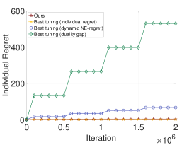
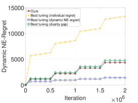
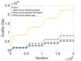
Figure 1: Empirical results of our algorithm (red line) compared with the base-learners with different step size choices. “Best tuning (measure)” represents the curve of the base-learner with the step size choice that performs the best with respect to this “measure” compared with all the other step size configurations. The three figures show that our algorithm’s performance under all of the three measure is comparable to (or even better than) the base-learner with the corresponding best step size tuning. On the other hand, the base-learner specifically tuned for a single measure cannot perform well in all of the three measures simultaneously.

References

- Balasubramanian & Ghadimi (2021) Balasubramanian, K. and Ghadimi, S. Zeroth-order nonconvex stochastic optimization: Handling constraints, high dimensionality, and saddle points. Foundations of Computational Mathematics, pp. 1–42, 2021.
- Besbes et al. (2015) Besbes, O., Gur, Y., and Zeevi, A. J. Non-stationary stochastic optimization. Operations Research, 63(5):1227–1244, 2015.
- Cardoso et al. (2019) Cardoso, A. R., Abernethy, J. D., Wang, H., and Xu, H. Competing against Nash equilibria in adversarially changing zero-sum games. In Proceedings of the 36th International Conference on Machine Learning (ICML), pp. 921–930, 2019.
- Cesa-bianchi et al. (2012) Cesa-bianchi, N., Gaillard, P., Lugosi, G., and Stoltz, G. Mirror descent meets fixed share (and feels no regret). Advances in Neural Information Processing Systems, 25:980–988, 2012.
- Cesa-Bianchi et al. (2012) Cesa-Bianchi, N., Gaillard, P., Lugosi, G., and Stoltz, G. Mirror descent meets fixed share (and feels no regret). In Advances in Neural Information Processing Systems 25 (NIPS), pp. 989–997, 2012.
- Chen & Teboulle (1993) Chen, G. and Teboulle, M. Convergence analysis of a proximal-like minimization algorithm using bregman functions. SIAM Journal on Optimization, 3(3):538–543, 1993.
- Chen et al. (2021) Chen, L., Luo, H., and Wei, C. Impossible tuning made possible: A new expert algorithm and its applications. In Proceedings of the 34th Conference on Learning Theory (COLT), pp. 1216–1259, 2021.
- Chen & Peng (2020) Chen, X. and Peng, B. Hedging in games: Faster convergence of external and swap regrets. In Advances in Neural Information Processing Systems 33 (NeurIPS), pp. 18990–18999, 2020.
- Chiang et al. (2012) Chiang, C.-K., Yang, T., Lee, C.-J., Mahdavi, M., Lu, C.-J., Jin, R., and Zhu, S. Online optimization with gradual variations. In Proceedings of the 25th Conference On Learning Theory (COLT), pp. 6.1–6.20, 2012.
- Daskalakis & Panageas (2019) Daskalakis, C. and Panageas, I. Last-iterate convergence: Zero-sum games and constrained min-max optimization. In Proceedings of the 10th Innovations in Theoretical Computer Science (ITCS) Conference, 2019.
- Daskalakis et al. (2015) Daskalakis, C., Deckelbaum, A., and Kim, A. Near-optimal no-regret algorithms for zero-sum games. Games and Economic Behavior, 92:327–348, 2015.
- Daskalakis et al. (2021) Daskalakis, C., Fishelson, M., and Golowich, N. Near-optimal no-regret learning in general games. In Advances in Neural Information Processing Systems 34 (NeurIPS), pp. to appear, 2021.
- Duvocelle et al. (2021) Duvocelle, B., Mertikopoulos, P., Staudigl, M., and Vermeulen, D. Multi-agent online learning in time-varying games. Mathematics of Operations Research, to appear, 2021.
- Fiez et al. (2021) Fiez, T., Sim, R., Skoulakis, S., Piliouras, G., and Ratliff, L. J. Online learning in periodic zero-sum games. In Advances in Neural Information Processing Systems 34 (NeurIPS), pp. to appear, 2021.
- Freund & Schapire (1999) Freund, Y. and Schapire, R. E. Adaptive game playing using multiplicative weights. Games and Economic Behavior, 29(1-2):79–103, 1999.
- Herbster & Warmuth (1998) Herbster, M. and Warmuth, M. K. Tracking the best expert. Machine learning, 32(2):151–178, 1998.
- Hsieh et al. (2021) Hsieh, Y.-G., Antonakopoulos, K., and Mertikopoulos, P. Adaptive learning in continuous games: Optimal regret bounds and convergence to Nash equilibrium. In Proceedings of the 34th Conference on Learning Theory (COLT), pp. 2388–2422, 2021.
- Luo & Schapire (2015) Luo, H. and Schapire, R. E. Achieving all with no parameters: AdaNormalHedge. In Proceedings of the 28th Annual Conference Computational Learning Theory (COLT), pp. 1286–1304, 2015.
- Pogodin & Lattimore (2019) Pogodin, R. and Lattimore, T. On first-order bounds, variance and gap-dependent bounds for adversarial bandits. In Proceedings of the 35th Conference on Uncertainty in Artificial Intelligence (UAI), pp. 894–904, 2019.
- Rakhlin & Sridharan (2013) Rakhlin, A. and Sridharan, K. Optimization, learning, and games with predictable sequences. In Advances in Neural Information Processing Systems 26 (NIPS), pp. 3066–3074, 2013.
- Roy et al. (2019) Roy, A., Chen, Y., Balasubramanian, K., and Mohapatra, P. Online and bandit algorithms for nonstationary stochastic saddle-point optimization. arXiv preprint arXiv:1912.01698, 2019.
- Syrgkanis et al. (2015) Syrgkanis, V., Agarwal, A., Luo, H., and Schapire, R. E. Fast convergence of regularized learning in games. In Advances in Neural Information Processing Systems 28 (NIPS), pp. 2989–2997, 2015.
- von Neumann (1928) von Neumann, J. Zur theorie der gesellschaftsspiele. Mathematische Annalen, 100:295–320, 1928.
- Wei et al. (2016) Wei, C.-Y., Hong, Y.-T., and Lu, C.-J. Tracking the best expert in non-stationary stochastic environments. In Advances in Neural Information Processing Systems 29 (NIPS), pp. 3972–3980, 2016.
- Wei et al. (2021) Wei, C.-Y., Lee, C.-W., Zhang, M., and Luo, H. Linear last-iterate convergence in constrained saddle-point optimization. In Proceedings of the 9th International Conference on Learning Representations (ICLR), 2021.
- Yang et al. (2016) Yang, T., Zhang, L., Jin, R., and Yi, J. Tracking slowly moving clairvoyant: Optimal dynamic regret of online learning with true and noisy gradient. In Proceedings of the 33rd International Conference on Machine Learning (ICML), pp. 449–457, 2016.
- Zhang et al. (2018) Zhang, L., Lu, S., and Zhou, Z.-H. Adaptive online learning in dynamic environments. In Advances in Neural Information Processing Systems 31 (NeurIPS), pp. 1330–1340, 2018.
- Zhang et al. (2020) Zhang, Y.-J., Zhao, P., and Zhou, Z.-H. A simple online algorithm for competing with dynamic comparators. In Proceedings of the 36th Conference on Uncertainty in Artificial Intelligence (UAI), pp. 390–399, 2020.
- Zhao & Zhang (2021) Zhao, P. and Zhang, L. Improved analysis for dynamic regret of strongly convex and smooth functions. In Proceedings of the 3rd Conference on Learning for Dynamics and Control (L4DC), pp. 48–59, 2021.
- Zhao et al. (2020) Zhao, P., Zhang, Y.-J., Zhang, L., and Zhou, Z.-H. Dynamic regret of convex and smooth functions. In Advances in Neural Information Processing Systems 33 (NeurIPS), pp. 12510–12520, 2020.
- Zhao et al. (2021) Zhao, P., Zhang, Y.-J., Zhang, L., and Zhou, Z.-H. Adaptivity and non-stationarity: Problem-dependent dynamic regret for online convex optimization. ArXiv preprint, arXiv:2112.14368, 2021.
- Zinkevich (2003) Zinkevich, M. Online convex programming and generalized infinitesimal gradient ascent. In Proceedings of the 20th International Conference on Machine Learning (ICML), pp. 928–936, 2003.