Faster Convergence of Local SGD for Over-Parameterized Models

Abstract

Modern machine learning architectures are often highly expressive. They are usually over-parameterized and can interpolate the data by driving the empirical loss close to zero. We analyze the convergence of Local SGD (or FedAvg) for such over-parameterized models in the heterogeneous data setting and improve upon the existing literature by establishing the following convergence rates. We show an error bound of $\mathcal{O}(\exp(-T))$ for strongly-convex loss functions, where $T$ is the total number of iterations. For general convex loss functions, we establish an error bound of $\mathcal{O}(1/T)$ under a mild data similarity assumption and an error bound of $\mathcal{O}(K/T)$ otherwise, where $K$ is the number of local steps. We also extend our results for non-convex loss functions by proving an error bound of $\mathcal{O}(K/T)$. Before our work, the best-known convergence rate for strongly-convex loss functions was $\mathcal{O}(\exp(-T/K))$, and none existed for general convex or non-convex loss functions under the over-parameterized setting. We complete our results by providing problem instances in which such convergence rates are tight to a constant factor under a reasonably small stepsize scheme. Finally, we validate our theoretical results by performing large-scale numerical experiments on both real and synthetic data that reveal the convergence behavior of Local SGD for practical over-parameterized deep learning models.

I Introduction

Distributed optimization methods have become increasingly popular in modern machine learning, owing to the data privacy/ownership issues and the scalability of learning models with respect to massive datasets. The large datasets often make training the model and storing the data in a centralized way almost infeasible. That mandates the use of distributed optimization methods for training machine learning models. However, a critical challenge in distributed optimization is to reduce the communication cost among the local nodes, which has been reported as a major bottleneck in training many large-scale deep learning models [34, 19].

One naive approach to tackling this challenge is using the Minibatch Stochastic Gradient Descent (SGD) algorithm, which generalizes SGD to the distributed optimization setting by averaging the stochastic gradient steps computed at each node (or client) to update the model on the central server. Minibatch SGD has been shown to perform well in a variety of applications, see, e.g., [7, 6]. Recently, Local SGD [26, 21] (also known as Federated Averaging) has attracted significant attention as an appealing alternative to Minibatch SGD to reduce communication cost, where during a communication round, a number of local SGD iterations are performed at each node before the central server computes the average.

Local SGD has been widely applied in Federated Learning [17], and other large-scale optimization problems and has shown outstanding performance in both simulation results [22] as well as real-world applications such as keyboard prediction [10]. At the same time, recent works have studied the theoretical convergence guarantees of Local SGD in various settings [18, 15, 9, 23, 30]. Specifically, an $\mathcal{O}(\frac{1}{nT})$ convergence rate was shown for strongly convex loss functions [13], where $n$ is the number of nodes and $T$ is the total number of iterations. Moreover, an $\mathcal{O}(\frac{1}{\sqrt{nT}})$ convergence rate was shown for general convex loss functions [14]. In addition, an $\mathcal{O}(\frac{1}{\sqrt{nT}})$ convergence rate was shown for non-convex loss functions [31]. These works made substantial progress towards understanding the theoretical convergence properties of the Local SGD. Their results are for general models without the over-parameterization (or interpolation) assumption.

However, despite past efforts, the current results have shortcomings to explain faster convergence of Local SGD compared to Minibatch SGD, which is significant especially when training large-scale deep learning models [22]. In [29], the authors give a lower bound on the performance of local SGD that is worse than the Minibatch SGD guarantee in the i.i.d. data setting (i.e., when all local loss functions are identical). The situation is even worse in the heterogeneous data setting (i.e., when local loss functions are different), which is the setting that we consider in this paper. Local SGD is shown to suffer from “client drift”, resulting in unstable and slow convergence [13], and it is known that Minibatch SGD dominates all existing analyses of Local SGD. [28].

On the other hand, a key observation for explaining the fast convergence of SGD in modern machine learning was made by [20] that says modern machine learning architectures are often highly expressive, and they are over-parameterized. Based on both theoretical and empirical evidence [33, 5], most or all local minima in such over-parametrized settings are also global. Therefore, the authors in [20] assumed interpolation of the data: the empirical loss can be driven close to zero. Under such interpolation assumption, a faster convergence rate of SGD was proven [20, 27]. Furthermore, it was shown that a mini-batch size larger than some threshold $m^{*}$ is essentially helpless for SGD. This is important since, in distributed optimization, it means: for Minibatch SGD, larger batch sizes will not speed up convergence, while for Local SGD, more local steps can potentially speed up convergence. This provides a new direction for explaining the fast convergence of Local SGD for large-scale optimization problems as well as its faster convergence compared to Minibatch SGD.

Motivated by the above studies, in this paper, we formally study the theoretical convergence guarantees of Local SGD for training over-parameterized models in the heterogeneous data setting. Our results improve the existing literature and include the natural case of training large-scale deep learning models.

Our main contributions can be summarized as follows:

• For strongly convex loss functions, an error bound of $\mathcal{O}(\exp(-T))$ can be achieved, where $T$ is the total number of iterations. Before our work, the best-known convergence rate was $\mathcal{O}(\exp(-T/K))$ [24, 15], where $K$ is the total number of local steps.

• For general convex loss functions, we establish an error bound of $\mathcal{O}(1/T)$ under a mild data similarity assumption and an error bound of $\mathcal{O}(K/T)$, otherwise. Before our work, [32] showed the asymptotic convergence of Local Gradient Descent (GD) in this setting but did not provide an explicit convergence rate. To the best of our knowledge, no convergence rate has been established in the past literature under this setting.

• For nonconvex loss functions, we prove an error bound of $\mathcal{O}(K/T)$. To the best of our knowledge, no theoretical analysis of Local SGD in this setting existed in the literature.

• We provide two problem instances to show that our convergence rates for the case of general convex and nonconvex functions are tight up to a constant factor under a reasonably small stepsize scheme.

• We perform large-scale numerical experiments on both real and synthetic data that reveal the convergence behavior of Local SGD for practical over-parameterized deep learning models, hence validating our theoretical results.

In fact, by establishing the above error bounds, we prove the effectiveness of local steps in speeding up the convergence of Local SGD in various settings, thus partially explaining the fast convergence of Local SGD (especially when compared to Minibatch SGD) when training large-scale deep learning models.

In Section II, we formally introduce the problem. In Section III, we state our main convergence results for various types of strongly convex, convex, and non-convex local functions. We also provide a lower bound to show the tightness of our convergence rate bounds for reasonably small step sizes. We justify our theoretical bounds through extensive numerical results in Section IV. Conclusions are given in Section V. We defer all the proofs to Section VI.

II Problem Formulation

We consider the problem of $n$ nodes $[n]=\{1,2,\ldots,n\}$ that collaboratively want to learn an over-parameterized model with decentralized data as the following distributed stochastic optimization problem:

$$\min_{\mathbf{x}\in\mathbb{R}^{d}}\ f(\mathbf{x}):=\frac{1}{n}\sum_{i=1}^{n}f_{i}(\mathbf{x}),\$$ (1)

where the function $f_{i}(\mathbf{x})\triangleq\mathbb{E}_{\xi_{i}\sim\mathcal{D}_{i}}f_{i}(\mathbf{x},\xi_{i})$ denotes the local loss function, $\xi_{i}$ is a stochastic sample that node $i$ has access to, and $\mathcal{D}_{i}$ denotes the local data distribution over the sample space $\Omega_{i}$ of node $i$.

We assume $f(\mathbf{x})$ is bounded below by $f^{\star}$ (i.e., a global minimum exists), $f_{i}(\mathbf{x},\xi_{i})$ is $L$-smooth for every $i\in[n]$, and $\nabla f_{i}(\mathbf{x},\xi_{i})$ is an unbiased stochastic gradient of $f_{i}(\mathbf{x})$. Moreover, for some of our results, we will require functions $f_{i}(\mathbf{x},\xi_{i})$ to be $\mu$-strongly convex with respect to the parameter $\mathbf{x}$ as defined next.

Assumption 1 ($\mu$-strong convexity).

There exists a constant $\mu\geq 0$, such that for any $\mathbf{x},\mathbf{y}\in\mathbb{R}^{d},i\in[n]$, and $\xi_{i}\in\Omega_{i}$, we have

$$f_{i}(\mathbf{x},\xi_{i})\geq f_{i}(\mathbf{y},\xi_{i})+\langle\nabla f_{i}(\mathbf{y},\xi_{i}),\mathbf{x}-\mathbf{y}\rangle+\frac{\mu}{2}\|\mathbf{x}-\mathbf{y}\|^{2}.$$ (2)

If $\mu=0$, we simply say that each $f_{i}$ is convex.

The over-parameterized setting, i.e., when the model can interpolate the data completely such that the loss at every data point is minimized simultaneously (usually means zero empirical loss), can be characterized by the following two assumptions [20, 27]:

Assumption 2 (Interpolation).

Let $\mathbf{x}^{\star}\in\operatorname*{arg\,min}_{x\in\mathbb{R}^{d}}f(\mathbf{x})$. Then, $\nabla f_{i}(\mathbf{x}^{\star},\xi_{i})=0,\ \forall i\in[n],\ \xi_{i}\in\Omega_{i}$.

Assumption 3 (Strong Growth Condition (SGC)).

There exists constant $\rho$ such that $\forall\mathbf{x}\in\mathbb{R}^{d},\ i\in[n]$,

$$\mathbb{E}_{\xi_{i}\sim\mathcal{D}_{i}}\|\nabla f_{i}(\mathbf{x},\xi_{i})\|^{2}\leq\rho\|\nabla f(\mathbf{x})\|^{2}.$$ (3)

Notice that for the functions to satisfy SGC, local gradients at every data point must all be zero at the optimum $x^{\star}$. Thus, SGC is a stronger assumption than interpolation, which means Assumption 3 implies Assumption 2.

Assumption 2 is commonly satisfied by modern machine learning model such as deep neural networks [25] and kernel machines [3]. [27] discussed functions satisfying Assumption 3 and showed that under additional assumptions on the data, the squared-hinge loss satisfies the assumption.

When the local loss functions are convex, we define the following quantity $c\in[0,1]$ that allows us to measure the dissimilarity among them.

Definition 1.

Let Assumptions 1 and 2 hold with $\mu\geq 0$. Let ${\mathbf{x}}^{*}\in\operatorname*{arg\,min}_{x\in\mathbb{R}^{d}}f({\mathbf{x}})$. We define $c$ as the largest real number such that for all ${\mathbf{x}}_{1},\ldots{\mathbf{x}}_{n}\in\mathbb{R}^{d}$ and $\bar{\mathbf{x}}\coloneqq\frac{1}{n}\sum_{i=1}^{n}{\mathbf{x}}_{i}$, we have

$$\frac{1}{n}\sum_{i=1}^{n}(f_{i}({\mathbf{x}}_{i})-f_{i}({\mathbf{x}}^{*}))\geq c(f(\bar{\mathbf{x}})-f({\mathbf{x}}^{*})).$$ (4)

If Assumptions 1 and 2 hold, the left hand side of (4) is always non-negative, which implies $c\geq 0$. In particular, by taking ${\mathbf{x}}_{1}=\ldots={\mathbf{x}}_{n}$ we have $c\leq 1$. Moreover, as the local loss functions become more similar, $c$ will become closer to $1$. In particular, in the case of homogeneous local loss functions, i.e., $f_{i}=f\ \forall i$, using Jensen’s inequality we have $c=1$.

In the next section, we will proceed to establish our main convergence rate results for various settings of strongly convex, convex, and nonconvex local functions.

III Convergence of Local SGD

This section reviews Local SGD and then analyzes its convergence rate under the over-parameterized setting.

In Local SGD, each node performs local gradient steps, and after every $K$ steps, sends the latest model to the central server. The server then computes the average of all nodes’ parameters and broadcasts the averaged model to all nodes. Let $T$ be the total number of iterations in the algorithm. There is a set of communication times ${\mathcal{I}}=\{0,K,2K,\ldots,T=RK\}$, and in every iteration $t$, Local SGD does the following: i) each node performs stochastic gradient updates locally based on $\nabla f_{i}(\mathbf{x},\xi_{i})$, which is an unbiased estimation of $\nabla f_{i}(\mathbf{x})$, and ii) if $t$ is a communication time, i.e., $t\in{\mathcal{I}}$, it sends the current model to the central server and receives the average of all nodes’ models. The pseudo-code for the Local SGD algorithm is provided in Algorithm 1.

Algorithm 1 Local SGD

1:  Input: ${\mathbf{x}}_{i}^{(0)}={\mathbf{x}}^{(0)}$ for $i\in[n]$, number of iterations $T$, the stepsize $\eta$, the set of communication times ${\mathcal{I}}$.

2:  for $t=0,\ldots,T-1$ do

3:     for $i=1,\ldots,n$ do

4:        Sample $\xi_{i}^{(t)}$, compute $\nabla f_{j}(\mathbf{x}_{i}^{(t)}\!,\xi_{i}^{(t)})$

5:        $\mathbf{x}_{i}^{(t+\frac{1}{2})}=\mathbf{x}_{i}^{(t)}-\eta\nabla f_{i}(\mathbf{x}_{i}^{(t)}\!,\xi_{i}^{(t)})$

6:        if $t+1\in{\mathcal{I}}$ then

7:           $\mathbf{x}_{i}^{(t+1)}=\frac{1}{n}\sum_{j=1}^{n}\mathbf{x}_{i}^{(t+\frac{1}{2})}$

8:        else

9:           $\mathbf{x}_{i}^{(t+1)}=\mathbf{x}_{i}^{(t+\frac{1}{2})}$

10:        end if

11:     end for

12:  end for

III-A Convergence Rate Analysis

We now state our main result on the convergence rate of Local SGD under over-parameterized settings for strongly convex functions.

Theorem 1 (Strongly convex functions).

Let Assumptions 1,2 hold with $\mu>0$. If we follow algorithm 1 with stepsize $\eta={1}/{L}$, we will have

$$\mathbb{E}\|\bar{\mathbf{x}}^{(T)}-{\mathbf{x}}^{*}\|^{2}\leq\big{(}1-\frac{\mu}{L}\big{)}^{T}\|{\mathbf{x}}^{(0)}-{\mathbf{x}}^{*}\|^{2},$$ (5)

where $\bar{\mathbf{x}}^{(t)}\coloneqq\frac{1}{n}\sum_{i=1}^{n}{\mathbf{x}}_{i}^{(t)}$ is the average of all nodes’ iterates at time step $t$.

It was shown in [24, 15] that Local SGD achieves a geometric convergence rate for strongly convex loss functions in the over-parameterized setting. However, both [24] and [15] give an $\mathcal{O}(\exp(-{T}/{K}))$ convergence rate, while our convergence rate is $\mathcal{O}(\exp(-T))$. The difference between these two rates is significant because the former rate implies that local steps do not contribute to the error bound (since the convergence rate essentially depends on the number of communication rounds $R={T}/{K}$). In contrast, the latter rate suggests local steps can drive the iterates to the optimal solution exponentially fast. The difference between the rates in [24, 15] and Theorem 1 can be explained by the fact that [24, 15] use a smaller stepsize of $\eta=\mathcal{O}(\frac{1}{KL})$, while our analysis allows a larger stepsize of $\eta={1}/{L}$. On the other hand, we note that the $\mathcal{O}(\exp(-T))$ convergence rate given in Theorem 1 for Local SGD can be the best one can hope for, since in general, one should not expect $\bar{\mathbf{x}}$ to converge faster than the fastest converging local ${\mathbf{x}}_{i}$ to the optimal point, where the latter has a convergence rate of $\mathcal{O}(\exp(-T))$. Therefore, further improvement in the convergence rate may require a different learning scheme than Local SGD.

The next theorem states the convergence rates for general convex loss functions:

Theorem 2 (General convex functions).

Let Assumptions 1, 2 hold with $\mu=0$, let $c$ be defined as in Definition 1. Moreover, let

$$w_{t}=\begin{cases}1&\ \mbox{if}\ t\in{\mathcal{I}}\ \mbox{or}\ t+1\in{\mathcal{I}},\\ c&\mbox{otherwise},\end{cases}$$

and define $W=\sum_{t=0}^{T-1}w_{t}$ and $\hat{{\mathbf{x}}}^{T}\triangleq\frac{1}{W}\sum_{i=0}^{T-1}w_{t}\bar{\mathbf{x}}^{(t)}$. If we follow Algorithm 1 with stepsize $\eta=\frac{1}{2L}$ and $K\geq 2$, then we have

$$\mathbb{E}[f(\hat{{\mathbf{x}}}^{T})-f^{*}]\leq\frac{2KL\|{\mathbf{x}}^{(0)}-{\mathbf{x}}^{*}\|^{2}}{cKT+2(1-c)T}.$$ (6)

The convergence of Local GD for general convex loss functions in the over-parameterized setting was shown earlier in [32] without giving an explicit convergence rate. Instead, for similarity parameters $c>0$ and $c=0$, we give convergence rates of $\mathcal{O}({1}/{T})$ and $\mathcal{O}({K}/{T})$ for Local SGD, respectively. The significant difference between the convergence rates for the case of $c>0$ and $c=0$ suggests that having slight similarity in the local loss functions is critical to the performance of Local SGD, which also complies with the simulation findings in  [22]. To the best of our knowledge, Theorem 2 provides the first $\mathcal{O}({1}/{T})$ or $\mathcal{O}({K}/{T})$ convergence rates for Local SGD for general convex loss functions in the over-parameterized setting. On the other hand, in Section III-B, we provide a problem instance suggesting that in the worst case, the $\mathcal{O}({K}/{T})$ convergence rate obtained here might be tight up to a constant factor.

It is worth noting that the speedup effect of local steps when $c>0$ is a direct consequence of the $\mathcal{O}({1}/{T})$ convergence rate shown in Theorem 2. When $c=0$, a closer look at (6) and the weights $w_{t}$ reveals that $w_{t}=1$ if $t\in{\mathcal{I}}$ or $t+1\in{\mathcal{I}}$, implying that at least the first or the last local steps during each communication round is “effective”. This, in turn, shows that local steps can speed up the convergence of Local SGD by at least a factor of $2$.

Finally, for the case of non-convex loss functions, we have the following result.

Theorem 3 (Non-convex functions).

Let Assumption 3 hold. If we follow Algorithm 1 with stepsize $\eta=\frac{1}{3KL\rho}$, and $K\geq 2$, we will have

$$\min_{0\leq t\leq T-1}\mathbb{E}\|\nabla f(\bar{\mathbf{x}}^{t})\|^{2}\leq\frac{27KL\rho(f({\mathbf{x}}_{0})-f^{*})}{T}.$$ (7)

Theorem provides an $\mathcal{O}({K}/{T})$ convergence rate for Local SGD for non-convex loss functions in the over-parameterized setting, which is the first $\mathcal{O}({1}/{T})$ convergence rate for Local SGD under this setting. However, this rate is somewhat disappointing as it suggests that local steps may not help the algorithm to converge faster. This is mainly caused by the choice of stepsize $\eta=\frac{1}{3KL\rho}$, which is proportional to ${1}/{K}$. On the other hand, in Section III-B, we argue that this choice of stepsize may be inevitable in the worst case because there are instances for which the choice of stepsize $\eta$ greater than $\mathcal{O}({1}/{K})$ results in divergence of the algorithm.

III-B Lower Bounds for Local SGD with Stepsize $\eta\leq\frac{1}{L}$

In this section, we present two instances of Problem (1) showing that the convergence rates shown in Section III-A are indeed tight up to a constant factor, provided that Algorithm 1 is run with reasonably small stepsize $\eta$. Specifically, we show that if Local SGD is run with stepsize $\eta\leq\frac{1}{L},$ then:

1. for general convex loss functions, there exist functions $f_{i}$ satisfying Assumptions 1 and 2 with $\mu=0$ and $c=0$, such that Local SGD incurs an error bound of $f(\bar{\mathbf{x}}^{T})-f^{*}=\Omega({KL}/{T})$.

2. for non-convex loss functions, there exist functions $f_{i}$ satisfying Assumption 3, such that Local SGD with a stepsize $\eta\geq\frac{2}{LK}$ will not converge to a first-order stationary point.

Proposition 1 (General Convex Functions).

There exists an instance of general convex loss functions $f_{i}$ satisfying Assumptions 1 and 2 with $\mu=0$ and $c=0$, such that Local SGD incurs an error bound of $f(\bar{\mathbf{x}}^{T})-f^{*}=\Omega({KL}/{T})$.

Proof.

Consider Problem (1) in the following setting. Let $n=4R={4T}/{K},\ d=1$, and $f_{1}(x)=\frac{L}{2}x^{2},\ f_{2}(x)=f_{3}(x)=\cdots=f_{n}(x)=0$. Then $f(x)=\frac{L}{2n}x^{2}$, and clearly every $f_{i}$ is $L$-smooth and satisfies Assumptions 1 and 2 with $\mu=0,\ c=0$. Suppose Algorithm 1 is run with stepsize $\eta\leq\frac{1}{L}$, and initialized at ${\mathbf{x}}^{0}=1$. We will show that $\min_{t\in[T]}(f(\bar{\mathbf{x}}^{t})-f^{*})\geq\frac{KL}{16T}$. To that end, first we note that the global optimal point is ${\mathbf{x}}^{*}=0$, and local gradient steps for all nodes except node $1$ keeps local variable unchanged. Moreover, since $\eta\leq{1}/{L}$, we have ${\mathbf{x}}_{1}^{t}\in[0,1],\ \forall t\in[T]$. Therefore, $\{\bar{\mathbf{x}}^{t}\}$ is a non-increasing sequence that lies in interval $[0,1]$. Thus, we only need to show $f(\bar{\mathbf{x}}^{T})\geq\frac{KL}{16T}.$

Next, we claim that $\bar{\mathbf{x}}^{(r+1)K}\geq\frac{n-1}{n}\bar{\mathbf{x}}^{rK},\ \forall r$. In fact, since ${\mathbf{x}}_{1}^{(r+1)K-1/2}\geq 0$ and ${\mathbf{x}}_{i}^{(r+1)K-1/2}=\bar{\mathbf{x}}^{rK}$, for $i=2,\ldots,n$, we have

$$\bar{\mathbf{x}}^{(r+1)K}=\frac{1}{n}\sum_{i=1}^{n}{\mathbf{x}}_{i}^{(r+1)K-1/2}\geq\frac{n-1}{n}\bar{\mathbf{x}}^{rK}.$$

Therefore, we can write

$$f(\bar{\mathbf{x}}^{T}) =\frac{L}{2n}(\bar{\mathbf{x}}^{T})^{2}\geq\frac{L}{2n}(\frac{n-1}{n})^{2R}$$

$$\geq\frac{L}{2n}(1-\frac{2R}{n})=\frac{L}{16R}=\frac{KL}{16T},$$

which completes the proof. ∎

Proposition 2 (Non-convex Functions).

There exists an instance of nonconvex loss functions $f_{i}$ satisfying Assumption 3, such that Local SGD with a stepsize $\eta\geq\frac{2}{LK}$ will not converge to a first-order stationary point.

Proof.

Consider Problem (1) in the following setting. Let $n=2$, $d=1$ and $f_{1}(x)=\frac{L}{2}x^{2},f_{2}(x)=-\frac{L}{4}x^{2}$. Then $f(x)=\frac{L}{4}x^{2}$, and clearly every $f_{i}$ is $L$-smooth and satisfies Assumptions 3 with $\rho=2$. Suppose Algorithm 1 is run with stepsize $\eta\leq{1}/{L}$ and initialized at ${\mathbf{x}}^{0}=1$. We want to show that for such distributed stochastic optimization problem, if we run Algorithm 1 for any stepsize $\eta\geq\frac{2}{LK}$, the gradient norm at any iterate will be lower bounded by $\min_{t\in[T]}\|\nabla f(\bar{\mathbf{x}}^{t})\|^{2}\geq\frac{L^{2}}{16}$.

First, we note that the global optimal point is ${\mathbf{x}}^{*}=0$, which is the only critical point. Since $\eta\leq{1}/{L}$, we have ${\mathbf{x}}_{1}^{t}\geq 0,\ \forall t\in[T]$, and local gradient steps for node $2$ will always increase the value of ${\mathbf{x}}_{2}^{t}$. Next, we claim that if $\eta\geq\frac{2}{LK}$, then $\bar{\mathbf{x}}^{rK}\geq 1,\ \forall r$, and prove it by induction. First notice that $\bar{\mathbf{x}}^{0}=1\geq 1$. Suppose $\bar{\mathbf{x}}^{rK}\geq 1$, then

$${\mathbf{x}}_{2}^{(r+1)K-\frac{1}{2}} =\bar{\mathbf{x}}^{rK}-\eta\sum_{t=rK}^{(r+1)K-1}\nabla f_{2}({\mathbf{x}}_{2}^{t})$$

$$=\bar{\mathbf{x}}^{rK}+\eta\sum_{t=rK}^{(r+1)K-1}\frac{L}{2}{\mathbf{x}}_{2}^{t}$$

$$\geq 1+\frac{2}{LK}\sum_{t=rK}^{(r+1)K-1}\frac{L}{2}=2.$$

Since ${\mathbf{x}}_{1}^{(r+1)K-1/2}\geq 0$, we have

$$\bar{\mathbf{x}}^{(r+1)K}=\frac{1}{2}({\mathbf{x}}_{1}^{(r+1)K-1/2}+{\mathbf{x}}_{2}^{(r+1)K-1/2})\geq 1,$$

which proves the claim. Therefore, ${\mathbf{x}}_{2}^{t}\geq 1,\ \forall t\in[T]$ and ${\mathbf{x}}_{1}^{t}\geq 0,\ \forall t\in[T]$, which implies $\bar{\mathbf{x}}^{t}\geq{1}/{2},\forall t\in[T]$. This shows that $\|\nabla f(\bar{\mathbf{x}}^{t})\|^{2}\geq{L^{2}}/{16}$, as desired. ∎

Remark 1.

According to Proposition 2, in the worst case a stepsize of $\eta\leq\mathcal{O}({1}/{K})$ for Local SGD is inevitable. This in view of [27] implies a convergence rate of at most $\mathcal{O}({K}/{T})$.

IV Numerical Analysis

This section shows the results for two sets of experiments on synthetic and real datasets to validate our theoretical findings. For the first set of experiments, we focus on convex and strongly-convex loss functions, where we train a perceptron classifier on a synthetic linearly separable dataset. For the second set of experiments, we focus on non-convex loss functions, where we train an over-parameterized ResNet18 neural network [11] on the Cifar10 dataset [16].

IV-A Perceptron for Linearly Separable Dataset

We generate a synthetic binary classification dataset with $N=10000$ data-points uniformly distributed in a $d=100$ dimensional cube $[-1,1]^{d}$. Then, a hyperplane is randomly generated, and all data points above it are labeled ‘$1$’ with other data points labeled ‘$-1$’, thus ensuring the dataset is linearly separable and satisfies the interpolation property. We divide the dataset among $n=16$ nodes and apply Local SGD to distributedly train a perceptron to minimize the finite-sum squared-hinge loss function:

$$f(w)=\frac{1}{N}\sum_{i=1}^{N}\max(0,1-y_{i}x_{i}^{T}w)^{2}.$$

We partition the dataset in three different ways to reflect different data similarity regimes and evaluate the relationship between training loss, communication rounds, and local steps for Local SGD under each of the three regimes.

• Even partition: The dataset is partitioned evenly to all nodes, resulting in i.i.d. local data distribution. The simulation results for this regime are shown in Figure 1(a).

• Pathological partition: The dataset is partitioned by $17$ hyperplanes that are parallel to the initial hyperplane. Distances between adjacent hyperplanes are the same. Each node gets assigned one of the $16$ ’slices’ of data points. This is a highly heterogeneous data partition since $15$ out of the $16$ nodes will have only one label. The simulation results for this regime are shown in Figure 1(b).

• Worst case partition: All data points are assigned to one node. The other $15$ nodes have an empty dataset. This partition corresponds to the setting in Example 1. The simulation results for this regime are shown in Figure 1(c).

An $\mathcal{O}({1}/T$) Convergence Rate: In general, we can observe a linear speedup of the convergence rate with the number of local steps in all three regimes, implying the $\mathcal{O}(\frac{1}{KR})=\mathcal{O}({1}/{T})$ convergence rate for Local SGD, validating our result in Theorem 2. The simulation results suggest that despite the $\mathcal{O}({K}/{T})$ worst-case upper bound, the optimistic $\mathcal{O}({1}/{T})$ convergence rate in Theorem 2, as well as the effectiveness of local steps, can generally be expected in practice. Finally, we note that the simulation results (especially in Figure 1(c)) do not invalidate our result in Proposition 1, because in Proposition 1, i) all but one node has an empty dataset, and ii) the number of nodes $n$ is proportional to the number of communication rounds $R$. However, these two conditions are rarely satisfied in practice.

Effect of Data Heterogeneity: While in general Local SGD enjoys an $\mathcal{O}(\frac{1}{KR})=\mathcal{O}({1}/{T})$ convergence rate, data heterogeneity is still a key issue and will cause the algorithm to become slower and unstable. Comparing Figure 1(a) with Figure 1(b), we can see that the pathological partition makes the algorithm converge two/three times slower. Moreover, comparing Figure 1(b) with Figure 1(c), we can see that in the worst-case partition regime, the algorithm converges about ten times slower than even the pathological partition regime.

To evaluate the performance of Local SGD for the over-parameterized model with strongly-convex loss functions, we add a correction term to the squared-hinge loss to make it strongly convex and run another experiment on the pathologically partitioned dataset. The result is shown in Figure 2. The $\mathcal{O}(\exp(-KR))=\mathcal{O}(\exp(-T))$ convergence rate can be observed from the figure, validating our result in Theorem 1.

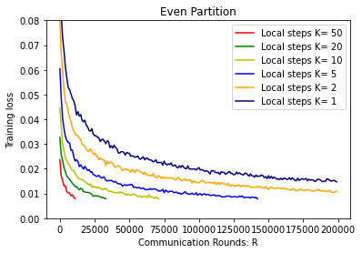
(a)

(b)

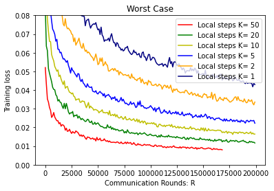
(c)

Figure 1: Training loss vs. communication rounds with different local steps under the three data partition regimes. 1(a): even partition regime. 1(b): pathological partition regime. 1(c): worst case partition regime.

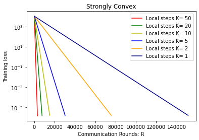
Figure 2: Local SGD for the over-parameterized model with strongly-convex loss functions. Training loss vs. communication rounds with different local steps under the pathological data partition regimes. Training loss is in log scale.

IV-B ResNet18 Neural Network for Cifar10

We distribute the Cifar10 dataset [16] to $n=20$ nodes and apply Local SGD to train a ResNet18 neural network [11]. The neural network has 11 million trainable parameters and, after sufficient training rounds, can achieve close to $0$ training loss, thus satisfying the interpolation property.

For this set of experiments, we run the Local SGD algorithm for $R=20000$ communication rounds with a different number of local steps per communication round $K=1,2,5,10,20$ and report the training error of the global model along the process. We do not report the test accuracy of the model, which is related to the generalization of the model and is beyond the scope of this work. Following the work  [12], we also use Layer Normalization [2] instead of Batch Normalization in the architecture of ResNet18 while keeping everything else the same.

We first sort the data by their label, then divide the dataset into $20$ shards and assign each of $20$ agents $1$ shard. In this way, ten nodes will have image examples of one label, and ten nodes will have image examples of two labels. This regime leads to highly heterogeneous datasets among nodes. We use a training batch size of $8$ and choose stepsize $\eta$ based on a grid search of resolution $10^{-2}$. The simulation results are averaged over $3$ independent runs of the experiments. We show the global landscape of the result in figures 3(a) and 3(b), where the training loss and the reciprocal of the training loss over the communication rounds are reported, respectively. The decrease in the training loss can be divided into Phase 1, Phase 2, and a transition phase between them, as shown in figures 5(a), 5(b), and 5(c).

Phase 1: As figure 5(a) shows, in the first $\approx 3000$ communication rounds, the reciprocal of the training loss grows nearly linearly with respect to the number of communication rounds. This is strong evidence of the $\mathcal{O}({1}/{R})=\mathcal{O}({K}/{T})$ convergence rate of Local SGD as we stated in Theorem 3. We can also see that in this phase, the decrease of training loss depends only on the number of communication rounds $R$ regardless of the number of local steps $K$, thus validating Theorem 3.

Phase 2: After $\approx 6000$ communication rounds, as the training loss further decreases (below 0.01), we can observe from figures 5(c) and figure 4 a clear linear dependence of the reciprocal of the training loss and the total iterations $T$ (notice in figure 4 all lines share similar slope). This corresponds to a $\mathcal{O}({1}/{T})$ convergence rate of Local SGD. In fact, we conjecture that in this phase, the model has moved close enough to the neighborhood of a global optimal point, which simultaneously minimizes the loss at every single data point. Therefore, every local step moves the model closer to that global optimal point regardless of at which node it is performed, causing the aggregation step to be no longer meaningful and resulting in the convergence rate of $\mathcal{O}({1}/{T})$ instead of $\mathcal{O}({1}/{R})$.

To conclude, we have performed large scale experiments that reveal the convergence behavior of Local SGD for practical over-parameterized deep learning models. We observe from the experiments that the decrease of the training loss can be divided into Phase 1, Phase 2, and a transition phase between them. The convergence rate of Local SGD in practice can be $\mathcal{O}({K}/{T})$ (Phase 1), or $\mathcal{O}({1}/{T})$ (Phase 2), or somewhere in between (transition phase). Experimental results in Phase 1 strongly support our theoretical findings in Theorem 3, while experimental results in Phase 2 partially support it and also raise new interesting questions.

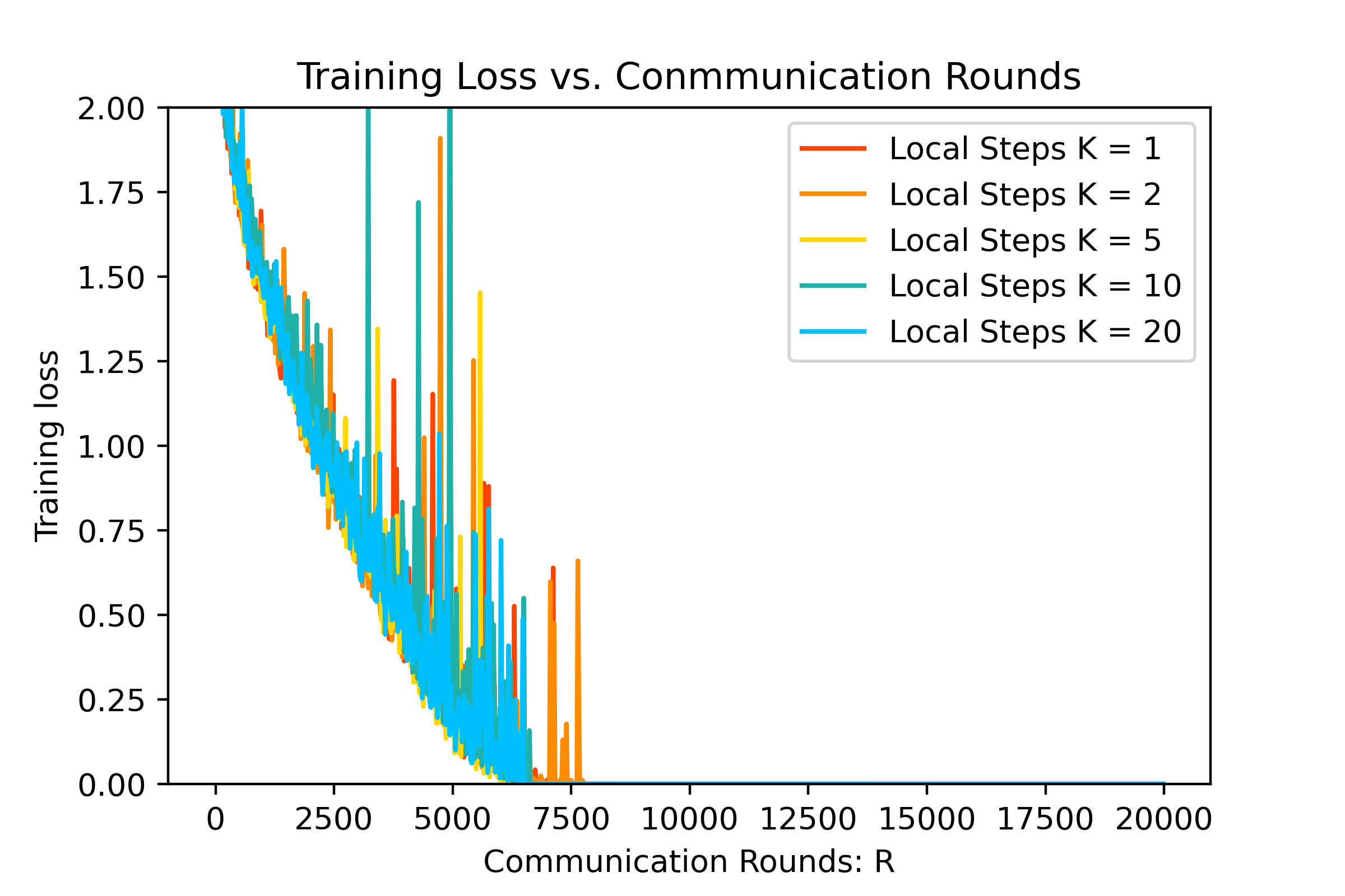
(a)

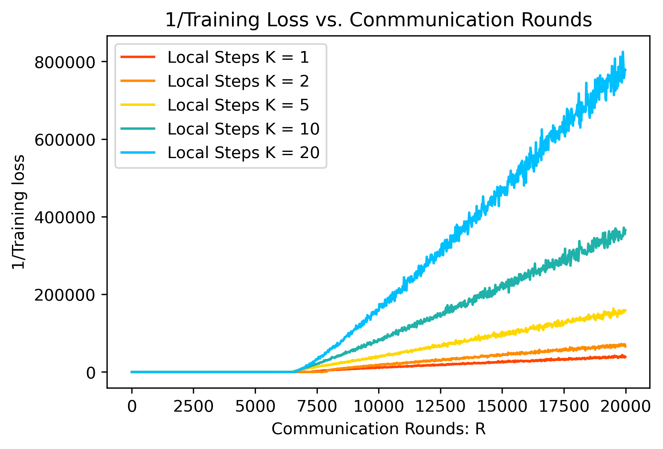
(b)

Figure 3: 3(a): Training loss vs. communication rounds with different local steps. 3(b): 1/Training loss vs. communication rounds with different local steps.

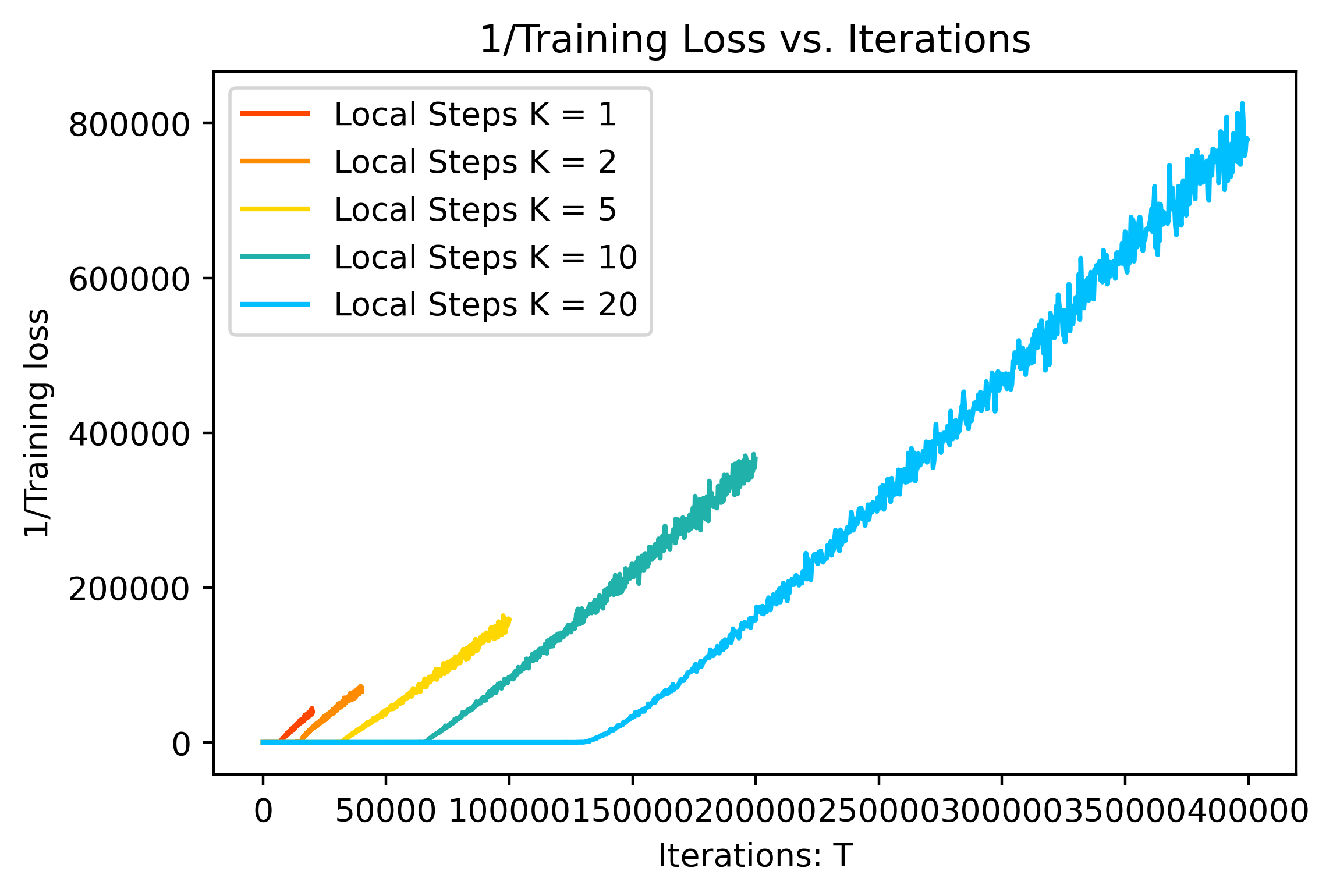
Figure 4: 1/(Training loss) vs. Total number of iterations $T$ with different local steps.

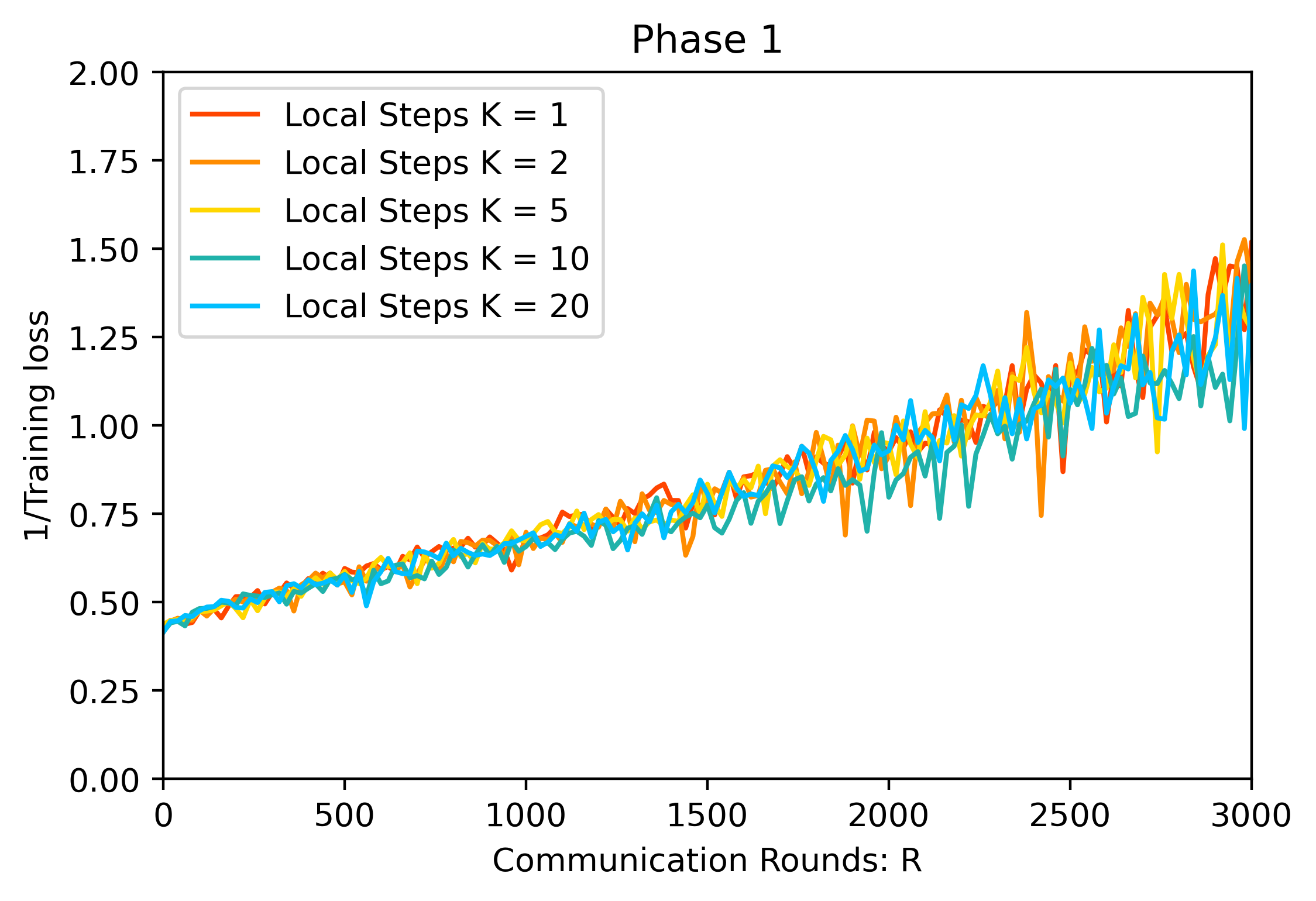
(a)

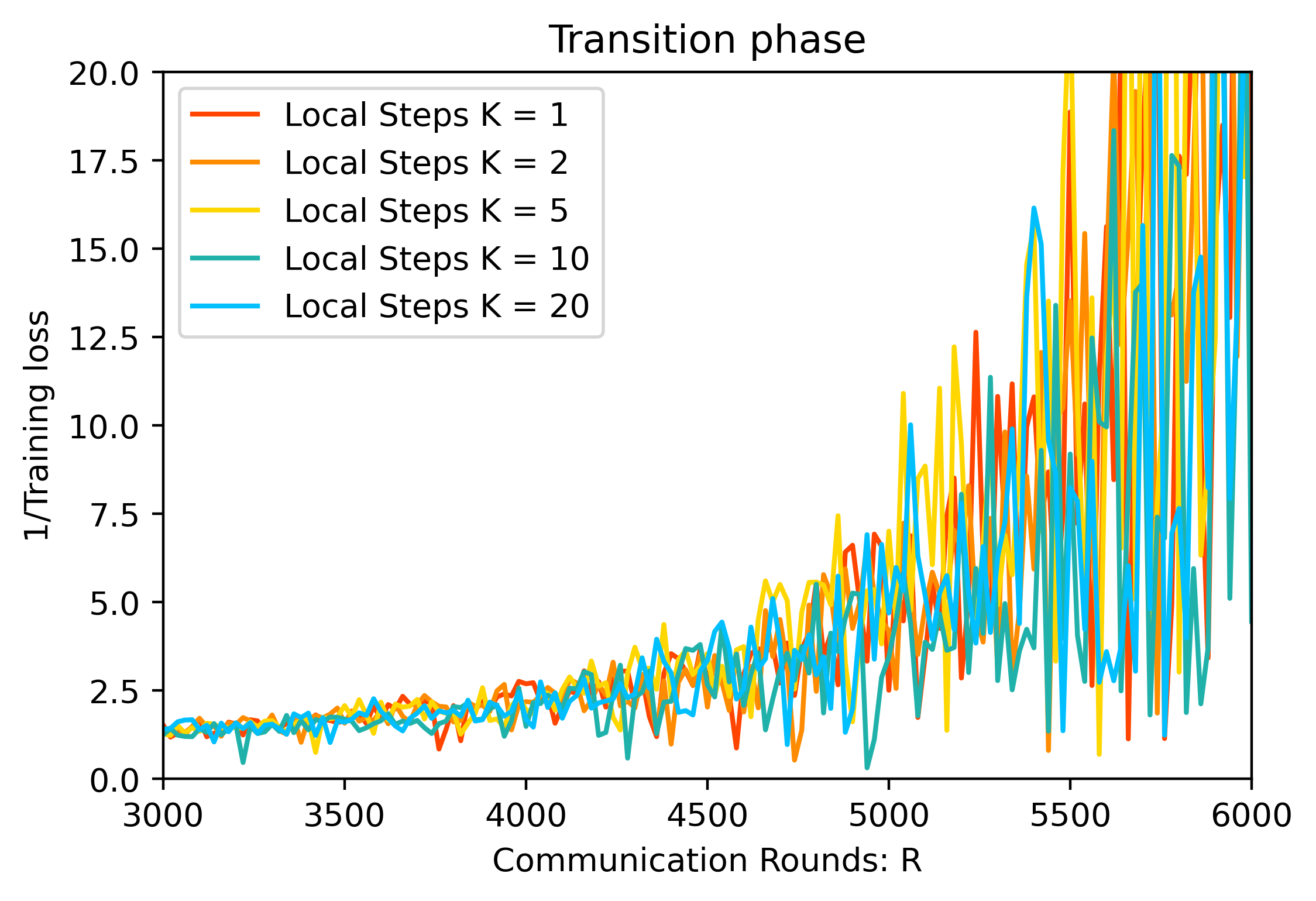
(b)

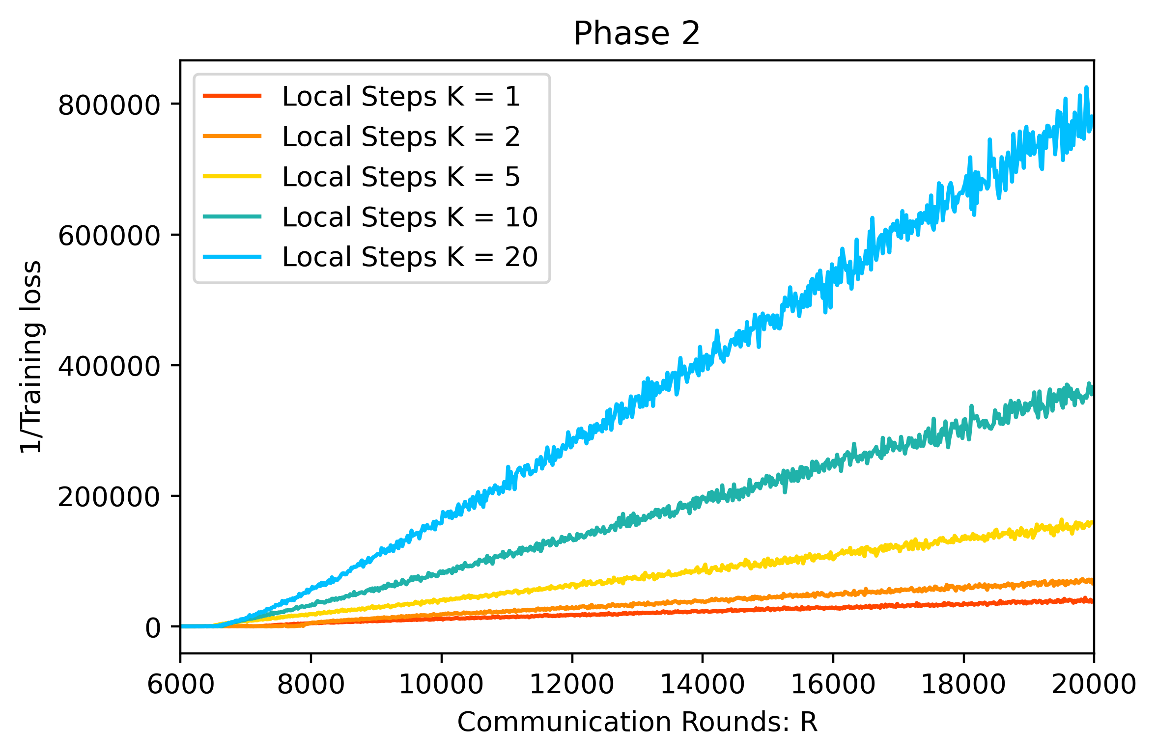
(c)

Figure 5: 1/(Training loss) vs. communication rounds for different phases. 5(a): Phase 1. 1(b): Transition phase. 1(c): Phase 2.

V Conclusion

We studied the theoretical convergence guarantees of Local SGD for training over-parameterized models in the heterogeneous data setting and established tight convergence rates for strongly-convex, convex and non-convex loss functions. Moreover, we validated the effectiveness of local steps in speeding up the convergence of Local SGD in various settings both theoretically and using extensive simulations. Our results partially explain the fast convergence of Local SGD (especially when compared to Minibatch SGD) when training large-scale deep learning models.

As future work, one interesting direction would be to generalize our results to the partial node participation setting, which is practical in federated learning. Another interesting direction would be to further study and quantify the two-phase convergence phenomenon of Local SGD when training large-scale neural networks, as we discussed in Section IV-B. This may need combining the interpolation assumption with the special architectures of neural networks (see, e.g., [1, 8]).

VI Proof of Theorems

Define $\bar{\mathbf{g}}^{(t)}\coloneqq\frac{1}{n}\sum_{i=1}^{n}\nabla f_{i}({\mathbf{x}}_{i}^{(t)},\xi_{i}^{(t)})$ as the average of the stochastic gradients evaluated at all nodes, and $r_{t}\coloneqq\mathbb{E}\|\bar{\mathbf{x}}^{(t)}-{\mathbf{x}}^{*}\|^{2}$ as the expected distance to the optimum solution.

VI-A Preliminary Propositions

Proposition 3.

Let $f:\mathbb{R}^{d}\rightarrow\mathbb{R}$ be an $L$-smooth function and ${\mathbf{x}}^{*}\in\operatorname*{arg\,min}_{x\in\mathbb{R}^{d}}f(\mathbf{x})$. Then,

$$\frac{1}{2L}\|\nabla f({\mathbf{x}})\|^{2}\leq f({\mathbf{x}})-f({\mathbf{x}}^{*})$$ (8)

Proposition 4.

Let $\bar{\mathbf{x}}=\frac{1}{n}\sum_{i=1}^{n}{\mathbf{x}}_{i}$. For any ${\mathbf{x}}^{\prime}\in\mathbb{R}^{d}$, we have

$$\sum_{i=1}^{n}\|{\mathbf{x}}_{i}-{\mathbf{x}}^{\prime}\|^{2}=\sum_{i=1}^{n}\|{\mathbf{x}}_{i}-\bar{\mathbf{x}}\|^{2}+n\|\bar{\mathbf{x}}-{\mathbf{x}}^{\prime}\|^{2}.$$ (9)

As a consequence, we have the following inequalities:

$$\sum_{i=1}^{n}\|{\mathbf{x}}_{i}-\bar{\mathbf{x}}\|^{2}\leq\sum_{i=1}^{n}\|{\mathbf{x}}_{i}\|^{2},$$ (10)

$$\|\bar{\mathbf{x}}-{\mathbf{x}}^{\prime}\|^{2}\leq\frac{1}{n}\sum_{i=1}^{n}\|{\mathbf{x}}_{i}-{\mathbf{x}}^{\prime}\|^{2}.$$ (11)

VI-B Proof of Theorem 1

Let ${\mathbf{x}}^{*}\in\operatorname*{arg\,min}_{x\in\mathbb{R}^{d}}f({\mathbf{x}})$. From Assumptions 2 and 1, we have $\nabla f_{i}(\mathbf{x}^{\star},\xi_{i})=0$, which implies ${\mathbf{x}}^{*}\in\operatorname*{arg\,min}_{x\in\mathbb{R}^{d}}f_{i}({\mathbf{x}},\xi_{i}),\ \forall i\in[n],\ \xi_{i}\in\Omega_{i}$.

We first bound the progress made by local variables ${\mathbf{x}}_{i}$ in one local SGD update as follows:

Lemma 2.

Let Assumptions 1 and 2 hold with $\mu>0$. If we follow Algorithm 1 with stepsize $\eta_{t}=\frac{1}{L}$, we will have

$$\mathbb{E}_{\xi_{i}^{t}}\|{\mathbf{x}}_{i}^{t+\frac{1}{2}}-{\mathbf{x}}^{*}\|^{2}\leq(1-\frac{\mu}{L})\|{\mathbf{x}}_{i}^{t}-{\mathbf{x}}^{*}\|^{2}$$ (12)

Proof.

$$\ \quad\mathbb{E}_{\xi_{i}^{t}}\|{\mathbf{x}}_{i}^{t+\frac{1}{2}}-{\mathbf{x}}^{*}\|^{2}$$

$$=\mathbb{E}_{\xi_{i}^{t}}\|{\mathbf{x}}_{i}^{t}-{\mathbf{x}}^{*}-\eta\nabla f_{i}({\mathbf{x}}_{i}^{t},\xi_{i}^{t})\|^{2}$$

$$=\|{\mathbf{x}}_{i}^{t}\!-\!{\mathbf{x}}^{*}\|^{2}-2\eta\langle{\mathbf{x}}_{i}^{t}\!-\!{\mathbf{x}}^{*},\nabla f_{i}({\mathbf{x}}_{i}^{t})\rangle+\eta^{2}\mathbb{E}_{\xi_{i}^{t}}\|\nabla f_{i}({\mathbf{x}}_{i}^{t},\xi_{i}^{t})\|^{2}$$

$$\stackrel{{\scriptstyle\eqref{eq:convexity}\eqref{eq:gradientnorm_optimalitygap}}}{{\leq}}\|{\mathbf{x}}_{i}^{t}-{\mathbf{x}}^{*}\|^{2}-2\eta(f_{i}({\mathbf{x}}_{i})-f_{i}({\mathbf{x}}^{*})+\frac{\mu}{2}\|{\mathbf{x}}_{i}^{t}-{\mathbf{x}}^{*}\|^{2})$$

$$+\eta^{2}\mathbb{E}_{\xi_{i}^{t}}[2L(f_{i}({\mathbf{x}}_{i}^{t},\xi_{i}^{t})-f_{i}({\mathbf{x}}^{*},\xi_{i}^{t}))]$$

$$=(1-\eta\mu)\|{\mathbf{x}}_{i}^{t}-{\mathbf{x}}^{*}\|^{2}-(2\eta-2L\eta^{2})(f_{i}({\mathbf{x}}_{i})-f_{i}({\mathbf{x}}^{*}))$$

$$\stackrel{{\scriptstyle(\eta=\frac{1}{L})}}{{=}}(1-\frac{\mu}{L})\|{\mathbf{x}}_{i}^{t}-{\mathbf{x}}^{*}\|^{2}.$$

∎

Using Lemma 2 and Proposition 4, we can bound the progress made by $\bar{\mathbf{x}}$ in one communication round as follows:

Lemma 3.

Let Assumptions 1 and 2 hold with $\mu>0$. If we follow Algorithm 1 with stepsize $\eta_{t}=\frac{1}{L}$, we will have

$$\mathbb{E}\|\bar{\mathbf{x}}^{(r+1)K}-{\mathbf{x}}^{*}\|^{2}\leq(1-\frac{\mu}{L})^{K}\mathbb{E}\|\bar{\mathbf{x}}^{rK}-{\mathbf{x}}^{*}\|^{2},$$

for $r=0,1,\ldots,R-1.$

Proof.

$$\mathbb{E}\|\bar{\mathbf{x}}^{(r+1)K}-{\mathbf{x}}^{*}\|^{2} =\mathbb{E}\|\frac{1}{n}\sum_{i=1}^{n}{\mathbf{x}}_{i}^{(r+1)K-\frac{1}{2}}-{\mathbf{x}}^{*}\|^{2}$$

$$\stackrel{{\scriptstyle\eqref{eq:meandistance}}}{{\leq}}\frac{1}{n}\sum_{i=1}^{n}\mathbb{E}\|{\mathbf{x}}_{i}^{(r+1)K-\frac{1}{2}}-{\mathbf{x}}^{*}\|^{2}$$

$$\stackrel{{\scriptstyle\eqref{eq:localprogress_sg}}}{{\leq}}\frac{1}{n}\sum_{i=1}^{n}(1-\frac{\mu}{L})^{K}\mathbb{E}\|{\mathbf{x}}_{i}^{rK}-{\mathbf{x}}^{*}\|^{2}$$

$$=(1-\frac{\mu}{L})^{K}\mathbb{E}\|\bar{\mathbf{x}}^{rK}-{\mathbf{x}}^{*}\|^{2}.$$

∎

The proof of Theorem 1 now follows by simply noting that

$$\mathbb{E}\|\bar{\mathbf{x}}^{(T)}-{\mathbf{x}}^{*}\|^{2} =\mathbb{E}\|\bar{\mathbf{x}}^{RK}-{\mathbf{x}}^{*}\|^{2}$$

$$\leq(1-\frac{\mu}{L})^{K}\mathbb{E}\|\bar{\mathbf{x}}^{(R-1)K}-{\mathbf{x}}^{*}\|^{2}$$

$$\leq\cdots\leq(1-\frac{\mu}{L})^{T}\|{\mathbf{x}}^{(0)}-{\mathbf{x}}^{*}\|^{2}$$

VI-C Proof of Theorem 2

Let ${\mathbf{x}}^{*}\in\operatorname*{arg\,min}_{x\in\mathbb{R}^{d}}f({\mathbf{x}})$. From Assumptions 2 and 1, we have $\nabla f_{i}(\mathbf{x}^{\star},\xi_{i})=0$, which implies

$${\mathbf{x}}^{*}\in\operatorname*{arg\,min}_{x\in\mathbb{R}^{d}}f_{i}({\mathbf{x}},\xi_{i}),\ \forall i\in[n],\ \xi_{i}\in\Omega_{i}$$

.

Similar to the proof o f Theorem 1, we first bound the progress made by local variables ${\mathbf{x}}_{i}$ in one local SGD update as follows:

Lemma 4.

Let Assumptions 1, 2, and LABEL:assm:BOG hold with $\mu=0$. If we follow Algorithm 1 with stepsize $\eta_{t}=\frac{1}{2L}$, we will have

$$\mathbb{E}_{\xi_{i}^{t}}\|{\mathbf{x}}_{i}^{t+\frac{1}{2}}-{\mathbf{x}}^{*}\|^{2}\leq\|{\mathbf{x}}_{i}^{t}-{\mathbf{x}}^{*}\|^{2}-\frac{1}{2L}(f_{i}({\mathbf{x}}_{i}^{t})-f_{i}({\mathbf{x}}^{*}))$$ (13)

Proof.

From the proof of Lemma 2 we have

$$\ \ \ \ \mathbb{E}_{\xi_{i}^{t}}\|{\mathbf{x}}_{i}^{t+\frac{1}{2}}-{\mathbf{x}}^{*}\|^{2}$$

$$\leq(1-\eta\mu)\|{\mathbf{x}}_{i}^{t}-{\mathbf{x}}^{*}\|^{2}-(2\eta-2L\eta^{2})(f_{i}({\mathbf{x}}_{i})-f_{i}({\mathbf{x}}^{*}))$$

$$\stackrel{{\scriptstyle(\eta=\frac{1}{2L},\mu=0)}}{{=}}\|{\mathbf{x}}_{i}^{t}-{\mathbf{x}}^{*}\|^{2}-\frac{1}{2L}(f_{i}({\mathbf{x}}_{i}^{t})-f_{i}({\mathbf{x}}^{*})).$$

∎

Next, we bound the progress made by $\bar{\mathbf{x}}$ in one communication round as follows:

Lemma 5.

Let Assumptions 1 and 2 hold with $\mu=0$. Assume that the nodes follow Algorithm 1 with stepsize $\eta_{t}=\frac{1}{2L}$, and let $w_{t}=1$ if $t\in{\mathcal{I}}$ or $t+1\in{\mathcal{I}}$, and $w_{t}=c$ otherwise. Then, for $r=0,1,\ldots,R-1$, we have

$$\mathbb{E}\|\bar{\mathbf{x}}^{(r\!+\!1)K}\!\!-\!{\mathbf{x}}^{*}\|^{2}\!\leq\!\mathbb{E}\|\bar{\mathbf{x}}^{rK}\!\!-\!{\mathbf{x}}^{*}\|^{2}\!-\!\frac{1}{2L}\!\!\!\sum_{t=rK}^{(r\!+\!1)K\!-\!1}\!\!w_{t}\mathbb{E}[f(\bar{\mathbf{x}}^{t})\!-\!f^{*}].$$

Proof.

$$\mathbb{E}\|\bar{\mathbf{x}}^{(r+1)K}-{\mathbf{x}}^{*}\|^{2}=\mathbb{E}\|\frac{1}{n}\sum_{i=1}^{n}{\mathbf{x}}_{i}^{(r+1)K-\frac{1}{2}}-{\mathbf{x}}^{*}\|^{2}$$

$$\stackrel{{\scriptstyle\eqref{eq:average}}}{{=}}\!\frac{1}{n}\!\sum_{i=1}^{n}\mathbb{E}\|{\mathbf{x}}_{i}^{(r\!+\!1)\!K\!-\!\frac{1}{2}}\!-\!{\mathbf{x}}^{*}\|^{2}\!-\!\frac{1}{n}\sum_{i=1}^{n}\mathbb{E}\|{\mathbf{x}}_{i}^{(r\!+\!1)\!K\!-\!\frac{1}{2}}\!-\!\bar{\mathbf{x}}^{(r+1)K}\|^{2}$$

$$\stackrel{{\scriptstyle\eqref{eq:localprogress_g}}}{{\leq}}\frac{1}{n}\sum_{i=1}^{n}\mathbb{E}\Big{[}\|{\mathbf{x}}_{i}^{rK}-{\mathbf{x}}^{*}\|^{2}-\frac{1}{2L}\sum_{t=rK}^{(r+1)K-1}(f_{i}({\mathbf{x}}_{i}^{t})-f_{i}({\mathbf{x}}^{*}))\Big{]}$$

$$-\frac{1}{n}\sum_{i=1}^{n}\mathbb{E}\|{\mathbf{x}}_{i}^{(r+1)K-\frac{1}{2}}-\bar{\mathbf{x}}^{(r+1)K}\|^{2}$$

$$\stackrel{{\scriptstyle\eqref{eq:localgap}}}{{\leq}}\mathbb{E}\|\bar{\mathbf{x}}^{rK}-{\mathbf{x}}^{*}\|^{2}-\frac{1}{2Ln}\sum_{i=1}^{n}\mathbb{E}[f_{i}(\bar{\mathbf{x}}^{rK})-f_{i}({\mathbf{x}}^{*})]$$

$$-\frac{1}{2L}\sum_{i=1}^{n}\sum_{t=rK+1}^{(r+1)K-2}c\mathbb{E}[f(\bar{\mathbf{x}}^{t})-f({\mathbf{x}}^{*}))]$$

$$-\frac{1}{2Ln}\sum_{i=1}^{n}\mathbb{E}[f_{i}({\mathbf{x}}_{i}^{(r+1)K-1})-f_{i}({\mathbf{x}}^{*})]$$

$$-\frac{1}{n}\sum_{i=1}^{n}\mathbb{E}\|{\mathbf{x}}_{i}^{(r+1)K-\frac{1}{2}}-\bar{\mathbf{x}}^{(r+1)K}\|^{2}$$

$$=\mathbb{E}\|\bar{\mathbf{x}}^{rK}-{\mathbf{x}}^{*}\|^{2}-\frac{1}{2L}\sum_{t=rK}^{(r+1)K-2}w_{t}\mathbb{E}[f(\bar{\mathbf{x}}^{t})-f^{*}]$$

$$-\frac{1}{2Ln}\sum_{i=1}^{n}\mathbb{E}[f_{i}({\mathbf{x}}_{i}^{(r+1)K-1})-f_{i}({\mathbf{x}}^{*})]$$

$$-\underbrace{\frac{1}{n}\sum_{i=1}^{n}\mathbb{E}\|{\mathbf{x}}_{i}^{(r+1)K-\frac{1}{2}}-\bar{\mathbf{x}}^{(r+1)K}\|^{2}}_{T_{1}}.$$

Since $T_{1}\geq 0$, we can bound $T_{1}$ as

$$T_{1}=\frac{1}{n}\sum_{i=1}^{n}\mathbb{E}\|{\mathbf{x}}_{i}^{(r+1)K-1}-\bar{\mathbf{x}}^{(r+1)K-1}$$

$$-\eta\nabla f_{i}({\mathbf{x}}_{i}^{(r+1)K-1},\xi_{i}^{(r+1)K-1})+\eta\bar{\mathbf{g}}^{(r+1)K-1}\|^{2}$$

$$=\frac{1}{n}\sum_{i=1}^{n}\mathbb{E}\|{\mathbf{x}}_{i}^{(r+1)K-1}-\bar{\mathbf{x}}^{(r+1)K-1}\|^{2}$$

$$+\eta^{2}\frac{1}{n}\sum_{i=1}^{n}\mathbb{E}\|f_{i}({\mathbf{x}}_{i}^{(r+1)K-1},\xi_{i}^{(r+1)K-1})+\bar{\mathbf{g}}^{(r+1)K-1}\|^{2}$$

$$\!-\!\!2\eta\!\frac{1}{n}\!\sum_{i=1}^{n}\!\mathbb{E}[\langle{\mathbf{x}}_{i}^{(r\!+\!1)\!K\!-\!1}\!\!\!-\!\bar{\mathbf{x}}^{(r\!+\!1)\!K\!-\!1}\!,\!\nabla\!f_{i}\!({\mathbf{x}}_{i}^{(r\!+\!1)\!K\!-\!1}\!)\!-\!\bar{\mathbf{g}}^{(r\!+\!1)\!K\!-\!1}\rangle]$$

$$\geq\frac{1}{n}\sum_{i=1}^{n}\mathbb{E}\|{\mathbf{x}}_{i}^{(r+1)K-1}-\bar{\mathbf{x}}^{(r+1)K-1}\|^{2}$$

$$-2\eta\frac{1}{n}\sum_{i=1}^{n}\mathbb{E}\Big{[}f_{i}(\bar{\mathbf{x}}^{(r+1)K-1})-f_{i}({\mathbf{x}}_{i}^{(r+1)K-1})$$

$$-\frac{L}{2}\|{\mathbf{x}}_{i}^{(r+1)K-1}-\bar{\mathbf{x}}^{(r+1)K-1}\|^{2}\Big{]}$$

$$\stackrel{{\scriptstyle(\eta<\frac{1}{L})}}{{\geq}}2\eta\frac{1}{n}\sum_{i=1}^{n}\mathbb{E}[f_{i}(\bar{\mathbf{x}}^{(r+1)K-1})-f_{i}({\mathbf{x}}_{i}^{(r+1)K-1})]$$

$$=\frac{1}{L}\mathbb{E}[f(\bar{\mathbf{x}}^{(r+1)K-1})]-\frac{1}{Ln}\sum_{i=1}^{n}\mathbb{E}[f_{i}({\mathbf{x}}_{i}^{(r+1)K-1})].$$

Therefore,

$$T_{1}\!\geq\!\frac{T_{1}}{2}\!\geq\!\frac{1}{2L}\mathbb{E}[f(\bar{\mathbf{x}}^{(r+1)K-1})]\!-\!\frac{1}{2Ln}\!\sum_{i=1}^{n}\!\mathbb{E}[f_{i}({\mathbf{x}}_{i}^{(r+1)K-1})].$$

Substituting back we get

$$\mathbb{E}\|\bar{\mathbf{x}}^{(r+1)K}-{\mathbf{x}}^{*}\|^{2}$$

$$\leq\mathbb{E}\|\bar{\mathbf{x}}^{rK}-{\mathbf{x}}^{*}\|^{2}-\frac{1}{2L}\sum_{t=rK}^{(r+1)K-2}w_{t}\mathbb{E}[f(\bar{\mathbf{x}}^{t})-f^{*}]$$

$$-\frac{1}{2Ln}\sum_{i=1}^{n}\mathbb{E}[f_{i}({\mathbf{x}}_{i}^{(r+1)K-1})-f_{i}({\mathbf{x}}^{*})]$$

$$-\Big{(}\frac{1}{2L}\mathbb{E}[f(\bar{\mathbf{x}}^{(r+1)K-1})]-\frac{1}{2Ln}\sum_{i=1}^{n}\mathbb{E}[f_{i}({\mathbf{x}}_{i}^{(r+1)K-1})]\Big{)}$$

$$=\mathbb{E}\|\bar{\mathbf{x}}^{rK}-{\mathbf{x}}^{*}\|^{2}$$

$$-\!\frac{1}{2L}\!\!\sum_{t=rK}^{(r\!+\!1)\!K\!-\!2}w_{t}\mathbb{E}[f(\bar{\mathbf{x}}^{t})\!-\!f^{*}]\!-\!\frac{1}{2L}\mathbb{E}[f(\bar{\mathbf{x}}^{(r+1)K-1})-f({\mathbf{x}}^{*})]$$

$$=\mathbb{E}\|\bar{\mathbf{x}}^{rK}-{\mathbf{x}}^{*}\|^{2}-\frac{1}{2L}\sum_{t=rK}^{(r+1)K-1}w_{t}\mathbb{E}[f(\bar{\mathbf{x}}^{t})-f^{*}].$$

∎

To complete the proof of Theorem 2, using Lemma 5, we can write

$$\mathbb{E}\|\bar{\mathbf{x}}^{(T)}-{\mathbf{x}}^{*}\|^{2}=\mathbb{E}\|\bar{\mathbf{x}}^{RK}-{\mathbf{x}}^{*}\|^{2}$$

$$\leq \mathbb{E}\|\bar{\mathbf{x}}^{(R-1)K}-{\mathbf{x}}^{*}\|^{2}-\frac{1}{2L}\sum_{t=(R-1)K}^{RK-1}w_{t}\mathbb{E}[f(\bar{\mathbf{x}}^{t})-f^{*}]$$

$$\leq \cdots\leq\|{\mathbf{x}}^{(0)}-{\mathbf{x}}^{*}\|^{2}-\frac{1}{2L}\sum_{t=0}^{T-1}w_{t}\mathbb{E}[f(\bar{\mathbf{x}}^{t})-f^{*}].$$

Therefore, we can write

$$\frac{1}{W}\sum_{t=0}^{T-1}w_{t}\mathbb{E}[f(\bar{\mathbf{x}}^{t})-f^{*}]\leq \frac{2L\|{\mathbf{x}}^{(0)}-{\mathbf{x}}^{*}\|^{2}}{W}$$

$$= \frac{2KL\|{\mathbf{x}}^{(0)}-{\mathbf{x}}^{*}\|^{2}}{cKT+2(1-c)T}.$$

Theorem 2 now follows from Jensen’s inequality.

VI-D Proof of Theorem 3

Define $V_{t}\coloneqq\frac{1}{n}\mathbb{E}\sum_{i=1}^{n}\|\mathbf{x}_{i}^{(t)}-\bar{\mathbf{x}}^{(t)}\|^{2}$ to be the expected consensus error and $e_{t}\coloneqq\mathbb{E}f(\bar{\mathbf{x}}^{(t)})-f({\mathbf{x}}^{*})$ to be the expected optimality gap. Moreover, let $h_{t}\coloneqq\mathbb{E}\|\nabla f(\bar{\mathbf{x}}^{(t)})\|^{2}$ be the expected gradient norm of the average iterate.

We first establish the following descent lemma to bound the progress of $\bar{\mathbf{x}}^{t}$ in one iteration:

Lemma 6.

Let Assumption 3 hold. If we follow Algorithm 1 with stepsize $\eta=\frac{1}{3KL\rho}$ and $K\geq 2$, we have

$$e_{t+1}\leq e_{t}-\frac{1}{3}\eta h_{t}+\frac{2}{3}\eta L^{2}V_{t}$$ (14)

Proof.

$$\mathbb{E}f(\bar{\mathbf{x}}^{(t+1)}) =\mathbb{E}f(\bar{\mathbf{x}}^{(t)}-\eta\frac{1}{n}\sum_{i=1}^{n}\nabla f_{i}({\mathbf{x}}_{i}^{(t)},\xi_{i}^{(t)})$$

$$\leq\mathbb{E}f(\bar{\mathbf{x}}^{(t)})-\underbrace{\eta\mathbb{E}\langle\nabla f(\bar{\mathbf{x}}^{(t)}),\frac{1}{n}\sum_{i=1}^{n}\nabla f_{i}({\mathbf{x}}_{i}^{(t)},\xi_{i}^{(t)})\rangle}_{T_{1}}$$

$$+\underbrace{\frac{L}{2}\eta^{2}\mathbb{E}\|\frac{1}{n}\sum_{i=1}^{n}\nabla f_{i}({\mathbf{x}}_{i}^{(t)},\xi_{i}^{(t)})\|^{2}}_{T_{2}}.$$

To bound the term $T_{1}$, we can write

$$\mathbb{E}\langle\nabla f(\bar{\mathbf{x}}^{(t)}),\frac{1}{n}\sum_{i=1}^{n}\nabla f_{i}({\mathbf{x}}_{i}^{(t)},\xi_{i}^{(t)})\rangle$$

$$= \mathbb{E}\langle\nabla f(\bar{\mathbf{x}}^{(t)}),\frac{1}{n}\sum_{i=1}^{n}\nabla f_{i}({\mathbf{x}}_{i}^{(t)})\rangle$$

$$= \mathbb{E}\|\nabla f(\bar{\mathbf{x}}^{(t)})\|^{2}+\mathbb{E}\langle\nabla f(\bar{\mathbf{x}}^{(t)}),\frac{1}{n}\sum_{i=1}^{n}(\nabla f_{i}({\mathbf{x}}_{i}^{(t)})-\nabla f_{i}(\bar{\mathbf{x}}^{(t)})\rangle$$

$$\geq \frac{1}{2}\mathbb{E}\|\nabla f(\bar{\mathbf{x}}^{(t)})\|^{2}-\frac{1}{2n}\sum_{i=1}^{n}\mathbb{E}\|\nabla f_{i}({\mathbf{x}}_{i}^{(t)})-\nabla f_{i}(\bar{\mathbf{x}}^{(t)})\|^{2}$$

$$\geq \frac{1}{2}\mathbb{E}\|\nabla f(\bar{\mathbf{x}}^{(t)})\|^{2}-\frac{L^{2}}{2n}\sum_{i=1}^{n}\mathbb{E}\|\bar{\mathbf{x}}^{(t)}-{\mathbf{x}}_{i}^{(t)}\|^{2}$$

$$= \frac{1}{2}h_{t}-\frac{L^{2}}{2}V_{t},$$

where in the third inequality we have used $\langle a,b\rangle\geq-\frac{1}{2}\|a\|^{2}-\frac{1}{2}\|b\|^{2}$. Next, in order to bound $T_{2}$, we have

$$\mathbb{E}\|\frac{1}{n}\sum_{i=1}^{n}\nabla f_{i}({\mathbf{x}}_{i}^{t},\xi_{i}^{t})\|^{2}\leq\frac{1}{n}\mathbb{E}\sum_{i=1}^{n}\|\nabla f_{i}({\mathbf{x}}_{i}^{t},\xi_{i}^{t})\|^{2}$$

$$\stackrel{{\scriptstyle\eqref{eq:SGC}}}{{\leq}} \frac{\rho}{n}\mathbb{E}\sum_{i=1}^{n}\|\nabla f({\mathbf{x}}_{i}^{t})\|^{2}$$

$$\leq \frac{2\rho}{n}\mathbb{E}\sum_{i=1}^{n}\|\nabla f(\bar{\mathbf{x}}^{t})\|^{2}+\frac{2\rho}{n}\mathbb{E}\sum_{i=1}^{n}\|\nabla f({\mathbf{x}}_{i}^{t})-\nabla f(\bar{\mathbf{x}}^{t})\|^{2}$$

$$\leq 2\rho h_{t}+2L^{2}\rho V_{t}.$$

Putting everything together and subtracting $f({\mathbf{x}}^{*})$ from both sides of the resulting inequality, we get

$$e_{t+1} \leq e_{t}-\eta(\frac{1}{2}h_{t}-\frac{L^{2}}{2}V_{t})+\frac{L\eta^{2}}{2}(2\rho h_{t}+2L^{2}\rho V_{t})$$

$$\stackrel{{\scriptstyle(\eta\leq\frac{1}{6L\rho})}}{{\leq}}e_{t}-\frac{1}{3}\eta h_{t}+\frac{2}{3}\eta L^{2}V_{t}.$$

∎

Next, we bound the consensus error $V_{t}$ using the following lemma:

Lemma 7.

Let Assumption 3 hold. Assume the nodes follow Algorithm 1 with stepsize $\eta=\frac{1}{3KL\rho}$, and define $\tau(t)\coloneqq\max_{s\leq t,s\in{\mathcal{I}}}s$. Then,

$$V_{t}\leq 3\eta^{2}K\rho\sum_{j=\tau(t)}^{t-1}h_{j}.$$ (15)

Proof.

$$nV_{t}=\mathbb{E}\sum_{i=1}^{n}\|\mathbf{x}_{i}^{t}-\bar{\mathbf{x}}^{t}\|^{2}$$

$$=\sum_{i=1}^{n}\mathbb{E}\|(\mathbf{x}_{i}^{\tau(t)}\!\!-\!\!\sum_{j=\tau(t)}^{t-1}\eta\nabla f_{i}({\mathbf{x}}_{i}^{j},\xi_{i}^{j}))-(\bar{\mathbf{x}}^{\tau(t)}\!\!-\!\!\sum_{j=\tau(t)}^{t-1}\eta\bar{\mathbf{g}}^{j})\|^{2}$$

$$=\sum_{i=1}^{n}\mathbb{E}\|-\sum_{j=\tau(t)}^{t-1}\eta\nabla f_{i}({\mathbf{x}}_{i}^{j},\xi_{i}^{j})+\sum_{j=\tau(t)}^{t-1}\eta\bar{\mathbf{g}}^{j}\|^{2}$$

$$\stackrel{{\scriptstyle\eqref{eq:averageieq}}}{{\leq}}\sum_{i=1}^{n}\mathbb{E}\|\sum_{j=\tau(t)}^{t-1}\eta\nabla f_{i}({\mathbf{x}}_{i}^{j},\xi_{i}^{j})\|^{2}$$

$$\leq\eta^{2}(t-\tau(t))\sum_{i=1}^{n}\sum_{j=\tau(t)}^{t-1}\mathbb{E}\|\nabla f_{i}({\mathbf{x}}_{i}^{j},\xi_{i}^{j})\|^{2}$$

$$\stackrel{{\scriptstyle\eqref{eq:SGC}}}{{\leq}}\eta^{2}(t-\tau(t))\rho\sum_{i=1}^{n}\sum_{j=\tau(t)}^{t-1}\mathbb{E}\|\nabla f({\mathbf{x}}_{i}^{j})\|^{2}$$

$$\leq 2\eta^{2}(t-\tau(t))\rho\sum_{i=1}^{n}\sum_{j=\tau(t)}^{t-1}\mathbb{E}\Big{[}\|\nabla f(\bar{\mathbf{x}}^{j})-\nabla f({\mathbf{x}}_{i}^{j})\|^{2}$$

$$+\|\nabla f(\bar{\mathbf{x}}^{j})\|^{2}\Big{]}$$

$$\leq 2n\eta^{2}K\rho\sum_{j=\tau(t)}^{t-1}h_{j}+2n\eta^{2}K\rho L^{2}\sum_{j=\tau(t)}^{t-1}V_{j}.$$

Since $\eta=\frac{1}{3KL\rho}$, we have

$$V_{t}\leq 2\eta^{2}K\rho\sum_{j=\tau(t)}^{t-1}h_{j}+\frac{1}{4K\rho}\sum_{j=\tau(t)}^{t-1}V_{j}.$$

Unrolling all $V_{j},j=\tau(t),\ldots,t-1$, and noting that $\rho\geq 1$, we have

$$V_{t} \leq\frac{1}{4K\rho}\sum_{j=\tau(t)}^{t-1}V_{j}+2\eta^{2}K\rho\sum_{j=\tau(t)}^{t-1}h_{j}$$

$$\leq\frac{1}{4K\rho}\sum_{j=\tau(t)}^{t-2}V_{j}2\eta^{2}K\rho\sum_{j=\tau(t)}^{t-1}h_{j}$$

$$+\frac{1}{4K\rho}(\frac{1}{4K\rho}\sum_{j=\tau(t)}^{t-2}V_{j}+2\eta^{2}K\rho\sum_{j=\tau(t)}^{t-2}h_{j})$$

$$\leq\cdots\leq(1+\frac{1}{4K\rho})^{K}2\eta^{2}K\rho\sum_{j=\tau(t)}^{t-1}h_{j}$$

$$\leq 3\eta^{2}K\rho\sum_{j=\tau(t)}^{t-1}h_{j}.$$

∎

To complete the proof of Theorem 3, we combine (14) and (15) by applying a telescoping sum on (14) to get

$$\frac{1}{3}\eta\sum_{t=0}^{T-1}h_{t} \leq e_{0}+\frac{2}{3}\eta L^{2}\sum_{t=0}^{T-1}V_{t}$$

$$\stackrel{{\scriptstyle\eqref{eq:Vt}}}{{\leq}}e_{0}+2\eta L^{2}\sum_{t=0}^{T-1}\eta^{2}K\rho\sum_{j=\tau(t)}^{t-1}h_{j}$$

$$=e_{0}+2\eta^{3}L^{2}K\rho\sum_{j=0}^{T-2}h_{j}\sum_{t=j+1}^{\tau(j)+K}1$$

$$\leq e_{0}+2\eta^{3}L^{2}K^{2}\rho\sum_{t=0}^{T-2}h_{t}$$

$$\stackrel{{\scriptstyle(\eta=\frac{1}{3KL\rho})}}{{=}}e_{0}+\frac{2}{9\rho}\eta\sum_{t=0}^{T-1}h_{t}$$

$$\leq e_{0}+\frac{2}{9}\eta\sum_{t=0}^{T-1}h_{t}.$$

Therefore, we have

$$\frac{1}{T}\sum_{t=0}^{T-1}h_{t}\leq\frac{27KL\rho e_{0}}{T}\ \Rightarrow\ \min_{0\leq t\leq T-1}h_{t}\leq\frac{27KL\rho e_{0}}{T}.$$

This completes the proof for Theorem 3.

VI-E Discussion on the proof in [32]

In Section 9.3.2. Discussion on Theorem 3 of the paper [32], the authors stated that $M_{n}\geq\min_{i}\frac{T_{i}}{L_{i}^{2}}$, which is essential to their result in the Discussion, which can be interpreted as an $\mathcal{O}(\frac{1}{\sqrt{T}})$ convergence rate. However, this inequality does not hold. A simple counterexample is when one of the local nodes finds the optimal point after the first local step, in which case $h_{i,n}(0)=1$ and $h_{i,n}(t)=0$ for all $t=1,2,\ldots T_{i}-1$, and $M_{n}=\min_{i}\alpha_{i}\sum_{t=0}^{T_{i}-1}h_{i,n}(t)\leq\alpha_{i}=\frac{1}{L_{i}^{2}}$. However, this contradicts the claimed inequality $M_{n}\geq\min_{i}\frac{T_{i}}{L_{i}^{2}}$.

References

• [1] Z. Allen-Zhu, Y. Li, and Z. Song, A convergence theory for deep learning via over-parameterization, in International Conference on Machine Learning. PMLR, 2019, pp. 242–252.
• [2] J.L. Ba, J.R. Kiros, and G.E. Hinton, Layer normalization, arXiv preprint arXiv:1607.06450 (2016).
• [3] M. Belkin, S. Ma, and S. Mandal, To understand deep learning we need to understand kernel learning, in International Conference on Machine Learning. PMLR, 2018, pp. 541–549.
• [4] S. Bubeck, Convex optimization: Algorithms and complexity, arXiv preprint arXiv:1405.4980 (2014).
• [5] P. Chaudhari, A. Choromanska, S. Soatto, Y. LeCun, C. Baldassi, C. Borgs, J. Chayes, L. Sagun, and R. Zecchina, Entropy-sgd: Biasing gradient descent into wide valleys, Journal of Statistical Mechanics: Theory and Experiment 2019 (2019), p. 124018.
• [6] A. Cotter, O. Shamir, N. Srebro, and K. Sridharan, Better mini-batch algorithms via accelerated gradient methods, arXiv preprint arXiv:1106.4574 (2011).
• [7] O. Dekel, R. Gilad-Bachrach, O. Shamir, and L. Xiao, Optimal distributed online prediction using mini-batches., Journal of Machine Learning Research 13 (2012).
• [8] S. Du, J. Lee, H. Li, L. Wang, and X. Zhai, Gradient descent finds global minima of deep neural networks, in International Conference on Machine Learning. PMLR, 2019, pp. 1675–1685.
• [9] E. Gorbunov, F. Hanzely, and P. RichtΓ‘rik, Local sgd: Unified theory and new efficient methods, in International Conference on Artificial Intelligence and Statistics. PMLR, 2021, pp. 3556–3564.
• [10] A. Hard, K. Rao, R. Mathews, S. Ramaswamy, F. Beaufays, S. Augenstein, H. Eichner, C. Kiddon, and D. Ramage, Federated learning for mobile keyboard prediction, arXiv preprint arXiv:1811.03604 (2018).
• [11] K. He, X. Zhang, S. Ren, and J. Sun, Deep residual learning for image recognition, in Proceedings of the IEEE conference on computer vision and pattern recognition. 2016, pp. 770–778.
• [12] K. Hsieh, A. Phanishayee, O. Mutlu, and P. Gibbons, The non-iid data quagmire of decentralized machine learning, in International Conference on Machine Learning. PMLR, 2020, pp. 4387–4398.
• [13] S.P. Karimireddy, S. Kale, M. Mohri, S. Reddi, S. Stich, and A.T. Suresh, Scaffold: Stochastic controlled averaging for federated learning, in International Conference on Machine Learning. PMLR, 2020, pp. 5132–5143.
• [14] A. Khaled, K. Mishchenko, and P. RichtΓ‘rik, Tighter theory for local SGD on identical and heterogeneous data, in International Conference on Artificial Intelligence and Statistics. PMLR, 2020, pp. 4519–4529.
• [15] A. Koloskova, N. Loizou, S. Boreiri, M. Jaggi, and S. Stich, A unified theory of decentralized SGD with changing topology and local updates, in International Conference on Machine Learning. PMLR, 2020, pp. 5381–5393.
• [16] A. Krizhevsky, G. Hinton, etΒ al., Learning multiple layers of features from tiny images (2009).
• [17] T. Li, A.K. Sahu, A. Talwalkar, and V. Smith, Federated learning: Challenges, methods, and future directions, IEEE Signal Processing Magazine 37 (2020), pp. 50–60.
• [18] X. Li, K. Huang, W. Yang, S. Wang, and Z. Zhang, On the convergence of fedavg on non-iid data, arXiv preprint arXiv:1907.02189 (2019).
• [19] Y. Lin, S. Han, H. Mao, Y. Wang, and W.J. Dally, Deep gradient compression: Reducing the communication bandwidth for distributed training, arXiv preprint arXiv:1712.01887 (2017).
• [20] S. Ma, R. Bassily, and M. Belkin, The power of interpolation: Understanding the effectiveness of SGD in modern over-parametrized learning, in International Conference on Machine Learning. PMLR, 2018, pp. 3325–3334.
• [21] L. Mangasarian, Parallel gradient distribution in unconstrained optimization, SIAM Journal on Control and Optimization 33 (1995), pp. 1916–1925.
• [22] B. McMahan, E. Moore, D. Ramage, S. Hampson, and B.A. yΒ  Arcas, Communication-efficient learning of deep networks from decentralized data, in Artificial intelligence and statistics. PMLR, 2017, pp. 1273–1282.
• [23] T. Qin, S.R. Etesami, and C.A. Uribe, Communication-efficient decentralized local sgd over undirected networks, arXiv preprint arXiv:2011.03255 (2020).
• [24] Z. Qu, K. Lin, J. Kalagnanam, Z. Li, J. Zhou, and Z. Zhou, Federated learning’s blessing: Fedavg has linear speedup, arXiv preprint arXiv:2007.05690 (2020).
• [25] L. Sagun, U. Evci, V.U. Guney, Y. Dauphin, and L. Bottou, Empirical analysis of the hessian of over-parametrized neural networks, arXiv preprint arXiv:1706.04454 (2017).
• [26] S.U. Stich, Local sgd converges fast and communicates little, arXiv preprint arXiv:1805.09767 (2018).
• [27] S. Vaswani, F. Bach, and M. Schmidt, Fast and faster convergence of sgd for over-parameterized models and an accelerated perceptron, in The 22nd International Conference on Artificial Intelligence and Statistics. PMLR, 2019, pp. 1195–1204.
• [28] B. Woodworth, K.K. Patel, and N. Srebro, Minibatch vs local sgd for heterogeneous distributed learning, arXiv preprint arXiv:2006.04735 (2020).
• [29] B. Woodworth, K.K. Patel, S. Stich, Z. Dai, B. Bullins, B. Mcmahan, O. Shamir, and N. Srebro, Is local SGD better than minibatch SGD?, in International Conference on Machine Learning. PMLR, 2020, pp. 10334–10343.
• [30] H. Yang, M. Fang, and J. Liu, Achieving linear speedup with partial worker participation in non-iid federated learning, arXiv preprint arXiv:2101.11203 (2021).
• [31] H. Yu, S. Yang, and S. Zhu, Parallel restarted sgd with faster convergence and less communication: Demystifying why model averaging works for deep learning, in Proceedings of the AAAI Conference on Artificial Intelligence, Vol.Β 33. 2019, pp. 5693–5700.
• [32] C. Zhang and Q. Li, Distributed optimization for degenerate loss functions arising from over-parameterization, Artificial Intelligence 301 (2021), p. 103575.
• [33] C. Zhang, S. Bengio, M. Hardt, B. Recht, and O. Vinyals, Understanding deep learning (still) requires rethinking generalization, Communications of the ACM 64 (2021), pp. 107–115.
• [34] H. Zhang, J. Li, K. Kara, D. Alistarh, J. Liu, and C. Zhang, Zipml: Training linear models with end-to-end low precision, and a little bit of deep learning, in International Conference on Machine Learning. PMLR, 2017, pp. 4035–4043.