Multilevel Longitudinal Analysis of Social Networks

Abstract

Stochastic actor-oriented models (SAOM) are a broadly applied modelling framework for analysing network dynamics using network panel data. They have been extended to address co-evolution of multiple networks as well as networks and behaviour. This paper extends the SAOM to the analysis of multiple network panels through a random coefficient multilevel model, estimated with a Bayesian approach. This is illustrated by a study of the dynamic interdependence of friendship and minor delinquency, represented by the combination of a one-mode and a two-mode network, using a sample of 81 school classes in the first year of secondary school.

1 Introduction

Social network research deals with analysing the dependencies among people or other social units, dependencies induced by the relational ties that bind them together (Wasserman and Faust, 1994; Brandes et al., 2013; Robins, 2015). These dependencies can best be studied in a dynamic approach, where the existence of a given configuration of ties leads to the creation, or supports the maintenance, of other ties. While many of the endogenous network dependencies, like triadic closure and balance, are of interest in their own right, there is a growing interest in the dynamic interdependence of networks with other structures, such as actor variables (Veenstra et al., 2013), other networks for the same actor set (Huitsing et al., 2014; Elmer et al., 2017), or two-mode networks (Lomi and Stadtfeld, 2014).

Dynamic network data can be of various kinds. A frequently followed design is the collection of network panel data, i.e., the observation of all relational ties (in one or more networks) and other relevant variables, within a given group of social actors (such as individuals, firms, countries, etc.), at two or more moments in time, the ‘panel waves’. For modelling panel data for a single network, represented by a digraph, the Stochastic Actor-oriented Model (‘SAOM’) was proposed by Snijders (2001). This was extended to a joint model for changing actor variables (vertex attributes) and tie-variables by Steglich et al. (2010) and to a model for the interdependent dynamics of multiple networks, potentially combinations of one-mode and two-mode networks, by Snijders et al. (2013). These joint dynamic models can be combined under the heading of ‘co-evolution’, as summarized in Snijders (2017).

Collecting longitudinal network data is very time-intensive and demands great care, but data sets of longitudinal networks in many ‘parallel’ groups are becoming increasingly common; examples (among many others) are the study ‘Networks and actor attributes in early adolescence’ executed by Chris Baerveldt and Andrea Knecht which will be used in this paper (Knecht, 2006; Knecht et al., 2010), and CILS4EU (Kalter et al., 2013).

While the SAOM has proved useful in analysing networks in single groups, the methodology has been limited in studying the extent to which network dynamics generalise to different contexts and what might differ systematically across groups of actors. The investigation of heterogeneity across groups more generally, in the way multilevel models have proven useful (e.g., Goldstein, 2011; Snijders and Bosker, 2012), has not been possible. However, to find scientific regularities it is more attractive to study multiple groups that may be regarded as a sample from a population and to generalize to populations of networks (Snijders and Baerveldt, 2003; Entwisle et al., 2007). For the Exponential Random Graph Model a multilevel methodology was proposed by Slaughter and Koehly (2016) (see also Schweinberger et al., 2020).

This paper proposes a multilevel extension of the SAOM for data sets composed of disjoint groups of actors, for which only networks within each group are considered. The actors are nested within the groups. Since ties combine pairs of actors, the combined structure of actors and ties cannot be regarded as being nested. This extension employs random coefficients like the multilevel models mentioned above and draws on the likelihood-based estimation frameworks of Koskinen and Snijders (2007) and Snijders et al. (2010). It also permits the investigation of observable group-level variables, such as compositional and contextual factors, like in standard multilevel modelling. Our example is a co-evolution of friendship networks and delinquent behaviour represented by two-mode networks, therefore the elaboration focuses on the co-evolution model of Snijders et al. (2013).

Combinations of networks are occasionally refered to as ‘multilayer networks’ (Kivelä et al., 2014; Magnani and Wasserman, 2017) or ‘multilevel networks’ (Snijders, 2016), but in this paper we use the term ‘multilevel networks’ to express the link to the random coefficient multilevel models in the sense mentioned above.

2 Friendship and delinquency

As the motivating example, we consider the dynamic relation between friendship and delinquent behaviour, using the study ‘Networks and actor attributes in early adolescence’. The data set was collected by Andrea Knecht, supervised by Chris Baerveldt (Knecht, 2006). The data was collected in 126 first-grade classrooms in 14 secondary schools in The Netherlands in 2003-2004, using written questionnaires. The entire data set contains four waves with about three months in between.

We focus on the friendship network and on the four questions about delinquency: stealing, vandalism, graffiti, and fighting, for each of which self-reported frequencies were given with five categories. Written self-reports provide reliable measurements of delinquency for adolescents (Köllisch and Oberwittler, 2004). The dynamic relation between a network such as friendship and a changing actor variable such as the tendency to commit delinquent behaviour has two sides: selection, changes of friendships as a function of the delinquent behaviour of the two individuals concerned; and influence, changes in delinquent behaviour of an actor as a function of the network position of this actor and the delinquent behaviour of the others, especially those to whom this actor has a friendship tie. A methodology to distinguish between selection and influence, using network and behaviour panel data, based on the SAOM, was proposed by Steglich et al. (2010). The conclusions are not causal in the counterfactual sense, as demonstrated by Shalizi and Thomas (2011), but in a temporal sense: does a change in behaviour follow on some network configuration (‘influence’), or does a change in friendship follow on a behaviour configuration (‘selection’). A further discussion of causality in network-behaviour systems was given by Lomi et al. (2011).

The association between friendship and the tendency to delinquent behaviour was studied by Knecht et al. (2010). This publication used the data set mentioned above, constructing an actor variable representing delinquent behaviour as a sum score of the four items for the frequencies of stealing, vandalism, graffiti, and fighting. It used the two-step multilevel method of Snijders and Baerveldt (2003), in which first the SAOM is estimated for each classroom separately, after which the results for the classrooms are combined. Since most of the classrooms were too small for the satisfactory application of this — rather complicated — model, only 21 classrooms could be used.

In the current paper we present an extension of this study, replacing the simplistic two-step multilevel approach by an integrated random coefficient approach, which does not depend on the condition of a convergent estimation algorithm for each classroom separately and therefore can use a much larger part of the data set. Furthermore, we replace the model where delinquent behaviour is represented by an actor variable with a model representing the four delinquency items by a two-mode network. This allows a more detailed study of social influence. The actors are supposed to be influenced by their friends, which are those they mention as a friend (friendship ties from the actor to the friends). In the former study, the tendency toward delinquent behaviour was regarded as a one-dimensional trait, measured by the sum score of the four delinquent items; social influence was represented by the effect of the average of this trait over the actor’s friends. The current study considers this together with another type of influence: the effect of the friends’ behaviour for some specific delinquent behaviour on the same behaviour of the actor.

3 Multilevel stochastic actor-oriented model

The stochastic actor-oriented model (Snijders, 2017) is a family of longitudinal network models for network panel data. While networks are only observed at discrete time points, the model assumes that the networks evolve in continuous time. This is necessary for representing the feedback between the tie variables that can occur in the time elapsing between the observation moments. Some history of continuous-time models for social network panel data is presented in Snijders (2001). Continuous-time models for discrete-time panel data are well known (e.g., Bergstrom, 1988; Hamerle et al., 1993; Singer, 1996). Their use for network panel data in sociology is argued also by Block et al. (2018).

3.1 Data structure

We assume that we have panel network data for $G$ independent groups. The groups are a collection of mutually exclusive fixed sets of nodes $\mathcal{N}_{1},\ldots,\mathcal{N}_{G}$, with time-dependent one-mode networks for each of them. In our example, these nodes represent individuals and the network represents the friendships among them. We assume that there may only be network ties between nodes in the same node sets, and at any point in time $t$, the network in group $\mathcal{N}_{g}$ is represented by a binary adjacency matrix $X^{[g]}(t)=(X_{ij}^{[g]}(t))_{(i,j)\in\mathcal{N}_{g}\times\mathcal{N}_{g}}$, where $X_{ij}^{[g]}(t)=1$ if there is a tie from $i$ to $j$ at time $t$, and zero otherwise. Self-ties are excluded. In addition, we have two-mode networks with a common second-mode node set $\mathcal{H}$, which here is the set of the $H=4$ delinquency behaviours. The delinquency behaviours are dichotomized, and $Z_{ih}^{[g]}(t)$ indicates whether individual $i$ in group $g$ engages in behaviour $h$ at time $t$. These two-mode tie variables are collected in a matrix $Z^{[g]}(t)$. Jointly we denote the one-mode and two-mode network by $Y^{[g]}(t)=(X^{[g]}(t),Z^{[g]}(t))$, for $g=1,\ldots,G$. The supports of $X^{[g]}$ and $Z^{[g]}$ are denoted $\mathcal{X}_{g}$ and $\mathcal{Z}_{g}$, respectively, with joint support $\mathcal{Y}_{g}=\mathcal{X}_{g}\times\mathcal{Z}_{g}$.

For the data, we assume that $Y^{[g]}(t)$ is observed at discrete points in time, $t_{0},t_{1},\ldots,t_{M}$, where $M$ can be as small as 2. The inferential target is to model how $Y^{[g]}(t_{m-1})$ changed into $Y^{[g]}(t_{m})$ for $m=1,\ldots,M-1$.

3.2 Model specification for a single group

The model for the SAOM in a single group can be described without the notational dependence on the group membership, as one-mode ties are only defined within groups. Therefore we drop the superscript ${[g]}$. The process is actor-oriented in the sense that transitions in the process are modelled as choices by actors $i\in\mathcal{N}$ to change outgoing tie variables $X_{ij}$ or $Z_{ih}$. It is assumed that $Y(t)$, $t_{1}\leq t\leq t_{M}$, given the available covariates, is a Markov process in continuous time. We present the SAOM for the case of co-evolution of a one-mode and a two-mode network; this can be generalized to more networks and to co-evolution with behavioural variables, see Snijders (2017).

At any moment $t$ in continuous time, at most one actor $i$ may make a change in at most one tie variable $X_{ij}$ or $Z_{ih}$; this can be creation of the tie (0 to 1) or termination (1 to 0). This restriction was proposed already by Holland and Leinhardt (1977), and it implies that the dynamic model is decomposed in the smallest possible changes; these changes are called mini-steps. Basic ingredients of the model are rate functions $\lambda_{i}^{X}(\theta,y)$ and $\lambda_{i}^{Z}(\theta,y)$ which indicate the rates at which actor $i$ gets an opportunity, respectively, to change some one-mode tie $X_{ij}\ (j\in\mathcal{N},j\neq i)$ or to change some two-mode tie $Z_{ij}\ (j\in\mathcal{H})$; and evaluation functions $f_{i}^{X}(\theta,y)$ and $f_{i}^{Z}(\theta,y)$ indicating the value, as it were, that actor $i$ attaches to state $y$ of the combined networks when making, respectively, a change in network $X$ or in network $Z$. The rate functions define the expected frequency of the mini-steps and the evaluation functions define the probability distribution of their results. For simple models the number of opportunities has a Poisson distribution. Since the choice situations with respect to the one-mode network (friendship) and the two-mode network (delinquency behaviour) are different, different considerations for the actors may apply, and the evaluation functions $f_{i}^{X}(\theta,y)$ and $f_{i}^{Z}(\theta,y)$ will not be the same.

By the properties of the exponential distribution, the time until the first opportunity for change of any kind by any actor is exponentially distributed with rate

$$\lambda^{+}_{+}(\theta,y)\,=\,\sum_{i\in\mathcal{N}}\big{(}\lambda^{X}_{i}(\theta,y)\,+\,\lambda^{Z}_{i}(\theta,y)\big{)}\ ,$$

and the probability that actor $i\in\mathcal{N}$ is selected for changing a tie variable in $V\in\{X,Z\}$ is

$$\frac{\lambda^{V}_{i}(\theta,y)}{\lambda^{+}_{+}(\theta,y)}\ .$$

Given that $i$ is selected for making a change in network $V$, the option set consists of all outgoing tie variables in network $V$, together with the option ‘no change’. The set of outcomes reachable in a mini-step by actor $i$ in network $V$ is denoted $\mathcal{A}^{V}_{i}(y)$, with

$$\mathcal{A}^{X}_{i}(x,z)\,\subseteq\,\{(x^{\prime},z)\in\mathcal{Y}:||x-x^{\prime}||\leq 1,x^{\prime}_{kj}=x_{kj},\,\forall j\text{ and }\forall k\neq i\}$$

and

$$\mathcal{A}^{Z}_{i}(x,z)\,\subseteq\,\{(x,z^{\prime})\in\mathcal{Y}:||z-z^{\prime}||\leq 1,z^{\prime}_{kh}=z_{kh},\,\forall h\text{ and }\forall k\neq i\}\ .$$

Here $||B-C||$ denotes the Hamming distance between adjacency matrices $B$ and $C$. Usually the subset “$\subseteq$” will be implemented as equality “$=$”, but the subset symbol is used because there could be constraints on the state space, such as in the case of changing composition or absorbing states.

Conditionally on $y$, and on $i$ being selected to make a change in network $V$, the probability that the outcome of the choice is $y^{\prime}$ is

$$p^{V}_{i}(\theta,y,y^{\prime})\,=\,\frac{\exp\big{(}f^{V}_{i}(\theta,y^{\prime})\big{)}}{\sum_{\tilde{y}\in\mathcal{A}^{V}_{i}(y)}\exp\big{(}f^{V}_{i}(\theta,\tilde{y})\big{)}}\,=\,\frac{\exp\big{(}f^{V}_{i}(\theta,y^{\prime})-f^{V}_{i}(\theta,y)\big{)}}{\sum_{\tilde{y}\in\mathcal{A}^{V}_{i}(y)}\exp\big{(}f^{V}_{i}(\theta,\tilde{y})-f^{V}_{i}(\theta,y)\big{)}}$$ (1)

if $y^{\prime}\in\mathcal{A}^{V}_{i}(y)$, and 0 if $y^{\prime}\not\in\mathcal{A}^{V}_{i}(y)$. Note that since $y\in\mathcal{A}^{V}_{i}(y)$, the probability of no change, i.e., $y^{\prime}=y$, is positive.

3.2.1 Interpretation of process

For notational convenience, we further use the symbol $y$ instead of $y^{\prime}$ in the role of outcome of the mini-step. Typically, the evaluation functions $f^{V}_{i}(\theta,y)$ are modelled as weighted functions of statistics calculated on $y$,

$$f^{V}_{i}(\theta,y)\,=\,\sum_{k}\theta^{V}_{k}\,s_{ki}^{V}(y)\ .$$

The statistics $s_{ki}^{V}(y)$ are briefly called effects, and will be functions pertaining to actor $i$ and the network neigbourhood of $i$. Usual effects $s_{ki}^{V}(x,z)$ are counts of subgraphs (configurations) that include ties originating with actor $i$. Since no information is available on the timing of the mini-steps, the focus of modeling is on the evaluation functions and not on the rate functions (an exception is the diffusion model of Greenan, 2015). Often the rate functions $\lambda^{X}_{i}(\theta,y)$ and $\lambda^{Z}_{i}(\theta,y)$ are chosen to be constant between observation moments, and that is what will be assumed further on. If the evaluation function $f^{X}_{i}\big{(}\theta,(x,z)\big{)}$ does not depend on $z$ and $f^{Z}_{i}\big{(}\theta,(x,z)\big{)}$ does not depend on $x$, the dynamics of the one-mode and two-mode networks are independent. In our example the interest is in the interdependence between friendship and delinquent behaviour, which is reflected by statistics that depend on both networks jointly.

The model can be interpreted as a sequential discrete-choice model where actors make choices about their outgoing ties, using random utilities (Maddala, 1983), under the restriction that they can change no more than one outgoing tie variable. From that perspective the model can be interpreted as a process whereby actors chose to change their network ties or their behaviour to what they deem most preferable, allowing for a random element in their decisions. The model does not strictly require this interpretation and Snijders (2017) treats a wide variety of different model specifications, including differential treatments of creating and terminating ties, more elaborate specifications of the rate functions, and options for non-directed networks.

Of particular importance are cross-network effects $s_{ki}^{X}(x,z)$ and $s_{ki}^{Z}(x,z)$ depending on $x$ as well as $z$, reflecting the mutual dependence between the one-mode and the two-mode network. In our application, where the networks are friendship and delinquent behaviours, the following cross-network effects are used. As mnemonic indicators, we use ‘o’ for outgoing friendship ties, ’i’ for incoming friendship ties, and ’d’ for ties in the delinquency network. The subgraphs used are illustrated in the pictograms, where nodes of the first mode are denoted by circles, nodes of the second mode by squares, one-mode ties by straight arrows, and two-mode ties by curly arrows. The superscript $V$ indicates that the effect applies to $V=X$ as well as $V=Z$. Note that effects $s_{ki}^{V}$ refers to actors $i$, who consider changing some outgoing tie in network $V$. In the pictograms, the parts with a tie $i\rightarrow j$ have the role of dependent variables for friendship, and the parts with a tie $i\rightsquigarrow h$ have the role of dependent variables for delinquency.

1. od: the product of the number of outgoing friendships and the number of delinquent behaviours of $i$,

   $$s_{\text{od},i}^{V}(x,z)\,=\,\sum_{j}x_{ij}\sum_{h}z_{ih}\ .$$

2. id: the product of the number of incoming friendships and the number of delinquent behaviours (note the exchange of $i$ and $j$),

   $$s_{\text{id},i}^{X}(x,z)\,=\,\sum_{j}x_{ij}\sum_{h}z_{jh}\ ,$$

   $$s_{\text{id},i}^{Z}(x,z)\,=\,\sum_{j}x_{ji}\sum_{h}z_{ih}\ .$$

3. odd: a mixed triadic effect: the number of friendships of $i$ weighted by the number of delinquent behaviours $i$ and $j$ have in common,

   $$s_{\text{odd},i}^{V}(x,z)\,=\,\sum_{j,h}x_{ij}\,z_{ih}\,z_{jh}\ .$$

4. od_av: a mixed four-node effect that is not a subgraph count: the total number of delinquent behaviours reported by $i$ multiplied by the average number of delinquent behaviours, centered, reported by all $i$’s friends,

   $$s_{\text{od\_av},i}^{Z}(x,z)\,=\,\sum_{h}z_{ih}\, \frac{\sum_{j}x_{ij}\big{\{}\big{(}\sum_{\ell}z_{j\ell}\big{)}-\bar{z}\big{\}}}{\sum_{j}x_{ij}}\ ,$$

   where $\bar{z}$ is the average observed outdegree for $Z$ in the group. Here 0/0 is defined as 0.

Effect ‘od_av’ is used only for explaining the dynamics of the $Z$ network, the other three are used for explaining the dynamics of both networks. Brief interpretations of these effects, for positive parameter values, are the following.

For explaining the friendship dynamics (‘selection’):

• The ‘od’ effect indicates that those who engage in more delinquent behaviours will be more active in nominating friends.

• The ‘id’ effect indicates that those who engage in more delinquent behaviours will be more popular as friends.

• The ‘odd’ effect indicates that actors will tend to be friends with those who engage in the same delinquent behaviours.

And for explaining the delinquency dynamics (‘influence’):

• The ‘od’ effect indicates that those who nominate more friends will tend to engage in more delinquent behaviours.

• The ‘id’ effect indicates that those who are more popular as friends will tend to engage in more delinquent behaviours.

• The ‘odd’ effect indicates that actors will tend to engage in the same delinquent behaviours as their friends.

• The ‘od_av’ effect indicates that those whose friends on average are more delinquent will also themselves tend to engage in more delinquent behaviours.

The last two effects (‘odd’ and ‘od_av’) are the most clear expressions of the idea of social influence, both implying that the probability distribution of changes in delinquent behaviour of the actor is a function of the delinquent behaviour of the actor’s friends. Effect ‘odd’ is social influence operating for specific acts of delinquent behaviour, while ‘od_av’ is a generalized influence at the level of the sum scores of delinquency.

3.3 Data augmentation

The SAOM with rates $(\lambda_{i}^{V}(\theta,y))$ and one-step jump probabilities $(p^{V}_{i}(\theta,y,y^{\prime}))$ defines a discrete Markov chain in continuous time with intensity matrix defined for $y\neq y^{\prime}$, and $V\in\{X,Z\}$, by

$$q(y,y^{\prime})=\left\{\begin{array}[]{ll}\lambda^{V}_{i}(\theta,y)\,p^{V}_{i}(\theta,y,y^{\prime})&\text{ if }y^{\prime}\in\mathcal{A}^{V}_{i}(y)\\ 0&\text{ otherwise.}\end{array}\right.$$ (2)

The process can be defined as a marked point process. Only in trivial cases, such as the random walk on a $|\mathcal{Y}|$-cube (Aldous, 1983), is Bayesian inference for such models tractable (Koskinen and Snijders, 2007). For two waves of observations $y(t_{m})$ and $y(t_{m+1})$, the likelihood is a $|\mathcal{Y}|$ times $|\mathcal{Y}|$ matrix

$$P^{T}=e^{TQ}{\text{,}}$$

for $T=t_{m+1}-t_{m}$, which is huge. The model is doubly intractable given that both the likelihood and the posterior involve intractable normalising constants. Index the mini-steps by $r=1,\ldots,R$ (where $R$ is random), and denote the results of the mini-steps by $v^{r}=(i^{r},V^{r},y^{r})$ and the holding times by $(s^{r})$. Koskinen and Snijders (2007) propose to augment data by performing joint inference over the model parameters $\theta$ as well as the unobserved sequences $(v^{r})$ and $(s^{r})$. The sequence $(i^{r},V^{r},y^{r})$ must be such that if $y^{r}$ differs from $y^{r-1}$ it is only in variable $V^{r}$ and row $i^{r}$ of the adjacency matrix. The augmented data likelihood, conditional on $y^{0}=y(t_{m})$, for a sequence of holding times $(s^{r})$ and results of mini-steps $v=(v^{r})=\big{(}(i^{r},V^{r},y^{r})\big{)}$, is given by

$$p^{\ast}_{\mathrm{AUG}}\big{(}(v^{r}),(s^{r})\,|\,y^{0},\theta\big{)}\,=\, \exp\Bigg{\{}-\sum_{r=1}^{R}s^{r}\lambda_{+}^{+}(\theta,y^{r-1})\Bigg{\}}$$

$$\times\prod_{r=1}^{R}\lambda_{i_{r}}^{V_{r}}(\theta,y^{r-1})\,p_{i_{r}}^{V_{r}}(\theta,y^{r-1},y^{r})\ .$$

It is more efficient to work with the marginal model $p_{\mathrm{AUG}}\big{(}v\,|\,y(t_{m})\big{)}$ which is $p^{\ast}_{\mathrm{AUG}}\big{(}v,s\,|\,y(t_{m})\big{)}$ marginalised over holding times $s$. In the sequel we will assume constant rates $\lambda_{i}^{V}=\lambda^{V}$ for both networks $V=X,Z$, in which case the augmented likelihood is

$$p_{\mathrm{AUG}}\big{(}(v^{r})\,|\,y^{0},\theta\big{)} \,=\,\exp\big{(}-\lambda_{+}^{+}(t_{m+1}-t_{m})\big{)}$$ (3)

$$\times \frac{\big{(}\lambda_{+}^{+}(t_{m+1}-t_{m})\big{)}^{R}}{R!}\prod_{r=1}^{R}\Big{(}\frac{\lambda^{V_{r}}}{\lambda^{X}+\lambda^{Z}}\Big{)}\,p_{i_{r}}^{V_{r}}(\theta,y^{r-1},y^{r})\ ;$$

see Snijders et al. (2010) where also an approximation for non-constant rates is given.

The Markov assumption implies that the likelihood for a sequence of augmented data $v=\big{(}v(t_{1}),\ldots,v(t_{M})\big{)}$, given observation $y=\big{(}y(t_{0}),y(t_{1}),\ldots,y(t_{m})\big{)}$ is

$$p_{\mathrm{AUG}}(v\,|\,y,\theta)\,=\,\prod_{m=1}^{M-1}p_{\mathrm{AUG}}\big{(}v(t_{m+1})\,|\,y(t_{m}),\theta\big{)}\ .$$ (4)

The model $p_{\mathrm{AUG}}\big{(}v|y(t_{m-1}),\theta\big{)}$ when marginalised over all paths $v$ that start in $y^{0}=y(t_{m-1})$ and end in $y^{R}=y(t_{m})$ is the data likelihood per wave

$$p_{\mathrm{SAOM}}\big{(}y(t_{m}),\theta\big{)}\$$

with the obvious extension for multiple waves.

4 Hierarchical model

We assume that each group $g$ follows the same specification, i.e., has the same expressions for the rate and evaluation functions, although the number of actors $n_{g}=|\mathcal{N}_{g}|$ may be different. Each group $g$ has associated with it a group-specific parameter $\theta^{[g]}$. Heterogeneity across groups typically takes the form of contextual and compositional effects.

While comparing structure across networks is a natural thing to do and has attracted some attention (e.g., Faust and Skvoretz, 2002), it is clear that comparing structure across different-sized networks is non-trivial (Anderson et al., 1999). One key problem is the way the average degree scales with network size, something that has been studied for cross-sectional networks (Erdős and Rényi, 1960; Krivitsky et al., 2011; Shalizi and Rinaldo, 2013). We assume that the variation in group sizes $n_{g}$ as well as in average degrees is limited. Based on a combination of Krivitsky et al. (2011) and Snijders (2005, p. 243) we suggest that including an effect of $\log(n_{g})\sum_{j}x_{ij}$ will make the other parameters comparable, and that for this effect a parameter of $-1/2$ would be expected if none of the other parameters reflects differential group sizes.

Components of $\theta^{[g]}$ that are variable across $g$ are similar to random slopes in regular multilevel modeling (Goldstein, 2011; Snijders and Bosker, 2012). The question of whether to allow all group-level parameters to vary across groups needs to be guided by specific case considerations as well as computational aspects just as in multilevel models in general. We partition the parameter vector $\theta^{[g]}$ for group $g$ into subvectors $\gamma^{[g]}$, of dimension $p_{1}$, containing the variable parameters, and $\eta$, of dimension $p_{2}$, containing the constant parameters. We write the group-wise parameters as the partitioned vector

$$\theta^{[g]}=\left(\begin{array}[]{c}\gamma^{[g]}\\ \eta\end{array}\right).$$

When $p_{1}=0$ we have the so-called multi-group model (Ripley et al., 2021, Section 11.2). In classical multilevel modeling it is usual to apply models with only a few random slopes. However, it seems that Bayesian estimation allows entertaining models with more random slopes (Eager and Roy, 2017). For group-level covariates, such as interventions or indicators of group composition, it is natural that their effects are fixed.

We draw on standard hierarchical modelling approaches and assume that the group-level parameters have a multivariate normal distribution $\gamma^{[g]}\stackrel{{\scriptstyle iid}}{{\thicksim}}N_{p_{1}}(\mu,\Sigma)$. We assume that $(\mu,\Sigma)$ and $\eta$ are a priori independent with priors $(\mu,\Sigma)\thicksim\pi(\mu,\Sigma\,|\,\Gamma)$ and $\eta\thicksim\pi(\eta\,|\,\mu_{0,\eta},\Sigma_{0,\eta})$.

An exception to this should be made for the rate parameters $\lambda$, which are necessarily positive. They reflect particular circumstances of groups and issues of study design, and will always be included among the variable parameters $\gamma^{[g]}$. The multivariate normal distribution is assumed to be truncated to positive values for these parameters. The values of $\mu$ and $\Sigma$ will in practice be such that the non-truncated distribution has an extremely small probability for negative rate parameters. An alternative is to employ a transformed normal or a Gamma distribution, which is conjugate for the Poisson counts (Koskinen and Snijders, 2007). However, the multivariate normal gives a simple unified treatment for all varying parameters.

With this hierarchical specification, denoting the multivariate normal density by $\phi$, the joint probability density function for data $y^{[1]},\ldots,y^{[G]}$, parameters $\gamma^{[1]},\ldots,\gamma^{[G]}$, and $\mu,\Sigma,\eta$ is given by

$$\pi\big{(}\mu,\Sigma\mid\Gamma\big{)}\,\pi(\eta|\mu_{0,\eta},\Sigma_{0,\eta})\prod_{g=1}^{G}\phi(\gamma^{[g]}\mid\mu,\Sigma)\,p_{\rm SAOM}(y^{[g]}\mid\gamma^{[g]},\eta)\ .$$ (5)

5 Prior specifications

We present the inference scheme for a specific choice of priors. Other prior specifications may be considered (see Appendix B) but the MCMC scheme largely remains unchanged.

5.1 Varying parameters: conjugate prior

For multivariate normal distributions with unknown expected value $\mu$ and covariance matrix $\Sigma$, the conjugate prior distribution is the inverse Wishart distribution for $\Sigma$, and conditional on $\Sigma$ for $\mu$ a multivariate normal distribution:

• $\Sigma\sim\mathrm{InvWishart}_{p}(\Lambda_{0},\nu_{0})$, and conditionally on $\Sigma$

• $\mu\mid\Sigma\sim N_{p}(\mu_{0},\Sigma/\kappa_{0})$  .

This is treated, e.g., in Gelman et al. (2014), Section 3.6, and O’Hagan and Forster (2004), Chapter 14. Thus, the hyper-parameters of the prior are $\Lambda_{0},\nu_{0},\kappa_{0}$. The expected value for the inverse Wishart($\Lambda,\nu$) distribution is

$$\mbox{E}\big{\{}\Sigma\big{\}}=\frac{1}{\nu-p-1}\,\Lambda$$

provided $\nu>p+1$, and the mode is $(\nu+p+1)^{-1}\Lambda$ (O’Hagan and Forster, 2004). Thus, the central tendency of the inverse Wishart($\Lambda,\nu$) distribution may be taken to be about $\nu^{-1}\Lambda$. Parameter $\Lambda$ is on the scale of the sum of squares of a sample of size $\nu$ from a distribution with variance-covariance matrix $\Sigma$. The number of degrees of freedom $\nu_{0}$ can be regarded as the effective sample size that has led to the prior information. The value of $\kappa_{0}$ can be interpreted as the proportionality between $\Sigma$, the uncertainty about the groupwise parameters $\gamma^{[g]}$ given the average population value $\mu$, and the prior uncertainty about $\mu$. Having the same proportionality of this kind for all parameters is rather restrictive, but as a first approach we prefer to use a conjugate prior which leads to relatively simple procedures for this already complicated model.

5.2 Constant parameters

For most components of the group-constant parameter $\eta$ we assume an improper prior with constant density $\pi(\eta)\propto c$. This is justified because for the estimation of $\eta$ the information from all groups is combined, leading for $\eta$ to a quite weak dependence on the prior. However, for effects of group-level covariates the situation is different, and for those components of $\eta$ a multivariate normal prior distribution will be assumed.

Figure 1: Dependence structure of hierarchical SAOM, representing only the first and last groups $g=1,G$.

6 Estimation

The dependence structure amongst all variables is given in Figure 1. Parameters can be estimated by an MCMC procedure, sampling the random variables indicated by the circles in Figure 1, going up in the figure. The parameters in rectangular boxes are given hyperparameters.

Mini-steps
For all groups $g$ independently, sequences $v^{[g]}$ of outcomes of mini-steps $(i^{r},V^{r},y^{r})$ are sampled by an extension of the Metropolis-Hastings procedures of Koskinen and Snijders (2007) and Snijders et al. (2010). The extension consists of the insertion of the determination of $V^{r}$. The target probability function is (4) for given $y=y^{[g]}$ and $\theta=(\gamma^{[g]},\eta)$.

Groupwise varying parameters
Groupwise varying parameters $\gamma^{[g]}$ are sampled for given $v^{[g]}$ and $\eta,\mu,\Sigma$, again for all groups $g$ independently, by Metropolis Hastings steps with target density

$$\phi(\gamma^{[g]}\mid\mu,\Sigma)\,p_{\mathrm{AUG}}(v^{[g]}\,|\,\gamma^{[g]},\eta)\ .$$

Here $\phi$ is the multivariate normal density and $p_{\mathrm{AUG}}$ was given in (4). A random walk proposal distribution is used, like in Schweinberger (2007, Ch. 5.4) and Koskinen and Snijders (2007, Section 4.4). The covariance matrix for the proposals is $C^{[g]}$ as defined below in the section on initial values, scaled to obtain approximately 25 % acceptance rates (Gelman et al., 1996).

Constant group-level parameters

The constant parameter $\eta$ with prior density $\pi(\eta\,|\,\mu_{0,\eta},\Sigma_{0,\eta})$ can be sampled in two ways, both using Metropolis Hastings steps analogous to the sampling of the groupwise varying parameters.

The first way draws random walk proposals for $\eta$ with additive perturbations from the multivariate normal distribution with mean 0 and covariance matrix $C^{[0]}_{\eta}$ given below, scaled to obtain approximately 25 % acceptance rates. The target distribution is

$$\prod_{g=1}^{G}\pi(\eta\,|\,\mu_{0,\eta},\Sigma_{0,\eta})\,p_{\mathrm{AUG}}(v^{[g]}\,|\,y^{[g]},\gamma^{[g]},\eta)\ .$$

The second way draws random walk proposals for additive changes in the entire vectors $\big{(}\gamma^{[g]},\eta\big{)}$, excluding the basic rate parameters. Now the perturbations come from the multivariate normal distribution with mean 0 and covariance matrix $C^{[0]}$ given below, again scaled to obtain approximately 25 % acceptance rates. The proposal is to add this perturbation identically to the vectors $\big{(}\theta^{[g]},\eta\big{)}$ for all $j$. The target distribution is

$$\prod_{g=1}^{G}\pi(\eta\,|\,\mu_{0,\eta},\Sigma_{0,\eta})\,\phi(\gamma^{[g]}\mid\mu,\Sigma)\,p_{\mathrm{AUG}}(v^{[g]}\,|\,y^{[g]},\gamma^{[g]},\eta)\ .$$

Global parameters

Given realisations of the varying group-level parameters $\gamma^{[1]}\ldots,\gamma^{[G]}$, global parameters $\mu$ and $\Sigma$ can be updated using Gibbs-sampling steps from the full conditional posteriors, as explained in Gelman et al. (2014), Section 3.6, and O’Hagan and Forster (2004), Chapter 14. The conditional distribution of $\mu$ given $\gamma^{[1]}\ldots,\gamma^{[G]}$, $\Sigma$ is given by

$$\mathbf{\mu}\mid\mathbf{\Sigma},\gamma^{[1]},\ldots,\gamma^{[G]}\sim\mathcal{N}_{p}\left(\frac{G}{\kappa_{0}+G}\,\bar{\mathbf{\gamma}}+\frac{\kappa_{0}}{\kappa_{0}+G}\,\mathbf{\mu}_{0},\ \frac{1}{\kappa_{0}+G}\,\mathbf{\Sigma}\right)$$

with $\bar{\gamma}=(1/G)\sum_{g}\gamma^{[g]}$, in which we recognize the posterior mean as a weighted sum of the group-level parameters and the prior mean.

For the posterior variance-covariance matrix of $\gamma^{[g]}$ we have

$$\mathbf{\Sigma}\mid\gamma^{[1]},\ldots,\gamma^{[G]}\sim\mathrm{InvWishart}_{p_{\gamma}}(\mathbf{\Lambda}_{1},\nu_{0}+G),$$

where

$$\mathbf{\Lambda}_{1} \,=\,\mathbf{\Lambda}_{0}+\mathbf{Q}+\frac{\kappa_{0}G}{\kappa_{0}+G}(\bar{\mathbf{\gamma}}-\mathbf{\mu}_{0})(\bar{\mathbf{\gamma}}-\mathbf{\mu}_{0})^{\prime}\ ,$$

$$\mathbf{Q} \,=\,\sum_{g=1}^{G}(\gamma^{[g]}-\bar{\mathbf{\gamma}})(\gamma^{[g]}-\bar{\mathbf{\gamma}})^{\prime}\ .$$

The influence of the prior is mainly carried by $\mathbf{\Lambda}_{0}$ and the last term of $\mathbf{\Lambda}_{1}$, which involves $\kappa_{0}$ and $\mathbf{\mu}_{0}$. Since the central tendency of the inverse Wishart($\Lambda,\nu$) distribution is about $\nu^{-1}\Lambda$, this shows that the posterior distribution of $\Sigma$ for large values of $G$ will be close to the variance-covariance matrix of the $\gamma^{[g]}$.

Combining the updates

Sequentially the within-group ministeps $v$, the group-level parameters $\gamma$, and the global parameters $\eta,\mu,\Sigma$ are updated. To achieve good mixing, more updates are required for $v$ than for the other parameters.

Initial values

Initial values are obtained in a procedure consisting of two stages. First, parameters are estimated for the model where all parameters in $\theta^{[g]}$ that are coefficients in the linear predictor are assumed to be constant across groups, but the basic rate parameters are allowed to be group-dependent, i.e., a multi-group model. This estimation uses the Robbins-Monro algorithm proposed for obtaining method-of-moments estimates in Snijders (2001), in a brief version because great precision is not necessary here. This yields an estimated value $\hat{\theta}^{(0)}$, with estimated covariance matrix $C^{[0]}$. The components of this vector and matrix corresponding to $\eta$ are denoted $\hat{\eta}^{(0)}$ and $C^{[0]}_{\eta}$.

Second, for each of the groups $g$ separately, starting from the provisional estimate $\hat{\theta}^{(0)}$, and keeping the components $\hat{\eta}^{(0)}$ constant, a small number of Robbins-Monro steps again following Snijders (2001) are taken to improve the estimate of $\theta^{[g]}$. The result is used as initial value for $\hat{\theta}^{[g]}$. The covariance matrix $C^{(1)}_{g}$ for the proposal distribution for $\theta^{[g]}$ is a weighted combination of the covariance matrix for this estimate and $C^{[0]}$.

7 Data and model definition

Data were collected in the first year of secondary school in 14 schools in the Netherlands in 2003-2004, with students being on average slightly older than 12 years at the first wave. There were four waves, with three months in between. Allowing for the social processes to be unstable at the very start of the school year, we used the last three waves. These will be called waves 1-3 from now on, which yields period 1 as the period from wave 1 to wave 2 and period 2 as the period from wave 2 to 3. Network $X$ was the friendship network, $Z$ the two-mode network of delinquent behaviours with four second-mode nodes: stealing, vandalism, graffiti, and fighting.

Covariates used were sex (female=1, male=2), language spoken at home, and advice. The Dutch secondary school system is tiered and ‘advice’ here is defined as the recommended secondary school level according to the advice given in the last grade of primary school. It is ordered from low to high with range 1–9.

A basic measure for network stability in a period is the Jaccard coefficient (Batagelj and Bren, 1995), defined for network $X$ and period $m$ as

$$\frac{\sum_{ij}\min\{x_{ij}(t_{m}),x_{ij}(t_{m+1})\}}{\sum_{ij}\max\{x_{ij}(t_{m}),x_{ij}(t_{m+1})\}}$$

and for $Z$ similarly.

Delinquency was dichotomized to construct the two-mode network. The coding was $z_{ih}=1$ if individual $i$ answered having done the behaviour at least once in the past three months, but for fighting the threshold was ‘at least twice’ because apparently this was rather common.

Of the original set of 126 classrooms, the criteria for including the classrooms were having less than 20% missing data in the first two waves for both networks, but less than 10% in the first wave for the delinquency network; having at least 10 persons with non-missing advice; and having Jaccard coefficients higher than 0.2 for both networks and both periods. Furthermore, one group was excluded because it was considered an outlier with a density for the delinquency network of more than 0.50 for all waves. This leaves 81 groups.

7.1 Model specification

The mutual dependence between friendship and delinquent behaviour was represented by the effects discussed in Section 3.2.1. Here we discuss the effects operating only on the friendship and those operating only on the delinquency network. For the mathematical definition of the effects we refer to Appendix A.

The structural part of the model for friendship dynamics was defined in accordance with what is usual for friendship networks. The outdegree is a necessary effect, representing the balance between creation and termination of ties. Reciprocity and transitive triplets effects were included together with their interaction following Block (2015). As degree effects were included outdegree-activity, indegree-popularity, and reciprocal degree-activity; for the latter a negative parameter is expected, reflecting that actors with more reciprocated friendship ties will tend to create fewer new ties. For the covariates we included homophily effects with respect to sex, language, and advice, expecting positive parameters. Furthermore, the logarithm of group size was included to account for group size differences, where a parameter in the neighbourhood of $-0.5$ was expected.

For the delinquency network effects included were the outdegree effect, outdegree-activity and indegree-popularity reflecting, respectively, differences between students and between delinquent activities, and effects of sex, advice, and classroom mean advice.

For this multilevel network model with Bayesian estimation, it was mentioned above that it is possible to specify fairly many parameters as randomly varying between groups, but not too many. In any case, the rate parameters must vary randomly between groups. A moderate number of random effects was chosen. Random effects were given to outdegree, reciprocity, indegree-popularity, reciprocal degree-activity, transitivity, same language, and similar advice for the friendship network; and to outdegree and outdegree-activity for the delinquency network.

7.2 Prior specification

For the rate parameters a data-dependent normal prior was used, with means and covariance matrices given by the robust mean and $0.5$ times the covariance matrix of the rate parameter estimates in the multi-group estimation.

For the parameters of the evaluation function, the determination of the prior distribution was based on existing experience with modeling friendship networks, together with the desire not to influence the results too strongly, while still obtaining convergence of the MCMC process. It should be noted that non-zero prior means chosen for structural parameters below have little influence on the results. The evidence for reciprocity, for example, is typically strong enough to overwhelm the prior (see Appendix B for a brief illustration) and the performance of the MCMC is typically not contingent on a strong prior. Naturally, it would be unwise to choose a strong informative prior for any parameter that is the main target of inference.

The effects used in this example all are scaled in such a way that their parameters have sizes usually between $-1$ and $+1$, except for the outdegree parameter which is negative, reflecting the sparsity of the networks, and reciprocity, which often has a parameter between +1 and +3. This implies a prior uncertainty of the global means $\mu$ with a standard deviation of approximately 1; for the outdegree parameters the prior uncertainty is larger. Furthermore, the groups will tend to be similar to each other, which we express by the prior expectation that the between-group standard deviations are 10 times smaller than the prior standard deviations for the elements of $\mu$. This is reflected by the value $\kappa_{0}=0.01$.

These considerations led to prior means of $-2$ for the outdegree parameters, $+1$ for reciprocity, $+0.2$ for transitive triplets, and 0 for all other coefficients of random effects. For the 13-dimensional prior Wishart distribution, $\nu_{0}^{-1}\Lambda_{0}$ was chosen as a diagonal matrix with diagonal values 0.01 except for the two outdegree parameters, which had value 0.1; and number of degrees of freedom $\nu_{0}=15$.

For the fixed effects, improper constant prior distributions were used for all except the effects of the group-level variables which are log group size and group mean of advice; for these parameters the prior distribution was normal with mean 0 and variance 0.04.

8 Results

8.1 Descriptive statistics

Table 1 gives the overall means and Jaccard similarity coefficients of the four delinquent acts for the pooled data. They are positively associated.

Table 1: Overall means and similarity coefficients of delinquent acts

	mean		Jaccard similarity
			stealing	vandalism	graffiti	fighting
stealing	0.13		–	0.29	0.22	0.27
vandalism	0.20		0.29	–	0.27	0.33
graffiti	0.17		0.22	0.27	–	0.23
fighting	0.21		0.27	0.33	0.23	–

A measure for delinquency is the outdegree in the two-mode network, i.e., the number of delinquent behaviours reported by a student. For this variable and for the covariates the means, within-classroom and between-classroom standard deviations ($\hat{\sigma}$ and $\hat{\tau}$), and the intraclass correlation coefficients (icc) (calculated according to Snijders and Bosker, 2012, Chapter 3) are reported in Table 2. From the intraclass correlation coefficients we see that the classrooms are quite homogeneous with respect to advice, not assortative with respect to sex, while for the level of delinquency and whether the Dutch language is spoken at home assortativity is positive but low.

Table 2: Descriptives for actor variables

	mean		$\hat{\sigma}$		$\hat{\tau}$		icc
sex M	0.	53	0.	50	0.	03	0.	00
advice	6.	71	0.	88	1.	44	0.	73
language Dutch	0.	91	0.	27	0.	07	0.	06
delinquency wave 1	0.	76	1.	03	0.	21	0.	04
delinquency wave 2	0.	90	1.	10	0.	25	0.	05
delinquency wave 3	0.	90	1.	14	0.	27	0.	05

Some descriptive statistics for the set of 81 friendship networks are presented in Table 3. These include reciprocity, defined as the proportion of ties $i\rightarrow j$ that is reciprocated by $j\rightarrow i$, and transitivity, defined as the proportion of two-paths $i\rightarrow j\rightarrow h$ that is closed by $i\rightarrow h$. Average degrees are about 4, average reciprocity is about 0.60, and average transitivity is about 0.56. These are quite usual figures for friendship networks. The Jaccard measure for network stability ranges for friendship from 0.28 to 0.75, with a mean of 0.51. This indicates that a good proportion of ties remains in place from one wave to the next.

Table 3: Descriptives for friendship networks: means and standard deviations across the 81 groups.

	wave 1				wave 2				wave 3
	mean		(s.d.)		mean		(s.d.)		mean		(s.d.)
mean outdegree	4.	01	(0.	66)x	4.	17	(0.	60)x	4.	03	(0.	68)
s.d. outdegree	2.	62	(0.	88)	2.	72	(0.	73)	2.	55	(0.	73)
s.d. indegree	1.	96	(0.	54)	1.	97	(0.	57)	1.	99	(0.	50)
reciprocity	0.	59	(0.	08)	0.	60	(0.	09)	0.	60	(0.	09)
transitivity	0.	55	(0.	09)	0.	56	(0.	09)	0.	56	(0.	09)
Jaccard with next wave	0.	50	(0.	09)	0.	52	(0.	08)
proportion missings	0.	03	(0.	03)	0.	07	(0.	06)	0.	06	(0.	04)

Some descriptive statistics for the two-mode delinquency networks are given in Table 4. The students report on average slightly less than one out of the four delinquent acts. The Jaccard measure for stability ranges from 0.21 to 0.70, with a mean of 0.41. Here also there is some change from one wave to the next, but not too much.

Table 4: Descriptives for delinquency networks: means and standard deviations across the 81 groups.

	wave 1				wave 2				wave 3
	mean		(s.d.)		mean		(s.d.)		mean		(s.d.)
mean outdegree	0.	76	(0.	29) x	0.	91	(0.	34)x	0.	92	(0.	35)
s.d. outdegree	1.	01	(0.	23)	1.	09	(0.	20)	1.	12	(0.	24)
s.d. indegree	2.	02	(0.	83)	2.	14	(1.	01)	2.	01	(1.	00)
Jaccard with next wave	0.	39	(0.	09)	0.	43	(0.	10)
proportion missings	0.	01	(0.	02)	0.	06	(0.	05)	0.	06	(0.	05)

8.2 Modelling results

For the MCMC procedure, three parallel chains were used, each of 70,000 steps; each step consisted of 200-800 updates of $v$ in the 81 groups (with a total of 66,200), five updates of $\eta$, and one update of each of $\gamma$, $\mu$, and $\Sigma$. Of the 70,000, the first 10,000 were the warming phase. The homogeneity of the three chains was good according to the $\hat{R}$ measure of Gelman et al. (2014), which was less than 1.05 for all global parameters.

Posterior means, standard deviations, and credibility intervals of the parameters are given in Table 5. Appendix C illustrates the posterior distributions of some parameters. The estimated model for friendship dynamics is usual and has the usual interpretation (e.g., Fujimoto et al., 2018; Ripley et al., 2021). We focus the interpretation on the mutual dependency of delinquency and friendship, using the mnemonic indicators given above in the list of cross-network effects.

Dependent variable: friendship
The delinquency degree, i.e., the number of delinquent acts practised, is a measure for delinquent behaviour. Effects of delinquent behaviour on friendship dynamics are minor. The table shows that delinquency has virtually no effect on the popularity as a friend (‘id’) and a negative effect on the activity in nominating friends (‘od’): those who report more delinquent behaviour tend to nominate slightly fewer friends. Practising the same delinquent acts (‘odd’) has no appreciable effect on friendship formation.

Table 5: Posterior summaries for delinquency networks

Effect	par.		(psd)		CI				betw. sd
friendship					0.025		0.975
outdegree (density)	–2.	325	(0.	068)	–2.	46	–2.	19	0.	386
reciprocity	2.	044	(0.	061)	1.	93	2.	16	0.	332
transitive triplets	0.	457	(0.	015)	0.	43	0.	49	0.	100
transitive recipr. triplets	–0.	149	(0.	016)	–0.	18	–0.	12
indegree - popularity	–0.	074	(0.	012)	–0.	10	–0.	05	0.	092
outdegree - activity	0.	038	(0.	004)	0.	03	0.	05
reciprocal degree - activity	–0.	186	(0.	014)	–0.	21	–0.	16	0.	085
same sex	0.	660	(0.	024)	0.	61	0.	71
log class size	–0.	127	(0.	166)	–0.	46	0.	20
advice similarity	0.	105	(0.	084)	–0.	06	0.	27	0.	250
same language	0.	172	(0.	033)	0.	11	0.	24	0.	172
delinq. degree popularity ‘id’	–0.	001	(0.	013)	–0.	03	0.	02
delinq. degree activity ‘od’	–0.	043	(0.	013)	–0.	07	–0.	018
same delinquent acts ‘odd’	0.	040	(0.	030)	–0.	02	0.	10
delinquency
outdegree (density)	–2.	250	(0.	087)	–2.	41	–2.	08	0.	333
indegree - popularity	0.	012	(0.	011)	–0.	01	0.	03
outdegree - activity	0.	406	(0.	018)	0.	37	0.	44	0.	098
sex (M)	0.	207	(0.	042)	0.	13	0.	29
advice	0.	018	(0.	022)	–0.	02	0.	06
classroom mean advice	–0.	042	(0.	031)	–0.	10	0.	02
friendship indegree activity ‘id’	–0.	004	(0.	012)	–0.	03	0.	02
friendship outdegree activity ‘od’	–0.	073	(0.	015)	–0.	10	–0.	04
same delinq. acts as friends ‘odd’	0.	267	(0.	037)	0.	19	0.	34
av. number of delinq. acts of friends ‘od_av’	–0.	125	(0.	051)	–0.	22	–0.	02
par = posterior mean $\hat{\mu},\hat{\eta}$; psd = posterior standard deviation of $\mu,\eta$;
betw. sd = posterior between-groups standard deviation $\hat{\sigma}$.

Dependent variable: delinquent acts
We start with discussing the five effects not related to friendship. The parameter for the outdegree effect ($\hat{\mu}_{k}=-2.250$) indicates a reluctance to practising delinquency, stronger for girls than for boys ($\hat{\eta}_{k}=0.207$). There is hardly a differentiation between the four delinquent acts (indegree popularity, $\hat{\eta}_{k}=0.012$) but quite a strong differentiation between students (outdegree activity, $\hat{\mu}_{k}=0.406$), expressing that those currently practising more delinquency have a stronger tendency to add new delinquent acts. The evidence is inconclusive for effects of school advice, and of its classroom mean (the latter is negative with $0.91$ posterior probability).

Social influence is represented by the four mixed effects of friendship and delinquency on the dynamics of delinquent behaviour. The effects of indegrees (‘id’) and outdegrees (‘od’) show a similar pattern to what was found for friendship dynamics: there is a negative effect of the outdegree for friendship on the number of delinquent acts reported. There is a rather strong tendency to practise the same delinquent acts as one’s friends (‘odd’, $\hat{\eta}_{k}=0.267$) but a negative effect of the average delinquency of friends (‘od_av’, $\hat{\eta}_{k}=-0.125$).

The combination means that, for a given delinquent act $h$, if more of $i$’s friend practise it then $i$ will have a higher probability of also starting to practise it and a lower probability of stopping with it; by contrast, if $i$’s friends are more delinquent on average but none of them practises act $h$ then $i$ will have a lower probability of starting to practise $h$, and a higher probability of stopping. However, the former, positive influence effect is stronger than the latter, negative influence effect, because its parameter is higher in absolute value and the range of the explanatory variable corresponding to ‘odd’ — which is the number of friends practising act $h$ — is equal to 9, which is larger than the within-group range of the explanatory variable corresponding to ‘od_av’, equal to 4.

Concluding, there is a weak social selection effect, where those who are more delinquent tend to nominate fewer friends, and a rather strong social influence effect in the sense of practising the same delinquent behaviours as one’s friends, but a weak effect of avoiding the delinquent behaviours not practised by one’s friends if the friends are more delinquent otherwise. This contrasts with the results of Knecht et al. (2010), who used the same data set but found no evidence of social influence. That publication used a simpler two-stage multilevel network method which allowed the inclusion of only 21 classrooms of this data set. Another difference is that the earlier publication did not distinguish the four separate delinquent acts in a two-mode network, but used an aggregate measure of delinquency. This leads to incomparability between the data used in the analysis, because the two-mode network representation required dichotomization of the four delinquency variables, while they were added, without dichotomization, in Knecht et al. (2010).

9 Conclusions

Network analysis has typically been concerned with describing and modelling network processes for individual networks only. We have proposed a modelling framework for generalising network inference beyond the specifics of individual groups to a population of networks. The model is a hierarchical extension of the Stochastic Actor-oriented Model (Snijders, 2017) for longitudinal network panel data, using random coefficients to represent differences between groups. This allows taking into consideration group-level effects, e.g., interventions or compositional characteristics, and their cross-level interactions with within-group effects. A further possibility is to investigate the network dynamics in many small groups, e.g., of size 5 to 10, for which an analysis per group does not give meaningful results; an example is Dolgova (2019).

The methods are implemented in the R package RSiena (Ripley et al., 2021). They have been available in beta versions since a few years, which already led to applications, e.g., Boda (2018). The MCMC algorithm proposed in this paper is a straightforward procedure, and future work will be devoted to making it more efficient.

Appendix

Appendix A Statistics

A comprehensive list and definition of all effects currently employed in SAOMs is provided in Ripley et al. (2021, Chapter 12). The effects used in this paper are defined as follows.

1. Outdegree (density)
   $s_{\mathrm{d},i}^{X}(x)=\sum_{j}x_{ij}$

2. Reciprocity
   $s_{\mathrm{rec},i}^{X}(x)=\sum_{j}x_{ij}\,x_{ji}$

3. transitive triplets
   $s_{\mathrm{tt},i}^{X}(x)=\sum_{j,h}x_{ij}\,x_{ih}\,x_{hj}$

4. transitive reciprocated triplets effect
   $s_{\mathrm{trt},i}^{X}(x)=\sum_{j,h}x_{ij\,}x_{ji}\,x_{ih}\,x_{hj}$

5. indegree-popularity
   $s_{\mathrm{idp},i}^{X}(x)=\sum_{j,h}x_{ij}\,x_{hi}$

6. outdegree-activity
   $s_{\mathrm{oda},i}^{X}(x)=\sum_{j,h}x_{ij}\,x_{ih}$

7. reciprocal degree activity
   $s_{\mathrm{rda},i}^{X}(x)=\sum_{j,h}x_{ij}\,x_{ih}\,x_{hi}$

8. covariate $B$ ego
   $s_{\mathrm{ego},i}^{X}(x)=\sum_{j}x_{ij}\,B_{i}$

9. same covariate $B$
   $s_{\mathrm{same},i}^{X}(x)=\sum_{j}x_{ij}\,I\{B_{i}=B_{j}\}$

10. covariate $B$ similarity
    $s_{\mathrm{sim},i}^{X}(x)=\sum_{j}x_{ij}\,\big{(}c-|B_{i}-B_{j}|/\mathrm{range}(B)\big{)}$,
    where $c$ is a centering constant

The effects for network $Z$ are similar. The cross-network effects were defined in Section 3.2.1. The effect of covariates in Table 5 are ego effects, unless indicated as ‘same’ or ‘similarity’.

Appendix B Prior sensitivity

B.1 Prior variance

As outlined in Section 6, the influence of the prior is mainly from $\mathbf{\Lambda}_{0}$ and will affect the inference both for $\mu$ and the group-wise parameters $\gamma^{[g]}$, through $\Sigma$. As an illustrative example of the prior scale, we consider here the subset of 21 classrooms used in Knecht et al. (2010) for a simplified model for the network only, $\mathcal{Y}^{[g]}=\mathcal{X}^{[g]}$ ($g=1,\ldots,21$) and $M=2$ periods. In the structural part, we have omitted indegree popularity, outdegree activity, and reciprocity activity but added 3-cycles. To further simplify the model, delinquency is treated as a nodal covariate. All parameters are variable and $p_{2}=0$. Figure 2 provides the credibility intervals for $\mu_{k}$ using the Normal - Inverse Wishart prior with $\mu_{0}=0$, $\nu_{0}=12$, $\kappa_{0}=1$, $\mathbf{\Lambda}_{0}=\sigma^{2}_{0}I$, for different values of $\sigma^{2}_{0}$ (a very small number of draws, 300, have been used here).

For small values of $\sigma^{2}_{0}$, the credibility intervals are noticeably tighter than for increasingly large values $\sigma^{2}_{0}$, when the prior variance overwhelms the data. The central tendencies (posterior means) are remarkably constant as a function of $\sigma^{2}_{0}$, and are hardly pulled towards the prior mean of zero, even for values of $\sigma^{2}_{0}$ as small as $0.25$ (the smallest value in the plots).

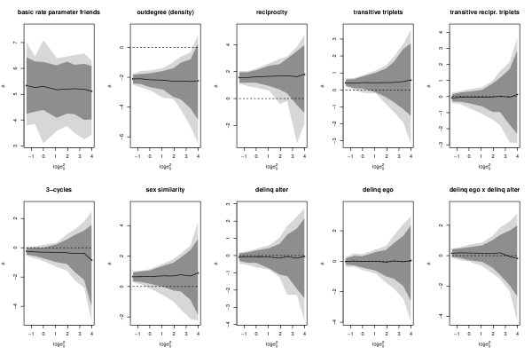
Figure 2: Credibility intervals (95%, dark; 99% light) for $\mu$ with default prior and $\mathbf{\Lambda}_{0}=\sigma^{2}_{0}I$ for different values of $\log(\sigma^{2}_{0})$

The influence on the group parameters $\gamma^{[g]}_{k}$ of the same set of priors is illustrated in Figure 3. Note the difference in vertical scale. The inference on these parameters is remarkably robust to the prior variance. Only for extreme values of $\sigma^{2}_{0}$ and for a few classrooms do we see a big change in group-level parameters. The very wide intervals are due to two specific classrooms. More specifically, in one classroom (number 20) ‘transitive reciprocated triples’ and ‘3-cycles’ were collinear, which manifests itself in extremely large intervals for these parameters when large $\sigma^{2}_{0}$ prevents this classroom from borrowing information from the other classrooms. Another classroom (number 11) had a similar issue with structural parameters and in addition a ‘sex similarity’ effect that is difficult to estimate because of the very skewed sex distribution in this classroom. The issues with these two classrooms also manifests themselves in increasingly poor mixing for $\gamma^{[g]}$ for large values of $\sigma^{2}_{0}$ (results available upon request from the authors).

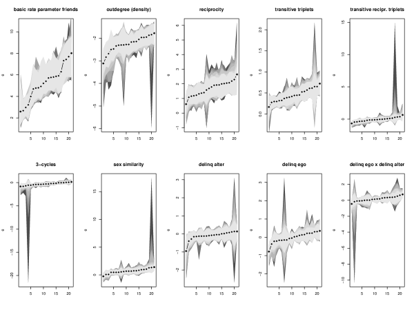
Figure 3: Equal 95% tail prediction intervals for $\gamma^{[g]}$ for different values of $\sigma^{2}_{0}$, from $\sigma^{2}_{0}=0.25$ (light grey) to $\sigma^{2}_{0}=113$ (dark grey). Groups ordered according to posterior predictive mean

B.2 Reference prior

We may consider the influence of the prior for $\mu$ and $\Sigma$ on the predictive distributions for $\gamma^{[g]}$ by comparing these to posteriors from group-level parameters estimated independently. The a priori dependence of $\mu$ on $\Sigma$ can be decoupled by setting $\pi(\mu,\Sigma)=\pi(\mu)\pi(\Sigma)$. When $G>p_{1}+1$, we may chose an improper prior for $(\mu,\Sigma)$ for reference.

Jeffreys rule (Jeffreys, 1998) is a principled choice for a reference prior. For the multivariate normal distribution, it is given by

$$p(\mu,\Sigma)\propto|\Sigma|^{-(p_{1}+2)/2}{\text{ ,}}$$

or (for the independence-Jeffreys prior)

$$p(\mu,\Sigma)\propto|\Sigma|^{-(p_{1}+1)/2}{\text{ .}}$$

For the conjugate model this corresponds to $\kappa_{0}\rightarrow 0$, $\nu_{0}\rightarrow 0$, and letting the determinant of $\Lambda_{0}$ tend to $0$. Jeffreys prior is still conjugate for $\mu$ and $\Sigma$, and as such does not alter the updating scheme outlined in Section 6.

Figure 4 illustrates the inference obtained from (horizontal) fitting the model separately to each classroom, assuming a constant prior, and (vertical) the predictive distributions obtained from the hierarchical SAOM with Jeffreys prior. The two previously mentioned classrooms 11 and 20 are omitted for reasons mentioned above. Both analyses are based on the other 19 classrooms.

Figure 4 demonstrates a negligible influence of the prior on the distributions for $\gamma^{[g]}$. Figure 5 presents the posterior densities for $\mu_{k}$ and shows that these are also centered on the raw, un-weighted means $\bar{\gamma}_{k}$ of $\gamma^{[g]}_{k}$ from the separate estimations. This shows that imposing the multivariate normal model for the group-level parameters does not yield results that differ strongly from the individual group-level inference. In order to make use of all classrooms we would however require more additional classrooms to borrow strength across groups, and impose a more informative prior for $\mu$ and $\Sigma$.

Figure 4: Prediction-intervals for $\gamma^{[g]}$ fitted independently (horizontal axis) against predictions from Hierarchical SAOM using Jeffreys prior (vertical) (excluding classrooms $g=11,20$)

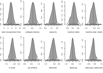
Figure 5: Posteriors for $\mu$ fitted using Jeffreys prior with vertical line representing $\bar{\gamma}_{k}$ and the horizontal bar $\bar{\gamma}_{k}\pm 2sd(\gamma^{[g]}_{k})$ from independently fitting each group (excluding rogue $g=11,20$)

Appendix C Posteriors

For the estimated model of Table 5, Figure 6 presents the posterior distributions of the population mean $\mu_{k}$ for the delinquency outdegree - activity effect and of the constant parameter $\eta_{k}$ for the effect (‘odd’) of same delinquency acts as friends. For both parameters it is evident that they are positive with a high posterior probability. There is less posterior uncertainty about $\mu_{k}$ than $\eta_{k}$ but the former is a population mean of varying group-wise parameters $\gamma_{k}^{[g]}$ whereas the latter is a constant parameter. This variability across groups is illustrated in Figure 7 (right panel), which shows boxplots (without outliers) of the posterior distributions of $\gamma_{k}^{[g]}$ for groups $g$ ordered according to the posterior means, with horizontal credibility bands in grey for $\mu_{k}$. The variability in group-level means is greater than the variability in $\mu_{k}$ but $\gamma^{[g]}$ is clearly positive with high posterior probability for all groups $g$. The length of the 95%CI for delinquency outdegree - activity is $0.072$ and the length of the 95%CI for same language is $0.132$ but both parameters are positive with high posterior probability. There is a greater variation in the group-level parameters for same language, however (Figure 7, left panel), and $\Pr(\gamma^{[g]}>0\mid y)$ ranges from $0.30$ to $1.00$ with a median of $0.88$.

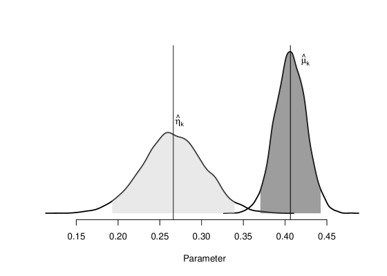
Figure 6: Posterior densities for $\mu_{k}$ for delinquency outdegree - activity and $\eta_{k}$ for same delinquency acts as friends (‘odd’) with 95% credibility intervals in dark and light grey, respectively.

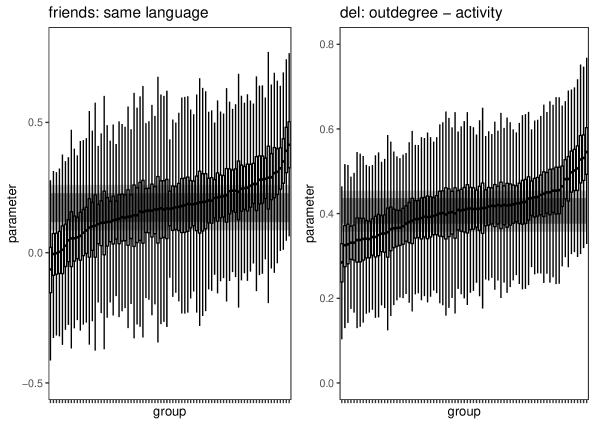
Figure 7: Boxplots (without outliers) for posteriors of $\gamma_{k}^{[g]}$ for same language and delinquency outdegree - activity, ordered by posterior means. The horizontal dark and light grey bands indicate the 90% and 99% credibility intervals for $\mu_{k}$.

References

- Aldous (1983) Aldous, D. (1983) Minimization algorithms and random walk on the d-cube. The Annals of Probability, 11, 403–413.
- Anderson et al. (1999) Anderson, B. S., Butts, C. and Carley, K. (1999) The interaction of size and density with graph-level indices. Social Networks, 21, 239–267.
- Batagelj and Bren (1995) Batagelj, V. and Bren, M. (1995) Comparing resemblance measures. Journal of Classification, 12, 73–90.
- Bergstrom (1988) Bergstrom, A. R. (1988) The history of continuous-time econometric models. Econometric Theory, 4, 365–383.
- Block (2015) Block, P. (2015) Reciprocity, transitivity, and the mysterious three-cycle. Social Networks, 40, 163–173.
- Block et al. (2018) Block, P., Koskinen, J., Hollway, J., Steglich, C. and Stadtfeld, C. (2018) Change we can believe in: comparing longitudinal network models on consistency, interpretability and predictive power. Social Networks, 52, 180–191.
- Boda (2018) Boda, Z. (2018) Social influence on observed race. Sociological Science, 5, 29–57.
- Brandes et al. (2013) Brandes, U., Robins, G., McCranie, A. and Wasserman, S. (2013) What is network science? Network Science, 1, 1–15.
- Dolgova (2019) Dolgova, E. (2019) On Getting Along and Getting Ahead: How Personality Affects Social Network Dynamics. Ph.D. thesis, Erasmus University, Rotterdam. URL: https://repub.eur.nl/pub/119150/Dissertation_Dolgova_final_printer2.pdf.
- Eager and Roy (2017) Eager, C. and Roy, J. (2017) Mixed effects models are sometimes terrible.
- Elmer et al. (2017) Elmer, T., Boda, Z. and Stadtfeld, C. (2017) The co-evolution of emotional well-being with weak and strong friendship ties. Network Science, 5, 278–307.
- Entwisle et al. (2007) Entwisle, B., Faust, K., Rindfuss, R. R. and Kaneda, T. (2007) Networks and contexts: Variation in the structure of social ties. American Journal of Sociology, 112, 1495–1533.
- Erdős and Rényi (1960) Erdős, P. and Rényi, A. (1960) On the evolution of random graphs. A Matematikai Kutató Intézet Kőzleményei, 5, 17–61.
- Faust and Skvoretz (2002) Faust, K. and Skvoretz, J. (2002) Comparing networks across space and time, size and species. Sociological Methodology, 32, 267–299.
- Fujimoto et al. (2018) Fujimoto, K., Snijders, T. and Valente, T. W. (2018) Multivariate dynamics of one-mode and two-mode networks: Explaining similarity in sports participation among friends. Network Science, 6, 370–395.
- Gelman et al. (2014) Gelman, A., Carlin, J. B., Stern, H. S., Dunson, D. B., Vehtari, A. and Rubin, D. B. (2014) Bayesian Data Analysis. Boca Raton, FL: Chapman & Hall / CRC, 3d edn.
- Gelman et al. (1996) Gelman, A., Roberts, G. O. and Gilks, W. R. (1996) Efficient Metropolis jumping rules. In Bayesian Statistics 5 (eds. J. Berardo, J. Berger, A. Dawid and A. Smith), 599–607. Oxford: Clarendon Press.
- Goldstein (2011) Goldstein, H. (2011) Multilevel Statistical Models. London: Edward Arnold, 4th edn.
- Greenan (2015) Greenan, C. C. (2015) Diffusion of innovations in dynamic networks. Journal of the Royal Statistical Society, Series A, 178, 147–166.
- Hamerle et al. (1993) Hamerle, A., Singer, H. and Nagl, W. (1993) Identification and estimation of continuous time dynamic systems with exogenous variables using panel data. Econometric Theory, 9, 283–295.
- Holland and Leinhardt (1977) Holland, P. W. and Leinhardt, S. (1977) A dynamic model for social networks. Journal of Mathematical Sociology, 5, 5–20.
- Huitsing et al. (2014) Huitsing, G., Snijders, T. A., Van Duijn, M. A. and Veenstra, R. (2014) Victims, bullies, and their defenders: A longitudinal study of the coevolution of positive and negative networks. Development and Psychopathology, 26, 645–659.
- Jeffreys (1998) Jeffreys, H. (1998) The theory of probability. OUP Oxford.
- Kalter et al. (2013) Kalter, F., Heath, A. F., Hewstone, M., Jonsson, J. O., Kalmijn, M., Kogan, I. and van Tubergen, F. (2013) Children of immigrants longitudinal survey in four European countries (CILS4EU): Motivation, aims, and design. Tech. rep., GESIS: GESIS Data Archive, Cologne.
- Kivelä et al. (2014) Kivelä, M., Arenas, A., Barthelemy, M., Gleeson, J. P., Moreno, Y. and Porter, M. A. (2014) Multilayer networks. Journal of Complex Networks, 2, 203–271.
- Knecht (2006) Knecht, A. (2006) Networks and actor attributes in early adolescence [2003/04]. Ics-codebook no. 61, The Netherlands Research School ICS, Department of Sociology, University of Utrecht, Utrecht. Persistent data set identifier urn:nbn:nl:ui:13-ehzl-c6.
- Knecht et al. (2010) Knecht, A., Snijders, T. A. B., Baerveldt, C., Steglich, C. and Raub, W. (2010) Friendship and delinquency: Selection and influence processes in early adolescence. Social Development, 19, 494–514.
- Köllisch and Oberwittler (2004) Köllisch, T. and Oberwittler, D. (2004) Wie ehrlich berichten männliche jugendliche über ihr delinquentes verhalten? KZfSS Kölner Zeitschrift für Soziologie und Sozialpsychologie, 56, 708–735.
- Koskinen and Snijders (2007) Koskinen, J. H. and Snijders, T. A. B. (2007) Bayesian inference for dynamic social network data. Journal of Statistical Planning and Inference, 13, 3930–3938.
- Krivitsky et al. (2011) Krivitsky, P. N., Handcock, M. S. and Morris, M. (2011) Adjusting for network size and composition effects in exponential-family random graph models. Statistical Methodology, 8, 319–339.
- Lomi et al. (2011) Lomi, A., Snijders, T. A. B., Steglich, C. and Torlò, V. J. (2011) Why are some more peer than others? Evidence from a longitudinal study of social networks and individual academic performance. Social Science Research, 40, 1506–1520.
- Lomi and Stadtfeld (2014) Lomi, A. and Stadtfeld, C. (2014) Social networks and social settings: Developing a coevolutionary view. KZfSS Kölner Zeitschrift für Soziologie und Sozialpsychologie, 66, 395–415.
- Maddala (1983) Maddala, G. (1983) Limited-dependent and Qualitative Variables in Econometrics. Cambridge: Cambridge University Press, 3rd edn.
- Magnani and Wasserman (2017) Magnani, M. and Wasserman, S. (2017) Introduction to the special issue on multilayer networks. Network Science, 5, 141–143.
- O’Hagan and Forster (2004) O’Hagan, A. and Forster, J. (2004) Bayesian Inference, vol. 2B of Kendall’s Advanced Theory of Statistics. London: Arnold.
- Ripley et al. (2021) Ripley, R. M., Snijders, T. A. B., Bóda, Z., Vörös, A. and Preciado, P. (2021) Manual for Siena version 4.0. Tech. rep., Oxford: University of Oxford, Department of Statistics; Nuffield College. URL: http://www.stats.ox.ac.uk/~snijders/siena/.
- Robins (2015) Robins, G. (2015) Doing social network research: Network-based research design for social scientists. London etc.: Sage.
- Schweinberger (2007) Schweinberger, M. (2007) Statistical Methods for Studying the Evolution of Networks and Behavior. Ph.D. thesis, University of Groningen, Groningen.
- Schweinberger et al. (2020) Schweinberger, M., Krivitsky, P. N., Butts, C. T. and Stewart, J. (2020) Foundations of finite-, super-, and infinite-population random graph inference. Statistical Science, 35, 627–662.
- Shalizi and Rinaldo (2013) Shalizi, C. R. and Rinaldo, A. (2013) Consistency under sampling of exponential random graph models. Annals of Statistics, 41, 508–535.
- Shalizi and Thomas (2011) Shalizi, C. R. and Thomas, A. C. (2011) Homophily and contagion are generically confounded in observational social network studies. Sociological Methods & Research, 40, 211–239.
- Singer (1996) Singer, H. (1996) Continuous-time dynamic models for panel data. In Analysis of Change (eds. U. Engel and J. Reinecke), chap. 6, 113–134. De Gruyter.
- Slaughter and Koehly (2016) Slaughter, A. J. and Koehly, L. M. (2016) Multilevel models for social networks: Hierarchical Bayesian approaches to exponential random graph modeling. Social Networks, 44, 334–345.
- Snijders (2001) Snijders, T. A. B. (2001) The statistical evaluation of social network dynamics. In Sociological Methodology – 2001 (eds. M. E. Sobel and M. P. Becker), vol. 31, 361–395. Boston and London: Basil Blackwell.
- Snijders (2005) — (2005) Models for longitudinal network data. In Models and Methods in Social Network Analysis (eds. P. Carrington, J. Scott and S. Wasserman), chap. 11, 215–247. New York: Cambridge University Press.
- Snijders (2016) — (2016) The multiple flavours of multilevel issues for networks. In Multilevel Network Analysis for the Social Sciences (eds. E. Lazega and T. A. B. Snijders), 15–46. Cham: Springer.
- Snijders (2017) — (2017) Stochastic actor-oriented models for network dynamics. Annual Review of Statistics and Its Application, 4, 343–363.
- Snijders and Baerveldt (2003) Snijders, T. A. B. and Baerveldt, C. (2003) A multilevel network study of the effects of delinquent behavior on friendship evolution. Journal of Mathematical Sociology, 27, 123–151.
- Snijders and Bosker (2012) Snijders, T. A. B. and Bosker, R. J. (2012) Multilevel Analysis: An Introduction to Basic and Advanced Multilevel Modeling. London: Sage, 2nd edn.
- Snijders et al. (2010) Snijders, T. A. B., Koskinen, J. H. and Schweinberger, M. (2010) Maximum likelihood estimation for social network dynamics. Annals of Applied Statistics, 4, 567–588.
- Snijders et al. (2013) Snijders, T. A. B., Lomi, A. and Torlò, V. (2013) A model for the multiplex dynamics of two-mode and one-mode networks, with an application to employment preference, friendship, and advice. Social Networks, 35, 265–276.
- Steglich et al. (2010) Steglich, C. E. G., Snijders, T. A. B. and Pearson, M. A. (2010) Dynamic networks and behavior: Separating selection from influence. Sociological Methodology, 40, 329–393.
- Veenstra et al. (2013) Veenstra, R., Dijkstra, J. K., Steglich, C. and Van Zalk, M. H. (2013) Network–behavior dynamics. Journal of Research on Adolescence, 23, 399–412.
- Wasserman and Faust (1994) Wasserman, S. and Faust, K. (1994) Social Network Analysis: Methods and Applications. New York and Cambridge: Cambridge University Press.